Excel’s IF function is a versatile formula that performs logical tests, returning one value if a condition is true and another if false. With its clear syntax, it’s ideal for checking criteria and can be combined with other functions for complex formulas.
1. Excel IF Statement
The IF function evaluates a logical condition and returns different outputs based on the result,
=IF(condition, value_if_true, value_if_false)
Parameters:
- condition: The logical test (e.g., A1 > 10).
- value_if_true: The output if the condition is true.
- value_if_false: The output if the condition is false.
Supported Operators: <, >, <=, >=, =.
The basic IF formula checks a logical condition and returns one value if the condition is true and another if the condition is false. For example, we can test if a cell's value is greater than a certain number and return custom messages or values based on that condition.
Example Formula:
=IF(A1 > 10, "Greater than 10", "10 or less")
- If A1 contains a value greater than 10, the formula returns "Greater than 10".
- If A1 contains 10 or less, it returns "10 or less".
This basic IF formula helps simplify decision-making in spreadsheets, allowing to categorize or analyze data automatically based on defined conditions.
Note: we have the flexibility to define both the condition and the return values.
3. How to Use IF Function in Excel (With Example)
Suppose we want to determine if all the students in a class PASSED or FAILED their tests based on their scores. Instead of manually checking each student's score, we can define the IF condition for one cell.
Step 1: Enter Data in Spreadsheet
First, open MS Excel and enter the relevant data into our worksheet. For example, the data should include students' names in Column A and their corresponding marks in Column B. We want to check whether each student has passed or failed based on their marks.
 Enter data into the sheet
Now, select the cell where we want to display the pass/fail status. For instance, go to Cell C2 and enter the following formula:
=IF(B2>=35, "Pass", "Fail")
This formula checks if the marks in Cell B2 are greater than or equal to 35. If the condition is true (marks ≥ 35), it will display "Pass" otherwise, it will display "Fail".
.webp) Applying to One Cell
Applying to One CellSelect Cell C2, hover over the bottom-right corner until the cursor changes to a "+" (fill handle), then drag it down to apply the formula to the rest of the column.
.webp) Applying to all the Cells
Applying to all the Cells4. How to Use the IF with AND Function in Excel (With Example)
The IF function with AND in Excel allows we to check multiple conditions at once. It returns a value if all the specified conditions are true and another value if any condition is false.
Syntax:
=IF(AND(condition 1, condition 2), Value if true, Value if false)
For example, =IF(AND(A1>90, B1>90), "A1 Grade", "Fail") will return "A1 Grade" if both A1 and B1 are greater than 90, otherwise, it will return "Fail"..
Step 1: Enter the Data into the Sheet
Start by entering the data into our worksheet. For this example, let's assume Column A contains scores for Subject 1 and Column B contains scores for Subject 2.
 Enter Data into the Sheet
Next, in Cell C2, enter the IF with AND formula to check if both scores are greater than 90.
=IF(AND(A2>90, B2>90), "A1 Grade", "Fail")
This formula checks if both A1 and B1 are greater than 90. If both conditions are true, it will return "A1 Grade"; if either of the conditions is false, it will return "Fail".
 Enter IF with AND Formula
Drag the Formula to apply it to rest of the cells.
 Preview Results
5. How to Use the IF with OR Function in Excel
The IF function with OR in Excel allows we to test multiple conditions and return a result if at least one condition is true. The syntax is:
=IF(OR(condition1, condition2), value_if_true, value_if_false)
For example, if we want to check if a student's score in either Subject 1 or Subject 2 is greater than 90, we can use the OR function. If either condition is true, the formula will return "Pass", otherwise, it will return "Fail".
Step 1: Enter the Data
First, enter the data into our worksheet. For example, let's assume Column A contains the scores for Subject 1 and Column B contains the scores for Subject 2.
 Enter data into the sheet
Now, in Cell C2, enter the IF with OR formula to check if either of the two subject scores is greater than 90:
=IF(OR(A2>90, B2>90), "Pass", "Fail")
This formula will return "Pass" if either A1 or B1 is greater than 90. If neither condition is true, it will return "Fail".
 Enter the IF with OR Formula
Drag down and apply the formula to other rows as well
 Drag down the formula
Note: The IF with OR function in Excel will only evaluate numeric values. If the cell contains text or non-numeric values, it will be considered as TRUE, as Excel treats text as a non-zero value. Ensure that the cells contain only numeric data for accurate evaluations.
6. How to Use the IF with NOT Function in Excel
The IF with NOT function in Excel is used to negate a condition. It returns TRUE if the condition is FALSE and FALSE if the condition is TRUE. Essentially, it reverses the result of the condition being tested. It's syntax is:
=IF(NOT(Condition 1), Value if true, Value if false)
For example, if we want to check whether the color of a ball is not red, the formula would be:
=IF(NOT(A1="Red"), "Selected", "Rejected")
- If A1 is not red, it will return "Selected".
- If A1 is red, it will return "Rejected".
Step 1: Enter Data into the Sheet
First, enter our data. For this example, we'll assume that Column A contains the color of balls.
 Enter data
In Cell B1, enter the IF with NOT formula to check if the ball color is not red. The formula will return "Selected" if the color is not red and "Rejected" if it is red.
=IF(NOT(A1="Red"), "Selected", "Rejected")
This formula checks if the value in A1 is not "Red". If the condition is true (i.e., the ball color is not red), it returns "Selected"; otherwise, it returns "Rejected".
 Use IF with NOT Function
Drag down the formula and Preview Results
 Drag down the Formula and Preview Results
This way, the IF with NOT function allows we to check and reverse the outcome based on a specific condition (in this case, checking if the ball is not red).
7. Nested If Function in Excel with Examples
A Nested IF function in Excel is used when we need to evaluate multiple conditions and return different results based on the conditions. In simple terms, it's a combination of multiple IF functions within one formula to handle more than one condition. The syntax is:
=IF( condition1, Value if true1 ,IF(Condition2, Value if true2, Value if false2)).
Below is an example of the Nested if function.
Step 1: Enter our Data
Let's take a dataset of students with their marks and we have to assign the division based on the marks.
=IF(B2>=60,"1st Division",IF(B2>=30,"2nd Division",IF(B2>=10,"3rd Division","Fail")))
.webp) Enter Formula
Enter FormulaThis formula checks multiple conditions:
- If the marks in B2 are greater than or equal to 60, the formula returns "1st Division".
- If the marks are between 30 and 59 (i.e., B2 >= 30 but less than 60), the formula returns "2nd Division".
- If the marks are between 10 and 29 (i.e., B2 >= 10 but less than 30), the formula returns "3rd Division".
- If the marks are less than 10, the formula returns "Fail".
8. IF Statement to Return Another Cell
In Excel, "return another formula with IF" means using the IF function not just to return static text or numbers but to output the result of another formula. This approach dynamically applies calculations or functions based on specific conditions.
For example:
We want to assign a discount based on the purchase amount in cell B2:
- 20% Discount for purchases of 500 or more.
- 10% Discount for purchases between 200 and 499.
- No Discount for purchases less than 200
Step 1: Open our Spreadsheet and Enter Data
Open Excel with existing data or enter new data and go to the cell where we want the discount to appear (e.g., C2).
 Open Excel and Enter data
Step 2: Start with the First Condition
Type the IF formula:
=IF(B2>=500,"20% Discount"
This checks if the value in B2 is greater than or equal to 500.
If TRUE, it returns "20% Discount".
Step 3: Add the Second Condition
If the first condition is FALSE, add another IF function for the next range using the below formula:
=IF(B2>=500,"20% Discount",IF(B2>=200,"10% Discount"
This checks if the value in B2 is greater than or equal to 200 (but less than 500, since the first condition is FALSE).
If TRUE, it returns "10% Discount".
Step 4: Add the Final Condition
Add a condition for all remaining cases (less than 200), use the below formula:
=IF(B2>=500,"20% Discount",IF(B2>=200,"10% Discount","No Discount"))
If neither of the first two conditions is TRUE, it returns "No Discount".
Step 5: Press Enter
Hit Enter to complete the formula. The formula dynamically calculates the discount based on the value in B2.
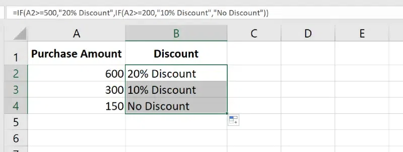 Preview Result
 9. IF Function with Specific Text
When we need to check whether a cell contains specific text, we can use the IF function combined with SEARCH or REGEXMATCH to achieve this. This allows we to perform conditional actions based on whether a given text string exists within another cell.
For example, if we want to check whether a cell contains the word "approved" and return "Yes" if true or "No" if false, we can use:
Step 1: Enter data into the Sheet
Open MS Excel and Enter data into the sheet
 Enter the data
 Select the Cell, where we want to type the Formula and Press Enter
=IF(ISNUMBER(SEARCH("approved",A2)),"Yes","No")
Understand the Components
a) SEARCH("approved", A1):
- Looks for the text "approved" in cell A1.
- If found, it returns the starting position of the text (a number).
- If not found, it returns an error.
b) ISNUMBER(...):
- Checks whether the result of SEARCH is a number (indicating the text was found).
- Returns TRUE if a number exists, otherwise FALSE.
c) IF(ISNUMBER(...),"Yes","No"):
- "Yes" if the text is found.
- "No" if the text is not found.
 Enter the Formula
 Drag down the formula to apply it to other cells as well and preview Results.
 Preview Results
Similar Reads
MS Excel Tutorial - Learn Excel Online Free Excel, one of the powerful spreadsheet programs for managing large datasets, performing calculations, and creating visualizations for data analysis. Developed and introduced by Microsoft in 1985, Excel is mostly used in analysis, data entry, accounting, and many more data-driven tasks.Now, if you ar
11 min read
Excel Fundamental
Introduction to MS ExcelLet’s dive into Microsoft Excel, a versatile spreadsheet tool from the Microsoft Office suite that organizes data into rows and columns. Whether we’re managing budgets, creating charts or analyzing datasets, Excel helps us handle tasks efficiently. For example, we can list project tasks, calculate t
5 min read
Download and Install MS Excel 2024/365 EditionMicrosoft Excel is a tool for data management, reporting, and calculations, widely used by students, professionals, and businesses. The 2024/365 edition offers enhanced features, cloud integration, and improved performance across devices. 1. Downloading Excel 2024/365 on PC or MacExcel is part of Mi
4 min read
Excel SpreadsheetAn Excel spreadsheet, called a workbook, contains one or more worksheets, each a grid of 1,048,576 rows and 16,384 columns for data management. Workbooks organize related data across multiple worksheets in a single file.1. Understanding Excel Workbooks and WorksheetsWorkbook: A single Excel file con
4 min read
Workbooks in Microsoft ExcelA collection of worksheets is referred to as a workbook (spreadsheets). Workbooks are your Excel files. You'll need to create a new workbook every time you start a new project in Excel. There are various ways to begin working with an Excel workbook. You can either start from scratch or use a pre-des
4 min read
Worksheets in ExcelA worksheet is a single spreadsheet in Excel, made up of a grid of rows and columns where data can be entered, calculated, and organized. Each worksheet contains cells where you input text, numbers, or formulas. Worksheets are the main area where work is done in Excel, and multiple worksheets can be
5 min read
Workbooks in Microsoft ExcelA collection of worksheets is referred to as a workbook (spreadsheets). Workbooks are your Excel files. You'll need to create a new workbook every time you start a new project in Excel. There are various ways to begin working with an Excel workbook. You can either start from scratch or use a pre-des
4 min read
Delete All Rows Below Certain Row or Active Cell in ExcelExcel is a tool for storing, analyzing, and creating reports on large datasets. It's widely used by accounting professionals for financial data analysis but is efficient enough for anyone managing large amounts of data. However, dealing with unnecessary rows can clutter our worksheet. Deleting all r
5 min read
How to Remove Hyperlinks in ExcelLooking for the steps to remove unwanted hyperlinks form your Excel worksheet? Then in this short article we are going to discuss 6 different ways to remove hyperlinks in Excel. The steps discussed in this article work in all Excel versions from 2023 to the latest version of Excel.Actually, the HYPE
6 min read
How to Use Fractions in ExcelMicrosoft Excel is a powerful tool for managing numbers, but did you know it can also handle fractions just as smoothly as decimals and whole numbers? If you are a newbie working with data where you need to use fractions, then this guide on how to use fractions will guide you on the practical ways t
6 min read
Excel Formatting
Data Formatting in ExcelData formatting in Excel is the key to transforming raw numbers into clear, professional, and actionable insights. From customizing dates and currencies to applying conditional formatting for quick analysis, mastering these techniques saves time and enhances your spreadsheets’ impact. This guide wil
3 min read
How to Expand Cells to Fit the Text Automatically in ExcelWe all know how useful Excel is to store tabular data. We can do calculations in excel, we can store any information that is in the form of tables, and so on. But there are some common problems that we all face while using Excel. One of the problems that we encounter while entering oversized, overle
3 min read
Excel Date and Time FormatsExcel stores dates as serial numbers and times as fractions of a day, making proper formatting crucial to avoid display errors or calculation issues. This guide explores essential Excel date and time formats, with practical examples like DD/MM/YYYY displays, dynamic timestamps, and formulas for task
4 min read
How to Insert a Picture in a Cell in MS Excel?Every day in business or any other field lots of information are there that are required to store for future use. For anyone, it is very difficult to remember that information for a long time. Earlier data and information are stored in a form of a register, file, or by paperwork but finding it may b
4 min read
How to Unhide and Show Hidden Columns in Excel: Step by Step GuideThere are lots of times when you need to hide certain columns on a temporary basis so you can focus on the specific data. But knowing how to unhide the hidden columns is also important if you want to work on the hidden data again. This complete guide on how to unhide hidden columns in Excel will wal
9 min read
Conditional Formatting in ExcelWe use conditional formatting in Excel to highlight important data based on specific rules. This feature applies colors or styles to cells, helping us spot trends or key values in our spreadsheets effortlessly.We can enhance our data presentation with these practical methods. Let’s explore how to ap
8 min read
Apply Conditional Formatting Based On VLookup in ExcelVLOOKUP is an Excel function to look up data in a table organized vertically. VLOOKUP supports approximate and exact matching and wildcards (* ?) for partial matches.Conditional Formatting Based on VLOOKUP:1. Using the Vlookup formula to compare values in 2 different tables and highlighting those va
3 min read
How to Compare Two Columns and Delete Duplicates in ExcelFacing redundant data in your Excel and don't know how to compare two columns so you can easily de-duplicate Excel? Explore this guide to get the step-by-step instructions to compare two columns and delete duplicate data. Here you will learn multiple ways, like the equal operator, IF() function, and
3 min read
How to Find Duplicate Values in Excel Using VLOOKUPExcel is a great tool for working with data. One of its handy features is the VLOOKUP function, which helps you find matching or duplicate values in your data. In this article, we’ll show you how to use VLOOKUP to spot duplicates in a simple way. You’ll learn how to compare two columns in one sheet,
3 min read
Excel Formula & Function
Basic Excel FormulasWe can make Excel work smarter for us with simple formulas that handle our numbers fast! Whether we’re adding up vegetable costs with =SUM(A1:A5) or finding the average with =AVERAGE(B1:B10), these handy tools help us with budgeting and figuring things out. Let’s get started and learn them together!
3 min read
Use of Concatenate in ExcelThe CONCAT function combines multiple text strings or cell values into one string, supporting dynamic data merging.Syntax:=CONCAT(text1, [text2],)Parameters:text1, text2, ...: The text strings, numbers, or cell references to combine (up to 255 arguments).Note: In older Excel versions, use CONCATENAT
5 min read
Percentage in ExcelExcel’s percentage calculations are vital for data analysis, used by 90% of businesses to track metrics like sales growth or expenses. Calculating percentages is straightforward with formulas like (Part/Whole)*100, such as =A1/B1*100, where A1 is the Part and B1 is the Whole. Excel also offers built
8 min read
Excel LEFT, RIGHT, MID, LEN, and FIND FunctionsLEFT Function in ExcelThe LEFT function returns a given text from the left of our text string based on the number of characters specified.Syntax:LEFT(text, [num_chars])Parameters:Text: The text we want to extract from. Num_chars (Optional): The number of characters we want to extract. Default num_ch
5 min read
Excel IF FunctionExcel’s IF function is a versatile formula that performs logical tests, returning one value if a condition is true and another if false. With its clear syntax, it’s ideal for checking criteria and can be combined with other functions for complex formulas.1. Excel IF Statement The IF function evaluat
10 min read
Excel VLOOKUP FunctionThe term VLOOKUP stands for Vertical Lookup. It is designed to search for a specific value in the first column of a table (lookup column) and retrieve corresponding data from a different column in the same row.Syntax of VLOOKUP Formula:VLOOKUP(lookup_value, table_array, col_index_num, [range_lookup]
12 min read
Dynamic Array Formulas in ExcelDynamic arrays are resizable arrays that calculate automatically and return value into multiple cells based on a formula entered in a single cell. The new array (multiple cells) that we get is known as spilling and the new array has been placed in neighboring cells. It is not necessary to use Ctrl +
2 min read
COUNTIF Function in Excel - Step by Step TutorialExcel’s COUNTIF function is a tool for counting cells that meet specific criteria, streamlining data analysis for tasks like tracking metrics or filtering results. The function, with its simple syntax COUNTIF(range, criteria), counts cells in a specified range based on conditions like text, numbers,
7 min read
How To Use MATCH Function in Excel (With Examples)Finding the right data in large spreadsheets can often feel like searching for a needle in a haystack. This is where the MATCH function in Excel proves invaluable. The MATCH function helps you locate the position of a specific value within a row or column, making it a cornerstone of efficient data m
6 min read
Excel Data Analysis & Visualization
How to Sort by the Last Name in Excel?When you work on excel you'll probably be assigned a task to sort data alphabetically in ascending or descending order and it is quite an easy task to sort data using the first names in either of the order. It is the easiest task to be done in excel. But what if you are given a task to sort a list o
5 min read
How to Sort Data by Color in Excel?Sorting Data By Color allows us to segregate the data cells of a specific color. There can be many ways to sort by color like sorting by Cell color, sorting by Font color, etc. We can also add multiple levels in sorting data by color. Sorting by Color makes analysis very easy and time-saving. Sort b
3 min read
How to Swap Columns in Excel: 3 Methods ExplainedTo Swap Columns in Excel - Quick StepsDrag and Drop: Select a column, drag it to a new position, and release.Cut and Paste: Cut a column (Ctrl + X) for Windows and (Cmd + X) for Mac, then paste it in the new location using Insert Cut Cells.Copy and Paste: Copy a column, then insert the copied cells
8 min read
Sparklines in ExcelSparklines are miniature charts embedded within a single Excel cell. They visually summarize trends, patterns, or data fluctuations, making them ideal for dashboards and compact reports. Unlike traditional charts, sparklines are not separate objects; they exist inside the cell itself, behaving like
8 min read
Pivot Tables in ExcelPivot Tables in Excel are an efficient tool for summarizing, analyzing and organizing large datasets. They enable us to group, filter and perform calculations (e.g., sums, averages) on data using a flexible, drag-and-drop interface, transforming raw data into actionable insights without complex form
3 min read
How to Sort a Pivot Table in Excel : A Complete GuideSorting a Pivot Table in Excel is a powerful way to organize and analyze data effectively. Whether you want to sort alphabetically, numerically, or apply a custom sort in Excel, mastering this feature allows you to extract meaningful insights quickly. This guide walks you through various Pivot Table
7 min read
Pivot Table Slicers in ExcelInserting a Pivot Table Slicer in Excel means adding a visual filter to a Pivot Table, allowing users to quickly and interactively filter data. Slicers use buttons to display specific subsets of data, improving clarity, ease of use, and overall data exploration across one or more Pivot Tables.How to
6 min read
Data Visualizations in Power ViewData visualization is a technique to represent the data or set of information in charts. Excel gives a tool of Power View where we can explore the data interactively and also we can visualize the data such that data can be presented in Tables, Bar charts, Scatter plots, and Pie charts. This tool can
3 min read
Chart Visualizations in Excel Power ViewPower View is an Excel Visualization tool that allows you to build visually appealing graphs and charts, dashboards for management, and reports that can be issued daily, weekly, or monthly. When we think of Microsoft Excel, we think of various tools such as Formulae, which makes an analyst's job sim
8 min read
Table Visualization in Excel Power ViewFor whatever visualization we decide to make with Power View, we start by generating a Table, which is the default, and then quickly convert the Table to other visualizations. The Table is formatted similarly to any other data table, with columns representing fields and rows representing data values
5 min read
Multiple Visualizations in Excel Power ViewPower View allows for interactive data exploration, visualization, and presentation, promoting easy ad hoc reporting. Power View's flexible visuals enable on-the-fly analysis of large data sets. The data visualizations are dynamic, making it easier to show the data with a single Power View report. M
4 min read
How to Create Dynamic Excel Dashboards Using Picklists?Dashboards are a report technique that visually presents critical metrics or a data summary to allow for quick and effective business decisions. Excel is capable of handling complex statistical calculations, many of which are built-in as Functions and can be easily displayed on a dashboard. Excel da
3 min read
Advanced Excel
How to Use Solver in Excel?A solver is a mathematical tool present in MS-Excel that is used to perform calculations by working under some constraints/conditions and then calculates the solution for the problem. It works on the objective cell by changing the variable cells any by using sum constraints. Solver is present in MS-
3 min read
Power Query – Source Reference as File Path in CellPower query helps in doing automation in an efficient manner. It allows users to utilize files stored in specific locations and apply routine transformation steps on those files. It allows users to embed file paths and file sources in an Excel cell. The end user can make use of named ranges and Exce
2 min read
How to Create Relational Tables in Excel?Excel directly doesn't provide us ready to use a database, but we can create one using relationships between various tables. This type of relationship helps us identify the interconnections between the table and helps us whenever a large number of datasets are connected in multiple worksheets. We ca
4 min read
How to Import, Edit, Load and Consolidate Data in Excel Power Query?Power Query is an easy and efficient way of solving simple data tasks. Most of our valuable time is frequently consumed by tedious manual procedures like cut and paste, column merging, and filtering. These operations are greatly simplified with the Power Query tool. A further advantage is that, in c
8 min read
Connecting Excel to SQLiteA tiny, quick, self-contained, highly reliable, fully-featured serverless, zero-configuration, transactional SQL database engine is implemented by SQLite, an in-process C language library. The most popular database engine worldwide is SQLite. The public domain status of SQLite's source code allows f
4 min read
Handling Integers in Advanced ExcelA table can be converted into a chart with the help of a power view where one column of data has to be aggregated. Power View can aggregate both integer and decimal numbers. We can also aggregate the data models by other default behavior. Power View provides Power View Fields where the sigma symbol
2 min read
Power Pivot for ExcelPower Pivot serves as an Excel add-on enabling robust data analysis and the creation of advanced data models. This tool facilitates the integration of extensive data from diverse sources, enabling swift information analysis and seamless sharing of insights. Whether working in Excel or Power Pivot, u
10 min read
Excel Power Pivot - Managing Data ModelPower Pivot is something that helps us in relating between two different data sets which are in two different worksheets. We can manage and relate any type of data using Power Pivot. It is used for data analysis and creates many different data models. we can collect large data from different sheets
6 min read
Table and Chart Combinations in Excel Power PivotFor data exploration, visualization, and reporting, Power Pivot offers a variety of Power PivotTable and Power PivotChart combinations. A Power PivotChart is a PivotChart that was made using the Power Pivot window and is based on the Data Model. Despite sharing certain functionality with Excel Pivot
3 min read
Excel Data Visualization
Advanced Excel - Chart DesignThe charts are the visual representation of data in both rows and columns. They are used to analyze the trends and patterns in the datasets. For example, If we want to analyze the sales of different courses for a specific period of time we can easily do this with the help of charts and get the resul
4 min read
How to Create a Graph in Excel: A Step-by-Step Guide for BeginnersAnyone who wants to quickly make observations and represent them graphically should know how to create graphs with Excel. Whether it is the preparation of business analysis papers, academic research documents or financial reports among other things, learning how to make graphs in Excel can significa
8 min read
Formatting Charts in ExcelOne of the major uses of Excel is to create different types of charts for a given data set. Excel provides us with a lot of modification options to perform on these charts to make them more insightful. In this article, we are going to see the most common "Formatting" performed on charts using a suit
3 min read
How to Create a Waterfall Chart in Excel Waterfall charts are a powerful visualization tool used to illustrate the cumulative effect of sequential data points, such as profits, losses, or changes over time. Widely used in financial and performance analysis, these charts provide clear insights into the contributions of individual components
6 min read
Scatter and Bubble Chart Visualization in ExcelScatter Charts and Bubble Charts display many related data in one Chart. In both of these charts, the X - axis displays one numeric field and the Y-axis displays another. It helps to specify the relationship between two values for all the items in the chart easily. In Bubble charts, a third numeric
5 min read
How to Create a Pie Chart in Excel - Step by Step Guide Pie charts are an excellent way to visualize proportions and illustrate how different components contribute to a whole. Whether you're analyzing market share, budget allocation, or survey results, pie charts make complex data easily understandable at a glance. This guide will walk you through how to
6 min read
How To Create A Pictograph In Excel?The Pictograph is the record consisting of pictorial symbols. Generally, in mathematics, it is represented by the help of graphs with pictures or icons representing certain quantities or numbers of people, books, etc. It is also known as pictogram, pictogramme, pictorial chart, picture graph, or sim
3 min read
How to make a 3 Axis Graph using Excel?3 Axis Graphs in Excel are the graphs that have three axis. The need for a three-axis arises when the scale of the values is very different. For example, you are given an atom and you want to make a graph between its diameter, melting point, and colloidal nature. If they are plotted on the same scal
7 min read
How To Create a Tornado Chart In Excel?Tornado charts are a special type of Bar Charts. They are used for comparing different types of data using horizontal side-by-side bar graphs. They are arranged in decreasing order with the longest graph placed on top. This makes it look like a 2-D tornado and hence the name. Creating a Tornado Char
2 min read
How to Create Flowchart in Excel: Step-by-Step GuideA Flowchart is a valuable tool for visualizing processes, workflows, or decision-making paths, making it easier to communicate ideas and identify improvements. This article provides a clear, step-by-step guide on how to create a Flowchart in Excel, using its shapes and formatting tools to design cus
6 min read
Excel VBA & Macros
How to Insert and Run VBA Code in Excel?In Excel VBA stands for (Visual Basic for Application Code) where we can automate our task with help of codes and codes that will manipulate(like inserting, creating, or deleting a row, column, or graph) the data in a worksheet or workbook. With the help of VBA, we can also automate the task in exce
2 min read
Variables and Data Types in VBA ExcelIn a computer system, variables and data types are almost used in every program to store and represent data. Similarly, Excel VBA also has variables and data types to store and represent data and its type. In this article, we will learn about VBA variables, their scope, data types, and much more. VB
9 min read
How to Use the VBA Editor in Excel: Quick Guide 2024Unlock the full potential of Microsoft Excel by diving into the world of Visual Basic for Applications (VBA). The VBA Editor in Excel is a powerful tool that allows you to automate tasks, create custom functions, and streamline your workflow like never before. Whether you're looking to boost product
7 min read
VBA Strings in ExcelIn Excel's Visual Basic for Applications(VBA), strings are pivotal in handling and manipulating text-based data. Strings serve as a fundamental data type used to store a sequence of characters, enabling the representation of textual information, numbers, symbols, and more. Understanding how VBA hand
8 min read
VBA Find Function in ExcelIn an Excel sheet subset of cells represents the VBA Range which can be single cells or multiple cells. The find function will help to modify our search within its Range object. A specific value in the given range of cells is to search with the help of the Find function. Excel VBA provides different
5 min read
ActiveX Control in Excel VBAWhen we are automating an excel sheet with VBA at that time when the user has a requirement for a more flexible design then it's better to use ActiveX Controller. In Excel user has to add the ActiveX Controller manually and ActiveX Controls are used as objects in codes. There are the following types
3 min read
Multidimensional Arrays in Excel VBAMultidimensional Arrays are used to store data of similar data types of more than one dimension. A multidimensional array has a dimension up to 60 but usually, we don't use arrays of dimensions more than 3 or 4. Here, we will see how to declare a multidimensional array in many ways and also how to c
2 min read
VBA Error HandlingIn a VBA code, there may be some errors like syntax errors, compilation errors, or runtime errors so we need to handle these errors. Suppose there is a code of 200 lines and the code has an error it's very difficult to find an error in the code of 200 lines so it's better to handle the error where w
10 min read
How to Remove Duplicates From Array Using VBA in Excel?Excel VBA code to remove duplicates from a given range of cells. In the below data set we have given a list of 15 numbers in “Column A†range A1:A15. Need to remove duplicates and place unique numbers in column B. Sample Data: Cells A1:A15 Sample Data Final Output: VBA Code to remove duplicates and
2 min read
Macros In Excel With Examples: Step-by-Step TutorialExcel macros are a powerful tool that can automate repetitive tasks, saving you time and increasing productivity. Whether you're trying to enable Excel macros, record a macro in Excel, or automate specific actions within your spreadsheet, macros are an invaluable feature. In this guide, we will walk
11 min read
Assigning Excel Macro to ObjectsIn Excel, a recorded macro can be assigned to different objects like a shape, graphic, or control note. Instead of running the macro from the required tool in ribbon, we can create these objects to run them easily. They get very handy when multiple macros are there. Individual objects can be created
3 min read
How to Enable Macros in Excel (2025): Step-by-Step GuideHow to Activate Macros in Excel - Quick StepsOpen the Excel workbook.Click Enable Content in the yellow security warning bar.Go to File > Options > Trust Center > Trust Center Settings > Macro Settings.Choose the desired macro setting (e.g., Enable All Macros for trusted files).Save the
9 min read
Power BI & Advance Features in Excel