Reduce Data Dimensionality using PCA - Python
Last Updated :
23 Jul, 2025
Introduction
The advancements in Data Science and Machine Learning have made it possible for us to solve several complex regression and classification problems. However, the performance of all these ML models depends on the data fed to them. Thus, it is imperative that we provide our ML models with an optimal dataset. Now, one might think that the more data we provide to our model, the better it becomes - however, it is not the case. If we feed our model with an excessively large dataset (with a large no. of features/columns), it gives rise to the problem of overfitting, wherein the model starts getting influenced by outlier values and noise. This is called the Curse of Dimensionality.
The following graph represents the change in model performance with the increase in the number of dimensions of the dataset. It can be observed that the model performance is best only at an option dimension, beyond which it starts decreasing.
 Model Performance Vs No. of Dimensions (Features) - Curse of Dimensionality
Dimensionality Reduction is a statistical/ML-based technique wherein we try to reduce the number of features in our dataset and obtain a dataset with an optimal number of dimensions.
One of the most common ways to accomplish Dimensionality Reduction is Feature Extraction, wherein we reduce the number of dimensions by mapping a higher dimensional feature space to a lower-dimensional feature space. The most popular technique of Feature Extraction is Principal Component Analysis (PCA)
Principal Component Analysis (PCA)
As stated earlier, Principal Component Analysis is a technique of feature extraction that maps a higher dimensional feature space to a lower-dimensional feature space. While reducing the number of dimensions, PCA ensures that maximum information of the original dataset is retained in the dataset with the reduced no. of dimensions and the co-relation between the newly obtained Principal Components is minimum. The new features obtained after applying PCA are called Principal Components and are denoted as PCi (i=1,2,3...n). Here, (Principal Component-1) PC1 captures the maximum information of the original dataset, followed by PC2, then PC3 and so on.
The following bar graph depicts the amount of Explained Variance captured by various Principal Components. (The Explained Variance defines the amount of information captured by the Principal Components).
 Explained Variance Vs Principal Components
In order to understand the mathematical aspects involved in Principal Component Analysis do check out Mathematical Approach to PCA. In this article, we will focus on how to use PCA in Python for Dimensionality Reduction.
Steps to Apply PCA in Python for Dimensionality Reduction
We will understand the step by step approach of applying Principal Component Analysis in Python with an example. In this example, we will use the iris dataset, which is already present in the sklearn library of Python.
Step-1: Import necessary libraries
All the necessary libraries required to load the dataset, pre-process it and then apply PCA on it are mentioned below:
Python3
# Import necessary libraries
from sklearn import datasets  # to retrieve the iris Dataset
import pandas as pd  # to load the dataframe
from sklearn.preprocessing import StandardScaler  # to standardize the features
from sklearn.decomposition import PCA  # to apply PCA
import seaborn as sns  # to plot the heat maps
Step-2: Load the dataset
After importing all the necessary libraries, we need to load the dataset. Now, the iris dataset is already present in sklearn. First, we will load it and then convert it into a pandas data frame for ease of use.
Python3
#Load the Dataset
iris = datasets.load_iris()
#convert the dataset into a pandas data frame
df = pd.DataFrame(iris['data'], columns = iris['feature_names'])
#display the head (first 5 rows) of the dataset
df.head()
Output:
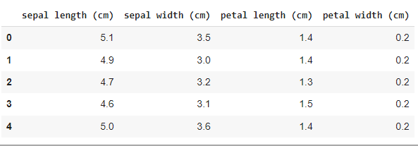 iris dataset
Step-3: Standardize the features
Before applying PCA or any other Machine Learning technique it is always considered good practice to standardize the data. For this, Standard Scalar is the most commonly used scalar. Standard Scalar is already present in sklearn. So, now we will standardize the feature set using Standard Scalar and store the scaled feature set as a pandas data frame.
Python3
#Standardize the features
#Create an object of StandardScaler which is present in sklearn.preprocessing
scalar = StandardScaler()
scaled_data = pd.DataFrame(scalar.fit_transform(df)) #scaling the data
scaled_data
Output:
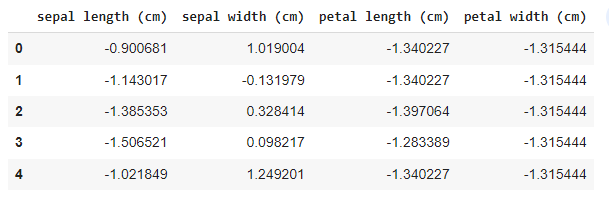 Scaled iris dataset
Step-3: Check the Co-relation between features without PCA (Optional)
Now, we will check the co-relation between our scaled dataset using a heat map. For this, we have already imported the seaborn library in Step-1. The correlation between various features is given by the corr() function and then the heat map is plotted by the heatmap() function. The colour scale on the side of the heatmap helps determine the magnitude of the co-relation. In our example, we can clearly see that a darker shade represents less co-relation while a lighter shade represents more co-relation. The diagonal of the heatmap represents the co-relation of a feature with itself - which is always 1.0, thus, the diagonal of the heatmap is of the highest shade.
Python3
#Check the Co-relation between features without PCA
sns.heatmap(scaled_data.corr())
Output:
 Co-relation Heatmap of Iris dataset without PCA
 We can observe from the above heatmap that sepal length & petal length and petal length & petal width have high co-relation. Thus, we evidently need to apply dimensionality reduction. If you are already aware that your dataset needs dimensionality reduction - you can skip this step.
Step-4: Applying Principal Component Analysis
We will apply PCA on the scaled dataset. For this Python offers yet another in-built class called PCA which is present in sklearn.decomposition, which we have already imported in step-1. We need to create an object of PCA and while doing so we also need to initialize n_components - which is the number of principal components we want in our final dataset. Here, we have taken n_components = 3, which means our final feature set will have 3 columns. We fit our scaled data to the PCA object which gives us our reduced dataset.
Python
#Applying PCA
#Taking no. of Principal Components as 3
pca = PCA(n_components = 3)
pca.fit(scaled_data)
data_pca = pca.transform(scaled_data)
data_pca = pd.DataFrame(data_pca,columns=['PC1','PC2','PC3'])
data_pca.head()
Output:
 PCA Dataset
Step-5: Checking Co-relation between features after PCA
Now that we have applied PCA and obtained the reduced feature set, we will check the co-relation between various Principal Components, again by using a heatmap.
Python3
#Checking Co-relation between features after PCA
sns.heatmap(data_pca.corr())
Output:
 Heatmap after PCA
The above heatmap clearly depicts that there is no correlation between various obtained principal components (PC1, PC2, and PC3). Thus, we have moved from higher dimensional feature space to a lower-dimensional feature space while ensuring that there is no correlation between the so obtained PCs is minimum. Hence, we have accomplished the objectives of PCA.
Advantages of Principal Component Analysis (PCA):
- For efficient working of ML models, our feature set needs to have features with no co-relation. After implementing the PCA on our dataset, all the Principal Components are independent - there is no correlation among them.
- A Large number of feature sets lead to the issue of overfitting in models. PCA reduces the dimensions of the feature set - thereby reducing the chances of overfitting.
- PCA helps us reduce the dimensions of our feature set; thus, the newly formed dataset comprising Principal Components need less disk/cloud space for storage while retaining maximum information.
Similar Reads
Machine Learning Tutorial Machine learning is a branch of Artificial Intelligence that focuses on developing models and algorithms that let computers learn from data without being explicitly programmed for every task. In simple words, ML teaches the systems to think and understand like humans by learning from the data.Do you
5 min read
Introduction to Machine Learning
Python for Machine Learning
Machine Learning with Python TutorialPython language is widely used in Machine Learning because it provides libraries like NumPy, Pandas, Scikit-learn, TensorFlow, and Keras. These libraries offer tools and functions essential for data manipulation, analysis, and building machine learning models. It is well-known for its readability an
5 min read
Pandas TutorialPandas (stands for Python Data Analysis) is an open-source software library designed for data manipulation and analysis. Revolves around two primary Data structures: Series (1D) and DataFrame (2D)Built on top of NumPy, efficiently manages large datasets, offering tools for data cleaning, transformat
6 min read
NumPy Tutorial - Python LibraryNumPy is a core Python library for numerical computing, built for handling large arrays and matrices efficiently.ndarray object – Stores homogeneous data in n-dimensional arrays for fast processing.Vectorized operations – Perform element-wise calculations without explicit loops.Broadcasting – Apply
3 min read
Scikit Learn TutorialScikit-learn (also known as sklearn) is a widely-used open-source Python library for machine learning. It builds on other scientific libraries like NumPy, SciPy and Matplotlib to provide efficient tools for predictive data analysis and data mining.It offers a consistent and simple interface for a ra
3 min read
ML | Data Preprocessing in PythonData preprocessing is a important step in the data science transforming raw data into a clean structured format for analysis. It involves tasks like handling missing values, normalizing data and encoding variables. Mastering preprocessing in Python ensures reliable insights for accurate predictions
6 min read
EDA - Exploratory Data Analysis in PythonExploratory Data Analysis (EDA) is a important step in data analysis which focuses on understanding patterns, trends and relationships through statistical tools and visualizations. Python offers various libraries like pandas, numPy, matplotlib, seaborn and plotly which enables effective exploration
6 min read
Feature Engineering
Supervised Learning
Unsupervised Learning
Model Evaluation and Tuning
Advance Machine Learning Technique
Machine Learning Practice