Generative Modeling in TensorFlow

Generative modeling is the process of learning the underlying structure of a dataset to generate new samples that mimic the distribution of the original data. The article aims to provide a comprehensive overview of generative modelling along with the implementation leveraging the TensorFlow framework.

What are generative models and how do they work?

Generative models aim to learn the probability distribution of data, creating new samples that capture its essence. There are two main ways to define generative models:

Explicit density models

These models explicitly define a probability function for each data point. A Gaussian mixture model, for instance, is an explicit density model that learns the parameters of each Gaussian component and assumes the data is produced by a mixture of Gaussian-distributions. For high-dimensional or you can say complicated data, explicit density models may be computationally expensive or unmanageable, but they may be used to determine the likelihood of every data point.

Implicit density models

These models avoid a defined probability function and instead learn a mapping from a simple latent space to the data space. Generative-Adversarial-Networks (GANs) exemplify this approach, utilizing two networks – a generator and a discriminator – to produce realistic data. Although they create diverse samples calculating the probability of any data point is challenging.

What are the main types of generative models and how are they different?

Generative models are a class of machine learning models that can create new data based on existing data. Different types of generative models have different strengths and weaknesses. Some of the most popular ones are:

Variational Autoencoders (VAEs)

These models compress and decompress data using two neural networks. Additionally, they impose the latent space a straightforward distribution, on the compressed data. In order to get the latent space as near to the simple distribution as feasible and the de-compressed data as similar to the original data as possible, they optimize the model. VAEs may alter and interpolate the latent space in addition to producing smooth and diverse output. However, they may provide distorted/unrealistic data as well as overlook some elements of data distribution.

Generative adversarial networks (GANs)

GANs and other implicit density models (IDMs) employ a game-theoretic approach involving two rival neural networks: a generator that fabricates data in order to deceive a discriminator into believing it to be real. Accurately distinguishing between generated and real data is the discriminator's aim. In order to find a Nash equilibrium, the generator must provide data that the discriminator is unable to distinguish from real data. GANs may learn from incomplete or unlabeled data in addition to being adept at generating accurate and realistic data. They do, however, suffer from mode collapse, where the generator gets stuck producing just a narrow range of data changes, and training instability, where the generator and discriminator's performance fluctuates or diverges.

Autoregressive models (ARMs)

ARMs fall under the category of explicit density models and use a neural network to simulate the conditional probability of each data point while taking the data points that came before it into account. An example of an ARM is a Pixel Recurrent Neural Network (PixelRNN) which creates pictures pixel by pixel by successively anticipating each pixel value based on the ones that came before it. Long-range relationships and complex structures can be captured in the high-quality, diversified data that ARMs can provide. But they might also produce data slowly and in a sequential manner, which could mean they need a lot of computer power and training data.

How to use TensorFlow to build and train generative models?

What if software could create entirely original writings, songs or paintings? Thanks to the field of machine learning called generative modeling this future idea is starting to come true. TensorFlow is an extremely powerful toolkit that you may use to build and train these models on your own ! Use the following essential libraries with TensorFlow to create generative models :

Implementation Steps

1. Model Definition: Specify neural network structure and parameters using TensorFlow's built-in or custom layers. TFP and TFG assist in probabilistic or pre-defined models.
2. Data Preparation: Load and preprocess data using TensorFlow's data API for tasks like batching and transformations. TFH aids with pre-trained models for data processing.
3. Loss and Optimization: Define the loss function and optimizer. TensorFlow provides built-in options, and TFP/TFG support probabilistic alternatives.
4. Training and Evaluation: Train using TensorFlow's loops or custom methods. Evaluate using built-in metrics or custom ones. TFP/TFG assist in training probabilistic models or comparing generative models.

How to evaluate and compare generative models?

Evaluating and comparing generative models can be tricky like judging an art competition with no single " best " answer. While there is no perfect way to measure their creations, these methods can help us understand their strengths and weaknesses:

1. The eye test (Qualitative Evaluation): Visually examining the generated data is required for this, such as contrasting the model paintings with actual ones. With the use of TensorFlow capabilities we can evaluate aspects like variety , sharpness and realism while displaying and saving these pictures. But this is arbitrary and may over-look some subtleties.
2. The numbers game (Quantitative Evaluation): Use the numerical metrics available on tf.keras.metrics and elsewhere. Optionally, use MeanSquaredError() or tf.keras.metrics. Calculate errors and accuracy using the TensorFlow Accuracy() function. using metrics such as Fréchet inception distance, inception score and likelihood. Efficiency and performance are compared using this method. Measures may not adequately capture the true diversity and caliber of generative models if they are selected and applied improperly.

The assessment of generative models ultimately necessitates a harmonious integration of qualitative and quantitative methodologies. We may have a more thorough grasp of these intriguing models and their creative potential by fusing the insights from what the data and our eyes observe.

What are some examples and challenges of generative modeling?

However, generative modeling also faces many challenges and limitations, such as:

Building Basic Autoencoder for Generative Modeling

A generative model that learns to replicate its input into its output is called an autoencoder. It is made up of two components: a decoder that reconstructs the input from the latent representation and an encoder that compresses the input into a latent representation. One may utilize an autoencoder for feature extraction, data compression and dimensionality reduction.

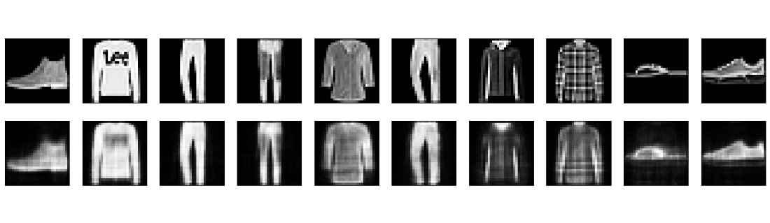
In below example, we'll use a basic autoencoder to compress and decompress the Fashion MNIST dataset which comprises 28x28 grayscale photos of clothes.

Step 1: Add libraries such as TensorFlow.

TensorFlow will be our main framework for developing and optimizing the autoencoder. Among the other tools we'll be utilizing for data processing and visualization are pandas, matplotlib, and numpy.

import tensorflow as tf
import numpy as np
import matplotlib.pyplot as plt
import pandas as pd

Step 2: Load and prepare the dataset

TensorFlow provides the Fashion MNIST dataset, which we will utilize. The training and testing sets will be loaded and the pixel values will be normalized to the interval [-1, 1]. Since our autoencoder uses a single neuron for the output layer. We will also restructure the pictures to have a single channel.

# Load the dataset
(x_train, _), (x_test, _) = tf.keras.datasets.fashion_mnist.load_data()

# Normalize the pixel values
x_train = x_train.astype('float32') / 255.0 * 2 - 1
x_test = x_test.astype('float32') / 255.0 * 2 - 1

# Reshape the images to have a single channel
x_train = x_train.reshape(x_train.shape[0], 28, 28, 1)
x_test = x_test.reshape(x_test.shape[0], 28, 28, 1)

Step 3: Define the model architecture and parameters

Two thick layers—one for the encoder and one for the decoder—will be used in our straightforward autoencoder. 64 neurons make up the encoder, which maps the input to a 64-dimensional latent space using a sigmoid activation function. In order to map the latent space back to the original picture space of 784 dimensions (28x28 pixels). The decoder will employ a tan h activation function with 784 neurons.

Model definition will be done via the Keras Sequential API and model compilation will be done using an Adam optimizer and a mean squared error loss function.

# Define the model architecture
model = tf.keras.Sequential([
  # Encoder layer
  tf.keras.layers.Flatten(input_shape=(28, 28, 1)),
  tf.keras.layers.Dense(64, activation='sigmoid'),
  # Decoder layer
  tf.keras.layers.Dense(784, activation='tanh'),
  tf.keras.layers.Reshape((28, 28, 1))
])

# Compile the model
model.compile(loss='mse', optimizer='adam')

Step 4: Train and evaluate the model

Using a batch size of 256 and a validation split of 0.2. We will train the model across ten epochs. After every epoch, the model weights will be saved using a callback method. In order to assess the model we will compute the reconstruction error on the test set and display a few of the original and rebuilt photos.

# Define a callback function to save the model weights
class SaveModel(tf.keras.callbacks.Callback):
  def on_epoch_end(self, epoch, logs=None):
    model.save_weights(f'autoencoder_{epoch+1}.h5')
    print(f'Saved model weights for epoch {epoch+1}')

# Train the model
model.fit(x_train, x_train, epochs=10, batch_size=256, validation_split=0.2, callbacks=[SaveModel()])

# Evaluate the model
test_loss = model.evaluate(x_test, x_test)
print(f'Test loss: {test_loss}')

# Visualize some of the original and reconstructed images
n = 10 # Number of images to display
plt.figure(figsize=(20, 4))
for i in range(n):
  # Display original image
  ax = plt.subplot(2, n, i + 1)
  plt.imshow(x_test[i].reshape(28, 28), cmap='gray')
  ax.get_xaxis().set_visible(False)
  ax.get_yaxis().set_visible(False)

  # Display reconstructed image
  ax = plt.subplot(2, n, i + 1 + n)
  reconstructed = model.predict(x_test[i].reshape(1, 28, 28, 1))
  plt.imshow(reconstructed.reshape(28, 28), cmap='gray')
  ax.get_xaxis().set_visible(False)
  ax.get_yaxis().set_visible(False)
plt.show()

Output:

Epoch 1/10
188/188 [==============================] - ETA: 0s - loss: 0.2156Saved model weights for epoch 1
188/188 [==============================] - 4s 16ms/step - loss: 0.2156 - val_loss: 0.1324
Epoch 2/10
186/188 [============================>.] - ETA: 0s - loss: 0.1129Saved model weights for epoch 2
188/188 [==============================] - 3s 18ms/step - loss: 0.1128 - val_loss: 0.0990
Epoch 3/10
185/188 [============================>.] - ETA: 0s - loss: 0.0908Saved model weights for epoch 3
188/188 [==============================] - 3s 15ms/step - loss: 0.0907 - val_loss: 0.0839
.
.
.
Epoch 8/10
185/188 [============================>.] - ETA: 0s - loss: 0.0556Saved model weights for epoch 8
188/188 [==============================] - 2s 13ms/step - loss: 0.0556 - val_loss: 0.0546
Epoch 9/10
185/188 [============================>.] - ETA: 0s - loss: 0.0529Saved model weights for epoch 9
188/188 [==============================] - 3s 14ms/step - loss: 0.0529 - val_loss: 0.0522
Epoch 10/10
187/188 [============================>.] - ETA: 0s - loss: 0.0506Saved model weights for epoch 10
188/188 [==============================] - 3s 16ms/step - loss: 0.0506 - val_loss: 0.0501
313/313 [==============================] - 1s 2ms/step - loss: 0.0501
Test loss: 0.050077132880687714

Building Image denoising

The process of removing noise from a picture, which might include many kinds of such speckle, salt-and-pepper, and Gaussian noise, is known as image denoising. Image denoising can enhance an image clarity and quality or get it ready for other uses, such segmentation or classification.

We will use a neural autoencoder to denoise the same MNIST dataset in this case. The autoencoder will be taught to separate the clean pictures from the noisy ones once the original photographs are exposed to Gaussian noise.

Step 1: Import TensorFlow and other libraries.

import tensorflow as tf
import numpy as np
import matplotlib.pyplot as plt
import pandas as pd

Step 2: Load and prepare the dataset

# Load the dataset
(x_train, _), (x_test, _) = tf.keras.datasets.fashion_mnist.load_data()

# Normalize the pixel values
x_train = x_train.astype('float32') / 255.0
x_test = x_test.astype('float32') / 255.0

# Reshape the images to have a single channel
x_train = x_train.reshape(x_train.shape[0], 28, 28, 1)
x_test = x_test.reshape(x_test.shape[0], 28, 28, 1)

# Add Gaussian noise to the images
noise_factor = 0.1
x_train_noisy = x_train + noise_factor * np.random.normal(loc=0.0, scale=1.0, size=x_train.shape)
x_test_noisy = x_test + noise_factor * np.random.normal(loc=0.0, scale=1.0, size=x_test.shape)

# Clip the noisy images to the range [0, 1]
x_train_noisy = np.clip(x_train_noisy, 0.0, 1.0)
x_test_noisy = np.clip(x_test_noisy, 0.0, 1.0)

Step 3: Define the model architecture and parameters

Four convolutional layers—two for the encoder and two for the decoder—will be used in our convolutional autoencoder. By using 32 and 16 filters, together with a kernel size of 3 and a stride of 2. The encoder will cut the input's spatial dimensions in half. The input spatial dimensions will be increased by half thanks to the decoder employment of 16 and 1 filters, a kernel size of 3, and a stride of 2. A sigmoid activation function will also be used by the decoder to map the output to the range [0, 1].

# Define the encoder
def encoder(inputs):
  # Convolutional layer with 32 filters, 3x3 kernel, and 2x2 stride
  x = tf.keras.layers.Conv2D(32, 3, 2, padding='same')(inputs)
  # Convolutional layer with 16 filters, 3x3 kernel, and 2x2 stride
  x = tf.keras.layers.Conv2D(16, 3, 2, padding='same')(x)
  return x

# Define the decoder
def decoder(inputs):
  # Convolutional transpose layer with 16 filters, 3x3 kernel, and 2x2 stride
  x = tf.keras.layers.Conv2DTranspose(16, 3, 2, padding='same')(inputs)
  # Convolutional transpose layer with 1 filter, 3x3 kernel, and 2x2 stride
  x = tf.keras.layers.Conv2DTranspose(1, 3, 2, padding='same', activation='sigmoid')(x)
  return x

# Define the input layer
inputs = tf.keras.layers.Input(shape=(28, 28, 1))

# Define the model
model = tf.keras.Model(inputs=inputs, outputs=decoder(encoder(inputs)))

# Compile the model
model.compile(loss='mse', optimizer='adam')

Step 4: Train and evaluate the model

Using a batch size of 128 and a validation split of 0.2. We will train the model for 50 epochs. After every epoch, the model weights will be saved using a callback method. In order to assess the model , we will compute the reconstruction error on the test set and visualize a portion of the noisy, original photos that have been denoised.

# Define a callback function to save the model weights
class SaveModel(tf.keras.callbacks.Callback):
  def on_epoch_end(self, epoch, logs=None):
    model.save_weights(f'denoising_{epoch+1}.h5')
    print(f'Saved model weights for epoch {epoch+1}')

# Train the model
model.fit(x_train_noisy, x_train, epochs=50, batch_size=128, validation_split=0.2, callbacks=[SaveModel()])

# Evaluate the model
test_loss = model.evaluate(x_test_noisy, x_test)
print(f'Test loss: {test_loss}')

# Visualize some of the original, noisy, and denoised images
n = 10 # Number of images to display
plt.figure(figsize=(20, 6))
for i in range(n):
  # Display original image
  ax = plt.subplot(3, n, i + 1)
  plt.imshow(x_test[i].reshape(28, 28), cmap='gray')
  ax.get_xaxis().set_visible(False)
  ax.get_yaxis().set_visible(False)

  # Display noisy image
  ax = plt.subplot(3, n, i + 1 + n)
  plt.imshow(x_test_noisy[i].reshape(28, 28), cmap='gray')
  ax.get_xaxis().set_visible(False)
  ax.get_yaxis().set_visible(False)

  # Display denoised image
  ax = plt.subplot(3, n, i + 1 + 2 * n)
  denoised = model.predict(x_test_noisy[i].reshape(1, 28, 28, 1))
  plt.imshow(denoised.reshape(28, 28), cmap='gray')
  ax.get_xaxis().set_visible(False)
  ax.get_yaxis().set_visible(False)
plt.show()

Output:

Epoch 1/50
375/375 [==============================] - ETA: 0s - loss: 0.0316Saved model weights for epoch 1
375/375 [==============================] - 24s 60ms/step - loss: 0.0316 - val_loss: 0.0102
Epoch 2/50
375/375 [==============================] - ETA: 0s - loss: 0.0082Saved model weights for epoch 2
375/375 [==============================] - 16s 43ms/step - loss: 0.0082 - val_loss: 0.0069
Epoch 3/50
374/375 [============================>.] - ETA: 0s - loss: 0.0063Saved model weights for epoch 3
375/375 [==============================] - 13s 34ms/step - loss: 0.0063 - val_loss: 0.0060
.
.
.
Epoch 48/50
375/375 [==============================] - ETA: 0s - loss: 0.0049Saved model weights for epoch 48
375/375 [==============================] - 13s 36ms/step - loss: 0.0049 - val_loss: 0.0049
Epoch 49/50
375/375 [==============================] - ETA: 0s - loss: 0.0049Saved model weights for epoch 49
375/375 [==============================] - 13s 34ms/step - loss: 0.0049 - val_loss: 0.0049
Epoch 50/50
374/375 [============================>.] - ETA: 0s - loss: 0.0049Saved model weights for epoch 50
375/375 [==============================] - 12s 33ms/step - loss: 0.0049 - val_loss: 0.0049
313/313 [==============================] - 2s 5ms/step - loss: 0.0050
Test loss: 0.004958466626703739

Conclusion

We have learnt how to utilize TensorFlow for generative modeling in this article. We have also seen two example code with step by step implementation using TensorFlow for generative modeling. This is just a glimpse into the exciting world of generative modeling with TensorFlow. With practice and exploration, you can use this powerful tool to bring your creative ideas to life from generating futuristic landscapes to composing new musical styles.