Concurrency and Parallelism, Asynchronous Programming, Network Programming

DEPARTMENT OF COMPUTER SCIENCE AND ENGINEERING
VELAGAPUDI RAMAKRISHNA SIDDHARTHA ENGINEERING COLLEGE
20CSH4801A
ADVANCED PYTHON PROGRAMMING
UNIT 3
Lecture By,
Prabu. U
Assistant Professor,
Department of Computer Science and Engineering.

UNIT 3:
Concurrency and Parallelism: Introduction to Concurrency and
Parallelism, Threading, Multiprocessing, Inter Thread/Process
Synchronisation, Futures, Concurrency with Async-IO.
Asynchronous Programming: Reactive Programming Introduction,
RxPy Observables, Observers and Subjects, RxPy Operators.
Network Programming: Introduction to Sockets, Sockets in Python.
20CSH4801A ₋ ADVANCED PYTHON PROGRAMMING

1. Introduction to Concurrency and Parallelism
2. Threading
3. Multiprocessing
4. Inter Thread/Process Synchronisation
5. Futures
6. Concurrency with AsyncIO
CONCURRENCY AND PARALLELISM

1. Introduction to Concurrency and Parallelism
(i) Introduction
(ii) Concurrency
(iii) Parallelism
(iv) Distribution
(v) Grid Computing
(vi) Concurrency and Synchronisation
(vii)Object Orientation and Concurrency
(viii)Threads versus Processes
(ix) Some Terminology

(i) Introduction
 In this chapter we will introduce the concepts of concurrency and parallelism.
 We will also briefly consider the related topic of distribution.
 After this we will consider process synchronisation, why object-oriented
approaches are well suited to concurrency and parallelism before finishing
with a short discussion of threads versus processes.

(ii) Concurrency
 Concurrency is defined by the dictionary as two or more events or
circumstances happening or existing at the same time.
 In Computer Science concurrency refers to the ability of different parts or
units of a program, algorithm or problem to be executed at the same time,
potentially on multiple processors or multiple cores.
 Here a processor refers to the central processing unit (or CPU) or a computer
while core refers to the idea that a CPU chip can have multiple cores or
processors on it.
 Originally a CPU chip had a single core. That is the CPU chip had a single
processing unit on it.

 However, over time, to increase computer performance, hardware
manufacturers added additional cores or processing units to chips.
 Thus, a dual-core CPU chip has two processing units while a quad-core CPU
chip has four processing units. This means that as far as the operating system of
the computer is concerned, it has multiple CPUs on which it can run programs.
 Running processing at the same time, on multiple CPUs, can substantially
improve the overall performance of an application.
 For example, let us assume that we have a program that will call three
independent functions, these functions are:
 make a backup of the current data held by the program,
 print the data currently held by the program,
 run an animation using the current data.

 Let us assume that these functions run sequentially, with the following timings:
 the backup function takes 13 s,
 the print function takes 15 s,
 the animation function takes 10 s.
 This would result in a total of 38 s to perform all three operations. This is
illustrated graphically below:
 However, the three functions are all completely independent of each other.
 That is, they do not rely on each other for any results or behaviour; they do not
need one of the other functions to complete before they can complete etc. Thus,
we can run each function concurrently.

Concurrency and Parallelism, Asynchronous Programming, Network Programming

 If the underlying operating system and program language being used support
multiple processes, then we can potentially run each function in a separate
process at the same time and obtain a significant speed up in overall execution
time.
 If the application starts all three functions at the same time, then the maximum
time before the main process can continue will be 15s, as that is the time taken
by the longest function to execute.
 However, the main program may be able to continue as soon as all three
functions are started as it also does not depend on the results from any of the
functions; thus, the delay may be negligible (although there will typically be
some small delay as each process is set up). This is shown graphically below:

(iii) Parallelism
 A distinction its often made in Computer Science between concurrency and
parallelism.
 In concurrency, separate independent tasks are performed potentially at the
same time.
 In parallelism, a large complex task is broken down into a set of subtasks. The
subtasks represent part of the overall problem. Each subtask can be executed
at the same time.
 Typically, it is necessary to combine the results of the subtasks together to
generate an overall result.

 These subtasks are also very similar if not functionally exactly the same
(although in general each subtask invocation will have been supplied with
different data).
 Thus, parallelism is when multiple copies of the same functionality are run at
the same time, but on different data.
 Some examples of where parallelism can be applied include:
 A web search engine. Such a system may look at many, many web pages.
Each time it does so it must send a request to the appropriate web site,
receive the result and process the data obtained. These steps are the same
whether it is the BBC web site, Microsoft’s web site or the web site of
Cambridge University. Thus, the requests can be run sequentially or in
parallel.
 Image Processing. A large image may be broken down into slices so that each
slice can be analysed in parallel.

 The following diagram illustrates the basic idea behind parallelism; a main
program fires off three subtasks each of which runs in parallel. The main
program then waits for all the subtasks to complete before combining together
the results from the subtasks before it can continue.

(iv) Distribution
 When implementing a concurrent or parallel solution, where the resulting
processes run is typically an implementation detail.
 Conceptually these processes could run on the same processor, physical
machine or on a remote or distributed machine.
 As such distribution, in which problems are solved or processes executed by
sharing the work across multiple physical machines, is often related to
concurrency and parallelism.
 However, there is no requirement to distribute work across physical machines,
indeed in doing so extra work is usually involved.

 To distribute work to a remote machine, data and in many cases code, must be
transferred and made available to the remote machine.
 This can result in significant delays in running the code remotely and may
offset any potential performance advantages of using a physically separate
computer.
 As a result, many concurrent/ parallel technologies default to executing code in
a separate process on the same machine.

(v) Grid Computing
 Grid Computing is based on the use of a network of loosely coupled
computers, in which each computer can have a job submitted to it, which it
will run to completion before returning a result.
 In many cases the grid is made up of a heterogeneous set of computers (rather
than all computers being the same) and may be geographically dispersed.
These computers may be comprised of both physical computers and virtual
machines.
 A Virtual Machine is a piece of software that emulates a whole computer and
runs on some underlying hardware that is shared with other virtual machines.

 Each Virtual Machine thinks it is the only computer on the hardware; however
the virtual machines all share the resources of the physical computer.
 Multiple virtual machines can thus run simultaneously on the same physical
computer.
 Each virtual machine provides its own virtual hardware, including CPUs,
memory, hard drives, network interfaces and other devices.
 The virtual hardware is then mapped to the real hardware on the physical
machine which saves costs by reducing the need for physical hardware systems
along with the associated maintenance costs, as well as reducing the power and
cooling demands of multiple computers.

 Within a grid, software is used to manage the grid nodes and to submit jobs to
those nodes.
 Such software will receive the jobs to perform (programs to run and
information about the environment such as libraries to use) from clients of the
grid.
 These jobs are typically added to a job queue before a job scheduler submits
them to a node within the grid.
 When any results are generated by the job they are collected from the node and
returned to the client.
 This is illustrated below:

 The use of grids can make distributing concurrent/parallel processes amongst a
set of physical and virtual machines much easier.

(vi) Concurrency and Synchronisation
 Concurrency relates to executing multiple tasks at the same time. In many
cases these tasks are not related to each other such as printing a document and
refreshing the User Interface.
 In these cases, the separate tasks are completely independent and can execute
at the same time without any interaction.
 In other situations, multiple concurrent tasks need to interact; for example,
where one or more tasks produce data, and one or more other tasks consume
that data.
 This is often referred to as a producer-consumer relationship.

 In other situations, all parallel processes must have reached the same point
before some other behaviour is executed.
 Another situation that can occur is where we want to ensure that only one
concurrent task executes a piece of sensitive code at a time; this code must
therefore be protected from concurrent access.
 Concurrent and parallel libraires need to provide facilities that allow for such
synchronisation to occur.

(vii) Object Orientation and Concurrency
 The concepts behind object-oriented programming lend themselves
particularly well to the concepts associated with concurrency.
 For example, a system can be described as a set of discrete objects
communicating with one another when necessary.
 In Python, only one object may execute at any one moment in time within a
single interpreter. However, conceptually at least, there is no reason why this
restriction should be enforced.
 The basic concepts behind object orientation still hold, even if each object
executes within a separate independent process.

 Traditionally a message send is treated like a procedural call, in which the
calling object’s execution is blocked until a response is returned.
 However, we can extend this model quite simply to view each object as a
concurrently executable program, with activity starting when the object is
created and continuing even when a message is sent to another object (unless
the response is required for further processing).
 In this model, there may be very many (concurrent) objects executing at the
same time.
 Of course, this introduces issues associated with resource allocation, etc. but no
more so than in any concurrent system.

 One implication of the concurrent object model is that objects are larger than in
the traditional single execution thread approach, because of the overhead of
having each object as a separate thread of execution.
 Overheads such as the need for a scheduler to handling these execution threads
and resource allocation mechanisms means that it is not feasible to have
integers, characters, etc. as separate processes.

(viii) Threads versus Processes
 A process is an instance of a computer program that is being executed by the
operating system.
 Any process has three key elements; the program being executed, the data
used by that program (such as the variables used by the program) and the
state of the process (also known as the execution context of the program).
 A (Python) Thread is a preemptive lightweight process.
 A Thread is considered to be pre-emptive because every thread has a chance to
run as the main thread at some point.

 When a thread gets to execute then it will execute until
 completion,
 until it is waiting for some form of I/O (Input/Output),
 sleeps for a period of time,
 it has run for 15 ms (the current threshold in Python 3).
 If the thread has not completed when one of the above situations occurs, then it
will give up being the executing thread and another thread will be run instead.
 This means that one thread can be interrupted in the middle of performing a
series of related steps.

 A thread is a considered a lightweight process because it does not possess its
own address space and it is not treated as a separate entity by the host
operating system.
 Instead, it exists within a single machine process using the same address space.
 It is useful to get a clear idea of the difference between a thread (running within
a single machine process) and a multi-process system that uses separate
processes on the underlying hardware.

(ix) Some Terminology
 The world of concurrent programming is full of terminology that you may not
be familiar with. Some of those terms and concepts are outlined below:
Asynchronous versus Synchronous invocations:
 Most of the method, function or procedure invocations you will have seen in
programming represent synchronous invocations.
 A synchronous method or function call is one which blocks the calling code
from executing until it returns. Such calls are typically within a single thread
of execution.
 Asynchronous calls are ones where the flow of control immediately returns to
the callee, and the caller is able to execute in its own thread of execution.
Allowing both the caller and the call to continue processing.

Non-Blocking versus Blocking code:
 Blocking code is a term used to describe the code running in one thread of
execution, waiting for some activity to complete which causes one of more
separate threads of execution to also be delayed.
 For example, if one thread is the producer of some data and other threads are
the consumers of that data, then the consumer threads cannot continue until
the producer generates the data for them to consume.
 In contrast, non-blocking means that no thread is able to indefinitely delay
others.

Concurrent versus Parallel code:
 Concurrent code and parallel code are similar, but different in one significant
aspect. Concurrency indicates that two or more activities are both making
progress even though they might not be executing at the same point in time.
 This is typically achieved by continuously swapping competing processes
between execution and non-execution. This process is repeated until at least one
of the threads of execution (Threads) has completed their task.
 This may occur because two threads are sharing the same physical processor
with each is being given a short time period in which to progress before the
other gets a short time period to progress.
 The two threads are said to be sharing the processing time using a technique
known as time slicing. Parallelism on the other hand implies that there are
multiple processors available allowing each thread to execute on their own
processor simultaneously.

2. Threading
(i) Introduction
(ii) Threads
(iii) Thread States
(iv) Creating a Thread
(v) Instantiating the Thread Class
(vi) The Thread Class
(vii)The Threading Module Functions
(viii)Passing Arguments to a Thread
(ix) Extending the Thread Class

2. Threading
(x) Daemon Threads
(xi) Naming Threads
(xii) Thread Local Data
(xiii) Timers
(xiv) The Global Interpreter Lock

(i) Introduction
 Threading is one of the ways in which Python allows you to write programs
that multitask; that is appearing to do more than one thing at a time.
 This chapter presents the threading module and uses a short example to
illustrate how these features can be used.

(ii) Threads
 In Python the Thread class from the threading module represents an
activity that is run in a separate thread of execution within a single process.
 These threads of execution are lightweight, pre-emptive execution threads.
 A thread is lightweight because it does not possess its own address space and
it is not treated as a separate entity by the host operating system; it is not a
process.
 Instead, it exists within a single machine process using the same address space
as other threads.

(iii) Threads States
 When a thread object is first created it exists, but it is not yet runnable; it must
be started.
 Once it has been started it is then runnable; that is, it is eligible to be
scheduled for execution.
 It may switch back and forth between running and being runnable under the
control of the scheduler.
 The scheduler is responsible for managing multiple threads that all wish to
grab some execution time.

 A thread object remains runnable or running until its run() method terminates;
at which point it has finished its execution and it is now dead.
 All states between un-started and dead are considered to indicate that the
Thread is alive (and therefore may run at some point). This is shown below:

 A Thread may also be in the waiting state; for example, when it is waiting for
another thread to finish its work before continuing (possibly because it needs
the results produced by that thread to continue).
 This can be achieved using the join() method and is also illustrated above. Once
the second thread completes the waiting thread will again become runnable.
 The thread which is currently executing is termed the active thread.
 There are a few points to note about thread states:
 A thread is considered to be alive unless its run() method terminates after
which it can be considered dead.
 A live thread can be running, runnable, waiting, etc.

 The runnable state indicates that the thread can be executed by the processor,
but it is not currently executing. This is because an equal or higher priority
process is already executing, and the thread must wait until the processor
becomes free. Thus, the diagram shows that the scheduler can move a thread
between the running and runnable state. In fact, this could happen many
times as the thread executes for a while, is then removed from the processor
by the scheduler and added to the waiting queue, before being returned to
the processor again at a later date.

(iv) Creating Threads
 There are two ways in which to initiate a new thread of execution:
 Pass a reference to a callable object (such as a function or method) into the
Thread class constructor. This reference acts as the target for the Thread to
execute.
 Create a subclass of the Thread class and redefine the run() method to
perform the set of actions that the thread is intended to do.
 We will look at both approaches.

 As a thread is an object, it can be treated just like any other object: it can be sent
messages, it can have instance variables and it can provide methods.
 Thus, the multi-threaded aspects of Python all conform to the object-oriented
model.
 This greatly simplifies the creation of multi-threaded systems as well as the
maintainability and clarity of the resulting software.
 Once a new instance of a thread is created, it must be started. Before it is
started, it cannot run, although it exists.

(v) Instantiating the Thread Class
 The Thread class can be found in the threading module and therefore must
be imported prior to use. The class Thread defines a single constructor that
takes up to six optional arguments:
class threading.Thread(group=None,
target=None,
name=None,
args=(),
kwargs={},
daemon=None)

 The Thread constructor should always be called using keyword arguments; the
meaning of these arguments is:
 group should be None; reserved for future extension when a ThreadGroup
class is implemented.
 target is the callable object to be invoked by the run() method. Defaults to
None, meaning nothing is called.
 name is the thread name. By default, a unique name is constructed of the
form “Thread-N” where N is an integer.
 args is the argument tuple for the target invocation. Defaults to (). If a single
argument is provided the tuple is not required. If multiple arguments are
provided then each argument is an element within the tuple.
 kwargs is a dictionary of keyword arguments for the target invocation.
Defaults to {}.
 daemon indicates whether this thread runs as a daemon thread or not. If not
None, daemon explicitly sets whether the thread is daemonic. If None (the
default), the daemonic property is inherited from the current thread.

 Once a Thread is created it must be started to become eligible for execution
using the Thread.start() method.
 The following illustrates a very simple program that creates a Thread that will
run the simple_worker() function:
from threading import Thread
def simple_worker():
print('hello')
# Create a new thread and start it
# The thread will run the function simple_worker
t1 = Thread(target=simple_worker)
t1.start()
 Refer SimpleWorkerEx.py

 In this example, the thread t1 will execute the function simple_worker. The
main code will be executed by the main thread that is present when the
program starts; there are thus two threads used in the above program; main
and t1.

(vi) The Thread Class
 The Thread class defines all the facilities required to create an object that can
execute within its own lightweight process. The key methods are:
 start() Start the thread’s activity. It must be called at most once per
thread object. It arranges for the object’s run() method to be invoked in a
separate thread of control. This method will raise a RuntimeError if called
more than once on the same thread object.
 run() Method representing the thread’s activity. You may override this
method in a subclass. The standard run() method invokes the callable
object passed to the object’s constructor as the target argument, if any, with
positional and keyword arguments taken from the args and kwargs
arguments, respectively. You should not call this method directly.

 join(timeout = None)Wait until the thread sent this message
terminates. This blocks the calling thread until the thread whose
join()method is called terminates. When the timeout argument is present
and not None, it should be a floating-point number specifying a timeout for
the operation in seconds (or fractions thereof). A thread can be join()ed
many times.
 name A string used for identification purposes only. It has no semantics.
Multiple threads may be given the same name. The initial name is set by the
constructor. Giving a thread a name can be useful for debugging purposes.
 ident The ‘thread identifier’ of this thread or None if the thread has not
been started. This is a nonzero integer.

 is_alive() Return whether the thread is alive. This method returns True
just before the run()method starts until just after the run() method
terminates. The module function threading.enumerate() returns a list
of all alive threads.
 daemon A boolean value indicating whether this thread is a daemon thread
(True)or not (False). This must be set before start() is called,
otherwise a RuntimeError is raised. Its default value is inherited from the
creating thread. The entire Python program exits when no alive non-daemon
threads are left.
 Refer ThreadMethodsEx.py
 Refer JoinMethodEx.py

(vii) The Threading Module Functions
 There are a set of threading module functions which support working with
threads; these functions include::
 threading.active_count() Return the number of Thread objects
currently alive. The returned count is equal to the length of the list returned
by enumerate().
 threading.current_thread()Return the current Thread object,
corresponding to the caller’s thread of control. If the caller’s thread of
control was not created through the threading module, a dummy thread
object with limited functionality is returned.
 threading.get_ident()Return the ‘thread identifier’ of the current
thread. This is a nonzero integer. Thread identifiers may be recycled when a
thread exits and another thread is created.

 threading.enumerate()Return a list of all Thread objects currently alive.
The list includes daemon threads, dummy thread objects created by
current_thread() and the main thread. It excludes terminated threads
and threads that have not yet been started.
 threading.main_thread()Return the main Thread object.

(viii) Passing Arguments to a Thread
 Many functions expect to be given a set of parameter values when they are
run; these arguments still need to be passed to the function when they are run
via a separate thread. These parameters can be passed to the function to be
executed via the args parameter, for example:
 Refer ArgsToThread.py
 In this example, the worker function takes a message to be printed 10 times
within a loop. Inside the loop the thread will print the message and then sleep
for a second. This allows other threads to be executed as the Thread must
wait for the sleep timeout to finish before again becoming runnable

 Three threads t1, t2 and t3 are then created each with a different message. Note
that the worker()function can be reused with each Thread as each invocation
of the function will have its own parameter values passed to it.
 The three threads are then started. This means that at this point there is the
main thread, and three worker threads that are Runnable (although only one
thread will run at a time).
 The three worker threads each run the worker() function printing out either
the letter A, B or C ten times.
 This means that once started each thread will print out a string, sleep for 1 s
and then wait until it is selected to run again, this is illustrated in the following
diagram:

 Notice that the main thread is finished after the worker threads have only
printed out a single letter each; however as long as there is at least one non-
daemon thread running the program will not terminate; as none of these
threads are marked as a daemon thread the program continues until the last
thread has finished printing out the tenth of its letters.
 Also notice how each of the threads gets a chance to run on the processor before
it sleeps again; thus, we can see the letters A, B and C all mixed in together.

(ix) Extending the Thread Class
 The second approach to creating a Thread mentioned earlier was to subclass
the Thread class. To do this you must
1. Define a new subclass of Thread.
2. Override the run() method.
3. Define a new __init__()method that calls the parent class __init__()
method to pass the required parameters up to the Thread class constructor.
 This is illustrated below where the WorkerThread class passes the name,
target and daemon parameters up to the Thread super class constructor.
 Refer ExtendingThreadEx.py

 Note that it is common to call any subclasses of the Thread class,
SomethingThread, to make it clear that it is a subclass of the Thread class and
should be treated as if it was a Thread (which of course it is).

(x) Daemon Threads
 A thread can be marked as a daemon thread by setting the daemon property to
true either in the constructor or later via the accessor property.
 Refer DaemonThreadEx.py
 This creates a background daemon thread that will run the function
worker().Such threads are often used for house keeping tasks (such as
background data backups etc.).
 As mentioned above a daemon thread is not enough on its own to keep the
current program from terminating.

 This means that the daemon thread will keep looping until the main thread
finishes. As the main thread sleeps for 5 s that allows the daemon thread to
print out about 5 strings before the main thread terminates. This is illustrated
by the output below:
Starting
CCCCCDone

(xi) Naming Threads
 Threads can be named; which can be very useful when debugging an
application with multiple threads.
 In the following example, three threads have been created; two have been
explicitly given a name related to what they are doing while the middle one
has been left with the default name.
 We then start all three threads and use the threading.enumerate()
function to loop through all the currently live threads printing out their
names:
 Refer NamingThreadEx.py

 As you can see in addition to the worker thread and the daemon thread there is
a MainThread (that initiates the whole program) and Thread-1 which is the
thread referenced by the variable t2 and uses the default thread name.

(xii) Thread Local Data
 In some situations, each Thread requires its own copy of the data it is
working with; this means that the shared (heap) memory is difficult to use as
it is inherently shared between all threads.
 To overcome this Python provides a concept known as Thread-Local data.
 Thread-local data is data whose values are associated with a thread rather
than with the shared memory. This idea is illustrated below:

 To create thread-local data it is only necessary to create an instance of
threading. local (or a subclass of this) and store attributes into it. The
instances will be thread specific; meaning that one thread will not see the
values stored by another thread.
 Refer ThreadLocalEx.py
 The example presented above defines two functions.
 The first function attempts to access a value in the thread local data object. If the
value is not present an exception is raised (AttributeError). The
show_value() function catches the exception or successfully processes the
data.

 The worker function calls show_value() twice, once before it sets a value in
the local data object and once after. As this function will be run by separate
threads the currentThread name is printed by the show_value() function.
 The main function crates a local data object using the local() function from
the threading library. It then calls show_value() itself. Next it creates two
threads to execute the worker function in passing the local_data object into
them; each thread is then started. Finally, it calls show_value() again.
 As can be seen from the output one thread cannot see the data set by another
thread in the local_data object (even when the attribute name is the same).

(xiii) Timers
 The Timer class represents an action (or task) to run after a certain amount of
time has elapsed. The Timer class is a subclass of Thread and as such also
functions as an example of creating custom threads.
 Timers are started, as with threads, by calling their start() method. The
timer can be stopped (before its action has begun) by calling the cancel()
method. The interval the timer will wait before executing its action may not be
exactly the same as the interval specified by the user as another thread may be
running when the timer wishes to start.
 The signature of the Timer class constructor is:
Timer(interval, function, args = None, kwargs = None)

 An example of using the Timer class is given below:
 Refer TimerClassEx.py
 In this case the Timer will run the hello function after an initial delay of 5 s.

(xiv) The Global Interpreter Lock
 The Global Interpreter Lock (or the GIL) is a global lock within the underlying
CPython interpreter that was designed to avoid potential deadlocks between
multiple tasks. It is designed to protect access to Python objects by preventing
multiple threads from executing at the same time.
 For the most part you do not need to worry about the GIL as it is at a lower
level than the programs you will be writing.
 However, it is worth noting that the GIL is controversial because it prevents
multithreaded Python programs from taking full advantage of multiprocessor
systems in certain situations.

 This is because in order to execute a thread must obtain the GIL and only one
thread at a time can hold the GIL (that is the lock it represents). This means that
Python acts like a single CPU machine; only one thing can run at a time.
 A Thread will only give up the GIL if it sleeps, has to wait for something (such
as some I/O) or it has held the GIL for a certain amount of time.
 If the maximum time that a thread can hold the GIL has been met the scheduler
will release the GIL from that thread (resulting it stopping execution and now
having to wait until it has the GIL returned to it) and will select another thread
to gain the GIL and start to execute.
 It is thus impossible for standard Python threads to take advantage of the
multiple CPUs typically available on modern computer hardware.

3. Multiprocessing
(i) Introduction
(ii) The Process Class
(iii) Working with the Process Class
(iv) Alternative Ways to Start a Process
(v) Using a Pool
(vi) Exchanging Data Between Processes
(vii)Sharing State Between Processes
(a) Process Shared Memory

(i) Introduction
 The multiprocessing library supports the generation of separate
(operating system level) processes to execute behaviour (such as functions or
methods) using an API that is similar to the Threading API presented in the
last chapter.
 It can be used to avoid the limitation introduced by the Global Interpreter
Lock (the GIL) by using separate operating system processes rather than
lightweight threads (which run within a single process).
 This means that the multiprocessing library allows developers to fully
exploit the multiple processor environment of modern computer hardware
which typically has multiple processor cores allowing multiple
operations/behaviours to run in parallel; this can be very significant for data
analytics, image processing, animation and games applications.

 The multiprocessing library also introduces some new features, most
notably the Pool object for parallelising execution of a callable object (e.g.
functions and methods) that has no equivalent within the Threading API.

(ii) The Process Class
 The Process class is the multiprocessing library’s equivalent to the
Thread class in the threading library. It can be used to run a callable object
such as a function in a separate process.
 To do this it is necessary to create a new instance of the Process class and
then call the start() method on it. Methods such as join() are also
available so that one process can wait for another process to complete before
continuing etc.
 The main difference is that when a new Process is created it runs within a
separate process on the underlying operating systems (such as Window, Linux
or Mac OS).

 In contrast a Thread runs within the same process as the original program. This
means that the process is managed and executed directly by the operating system on
one of the processors that are part of the underlying computer hardware.
 The up-side of this is that you are able to exploit the underlying parallelism inherent in
the physical computer hardware. The downside is that a Process takes more work to
set up than the lighter weight Threads.
 The constructor for the Process class provides the same set of arguments as the
Thread class, namely:
class multiprocessing.Process(group=None,
target=None,
name=None,
args=(),
kwargs={},
daemon=None)

 group should always be None; it exists solely for compatibility with the
Threading API.
 target is the callable object to be invoked by the run() method. It defaults to
None, meaning nothing is called.
 name is the process name.
 args is the argument tuple for the target invocation.
 kwargs is a dictionary of keyword arguments for the target invocation.
 daemon argument sets the process daemon flag to True or False. If None
(the default), this flag will be inherited from the creating process.

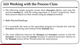
 As with the Thread class, the Process constructor should always be called
using keyword arguments.
 The Process class also provides a similar set of methods to the Thread class
 start() Start the process’s activity. This must be called at most once per
process object. It arranges for the object’s run() method to be invoked in a
separate process.
 join([timeout]) If the optional argument timeout is None (the default),
the method blocks until the joined process terminates. If timeout is a positive
number, it blocks at most timeout seconds. Note that the method returns
None if its process terminates or if the method times out.
 is_alive()Return whether the process is alive. Roughly, a process object is
alive from the moment the start() method returns until the child process
terminates.

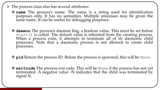
 The process class also has several attributes:
 name The process’s name. The name is a string used for identification
purposes only. It has no semantics. Multiple processes may be given the
same name. It can be useful for debugging purposes.
 daemon The process’s daemon flag, a boolean value. This must be set before
start() is called. The default value is inherited from the creating process.
When a process exits, it attempts to terminate all of its daemonic child
processes. Note that a daemonic process is not allowed to create child
processes.
 pid Return the process ID. Before the process is spawned, this will be None.
 exitcode The process exit code. This will be None if the process has not yet
terminated. A negative value -N indicates that the child was terminated by
signal N.

 In addition to these methods and attributes, the Process class also defines
additional process related methods including
 terminate() Terminate the process.
 kill() Same as terminate() except that on Unix the SIGKILL signal is
used instead of the SIGTERM signal.
 close() Close the Process object, releasing all resources associated with
it. ValueError is raised if the underlying process is still running. Once
close() returns successfully, most of the other methods and attributes of
the Process object will raise a ValueError.

(iii) Working with the Process Class
 The following simple program creates three Process objects; each runs the
function worker(), with the string arguments A, B and C respectively. These
three process objects are then started using the start()method.
 Refer ProcessClassEx.py
 It is essentially the same as the equivalent program for threads but with the
Process class being used instead of the Thread class.
 The main difference between the Thread and Process versions is that the
Process version runs the worker function in separate processes whereas in
the Thread version all the Threads share the same process.

(iv) Alternative Ways to Start a Process
 When the start() method is called on a Process, three different approaches to
starting the underlying process are available.
 These approaches can be set using the multiprocessing.set_start_method()
which takes a string indicating the approach to use.
 The actual process initiation mechanisms available depend on the underlying
operating system:
 ‘spawn’ The parent process starts a fresh Python interpreter process. The child
process will only inherit those resources necessary to run the process objects
run() method. In particular, unnecessary file descriptors and handles from the
parent process will not be inherited. Starting a process using this method is rather
slow compared to using fork or forkserver. Available on Unix and Windows. This
is the default on Windows.

 ‘fork’ The parent process uses os.fork() to fork the Python
interpreter. The child process, when it begins, is effectively identical to the
parent process. All resources of the parent are inherited by the child process.
Available only on Unix type operating systems. This is the default on Unix,
Linux and Mac OS.
 ‘forkserver’ In this case a server process is started. From then on,
whenever a new process is needed, the parent process connects to the server
and requests that it fork a new process. The fork server process is single
threaded, so it is safe for it to use os.fork(). No unnecessary resources are
inherited. Available on Unix style platforms which support passing file
descriptors over Unix pipes.
 The set_start_method()should be used to set the start method (and this
should only be set once within a program).
 Refer SetStartEx.py

 Note that the parent process and current process ids are printed out for the
worker()function, while the main() method prints out only its own id. This
shows that the main application process id is the same as the worker process
parents’ id.
 Alternatively, it is possible to use the get_context() method to obtain a
context object. Context objects have the same API as the multiprocessing
module and allow you to use multiple start methods in the same program, for
example:
ctx = multiprocessing.get_context(‘spawn’)
q = ctx.Queue()
p = ctx.Process(target = foo, args = (q,))

(v) Using a Pool
 Creating Processes is expensive in terms of computer resources. It would
therefore be useful to be able to reuse processes within an application. The
Pool class provides such reusable processes.
 The Pool class represents a pool of worker processes that can be used to
perform a set of concurrent, parallel operations. The Pool provides methods
which allow tasks to be offloaded to these worker processes.
 The Pool class provides a constructor which takes a number of arguments:
class multiprocessing.pool.Pool(processes,
initializer, initargs,
maxtasksperchild,
context)

 These represent:
 processes is the number of worker processes to use. If processes is None
then the number returned by os.cpu_count()is used.
 initializer If initializer is not None then each worker process will
call initializer(*initargs) when it starts.
 maxtasksperchild is the number of tasks a worker process can complete
before it will exit and be replaced with a fresh worker process, to enable
unused resources to be freed. The default maxtasksperchild is None,
which means worker processes will live as long as the pool.
 context can be used to specify the context used for starting the worker
processes. Usually a pool is created using the function multiprocessing.
Pool(). Alternatively the pool can be created using the Pool() method of a
context object.
 The Pool class provides a range of methods that can be used to submit work to
the worker processes managed by the pool. Note that the methods of the Pool
object should only be called by the process which created the pool.

 The following diagram illustrates the effect of submitting some work or task to
the pool.
 From the list of available processes, one process is selected, and the task is
passed to the process.
 The process will then execute the task.
 On completion any results are returned, and the process is returned to the
available list.
 If when a task is submitted to the pool, there are no available processes then the
task will be added to a wait queue until such time as a process is available to
handle the task.

 The simplest of the methods provided by the Pool for work submission is the
map method:
pool.map(func, iterable, chunksize=None)
 This method returns a list of the results obtained by executing the function in
parallel against each of the items in the iterable parameter.
 The func parameter is the callable object to be executed (such as a function
or a method).
 The iteratable is used to pass in any parameters to the function.
 This method chops the iterable into a number of chunks which it submits to
the process pool as separate tasks. The (approximate) size of these chunks
can be specified by setting chunksize to a positive integer. The method
blocks until the result is ready.

 The following sample program illustrates the basic use of the Pool and the
map() method.
 Refer PoolEx.py
 Note that the Pool object must be closed once you have finished with it; we are
therefore using the ‘with as’ statement described earlier in this book to
handle the Pool resource cleanly (it will ensure the Pool is closed when the
block of code within the with as statement is completed).
 As can be seen from this output the map() function is used to run six different
instances of the worker() function with the values provided by the list of
integers. Each instance is executed by a worker process managed by the Pool.

 However, note that the Pool only has 4 worker processes, this means that the
last two instances of the worker function must wait until two of the worker
Processes have finished the work they are doing and can be reused. This can act
as a way of throttling, or controlling, how much work is done in parallel.
 A variant on the map()method is the imap_unordered() method. This
method also applies a given function to an iterable but does not attempt to
maintain the order of the results. The results are accessible via the iterable
returned by the function. This may improve the performance of the resulting
program.
 The following program modified the worker()function to return its result
rather than print it. These results are then accessible by iterating over them as
they are produced via a for loop:

 A further method available on the Pool class is the Pool.apply_async()
method. This method allows operations/functions to be executed
asynchronously allowing the method calls to return immediately.
 That is as soon as the method call is made, control is returned to the calling
code which can continue immediately.
 Any results to be collected from the asynchronous operations can be obtained
either by providing a callback function or by using the blocking get() method
to obtain a result.
 Two examples are shown below, the first uses the blocking get() method. This
method will wait until a result is available before continuing. The second
approach uses a callback function. The callback function is called when a result
is available; the result is passed into the function.
 Refer PoolAsync.py

(vi) Exchanging Data Between Processes
 In some situations, it is necessary for two processes to exchange data.
However, the two process objects do not share memory as they are running in
separate operating system level processes. To get around this the
multiprocessing library provides the Pipe() function.
 The Pipe() function returns a pair of connection.Connection objects
connected by a pipe which by default is duplex (two-way).
 The two connection objects returned by Pipe() represent the two ends of the
pipe. Each connection object has send() and recv() methods (among
others). This allows one process to send data via the send() method of one
end of the connection object. In turn a second process can receive that data via
the receive () method of the other connection object. This is illustrated
below:

 Once a program has finished with a connection is should be closed using
close ().
 The following program illustrates how pipe connections are used:
 Refer DataExchange.py
 Note that data in a pipe may become corrupted if two processes try to read
from or write to the same end of the pipe at the same time. However, there is no
risk of corruption from processes using different ends of the pipe at the same
time.

(vii) Sharing State Between Processes
 In general, if it can be avoided, then you should not share state between
separate processes.
 However, if it is unavoidable then the mutiprocessing library provides two
ways in which state (data) can be shared, these are Shared Memory (as
supported by multiprocessing.Value and multiprocessing.Array)
and Server Process

(a) Process Shared Memory
 Data can be stored in a shared memory map using a
multiprocessing.Value or multiprocessing.Array. This data can be
accessed by multiple processes.
 The constructor for the multiprocessing.Value type is:
multiprocessing.Value (typecode_or_type, *args,
lock = True)
 Where:
 typecode_or_type determines the type of the returned object: it is either
a ctypes type or a one character typecode. For example, ‘d’ indicates a
double precision float and ‘i’ indicates a signed integer.

 *args is passed on to the constructor for the type.
 lock If lock is True (the default) then a new recursive lock object is created
to synchronise access to the value. If lock is False then access to the
returned object will not be automatically protected by a lock, so it will not
necessarily be process-safe.
 The constructor for multiprocessing.Array is
multiprocessing.Array(typecode_or_type,
size_or_initializer,
lock=True)

Where:
 typecode_or_type determines the type of the elements of the returned
array.
 size_or_initializer If size_or_initializer is an integer, then it
determines the length of the array, and the array will be initially zeroed.
Otherwise, size_or_initializer is a sequence which is used to initialise the
array and whose length determines the length of the array.
 If lock is True (the default) then a new lock object is created to synchronise
access to the value. If lock is False then access to the returned object will not
be automatically protected by a lock, so it will not necessarily be “process-
safe”.
 Refer ProcessSharedMemoryEx.py

4. Inter Thread/Process Synchronisation
(i) Introduction
(ii) Using a Barrier
(iii) Event Signalling
(iv) Synchronising Concurrent Code
(v) Python Locks
(vi) Python Conditions
(vii) Python Semaphores
(viii) The Concurrent Queue Class

(i) Introduction
 In this chapter we will look at several facilities supported by both the
threading and multiprocessing libraries that allow for synchronisation and
cooperation between Threads or Processes.
 In the remainder of this chapter we will look at some of the ways in which
Python supports synchronisation between multiple Threads and Processes.
Note that most of the libraries are mirrored between threading and
multiprocessing so that the same basic ideas hold for both approaches with, in
the main, very similar APIs.
 However, you should not mix and match threads and processes. If you are
using Threads, then you should only use facilities from the threading library.
In turn if you are using Processes than you should only use facilities in the
multiprocessing library. The examples given in this chapter will use one or
other of the technologies but are relevant for both approaches.

(ii) Using a Barrier
 Using a threading.Barrier (or multiprocessing.Barrier) is one of
the simplest ways in which the execution of a set of Threads (or Processes) can
be synchronised.
 The threads or processes involved in the barrier are known as the parties that
are taking part in the barrier.
 Each of the parties in the barrier can work independently until it reaches the
barrier point in the code.
 The barrier represents an end point that all parties must reach before any
further behaviour can be triggered.

 At the point that all the parties reach the barrier it is possible to optionally
trigger a post-phase action (also known as the barrier callback).
 This post-phase action represents some behaviour that should be run when all
parties reach the barrier but before allowing those parties to continue.
 The post-phase action (the callback) executes in a single thread (or process).
Once it is completed then all the parties are unblocked and may continue.
 This is illustrated in the following diagram. Threads t1, t2 and t3 are all
involved in the barrier.
 When thread t1 reaches the barrier, it must wait until it is released by the
barrier.

 Similarly, when t2 reaches the barrier, it must wait.
 When t3 finally reaches the barrier, the callback is invoked. Once the callback
has completed the barrier releases all three threads which are then able to
continue.

 An example of using a Barrier object is given below.
 Note that the function being invoked in each Thread must also cooperate in
using the barrier as the code will run up to the barrier.wait() method and
then wait until all other threads have also reached this point before being
allowed to continue.
 The Barrier is a class that can be used to create a barrier object. When the
Barrier class is instantiated, it can be provided with three parameters:
 Where,
 parties the number of individual parties that will participate in the Barrier.
 action is a callable object (such as a function) which, when supplied, will
be called after all the parties have entered the barrier and just prior to
releasing them all.

 timeout If a ‘timeout’ is provided, it is used as the default for all
subsequent wait() calls on the barrier.
 Thus, in the following code
b = Barrier(3, action=callback)
 Indicates that there will be three parties involved in the Barrier and that the
callback function will be invoked when all three reach the barrier (however
the timeout is left as the default value None).
 The Barrier object is created outside of the Threads (or Processes) but must
be made available to the function being executed by the Thread (or Process).
 The easiest way to handle this is to pass the barrier into the function as one of
the parameters; this means that the function can be used with different barrier
objects depending upon the context.

 An example using the Barrier class with a set of Threads is given below:
 Refer BarrierEx.py
 From this you can see that the print_it() function is run three times
concurrently; all three invocations reach the barrier.wait() statement but in a
different order to that in which they were started. Once the three have reached
this point the callback function is executed before the print_it() function
invocations can proceed.
 The Barrier class itself provides several methods used to manage or find out
information about the barrier:

 A Barrier object can be reused any number of times for the same number of
Threads.

 The above example could easily be changed to run using Process by altering
the import statement and creating a set of Processes instead of Threads:
from multiprocessing import Barrier, Process
...
print('Main - Starting')
b = Barrier(3, callback)
t1 = Process(target=print_it, args=('A', b))
 Note that you should only use threads with a threading.Barrier. In turn
you should only use Processes with a multiprocessing.Barrier.

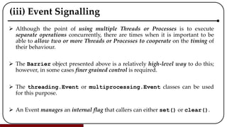
(iii) Event Signalling
 Although the point of using multiple Threads or Processes is to execute
separate operations concurrently, there are times when it is important to be
able to allow two or more Threads or Processes to cooperate on the timing of
their behaviour.
 The Barrier object presented above is a relatively high-level way to do this;
however, in some cases finer grained control is required.
 The threading.Event or multiprocessing.Event classes can be used
for this purpose.
 An Event manages an internal flag that callers can either set() or clear().

 Other threads can wait() for the flag to be set(), effectively blocking their
own progress until allowed to continue by the Event. The internal flag is
initially set to False which ensures that if a task gets to the Event before it is set
then it must wait.
 You can infact invoke wait with an optional timeout. If you do not include the
optional timeout, then wait() will wait forever while wait(timeout)will
wait up to the timeout given in seconds. If the time out is reached, then the wait
method returns False; otherwise wait returns True.
 As an example, the following diagram illustrates two processes sharing an
event object. The first process runs a function that waits for the event to be set.
In turn the second process runs a function that will set the event and thus
release the waiting process.
 Refer EventEx.py

 To change this to use Threads we would merely need to change the import and
to create two Threads:
from threading import Thread, Event
...
print('Starting')
event = Event()
t1 = Thread(target=wait_for_event, args=[event])
t1.start()
t2 = Thread(target=set_event, args=[event])
t2.start()
t1.join()
print('Done')

(iv) Synchronising Concurrent Code
 It is not uncommon to need to ensure that critical regions of code are protected
from concurrent execution by multiple Threads or Processes.
 These blocks of code typically involve the modification of, or access to, shared
data.
 It is therefore necessary to ensure that only one Thread or Process is updating a
shared object at a time and that consumer threads or processes are blocked
while this update is occurring.
 This situation is most common where one or more Threads or Processes are
the producers of data and one or more other Threads or Processes are the
consumers of that data.

 This is illustrated in the following diagram.

 In this diagram the Producer is running in its own Thread (although it could
also run in a separate Process) and places data onto some common shared data
container.
 Subsequently a number of independent Consumers can consume that data
when it is available and when they are free to process the data. However, there
is no point in the consumers repeatedly checking the container for data as that
would be a waste of resources (for example in terms of executing code on a
processor and of context switching between multiple Threads or Processes).
 We therefore need some form of notification or synchronisation between the
Producer and the Consumer to manage this situation.
 Python provides several classes in the threading (and also in the
multiprocessing) library that can be used to manage critical code blocks.
These classes include Lock, Condition and Semaphore.

(v) Python Locks
 The Lock class defined (both in the threading and the multiprocessing
libraries) provides a mechanism for synchronising access to a block of code.
 The Lock object can be in one of two states locked and unlocked (with the
initial state being unlocked).
 The Lock grants access to a single thread at a time; other threads must wait
for the Lock to become free before progressing.
 The Lock class provides two basic methods for acquiring the lock
(acquire()) and releasing (release()) the lock.

 When the state of the Lock object is unlocked, then acquire() changes the
state to locked and returns immediately.
 When the state is locked, acquire() blocks until a call to release() in
another thread changes it to unlocked, then the acquire() call resets it to
locked and returns.
 The release() method should only be called in the locked state; it changes
the state to unlocked and returns immediately. If an attempt is made to
release an unlocked lock, a RuntimeError will be raised.
 An example of using a Lock object is shown below:
 Refer LockEx.py

 The SharedData class presented above uses locks to control access to critical
blocks of code, specifically to the read_value() and the change_value()
methods.
 The Lock object is held internally to the ShareData object and both methods
attempt to acquire the lock before performing their behavior but must then
release the lock after use.
 The read_value() method does this explicitly using try: finally: blocks
while the change_value() method uses a with statement (as the Lock type
supports the Context Manager Protocol). Both approaches achieve the same
result but the with statement style is more concise.
 The SharedData class is used below with two simple functions. In this case
the SharedData object has been defined as a global variable but it could also
have been passed into the reader() and updater() functions as an
argument.

 Both the reader and updater functions loop, attempting to call the
read_value() and change_value() methods on the shared_data object.
 As both methods use a lock to control access to the methods, only one thread
can gain access to the locked area at a time.
 This means that the reader() function may start to read data before the
updater() function has changed the data (or vice versa).
 This is indicated by the output where the reader thread accesses the value ‘0’
twice before the updater records the value ‘1’.
 However, the updater() function runs a second time before the reader gains
access to locked block of code which is why the value 2 is missed. Depending
upon the application this may or may not be an issue.

 Lock objects can only be acquired once; if a thread attempts to acquire a lock
on the same Lock object more than once then a RuntimeError is thrown.
 If it is necessary to re-acquire a lock on a Lock object then the threading.
RLock class should be used.
 This is a Re-entrant Lock and allows the same Thread (or Process) to acquire
a lock multiple times. The code must however release the lock as many times as
it has acquired it.

(vi) Python Conditions
 Conditions can be used to synchronise the interaction between two or more
Threads or Processes.
 Conditions objects support the concept of a notification model; ideal for a
shared data resource being accessed by multiple consumers and producers.
 A Condition can be used to notify one or all of the waiting Threads or
Processes that they can proceed (for example to read data from a shared
resource).

 The methods available that support this are:
 notify() notifies one waiting thread which can then continue
 notify_all() notifies all waiting threads that they can continue
 wait() causes a thread to wait until it has been notified that it can continue
 A Condition is always associated with an internal lock which must be
acquired and released before the wait() and notify() methods can be
called.
 The Condition supports the Context Manager Protocol and can therefore be
used via a with statement (which is the most typical way to use a Condition)
to obtain this lock.

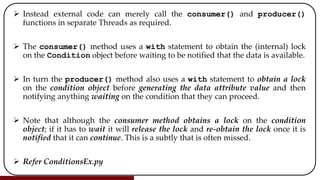
 For example, to obtain the condition lock and call the wait method we might
write:
with condition:
condition.wait()
print('Now we can proceed’)
 The condition object is used in the following example to illustrate how a
producer thread and two consumer threads can cooperate.
 A DataResource class has been defined which will hold an item of data that
will be shared between a consumer and a set of producers.
 It also (internally) defines a Condition attribute. Note that this means that the
Condition is completely internalised to the DataResource class; external
code does not need to know, or be concerned with, the Condition and its use.

 Instead external code can merely call the consumer() and producer()
functions in separate Threads as required.
 The consumer() method uses a with statement to obtain the (internal) lock
on the Condition object before waiting to be notified that the data is available.
 In turn the producer() method also uses a with statement to obtain a lock
on the condition object before generating the data attribute value and then
notifying anything waiting on the condition that they can proceed.
 Note that although the consumer method obtains a lock on the condition
object; if it has to wait it will release the lock and re-obtain the lock once it is
notified that it can continue. This is a subtly that is often missed.
 Refer ConditionsEx.py

(vii) Python Semaphores
 The Python Semaphore class implements Dijkstra’s counting semaphore
model.
 In general, a semaphore is like an integer variable, its value is intended to
represent a number of available resources of some kind.
 There are typically two operations available on a semaphore; these operations
are acquire() and release() (although in some libraries Dijkstra’s original
names of p() and v() are used, these operation names are based on the
original Dutch phrases).

 The acquire() operation subtracts one from the value of the semaphore,
unless the value is 0, in which case it blocks the calling thread until the
semaphore’s value increases above 0 again.
 The signal() operation adds one to the value, indicating a new instance of
the resource has been added to the pool.
 Both the threading.Semaphore and the multiprocessing.Semaphore
classes also supports the Context Management Protocol.
 An optional parameter used with the Semaphore constructor gives the initial
value for the internal counter; it defaults to 1. If the value given is less than 0,
ValueError is raised.
 The following example illustrates 5 different Threads all running the same
worker() function.

 The worker() function attempts to acquire a semaphore; if it does then it
continues into the with statement block; if it doesn’t, it waits until it can
acquire it.
 As the semaphore is initialised to 2 there can only be two threads that can
acquire the Semaphore at a time.
 The sample program however, starts up five threads, this therefore means that
the first 2 running Threads will acquire the semaphore and the remaining thee
will have to wait to acquire the semaphore.
 Once the first two release the semaphore a further two can acquire it and so on.
 Refer SemaphoreEx.py

(viii) The Concurrent Queue Class
 As might be expected the model where a producer Thread or Process
generates data to be processed by one or more Consumer Threads or Processes
is so common that a higher-level abstraction is provided in Python than the
use of Locks, Conditions or Semaphores; this is the blocking queue model
implemented by the threading.Queue or multiprocessing.Queue
classes.
 Both these Queue classes are Thread and Process safe. That is, they work
appropriately (using internal locks) to manage data access from concurrent
Threads or Processes.
 An example of using a Queue to exchange data between a worker process and
the main process is shown below.

 The worker process executes the worker() function sleeping, for 2 s before
putting a string ‘Hello World’ on the queue.
 The main application function sets up the queue and creates the process. The
queue is passed into the process as one of its arguments.
 The process is then started. The main process then waits until data is available
on the queue via the (blocking) get() methods.
 Once the data is available it is retrieved and printed out before the main
process terminates.
 Refer QueueEx.py

 However, this does not make it that clear how the execution of the two
processes interweaves. The following diagram illustrates this graphically:

 In the above diagram the main process waits for a result to be returned from
the queue following the call to the get() method; as it is waiting it is not using
any system resources.
 In turn the worker process sleeps for two seconds before putting some data
onto the queue (via put(‘Hello World’)).
 After this value is sent to the Queue the value is returned to the main process
which is woken up (moved out of the waiting state) and can continue to process
the rest of the main function.

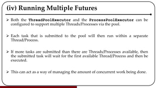
5. Futures
(i) Introduction
(ii) The Need for a Future
(iii) Futures in Python
(a) Future Creation
(b) Simple Example Future
(iv) Running Multiple Futures
(a) Waiting for All Futures to Complete
(b) Processing Results as Completed
(v) Processing Future Results Using a Callback

(i) Introduction
 A future is a thread (or process) that promises to return a value in the future;
once the associated behaviour has completed.
 It is thus a future value.
 It provides a very simple way of firing off behaviour that will either be time
consuming to execute or which may be delayed due to expensive operations
such as Input/Output and which could slow down the execution of other
elements of a program.

(ii) The Need for a Future
 In a normal method or function invocation, the method or function is executed
in line with the invoking code (the caller) having to wait until the function or
method (the callee) returns.
 Only after this the caller able to continue to the next line of code and execute
that.
 In many (most) situations this is exactly what you want as the next line of
code may depend on a result returned from the previous line of code etc.
 However, in some situations the next line of code is independent of the
previous line of code. For example, let us assume that we are populating a
User Interface (UI).

 The first line of code may read the name of the user from some external data
source (such as a database) and then display it within a field in the UI.
 The next line of code may then add today's data to another field in the UI.
 These two lines of code are independent of each other and could be run
concurrently/in parallel with each other.
 In this situation we could use either a Thread or a Process to run the two
lines of code independently of the caller, thus achieving a level of concurrency
and allowing the caller to carry onto the third line of code etc.
 However, neither the Thread or the Process by default provide a simple
mechanism for obtaining a result from such an independent operation.

 This may not be a problem as operations may be self-contained; for example,
they may obtain data from the database or from today’s date and then
updated a UI.
 However, in many situations the calculation will return a result which needs to
be handled by the original invoking code (the caller).
 This could involve performing a long running calculation and then using the
result returned to generate another value or update another object etc.
 A Future is an abstraction that simplifies the definition and execution of such
concurrent tasks.
 Futures are available in many different languages including Python but also
Java, Scala, C++ etc.

 When using a Future; a callable object (such as a function) is passed to the
Future which executes the behaviour either as a separate Thread or as a
separate Process and then can return a result once it is generated.
 The result can either be handled by a call back function (that is invoked when
the result is available) or by using a operation that will wait for a result to be
provided.

(iii) Futures in Python
 The concurrent.futures library was introduced into Python in version 3.2
(and is also available in Python 2.5 onwards). The concurrent.futures
library provides the Future class and a high-level API for working with
Futures.
 The concurrent.futures.Future class encapsulates the asynchronous
execution of a callable object (e.g. a function or method).
 The Future class provides a range of methods that can be used to obtain
information about the state of the future, retrieve results or cancel the future:
 cancel() Attempt to cancel the Future. If the Future is currently being
executed and cannot be cancelled then the method will return False,
otherwise the call will be cancelled and the method will return True.

 cancelled() Returns True if the Future was successfully cancelled.
 running() Returns True if the Future is currently being executed and
cannot be cancelled.
 done() Returns True if the Future was successfully cancelled or finished
running.
 result(timeout=None) Return the value returned by the Future. If the
Future hasn’t yet completed then this method will wait up to timeout
seconds. If the call hasn’t completed in timeout seconds, then a
TimeoutError will be raised. timeout can be an int or float. If timeout is
not specified or None, there is no limit to the wait time. If the future is
cancelled before completing then the CancelledError will be raised. If the
call raised, this method will raise the same exception.
 It should be noted however, that Future instances should not be created
directly, rather they should be created via the submit method of an
appropriate executor.

(a) Future Creation
 Futures are created and executed by Executors. An Executor provides two
methods that can be used to execute a Future (or Futures) and one to shut
down the executor.
 At the root of the executor class hierarchy is the
concurrent.futures.Executor abstract class. It has two subclasses:
 the ThreadPoolExecutor and
 the ProcessPoolExecutor.
 The ThreadPoolExecutor uses threads to execute the futures while the
ProcessPoolExecutor uses separate processes. You can therefore choose
how you want the Future to be executed by specifying one or other of these
executors.

(b) Simple Example Future
 To illustrate these ideas, we will look at a very simple example of using a
Future.
 To do this we will use a simple worker function; similar to that used in the
previous chapters:
 Refer FutureEx.py
 The only difference with this version of worker is that it also returns a result
which is the number of times that the worker printed out the message.

 We can make the invocation of this method into a Future.
 To do this we use a ThreadPoolExecutor imported from the
concurrent.futures module.
 We will then submit the worker function to the pool for execution.
 This returns a reference to a Future which we can use to obtain the result:
 Refer ThreadPoolExecuterEx.py

 Notice how the output from the main program and the worker is interwoven
with two ‘A’s being printed out before the message starting ‘Obtained a…’.
 In this case a new ThreadPoolExecutor is being created with one thread in
the pool (typically there would be multiple threads in the pool but one is being
used here for illustrative purposes).
 The submit() method is then used to submit the function worker with the
parameter ‘A’ to the ThreadPoolExecutor for it to schedule execution of the
function. The submit() method returns a Future object.
 The main program then waits for the future object to return a result (by calling
the result() method on the future). This method can also take a timeout.
 To change this example to use Processes rather than Threads all that is needed
is to change the pool executor to a ProcessPoolExecutor:

 Refer ProcessPoolExecuter.py
 The only difference is that in this particular run the message starting ‘Obtained
a..’ is printed out before any of the ‘A’s are printed; this may be due to the fact
that a Process initially takes longer to set up than a Thread.

(iv) Running Multiple Futures
 Both the ThreadPoolExecutor and the ProcessPoolExecutor can be
configured to support multiple Threads/Processes via the pool.
 Each task that is submitted to the pool will then run within a separate
Thread/Process.
 If more tasks are submitted than there are Threads/Processes available, then
the submitted task will wait for the first available Thread/Process and then be
executed.
 This can act as a way of managing the amount of concurrent work being done.

 For example, in the following example, the worker() function is submitted to the pool
four times, but the pool is configured to use threads. Thus the fourth worker will need
to wait until one of the first three completes before it is able to execute:
 Refer MultipleFuturesEx.py
 When this runs we can see that the Futures for A, B and C all run concurrently but D
must wait until one of the others finishes:
 The main thread also waits for future4 to finish as it requests the result which is a
blocking call that will only return once the future has completed and generates a result.
 Again, to use Processes rather than Threads all we need to do is to replace the
ThreadPoolExecutor with the ProcessPoolExecutor:
 Refer MultipleFuturesEx1.py

(a) Waiting for All Futures to Complete
 It is possible to wait for all futures to complete before progressing.
 In the previous section it was assumed that future4 would be the last future to
complete; but in many cases it may not be possible to know which future will
be the last to complete.
 In such situations it is very useful to be able to wait for all the futures to
complete before continuing.
 This can be done using the concurrent.futures.wait function. This
function takes a collection of futures and optionally a timeout and a
return_when indicator.

wait(fs, timeout=None, return_when=ALL_COMPLETED)
 where:
 timeout can be used to control the maximum number of seconds to wait
before returning. timeout can be an int or float. If timeout is not specified or
None, there is no limit to the wait time.
 return_when indicates when this function should return. It must be one of the
following constants:
 FIRST_COMPLETED The function will return when any future finishes or
is cancelled.
 FIRST_EXCEPTION The function will return when any future finishes by
raising an exception. If no future raises an exception, then it is equivalent to
ALL_COMPLETED.
 ALL_COMPLETED The function will return when all futures finish or are
cancelled.

 The wait() function returns two sets done and not_done. The first set
contains the futures that completed (finished or were cancelled) before the wait
completed. The second set, the not_dones, contains uncompleted futures.
 We can use the wait() function to modify out previous example so that we no
longer rely on future4 finishing last:
 Refer FutureWaitEx.py
 Note how each future is added to the list of futures which is then passed to the
wait() function.

(b) Waiting for All Futures to Complete
 What if we want to process each of the results returned by our collection of futures?
 We could loop through the futures list in the previous section once all the results have
been generated. However, this means that we would have to wait for them all to
complete before processing the list.
 In many situations we would like to process the results as soon as they are generated
without being concerned if that is the first, third, last or second etc.
 The concurrent.futures.as_completed() function does preciously this; it will
serve up each future in turn as soon as they are completed; with all futures eventually
being returned but without guaranteeing the order (just that as soon as a future is
finished generating a result it will be immediately available).

 For example, in the following example, the is_even() function sleeps for a
random number of seconds (ensuring that different invocations of this function
will take different durations) then calculates a result:
 Refer AsCompletedEx.py
 As you can see from this output although the six futures were started in
sequence the results returned are in a different order (with the returned order
being 1, 4, 5, 3, 2 and finally 6).

(v) Processing Future Results Using a Callback
 An alternative to the as_complete() approach is to provide a function that will
be called once a result has been generated. This has the advantage that the
main program is never paused; it can continue doing whatever is required of
it.
 The function called once the result is generated is typically known as a
callback function; that is the future calls back to this function when the result
is available.
 Each future can have a separate call back as the function to invoke is set on the
future using the add_done_callback() method. This method takes the name of
the function to invoke.

 For example, in this modified version of the previous example, we specify a
callback function that will be used to print the futures result. This call back
function is called print_future_result(). It takes the future that has completed as
its argument:
 Refer FutureResultEx.py
 When we run this, we can see that the call back function is called after the main
thread has completed. Again, the order is unspecified as the is_even()
function still sleeps for a random amount of time.

6. Concurrency with AsyncIO
(i) Introduction
(ii) Asynchronous IO
(iii) Async IO Event Loop
(iv) The Async and Await Keywords
(a) Using Async and Await
(v) Async IO Tasks
(vi) Running Multiple Tasks
(a) Collating Results from Multiple Tasks
(b) Handling Task Results as They Are Made Available

(i) Introduction
 The Async IO facilities in Python are relatively recent additions originally
introduced in Python 3.4 and evolving up to and including Python 3.7.
 They are comprised (as of Python 3.7) of two new keywords async and
await (introduced in Python 3.7) and the Async IO Python package.

(ii) Asynchronous IO
 Asynchronous IO (or Async IO) is a language agnostic concurrent
programming model (or paradigm) that has been implemented in several
different programming language (such as C# and Scala) as well as in Python.
 Asynchronous IO is another way in which you can build concurrent
applications in Python.
 It is in many ways an alternative to the facilities provided by the Threading
library in Python.
 However, were as the Threading library is more susceptible to issues
associated with the GIL (The Global Interpreter Lock) which can affect
performance, the Async IO facilities are better insulated from this issue

 The way in which Async IO operates is also lighter weight then the facilities
provide day the multiprocessing library since the asynchronous tasks in Async
IO run within a single process rather than requiring separate processes to be
spawned on the underlying hardware.
 Async IO is therefore another alternative way of implementing concurrent
solutions to problems.
 It should be noted that it does not build on either Threading or Multi -
Processing; instead Async IO is based on the idea of cooperative multitasking.
 These cooperating tasks operate asynchronously; by this we mean that the
tasks:
 are able to operate separately from other tasks,
 are able to wait for another task to return a result when required,
 and are thus able to allow other tasks to run while they are waiting.

 The IO (Input/Output) aspect of the name Async IO is because this form of
concurrent program is best suited to I/O bound tasks.
 In an I/O bound task a program spends most of its time sending data to, or
reading data from, some form of external device (for example a database or set
of files etc.).
 This communication is time consuming and means that the program spends
most of its time waiting for a response from the external device.
 One way in which such I/O bound applications can (appear to) speed up is to
overlap the execution of different tasks; thus, while one task is waiting for a
database to respond with some data, another task can be writing data to a log
file etc.

(iii) Async IO Event Loop
 When you are developing code using the Async IO facilities you do not need
to worry about how the internals of the Async IO library work; however at
least at the conceptual level it is useful to understand one key concept; that of
the Async IO Event Loop; This loop controls how and when each task gets run.
For the purposes of this discussion a task represents some work that can be
run independently of other pieces of work.
 The Event Loop knows about each task to be run and what the state of the task
currently is (for example whether it is waiting for something to
happen/complete).
 It selects a task that is ready to run from the list of available tasks and executes
it.

 This task has complete control of the CPU until it either completes its work or
hands back control to the Event Loop (for example, because it must now wait
for some data to be supplied from a database).
 The Event Loop now checks to see if any of the waiting tasks are ready to
continue executing and makes a note of their status.
 The Event Loop then selects another task that is ready to run and starts that
task off. This loop continues until all the tasks have finished.

 An important point to note in the above description is that a task does not give
up the processor unless it decides to, for example by having to wait for
something else.
 They never get interrupted in the middle of an operation; this avoids the
problem that two threads might have when being time sliced by a separate
scheduler as they may both be sharing the same resource. This can greatly
simplify your code.

(iv) The Async and Await Keywords
 The async keyword, introduced in Python 3.7 is used to mark a function as
being something that uses the await keyword (we will come back to this
below as there is one other use of the async keyword).
 A function that uses the await keyword can be run as a separate task and can
give up control of the processor when it calls await against another async
function and must wait for that function to complete.
 The invoked async function can then run as a separate task etc.
 To invoke an async function it is necessary to start the Async IO Event Loop
and for that function to be treated as a task by the Event Loop. This is done by
calling the asyncio.run() method and passing in the root async function.

 The asyncio.run() function was introduced in Python 3.7 (older versions of
Python such as Python 3.6 required you to explicitly obtain a reference to the
Event Loop and to run the root async function via that).
 One point to note about this function is that it has been marked as being
provisional in Python 3.7.
 This means that future versions of Python may or may not support the function
or may modify the function in some way.
 You should therefore check the documentation for the version of Python you
are using to see whether the run method has been altered or not.

(a) Using Async and Await
 The main() function is the entry point for the program and calls:
asyncio.run(do_something())
 This starts the Async IO Event Loop running and results in the
do_something()function being wrapped up in a Task that is managed by
the loop.
 Note that you do not explicitly create a Task in Async IO; they are always
created by some function however it is useful to be aware of Tasks as you can
interact with them to check their status or to retrieve a result.
 The do_something()function is marked with the keyword async.

 As previously mentioned, this indicates that it can be run as a separate Task
and that it can use the keyword await to wait for some other function or
behaviour to complete.
 In this case the do_something() asynchronous function must wait for the
worker() function to complete.
 The await keyword does more than merely indicate that the do_something()
function must wait for the worker to complete.
 It triggers another Task to be created that will execute the worker() function
and releases the processor allowing the Event Loop to select the next task to
execute (which may or may not be the task running the worker() function).
 The status of the do_something task is now waiting while the status of the
worker() task is ready (to run).

 The async keyword again indicates that this function can be run as a separate task.
 However, this time the body of the function does not use the await keyword. This is
because this is a special case known as an Async IO coroutine function.
 This is a function that returns a value from a Task (it is related to the idea of a standard
Python coroutine which is a data consumer).
 Refer AsyncWaitEx.py
 When this is run there is a pause between the two worker printouts as it sleeps.
Although it is not completely obvious here, the do_something() function was run as
one task, this task then waited when it got to the worker() function which was run as
another Task. Once the worker task completed the do_something task could continue
and complete its operation. Once this happened the Async IO Event Loop could then
terminate as no further tasks were available.

(v) Async IO Tasks
 Tasks are used to execute functions marked with the async keyword
concurrently.
 Tasks are never created directly instead they are created implicitly via the
keyword await or through functions such as asyncio.run described above
or asyncio.create_task(), asyncio.gather()and
asyncio.as_completed().

 These additional task creation functions are described below:
 asyncio.create_task() This function takes a function marked with
async and wraps it inside a Task and schedules it for execution by the Async
IO Event Loop. This function was added in Python 3.7.
 asyncio.gather(*aws) This function runs all the async functions passed
to it as separate Tasks. It gathers the results of each separate task together
and returns them as a list. The order of the results corresponds to the order
of the async functions in the aws list.
 asyncio.as_completed(aws) Runs each of the async functions passed to
it.

 A Task object supports several useful methods
 cancel() cancels a running task. Calling this method will cause the Task to
throw a CancelledError exception.
 cancelled() returns True if the Task has been cancelled.
 done()returns True if the task has completed, raised an exception or was
cancelled.
 result() returns the result of the Task if it is done. If the Tasks result is not
yet available, then the method raises the InvalidStateError exception.
 exception()return an exception if one was raised by the Task. If the task
was cancelled then raises the CancelledError exception. If the task is not
yet done, then raises an InvalidStateError exception.

 It is also possible to add a callback function to invoke once the task has
completed (or to remove such a function if it has been added):
 add_done_callback(callback) Add a callback to be run when the Task
is done.
 remove_done_callback(callback) Remove callback from the callbacks
list.
 Note that the method is called ‘add’ rather than ‘set’ implying that there can be
multiple functions called when the task has completed (if required).
 In this example, the worker() function is wrapped within a task object that is
returned from the asyncio.create_task(worker()) call.
 A function (print_it())is registered as a callback on the task using the
asyncio.create_task(worker()) function.

 Note that the worker is passed the task that has completed as a parameter. This
allows it to obtain information from the task such as any result generated.
 In this example the async function do_something() explicitly waits on the
task to complete. Once this happens several different methods are used to
obtain information about the task (such as whether it was cancelled or not).
 One other point to note about this listing is that in the worker() function we
have added an await using the asyncio.sleep(1)function; this allows the
worker to sleep and wait for the triggered task to complete; it is an Async IO
alternative to time.sleep(1).
 Refer AsyncIOTasksEx.py

(vi) Running Multiple Tasks
 In many cases it is useful to be able to run several tasks concurrently. There are
two options provided for this the asyncio.gather() and the
asyncio.as_completed() function.

(a) Collating Results from Multiple Tasks
 It is often useful to collect all the results from a set of tasks together and to
continue only once all the results have been obtained.
 When using Threads or Processes this can be achieved by starting multiple
Threads or Processes and then using some other object such as a Barrier to
wait for all the results to be available before continuing.
 Within the Async IO library all that is required is to use the asyncio.gather()
function with a list of the async functions to run, for example:
 Refer CollatingResults.py

(b) Handling Task Results as They Are Made Available
 Another option when running multiple Tasks is to handle the results as they
become available, rather than wait for all the results to be provided before
continuing.
 This option is supported by the asyncio.as_completed() function. This function
returns an iterator of async functions which will be served up as soon as they
have completed their work.
 The for-loop construct can be used with the iterator returned by the function;
however within the for loop the code must call await on the async functions
returned so that the result of the task can be obtained.
 Refer HandlingTasksEx.py

 As you can see from this, the results are not returned in the order that the tasks
are created, task ‘C’ completes first followed by ‘A’ and ‘B’.
 This illustrates the behaviour of the asyncio.as_completed() function.

1. Reactive Programming Introduction
2. RxPy Observables, Observers and Subjects
3. RxPy Operators
ASYNCHRONOUS PROGRAMMING

1. Reactive Programming Introduction
(i) Introduction
(ii) What Is a Reactive Application?
(iii)The ReactiveX Project
(iv) The Observer Pattern
(v) Hot and Cold Observables
(a) Cold Observables
(b) Hot Observables
(c) Implications of Hot and Cold Observables
(vi) Differences Between Event Driven Programming and Reactive Programming
(vii) Advantages of Reactive Programming
(viii) Disadvantages of Reactive Programming
(ix) The RxPy Reactive Programming Framework

(i) Introduction
 Reactive programming is a way of write programs that allow the system to
reactive to data being published to it.
 We will look at the RxPy library which provides a Python implementation of
the ReactiveX approach to Reactive Programming.

(ii) What Is a Reactive Application?
 A Reactive Application is one that must react to data; typically, either to the presence
of new data, or to changes in existing data. The Reactive Manifesto presents the key
characteristics of Reactive Systems as:
 Responsive. This means that such systems respond in a timely manner. Here
ofcourse timely will differ depending upon the application and domain; in one
situation a second may be timely in another it may be far too slow.
 Resilient. Such systems stay responsive in the face of failure. The systems must
therefore be designed to handle failure gracefully and continue to work
appropriately following the failure.
 Elastic. As the workload grows the system should continue to be responsive.
 Message Driven. Information is exchanged between elements of a reactive system
using messages. This ensures loose coupling, isolation and location transparency
between these components.

 As an example, consider an application that lists a set of Equity Stock Trade
values based on the latest market stock price data.
 This application might present the current value of each trade within a table.
When new market stock price data is published, then the application must
update the value of the trade within the table. Such an application can be
described as being reactive.
 Reactive Programming is a programming style (typically supported by
libraries) that allows code to be written that follow the ideas of reactive
systems.
 Of course, just because part of an application uses a Reactive Programming
library does not make the whole application reactive; indeed, it may only be
necessary for part of an application to exhibit reactive behaviour.

(iii) The ReactiveX Project
 ReactiveX is the best-known implementation of the Reactive Programming
paradigm.
 ReactiveX is based on the Observer-Observable design pattern.
 However, it is an extension to this design pattern as it extends the pattern such
that the approach supports sequences of data and/or events and adds
operators that allow developers to compose sequences together declaratively
while abstracting away concerns associated with low-level threads,
synchronisation, concurrent data structures and non-blocking I/O.

 The ReactiveX project has implementations for many languages including
RxJava, RxScala and RxPy; this last is the version we are looking at as it is for
the Python language.
 RxPy is described as: A library for composing asynchronous and event-based
programs using Observable collections and query operator functions in
Python.

(iv) The Observer Pattern
 The Observer Pattern is one of the Gang of Four set of Design Patterns. The
Gang of Four Patterns (as originally described in Gamma et al. 1995) are so
called because this book on design patterns was written by four very famous
authors namely; Erich Gamma, Richard Helm, Ralph Johnson and John
Vlissides.
 The Observer Pattern provides a way of ensuring that a set of objects is
notified whenever the state of another object changes. It has been widely used
in a number of languages (such as Smalltalk and Java) and can also be used
with Python.
 The intent of the Observer Pattern is to manage a one-to-many relationship
between an object and those objects interested in the state, and in particular
state changes, of that object.

 Thus, when the objects’ state changes, the interested (dependent) objects are
notified of that change and can take whatever action is appropriate.
 There are two key roles within the Observer Pattern, these are the Observable
and the Observer roles.
 Observable. This is the object that is responsible for notifying other objects
that a change in its state has occurred.
 Observer. An Observer is an object that will be notified of the change in state
of the Observable and can take appropriate action (such as triggering a
change in their own state or performing some action).
 In addition, the state is typically represented explicitly:
 State. This role may be played by an object that is used to share information
about the change in state that has occurred within the Observable. This
might be as simple as a String indicating the new state of the Observable or it
might be a data-oriented object that provides more detailed information.

 These roles are illustrated in the following figure.
 In the above figure, the Observable object publishes data to a Data Stream. The
data in the Data Stream is then sent to each of the Observers registered with the
Observable. In this way data is broadcast to all Observers of an Observable.
 It is common for an Observable to only publish data once there is an Observer
available to process that data.

 The process of registering with an Observable is referred to as subscribing.
Thus, an Observable will have zero or more subscribers (Observers).
 If the Observable publishes data at a faster rate than can be processed by the
Observer, then the data is queued via the Data Stream.
 This allows the Observer to process the data received one at a time at its own
pace; without any concern for data loss (as long as sufficient memory is
available for the data stream).

(v) Hot and Cold Observables
 Another concept that it is useful to understand is that of Hot and Cold
Observables.
 Cold Observables are lazy Observables. That is, a Cold Observable will only
publish data if at least one Observer is subscribed to it.
 Hot Observables, by contrast, publish data whether there is an Observer
subscribed or not.

(a) Cold Observables
 A Cold Observable will not publish any data unless there is at least one
Observer subscribed to process that data.
 In addition, a cold Observable only provides data to an Observer when that
Observer is ready to process the data; this is because the Observable-Observer
relationship is more of a pull relationship.
 For example, given an Observable that will generate a set of values based on a
range, then that Observable will generate each result lazily when requested by
an Observer.
 If the Observer takes some time to process the data emitted by the Observable,
then the Observable will wait until the Observer is ready to process the data
before emitting another value.

(b) Hot Observables
 Hot Observables by contrast publish data whether there is an Observer
subscribed or not.
 When an Observer registers with the Observable, it will start to receive data at
that point, as and when the Observable publishes new data.
 If the Observable has already published previous data items, then these will
have been lost and the Observer will not receive that data.
 The most common situation in which a Hot Observable is created is when the
source producer represents data that may be irrelevant if not processed
immediately or may be superseded by subsequent data.

 For example, data published by a Stock Market Price data feed would fall into
this category.
 When an Observable wraps around this data feed it can publish that data
whether or not an Observer is subscribed.

(c) Implications of Hot and Cold Observables
 It is important to know whether you have a hot or cold Observable because
this can impact on what you can assume about the data supplied to the
Observers and thus how you need to design your application.
 If it is important that no data is lost, then care is needed to ensure that the
subscribers are in place before a Hot Observable starts to publish data
(whereas this is not a concern for a cold Observable).

(vi) Differences Between Event Driven Programming and Reactive
Programming
 In Event Driven programming, an event is generated in response too
something happening; the event then represents this with any associated data.
 For example, if the user clicks the mouse then an associated
MouseClickEvent might be generated. This object will usually hold
information about the x and y coordinates of the mouse along with which
button was clicked etc.
 It is then possible to associate some behaviour (such as a function or a
method) with this event so that if the event occurs, then the associated
operation is invoked and the event object is provided as a parameter.
 This is certainly the approach used in the wxPython library presented earlier
in this book:

 From the above diagram, when a MoveEvent is generated the on_move()
method is called, and the event is passed into the method.
 In the Reactive Programming approach, an Observer is associated with an
Observable. Any data generated by the Observable will be received and
handled by the Observer.
 This is true whatever that data is, as the Observer is a handler of data generated
by the Observable rather than a handler of a specific type of data (as with the
Event driven approach).

 Both approaches could be used in many situations. For example, we could have
a scenario in which some data is to be processed whenever a stock price
changes.
 This could be implemented using a StockPriceChangeEvent associated
with a StockPriceEventHandler. It could also be implemented via Stock
PriceChangeObserverable and a StockPriceChangeObserver.
 In either case one element handles the data generated by another element.
 However, the RxPy library simplifies this process and allows the Observer to
run in the same thread as, or a separate thread from, the Observable with just a
small change to the code.

(vii) Advantages of Reactive Programming
 There are several advantages to the use of a Reactive Programming library
these include:
 It avoids multiple callback methods. The problems associated with the use
of callbacks are sometimes referred to as callback hell. This can occur when
there are multiple callbacks, all defined to run in response to some data
being generated or some operation completing. It can be hard to
understand, maintain and debug such systems.
 Simpler asynchronous, multi threaded execution. The approach adopted by
RxPy makes it very easy to execute operations/ behaviour within a
multithreaded environment with independent asynchronous functions.

 Available Operators. The RxPy library comes pre built with numerous
operators that make processing the data produced by an Observable much
easier.
 Data Composition. It is straight forward to compose new data streams
(Observables) from data supplied by two or more other Observables for
asynchronous processing.

(viii) Disadvantages of Reactive Programming
 Its easy to over complicate things when you start to chain operators together.
If you use too many operators, or too complex a set of functions with the
operators, it can become hard to understand what is going on.
 Many developers think that Reactive programming is inherently multi-
threaded; this is not necessarily the case; in fact, RxPy (the library explored in
the next two chapters) is single threaded by default. If an application needs the
behaviour to execute asynchronously then it is necessary to explicitly indicate
this.
 Another issue for some Reactive programming frameworks is that it can
become memory intensive to store streams of data so that Observers can
processes that data when they are ready.

(ix) The RxPy Reactive Programming Framework
 The RxPy library is a part of the larger ReactiveX project and provides an
implementation of ReactiveX for Python.
 It is built on the concepts of Observables, Observers, Subjects and operators.

2. RxPy Observables, Observers and Subjects
(i) Introduction
(ii) Observables in RxPy
(iii) Observers in RxPy
(iv) Multiple Subscribers/Observers
(v) Subjects in RxPy
(vi) Observer Concurrency
(a) Available Schedulers

(i) Introduction
 In this chapter we will discuss Observables, Observers and Subjects.
 We also consider how observers may or may not run concurrently.
 In the remainder of this chapter we look at RxPy version 3 which is a major
update from RxPy version 1.

(ii) Observables in RxPy
 An Observable is a Python class that publishes data so that it can be
processed by one or more Observers (potentially running in separate threads).
 An Observable can be created to publish data from static data or from
dynamic sources.
 Observables can be chained together to control how and when data is
published, to transform data before it is published and to restrict what data is
actually published.

 For example, to create an Observable from a list of values we can use the
rx.from_list() function. This function (also known as an RxPy operator)
is used to create the new Observable object:
import rx
Observable = rx.from_list([2, 3, 5, 7])

(iii) Observers in RxPy
 We can add an Observer to an Observable using the subcribe() method.
 This method can be supplied with a lambda function, a named function or an
object whose class implements the Observer protocol.
 For example, the simplest way to create an Observer is to use a lambda
function:
# Subscribe a lambda function
observable.subscribe(lambda value: print('Lambda Received',value))

 When the Observable publishes data the lambda function will be invoked.
 Each data item published will be supplied independently to the function. The
output from the above subscription for the previous Observable is:
Lambda Received 2
Lambda Received 3
Lambda Received 5
Lambda Received 7
 We can also have used a standard or named function as an Observer:
def prime_number_reporter(value):
print('Function Received', value)
# Subscribe a named function
observable.subscribe(prime_number_reporter)

 Note that it is only the name of the function that is used with the
subscribe() method (as this effectively passes a reference to the function into
the method).
 If we now run this code using the previous Observable we get:
Function Received 2
Function Received 3
Function Received 5
Function Received 7

 In actual fact the subscribe() method takes four optional parameters. These
are:
 on_next Action to invoke for each data item generated by the Observable.
 on_error Action to invoke upon exceptional termination of the Observable
sequence.
 on_completed Action to invoke upon graceful termination of the
Observable sequence.
 Observer The object that is to receive notifications. You may subscribe
using an Observer or callbacks, not both.
 Each of the above can be used as positional parameters or as keyword
arguments, for example:

# Use lambdas to set up all three functions
observable.subscribe(
on_next = lambda value: print('Received on_next', value),
on_error = lambda exp: print('Error Occurred', exp),
on_completed = lambda: print('Received completed notification’)
)
 The above code defines three lambda functions that will be called depending upon whether
data is supplied by the Observable, if an error occurs or when the data stream is terminated.
The output from this is:
Received on_next 2
Received on_next 3
Received on_next 5
Received on_next 7
Received completed notification

 Note that the on_error function is not run as no error was generated in this example.
 The final optional parameter to the subscribe() method is an Observer object. An Observer
object can implement the Observer protocol which has the following methods on_next(),
on_completed() and on_error(), for example:
class PrimeNumberObserver:
def on_next(self, value):
print('Object Received', value)
def on_completed(self):
print('Data Stream Completed')
def on_error(self, error):
print('Error Occurred', error)
 Instances of this class can now be used as an Observer via the subscribe() method:
# Subscribe an Observer object
observable.subscribe(PrimeNumberObserver())

 The output from this example using the previous Observable is:
Object Received 2
Object Received 3
Object Received 5
Object Received 7
Data Stream Completed
 Note that the on_completed() method is also called; however the on_errror() method is
not called as there were no exceptions generated.
 The Observer class must ensure that the methods implemented adhere to the Observer protocol
(i.e. That the signatures of the on_next(), on_completed () and on_error() methods
are correct).

(iv) Multiple Subscribers/Observers
 An Observable can have multiple Observers subscribed to it.
 In this case each of the Observers is sent all of the data published by the
Observable.
 Multiple Observers can be registered with an Observable by calling the
subscribe method multiple times.
 For example, the following program has four subscribers as well as on_error
and on_completed function registered:
 Refer SubscriberObserverEx.py

(v) Subjects in RxPy
 A subject is both an Observer and an Observable. This allows a subject to
receive an item of data and then to republish that data or data derived from it.
 For example, imagine a subject that receives stock market price data
published by an external (to the organisation receiving the data) source. This
subject might add a timestamp and source location to the data before
republishing it to other internal Observers.
 However, there is a subtle difference that should be noted between a Subject
and a plain Observable. A subscription to an Observable will cause an
independent execution of the Observable when data is published.

 Notice how in the previous section all the messages were sent to a specific
Observer before the next Observer was sent any data at all.
 However, a Subject shares the publication action with all of the subscribers and
they will therefore all receive the same data item in a chain before the next data
item.
 In the class hierarchy the Subject class is a direct subclass of the Observer
class.
 The following example creates a Subject that enriches the data it receives by
adding a timestamp to each data item. It then republishes the data item to any
Observers that have subscribed to it.
 Refer SubjectEx.py

(vi) Observer Concurrency
 By default, RxPy uses a single threaded model; that is Observables and
Observers execute in the same thread of execution. However, this is only the
default as it is the simplest approach.
 It is possible to indicate that when a Observer subscribes to an Observable that
it should run in a separate thread using the scheduler keyword parameter on
the subscribe() method.
 This keyword is given an appropriate scheduler such as the
rx.concurrency.NewThreadScheduler.
 This scheduler will ensure that the Observer runs in a separate thread.

 To see the difference look at the following two programs. The main difference between
the programs is the use of specific schedulers:
import rx
Observable = rx.from_list([2, 3, 5])
observable.subscribe(lambda v: print('Lambda1 Received', v))
Output:
Lambda1 Received 2
Lambda1 Received 3
Lambda1 Received 5
Lambda2 Received 2
Lambda2 Received 3
Lambda2 Received 5
Lambda3 Received 2
Lambda3 Received 3
Lambda3 Received 5

 The subscribe() method takes an optional keyword parameter called
scheduler that allows a scheduler object to be provided.
 Now if we specify a few different schedulers, we will see that the effect is to run
the Observers concurrently with the resulting output being interwoven:
 Refer ConcurrentObserversEx.py

(a) Available Schedulers
 To support different scheduling strategies the RxPy library provides two
modules that supply different schedulers; the rx.concurrency and
rx.currency.mainloopscheduler. The modules contain a variety of
schedulers including those listed below.
 The following schedulers are available in the rx.concurrency module:
 ImmediateScheduler This schedules an action for immediate execution.
 CurrentThreadScheduler This schedules activity for the current thread.
 TimeoutScheduler This scheduler works via a timed callback.
 NewThreadScheduler creates a scheduler for each unit of work on a
separate thread.
 ThreadPoolScheduler This is a scheduler that utilises a thread pool to
execute work. This scheduler can act as a way of throttling the amount of
work carried out concurrently.

 The rx.concurrency.mainloopscheduler module also defines the
following schedulers:
 IOLoopScheduler A scheduler that schedules work via the Tornado I/O main
event loop.
 PyGameScheduler A scheduler that schedules works for PyGame.
 WxScheduler A scheduler for a wxPython event loop.

3. RxPy Operators
(i) Introduction
(ii) Reactive Programming Operators
(iii) Piping Operators
(iv) Creational Operators
(v) Transformational Operators
(vi) Combinatorial Operators
(vii)Filtering Operators
(viii)Mathematical Operators
(ix) Chaining Operators

(i) Introduction
 There are different types of operators provided by RxPy that can be applied to
the data emitted by an Observable

(ii) Reactive Programming Operators
 Behind the interaction between an Observable and an Observer is a data
stream. That is the Observable supplies a data stream to an Observer that
consumes/ processes that stream.
 It is possible to apply an operator to this data stream that can be used to to
filter, transform and generally refine how and when the data is supplied to the
Observer.
 The operators are mostly defined in the rx.operators module, for example
rx.operators.average(). However it is common to use an alias for this
such that the operators module is called op, such as
from rx import operators as op

 This allows for a short hand form to be used when referencing an operator,
such as op.average().
 Many of the RxPy operators execute a function which is applied to each of the
data items produced by an Observable.
 Others can be used to create an initial Observable (indeed you have already
seen these operators in the form of the from_list() operator).
 Another set of operators can be used to generate a result based on data
produced by the Observable (such as the sum() operator).

 In fact, RxPy provides a wide variety of operators, and these operators can be
categorised as follows:
 Creational,
 Transformational,
 Combinatorial,
 Filters,
 Error handlers,
 Conditional and Boolean operators,
 Mathematical,
 Connectable.

(iii) Piping Operators
 To apply an operator other than a creational operator to an Observable it is
necessary to create a pipe.
 A Pipe is essentially a series of one or more operations that can be applied to
the data stream generated by the Observable.
 The result of applying the pipe is that a new data stream is generated that
represents the results produced following the application of each operator in
turn.

 To create a pipe the Observable.pipe() method is used.
 This method takes a comma delimited list of one or more operators and returns
a data stream.
 Observers can then subscribe to the pipe’s data stream.

(iv) Creational Operators
 The rx.from_list() operator is an example of a creational operator. It is
used to create a new Observable based on data held in a list like structure.
 A more generic version of from_list() is the from_() operator.
 This operator takes an iterable and generates an Observable based on the data
provided by the iterable.
 Any object that implements the iterable protocol can be used including user
defined types. There is also an operator from_iterable().
 All three operators do the same thing and you can choose which to use based
on which provides the most semantic meaning in your context.

 All three of the following statements have the same effect:
source = rx.from_([2, 3, 5, 7])
source = rx.from_iterable([2, 3, 5, 7])
source = rx.from_list([2, 3, 5, 7])
 This is illustrated pictorially below:

 Another creational operator is the rx.range() operator. This operator
generates an observable for a range of integer numbers.
 The range can be specified with or without a starting value and with or within
an increment. However, the maximum value in the range must always be
provided, for example:
obs1 = rx.range(10)
obs2 = rx.range(0, 10)
obs3 = rx.range(0, 10, 1)

(v) Transformational Operators
 There are several transformational operators defined in the rx.operators
module including rx.operators.map() and rx.operators.flat_map().
 The rx.operators.map() operator applies a function to each data item
generated by an Observable.
 The rx.operators.flat_map() operator also applies a function to each data
item but then applies a flatten operation to the result. For example, if the result is
a list of lists then flat_map will flatten this into a single list.

 The rx.operators.map() operator allows a function to be applied to all data
items generated by an Observable. The result of this function is then returned
as the result of the map() operators Observable.
 The function is typically used to perform some form of transformation to the
data supplied to it.
 This could be adding one to all integer values, converting the format of the data
from XML to JSON, enriching the data with additional information such as the
time the data was acquired and who the data was supplied by etc.
 In the example given below we are transforming the set of integer values
supplied by the original Observable into strings.

 In the diagram these strings include quotes around them to highlight they are
in fact a string:
 This is typical of the use of a transformation operator; that is to change the data
from one format to another or to add information to the data.
 The code used to implement this scenario is given below. Note the use of the
pipe() method to apply the operator to the data stream generated by the
Observable:

# Apply a transformation to a data source to convert integers into strings
import rx
# Set up a source with a map function
source = rx.from_list([2, 3, 5, 7]).pipe(op.map(lambda value:
"'" + str(value) + “’”))
source.subscribe(lambda value: print('Lambda Received’,
value,' is a string ‘,
isinstance(value, str)))

The output from this program is:
Lambda Received '2' is a string True

(vi) Combinatorial Operators
 Combinatorial operators combine together multiple data items in some way.
One example of a combinatorial operator is the rx.merge() operator. This
operator merges the data produced by two Observables into a single Observable
data stream.
 For example:

 In the above diagram two Observables are represented by the sequence 2, 3, 5, 7 and the
sequence 11, 13, 16, 19.
 These Observables are supplied to the merge operator that generates a single
Observable that will supply data generated from both of the original Observables. This
is an example of an operator that does not take a function but instead takes two
Observables.
 The code representing the above scenario is given below:
# An example illustrating how to merge two data sources
import rx
# Set up two sources
source1 = rx.from_list([2, 3, 5, 7])
source2 = rx.from_list([10, 11, 12])
# Merge two sources into one
rx.merge(source1, source2).
subscribe(lambda v: print(v, end=','))

 Notice that in this case we have subscribed directly to the Observable returned
by the merge() operator and have not stored this in an intermediate variable
(this was a design decision and either approach is acceptable).
 The output from this program is presented below:
2,3,5,7,10,11,12,
 Notice from the output the way in which the data held in the original
Observables is intertwined in the output of the Observable generated by the
merge() operator.

(vii) Filtering Operators
 There are several operators in this category including
rx.operators.filter(), rx.operators.first(),
rx.operators.last() and rx.operators.distinct().
 The filter() operator only allows those data items to pass through that pass
some test expression defined by the function passed into the filter.
 This function must return True or False. Any data item that causes the
function to return True is allowed to pass through the filter.

 For example, let us assume that the function passed into filter() is designed
to only allow even numbers through. If the data stream contains the numbers 2,
3, 5,7, 4, 9 and 8 then the filter()will only emit the numbers 2, 4 and 8. This is
illustrated below:

 The following code implements the above scenario:
# Filter source for even numbers
import rx
# Set up a source with a filter
source = rx.from_list([2, 3, 5, 7, 4, 9, 8])
.pipe(op.filter(lambda value: value % 2 == 0))
source.subscribe(lambda value: print('Lambda Received',
value))

 In the above code the rx.operators.filter() operator takes a lambda
function that will verify if the current value is even or not (note this could have
been a named function or a method on an object etc.).
 It is applied to the data stream generated by the Observable using the pipe()
method.
 The output generated by this example is:
Lambda Received 2
Lambda Received 4
Lambda Received 8
 The first() and last() operators emit only the first and last data item
published by the Observable.

 The distinct() operator suppresses duplicate items being published by the
Observable. For example, in the following list used as the data for the
Observable, the numbers 2 and 3 are duplicated:
# Use distinct to suppress duplicates
source = rx.from_list([2, 3, 5, 2, 4, 3, 2]).pipe(op.distinct())
source.subscribe(lambda value: print('Received', value))
 However, when the output is generated by the program all duplicates have been
suppressed:
Received 2
Received 3
Received 5
Received 4

(viii) Mathematical Operators
 Mathematical and aggregate operators perform calculations on the data
stream provided by an Observable.
 For example, the rx.operators.average() operator can be used to
calculate the average of a set of numbers published by an Observable.
 Similarly, rx.operators.max() can select the maximum value,
rx.operators.min() the minimum value and rx.operators.sum() will
total all the numbers published etc.

 An example using the rx.operators.sum() operator is given blow:
# Example of summing all the values in a data stream
import rx
# Set up a source and apply sum
rx.from_list([2, 3, 5, 7]).pipe(op.sum()).subscribe(lambda v: print(v))
 The output from the rx.operators.sum() operator is the total of the data
items published by the Observable (in this case the total of 2, 3, 5 and 7). The
Observer function that is subscribed to the rx.operators.sum() operators
Observable will print out this value:
17

 However, in some cases it may be useful to be notified of the intermediate
running total as well as the final value so that other operators down the chain
can react to these subtotals.
 This can be achieved using the rx.operators.scan() operator. The
rx.operators.scan() operator is actually a transformational operator but
can be used in this case to provide a mathematical operation.
 The scan() operator applies a function to each data item published by an
Observable and generates its own data item for each value received.
 Each generated value is passed to the next invocation of the scan() function as
well as being published to the scan() operators Observable data stream.

 The running total can thus be generated from the previous sub total and the new
value obtained. This is shown below:
import rx
# Rolling or incremental sum
rx.from_([2, 3, 5, 7]).
pipe(op.scan(lambda subtotal, i: subtotal+i)).
subscribe(lambda v: print(v))
The output from this example is:
2
5
10
17

(ix) Chaining Operators
 An interesting aspect of the RxPy approach to data stream processing is that it
is possible to apply multiple operators to the data stream produced by an
Observable.
 The operators discussed earlier actually return another Observable. This new
Observable can supply its own data stream based on the original data stream
and the result of applying the operator.
 This allows another operator to be applied in sequence to the data produced
by the new Observable. This allows the operators to be chained together to
provide sophisticated processing of the data published by the original
Observable.

 For example, we might first start off by filtering the output from an Observable
such that only certain data items are published. We might then apply a
transformation in the form of a map() operator to that data, as shown below:

 Note the order in which we have applied the operators; we first filter out data
that is not of interest and then apply the transformation.
 This is more efficient than apply the operators the other way around as in the
above example we do not need to transform the odd values.
 It is therefore common to try and push the filter operators as high up the chain
as possible.
 The code used to generate the chained set of operators is given below. In this
case we have used lambda functions to define the filter() function and the map ()
function.
 The operators are applied to the Observable obtained from the list supplied. The
data stream generated by the Observable is processed by each of the operators
defined in the pipe.

 As there are now two operators the pipe contains both operators and acts a pipe
down which the data flows.
 The list used as the initial source of the Observables data contains a sequence of
event and odd numbers. The filter() function selects only even numbers
and the map() function transforms the integer values into strings. We then
subscribe an Observer function to the Observable produced by the
transformational map() operator.

# Example of chaining operators together
import rx
# Set up a source with a filter
source = rx.from_list([2, 3, 5, 7, 4, 9, 8])
pipe = source.pipe(
op.filter(lambda value: value % 2 == 0),
op.map(lambda value: "'" + str(value) + "'"))
pipe.subscribe(lambda value: print('Received', value))
The output from this application is given below:
Received '2'
Received '4'
Received '8’
This makes it clear that only the three even numbers (2, 4 and 8) are allowed through to the map()
function.

1. Introduction to Sockets
2. Sockets in Python
NETWORK PROGRAMMING

1. Introduction to Sockets
(i) Introduction
(ii) Sockets
(iii) Web Services
(iv) Addressing Services
(v) Localhost
(vi) Port Numbers
(vii)IPv4 Versus IPv6

(i) Introduction
 We will explore socket based and web service approaches to inter process
communications.
 These processes may be running on the same computer or different computers
on the same local area network or may be geographically far apart.
 In all cases information is sent by one program running in one process to
another program running in a separate process via internet sockets.

(ii) Sockets
 Sockets, or rather Internet Protocol (IP) sockets provide a programming
interface to the network protocol stack that is managed by the underlying
operating system.
 Using such an API means that the programmer is abstracted away from the
low-level details of how data is exchanged between process on (potentially)
different computers and can instead focus on the higher-level aspects of their
solution.
 A stream socket uses the Transmission Control Protocol (TCP) to send
messages. Such a socket is often referred to as a TCP/IP socket.

 TCP provides for ordered and reliable transmission of data across the
connection between two devices (or hosts).
 This can be important as TCP guarantees that for every message sent; that every
message will not only arrive at the receiving host but that the messages will
arrive in the correct order.
 A common alternative to the TCP is the User Datagram Protocol (or UDP). UDP
does not provide any delivery guarantees (that is messages can be lost or may
arrive out of order).
 However, UDP is a simpler protocol and can be particularly useful for
broadcast systems, where multiple clients may need to receive the data
published by a server host (particularly if data loss is not an issue).

(iii) Web Services
 A Web Service is a service offered by a host computer that can be invoked by a remote
client using the Hypertext Transfer Protocol (HTTP). HTTP can be run over any
reliable stream transport protocol, although it is typically used over TCP/IP.
 It was originally designed to allow data to be transferred between a HTTP server and
a web browser so that the data could be presented in a human readable form to a user.
 However, when used with a web service it is used to support program to program
communication between a client and a server using machine-readable data formats.
 Currently this format is most typically JSON (Java Script Object Notation) although in
the past XML (eXtensible Markup Language) was often used.

(iv) Addressing Services
 Every device (host) connected to the internet has a unique identity (we are
ignoring private networks here). This unique identity is represented as an IP
address. Using an IP address we can connect a socket to a specific host
anywhere on the internet.
 It is therefore possible to connect to a whole range of device types in this way
from printers to cash tills to fridges as well as servers, mainframes and PCs etc.
 IP addresses have a common format such as 144.124.16.237. An IP version 4
address is always a set of four numbers separated by full stops. Each number
can be in the range 0–255, so the full range of IP addresses is from 0.0.0.0 to
255.255.255.255.

 An IP address can be divided up into two parts; the part indicating the network
on which the host is connected and the host’s ID, for example:
 Thus:
 The Network ID elements of the IP address identifies the specific network on
which the host is currently located.
 The Host ID is the part of the IP address that specifies a specificities device
on the network (such as your computer).

 On any given network there may be multiple hosts, each with their own host ID
but with a shared network ID. For example, on a private home network there
may be:
 192.168.1.1 Jasmine’s laptop.
 192.168.1.2 Adam’s PC
 192.168.1.3 Home Printer
 192.168.1.4 Smart TV
 In many ways the network id and host id elements of an IP address are like the
postal address for a house on a street. The street may have a name, for example
Coleridge Avenue and there may be multiple houses on the street.
 Each house has a unique number; thus 10 Coleridge Avenue is uniquely
differentiated from 20 Coleridge Avenue by the house number.

 At this point you may be wondering where the URLs you see in your web
browser come into play (such as www.bbc.co.uk).
 These are textual names that actually map to an IP address.
 The mapping is performed by something called a Domain Name System (or
DNS) server.
 A DNS server acts as a lookup service to provide the actual IP address for a
particular textual URL name.
 The presence of an english textual version of a host address is because humans
are better at remembering (a hopefully) meaningful name rather than what
might appear to be a random sequence of numbers.

 There are several web sites that can be used to see these mappings (and one is
given at the end of this chapter). Some examples of how the english textual
name maps to an IP address are given below:
 www.aber.ac.uk maps to 144.124.16.237
 www.uwe.ac.uk maps to 164.11.132.96
 www.bbc.net.uk maps to 212.58.249.213
 www.gov.uk maps to 151.101.188.144
 Note that these mappings were correct at the time of writing; they can change
as new entries can be provided to the DNS servers causing a particular textual
name to map to a different physical host.

(v) Localhost
 There is a special IP address which is usually available on a host computer and
is very useful for developers and testers. This is the IP address:
127.0.0.1
 It is also known as localhost which is often easier to remember.
 Localhost (and 127.0.0.1) is used to refer to the computer you are currently on
when a program is run; that is it is your local host computer (hence the name
localhost).
 For example, if you start up a socket server on your local computer and want a
client socket program, running on the same computer, to connect to the server
program; you can tell it to do so by getting it to connect to localhost.

 This is particularly useful when either you don’t know the IP address of your
local computer or because the code may be run on multiple different computers
each of which will have their own IP address.
 This is particularly common if you are writing test code that will be used by
developers when running their own tests on different developer (host)
machines.

(vi) Port Numbers
 Each internet device/host can typically support multiple processes.
 It is therefore necessary to ensure that each process has its own channel of
communications.
 To do this each host has available to it multiple ports that a program can
connect too. For example, port 80 is often reserved for HTTP web servers,
while port 25 is reserved for SMTP servers.
 This means that if a client wants to connect to a HTTP server on a particular
computer, then it must specify port 80 not port 25 on that host.

 A port number is written after the IP address of the host and separated from the
address by a colon, for example:
 www.aber.ac.uk:80 indicates port 80 on the host machine which will typically
be running a HTTP server, in this case for Aberystwyth University.
 localhost:143 this indicates that you wish to connect to port 143 which is
typically reserved for an IMAP (Internet Message Access Protocol) server on
your local machine.
 www.uwe.ac.uk:25 this indicates port 25 on a host running at the University of
the West of England, Bristol. Port 25 is usually reserved for SMTP (Simple Mail
Transfer Protocol) servers.

 Port numbers in the IP system are 16 bit numbers in the range 0–65 536.
 Generally, port numbers below 1024 are reserved for pre-defined services
(which means that you should avoid using them unless you wish to
communicate with one of those services such as telnet, SMTP mail, ftp etc.).
 Therefore, it is typically to choose a port number above 1024 when setting up
your won services.

(vii) IPv4 Versus IPv6
 The Internet Protocol version 4 (aka IPv4) version of the Internet Protocol was
developed during the 1970s and published by the IETF (Internet Engineering
Task Force) in September 1981 (replacing an earlier definition published in
January 1980).
 This version of the standard uses 32 binary bits for each element of the host
address (hence the range of 0 to 255 for each of there parts of the address).
 This provides a total of 4.29 billion possible unique addresses.
 This seemed a huge amount in 1981 and certainly enough for what was
imagined at the time for the internet.

 Since 1981 the internet has become the backbone to not only the World Wide
Web itself, but also to the concept of the Internet of Things (in which every
possible device might be connected to the internet from your fridge, to your
central heating system to your toaster).
 This potential explosion in internet addressable devices/ hosts lead in the mid
1990as to concerns about the potential lack of internet addresses using IPv4.
 The IETF therefore designed a new version of the Internet Protocol; Internet
Protocol version 6 (or IPv6). This was ratified as an Internet Standard in July
2017.
 IPv6 uses a 128 bit address for each element in a hosts address. It also uses eight
number groups (rather than 4) which are separated by a colon. Each number
group has four hexadecimal digits.

 The following illustrates what an IPv6 address looks like:
2001:0DB8:AC10:FE01:EF69:B5ED:DD57:2CLE
 Uptake of the IPv6 protocol has been slower than was originally expected, this
is in part because the IPv4 and IPv6 have not been designed to be interoperable
but also because the utilisation of the IPv4 addresses has not been as fast as
many originally feared (partly due to the use of private networks).
 However, over time this is likely to change as more organisations move over to
using the IPv6.

2. Sockets in Python
(i) Introduction
(ii) Socket to Socket Communication
(iii) Setting Up a Connection
(iv) An Example Client Server Application
(v) Socket Types and Domains
(vi) Implementing the Client Application
(vii)The Socketserver Module
(viii)HTTP Server

(i) Introduction
 A Socket is an end point in a communication link between separate processes.
 In Python sockets are objects which provide a way of exchanging information
between two processes in a straightforward and platform independent
manner.

(ii) Socket to Socket Communication
 When two operating system level processes wish to communicate, they can do
so via sockets.
 Each process has a socket which is connected to the others socket. One process
can then write information out to the socket, while the second process can read
information in from the socket.
 Associated with each socket are two streams, one for input and one for output.
Thus, to pass information from one process to another, you write that
information out to the output stream of one socket object and read it from the
input stream of another socket object (assuming the two sockets are
connected).

 TCP/IP sockets is a connection-oriented socket that will provide a guarantee of
delivery of data (or notification of the failure to deliver the data).
 TCP/IP, or the Transmission Control Protocol/Internet Protocol, is a suite of
communication protocols used to interconnect network devices on the internet
or in a private intranet.
 TCP/IP actually specifies how data is exchanged between programs over the
internet by providing end-to-end communications that identify how the data
should be broken down into packets, addressed, transmitted, routed and
received at the destination.

(iii) Setting Up a Connection
 To set up the connection, one process must be running a program that is
waiting for a connection while the other must try to connect up to the first
program.
 The first is referred to as a server socket while the second just as a socket.
 For the second process to connect to the first (the server socket) it must know
what machine the first is running on and which port it is connected to.

 For example, in the above diagram the server socket connects to port 8084.
 In turn the client socket connects to the machine on which the server is
executing and to port number 8084 on that machine.
 Nothing happens until the server socket accepts the connection.
 At that point the sockets are connected, and the socket streams are bound to
each other.
 This means that the server’s output stream is connected to the Client socket
input stream and vice versa.

(iv) An Example Client Server Application
(a) The System Structure
 The above diagram illustrates the basic structure of the system we are trying to build.
There will be a server object running on one machine and a client object running on
another.
 The client will connect up to the server using sockets in order to obtain information.
 The actual application being implemented in this example, is an address book look up
application.
 The addresses of employees of a company are held in a dictionary. This dictionary is
set up in the server program but could equally be held in a database etc. When a client
connects up to the server it can obtain an employees’ office address.

(b) Implementing the Server Application
 We shall describe the server application first.
 This is the Python application program that will service requests from client
applications.
 To do this it must provide a server socket for clients to connect to.
 This is done by first binding a server socket to a port on the server machine.
 The server program must then listen for incoming connections.
 Refer ServerApplication.py

 Next the server listens for a connection from a client. Note that the
sock.listen() method takes the value 1 indicating that it will handle one
connection at a time.
 An infinite loop is then set up to run the server.
 When a connection is made from a client, both the connection and the client
address are made available.
 While there is data available from the client, it is read using the recv function.
 Note that the data received from the client is assumed to be a string. This is
then used as a key to look the address up in the address Dictionary.

 Once the address is obtained it can be sent back to the client.
 In Python 3 it is necessary to decode() and encoded() the string format to
the raw data transmitted via the socket streams.
 Note you should always close a socket when you have finished with it.

(v) Socket Types and Domains
 When we created the socket class above, we passed in two arguments to the
socket constructor:
socket(socket.AF_INET, socket.SOCK_STREAM)
 To understand the two values passed into the socket() constructor it is
necessary to understand that Sockets are characterised according to two
properties; their domain and their type.
 The domain of a socket essentially defines the communications protocols that
are used to transfer the data from one process to another. It also incorporates
how sockets are named (so that they can be referred to when establishing the
communication).

 Two standard domains are available on Unix systems; these are AF_UNIX
which represents intra-system communications, where data is moved from
process to process through kernel memory buffers.
 AF_INET represents communication using the TCP/IP protocol suite; in which
processes may be on the same machine or on different machines.
 A socket’s type indicates how the data is transferred through the socket.
There are essentially two options here:
 Datagram which sockets support a message-based model where no
connection is involved, and communication is not guaranteed to be reliable.
 Stream sockets that support a virtual circuit model, where data is exchanged
as a byte stream and the connection is reliable.
 Depending on the domain, further socket types may be available, such as those
that support message passing on a reliable connection.

(vi) Implementing the Client Application
 The client application is essentially a very simple program that creates a link to
the server application. To do this it creates a socket object that connects to the
servers’ host machine, and in our case this socket is connected to port 8084.
 Once a connection has been made the client can then send the encoded
message string to the server. The server will then send back a response which
the client must decode. It then closes the connection.
 Refer ClientApplication.py

 The output from the two programs needs to be considered together.

 As you can see from this diagram, the server waits for a connection from the
client.
 When the client connects to the server; the server waits to receive data from the
client.
 At this point the client must wait for data to be sent to it from the server. The
server then sets up the response data and sends it back to the client.
 The client receives this and prints it out and closes the connection.
 In the meantime, the server has been waiting to see if there is any more data
from the client; as the client closes the connection the server knows that the
client has finished and returns to waiting for the next connection.

(vii) The Socketserver Module
 In the above example, the server code is more complex than the client; and this
is for a single threaded server; life can become much more complicated if the
server is expected to be a multi-threaded server (that is a server that can
handle multiple requests from different clients at the same time).
 However, the serversocket module provides a more convenient, object-
oriented approach to creating a server.
 Much of the boiler plate code needed in such applications is defined in classes,
with the developer only having to provide their own classes or override
methods to define the specific functionality required.

 There are five different server classes defined in the socketserver module.
 BaseServer is the root of the Server class hierarchy; it is not really intended
to be instantiated and used directly. Instead, it is extended by TCPServer and
other classes.
 TCPServer uses TCP/IP sockets to communicate and is probably the most
commonly used type of socket server.
 UDPServer provides access to datagram sockets.
 UnixStreamServer and UnixDatagramServer use Unix-domain sockets
and are only available on Unix platforms.
 Responsibility for processing a request is split between a server class and a
request handler class. The server deals with the communication issues (listening
on a socket and port, accepting connections, etc.) and the request handler deals
with the request issues (interpreting incoming data, processing it, sending data
back to the client).

 This division of responsibility means that in many cases you can simply use one
of the existing server classes without any modifications and provide a custom
request handler class for it to work with.
 The following example defines a request handler that is plugged into the
TCPServer when it is constructed. The request handler defines a method
handle() that will be expected to handle the request processing.
 Refer MyTCPHandler.py
 Note that the previous client application does not need to change at all; the
server changes are hidden from the client.
 However, this is still a single threaded server.

 We can very simply make it into a multi-threaded server (one that can deal with
multiple requests concurrently) by mixing the socketserver.ThreadingMixIn
into the TCPServer.
 This can be done by defining a new class that is nothing more than a class that extends
both ThreadingMixIn and TCPServer and creating an instane of this new class
instead of the TCPServer directly. For example:
class ThreadedEchoServer(
socketserver.ThreadingMixIn,
socketserver.TCPServer):
pass
def main():
print('Starting')
address = ('localhost', 8084)
server = ThreadedEchoServer(address, MyTCPHandler)
print('Activating server')
server.serve_forever()

 In fact you do not even need to create your own class (such as the
ThreadedEchoServer) as the socketserver.ThreadingTCPServer has been
provided as a default mixing of the TCPServer and the ThreadingMixIn classes.
We could therefore just write:
def main():
print('Starting')
address = ('localhost', 8084)
server = socketserver.ThreadedEchoServer(address,MyTCPHandler)
print('Activating server')
server.serve_forever()

(ix) HTTP Server
 In addition to the TCPServer you also have available a http.server.
HTTPServer; this can be used in a similar manner to the TCPServer but is
used to create servers that respond to the HTTP protocol used by web
browsers.
 In other words, it can be used to create a very simple Web Server (although it
should be noted that it is really only suitable for creating test web servers as it
only implements very basic security checks).
 It is probably worth a short aside to illustrate how a web server and a web
browser interact. The following diagram illustrates the basic interactions:

 In the before diagram the user is using a browser (such as Chrome, IE or Safari) to
access a web server. The browser is running on their local machine (which could be a
PC, a Mac, a Linux box, an iPad, a Smart Phone etc.).
 To handle HTTP requests you must implement one of the HTTP request methods such
as do_GET(), or do_POST(). Each of these maps to a type of HTTP request, for
example:

 do_GET() maps to a HTTP Get request that is generated if you type a web
address into the URL bar of a web browser or
 do_POST() maps to a HTTP Post request that is used for example, when a
form on a web page is used to submit data to a web server.
 The do_GET(self) or do_POST(self) method must then handle any input
supplied with the request and generate any appropriate responses back to the
browser. This means that it must follow the HTTP protocol.
 The data itself is sent via the wfile attribute inherited from the
BaseHTTPRequestHandler. There are infact two related attributes rfile
and wfile:
 rfile this is an input stream that allows you to read input data (which is not
being used in this example).
 wfile holds the output stream that can be used to write (send) data to the
browser. This object provides a method write() that takes a byte-like object
that is written out to (eventually) the browser.

References
1. Hunt, J. (2019). Advanced Guide to Python 3 Programming. Springer.

Concurrency and Parallelism, Asynchronous Programming, Network Programming

Recommended

More Related Content

What's hot (20)

Similar to Concurrency and Parallelism, Asynchronous Programming, Network Programming (20)

More from Prabu U (20)

Recently uploaded (20)

Concurrency and Parallelism, Asynchronous Programming, Network Programming