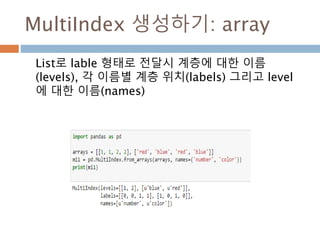
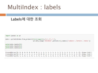
Python_numpy_pandas_matplotlib 이해하기_20160815
Download as pptx, pdf43 likes8,655 views

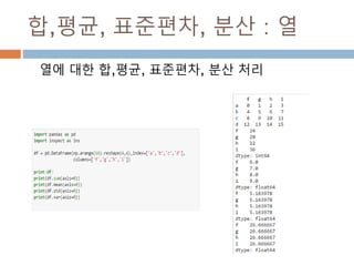
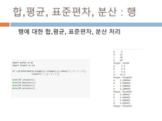
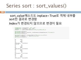
하나로 통합해서 향후 정리 예정


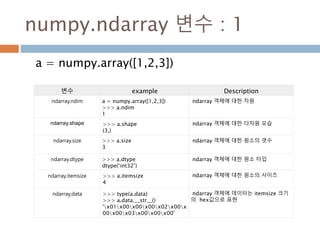

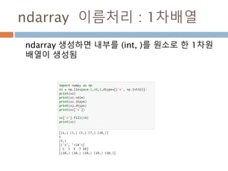
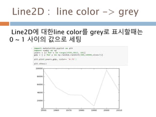
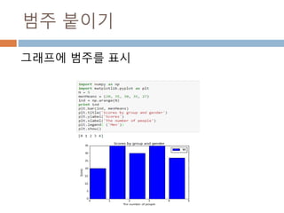
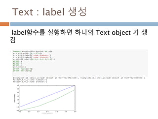
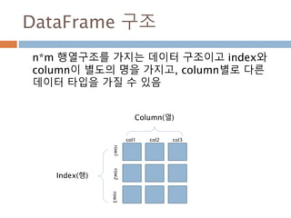
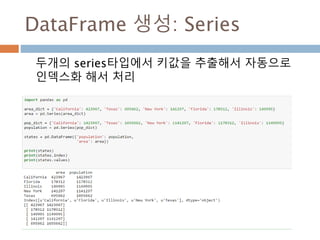
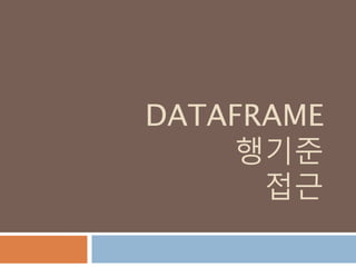
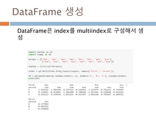
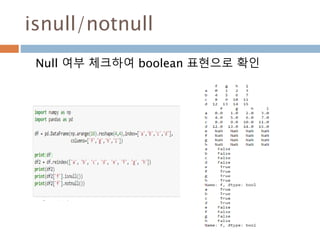
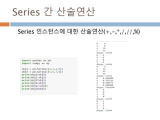
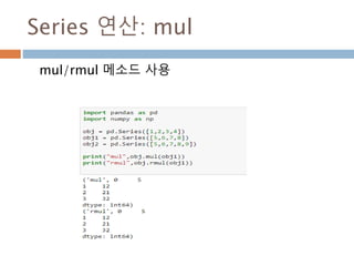
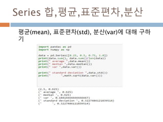
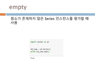
![numpy.ndarray 변수 : 1
a = numpy.array([1,2,3])
변수 example Description
ndarray.ndim a = numpy.array([1,2,3])
>>> a.ndim
1
ndarray 객체에 대한 차원
ndarray.shape >>> a.shape
(3,)
ndarray 객체에 대한 다차원 모습
ndarray.size >>> a.size
3
ndarray 객체에 대한 원소의 갯수
ndarray.dtype >>> a.dtype
dtype(‘int32’)
ndarray 객체에 대한 원소 타입
ndarray.itemsize >>> a.itemsize
4
ndarray 객체에 대한 원소의 사이즈
ndarray.data >>> type(a.data)
>>> a.data.__str__()
'x01x00x00x00x02x00x
00x00x03x00x00x00'
ndarray 객체에 데이터는 itemsize 크기
의 hex값으로 표현
13](https://image.slidesharecdn.com/pythonnumpy-160804042235/85/Python_numpy_pandas_matplotlib-_20160815-13-320.jpg)
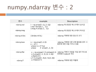
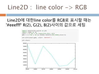
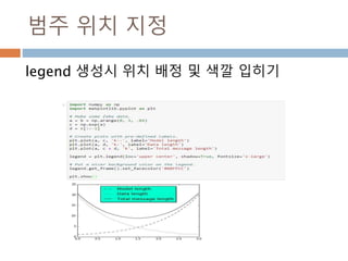
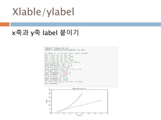
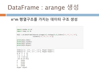
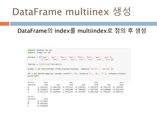
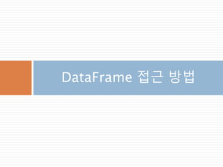
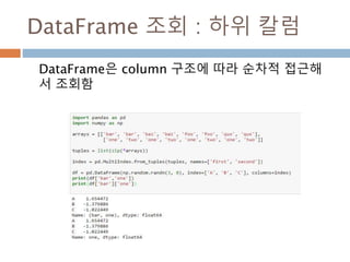
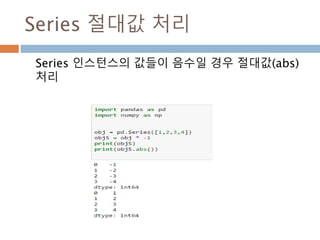
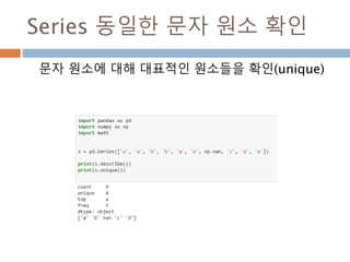
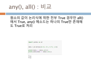
![numpy.ndarray 변수 : 2
변수 example Description
ndarray.real i = np.array([1+2j, 2+3j])
i.real #array([ 1., 2.])
i.imag # array([ 2., 3.])
ndarray 에 생성된 복소수에서 실수값
ndarray.imag ndarray 에 생성된 복소수에서 허수값
ndarray.strides i.Strides #(16,) ndarray 객체에 대한 원소의 크기
ndarray.base x = np.array([1,2,3])
y = x[1:]
y.base is x # True
y.base # array([1, 2, 3])
ndarray 객체에 다른 곳에 할당할 경우 그
원천에 대한 것을 가지고 있음
ndarray.flat x = np.arange(1,7).reshape(2,3)
x # array([[1, 2, 3], [4, 5, 6]])
x.flat[3] # 4
x.T # array([[1, 4],[2, 5],[3, 6]])
x.T.flat[3] # 5
ndarray 객체가 차원을 가질 경우 하나로
연계해서 index로 처리
ndarray.T ndarray 객체에 대한 역핼력
14](https://image.slidesharecdn.com/pythonnumpy-160804042235/85/Python_numpy_pandas_matplotlib-_20160815-14-320.jpg)


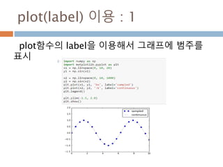
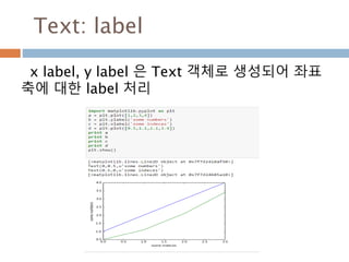
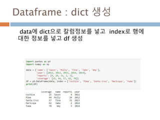
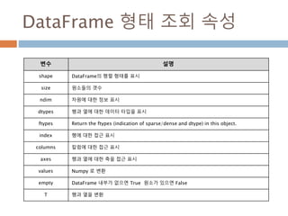
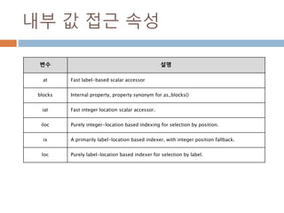
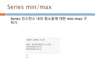
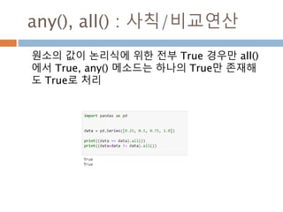
![ndarray 클래스 이해하기 1
ndarray는 각 원소별로 동일한 데이터 타입으로 처
리
원소 원소 원소array( [ ]), ,
33](https://image.slidesharecdn.com/pythonnumpy-160804042235/85/Python_numpy_pandas_matplotlib-_20160815-33-320.jpg)
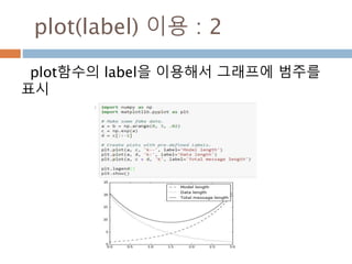
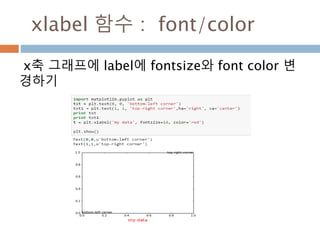
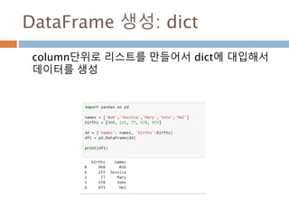
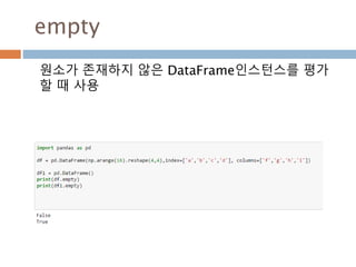
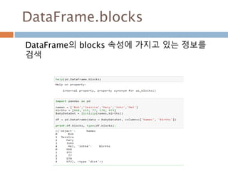
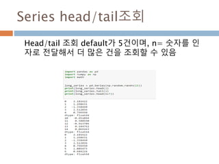
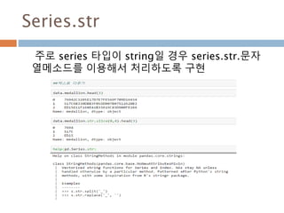
![ndarray 클래스 이해하기 2
ndarray는 각 원소내의 데이터 타입을 다양하게 구
성할 수 있음
원소 원소 원소
numpy.int_ numpy.float_ numpy.bool_
array( [ ]), ,( )
34](https://image.slidesharecdn.com/pythonnumpy-160804042235/85/Python_numpy_pandas_matplotlib-_20160815-34-320.jpg)


![배열 이해하기
3행, 3열의 배열을 기준으로 어떻게 내부를 행과 열
로 처리하는 지를 이해
[0,0] [0,1] [0,2]
[1,0] [1,1] [1,2]
[2,0] [2,1] [2,2]
Row : 행
Column: 열
0
1
2
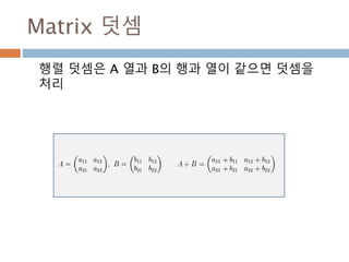
0 1 2
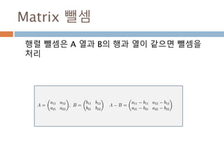
Index 접근 표기법
배열명[행][열]
배열명[행, 열]
Slice 접근 표기법
배열명[슬라이스, 슬라이스]
45](https://image.slidesharecdn.com/pythonnumpy-160804042235/85/Python_numpy_pandas_matplotlib-_20160815-45-320.jpg)


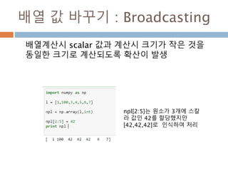

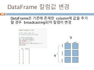
![배열 값 바꾸기 : Broadcasting
배열계산시 scalar 값과 계산시 크기가 작은 것을
동일한 크기로 계산되도록 확산이 발생
npl[2:5]는 원소가 3개에 스칼
라 값인 42를 할당했지만
[42,42,42]로 인식하여 처리
69](https://image.slidesharecdn.com/pythonnumpy-160804042235/85/Python_numpy_pandas_matplotlib-_20160815-69-320.jpg)


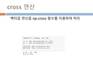

![vector 곱셈
벡터곱(vector곱, 영어: cross product) 또는 외적
(外積)은 수학에서 3차원 공간의 벡터들간의 이항연
산의 일종이다. 연산의 결과가 스칼라인 스칼라곱과
는 달리 연산의 결과가 벡터
a = [0,0,1]
b = [0,1,0]
a*b = [0-1,0-0,0-0] = [-1,0,0]
주요 산식 :
a*b = (a2b3−a3b2, a3b1−a1b3, a1b2−a2b1)
88](https://image.slidesharecdn.com/pythonnumpy-160804042235/85/Python_numpy_pandas_matplotlib-_20160815-88-320.jpg)


![axis 이해하기 : 2차원
Axis는 배열의 축을 나타내며 0은 열이고, 1은
행을 표시
92
[0,0] [0,1] [0,2]
[1,0] [1,1] [1,2]
Row : 행
Column: 열
0
1
2
0 1 2](https://image.slidesharecdn.com/pythonnumpy-160804042235/85/Python_numpy_pandas_matplotlib-_20160815-92-320.jpg)


![배열 접근하기
행과 열의 인덱스를 지정하면 실제 값에 접근해서
보여줌
배열명[ 행 범위, 열 범위]
96](https://image.slidesharecdn.com/pythonnumpy-160804042235/85/Python_numpy_pandas_matplotlib-_20160815-96-320.jpg)
![배열 접근하기 : 행과 열구분
행으로 접근, 열로 접근
[0,0] [0,1] [0,2]
[1,0] [1,1] [1,2]
[2,0] [2,1] [2,2]
Row : 행
Column: 열
0
1
2
0 1 2
[0,0] [0,1] [0,2]
[1,0] [1,1] [1,2]
[2,0] [2,1] [2,2]
Row : 행
Column: 열
0
1
2
0 1 2
첫번째 행 접근
첫번째 열 접근
97](https://image.slidesharecdn.com/pythonnumpy-160804042235/85/Python_numpy_pandas_matplotlib-_20160815-97-320.jpg)
![배열 접근하기 : 행렬로 구분
첫번째와 두번째 행과 두번째와 세번째 열로 접근
[0,0] [0,1] [0,2]
[1,0] [1,1] [1,2]
[2,0] [2,1] [2,2]
Row : 행
Column: 열
0
1
2
0 1 2
98](https://image.slidesharecdn.com/pythonnumpy-160804042235/85/Python_numpy_pandas_matplotlib-_20160815-98-320.jpg)
![배열 접근하기 : 값
행과 열의 인덱스를 지정하면 실제 값에 접근해서
보여줌
[0,0] [0,1] [0,2]
[1,0] [1,1] [1,2]
[2,0] [2,1] [2,2]
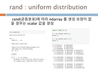
Row : 행
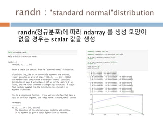
Column: 열
0
1
2
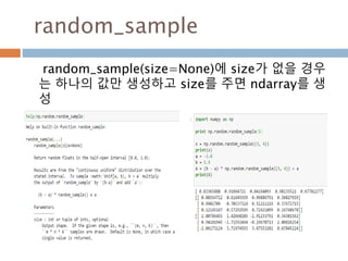
0 1 2
99](https://image.slidesharecdn.com/pythonnumpy-160804042235/85/Python_numpy_pandas_matplotlib-_20160815-99-320.jpg)
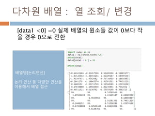
![다차원 배열 : 열 조회/ 변경
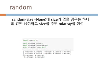
7*4배열을 정의하고 첫번째 열의 값을 99으로
변경
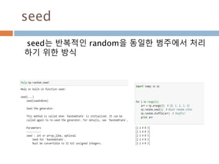
배열명[행접근, 열접근]
Slicing도 행접근과 열접근으
로 별도로 할 수 있음
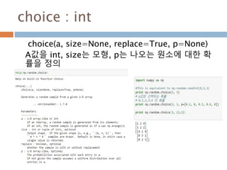
배열명[ 행 슬라이싱, 열 슬라
이싱] 으로 배열을 접근 가능
101](https://image.slidesharecdn.com/pythonnumpy-160804042235/85/Python_numpy_pandas_matplotlib-_20160815-101-320.jpg)
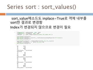
![argmax/argmin
배열 내부의 최대값과 최소값에 대한 인덱스를 검
색 가능하고 [ ] 내부에 표시하면 값을 검색
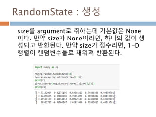
102](https://image.slidesharecdn.com/pythonnumpy-160804042235/85/Python_numpy_pandas_matplotlib-_20160815-102-320.jpg)
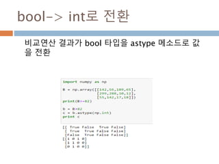

![다차원 배열 : 열 조회/ 변경
[data1 <0] =0 실제 배열의 원소들 값이 0보다 작
을 경우 0으로 전환
배열명[논리연산]
논리 연산 등 다양한 연산을
이용해서 배열 접근
105](https://image.slidesharecdn.com/pythonnumpy-160804042235/85/Python_numpy_pandas_matplotlib-_20160815-105-320.jpg)


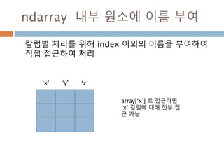


![ndarray 내부 원소에 이름 부여
칼럼별 처리를 위해 index 이외의 이름을 부여하여
직접 접근하여 처리
‘x’ ‘y’ ‘z’
array[‘x’] 로 접근하면
‘x’ 칼럼에 대해 전부 접
근 가능
117](https://image.slidesharecdn.com/pythonnumpy-160804042235/85/Python_numpy_pandas_matplotlib-_20160815-117-320.jpg)


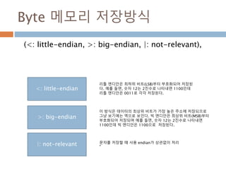


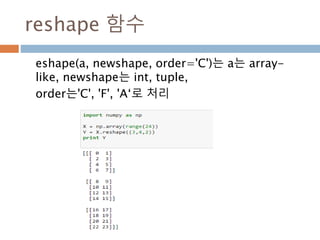
![Little-endian
숫자를 저장할때 제일 왼쪽부터 저장됨
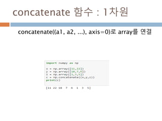
.
>>> ar = np.array([1,2,3])
>>> ar.tostring()
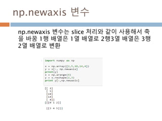
'x01x00x00x00x00x00x00x00x02x0
0x00x00x00x00x00x00x03x00x00x
00x00x00x00x00'
>>> l = ar.tosting()
>>> ar.itemsize
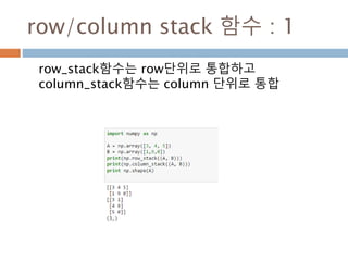
8
>>> l[0:8]
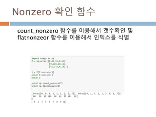
x01x00x00x00x00x00x00x00
x01x00x00x
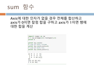
00x00x00x00
x00
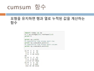
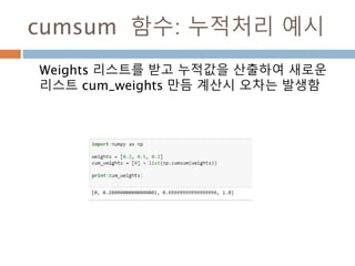
8bytes씩 저장하고
숫자는 첫번째부터
들어감
146](https://image.slidesharecdn.com/pythonnumpy-160804042235/85/Python_numpy_pandas_matplotlib-_20160815-146-320.jpg)
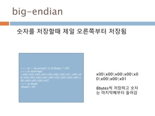
![big-endian
숫자를 저장할때 제일 오른쪽부터 저장됨
.
>>> ar = np.array([1,2,3],dtype='>i8')
>>> ar.tostring()
'x00x00x00x00x00x00x00x01x00x0
0x00x00x00x00x00x02x00x00x00x
00x00x00x00x03’
>>> ar.dtype
dtype('>i8')
x00x00x00x00x0
0x00x00x01
8bytes씩 저장하고 숫자
는 마지막째부터 들어감
147](https://image.slidesharecdn.com/pythonnumpy-160804042235/85/Python_numpy_pandas_matplotlib-_20160815-147-320.jpg)
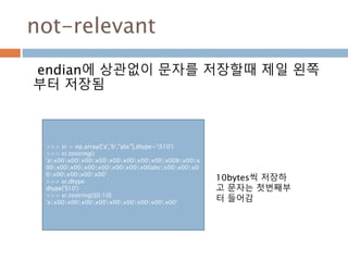
![not-relevant
endian에 상관없이 문자를 저장할때 제일 왼쪽
부터 저장됨
.
>>> sr = np.array(['a','b',"abc"],dtype='|S10')
>>> sr.tostring()
'ax00x00x00x00x00x00x00x00x00bx00x
00x00x00x00x00x00x00x00abcx00x00x0
0x00x00x00x00’
>>> sr.dtype
dtype('S10')
>>> sr.tostring()[0:10]
'ax00x00x00x00x00x00x00x00x00'
10bytes씩 저장하
고 문자는 첫번째부
터 들어감
148](https://image.slidesharecdn.com/pythonnumpy-160804042235/85/Python_numpy_pandas_matplotlib-_20160815-148-320.jpg)

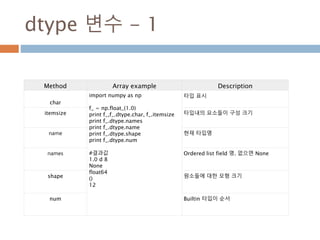
![dtype 변수 - 3
Method Array example Description
descr import numpy as np
f_ = np.float_(1.0)
print f_.dtype.descr
print f_.dtype.hasobject
print f_.dtype.subdtype
print f_.dtype.base
print f_.dtype.kind
print f_.dtype.isnative
#결과값
[('', '<f8')]
False
None
Float64
F
True
Array interface 표시
hasobject any reference-counted objects in any
fields or sub-dtypes 가 존재시 True
subdtype
Tuple (item_dtype, shape) if this dtype
describes a sub-array, and None other
wise.
base 기본 정의된 타입
kind array-protocol type
isnative 파이썬 내부 byte order 사용여부
152](https://image.slidesharecdn.com/pythonnumpy-160804042235/85/Python_numpy_pandas_matplotlib-_20160815-152-320.jpg)

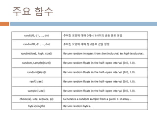
![주요 함수
rand(d0, d1, ..., dn) 주어진 모양에 대해 0에서 1사이의 균등 분포 생성
randn(d0, d1, ..., dn) 주어진 모양에 대해 정규분포 값을 생성
randint(low[, high, size]) Return random integers from low (inclusive) to high (exclusive).
random_sample([size]) Return random floats in the half-open interval [0.0, 1.0).
random([size]) Return random floats in the half-open interval [0.0, 1.0).
ranf([size]) Return random floats in the half-open interval [0.0, 1.0).
sample([size]) Return random floats in the half-open interval [0.0, 1.0).
choice(a[, size, replace, p]) Generates a random sample from a given 1-D array ..
bytes(length) Return random bytes.
156](https://image.slidesharecdn.com/pythonnumpy-160804042235/85/Python_numpy_pandas_matplotlib-_20160815-156-320.jpg)


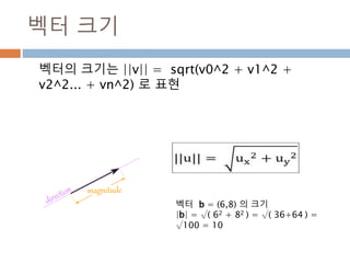
![Binomial : 이항분포
n은 trial , p는 구간 [0,1]에 성공 P는 확률
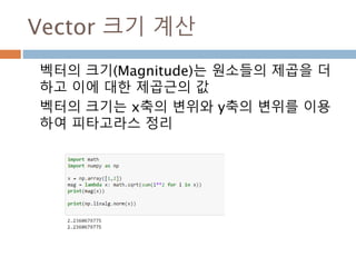
이항 분포에서 작성한 것임
180](https://image.slidesharecdn.com/pythonnumpy-160804042235/85/Python_numpy_pandas_matplotlib-_20160815-180-320.jpg)


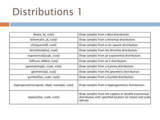
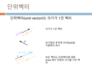
![Distributions 1
beta(a, b[, size]) Draw samples from a Beta distribution.
binomial(n, p[, size]) Draw samples from a binomial distribution.
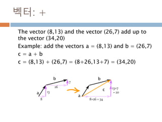
chisquare(df[, size]) Draw samples from a chi-square distribution.
dirichlet(alpha[, size]) Draw samples from the Dirichlet distribution.
exponential([scale, size]) Draw samples from an exponential distribution.
f(dfnum, dfden[, size]) Draw samples from an F distribution.
gamma(shape[, scale, size]) Draw samples from a Gamma distribution.
geometric(p[, size]) Draw samples from the geometric distribution.
gumbel([loc, scale, size]) Draw samples from a Gumbel distribution.
hypergeometric(ngood, nbad, nsample[, size]) Draw samples from a Hypergeometric distribution.
laplace([loc, scale, size])
Draw samples from the Laplace or double exponential
distribution with specified location (or mean) and scale
(decay).
183](https://image.slidesharecdn.com/pythonnumpy-160804042235/85/Python_numpy_pandas_matplotlib-_20160815-183-320.jpg)
![Distributions 2
logistic([loc, scale, size]) Draw samples from a logistic distribution.
lognormal([mean, sigma, size]) Draw samples from a log-normal distribution.
logseries(p[, size]) Draw samples from a logarithmic series distribution.
multinomial(n, pvals[, size]) Draw samples from a multinomial distribution.
multivariate_normal(mean, cov[, size])
Draw random samples from a multivariate normal distr
ibution.
negative_binomial(n, p[, size]) Draw samples from a negative binomial distribution.
noncentral_chisquare(df, nonc[, size])
Draw samples from a noncentral chi-square distributio
n.
noncentral_f(dfnum, dfden, nonc[, size]) Draw samples from the noncentral F distribution.
normal([loc, scale, size])
Draw random samples from a normal (Gaussian) distri
bution.
pareto(a[, size])
Draw samples from a Pareto II or Lomax distribution w
ith specified shape.
poisson([lam, size]) Draw samples from a Poisson distribution.
184](https://image.slidesharecdn.com/pythonnumpy-160804042235/85/Python_numpy_pandas_matplotlib-_20160815-184-320.jpg)
![Distributions 3
power(a[, size])
Draws samples in [0, 1] from a power distribution with positive ex
ponent a - 1.
rayleigh([scale, size]) Draw samples from a Rayleigh distribution.
standard_cauchy([size]) Draw samples from a standard Cauchy distribution with mode = 0.
standard_exponential([size]) Draw samples from the standard exponential distribution.
standard_gamma(shape[, size]) Draw samples from a standard Gamma distribution.
standard_normal([size])
Draw samples from a standard Normal distribution (mean=0, stde
v=1).
standard_t(df[, size])
Draw samples from a standard Student’s t distribution with df deg
rees of freedom.
triangular(left, mode, right[, size]) Draw samples from the triangular distribution.
uniform([low, high, size]) Draw samples from a uniform distribution.
vonmises(mu, kappa[, size]) Draw samples from a von Mises distribution.
wald(mean, scale[, size]) Draw samples from a Wald, or inverse Gaussian, distribution.
weibull(a[, size]) Draw samples from a Weibull distribution.
zipf(a[, size]) Draw samples from a Zipf distribution.
185](https://image.slidesharecdn.com/pythonnumpy-160804042235/85/Python_numpy_pandas_matplotlib-_20160815-185-320.jpg)


![tile
A 배열에 대한 Reps는 axis 축에 따른 반복을 표시
numpy.tile(A, reps)
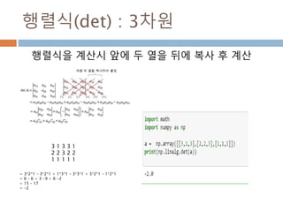
x = np.array([ [1, 2], [3, 4]])
np.tile(x, (3,4))
1. Reps가 스칼라 값은 배수만큼 증가
2. Reps가 벡터값 일 경우 행과 열에 따라 추가
200](https://image.slidesharecdn.com/pythonnumpy-160804042235/85/Python_numpy_pandas_matplotlib-_20160815-200-320.jpg)


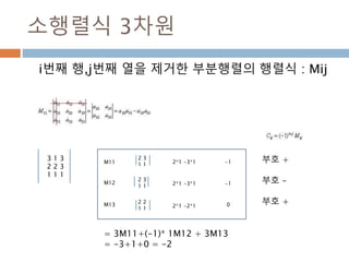


![벡터: 스칼라곱
벡터의 각 원소에 스칼라값만큼 곱하여 표시
벡터 m = [7,3]
A = 3m= [21,9]
295](https://image.slidesharecdn.com/pythonnumpy-160804042235/85/Python_numpy_pandas_matplotlib-_20160815-295-320.jpg)


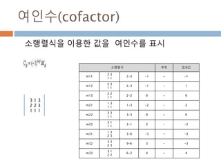
![외적 산식 : 2차원
벡터의 원소간의 cross 적을 처리
v = [a1,a2]
u = [b1,b2]
a1 a2
b1 b2
a1*b2 – a2*b1 Example: The cross product of a = (2,3) and b = (5,6)
c = a1b2 − a2b1 = 2×6− 3×5 = −3
Answer: a × b = -3
308](https://image.slidesharecdn.com/pythonnumpy-160804042235/85/Python_numpy_pandas_matplotlib-_20160815-308-320.jpg)
![외적 산식 : 3차원
벡터의 원소간의 cross 적을 처리
v = [a1,a2,a3]
u = [b1,b2,b3]
a2 a3 a1 a2
b2 b3 b1 b2
x 측 : a2*b3 – a3*b2
y 측 : a3*b1 – a1*b2
z 측 : a1*b2 – a2*b1
Example: The cross product of a = (2,3,4) and b = (5,6,7)
cx = aybz − azby = 3×7 − 4×6 = −3
cy = azbx − axbz = 4×5 − 2×7 = 6
cz = axby − aybx = 2×6 − 3×5 = −3
Answer: a × b = (−3,6,−3)
309](https://image.slidesharecdn.com/pythonnumpy-160804042235/85/Python_numpy_pandas_matplotlib-_20160815-309-320.jpg)
![inner 계산 방식
A = [[a1,b1] B = [[a2,b2]]
numpy.inner(A,B)
array([[a1*a2 + b1*b2]])
[[1*4+0*1]]
1 0 4 1
1 0
4 1
4=.
312](https://image.slidesharecdn.com/pythonnumpy-160804042235/85/Python_numpy_pandas_matplotlib-_20160815-312-320.jpg)
![outer
A = [[a1,b1]] B = [[a2,b2]]
numpy.outer(A,B)
array([[a1*a2 , a1*b2][ b1*a2, b1*b2]])
[[1*4,1*1] [0*4+0*1]]
1 0 4 1 1
0
4 1
4 1
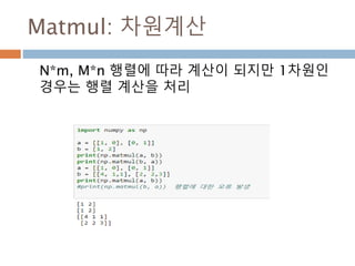
0 0
=
315](https://image.slidesharecdn.com/pythonnumpy-160804042235/85/Python_numpy_pandas_matplotlib-_20160815-315-320.jpg)


![항등행렬
모든 행렬과 닷 연산시 자기 자신이 나오게 하는
단위행렬
import numpy as np
a = np.array([[1,0],[0,1]])
b = np.array([[4,1],[3,2]])
print(np.dot(b,a))
print(np.dot(a,b))
[[4 1]
[3 2]]
[[4 1]
[3 2]]
334](https://image.slidesharecdn.com/pythonnumpy-160804042235/85/Python_numpy_pandas_matplotlib-_20160815-334-320.jpg)


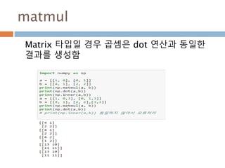


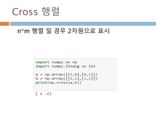
![dot : 2차원
A = [[a1,b1],[c1,d1]] B = [[a2,b2],[c2,d2]]
numpy.dot(A,B)
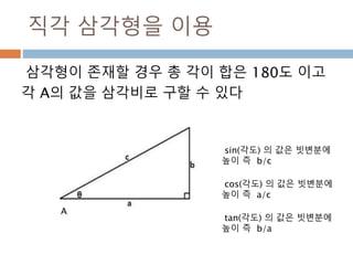
array([[a1*a2 + b1*c2, a1*b2 + b1*d2], [c1*a2 +
d1*c2, c1*b2 + d1*d2])
[[1*4+ 0*2, 1*1+0*2],[0*4+1*2, 0*1+1*2]]
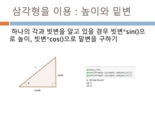
1 0
0 1
4 1
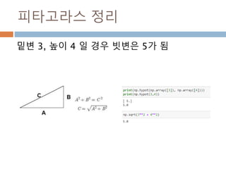
2 2
1 0
0 1
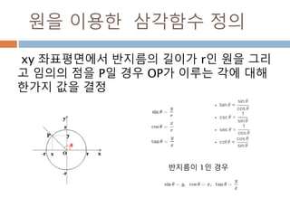
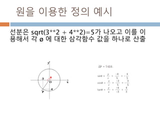
4 1
2 2
4 1
2 2
=.
347](https://image.slidesharecdn.com/pythonnumpy-160804042235/85/Python_numpy_pandas_matplotlib-_20160815-347-320.jpg)


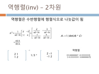
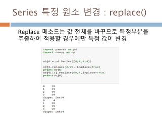
![역행렬(inv) – 2차원
역행렬은 수반행렬에 행렬식으로 나눗값이 됨
[[ 0.66666667 -0.33333333]
[-0.33333333 0.66666667]]
1/3 *
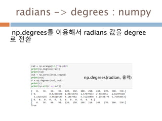
2 -1
-1 2
역행렬
2 1
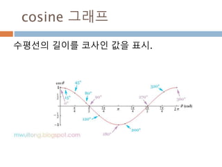
1 2
-1
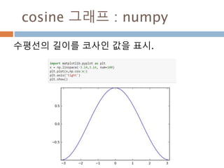
A−1=1/det(A) * CT
361](https://image.slidesharecdn.com/pythonnumpy-160804042235/85/Python_numpy_pandas_matplotlib-_20160815-361-320.jpg)
![역행렬(inv) – 3차원
역행렬은 수반행렬에 행렬식으로 나눗값이 됨
[[ 0.5 -1. 1.5]
[-0.5 0. 1.5]
[ 0. 1. -2. ]]
- 0.5 *
-1 2 -3
1 0 -3
0 -2 4
역행렬3 1 3
2 2 3
1 1 1
-1
A−1=1/det(A) * CT
362](https://image.slidesharecdn.com/pythonnumpy-160804042235/85/Python_numpy_pandas_matplotlib-_20160815-362-320.jpg)


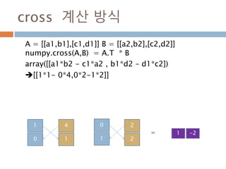
![cross 계산 방식
A = [[a1,b1],[c1,d1]] B = [[a2,b2],[c2,d2]]
numpy.cross(A,B) = A.T * B
array([[a1*b2 - c1*a2 , b1*d2 – d1*c2])
[[1*1- 0*4,0*2-1*2]]
1 0
0 1
4 2
1 2
1 -2=
369](https://image.slidesharecdn.com/pythonnumpy-160804042235/85/Python_numpy_pandas_matplotlib-_20160815-369-320.jpg)


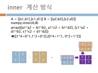
![inner 계산 방식
A = [[a1,b1],[c1,d1]] B = [[a2,b2],[c2,d2]]
numpy.inner(A,B)
array([[a1*a2 + b1*b2, a1*c2 + b1*d2], [c1*a2 +
d1*b2, c1*c2 + d1*d2])
[[1*4+0*1,1*2+0*2],[0*4+1*1, 0*2+1*2]]
1 0
0 1
4 1
2 2
1 0
0 1
4 1
2 2
4 2
1 2
=.
372](https://image.slidesharecdn.com/pythonnumpy-160804042235/85/Python_numpy_pandas_matplotlib-_20160815-372-320.jpg)
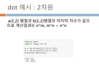
![Inner 예시 : 2차원
a(2,2) 행렬과 b(2,2)행렬의 마지막 차수가 같으
므로 계산결과는 out.shape = a.shape[:-1] +
b.shape[:-1]
373](https://image.slidesharecdn.com/pythonnumpy-160804042235/85/Python_numpy_pandas_matplotlib-_20160815-373-320.jpg)
![Inner 예시 : 3차원
a(2,3,2) 행렬과 b(2,2)행렬의 마지막 차수가 같
으므로 계산결과는 out.shape = a.shape[:-1] +
b.shape[:-1]
374](https://image.slidesharecdn.com/pythonnumpy-160804042235/85/Python_numpy_pandas_matplotlib-_20160815-374-320.jpg)

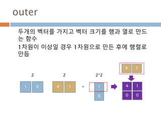
![outer: 1
Out는 두개의 벡터에 대한 행렬로 구성
out[i, j] = a[i] * b[j]
377](https://image.slidesharecdn.com/pythonnumpy-160804042235/85/Python_numpy_pandas_matplotlib-_20160815-377-320.jpg)


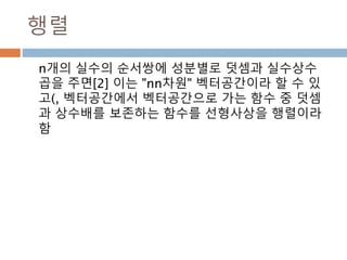
![행렬
n개의 실수의 순서쌍에 성분별로 덧셈과 실수상수
곱을 주면[2] 이는 "nn차원" 벡터공간이라 할 수 있
고(, 벡터공간에서 벡터공간으로 가는 함수 중 덧셈
과 상수배를 보존하는 함수를 선형사상을 행렬이라
함
390](https://image.slidesharecdn.com/pythonnumpy-160804042235/85/Python_numpy_pandas_matplotlib-_20160815-390-320.jpg)


![주요 함수
선형대수에 대한 함수들
함수 설명
dot(a, b[, out]) n차원 행렬 n*m m*l에 대한 production(결과는 n*l)
vdot(a, b) Vector에 대한 prodution
inner(a, b) N 차원 행렬에 대한 Inner product (행렬이 동일해야 함).
outer(a, b[, out]) 2개 벡터에 대해 계산 후 행렬로 표시.
matmul(a, b[, out]) 두 행렬에 대한 Matrix product (dot과 동일한 결과)
tensordot(a, b[, axes]) Compute tensor dot product along specified axes for arrays >= 1-D.
linalg.matrix_power(M, n) Raise a square matrix to the (integer) power n.
cross(a, b, axisa=-1, axisb=-1, axisc=-1, axis=None) 행렬에 대한 외적을 구함
einsum(subscripts, *operands[, out, dtype, ...]) Evaluates the Einstein summation convention on the operands.
kron(a, b) Kronecker product of two arrays.
408](https://image.slidesharecdn.com/pythonnumpy-160804042235/85/Python_numpy_pandas_matplotlib-_20160815-408-320.jpg)
![주요 함수
선형대수에 대한 함수들
함수 설명
linalg.cholesky(a) Cholesky decomposition.
linalg.qr(a[, mode]) Compute the qr factorization of a matrix.
linalg.svd(a[, full_matrices, compute_uv]) Singular Value Decomposition.
410](https://image.slidesharecdn.com/pythonnumpy-160804042235/85/Python_numpy_pandas_matplotlib-_20160815-410-320.jpg)

![주요 함수
선형대수에 대한 함수들
함수 설명
linalg.eig(a) Compute the eigenvalues and right eigenvectors of a square array.
linalg.eigh(a[, UPLO]) Return the eigenvalues and eigenvectors of a Hermitian or symmetric matrix.
linalg.eigvals(a) Compute the eigenvalues of a general matrix.
linalg.eigvalsh(a[, UPLO]) Compute the eigenvalues of a Hermitian or real symmetric matrix.
linalg.eig(a) Compute the eigenvalues and right eigenvectors of a square array.
412](https://image.slidesharecdn.com/pythonnumpy-160804042235/85/Python_numpy_pandas_matplotlib-_20160815-412-320.jpg)

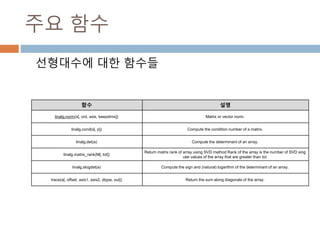
![주요 함수
선형대수에 대한 함수들
함수 설명
linalg.norm(x[, ord, axis, keepdims]) Matrix or vector norm.
linalg.cond(x[, p]) Compute the condition number of a matrix.
linalg.det(a) Compute the determinant of an array.
linalg.matrix_rank(M[, tol])
Return matrix rank of array using SVD method Rank of the array is the number of SVD sing
ular values of the array that are greater than tol.
linalg.slogdet(a) Compute the sign and (natural) logarithm of the determinant of an array.
trace(a[, offset, axis1, axis2, dtype, out]) Return the sum along diagonals of the array.
414](https://image.slidesharecdn.com/pythonnumpy-160804042235/85/Python_numpy_pandas_matplotlib-_20160815-414-320.jpg)

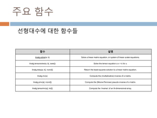
![주요 함수
선형대수에 대한 함수들
함수 설명
linalg.solve(a, b) Solve a linear matrix equation, or system of linear scalar equations.
linalg.tensorsolve(a, b[, axes]) Solve the tensor equation a x = b for x.
linalg.lstsq(a, b[, rcond]) Return the least-squares solution to a linear matrix equation.
linalg.inv(a) Compute the (multiplicative) inverse of a matrix.
linalg.pinv(a[, rcond]) Compute the (Moore-Penrose) pseudo-inverse of a matrix.
linalg.tensorinv(a[, ind]) Compute the ‘inverse’ of an N-dimensional array.
416](https://image.slidesharecdn.com/pythonnumpy-160804042235/85/Python_numpy_pandas_matplotlib-_20160815-416-320.jpg)


![등차급수
등차급수[ arithmetic series , 等差級數 ]
산술급수(算術級數)라고도 한다. 등차수열을 이
루고 있는 것을 말 함
급수 a1+a2+a3+…+an+…에서
an=an-1+d(n=2,3,…) 인 관계식
급수로 표시
546](https://image.slidesharecdn.com/pythonnumpy-160804042235/85/Python_numpy_pandas_matplotlib-_20160815-546-320.jpg)


![정적분: definite integral
리만 적분에서 다루는 고전적인 정의에 따르면 실수
의 척도를 사용하는 측도 공간에 나타낼 수 있는 연
속인 함수 f(x)에 대하여 그 함수의 정의역의 부분 집
합을 이루는 구간 [a, b] 에 대응하는 치역으로 이루
어진 곡선의 리만 합의 극한을 구하는 것이다. 이를
정적분(定積分, definite integral)이라 한다.
620](https://image.slidesharecdn.com/pythonnumpy-160804042235/85/Python_numpy_pandas_matplotlib-_20160815-620-320.jpg)


![확률밀도함수
확률밀도함수(probability density function 약
자 PDF )f(x)는 일정한 값들의 범위를 포괄하는
연속확률변수의 확률을 찾는데 사용하고 연속데
이터에서의 확률을 구하기 위해서 확률밀도함수
의 면적을 구함
703
확률 밀도함수 f(x)와 구간[a,b] 에
대해 확률변수 X가 구간에 포함될
확률 P(a<= X<=b)는](https://image.slidesharecdn.com/pythonnumpy-160804042235/85/Python_numpy_pandas_matplotlib-_20160815-703-320.jpg)

![연속균등분포
연속균등분포(continuous uniform distribution)은
연속 확률 분포로, 분포가 특정 범위 내에서 균등하
게 나타나 있을 경우를 가리킨다. 이 분포는 두 개의
매개변수 a,b를 받으며, 이때 [a,b] 범위에서 균등한
확률을 가진다.
705](https://image.slidesharecdn.com/pythonnumpy-160804042235/85/Python_numpy_pandas_matplotlib-_20160815-705-320.jpg)


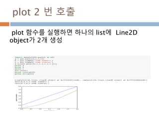
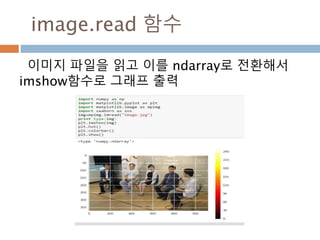
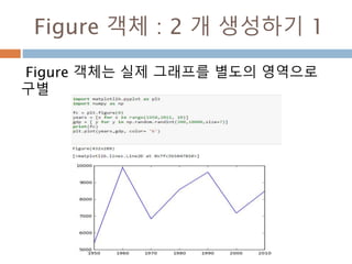
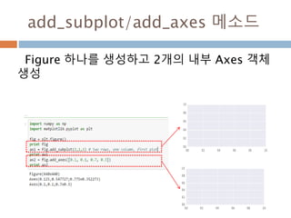
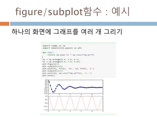
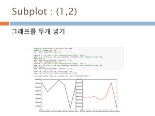
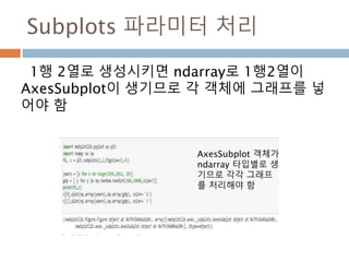
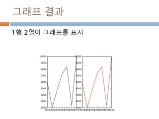
![첫번째 그래프 표시
Axes로 생성된 ax1에 plot 할당.
ax1.lines[0] 내의 저장된 것을 조회
893](https://image.slidesharecdn.com/pythonnumpy-160804042235/85/Python_numpy_pandas_matplotlib-_20160815-893-320.jpg)

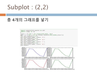
![첫번째 그래프 지우려면
del ax1.lines[0], ax1.lines.remove(line)으로
그래프 삭제
895](https://image.slidesharecdn.com/pythonnumpy-160804042235/85/Python_numpy_pandas_matplotlib-_20160815-895-320.jpg)


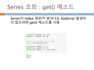


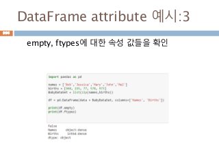


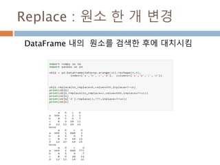
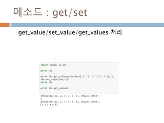
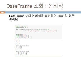
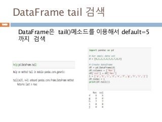
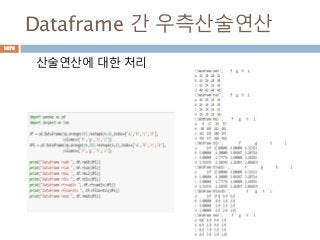
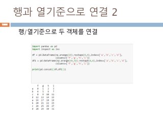
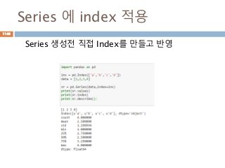
![DataFrame 행과열 검색 1
DataFrame은 ix 속성을 이용해서 행과 열을 동시
에 검색 ([ 행(슬라이싱 : ), 칼럼(명) ])
행
열
col1
row1row2row3
col2
1009](https://image.slidesharecdn.com/pythonnumpy-160804042235/85/Python_numpy_pandas_matplotlib-_20160815-1009-320.jpg)
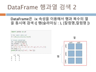
![DataFrame 행과열 검색 2
DataFrame은 ix 속성을 이용해서 행과 복수의 열
을 동시에 검색 ([ 행(슬라이싱 : ), [칼럼명,칼럼명 ])
행
열
col1
row1row2row3
col2
1010](https://image.slidesharecdn.com/pythonnumpy-160804042235/85/Python_numpy_pandas_matplotlib-_20160815-1010-320.jpg)


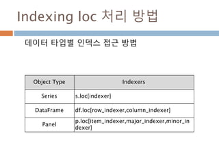
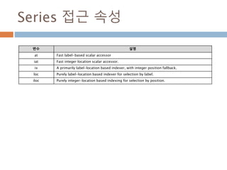
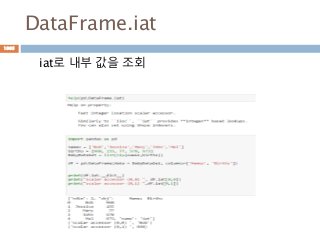
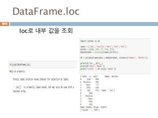
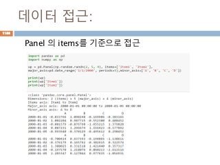
![Indexing loc 처리 방법
데이터 타입별 인덱스 접근 방법
Object Type Indexers
Series s.loc[indexer]
DataFrame df.loc[row_indexer,column_indexer]
Panel
p.loc[item_indexer,major_indexer,minor_in
dexer]
1013](https://image.slidesharecdn.com/pythonnumpy-160804042235/85/Python_numpy_pandas_matplotlib-_20160815-1013-320.jpg)

![DataFrame 단일 행 검색
DataFrame은 단일 행을 인덱스 방식([ ])
행
열
col1
row1row2row3
col2
1016](https://image.slidesharecdn.com/pythonnumpy-160804042235/85/Python_numpy_pandas_matplotlib-_20160815-1016-320.jpg)
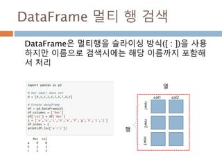
![DataFrame 멀티 행 검색
DataFrame은 멀티행을 슬라이싱 방식([ : ])을 사용
하지만 이름으로 검색시에는 해당 이름까지 포함해
서 처리
행
열
col1
row1row2row3
col2
1017](https://image.slidesharecdn.com/pythonnumpy-160804042235/85/Python_numpy_pandas_matplotlib-_20160815-1017-320.jpg)


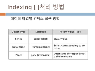
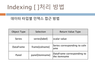
![Indexing [ ]처리 방법
데이터 타입별 인덱스 접근 방법
Object Type Selection Return Value Type
Series series[label] scalar value
DataFrame frame[colname]
Series corresponding to col
name
Panel panel[itemname]
DataFrame corresponding t
o the itemname
1021](https://image.slidesharecdn.com/pythonnumpy-160804042235/85/Python_numpy_pandas_matplotlib-_20160815-1021-320.jpg)


![DataFrame 단일 열 검색
DataFrame은 단일 열을 인덱스 방식([ ])
행
열
col1
row1row2row3
col2
1029](https://image.slidesharecdn.com/pythonnumpy-160804042235/85/Python_numpy_pandas_matplotlib-_20160815-1029-320.jpg)
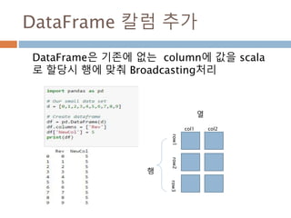
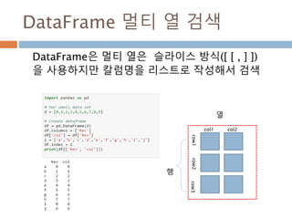
![DataFrame 멀티 열 검색
DataFrame은 멀티 열은 슬라이스 방식([ [ , ] ])
을 사용하지만 칼럼명을 리스트로 작성해서 검색
행
열
col1
row1row2row3
col2
1030](https://image.slidesharecdn.com/pythonnumpy-160804042235/85/Python_numpy_pandas_matplotlib-_20160815-1030-320.jpg)
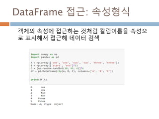
![DataFrame 접근: 사전형식
[“칼럼명”]으로 조회하면 칼럼 기준으로 접근해서
데이터 검색
1031](https://image.slidesharecdn.com/pythonnumpy-160804042235/85/Python_numpy_pandas_matplotlib-_20160815-1031-320.jpg)


![DataFrame 접근: swap처리
칼럼별 swap 처리를 하려면 indexinf[ ]처리하기
위해 리스트에 칼럼명을 사용해서 처리
1035](https://image.slidesharecdn.com/pythonnumpy-160804042235/85/Python_numpy_pandas_matplotlib-_20160815-1035-320.jpg)


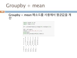
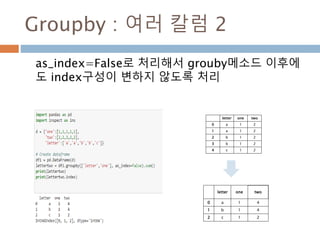
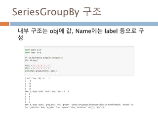
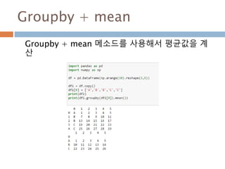
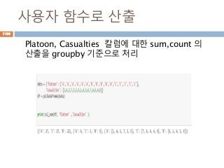
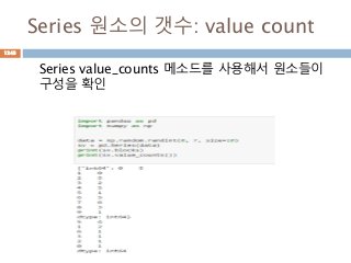
![Groupby + mean: 2개 그룹
Groupby + mean 메소드를 사용해서 2개 그룹에
대한 평균값을 계산 groupby 내의 파라미터를
칼럼구분([ , ]) 처리
1123](https://image.slidesharecdn.com/pythonnumpy-160804042235/85/Python_numpy_pandas_matplotlib-_20160815-1123-320.jpg)


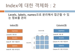
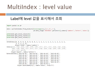
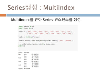
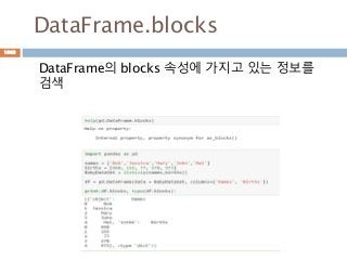
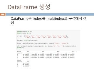
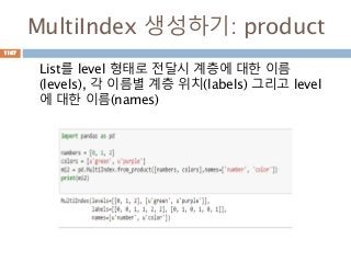
![표에 대한 메타데이터 관리
실제 데이터를 접근할 때 별도의 메타데이터로 관리
가 필요할 경우
MultiIndex(levels=[[1, 2],
[u'blue', u'red']],
labels=[[0, 0, 1, 1],
[1, 0, 1, 0]],
names=[u'number',
u'color'])
levels는 각 열의 대
표값을 list로 관리
number color
1 red
1 blue
2 red
2 blue
names는 각 열의 명
을 관리
labels는 각 열의 실
제 위치를 관리
객체화
1161](https://image.slidesharecdn.com/pythonnumpy-160804042235/85/Python_numpy_pandas_matplotlib-_20160815-1161-320.jpg)


![Indexing loc 처리 방법
데이터 타입별 인덱스 접근 방법
Object Type Indexers
Series s.loc[indexer]
DataFrame df.loc[row_indexer,column_indexer]
Panel
p.loc[item_indexer,major_indexer,minor_in
dexer]
1178](https://image.slidesharecdn.com/pythonnumpy-160804042235/85/Python_numpy_pandas_matplotlib-_20160815-1178-320.jpg)
![Indexing [ ]처리 방법
데이터 타입별 인덱스 접근 방법
Object Type Selection Return Value Type
Series series[label] scalar value
DataFrame frame[colname]
Series corresponding to coln
ame
Panel panel[itemname]
DataFrame corresponding to
the itemname
1179](https://image.slidesharecdn.com/pythonnumpy-160804042235/85/Python_numpy_pandas_matplotlib-_20160815-1179-320.jpg)


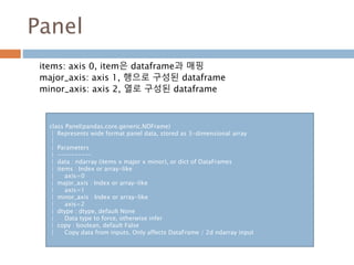
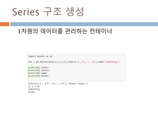
![데이터 접근 방법
Panel 클래스에서 데이터 접근법은[ ]연산자와 메소
드를 이용해서 처리
Operation Syntax Result
item wp[item] DataFrame
major_axis label wp.major_xs(val) DataFrame
minor_axis label wp.minor_xs(val) DataFrame
1187](https://image.slidesharecdn.com/pythonnumpy-160804042235/85/Python_numpy_pandas_matplotlib-_20160815-1187-320.jpg)


![Indexing loc 처리 방법
데이터 타입별 인덱스 접근 방법
Object Type Indexers
Series s.loc[indexer]
DataFrame df.loc[row_indexer,column_indexer]
Panel
p.loc[item_indexer,major_indexer,minor_in
dexer]
1194](https://image.slidesharecdn.com/pythonnumpy-160804042235/85/Python_numpy_pandas_matplotlib-_20160815-1194-320.jpg)
![Indexing [ ]처리 방법
데이터 타입별 인덱스 접근 방법
Object Type Selection Return Value Type
Series series[label] scalar value
DataFrame frame[colname]
Series corresponding to coln
ame
Panel panel[itemname]
DataFrame corresponding to
the itemname
1195](https://image.slidesharecdn.com/pythonnumpy-160804042235/85/Python_numpy_pandas_matplotlib-_20160815-1195-320.jpg)


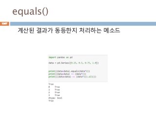


![[팝콘 시즌1] 최보경 : 실무자를 위한 인과추론 활용 - Best Practices](https://cdn.slidesharecdn.com/ss_thumbnails/papconcausalinferencebestpractices-220221141200-thumbnail.jpg?width=560&fit=bounds)


More Related Content
What's hot (20)
Similar to Python_numpy_pandas_matplotlib 이해하기_20160815 (20)


More from Yong Joon Moon (20)


Python_numpy_pandas_matplotlib 이해하기_20160815
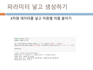
- 2. 1. NUMPY 기초 2. NUMPY 함수 3. 대수 기초 4. 선형대수 기초 5. 삼각함수 6. 지수/로그/수열 기초 목차 2
- 3. 7. 확률과 통계 기초 8.미분 기초 목차 3
- 4. 9.MATPLOTLIB 기초 10. PANDAS DATAFRAME (2차원) 11. PANDAS PANEL(3차원) 12. PANDAS SERIRES (1차원) 목차 4
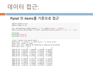
- 5. 1. NUMPY Moon Yong Joon 5
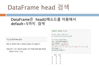
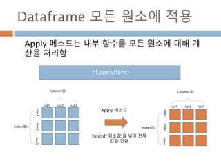
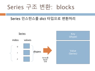
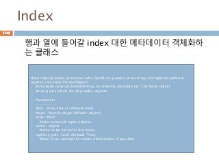
- 8. ndarray 구조 Ndarray는 데이터를 관리하고 data-type은 실제 데이터들의 값을 관리하며, array scalar는 위치를 관리 8
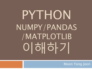
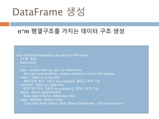
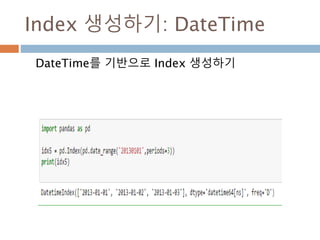
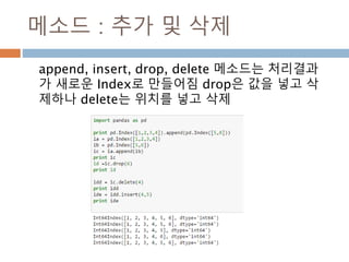
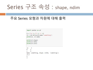
- 9. ndarray 생성 Ndarray 생성시 shape, dtype,strides이 인스턴스 속성이 생성됨 9
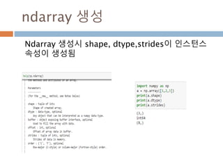
- 10. ndarray 속성 Ndarray 생성시 shape, dtype,strides이 인스턴스 속성이 생성됨 10
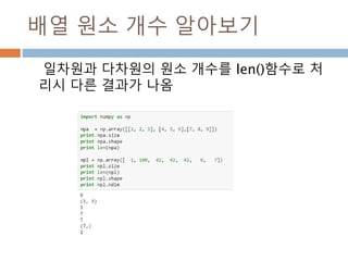
- 11. 배열 원소 개수 알아보기 일차원과 다차원의 원소 개수를 len()함수로 처 리시 다른 결과가 나옴 11
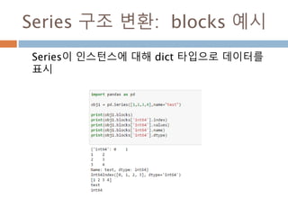
- 12. ndarray 변수12
- 13. numpy.ndarray 변수 : 1 a = numpy.array([1,2,3]) 변수 example Description ndarray.ndim a = numpy.array([1,2,3]) >>> a.ndim 1 ndarray 객체에 대한 차원 ndarray.shape >>> a.shape (3,) ndarray 객체에 대한 다차원 모습 ndarray.size >>> a.size 3 ndarray 객체에 대한 원소의 갯수 ndarray.dtype >>> a.dtype dtype(‘int32’) ndarray 객체에 대한 원소 타입 ndarray.itemsize >>> a.itemsize 4 ndarray 객체에 대한 원소의 사이즈 ndarray.data >>> type(a.data) >>> a.data.__str__() 'x01x00x00x00x02x00x 00x00x03x00x00x00' ndarray 객체에 데이터는 itemsize 크기 의 hex값으로 표현 13
- 14. numpy.ndarray 변수 : 2 변수 example Description ndarray.real i = np.array([1+2j, 2+3j]) i.real #array([ 1., 2.]) i.imag # array([ 2., 3.]) ndarray 에 생성된 복소수에서 실수값 ndarray.imag ndarray 에 생성된 복소수에서 허수값 ndarray.strides i.Strides #(16,) ndarray 객체에 대한 원소의 크기 ndarray.base x = np.array([1,2,3]) y = x[1:] y.base is x # True y.base # array([1, 2, 3]) ndarray 객체에 다른 곳에 할당할 경우 그 원천에 대한 것을 가지고 있음 ndarray.flat x = np.arange(1,7).reshape(2,3) x # array([[1, 2, 3], [4, 5, 6]]) x.flat[3] # 4 x.T # array([[1, 4],[2, 5],[3, 6]]) x.T.flat[3] # 5 ndarray 객체가 차원을 가질 경우 하나로 연계해서 index로 처리 ndarray.T ndarray 객체에 대한 역핼력 14
- 15. 할당 시 참조만 전달15
- 16. ndarray가 할당은 참조만 전달 ndarray은 참조만 할당하므로 새로운 ndarray로 처 리하려면 copy 함수나 copy 메소드를 사용해야 함 Slice을 해도 원 ndarray의 참조를 가지고 있어 갱신하면 원래 값을 변경 함 16
- 17. Range 처리 방식17
- 18. range와 numpy.arange 비교 리스트와 ndarray 타입의 차이는 배열객체 안의 메 소드들이 계산에 대한 차이가 반영 numpy.arange는 다양한 타입으로 array를 생성할 수 있음 18
- 19. 연산방식19
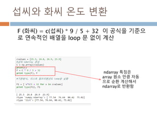
- 20. 섭씨와 화씨 온도 변환 F (화씨) = c(섭씨) * 9 / 5 + 32 이 공식을 기준으 로 연속적인 배열을 loop 문 없이 계산 ndarray 특징은 array 원소 만큼 자동 으로 순환 계산해서 ndarray로 반환함 20
- 21. 내부 원소 접근 방식21
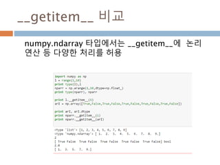
- 22. __getitem__ 비교 numpy.ndarray 타입에서는 __getitem__에 논리 연산 등 다양한 처리를 허용 22
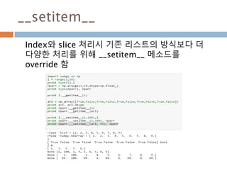
- 23. __setitem__ Index와 slice 처리시 기존 리스트의 방식보다 더 다양한 처리를 위해 __setitem__ 메소드를 override 함 23
- 24. 처리 속도24
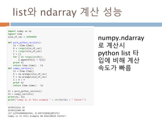
- 25. list와 ndarray 계산 성능 numpy.ndarray 로 계산시 python list 타 입에 비해 계산 속도가 빠름 25
- 26. 함수와 메소드가 이중 지원26
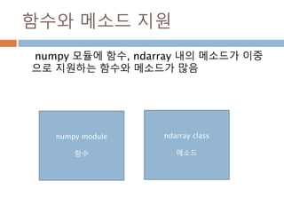
- 27. 함수와 메소드 지원 numpy 모듈에 함수, ndarray 내의 메소드가 이중 으로 지원하는 함수와 메소드가 많음 numpy module 함수 ndarray class 메소드 27
- 28. 함수와 메소드를 동일하게 처리 python은 외부 함수를 클래스 내부 변수에 할당하 면 메소드로 인식하므로 함수와 메소드를 동일하게 처리가 가능한 구조임 28
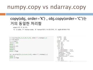
- 29. numpy.copy vs ndarray.copy copy(obj, order='K') , obj.copy(order=‘C’)는 거의 동일한 처리함 order는 {'C', 'F', 'A', 'K'}. 'C' : C-order, 'F' : Fortran-order, 'A' : fortran이면 F, 아니면 C처리, 'K' : obj에 매치해서 처리 29
- 30. 파일에 저장 및 재할당30
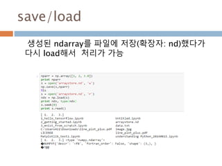
- 31. save/load 생성된 ndarray를 파일에 저장(확장자: nd)했다가 다시 load해서 처리가 가능 31
- 32. numpy 이해하기32
- 33. ndarray 클래스 이해하기 1 ndarray는 각 원소별로 동일한 데이터 타입으로 처 리 원소 원소 원소array( [ ]), , 33
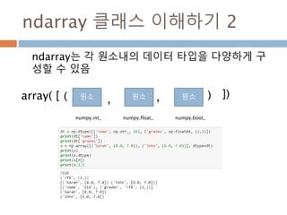
- 34. ndarray 클래스 이해하기 2 ndarray는 각 원소내의 데이터 타입을 다양하게 구 성할 수 있음 원소 원소 원소 numpy.int_ numpy.float_ numpy.bool_ array( [ ]), ,( ) 34
- 35. ndarray35
- 36. ndarray 생성하기 numpy 내의 데이터 타입은array함수와 ndarray 생성자로 생성 36
- 37. ndarray 데이터 변경 ndarray 생성하면 내부 원소들은 float 타입으로 생 성됨 37
- 38. 생성 함수 이해하기 Moon Yong Joon 38
- 39. 생성함수 : 1 Ndarray를 생성하는 함수 함수 설명 array 입력 데이터를 ndarray로 변환하며 dtype이 명시되지 않은 경우 에는 자료형을 추론해 저장 asarray 입력 데이터를 ndarray로 변환하지만 입력 데이터가 ndarray일 경우 그대로 표시 arange 내장range 함수와 유사하지만 리스트 대신 ndarray를 반환 ones 주어진 dtype과 주어진 모양을 가지는 배열을 생성하고 내용을 모 두 1로 초기화 ones_like 주어진 배열과 동일한 모양과 dtype을 가지는 배열을 새로 생성하 여 1로 초기화 zero ones와 같지만 0으로 채운다 39
- 40. 생성함수 : 2 Ndarray를 생성하는 함수 함수 설명 zeros_like ones_like와 같지만 0dmfh codnsek empty 메모리를 할당하지만 초기화가 없음 empty_like 메모리를 할당하지만 초기화가 없음 eye n*n 단위행렬 생성하고 대각선으로 1을 표시하고 나머지는 0 identity n*n 단위행렬 생성 linspace 시작과 종료 그리고 총갯수 생성을 주면 ndarray로 생성 40
- 41. array41
- 42. numpy.array 생성함수 numpy.array 함수로 생성하면 실제 ndarray 타입 이 생김 numpy.array(object, dtype=None, copy=True, order=None, subok=False, ndim=0) 42
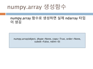
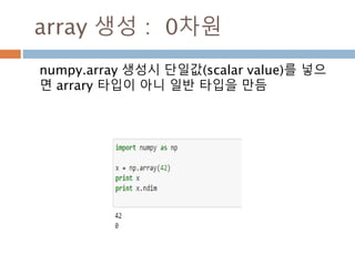
- 43. array 생성 : 0차원 numpy.array 생성시 단일값(scalar value)를 넣으 면 arrary 타입이 아니 일반 타입을 만듬 43
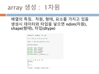
- 44. array 생성 : 1차원 배열의 특징. 차원, 형태, 요소를 가지고 있음 생성시 데이터와 타입을 넣으면 ndim(차원), shape(형태), 타입(dtype) 44
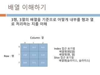
- 45. 배열 이해하기 3행, 3열의 배열을 기준으로 어떻게 내부를 행과 열 로 처리하는 지를 이해 [0,0] [0,1] [0,2] [1,0] [1,1] [1,2] [2,0] [2,1] [2,2] Row : 행 Column: 열 0 1 2 0 1 2 Index 접근 표기법 배열명[행][열] 배열명[행, 열] Slice 접근 표기법 배열명[슬라이스, 슬라이스] 45
- 46. 배열 만들기 배열의 특징. 차원, 형태, 요소를 가지고 있음 생성시 데이터와 타입을 넣으면 ndim(차원), shape(형태), 타입(dtype) 46
- 47. array 생성 :n차원 numpy.array 생성시 sequence 각 요소에 대해 접 근변수와 타임을 정할 수 있음 47
- 48. zeros48
- 49. numpy.zeros 생성자 numpy.zeros는 ndarray를 생성에 필요한 데이터 타입을 정의하기 위한 함수 numpy.zeros(shape, dtype=float, order='C') 49
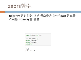
- 50. zeors함수 ndarray 생성하면 내부 원소들은 (int,float) 원소를 가지는 ndarray를 생성 50
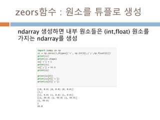
- 51. zeors함수 : 원소를 튜플로 생성 ndarray 생성하면 내부 원소들은 (int,float) 원소를 가지는 ndarray를 생성 51
- 52. numpy.zeros 생성 예시 numpy.zeros 생성시 shape를 정의하면 요소들이 값이 zero로 세팅 52
- 53. eye53
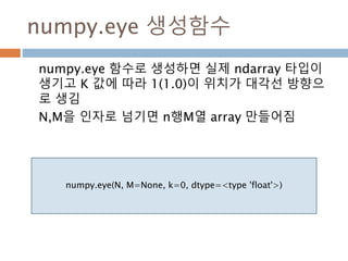
- 54. numpy.eye 생성함수 numpy.eye 함수로 생성하면 실제 ndarray 타입이 생기고 K 값에 따라 1(1.0)이 위치가 대각선 방향으 로 생김 N,M을 인자로 넘기면 n행M열 array 만들어짐 numpy.eye(N, M=None, k=0, dtype=<type 'float'>) 54
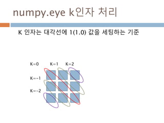
- 55. numpy.eye k인자 처리 K 인자는 대각선에 1(1.0) 값을 세팅하는 기준 K=0 K=1 K=2 K=-1 K=-2 55
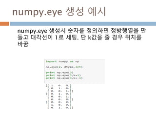
- 56. numpy.eye 생성 예시 numpy.eye 생성시 숫자를 정의하면 정방행렬을 만 들고 대각선이 1로 세팅. 단 k값을 줄 경우 위치를 바꿈 56
- 57. identity57
- 58. numpy.identity 생성함수 numpy.identiry 함수로 생성하면 실제 정방형 ndarray 타입이 생기고 대각선으로는 1이 정의됨 numpy.identity(n, dtype=None) 58
- 59. numpy.identity 생성 예시 numpy.identity 생성시 숫자를 정의하면 정방행렬 을 만들고 대각선이 1로 세팅 59
- 60. linspace60
- 61. numpy.linspace 생성함수 이 함수로 시작과 종료 그리고 num(요소의 개수)를 지점해서 생성 linspace(start, stop, num=50, endpoint=True, retstep=False) 61
- 62. linspace 주어진 값에 대해 1차원 ndarray를 만드는 random 함수 62
- 63. linspace 함수로 생성 Linspace로 특정 ndarray를 생성 63
- 64. linspace 함수로 생성 :2 Linspace로 endpoint를 false로 하면 최종 값은 포 함하지 않음 64
- 65. numpy.linspace 생성 예시 이 함수는 1차원 ndarray를 생성하고 증가된 값 단 위를 알고 싶으면 retstep 인자를 True하여 튜틀로 받아 확인하면 됨 65
- 66. arange66
- 67. arange 함수로 생성: 1 arange함수를 이용해서 생성 67
- 68. 배열 접근 및 변경하기 배열에 접근해서 값을 가져오기(index)와 배열 의 부분집합을 가져오기(slicing) 68
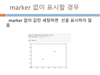
- 69. 배열 값 바꾸기 : Broadcasting 배열계산시 scalar 값과 계산시 크기가 작은 것을 동일한 크기로 계산되도록 확산이 발생 npl[2:5]는 원소가 3개에 스칼 라 값인 42를 할당했지만 [42,42,42]로 인식하여 처리 69
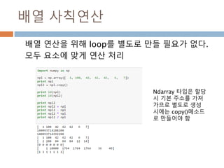
- 70. 배열 사칙연산 배열 연산을 위해 loop를 별도로 만들 필요가 없다. 모두 요소에 맞게 연산 처리 Ndarray 타입은 할당 시 기본 주소를 가져 가므로 별도로 생성 시에는 copy()메소드 로 만들어야 함 70
- 72. 연산72
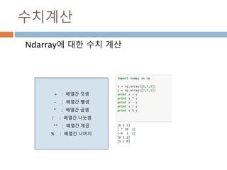
- 73. 수치계산 Ndarray에 대한 수치 계산 + : 배열간 덧셈 - : 배열간 뺄셈 * : 배열간 곱셈 / : 배열간 나눗셈 ** : 배열간 제곱 % : 배열간 나머지 73
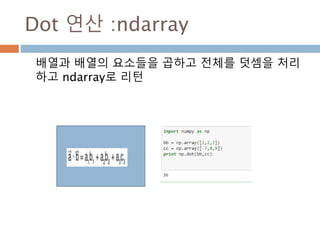
- 74. Dot 연산 :ndarray 배열과 배열의 요소들을 곱하고 전체를 덧셈을 처리 하고 ndarray로 리턴 74
- 75. Matrix 덧셈/뺄셈75
- 76. Matrix 덧셈 행렬 덧셈은 A 열과 B의 행과 열이 같으면 덧셈을 처리 76
- 77. Matrix 뺄셈 행렬 뺄셈은 A 열과 B의 행과 열이 같으면 뺄셈을 처리 77
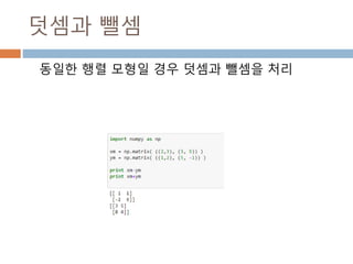
- 78. 덧셈과 뺄셈 동일한 행렬 모형일 경우 덧셈과 뺄셈을 처리 78
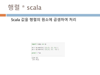
- 79. 행렬 * scala Scala 값을 행렬의 원소에 곱셈하여 처리 79
- 80. Matrix 곱셈80
- 81. Matrix 곱셈 행렬 곱셈은 A 열과 B의 행이 같으면 A 행과 B의 열 로 계산처리 됨 A(m*k) B(k*n) C(m*n) . = 81
- 82. Dot 연산 : ndarray 행렬(2행 2열)과 행렬(2행 2열)을 곱하면 결과는 2 행 2열의 행렬로 처리하고 ndarray타입으로 리턴 82
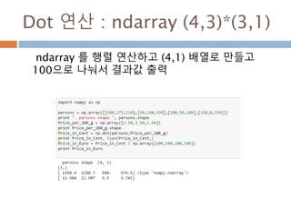
- 83. Dot 연산 : ndarray (4,3)*(3,1) ndarray 를 행렬 연산하고 (4,1) 배열로 만들고 100으로 나눠서 결과값 출력 83
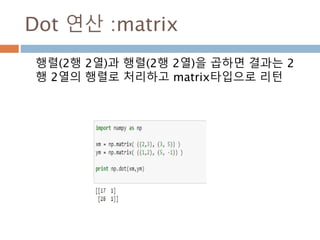
- 84. Dot 연산 :matrix 행렬(2행 2열)과 행렬(2행 2열)을 곱하면 결과는 2 행 2열의 행렬로 처리하고 matrix타입으로 리턴 84
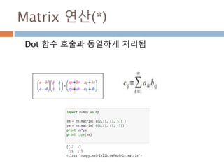
- 85. Matrix 연산(*) Dot 함수 호출과 동일하게 처리됨 85
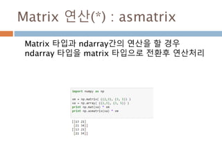
- 86. Matrix 연산(*) : asmatrix Matrix 타입과 ndarray간의 연산을 할 경우 ndarray 타입을 matrix 타입으로 전환후 연산처리 86
- 87. Vector 곱87
- 88. vector 곱셈 벡터곱(vector곱, 영어: cross product) 또는 외적 (外積)은 수학에서 3차원 공간의 벡터들간의 이항연 산의 일종이다. 연산의 결과가 스칼라인 스칼라곱과 는 달리 연산의 결과가 벡터 a = [0,0,1] b = [0,1,0] a*b = [0-1,0-0,0-0] = [-1,0,0] 주요 산식 : a*b = (a2b3−a3b2, a3b1−a1b3, a1b2−a2b1) 88
- 89. cross 연산 벡터곱 연산을 np.cross 함수를 이용하여 처리 89
- 91. 배열 축 이해91
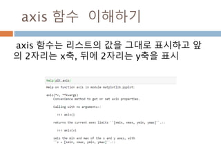
- 92. axis 이해하기 : 2차원 Axis는 배열의 축을 나타내며 0은 열이고, 1은 행을 표시 92 [0,0] [0,1] [0,2] [1,0] [1,1] [1,2] Row : 행 Column: 열 0 1 2 0 1 2
- 93. axis 이해하기 : 3차원 Axis는 배열의 축을 나타내며 두번째, 세번째의 0은 열이고, 1은 행을 표시하고 2는 첫번째와 두번째의 행을 비교 93 6 7 8 9 10 11 Row : 행 Column: 열 0 1 2 0 1 2 0 1 2 3 4 5 Row : 행 Column: 열 0 1 2 0 1 2
- 94. axis 이해하기 : 3차원 Axis는 배열의 축을 나타내며 두번째, 세번째의 0은 열이고, 1은 행을 표시하고 2는 첫번째와 두번째의 행을 비교 94 6 7 8 9 10 11 Row : 행 Column: 열 0 1 2 0 1 2 0 1 2 3 4 5 Row : 행 Column: 열 0 1 2 0 1 2
- 95. 2차원 배열 접근95
- 96. 배열 접근하기 행과 열의 인덱스를 지정하면 실제 값에 접근해서 보여줌 배열명[ 행 범위, 열 범위] 96
- 97. 배열 접근하기 : 행과 열구분 행으로 접근, 열로 접근 [0,0] [0,1] [0,2] [1,0] [1,1] [1,2] [2,0] [2,1] [2,2] Row : 행 Column: 열 0 1 2 0 1 2 [0,0] [0,1] [0,2] [1,0] [1,1] [1,2] [2,0] [2,1] [2,2] Row : 행 Column: 열 0 1 2 0 1 2 첫번째 행 접근 첫번째 열 접근 97
- 98. 배열 접근하기 : 행렬로 구분 첫번째와 두번째 행과 두번째와 세번째 열로 접근 [0,0] [0,1] [0,2] [1,0] [1,1] [1,2] [2,0] [2,1] [2,2] Row : 행 Column: 열 0 1 2 0 1 2 98
- 99. 배열 접근하기 : 값 행과 열의 인덱스를 지정하면 실제 값에 접근해서 보여줌 [0,0] [0,1] [0,2] [1,0] [1,1] [1,2] [2,0] [2,1] [2,2] Row : 행 Column: 열 0 1 2 0 1 2 99
- 100. N차원 배열 처리100
- 101. 다차원 배열 : 열 조회/ 변경 7*4배열을 정의하고 첫번째 열의 값을 99으로 변경 배열명[행접근, 열접근] Slicing도 행접근과 열접근으 로 별도로 할 수 있음 배열명[ 행 슬라이싱, 열 슬라 이싱] 으로 배열을 접근 가능 101
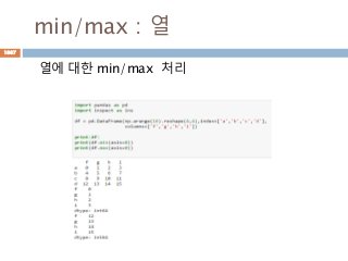
- 102. argmax/argmin 배열 내부의 최대값과 최소값에 대한 인덱스를 검 색 가능하고 [ ] 내부에 표시하면 값을 검색 102
- 103. 비교연산 처리103
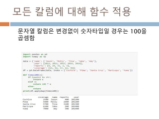
- 104. ndarray 와 비교연산 처리 ndarray와 ndarray간의 비교연산. Scala 값은 broadcasting하므로 ndarray 동일 모형의 동일값 으로 인지해서 처리된 후 bool값을 가지는 ndarray 가 생성됨 ndarray 비교연산 ndarrayndarray = 104
- 105. 다차원 배열 : 열 조회/ 변경 [data1 <0] =0 실제 배열의 원소들 값이 0보다 작 을 경우 0으로 전환 배열명[논리연산] 논리 연산 등 다양한 연산을 이용해서 배열 접근 105
- 106. 1차원 배열에 비교연산 ndarray 와 scala 값을 비교 분석하면 broadcasting하여 처리 106
- 107. 2차원 배열에 비교연산 ndarray 와 scala 값을 비교 분석하면 broadcasting하여 처리 107
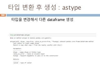
- 108. bool-> int로 전환 비교연산 결과가 bool 타입을 astype 메소드로 값 을 전환 108
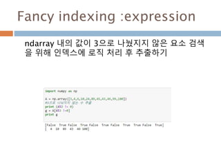
- 109. Fancy Indexing109
- 110. Fancy indexing : boolean Ndarray 내부의 요소들을 ndarray 인덱싱으로 접 근해서 추출 하는 방식 110
- 111. Fancy indexing : 숫자 1행 행축과 열축을 조합해서 처리하므로 e0는 첫번째 행만 e1은 열에 대해 처리 111
- 112. Fancy indexing : 숫자 여러 행 행축과 열축을 조합해서 처리하므로 e0는 첫번째 첫번째 행과 두번째 행만 e1은 열에 대해 처리 112
- 113. Fancy indexing :expression ndarray 내의 값이 3으로 나눴지지 않은 요소 검색 을 위해 인덱스에 로직 처리 후 추출하기 113
- 114. Fancy indexing :nonzero Nonzero 메소드를 이용해서 zero 값이 아닌 행 인 덱스와 열 인덱스를 ndarray로 전환해서 처리를 확 인해서 추출하기 114
- 116. dtype 구조116
- 117. ndarray 내부 원소에 이름 부여 칼럼별 처리를 위해 index 이외의 이름을 부여하여 직접 접근하여 처리 ‘x’ ‘y’ ‘z’ array[‘x’] 로 접근하면 ‘x’ 칼럼에 대해 전부 접 근 가능 117
- 118. Array 구조화 : string dtype 내의 타입 앞에 숫자를 지정하면 1차원적인 요소들이 생기고 튜플로 표시하면 다차원적인 표현 이 생기 118
- 119. dtype 내부 이름부여119
- 120. Array 구조화 : list 이용 dtype 내의 리스트 내에 쌍으로 이름과 타입을 정의 하고 뒤에 인자에 차원을 넣으로 차원만큼 생김 120
- 121. ndarray 이름처리 : 1차배열 ndarray 생성하면 내부를 (int, )를 원소로 한 1차원 배열이 생성됨 121
- 122. Array 구조화 : dict 이용 -1 dtype 내의 dict 내 에 names에 칼럼명 정의, formats에 타입정의 122
- 123. Array 구조화 : dict 이용 - 2 dtype 내의 dict 내 에 타입, 칼럼index, 칼럼명을 가지는 Key를 정의. Key와 칼럼명으로 접근이 가능 123
- 124. ndarray 이름처리 : 2차배열 1 ndarray 생성하면 내부를 (int, )를 원소로 한 2차원 배열이 생성됨 124
- 125. ndarray 이름처리 : 2차배열 2 ndarray 생성하면 내부를 (int, float)를 원소로 한 2차원 배열이 생성됨 125
- 126. ndarray 접근 방법126
- 127. numpy.array 접근 방법 numpy.array 생성시 sequence 각 요소에 대해 접 근변수와 타입을 정할 수 있음 해당 이름에 해 당되는 위치의 모든 값을 ndarray 타입 으로 출력 인덱스를 찾고 내부의 이름으 로 검색 127
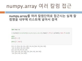
- 128. numpy.array 여러 칼럼 접근 numpy.array를 여러 칼럼단위로 접근시는 실제 칼 럼명을 내부에 리스트에 넣어서 검색 128
- 129. numpy.array 변경 방법 numpy.array 생성시 sequence 각 요소에 대해 접 근변수에 대한 값을 변경할 있음 129
- 130. ndarray 필드명 변경130
- 131. 칼럼 필드명 변경 dtype 내의 names 변수로 칼럼 필드를 조회 및 갱 신이 가능 131
- 133. 데이터 타입 이해하기133
- 134. Data type : 1 numpy 내에 정의된 데이터 타입 Data type Description bool_ Boolean (True or False) stored as a byte int_ Default integer type (same as C long; normally either int64 or int32) intc Identical to C int (normally int32 or int64) intp Integer used for indexing (same as C ssize_t; normally either int32 or int64) int8 Byte (-128 to 127) int16 Integer (-32768 to 32767) int32 Integer (-2147483648 to 2147483647) int64 Integer (-9223372036854775808 to 9223372036854775807) uint8 Unsigned integer (0 to 255) uint16 Unsigned integer (0 to 65535) uint32 Unsigned integer (0 to 4294967295) uint64 Unsigned integer (0 to 18446744073709551615) 134
- 135. Data type : 2 numpy 내에 정의된 데이터 타입 Data type Description float_ Shorthand for float64. float16 Half precision float: sign bit, 5 bits exponent, 10 bits mantissa float32 Single precision float: sign bit, 8 bits exponent, 23 bits mantissa float64 Double precision float: sign bit, 11 bits exponent, 52 bits mantissa complex_ Shorthand for complex128. complex64 Complex number, represented by two 32-bit floats (real and imaginary components) complex128 Complex number, represented by two 64-bit floats (real and imaginary components) 135
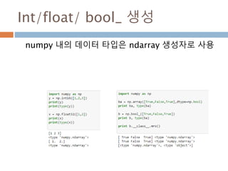
- 136. Int/float/ bool_ 생성 numpy 내의 데이터 타입은 ndarray 생성자로 사용 136
- 137. numpy.dtype137
- 138. numpy.dtype 생성자 numpy.dtype은 ndarray를 생성에 필요한 데이터 타입을 정의하기 위한 클래스 numpy.dtype(object, align=False, copy=False) 138
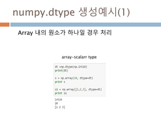
- 139. numpy.dtype 생성예시(1) Array 내의 원소가 하나일 경우 처리 array-scalar type 139
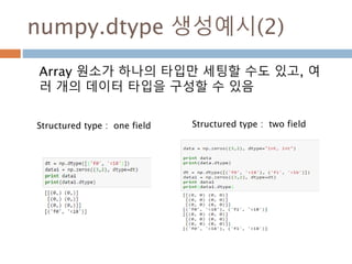
- 140. numpy.dtype 생성예시(2) Array 원소가 하나의 타입만 세팅할 수도 있고, 여 러 개의 데이터 타입을 구성할 수 있음 Structured type : two fieldStructured type : one field 140
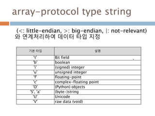
- 141. array-protocol type string (<: little-endian, >: big-endian, |: not-relevant) 와 연계처리하여 데이터 타입 지정 기본 타입 설명 ‘t’ Bit field 'b' boolean 'i' (signed) integer 'u' unsigned integer 'f' floating-point 'c' complex-floating point 'O' (Python) objects 'S', 'a' (byte-)string 'U' Unicode 'V' raw data (void) . 141
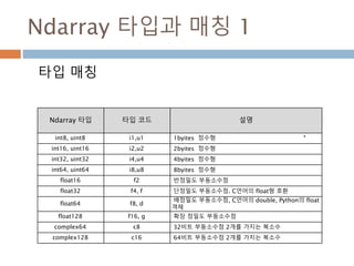
- 142. Ndarray 타입과 매칭 1 타입 매칭 Ndarray 타입 타입 코드 설명 int8, uint8 i1,u1 1byites 정수형 int16, uint16 i2,u2 2byites 정수형 int32, uint32 i4,u4 4byites 정수형 int64, uint64 i8,u8 8byites 정수형 float16 f2 반정밀도 부동소수점 float32 f4, f 단정밀도 부동소수점. C언어의 float형 호환 float64 f8, d 배정밀도 부동소수점, C언어의 double, Python의 float 객체 float128 f16, g 확장 정밀도 부동소수점 complex64 c8 32비트 부동소수점 2개를 가지는 복소수 complex128 c16 64비트 부동소수점 2개를 가지는 복소수 . 142
- 143. Ndarray 타입과 매칭2 타입 매칭 Ndarray 타입 타입 코드 설명 complex256 c32 128비트 부동소수점 2개를 가지는 복소수 bool ? True, False 값을 저장하는 불리언 형 object O 파이썬 객체형 string_ S 고정길이 문자열형-각 글자는 1바이트 unicode_ U 고정길이 유니코드 . 143
- 144. 메모리 처리 방식144
- 145. Byte 메모리 저장방식 (<: little-endian, >: big-endian, |: not-relevant), . <: little-endian >: big-endian |: not-relevant 리틀 엔디안은 최하위 비트(LSB)부터 부호화되어 저장된 다. 예를 들면, 숫자 12는 2진수로 나타내면 1100인데 리틀 엔디안은 0011로 각각 저장된다. 이 방식은 데이터의 최상위 비트가 가장 높은 주소에 저장되므로 그냥 보기에는 역으로 보인다. 빅 엔디안은 최상위 비트(MSB)부터 부호화되어 저장되며 예를 들면, 숫자 12는 2진수로 나타내면 1100인데 빅 엔디안은 1100으로 저장된다. 문자를 저장할 때 사용 endian가 상관없이 처리 145
- 146. Little-endian 숫자를 저장할때 제일 왼쪽부터 저장됨 . >>> ar = np.array([1,2,3]) >>> ar.tostring() 'x01x00x00x00x00x00x00x00x02x0 0x00x00x00x00x00x00x03x00x00x 00x00x00x00x00' >>> l = ar.tosting() >>> ar.itemsize 8 >>> l[0:8] x01x00x00x00x00x00x00x00 x01x00x00x 00x00x00x00 x00 8bytes씩 저장하고 숫자는 첫번째부터 들어감 146
- 147. big-endian 숫자를 저장할때 제일 오른쪽부터 저장됨 . >>> ar = np.array([1,2,3],dtype='>i8') >>> ar.tostring() 'x00x00x00x00x00x00x00x01x00x0 0x00x00x00x00x00x02x00x00x00x 00x00x00x00x03’ >>> ar.dtype dtype('>i8') x00x00x00x00x0 0x00x00x01 8bytes씩 저장하고 숫자 는 마지막째부터 들어감 147
- 148. not-relevant endian에 상관없이 문자를 저장할때 제일 왼쪽 부터 저장됨 . >>> sr = np.array(['a','b',"abc"],dtype='|S10') >>> sr.tostring() 'ax00x00x00x00x00x00x00x00x00bx00x 00x00x00x00x00x00x00x00abcx00x00x0 0x00x00x00x00’ >>> sr.dtype dtype('S10') >>> sr.tostring()[0:10] 'ax00x00x00x00x00x00x00x00x00' 10bytes씩 저장하 고 문자는 첫번째부 터 들어감 148
- 149. numpy.dtype 변수149
- 150. dtype 변수 - 1 Method Array example Description char import numpy as np f_ = np.float_(1.0) print f_,f_.dtype.char, f_.itemsize print f_.dtype.names print f_.dtype.name print f_.dtype.shape print f_.dtype.num #결과값 1.0 d 8 None float64 () 12 타입 표시 itemsize 타입내의 요소들이 구성 크기 name 현재 타입명 names Ordered list field 명. 없으면 None shape 원소들에 대한 모형 크기 num Builtin 타입이 순서 150
- 151. dtype 변수 - 2 Method Array example Description type import numpy as np f_ = np.float_(1.0) print f_.dtype.type print f_.dtype.str print f_.dtype.isbuiltin print f_.dtype.byteorder print f_.dtype.alignment print f_.dtype.isalignedstruct #결과값 <type 'numpy.float64'> <f8 1 = 8 False numpy 내의 타입으로 표시 str Array-protocol 타입스트링 표시 <: little-endian으로 float 8개 bytes 처리 isbuiltin 0:structure array type 1: numpy 내부 타입 2: 사용자 정의 타입 byteorder = : 기본 < : little > : big | : not applicable alignment 타입내의 요소들이 구성 크기 isalignedstruct ? 151
- 152. dtype 변수 - 3 Method Array example Description descr import numpy as np f_ = np.float_(1.0) print f_.dtype.descr print f_.dtype.hasobject print f_.dtype.subdtype print f_.dtype.base print f_.dtype.kind print f_.dtype.isnative #결과값 [('', '<f8')] False None Float64 F True Array interface 표시 hasobject any reference-counted objects in any fields or sub-dtypes 가 존재시 True subdtype Tuple (item_dtype, shape) if this dtype describes a sub-array, and None other wise. base 기본 정의된 타입 kind array-protocol type isnative 파이썬 내부 byte order 사용여부 152
- 153. dtype 변수 - 4 Method Array example Description flags import numpy as np f_ = np.float_(1.0) print f_.dtype.flags print f_.dtype.fields print f_.dtype.metadata #결과값 0 None None Interpret 되어진 bit flags fields Dtype 정의한 필드들 metadata ? 153
- 156. 주요 함수 rand(d0, d1, ..., dn) 주어진 모양에 대해 0에서 1사이의 균등 분포 생성 randn(d0, d1, ..., dn) 주어진 모양에 대해 정규분포 값을 생성 randint(low[, high, size]) Return random integers from low (inclusive) to high (exclusive). random_sample([size]) Return random floats in the half-open interval [0.0, 1.0). random([size]) Return random floats in the half-open interval [0.0, 1.0). ranf([size]) Return random floats in the half-open interval [0.0, 1.0). sample([size]) Return random floats in the half-open interval [0.0, 1.0). choice(a[, size, replace, p]) Generates a random sample from a given 1-D array .. bytes(length) Return random bytes. 156
- 157. ran/rand157
- 158. rand : uniform distribution rand(균등분포)에 따라 ndarray 를 생성 모양이 없 을 경우는 scalar 값을 생성 158
- 159. randn : "standard normal"distribution randn(정규분포)에 따라 ndarray 를 생성 모양이 없을 경우는 scalar 값을 생성 159
- 160. randint160
- 161. randint randint(low, high=None, size=None)는 최저값, 최고값-1, 총 길이 인자를 넣어 ndarray로 리턴 Size에 tuple로 선언시 다차원 생성 161
- 162. random_sample162
- 163. random_sample random_sample(size=None)에 size가 없을 경우 는 하나의 값만 생성하고 size를 주면 ndarray를 생 성 163
- 164. ranf164
- 165. ranf ranf(size=None)에 size가 없을 경우는 하나의 값 만 생성하고 size를 주면 ndarray를 생성 165
- 166. random166
- 167. random random(size=None)에 size가 없을 경우는 하나 의 값만 생성하고 size를 주면 ndarray를 생성 167
- 168. seed168
- 169. seed seed는 반복적인 random을 동일한 범주에서 처리 하기 위한 방식 169
- 170. choice170
- 171. choice : int choice(a, size=None, replace=True, p=None) A값을 int, size는 모형, p는 나오는 원소에 대한 확 률을 정의 171
- 172. choice : replace 속성 choice(a, size=None, replace=True, p=None) a값을 array, size는 모형,replace=False는 사이즈 변경 불가, p는 나오는 원소에 대한 확률을 정의 172
- 173. Permutations(순열)173
- 174. Permutation 선택된 배열의 원소를 섞기 174
- 175. shuffle 선택된 배열의 원소를 섞기 175
- 176. Random generator176
- 177. RandomState : 생성 size를 argument로 취하는데 기본값은 None 이다. 만약 size가 None이라면, 하나의 값이 생 성되고 반환된다. 만약 size가 정수라면, 1-D 행렬이 랜덤변수들로 채워져 반환된다. 177
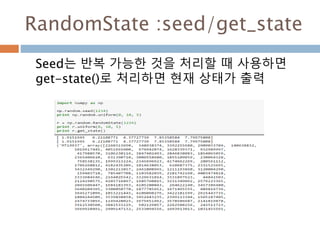
- 178. RandomState :seed/get_state Seed는 반복 가능한 것을 처리할 때 사용하면 get-state()로 처리하면 현재 상태가 출력 178
- 179. Distributions179
- 180. Binomial : 이항분포 n은 trial , p는 구간 [0,1]에 성공 P는 확률 이항 분포에서 작성한 것임 180
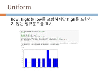
- 181. Uniform [low, high)는 low를 포함하지만 high를 포함하 지 않는 정규분로를 표시 181
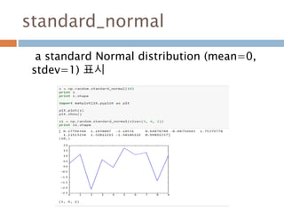
- 182. standard_normal a standard Normal distribution (mean=0, stdev=1) 표시 182
- 183. Distributions 1 beta(a, b[, size]) Draw samples from a Beta distribution. binomial(n, p[, size]) Draw samples from a binomial distribution. chisquare(df[, size]) Draw samples from a chi-square distribution. dirichlet(alpha[, size]) Draw samples from the Dirichlet distribution. exponential([scale, size]) Draw samples from an exponential distribution. f(dfnum, dfden[, size]) Draw samples from an F distribution. gamma(shape[, scale, size]) Draw samples from a Gamma distribution. geometric(p[, size]) Draw samples from the geometric distribution. gumbel([loc, scale, size]) Draw samples from a Gumbel distribution. hypergeometric(ngood, nbad, nsample[, size]) Draw samples from a Hypergeometric distribution. laplace([loc, scale, size]) Draw samples from the Laplace or double exponential distribution with specified location (or mean) and scale (decay). 183
- 184. Distributions 2 logistic([loc, scale, size]) Draw samples from a logistic distribution. lognormal([mean, sigma, size]) Draw samples from a log-normal distribution. logseries(p[, size]) Draw samples from a logarithmic series distribution. multinomial(n, pvals[, size]) Draw samples from a multinomial distribution. multivariate_normal(mean, cov[, size]) Draw random samples from a multivariate normal distr ibution. negative_binomial(n, p[, size]) Draw samples from a negative binomial distribution. noncentral_chisquare(df, nonc[, size]) Draw samples from a noncentral chi-square distributio n. noncentral_f(dfnum, dfden, nonc[, size]) Draw samples from the noncentral F distribution. normal([loc, scale, size]) Draw random samples from a normal (Gaussian) distri bution. pareto(a[, size]) Draw samples from a Pareto II or Lomax distribution w ith specified shape. poisson([lam, size]) Draw samples from a Poisson distribution. 184
- 185. Distributions 3 power(a[, size]) Draws samples in [0, 1] from a power distribution with positive ex ponent a - 1. rayleigh([scale, size]) Draw samples from a Rayleigh distribution. standard_cauchy([size]) Draw samples from a standard Cauchy distribution with mode = 0. standard_exponential([size]) Draw samples from the standard exponential distribution. standard_gamma(shape[, size]) Draw samples from a standard Gamma distribution. standard_normal([size]) Draw samples from a standard Normal distribution (mean=0, stde v=1). standard_t(df[, size]) Draw samples from a standard Student’s t distribution with df deg rees of freedom. triangular(left, mode, right[, size]) Draw samples from the triangular distribution. uniform([low, high, size]) Draw samples from a uniform distribution. vonmises(mu, kappa[, size]) Draw samples from a von Mises distribution. wald(mean, scale[, size]) Draw samples from a Wald, or inverse Gaussian, distribution. weibull(a[, size]) Draw samples from a Weibull distribution. zipf(a[, size]) Draw samples from a Zipf distribution. 185
- 186. 2. NUMPY 함수 Moon Yong Joon 186
- 187. hypot187
- 188. hypot 함수 sqrt 함수를 ndarray 모듈도 처리할 수 있는 함 수 188
- 189. fatten/ravel189
- 190. Flatten 함수 ndarray에 대한 shape를 1차 ndarray로 전환 ‘F’: fortran 타입은 칼럼 순으 로 flat 처리함 190
- 191. ravel 함수 ndarray에 대한 shape를 1차 ndarray로 전환 ‘F’: fortran 타입은 칼럼 순으 로 flat 처리함 ‘K’: 메모리에 있는 그대로 처리 191
- 192. reshape192
- 193. reshape 함수 eshape(a, newshape, order='C')는 a는 array- like, newshape는 int, tuple, order는'C', 'F', 'A‘로 처리 193
- 194. concatenate194
- 195. concatenate 함수 : 1차원 concatenate((a1, a2, ...), axis=0)로 array를 연결 195
- 196. concatenate 함수 : n차원 concatenate((a1, a2, ...), axis=0)로 array를 연결 196
- 197. newaxis197
- 198. np.newaxis 변수 np.newaxis 변수는 slice 처리와 같이 사용해서 축 을 바꿈 1행 배열은 1열 배열로 2행3열 배열은 3행 2열 배열로 변환 198
- 199. tile199
- 200. tile A 배열에 대한 Reps는 axis 축에 따른 반복을 표시 numpy.tile(A, reps) x = np.array([ [1, 2], [3, 4]]) np.tile(x, (3,4)) 1. Reps가 스칼라 값은 배수만큼 증가 2. Reps가 벡터값 일 경우 행과 열에 따라 추가 200
- 201. Tile 함수를 이용해서 array_like를 모형에 따라 ndarray로 변환 Array_like를 ndarray로 변환 201
- 202. stack202
- 203. row_stack함수는 row단위로 통합하고 column_stack함수는 column 단위로 통합 row/column stack 함수 : 1 203
- 204. Column_stack은 행은 그대로이고 열이 추가 Row_stack은 열은 그대로이고 행의 추가 row/column stack 함수 : 2 204
- 205. count_nonzero205
- 206. Nonzero 확인 함수 count_nonzero 함수를 이용해서 갯수확인 및 flatnonzeor 함수를 이용해서 인덱스를 식별 206
- 207. sum207
- 208. sum 함수 Axis에 대한 인자가 없을 경우 전체를 합산하고 axis가 0이면 칼럼 합을 구하고 axis가 1이면 행에 대한 합을 계산 208
- 209. cumsum209
- 210. cumsum 함수 모형을 유지하면 행과 열로 누적된 값을 계산하는 함수 210
- 211. cumsum 함수: 누적처리 예시 Weights 리스트를 받고 누적값을 산출하여 새로운 리스트 cum_weights 만듬 계산시 오차는 발생함 211
- 213. 수 Moon Yong Joon 213
- 214. 수214
- 215. 수 자연수, 정수, 유리수, 무리수, 실수로 확장되는 수의 관계 215
- 216. 항등원,역수216
- 217. 항등원 항등원(恒等元)은 집합의 어떤 원소와 연산을 취 해도, 자기 자신이 되는 원소를 말한다. 쉽게 말해 서, 1개의 양을 전혀 달라 보이는 다른 양과 같게 만드는 수학적 관계를 말한다고 생각하면 된다. 217
- 218. 역수 어떤 수의 역수(逆數, 영어: reciprocal) 또는 곱 셈 역원(-逆元, 영어: multiplicative inverse)은 그 수와 곱해서 1, 즉 곱셈 항등원이 되는 수를 말 한다. x의 역수는 1/x 또는 x -1로 표기한다. 곱해서 1이 되는 두 수를 서로 역수 218
- 219. 절대값219
- 220. 절댓값은 거리의 개념이므로 반드시 0또는 양수이어야하며, 만약 실수 a가 음수라면, a에 (-1)을 곱해 양수화 절대값 absolute value 어떤 실수 a를 수직선에 대응시켰을 때, 수직선의 원점에서 실수 a까지의 거리를 의미한다. 이것을 기호로 |a|로 표시. 220
- 221. 비율221
- 222. 비율 비(比, ratio)는 어떤 수가 다른 한 수의 몇 배인지 를 나타내는 관계이다. 이 배수를 비율(比率, ratio)이라고 한다. 원주율 원의 지름에 대한 원주의 비율. 백분율 수를 100과의 비로 나타내는 것. 222
- 223. 거듭제곱223
- 224. 거듭제곱 거듭제곱은 이항 연산으로, 하나의 수를 여러 번 곱하는 연산을 의미한다. 기호로는 an 으로 표기 하며, 이때 a를 밑, n을 지수라고 한다. 224
- 225. 거듭제곱의 지수 표현 거듭제곱은 지수가 음수이면 기존 거듭제곱이 역 수가 되가 분수인 경우는 제곱근 표현이 됨 지수가 음수인 경우 지수가 분수인 경우 225
- 226. 거듭제곱의 성질 거듭제곱은 반복적인 곱하기와 나누기 처리를 하 므로 아래의 성질을 준수 226
- 227. 제곱근227
- 228. 제곱근 x의 제곱근(제곱根)은 제곱하여 x가 되는 실수를 가리키며, 특히 이 가운데 양의 제곱근을 sqrt(x) 라고 표기하고 "제곱근 x"(루트 x)라고 읽는다. 228
- 229. 제곱근의 지수 표현 제곱근 x를 수치적인 표현으로는 지수 표현을 분 수식으로 나타내면 됨 x1/2로 표현 229
- 230. 일반적으로 실수 x에 대하여 값이 부호는 +/-를 가짐 제곱근의 부호 표현 제곱근의 부호 230
- 231. 제곱근 x에 대한 수의 성질 제곱근의 값 표현 제곱근의 표현 제곱근의 값 자연수 x에 대해 결과값 은 자연수이거나 무리수이 다 음이 아닌 실수 x가 제곱 근 내부의 제곱은 x가 됨 231
- 232. 제곱근 두수 x,y에 대한 곱셈과 나눗셈 처리 방식 제곱근의 성질 제곱근의 곱셈 제곱근의 나눗셈 232
- 233. 대수의 법칙 Moon Yong Joon 233
- 234. 교환법칙234
- 235. 수학에서, 집합 S 에 이항연산 * 이 정의되어 있을 때, S의 임의의 두 원소 a, b 에 대해 a * b = b * a가 성립하면, 이 연산은 교환법칙(交換法則, commutative law)을 만족한다고 한다 교환법칙을 만족하는 연산의 예를 들어보면 다음과 같다. 유리수, 실수, 복소수에서 덧셈과 곱셈. 행렬, 벡터의 덧셈 집합의 교집합, 합집합 연산 교환법칙 수학에서 순서와 상관없이 다른 항을 바꿔 계산 해도 동일한 값이 나오는 법칙 235
- 236. 교환법칙 : 덧셈과 곱셈 수학에서 순서와 상관없이 다른 항을 바꿔 계산 해도 동일한 값이 나오는 법칙 236
- 237. 결합법칙237
- 238. 수학에서 결합법칙(結合 法則, associated law)은 한 식에서 연산 이 두 번 이상 연속될 때, 앞쪽의 연산을 먼저 계산한 값과 뒤쪽의 연산을 먼저 계산한 결과가 항상 같을 경우 그 연산은 결합법칙을 만족한다고 한다. 결합법칙을 만족하는 연산의 예를 들어보면 다음과 같다. 실수와 복소수, 사원수의 덧셈과 곱셈은 결합법칙이 성립한 다. 최대공약수와 최소공배수 함수는 결합법칙을 만족한다. 행렬 곱셈은 결합법칙을 만족한다. 결합법칙 연산이 두 번 이상 연속될 때 연산을 묶어서 처리 238
- 239. 결합법칙 연산이 두 번 이상 연속될 때 연산을 묶어서 처리 239
- 240. 분배법칙240
- 241. 집합 S와 S에 대해 닫혀있는 이항 연산 *가 정의되어 있을 때, S의 임의의 원소 a, b, c에 대해 a * (b + c) = (a * b) + (a * c)가 성립 하면 좌분배법칙이, (b + c) * a = (b * a) + (c * a)가 성립하면 우 분배법칙이 성립한다고 하며 양쪽모두 성립할 경우 집합 S에서 연 산 *에 대해 분배법칙이 성립한다고 한다. 분배법칙을 만족하는 연산의 예를 들어보면 다음과 같다. 임의의 자연수, 정수, 유리수, 실수, 복소수의 곱셈 ×은 덧 셈 +에 대해 분배법칙이 성립한다. 합집합 연산 ∪은 교집합 연산 ∩에 대해 분배법칙이 성립하 고, 교집합 연산 ∩은 합집합 연산 ∪에 대해 분배법칙이 성 립한다. 또한, 교집합 연산은 대칭자 연산에 대해 분배법칙 이 성립한다. 분배법칙 수학에서 이항연산 *와 묶음이 있을 경우 분배하 면 동일한 처리값이 나오는 법칙 241
- 242. 분배법칙 수학에서 순서와 상관없이 다른 항을 바꿔 계산 해도 동일한 값이 나오는 법칙 242
- 243. 서로소243
- 244. 공약수/최대공약수 공약수, 최대공약수, 서로소 용어 정의 공약수 두 개 또는 그 이상의 자연수가 있을 때 그 자연수들의 공통인 약수. 최대공약수 공약수들 중에서 가장 큰 수.12의 약수={1,2,3,6,12} 16의 약수={1,2,4,8,16} 18의 약수={1,2,3,6,9,18} 에서 12와 16의 공약수 → 1,2,4 → 최대공약수는 4 12, 16, 18의 공약수 → 1,2 → 최대공약수는 2 서로소 공약수가 1 하나 뿐인 두 자연수 사이의 관계 (예) 8의 약수={1,2,4,8}, 9의 약수={1,3,9}에서 8과 9의 공약수는 1 한 개 뿐이므로 8과 9는 서로소 244
- 245. 서로소 최대공약수가 1인, 둘 이상의 양의 정수들은 서로 소(relatively prime)이라고 불린다. 두 정수가 1 이외에 양의 공약수를 가지지 않으면 서로소이다. 245
- 247. 곱셈공식247
- 248. 곱셈 공식(-公式, multiplication) 다항식의 곱셈을 할 때 빠르고 편리하게 계산할 수 있도록 한 공식이다. 곱셈 공식의 양변을 바꾸 면 인수분해 공식이 된다. 248
- 249. 피타고라스 정리 피타고라스 정리를 이용해서 하나의 변수를 제곱 근 곱셈공식으로 전환해서 처리. 249
- 250. 제곱근 연산 제곱근 연산도 곱셈 공식을 이용해서 결과를 처 리 250
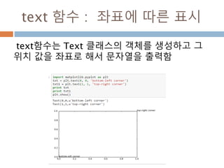
- 251. 인수분해251
- 252. 인수분해 인수 분해(因數分解, factorization)는 곱이 정의 된 집합내의 어떤 원소를 다른 원소들의 곱으로 표현하는 것을 가리킨다 252
- 253. 인수분해 공식 인수 분해 주요 공식 253
- 254. 인수분해 예시 인수 분해 주요 공식을 이용한 처리 예시 254
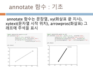
- 255. 이항정리255
- 256. 이항정리 이항정리(二項定理, binomial theorem)는 이항 다항식 x+y의 거듭제곱 (x+y)n에 대해서, 전개 한 각 항 xkyn-k의 계수 값을 구하는 정리 256
- 257. 이항정리 : 전개 다항식 (a+b)3의 전개식에서 각 항의 계수를 조 합의 수를 이용하여 나타내는 방법 (a+b)3=(a+b)(a+b)(a+b) =aaa+aab+aba+abb+baa+bab+bba+bbb =a3+3a2b+3ab2+b3 =a3+3C1a2b+3C2ab2+b3 3C1 = 3P1/1! = 3!/2!/1! = 3 3C2 = 3P2/2! = 3!/1!/2! = 3 257
- 258. 이항정리 : 파스칼 방식 다항식 (a+b)3의 전개식에서 각 항의 계수를 조 합의 수를 이용하여 나타내는 방법 258
- 260. 함수260
- 261. 함수란? 함수(函數, function) f:X→Y란 집합X와 집합 Y의 원소 사이에 주어진 다음 성질을 만족하는 대응 으로 정의된다. 261
- 262. 단사 함수란? 단사(injective) 또는 일대일(one-to-one)이라 하고 일대일인 함수를 단사함수(injection) 또는 일대일 함수(one-to-one function)이라 한다 262
- 263. 전사 함수란? 공역의 모든 원소에게 정의역의 적어도 하나의 원소 를 대응시킨다면(즉, 치역이 공역과 같다면) 전사 (surjective) 또는 X에서 Y 로(onto)의 함수라 한다. 전사인 함수를 전사함수(surjection)이라 한다. 263
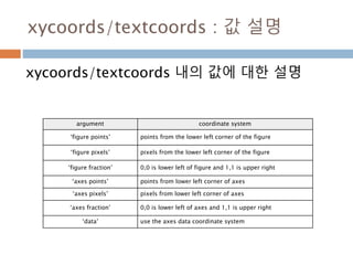
- 264. 전단사 함수란? f:X→Y가 전사이고 단사일 때 f를 전단사(bijective) 라 한다. 전단사인 함수를 전단사함수(bijection) 또 는 일대일 대응(one-to-one correspondence)라 한 다. one-to-one & onto라고도 많이 사용한다. 264
- 265. 역함수265
- 266. 역함수 f:X→Y 함수에 대한 대응관계가 반대로 되는 것을 역함수 즉 f -1: Y → X. 266
- 267. 항등함수 항등함수와 함수를 합성하면 결과는 함수와 같다. 함수와 역함수를 합성하면 항등함수가 나옴 267 =
- 268. 함수의 합성268
- 269. 함수합성 function composition 함수의 합성(函數의合成, function composition)은 한 함수의 공역이 다른 함수의 정의역과 일치하는 경 우 두 함수를 이어 하나의 함수로 만드는 연산이다. 이렇게 얻어진 함수를 합성 함수(合成函數 composite function)라고 한다. 269
- 270. 교환법칙 함수의 교환법칙은 반드시 성립하지 않는다. 270
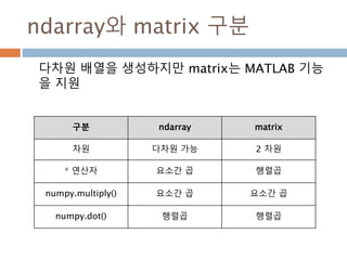
- 275. ndarray와 matrix 구분 다차원 배열을 생성하지만 matrix는 MATLAB 기능 을 지원 구분 ndarray matrix 차원 다차원 가능 2 차원 * 연산자 요소간 곱 행렬곱 numpy.multiply() 요소간 곱 요소간 곱 numpy.dot() 행렬곱 행렬곱 275
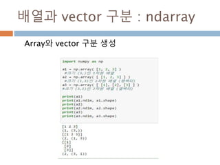
- 276. 배열과 vector 구분 : ndarray Array와 vector 구분 생성 276
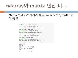
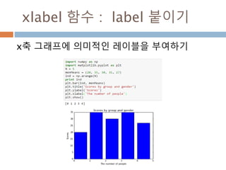
- 277. ndarray와 matrix 연산 비교 Matrix는 dot/* 처리가 동일, ndarry는 */multiply 가 동일 277
- 279. 벡터란279
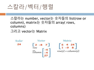
- 280. 스칼라/벡터/행렬 스칼라는 number, vector는 숫자들의 list(row or column), matrix는 숫자들의 array( rows, columns) 그리고 vector는 Matrix 280
- 281. 배열과 vertor 구분 ndarray 는 벡터 1xN, Nx1, 그리고 N크기의 1차원 배열이 모두 각각 다르며, 벡터는 그 자체로 특정 좌 표를 나타내기도 하지만 방향을 나타냄 scalar 배열 vector 양, 정적 위치 양, 정적 위치 변위, 속도, 힘(방향성) 1차원 N 차원 N 차원 단순 값 행,열 구분 없음 행벡터, 열벡터 281
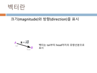
- 283. 벡터란 크기(magnitude)와 방향(direction)을 표시 벡터는 tail부터 head까지의 유향선분으로 표시 283
- 284. 벡터 크기284
- 285. 벡터 크기 벡터의 크기는 ||v|| = sqrt(v0^2 + v1^2 + v2^2... + vn^2) 로 표현 벡터 b = (6,8) 의 크기 |b| = √( 62 + 82 ) = √( 36+64 ) = √100 = 10 285
- 286. Vector 크기 계산 벡터의 크기(Magnitude)는 원소들의 제곱을 더 하고 이에 대한 제곱근의 값 벡터의 크기는 x축의 변위와 y축의 변위를 이용 하여 피타고라스 정리 286
- 287. 단위벡터287
- 288. 단위벡터 단위벡터(unit vector)는 크기가 1인 벡터 크기가 1인 벡터 표기법은 문자에 모자(hat)을 사용해서 표시 모든 벡터는 단위벡터에 대해 sclae 배수 만큼의 크기를 가진 벡 터 288
- 289. 단위벡터 정규화 해당 벡터를 0 ~ 1의 값으로 정규화 289
- 290. 산술연산290
- 291. 벡터: + The vector (8,13) and the vector (26,7) add up to the vector (34,20) Example: add the vectors a = (8,13) and b = (26,7) c = a + b c = (8,13) + (26,7) = (8+26,13+7) = (34,20) a b a b c 291
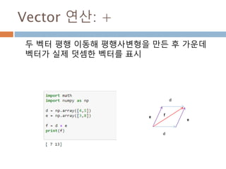
- 292. Vector 연산: + 두 벡터 평행 이동해 평행사변형을 만든 후 가운데 벡터가 실제 덧셈한 벡터를 표시 e d f e d 292
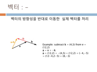
- 293. 벡터 : - 벡터의 방향성을 반대로 이동한 실제 벡터를 처리 Example: subtract k = (4,5) from v = (12,2) a = v + −k a = (12,2) + −(4,5) = (12,2) + (−4,−5) = (12−4,2−5) = (8,−3) 293
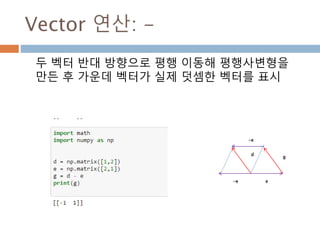
- 294. Vector 연산: - 두 벡터 반대 방향으로 평행 이동해 평행사변형을 만든 후 가운데 벡터가 실제 덧셈한 벡터를 표시 e d g -e -e 294
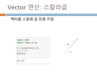
- 295. 벡터: 스칼라곱 벡터의 각 원소에 스칼라값만큼 곱하여 표시 벡터 m = [7,3] A = 3m= [21,9] 295
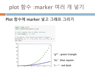
- 296. Vector 연산: 스칼라곱 스칼라 배수 만큼 벡터 내의 원소값이 커짐 d 3d 296
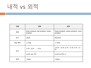
- 297. 내적과 외적 비교297
- 298. 내적 vs 외적 구분 내적 외적 명칭 Inner product, dot product, scalar product Outer product, vector product, cross product 표기 .(Dot) X(cross) 대상 벡터 n 차원 3 차원 공식 a1 b1 + a2 b2 + …. + an bn (a2 b3 – a3 b2, a3 b1 – a1 b3, a1 b2 – a2 b1) |a||b| cos 각도 |a||b| sin각도 n 결과 scalar vector 298
- 299. 스칼라곱299
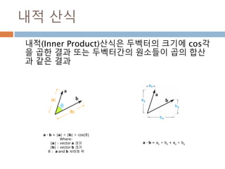
- 300. 내적 산식 내적(Inner Product)산식은 두벡터의 크기에 cos각 을 곱한 결과 또는 두벡터간의 원소들이 곱의 합산 과 같은 결과 a · b = |a| × |b| × cos(θ) Where: |a| : vector a 크기 |b| : vector b 크기 θ : a and b 사이의 각 a · b = ax × bx + ay × by 300
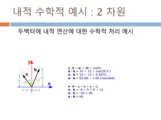
- 301. 내적 수학적 예시 : 2 차원 두벡터에 내적 연산에 대한 수학적 처리 예시 a · b = |a| × |b| × cos(θ) a · b = 10 × 13 × cos(59.5°) a · b = 10 × 13 × 0.5075... a · b = 65.98... = 66 (rounded) a · b = ax × bx + ay × by a · b = -6 × 5 + 8 × 12 a · b = -30 + 96 a · b = 66 301
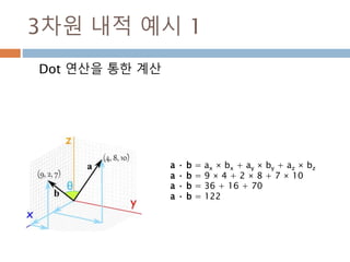
- 302. 3차원 내적 예시 1 Dot 연산을 통한 계산 a · b = ax × bx + ay × by + az × bz a · b = 9 × 4 + 2 × 8 + 7 × 10 a · b = 36 + 16 + 70 a · b = 122 302
- 303. 3차원 내적 예시 2 두벡터 사이의 각 구하기 a벡터의 크기 |a| = √(42 + 82 + 102) = √(16 + 64 + 100) = √180 b벡터의 크기 |b| = √(92 + 22 + 72) = √(81 + 4 + 49) = √134 내적 구하기 a · b = 9*4+ 2*8+ 7*10 = 36+16+70 = 122 각 구하기 a · b = |a| × |b| × cos(θ) 산식에 대입 122 = √180 × √134 × cos(θ) cos(θ) = 122 / (√180 × √134) cos(θ) = 0.7855... θ = cos-1(0.7855...) = 38.2...° 303
- 304. 내적(dot) 예시 두벡터에 대한 내적(dot) 연산은 같은 위치의 원 소를 곱해서 합산함 두벡터의 곱셈은 단순히 원소를 곱해서 벡터를 유지 304
- 305. vdot: vector 벡터(2차원)일 경우도 스칼라(dot)로 처리 305
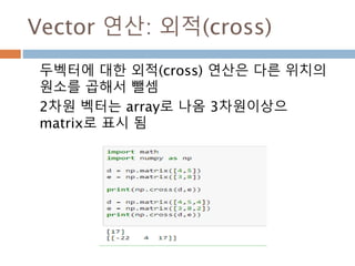
- 307. 외적 벡터 a 와 b 의 외적은 a × b 로 정의된다. 외적의 결과로 나온 벡터 c 는 벡터 a 와 b 의 수직 인 벡터로 오른손 법칙의 방향 Vector product Cross product 307
- 308. 외적 산식 : 2차원 벡터의 원소간의 cross 적을 처리 v = [a1,a2] u = [b1,b2] a1 a2 b1 b2 a1*b2 – a2*b1 Example: The cross product of a = (2,3) and b = (5,6) c = a1b2 − a2b1 = 2×6− 3×5 = −3 Answer: a × b = -3 308
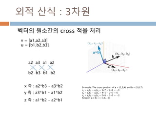
- 309. 외적 산식 : 3차원 벡터의 원소간의 cross 적을 처리 v = [a1,a2,a3] u = [b1,b2,b3] a2 a3 a1 a2 b2 b3 b1 b2 x 측 : a2*b3 – a3*b2 y 측 : a3*b1 – a1*b2 z 측 : a1*b2 – a2*b1 Example: The cross product of a = (2,3,4) and b = (5,6,7) cx = aybz − azby = 3×7 − 4×6 = −3 cy = azbx − axbz = 4×5 − 2×7 = 6 cz = axby − aybx = 2×6 − 3×5 = −3 Answer: a × b = (−3,6,−3) 309
- 310. 외적 산식예시 두벡터에 대한 외적(cross) 연산은 다른 위치의 원소를 곱해서 뺄셈 2차원 벡터는 스칼라 값으로 나옴 3차원 벡터이 상 표시 됨 310
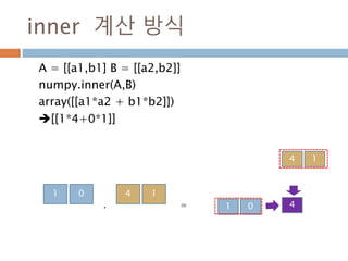
- 312. inner 계산 방식 A = [[a1,b1] B = [[a2,b2]] numpy.inner(A,B) array([[a1*a2 + b1*b2]]) [[1*4+0*1]] 1 0 4 1 1 0 4 1 4=. 312
- 313. Inner 예시 벡터의 내부 곱한 것을 더해서 값을 표현 313
- 314. dot/inner: 예시 벡터(2차원)일 경우 2차원으로 표시 314
- 315. outer A = [[a1,b1]] B = [[a2,b2]] numpy.outer(A,B) array([[a1*a2 , a1*b2][ b1*a2, b1*b2]]) [[1*4,1*1] [0*4+0*1]] 1 0 4 1 1 0 4 1 4 1 0 0 = 315
- 316. outer 예시 벡터의 내부 곱한 것을 더해서 값을 표현 첫번째 벡터의 전치와 두번째 벡터와의 Dot 연 산과 같은 결과 316
- 318. 벡터 산술연산318
- 319. Vector 연산: + 두 벡터 평행 이동해 평행사변형을 만든 후 가운데 벡터가 실제 덧셈한 벡터를 표시 e d f e d 319
- 320. Vector 연산: - 두 벡터 반대 방향으로 평행 이동해 평행사변형을 만든 후 가운데 벡터가 실제 덧셈한 벡터를 표시 e d g -e -e 320
- 321. Vector 연산: 스칼라곱 벡터를 스칼라 곱 만큼 커짐 d 3d 321
- 322. 벡터 크기322
- 323. Vector 크기 계산 벡터의 크기(Magnitude)는 원소들의 제곱을 더 하고 이에 대한 제곱근의 값 벡터의 크기는 x축의 변위와 y축의 변위를 이용 하여 피타고라스 정리 323
- 324. vector 내적324
- 325. Vector 연산: 내적(dot) 두벡터에 대한 내적(dot) 연산은 같은 위치의 원 소를 곱해서 합산함 325
- 326. vector 외적326
- 327. Vector 연산: 외적(cross) 두벡터에 대한 외적(cross) 연산은 다른 위치의 원소를 곱해서 뺄셈 2차원 벡터는 array로 나옴 3차원이상으 matrix로 표시 됨 327
- 329. 행렬이란329
- 330. 행렬 매트릭스라고도 하는데 행렬의 가로 줄을 행, 세 로 줄을 열로 표시함 330
- 331. Diagonal matrix331
- 332. 대각행렬 정사각행렬 A=(aij)(i, j=1, 2, 3,…, n)의 원소 aij가 aij=0(i≠j)을 만족시키는 행렬 A의 주대각선 위에 있는 원소(대각선원소) aij(i=j) 외의 원소 aij(i≠j)가 모두 0인 행렬 332
- 333. Identity matrix333
- 334. 항등행렬 모든 행렬과 닷 연산시 자기 자신이 나오게 하는 단위행렬 import numpy as np a = np.array([[1,0],[0,1]]) b = np.array([[4,1],[3,2]]) print(np.dot(b,a)) print(np.dot(a,b)) [[4 1] [3 2]] [[4 1] [3 2]] 334
- 335. Triangular matrix335
- 336. 삼각행렬 상삼각 행렬(Upper triangular matrix) 과 하삼각 행렬(lower triangular matrix )을 총칭하여 일컫는 말. Upper triangular matrix lower triangular matrix 336
- 337. 행렬 산술연산337
- 338. 행렬 산술연산 두 행렬의 원소별로 산술연산(+/-/*) 처리 + - * / = + - * / + - * / + - * / + - * / + - * / + - * / 1 2 3 4 5 6 1 2 3 4 5 6 + = 1+1 2+2 3+3 4+4 5+5 6+6 = 2 4 6 8 10 12 338
- 339. 행렬 산술연산 예시 행렬에 대한 산술연식은 각 원소별로 +/-/* 처리 339
- 340. 행렬의 전치(transpose)340
- 341. 행렬 전치 전치: 행렬의 행과 열을 서로 바꾸는 것. 수학책에서는 위첨자 T로 행렬 A의 전치를 나타 낸다. 121110 987 654 321 A 12963 11852 10741 T A 341
- 342. 행렬 전치 예시 파이썬은 기본 속성에서 T 변수를 제공하고 numpy 모듈에서 transpose 함수 제공 342
- 343. dot 연산343
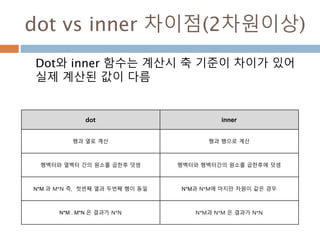
- 344. dot vs inner 차이점(2차원이상) Dot와 inner 함수는 계산시 축 기준이 차이가 있어 실제 계산된 값이 다름 dot inner 행과 열로 계산 행과 행으로 계산 행벡터와 열벡터 간의 원소를 곱한후 덧셈 행벡터와 행벡터간의 원소를 곱한후에 덧셈 N*M 과 M*N 즉, 첫번째 열과 두번째 행이 동일 N*M과 N*M에 마지만 차원이 같은 경우 N*M . M*N 은 결과가 N*N N*M과 N*M 은 결과가 N*N 344
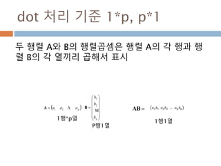
- 345. dot 처리 기준 1*p, p*1 두 행렬 A와 B의 행렬곱셈은 행렬 A의 각 행과 행 렬 B의 각 열끼리 곱해서 표시 AB 𝑎1 𝑏1 𝑎2 𝑏2 … 𝑎 𝑝 𝑏 𝑝 paaa 21A pb b b 2 1 B 1행*p열 P행1열 1행1열 345
- 346. dot 처리 기준 두 행렬 A와 B의 행렬곱셈은 행렬 A의 각 행과 행 렬 B의 각 열끼리 곱해서 표시 pnpjpp inijii nj nj mpmjmm ipijii pj pj bbbb bbbb bbbb bbbb aaaa aaaa aaaa aaaa 21 21 222221 111211 21 21 222221 111211 AB pm np nm 2 3 3 3 346
- 347. dot : 2차원 A = [[a1,b1],[c1,d1]] B = [[a2,b2],[c2,d2]] numpy.dot(A,B) array([[a1*a2 + b1*c2, a1*b2 + b1*d2], [c1*a2 + d1*c2, c1*b2 + d1*d2]) [[1*4+ 0*2, 1*1+0*2],[0*4+1*2, 0*1+1*2]] 1 0 0 1 4 1 2 2 1 0 0 1 4 1 2 2 4 1 2 2 =. 347
- 348. dot 예시 Numpy.dot 메소드 처리 348
- 349. 행렬식349
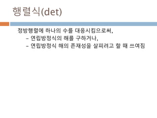
- 350. 행렬식(det) 정방행렬에 하나의 수를 대응시킴으로써, - 연립방정식의 해를 구하거나, - 연립방정식 해의 존재성을 살피려고 할 때 쓰여짐 350
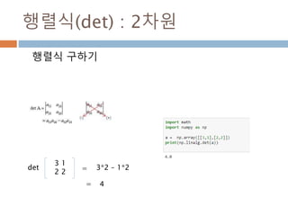
- 351. 행렬식(det) : 2차원 행렬식 구하기 3 1 2 2 det = 3*2 – 1*2 = 4 351
- 352. 행렬식(det) : 3차원 행렬식을 계산시 앞에 두 열을 뒤에 복사 후 계산 3 1 3 3 1 2 2 3 2 2 1 1 1 1 1 = 3*2*1 – 3*2*1 + 1*3*1 – 3*3*1 + 3*2*1 – 1*2*1 = 6 – 6 + 3 -9 + 6 -2 = 15 – 17 = -2 352
- 353. 행렬식(det) : 3차원 n 353
- 354. minor determinant354
- 355. 소행렬식 2차원 i번째 행,j번째 열을 제거한 부분행렬의 행렬식 : Mij 2 1 1 2 M11 2 M12 M21 -1 -1 2 1 1 부호 + 부호 – 부호 – 부호 +M22 22 355
- 356. 소행렬식 3차원 i번째 행,j번째 열을 제거한 부분행렬의 행렬식 : Mij 3 1 3 2 2 3 1 1 1 M11 2*1 -3*1 -1 M12 M13 2*1 -3*1 -1 2*1 -2*1 0 2 3 1 1 2 3 1 1 2 2 1 1 = 3M11+(-1)* 1M12 + 3M13 = -3+1+0 = -2 부호 + 부호 – 부호 + 356
- 357. 소행렬식 예시 소행렬식을 구해서 행렬식 값 비교 357
- 358. 역행렬358
- 359. 여인수(cofactor) 소행렬식을 이용한 값을 여인수를 표시 3 1 3 2 2 3 1 1 1 소행렬식 부호 결과값 m11 2 3 1 1 2-3 -1 + -1 m12 2 3 1 1 2-3 -1 - 1 m13 2 2 1 1 2-2 0 + 0 m21 1 3 1 1 1-3 -2 - 2 m22 3 3 1 1 3-3 0 + 0 m23 3 1 1 1 3-1 2 - -2 m31 1 3 2 3 3-6 -3 + -3 m32 3 3 2 3 9-6 3 - -3 m33 3 1 2 2 6-2 4 + 4 359
- 360. 수반행렬(adj) 과 여인수행렬 소행렬식으로 계산된 원소 즉 여인수로 구성된 행렬 의 전치행렬을 수반행렬이라 함 -1 2 -3 1 0 -3 0 -2 4 -1 1 0 2 0 -2 -3 -3 4 T 여인수행렬 의 전치 수반행렬 360
- 361. 역행렬(inv) – 2차원 역행렬은 수반행렬에 행렬식으로 나눗값이 됨 [[ 0.66666667 -0.33333333] [-0.33333333 0.66666667]] 1/3 * 2 -1 -1 2 역행렬 2 1 1 2 -1 A−1=1/det(A) * CT 361
- 362. 역행렬(inv) – 3차원 역행렬은 수반행렬에 행렬식으로 나눗값이 됨 [[ 0.5 -1. 1.5] [-0.5 0. 1.5] [ 0. 1. -2. ]] - 0.5 * -1 2 -3 1 0 -3 0 -2 4 역행렬3 1 3 2 2 3 1 1 1 -1 A−1=1/det(A) * CT 362
- 364. Dot 연산364
- 365. Dot 처리 기준 두 행렬 A와 B의 행렬곱셈은 행렬 A의 각 행과 행 렬 B의 각 행끼리 곱한후 덧셈을 하여 표시 pnpjpp inijii nj nj mpmjmm ipijii pj pj bbbb bbbb bbbb bbbb aaaa aaaa aaaa aaaa 21 21 222221 111211 21 21 222221 111211 AB n*m n*m n*n 두행렬의 마지막 차원이 값으면 처리가 가능하고 결과는 마지막 차원을 제외해서 구성 365
- 366. dot 행렬 n*m 행렬 일 경우 2차원으로 표시 366
- 367. dot 예시 : 2차원 a(2,2) 행렬과 b(2,2)행렬의 마지막 차수가 같으 므로 계산결과는 n*m, m*n = n*n 367
- 368. cross product368
- 369. cross 계산 방식 A = [[a1,b1],[c1,d1]] B = [[a2,b2],[c2,d2]] numpy.cross(A,B) = A.T * B array([[a1*b2 - c1*a2 , b1*d2 – d1*c2]) [[1*1- 0*4,0*2-1*2]] 1 0 0 1 4 2 1 2 1 -2= 369
- 370. Cross 행렬 n*m 행렬 일 경우 2차원으로 표시 370
- 371. Inner 연산371
- 372. inner 계산 방식 A = [[a1,b1],[c1,d1]] B = [[a2,b2],[c2,d2]] numpy.inner(A,B) array([[a1*a2 + b1*b2, a1*c2 + b1*d2], [c1*a2 + d1*b2, c1*c2 + d1*d2]) [[1*4+0*1,1*2+0*2],[0*4+1*1, 0*2+1*2]] 1 0 0 1 4 1 2 2 1 0 0 1 4 1 2 2 4 2 1 2 =. 372
- 373. Inner 예시 : 2차원 a(2,2) 행렬과 b(2,2)행렬의 마지막 차수가 같으 므로 계산결과는 out.shape = a.shape[:-1] + b.shape[:-1] 373
- 374. Inner 예시 : 3차원 a(2,3,2) 행렬과 b(2,2)행렬의 마지막 차수가 같 으므로 계산결과는 out.shape = a.shape[:-1] + b.shape[:-1] 374
- 375. outer product375
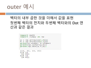
- 376. outer 두개의 벡터를 가지고 벡터 크기를 행과 열로 만드 는 함수 1차원이 이상일 경우 1차원으로 만든 후에 행렬로 만듬 1 0 4 1 1 0 4 1 4 1 0 0 = 2 2 2*2 376
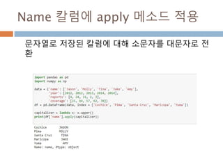
- 377. outer: 1 Out는 두개의 벡터에 대한 행렬로 구성 out[i, j] = a[i] * b[j] 377
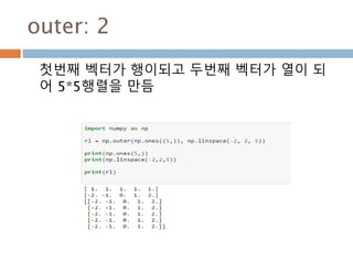
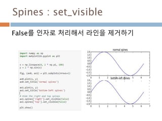
- 378. outer: 2 첫번째 벡터가 행이되고 두번째 벡터가 열이 되 어 5*5행렬을 만듬 378
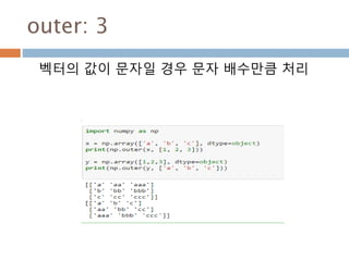
- 379. outer: 3 벡터의 값이 문자일 경우 문자 배수만큼 처리 379
- 380. tensordot380
- 381. tensordot Tensordot 함수에 axes를 0으로 줄 경우 tensor product을 연산 381
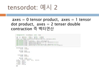
- 382. tensordot Tensordot 함수에 axes를 0으로 줄 경우 tensor product을 연산 = 1 0 0 1 4 1 2 2 1 0 0 1 4 1 2 2 4 1 2 2 4 1 2 2 4 1 2 2 = 4 2 1 2 0 0 0 0 0 0 0 0 4 2 1 2 2,2 2,2 2,2,2,2 382
- 383. tensordot: 예시 1 2차원 행렬 2개가 만나 4차원 행렬 구성 383
- 384. tensordot: 예시 2 axes = 0 tensor product, axes = 1 tensor dot product, axes = 2 tenser double contraction 즉 벡터연산 384
- 385. 대각행렬385
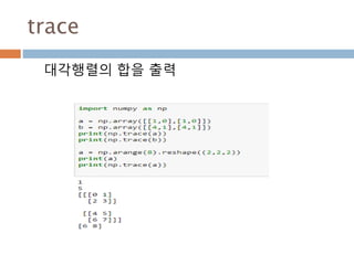
- 386. Trace : 3차원 행렬 3차원(2,2,2) 대각행렬의 합은 첫번째 차원의 1과 두번째의 마지막을 합산해서 출력 0 2 1 3 4 6 5 7 0 1 386
- 389. 행렬 이해하기389
- 390. 행렬 n개의 실수의 순서쌍에 성분별로 덧셈과 실수상수 곱을 주면[2] 이는 "nn차원" 벡터공간이라 할 수 있 고(, 벡터공간에서 벡터공간으로 가는 함수 중 덧셈 과 상수배를 보존하는 함수를 선형사상을 행렬이라 함 390
- 391. 행렬 생성 Numpy matrix 를 이용해서 행렬 생성 391
- 392. 행렬 연산하기392
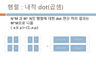
- 393. 행렬 : 내적 dot(곱셈) N*M 과 M* N인 행렬에 대한 dot 연산 처리 결과는 M*M으로 나옴 ( xij )( yij )=(∑kxikykj) a1 a2 a3 a4 b1 b2 b3 b4 a1*b1+a1*b3 a2*b2+a2*b4 a3*b1+a3*b3 a4*b2+a4*b4 = . 393
- 394. 행렬 : dot 행렬에 대한 dot 연산 처리 394
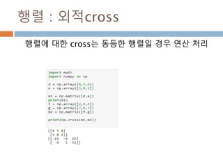
- 395. 행렬 : 외적cross 행렬에 대한 cross는 동등한 행렬일 경우 연산 처리 395
- 396. 행렬 : +/- N*M 과 N*M인 행렬에 대한 +/- 연산 처리 결과는 N*M으로 나옴 a1 a2 a3 a4 b1 b2 b3 b4 a1 +/- b1 a2 +/- b2 a3+/- b3 a4 +/- b4 = + / - 396
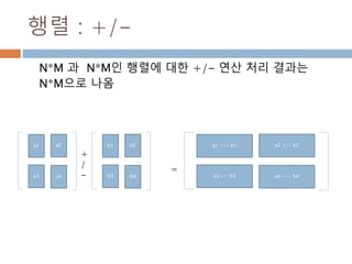
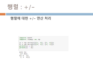
- 397. 행렬 : +/- 행렬에 대한 +/- 연산 처리 397
- 398. 행렬 : 상수 배 상수(k) 와 N*M 행렬에 대한 곱은 상수배만큼 증가 함 a1 a2 a3 a4 k* a1 k * a2 k* a3 k* a4 = k 398
- 399. 행렬 : 상수 배 행렬에 대한 k 상수만큼 원소별로 곱하는 연산 처리 399
- 400. 행렬 : 전치(transpose) N*M 행렬을 M*N을 변환하는 처리 a1 a2 a3 a4 a1 a3 a2 a4 = T 400
- 401. 행렬 : 전치(transpose) N*M 행렬을 M*N을 변환하는 방식은 T변수, transpose 메소드가 있음 401
- 402. matmul Matrix 타입일 경우 곱셈은 dot 연산과 동일한 결과를 생성함 402
- 403. Matmul: 차원계산 N*m, M*n 행렬에 따라 계산이 되지만 1차원인 경우는 행렬 계산을 처리 403
- 404. matrix_power matrix_power는 정방행렬에 대해 dot 연산을 제곱승만큼 계산하는 것 404
- 405. matrix_power: 예시 반복적인 dot 연산을 처리 405
- 407. Matrix and vector products407
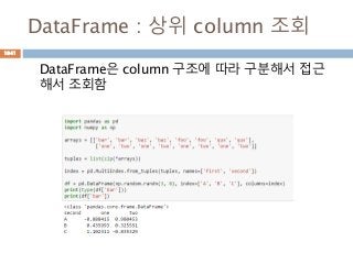
- 408. 주요 함수 선형대수에 대한 함수들 함수 설명 dot(a, b[, out]) n차원 행렬 n*m m*l에 대한 production(결과는 n*l) vdot(a, b) Vector에 대한 prodution inner(a, b) N 차원 행렬에 대한 Inner product (행렬이 동일해야 함). outer(a, b[, out]) 2개 벡터에 대해 계산 후 행렬로 표시. matmul(a, b[, out]) 두 행렬에 대한 Matrix product (dot과 동일한 결과) tensordot(a, b[, axes]) Compute tensor dot product along specified axes for arrays >= 1-D. linalg.matrix_power(M, n) Raise a square matrix to the (integer) power n. cross(a, b, axisa=-1, axisb=-1, axisc=-1, axis=None) 행렬에 대한 외적을 구함 einsum(subscripts, *operands[, out, dtype, ...]) Evaluates the Einstein summation convention on the operands. kron(a, b) Kronecker product of two arrays. 408
- 409. Decompositions409
- 410. 주요 함수 선형대수에 대한 함수들 함수 설명 linalg.cholesky(a) Cholesky decomposition. linalg.qr(a[, mode]) Compute the qr factorization of a matrix. linalg.svd(a[, full_matrices, compute_uv]) Singular Value Decomposition. 410
- 412. 주요 함수 선형대수에 대한 함수들 함수 설명 linalg.eig(a) Compute the eigenvalues and right eigenvectors of a square array. linalg.eigh(a[, UPLO]) Return the eigenvalues and eigenvectors of a Hermitian or symmetric matrix. linalg.eigvals(a) Compute the eigenvalues of a general matrix. linalg.eigvalsh(a[, UPLO]) Compute the eigenvalues of a Hermitian or real symmetric matrix. linalg.eig(a) Compute the eigenvalues and right eigenvectors of a square array. 412
- 413. Norms and other numbers413
- 414. 주요 함수 선형대수에 대한 함수들 함수 설명 linalg.norm(x[, ord, axis, keepdims]) Matrix or vector norm. linalg.cond(x[, p]) Compute the condition number of a matrix. linalg.det(a) Compute the determinant of an array. linalg.matrix_rank(M[, tol]) Return matrix rank of array using SVD method Rank of the array is the number of SVD sing ular values of the array that are greater than tol. linalg.slogdet(a) Compute the sign and (natural) logarithm of the determinant of an array. trace(a[, offset, axis1, axis2, dtype, out]) Return the sum along diagonals of the array. 414
- 415. Solving equations and inverting matrices 415
- 416. 주요 함수 선형대수에 대한 함수들 함수 설명 linalg.solve(a, b) Solve a linear matrix equation, or system of linear scalar equations. linalg.tensorsolve(a, b[, axes]) Solve the tensor equation a x = b for x. linalg.lstsq(a, b[, rcond]) Return the least-squares solution to a linear matrix equation. linalg.inv(a) Compute the (multiplicative) inverse of a matrix. linalg.pinv(a[, rcond]) Compute the (Moore-Penrose) pseudo-inverse of a matrix. linalg.tensorinv(a[, ind]) Compute the ‘inverse’ of an N-dimensional array. 416
- 418. 삼각함수 기초 Moon Yong Joon 418
- 419. 각의 종류419
- 420. 각의 종류 각은 두 선상의 사이를 말하며, 이 각에는 예각, 직각, 둔각 등이 종류가 있음 420
- 421. 직각삼각형 기본421
- 422. 직각 삼각형을 이용 삼각형이 존재할 경우 총 각이 합은 180도 이고 각 A의 값을 삼각비로 구할 수 있다 A sin(각도) 의 값은 빗변분에 높이 즉 b/c cos(각도) 의 값은 빗변분에 높이 즉 a/c tan(각도) 의 값은 빗변분에 높이 즉 b/a 422
- 423. 직각삼각형 예시423
- 424. 삼각형을 이용 : 빗변 구하기 밑변과 높이를 알면 피타고라스 정리에 따라 빗 변을 구할 수 있다. 424
- 425. 삼각형을 이용 : 높이와 밑변 하나의 각과 빗변을 알고 있을 경우 빗변*sin()으 로 높이, 빗변*cos()으로 밑변을 구하기 425
- 426. 피타고라스 정리426
- 427. 피타고라스 정리 이용하기 밑변의 제곱과 높이이 제곱은 빗변의 제곱과 동 일 A 대신 rcosø B 대신 rsinø r값을 1로 전환하면 427
- 428. 피타고라스 정리 밑변 3, 높이 4 일 경우 빗변은 5가 됨 428
- 430. 원을 이용한 삼각함수430
- 431. 원을 이용한 삼각함수 정의 xy 좌표평면에서 반지름의 길이가 r인 원을 그리 고 임의의 점을 P일 경우 OP가 이루는 각에 대해 한가지 값을 결정 반지름이 1인 경우 431
- 432. 원을 이용한 정의 예시 선분은 sqrt(3**2 + 4**2)=5가 나오고 이를 이 용해서 각 ø 에 대한 삼각함수 값을 하나로 산출 432
- 433. 삼각함수 표433
- 434. 삼각함수 표 x축은 반지름*코사인 각도, Y축은 반지름*사인 각도로 원위의 점의 좌표를 알 수 있음 434
- 435. RIDAIAN & DEGREE Moon Yong Joon 435
- 437. degrees와 radians 변환 기준 단위원을 이용하여 degrees와 radians 변환 Degrees와 Radians 변환 규칙 437
- 438. degree와 radian 변환438
- 439. degrees와 radians 2π는 360도, 1radian은 57.3도 439
- 440. degrees와 radians: 변환 90, pi/2를 변환해보면 아래와 같다 440
- 441. radians <-> degrees : numpy np.deg2rad, np.rad2deg를 이용해서 radians 또는 degree로 전환 Π와 180도에 대한 값 전환 441
- 442. radians -> degrees : numpy np.degrees를 이용해서 radians 값을 degree 로 전환 np.degrees(radian, 출력) 442
- 443. degrees-> radians : numpy np.radians를 이용해서 degree 값을 radian로 전환 np.radians(radian, 출력) 443
- 444. 기본 삼각함수 Moon Yong Joon 444
- 445. cosine445
- 446. cosine 그래프 수평선의 길이를 코사인 값을 표시. 446
- 447. cosine 그래프 수평선의 길이를 코사인 값을 표시. 447
- 448. cosine 그래프 : numpy 수평선의 길이를 코사인 값을 표시. 448
- 449. cosine 그래프 수평선의 길이를 코사인 값을 표시. 449
- 450. sine450
- 451. sine함수 sine 함수에 radians을 넣어 값을 계산 451
- 452. sine 그래프 수직선의 길이를 코사인 값을 표시. 452
- 453. sine 그래프 : numpy 수직선의 길이를 코사인 값을 표시. 453
- 454. sine 그래프 수평선의 길이를 사인 값을 표시. 454
- 455. tangent455
- 456. tan 함수 tangent 함수에 radians을 넣어 값을 계산 456
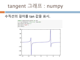
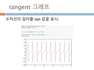
- 457. tangent 그래프 수직선의 길이를 tan 값을 표시. 457
- 458. tangent 그래프 : numpy 수직선의 길이를 tan 값을 표시. 458
- 459. tangent 그래프 수직선의 길이를 tan 값을 표시. 459
- 460. 삼각함수 각의 변환 Moon Yong Joon 460
- 461. 각의 변환461
- 462. 각의 변화를 알아보기 각은 n*π/2 + θ 또는 90n + θ으로 변환해서 각의 위치에 따라 삼각함수를 변환 1. 나오는 각을 n*π/2 + θ 또는 90n + θ, 이때 n은 정수 이면 0< θ < π/2 , 0 < θ <90 2. n이 짝수이면 변하지 않지만 홀수이면 sin-> cos, cos-> sin, tan-> cot로 변환 3. 몇 사분면의 각이냐 에 따라 부호가(+,-)로 변환됨 1사분면 2사분면 3사분면 4사분면 sin + + - - cos + - - + tan + - + - 462
- 463. 삼각함수 사분면 부호 삼각함수의 사분면 위치에 따른 결과 값에 대한 부호 표시 463
- 464. 각의 변화 : 짝수 각은 n*π/2 + θ 또는 90n + θ에서 n이 짝수일 때는 부호만 변함 n=0, 동일함수, 4사분면 n=2, 동일 함수, 2사분면 sin(-x) = -sin(x) sin(π -x) = sin(x) cos(-x) = cos(x) cos(π-x) = -cos(x) tan(-x) = - tan(x) tan(π-x) = -tan(x) 464
- 465. 각의 변화 : 짝수예시 각은 n*π/2 + θ 또는 90n + θ에서 n이 짝수일 때는 부호만 변함 465
- 466. 각의 변화 : 홀수 각은 n*π/2 + θ 또는 90n + θ으로 n이 홀수일 경우 삼각함수가 변함 n=1, 다른 함수, 1사분면 n=3, 동일 함수, 3사분면 sin(π/2 -x) = cos(x) sin(3π/2 -x) = -cos(x) cos(π/2-x) = sin(x) cos(3π/2-x) = -sin(x) tan(π/2-x) = cot(x) tan(3π/2-x) = cot (x) 1 466
- 467. 각의 변화 : 홀수 예시 각은 n*π/2 + θ 또는 90n + θ으로 n이 홀수일 경우 삼각함수가 변함 467
- 468. π/2 :예각468
- 469. 삼각함수 변화 : π/2 각 A가 120도 일 경우는 π/2(90)+30의 값을 가지므로 sin일 경우 cos, cos일 경우는 –sin 으 로 바뀜 r a b A=120도 B=30도 469
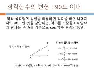
- 470. 삼각함수의 변형 : 90도 이내 직각 삼각형의 성질을 이용하면 직각을 빼면 나머지 각이 90도인 것을 감안하면, 각 B를 기준을 sin 함수 의 결과는 각 A를 기준으로 cos 함수 결과와 동일 A B cos(A) = sin(B), sin(B) = cos(A) , tan(B) = cot(A) 와 동일 각 A + 각 B = 90도 각 B로 삼각함수 처리 470
- 471. 삼각함수의 변형 예시 π/2 – 예각에 대한 삼각함수 계산 471
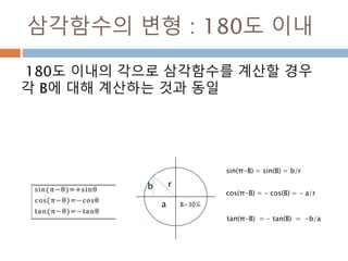
- 472. 삼각함수의 변형 : 180도 이내 180도 이내의 각으로 삼각함수를 계산할 경우 90도 + 나머지 각으로 삼각함수를 계산할 수 있 음 r a b A=120도 B=30도 sin(A) = cos(B) = b/r cos(A) = - sin(B) = - a/r tan(A) = - cot(B) = -b/a 472
- 473. 삼각함수의 변형 예시 π/2 + 예각에 대한 삼각함수 계산 473
- 474. π 와 예각 연산474
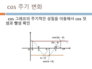
- 475. Sin 주기 변화 sin 그래프의 주기적인 pi 와 2pi 배수 단위로 동일한 값을 처리 성질을 이용 475
- 476. cos 주기 변화 cos 그래프의 pi 와 2pi 배수 단위로 동일한 값 을 처리 성질을 이용 476
- 477. 삼각함수 변화 : π - 예각 180도 이내의 각으로 삼각함수를 계산할 경우 각 B에 대해 계산하는 것과 동일 r a b B=30도 sin(π-B) = sin(B) = b/r cos(π-B) = - cos(B) = - a/r tan(π-B) = - tan(B) = -b/a 477
- 478. 삼각함수 변화 : π + 예각 각 A가 120도 일 경우는 π(180)+30의 값을 가 지므로 sin일 경우 sin, cos일 경우는 –cos 으로 바뀜 r a b A=210도 B=30도 478
- 479. 2π 와 예각 연산479
- 480. 삼각함수 변화 : 2π - 각 A가 360도 일 경우는 2π(360)-30의 값을 가지므로 sin일 경우 -sin, cos일 경우는 –cos 으 로 바뀜 r a b A=360도 B=30도 480
- 481. 삼각함수 변화 : 2π + 삼각함수가 2 π 단위로 변경시는 항상 기존 예 각을 구하는 것도 동일한 값을 같는다. r a bA=360도 B=30도 481
- 482. 삼각함수 덧셈과 뺄셈공식 Moon Yong Joon 482
- 483. Sin 함수의 덧셈483
- 484. Sin 함수 덧셈 두개의 각을 sin으로 덧셈을 할 경우 sin함수별 로 덧셈과는 차이가 발생 r a b t s sin(α+ β) = sin(α) cos(β) + cos(α) sin(β) = a/r * b/s + b/r * t/s sin(α) cos(β) = a/r * b/s cos(α) sin(β) = b/r * t/s sin(α) = a/r , sin(β) = t/s 484
- 485. Sin 함수 덧셈 예시 sin 함수 두개의 각을 더할 경우 아래의 공식으 로 계산 485
- 486. Sin 함수의 뺄셈486
- 487. Sin 함수 뺄셈 예시 sin 함수 두개의 각을 뺄 경우 아래의 공식으로 계산 Cos 90이 0값이 아니라도 아 주 작은 값이라 무시 487
- 488. cos 함수의 덧셈/뺄셈488
- 489. cos함수 덧셈 예시 cos 함수 두개의 각을 더할 경우 아래의 공식으 로 계산 489
- 490. cos함수 뺄셈 예시 cos 함수 두개의 각을 뺄 경우 아래의 공식으로 계산 490
- 492. 역수492
- 493. 역수 어떤 수의 역수(逆數, 영어: reciprocal) 또는 곱셈 역원(- 逆元, 영어: multiplicative inverse)은 그 수와 곱해서 1, 즉 곱셈 항등원이 되는 수를 말한다. x의 역수는 1/x 또는 x -1로 표기한다. 곱해서 1이 되는 두 수를 서로 역 수 493
- 494. 역수 구하기494
- 495. 역수 구하기 Python에는 역수에 대한 함수가 없어 역수 공식 에 따라 계산 495
- 496. 삼각함수*역수 = 1 삼각함수 * 역수 = 1인지 확인 496
- 498. 역함수 사용하기498
- 499. 역함수 함수의 정의역과 치역을 바꾸서 함수를 만드는 것을 역함수라고 함 499
- 500. 삼각함수의 역함수 삼각함수의 역함수가 역삼각함수 이름 표기법 정의 정의역 치역 아크사인 y = arcsin x 또는 y = sin-1 x x = sin y −1부터 +1 −π/2 ≤ y ≤ π/2 아크코사인 y = arccos x 또는 y = cos-1 x x = cos y −1부터 +1 0 ≤ y ≤ π 아크탄젠트 y = arctan x 또는 y = tan-1 x x = tan y 모든 실수 −π/2 < y < π/2 아크코탄젠트 y = arccot x 또는 y = cot-1 x x = cot y 모든 실수 0 < y < π 아크시컨트 y = arcsec x 또는 y = sec-1 x x = sec y −∞부터 −1과 1부 터 ∞ 0 ≤ y < π/2 or π/ 2 < y ≤ π 아크코시컨트 y = arccsc x 또는 y = csc-1 x x = csc y −∞부터 −1과 1부 터 ∞ −π/2 ≤ y < 0 or 0 < y ≤ π/2 500
- 501. arcsine501
- 502. arcsine 삼각함수의 역함수가 역삼각함수 이름 표기법 정의 정의역 치역 아크사인 y = arcsin x 또는 y = sin-1 x x = sin y −1부터 +1 −π/2 ≤ y ≤ π/2 502
- 503. arcsine : numpy 삼각함수의 역함수가 역삼각함수 이름 표기법 정의 정의역 치역 아크사인 y = arcsin x 또는 y = sin-1 x x = sin y −1부터 +1 −π/2 ≤ y ≤ π/2 503
- 504. arcsine : numpy 그래프 삼각함수의 역함수가 역삼각함수 504
- 505. arccosine505
- 506. arccosine : numpy 삼각함수의 역함수가 역삼각함수 이름 표기법 정의 정의역 치역 아크코사인 y = arccos x 또는 y = cos-1 x x = cos y −1부터 +1 0 ≤ y ≤ π 506
- 507. arccosine : numpy 그래프 삼각함수의 역함수가 역삼각함수 507
- 508. arctangent508
- 509. 삼각함수의 역함수 삼각함수의 역함수가 역삼각함수 이름 표기법 정의 정의역 치역 아크탄젠트 y = arctan x 또는 y = tan-1 x x = tan y 모든 실수 −π/2 < y < π/2 509
- 511. 지수함수 기초 Moon Yong Joon 511
- 512. 지수 함수512
- 513. 지수 함수란? x에 대한 지수함수(exponential function). a>0 커야 실수 값으로 처리되며 a=1일 경우 항 상 1인 상수가 됨 임의의 실수 x에 대해 함수 513
- 514. 임의의 실수 x에 대해 y = ex 5의 지수는 e5이고 약 148.413과 같습니다 자연지수함수 ex에서 e는 약 2.71828인 자연 로그의 밑이고, x는 입력하는 값으로 구성된 함수 514
- 515. 지수함수 그래프 지수함수는 a>0 크면 우상향 그래프 0<a<1 이 면 우하향 그래프가 됨 515
- 516. 지수 법칙516
- 517. 지수 법칙 동일한 상수의 곱일 경우 지수는 덧셈, 동일한 상수의 제곱에 제곱은 지수끼리 곱셈 처리 * =1 역수 517
- 518. 지수 법칙 : exp 자연로그에 대한 제곱승 계산 518
- 519. 지수 법칙 : exp 그래프 복리 이자, 방사선 감소 또는 모집단 성장과 같 이 일정한 지수 요인에 의해 증가 또는 감소하는 양을 모형화하는 데 자주 사용 519
- 520. 로그함수 기초 Moon Yong Joon 520
- 521. 로그함수란521
- 522. 로그함수 정의 어떤 수를 나타내기 위해 고정된 밑을 몇 번 곱하 여야 하는지를 나타내는 함수이면서 지수함수의 역함수가 로그함수 522
- 523. 로그함수 규칙 밑과 진수, 로그함수의 관계 523
- 524. 상용로그 밑(Base)이 10 인 로그를 상용로그(상용대수: Common Logarithm)라고 함 524
- 525. 상용로그 : log10 밑(Base)이 10 인 로그를 상용로그(상용대수: Common Logarithm)라고 함 525
- 526. 자연로그 밑이 e (오일러 상수: 약 2.718) 인 로그를 자연 로그(자연대수: Natural Logarithm) 정의 기초성질 526
- 527. 자연로그 : log 밑이 e (오일러 상수: 약 2.718) 인 로그를 자연 로그(자연대수: Natural Logarithm) 527
- 528. 로그함수 성질528
- 529. 로그함수의 성질 1 로그의 진수가 1인 경우 는 0, 로그의 진수와 밑 이 같으면 1 양변에 밑을 a로 하는 log 로 곱하면 = 529
- 530. 로그함수의 성질1 : 예시 Numpy.log10는 상용로그, numpy.log는 자연 로그로 처리 530
- 531. 로그함수의 성질 2 : 지수의 곱 로그의 진수가 M*N일 경우 log의 덧셈으로 분리 log100 = log10+log10 = 2 531
- 532. 로그함수의 성질 2: 지수의 나누기 로그의 진수가 M/N일 경우 log의 나누기으로 분 리 log100/100= log100- log100 = 1 ax =M, ay = N 이면 532
- 533. 로그함수의 성질 2: 상수 배 로그의 진수가 M*N일 경우 log의 상수배를 밖으 로 분리 log10**2= 2 log10 = 2 533
- 534. 로그함수의 성질 2 : 예시 Numpy.log10으로 사용로그를 처리 534
- 535. 밑의 변환 로그에 대해 밑을 c로 하는 로그 함수로 변환이 가능 log 10 100 = log 10 100 / log 10 10 = 2/1 = 1 535
- 536. 급수 기초 Moon Yong Joon 536
- 538. 급수(級數,series, ∑an) 수학에서의 급수는 수열 a_1, a_2, a_3, ... , a_na1,a2,a3,...,an까지 주어졌을 때 이것들을 다 더 해 a_1+a_2+a_3+...+a_n, a1+a2+a3+...+an로 나타낸 것, 즉 수열의 합을 의미한다. 급수의 예는 등차수열, 등비수열의 합, 자연수의 거 듭제곱의 합 등이 있다 538
- 539. 급수의 표현 1 Σ 는 일반항 식을 가지고 시작항과 마지막 항까 지의 합을 표시하는 수학식 539
- 540. 급수의 표현 2 급수는 연속된 숫자들이 합을 구하는 것에 대한 일반식과의 비교 540
- 541. 급수의 성질541
- 542. 급수의 일반적인 성질 급수간의 계산을 위해 필요한 산식 배분의 가능 상수는 n번 덧셈 상수는 Σ 밖으로 배출 542
- 543. 급수의 일반적인 성질 급수 내에 곱과 나눗셈에 대해서는 Σ를 배분할 수 없음 급수의 나눗셈 급수의 곱 543
- 544. 유한급수 , 무한급수 수열의 모든 항을 더한 것이다. 항의 개수가 유한 한 유한 급수(有限級數, finite series)와 항의 개수가 무한한 무한 급수(無限級數, infinite series)로 분류 됨 유한 급수(有限級數, finite series) 무한 급수(無限級 數, infinite series) 544
- 545. 등차급수545
- 546. 등차급수 등차급수[ arithmetic series , 等差級數 ] 산술급수(算術級數)라고도 한다. 등차수열을 이 루고 있는 것을 말 함 급수 a1+a2+a3+…+an+…에서 an=an-1+d(n=2,3,…) 인 관계식 급수로 표시 546
- 547. 등비급수547
- 548. 등비급수 기하급수(幾何級數)라고도 한다. 급수 a1+a2+a3+…+an+…에 있어 an=arn-1 (n=2,3,…)인 관계식 548
- 549. 수열 기초 Moon Yong Joon 549
- 551. 등차수열 초기값을 가지고 동일한 값으로 숫자가 증가되 는 수열 일반항 551
- 552. 공차 등차수열에서 연속하는 두 수의 차이를 공차(公 差. Common difference)라고 한다. 보통 d로 표 시한다 552
- 553. 등차 수열의 합553
- 554. 등차 수열의 합 : 등차급수 등차급수( arithmetic series)는 등차수열의 합이 다. 초항부터 n번째 항까지의 합Sn는 다음과 같은 공식으로 나타난다 554
- 555. 등차 수열의 합의 산식 하나의 등차수열과 이 등차수열을 역으로 변환해 서 더하며 동일한 패턴이 값이 나오고 이를 다시 하나(2로 나눔)로 만들면 합산 값이 됨 등차수열을 역순으로 만들고 합산 하면 동일한 결과를 가진 패턴이 나옴 패턴 찾을 것을 2로 나누면 수열 의 합이 계산됨 555
- 556. 등차수열의 합 1 첫번째항과 마지막 항을 알고 둘 사이의 개수를 알 경우 556
- 557. 등차수열의 합 2 첫째항과 공차만 있을 경우 처리하는 방식 첫번째항(a), 마지막항( a*(n-1)*d)을 더해서 총 개수만큼 곱하고 이를 2로 나눈면 됨 557
- 558. 초기값이 중간부터 오는 경우 초기값이 중간부터 올 경우 계산하는 급수 초기값 a= 11 이고 공차 d = 1이면서 개수 n = 5 인 급수를 계산하기 11+ 12 + 13 + 14+ 15 산식 = na + n/2(n-1)d = 5*11 + 5/2(5-1) *1 = 55 + 10 = 65 558
- 560. 등비수열 초기값을 가지고 동일한 값으로 곱해서 얻어지 는 수열 일반항 560
- 561. 공비 등비수열에서 연속하는 두 수의 차이를 공비 ( Common ratio)라고 한다. 보통 r로 표시한다 561
- 562. 등비 수열의 합562
- 563. 등비 수열의 합 : 등비급수 a1부터 an까지 더한 합인 등비급수( geometric series) 또는 기하급수 Sn은 다음과 같이 구할 수 있다. 563
- 564. 등비수열의 합 첫번째과 등비를 알 경우 계산이 가능 단 등비가 1일 경우는 첫번째 항에 개수만큼 곱하면 됨 동일한 값으로 처리를 위해 등 비로 양변을 곱하고 빼면 564
- 565. 등비수열의 합 예시 등비수열의 Sn합은 an(다음항) – a(초항)/(등비- 1)로 처리 S4 = 2+4+8+16 = 30 S5는 다음항 a5 = 32 S3 = 32 – 2/(2-1) r = 2 a1 = 2 a2 = 4 a3 = 8 a4 = 16 565
- 566. 등비수열의 합 예시 첫번째과 등비를 알 경우 계산이 가능 단 등비가 1일 경우는 첫번째 항에 개수만큼 곱하면 됨 566
- 567. 수열의 극한 Moon Yong Joon 567
- 568. 급수와 극한568
- 569. 수열의 극한 수열의 극한(數列-極限, limit of a sequence) 은 수열이 한없이 가까워지는 값이다. 직관적으로, 수열 (an)이 수렴(收斂, convergent) 한다는 것은 n이 커짐에 따라 an이 어떤 고정된 값 a에 한없이 가까워지는 것을 뜻한다. 이때 a를 수열 {an}의 극한이라고 한다. 수열이 수렴하지 않으면 발산(發散, divergent)한 다고 한다. 569
- 570. 부분합 급수 무한급수 중에 특정 위치까지의 유한개의 항에 대한 합을 나타내는 급수 570
- 571. 무한수열과 극한 무한수열 {an}에서 n이 무한히 커짐에 따라 an이 일정한 값 α에 한없이 가까워지면, α를 그 수열 의 극한 또는 극한값(limit value) 부분합 n이 한없이 커진다: n-> 무한대 an 한없이 ά에 가까워진다 : an-> ά 무한수열의 극한값 ά이다 -> 571
- 572. 수렴과 발산572
- 573. 수렴 한 점으로 모인다는 뜻. 보통 의견 수렴이라든지 여론 수렴 등등으로 해서 한 점에 모인다는 의미 로 사용하는 경우가 많은데, 이 뜻을 수학으로 빌 려와서 여러 값이 기어코야 한 값으로 모이게 되 었다는 의미로 사용한다. 즉 x가 a에 한없이 가까워지거나 한없이 커지거 나 작아지면 f(x)도 어디로 한없이 가까워진다는 뜻. 573
- 574. 발산 수렴하지 않으면 발산한다. 수열이 계속 커지는 양의 무한대로 발산, 수열이 계속 작아지는 음의 무한대로 발산이 있다. 574
- 575. 수열 극한의 기본 성질575
- 576. 극한의 기본 성질 수열이 수렴할 때 이 기본 성질이 사용됨 576
- 578. 함수의 극한 기초 Moon Yong Joon 578
- 579. 함수의 극한579
- 580. 함수의 극한 함수의 극한( limit of a function)은 어떤 점에 가까이 다다름에 따른, 함수의 행태에 대한 개념 580
- 581. 좌극한값/우극한값 그래프에서 좌측과 우측에서 접근하는 것에 따라 값을 구분 581 좌극한우극한
- 582. 함수의 연속 함수f(x)가 정의역의 한점 a에 대해 다음 세 조건 을 만족하면 함수 f(x)는 x=a에서 연속되므로 연 속함수 582
- 583. 함수의 극한의 수렴583
- 584. 함수의 극한의 수렴 함수의 극한은 독립 변수가 일정한 값에 한없이 가까워질 때, 함숫값이 한없이 가까워지는 값이 존재하면 수렴한다고 함 584
- 585. 함수의 극한의 성질585
- 586. 함수 극한의 성질 수렴하는 함수들이 존재할 때 함수들의 사칙연산 을 처리할 수 있음 586
- 588. 할선과 접선588
- 589. 할선 할선(割線, 가름선)은 원 또는 곡선과 두 개 이상 의 점에서 만나 그 원이나 곡선을 자르는 직선 589
- 590. 접선 접선(接線)은 곡선 L의 두 점 A와 B로 정의되는 할선AB에 서 점 B가 곡선을 따라 점 A에 한없이 가까워 질때, 이 새 로운 선을 곡선L의 A에서 만나는 접선이라 한다 590 A 점과 만나 는 점을 접선 이고 이 점을 접점이라고 함
- 591. 기울기 기울기(slope)는 직선이 기울어진 정도를 나타내 는 수 591
- 592. 평균변화율: 할선기울기592
- 593. 평균변화율 : 할선 y=f(x) 에서 A(a,f(a)), B(b,f(b))두 정점이 있을 때 두 점간의 변화를 계산하면 곡선 위의 두 점의 기울기를 의미 593 일때 라고 두면
- 594. 미분계수: 접선기울기594
- 595. 순간변화율/미분계수 평균변화율의 극한을 취하여 함수 f(x)의 특정 지 점 x 에서 변화량 Δx가 0으로 수렴할 때의 변화 율을 순간변화율 즉 미분계수 595
- 596. 순간변화율(미분계수) 흐름 접점의 기울기를 구하기 위한 흐름 596 평균변화율 구하기 미분 순가변화율 구하기
- 597. 순간변화율(미분계수)의 그래프 B점에서 A점으로 이동하면 한점에서 만나는 접선 이 됨 597
- 598. 미분 가능598
- 599. 미분가능한 함수 : differentiable function 미분은 함수 f(x)의 순간변화율을 계산하는 과정 이다. f(x)에서 미분계수 f'(a) 가 존재할 때 미분 가능이 라고 한다. 정의역의 모든 점에서 미분가능한 함수이다. 즉, 모든 곳에서 수직이 아닌 접선을 그릴 수 있다 는 것이다 599
- 600. 미분가능 함수 f가 점 x0에서 미분가능하다는 건 그 점에서 의 미분, 즉 평균변화율의 극한이 존재하는 것으 로 정의된다 600
- 601. 도함수601
- 602. 미분계수와 도함수 차이 미분계수는 특정한 점 (a, f(a))에서 접선의 기울기를 의미하고 도함수는 임의의 점(x, f(x))에서의 접선의 기울기를 의미 602 x=1에서 미분계수는 f’(1) = 6 f(x)의 도함수는 f’(x) = 3x+3 도함수에 특정값이 들어가면 미분계수를 구할 수 있음
- 603. 도함수 미분(微分)은 함수의 순간변화율을 구하는 계산 과정 이고 함수를 미분하여 생성되는 함수를 도함수 즉 미분계수의 일반화 603 변화률에 대해 limit(극한) 을 지정하면
- 604. 이계도함수604
- 605. 변곡점 변곡점(point of inflection)은 위로 볼록인 상태 에서 오목인 상태 또는 위로 오목인 상태에서 볼 록인 상태로 변하는 점 605
- 606. 이계 도함수 이계도함수란 도함수의 도함수라는 의미로서, 본 함수를 2번 미분하여 얻은 도함수. 함수 f(x)의 도 함수 f’(x)가 미분이 가능하면 f’(x)의 도함수를 이 계도함수 f’’(x) 606
- 607. 미분 기본 공식 1607
- 608. 미분의 기본 공식 : 1 상수의 미분, 실수배 미분, 함수의 미분에 대한 일 반 공식 608
- 609. 상수미분 상수의 미분은 실제 0이 됨 609
- 610. 실수배 미분 c라는 실수배를 가진 함수의 미분에서 실수배는 미분에 영향을 미치지 않는다 610
- 611. 함수의 미분 n 이 자연수일 경우 xn의 미분은 nxn-1 611
- 612. 미분 기본 공식 2612
- 613. 미분의 기본 공식 : 2 합과 차의 미분, 곱의 미분 613
- 614. 합과차의 미분 두함수 합에 대한 미분은 각 함수의 미분에 합과 같다 614
- 615. 곱의 미분 두 함수 곱에 대한 미분은 f(x) 함수 미분과 g(x) 함수의 곱 + f(x)함수와 g(x)함수 미분의 곱과의 합과 같다 615
- 617. 부정적분617
- 618. 부정적분 미분의 역연산으로서 정의되는 부정적분 부정적분(不定積分,indefinite integral)은 (모든) 역 도함수를 구하는 연산이다. 함수 f(x)가 F(x)의 미분 이면, F(x)는 f(x)의 역도함수이다. 618
- 619. 정적분619
- 620. 정적분: definite integral 리만 적분에서 다루는 고전적인 정의에 따르면 실수 의 척도를 사용하는 측도 공간에 나타낼 수 있는 연 속인 함수 f(x)에 대하여 그 함수의 정의역의 부분 집 합을 이루는 구간 [a, b] 에 대응하는 치역으로 이루 어진 곡선의 리만 합의 극한을 구하는 것이다. 이를 정적분(定積分, definite integral)이라 한다. 620
- 621. 8.확률과 통계 기초 Moon Yong Joon 621
- 622. 기호 표기법 Moon Yong Joon 622
- 623. 평균 표준편차 분산 기호623
- 624. 평균 표준편차 분산 기호 평균 표준편차 분산 기호 624
- 626. 평균 산식626
- 627. 산출평균: arithmetic mean 주어진 값들을 더해서 총 개수로 나누는 값 627
- 628. 기하평균: geometric mean 복수개의 수치의 곱을 수치의 개수로 제곱근을 취해서 산 출되는 평균값 - 인구성장률, 투자이률 등 성장률 평균 산출시 사용 628
- 629. 조화평균 수학에서 조화 평균(調和平均)은 주어진 수들의 역수의 산술 평균의 역수, 평균적인 변화율을 구 할 때에 주로 사용된다. 실수 a1, ..., an이 주어졌을 때, 조화 평균 H는 629
- 630. 중앙값630
- 631. 중앙값: median 중앙에 위치하는 값은 어떤 주어진 값들을 크기 의 순서대로 정렬했을 때 가장 중앙에 위치하는 값 n개의 값이 주어질 때 n이 홀수이면 (n+1)/2 번째 값 n이 짝수이면 n/2 번째 값과 n/2+1번째 값의 평균 631
- 632. 최빈값632
- 633. 최빈값: mode 가장 많이 관측되는 수는 주어진 값 중에서 가장 자주 나오는 값 {1,2,3,4,4,4,5} 주어질 때 최빈값은 4이다 633
- 634. 사분위수634
- 635. 사분위수 데이터 표본을 4개의 동일한 부분으로 나눈 값 1사분위수 2사분위수 3사분위수 4사분위수 중앙값 635
- 636. 평균/중간값/최빈값 예시636
- 637. 평균/중간값/최빈값 : statistics 평균/중간값/최빈값 구하기 637
- 638. 평균/중간값/최빈값 : numpy 평균/중간값/최빈값 구하기, scipy.stats 내의 mode 연산으로 최빈값을 찾아야 함 638
- 639. 분산 기초 Moon Yong Joon 639
- 640. 분산 정의640
- 641. 분산 : population variance 분산은 편차(값 – 평균)을 제곱해서 n(전체 개수) 로 나누어서 값을 구함. 전체집단이라 가정할 경 우 계산 641
- 642. 분산 : variance 분산은 편차(값 – 평균)을 제곱해서 n(전체 개수) 로 나누어서 값을 구함. 전체 중에 일부인 표본공 간이라 가정할 경우 계산 642
- 643. 분산 : statistics643
- 644. pvariance 평균에서 얼마나 떨어져 있는지 구하기 644
- 645. variance 평균에서 얼마나 떨어져 있는지 구하기 645
- 646. variance/pvariance 평균에서 얼마나 떨어져 있는지 구하기 646
- 647. 분산 :numpy647
- 648. variance Numpy.var는 sta.pvariance와 동일한 처리 648
- 649. 표준편차 기초 Moon Yong Joon 649
- 650. 표준편차650
- 651. Standard deviation variance에 대한 표준편차 651
- 652. 표준편차:statistics652
- 656. 표준편차 : numpy656
- 657. std variance에 대한 표준편차이며 statistics.pstdev와 동일한 결과 657
- 658. 공분산 기초 Moon Yong Joon 658
- 659. 공분산(Covariance)659
- 660. 공분산(Covariance) 공분산이라 하면 분산과는 다르게 하나의 변수 가 아닌 두 변수 사이의 관계를 나타냄 660
- 661. 공분산 : numpy 두 변량간의 공분산을 구하는 함수인 cov를 이 용 파라미터에 ddof =0 을 인수를 넣고 처리 661
- 662. 상관계수 기초 Moon Yong Joon 662
- 663. 상관계수663
- 664. 상관계수 공분산이라 하면 분산과는 다르게 하나의 변수가 아 닌 두 변수 사이의 관계를 나타냄 -1<= r <= 1 사이의 값 664
- 665. 상관관계 정도 -1<= r <= 1 사이의 값으로 상관관계 정도를 나타냄 665
- 666. 상관계수 : numpy 두 변량간의 상관 관계를 나타내는 계수 파이썬은 기본이 n으로 처리되므로 (n-1)로 처리하 려면 ddof =1 을 인수로 넣어야 n-1로 처리된다. 666
- 667. 경우의 수 기초 Moon Yong Joon 667
- 668. 경우의 수668
- 669. 경우의 수 (number of cases) 경우는 수는 사건에서 일어날 수 있는 경우의 가 짓수(원소의 개수)를 말하며, 합의 법칙과 곱의 법칙에 따라 경우의 수를 계산 같은 조건에서 여러 번 할 수 있는 실험이나 관찰로 얻어진 결과를 말한다. 즉, 어떤 실험이나 관찰에서 주어진 경우를 만족하는 경우의 집합 사건 시행 실험이나 관찰을 하는 행위 669
- 670. 합의 법칙 합의 법칙은 두 사건 A,B가 동시에 일어나지 않을 때 각각의 사건이 일어날 경우의 수를 서로 더해서 구하 는 경우 사건 A가 일어나는 경우의 수 : m 사건 B가 일어나는 경우의 수 : n 사건 A 또는 B가 일어날 경우의 수 = m+n 670
- 671. 곱의 법칙 곱의 법칙은 두 사건 A,B가 동시에(연달아서) 일어날 때 각각의 사건이 일어날 경우의 수를 서로 곱해서 구하는 경우 사건 A 가 일어나는 경우의 수 : m 사건 B가 일어나는 경우의 수 : n 사건 A와 사건 b가 동시에 일어날 경우의 수 : m*n 671
- 672. 곱의 법칙:데카르트 곱 집합 A의 원소와 집합 B의 원소인 순서쌍을 만드 는 집합 집합 A={a,b}, B= {1,2} 일때 A*B = {(a,1),(a,2),(b,1),(b,2)} 즉 2*2 = 4 672
- 673. 합/곱의 법칙 구별 동시에 일어나는 사건을 경우 별개의 두 사건이 모두 발 생하는 것(곱의 법칙)이고, 별개의 두 사건이 있는 경우 둘다 일어나지 않아도 상관없는 것(합의 법칙)임 독립사건 A 또는 B가 일어나는 경우의 수를 구할 때에는 합의 법칙이 이용된다. 독립사건 A와 B가 동시에 일어나는 경우의 수 를 구할 때에는 곱의 법칙이 이용된다 673
- 674. 경우의 수674
- 675. ! 팩토리얼 1부터 자연 수 n까지의 수를 차례대로 계산한다 는 뜻 기본 팩토리얼 계산 0! 계산 675
- 677. 순열677
- 678. 순열 서로 다른 n개에서 r개를 택해 순서를 정해 일렬 로 나열하는 것을 순열이라고 함 서로 다른 n개 중복을 허락하지 않는 r 개를 선택 일렬로 나열하는 수 678
- 679. 순열 사용하는 경우 일렬로 늘어서는 경우 순서를 생각해서 나열하는 방법의 수 직위가 다를 경우(회장, 부회장 등)을 뽑는 경우 상대적으로 다른 곳에 배열하는 경우 679
- 680. 순열 예시 서로 다른 5개에서 3개를 택해 순서를 정해 일렬 로 나열하면 총 60가지의 경우의 수가 생김 1 2 3 4 5 5 4 3 5개 중에 하나 4개 중에 하나 3개 중에 하나 n 개 r 개 5P3 = 5!/2! = 5*4*3 = 60 680
- 681. 같은 조건을 가진 순열681
- 682. 같은 조건을 가진 것들이 순열 n개에서 서로 같은 것이 각각 p,q, …r개씩 있을 때 , 이들을 모두 택하여 일렬로 나열하는 순열의 수 682
- 683. 중복순열683
- 684. 중복순열 서로 다른 n개에서 중복을 허용해서 r개를 택해 일렬로 나열하는 것을 중복순열이라고 함 684
- 685. 조합685
- 686. 조합 서로 다른 n개에서 순서를 생각하지 않고 r개를 택하는 것을 조합(순열에서 중복을 제거하면 조 합이 됨) 686
- 687. 조합의 특징 조합의 특징 687
- 688. 중복조합688
- 689. 중복조합 조합과 마찬가지로 n개의 원소에서 r개를 순서에 상관없이 뽑는데, 중복을 허락할 때의 가짓 수. 기호로는 (( n r))또는 nHr 로 사용 689
- 690. 확률변수와 확률분포 기초 Moon Yong Joon 690
- 691. 확률변수/분포691
- 692. 확률변수 확률 변수(確率變數, random variable)는 확률실 험)시행에서 나타낼 수 있는 모든 결과에 대해 수 치를 대응시키는 것이며, 확률적인 과정에 따라 값이 결정되는 변수 692
- 693. 확률분포 확률분포(確率分布, probability distribution)는 어떤 확률변수가 취할 수 있는 모든 값들과 그 값 을 취할 확률의 대응관계(상대도수, 함수)로 표시 를 하는것 693
- 694. 이산확률변수/분포694
- 695. 이산확률변수 이산확률변수(discrete probability variable) 유 한개의 값, 또는 셀 수 있는 개수의 값으로 구성되 어 있는 확률변수 695
- 696. 이산확률분포 이산 확률분포는 이산 확률변수가 가지는 확률분 포를 의미한다. 여기에서 확률변수가 이산 확률 변수라는 말은 확률변수가 가질 수 있는 값의 개 수가 가산 개 있다는 의미 696
- 697. 확률질량함수 확률질량함수(probability mass function)은 이 상확률변수에서 특정한 값에 대한 확률을 나타내 는 함수 697 x x1 x2 x3 x4 … xn P(X=xi) p1 p2 p3 p4 … pn
- 698. 확률질량함수 예시 주사위를 한 번 굴릴 때의 값을 나타내는 확률 변 수가 X일 때, 이 확률 변수에 대응되는 확률 질량 함수는 f(x)=1/6이다. 698 x 1 2 3 4 5 6 P(X=xi) 1/6 1/6 1/6 1/6 1/6 1/6
- 699. 이산균등분표 이산 균등 분포 함수인 random.randint : Discrete uniform distribution randint(low, high=None, size=None, dtype='l') 699
- 700. 연속확률변수/분포700
- 701. 연속확률변수 연속적인 범위의 값을 지니는 확률변수, 연속량 으로 표기되어 가능한 변수값의 셀 수 없는 변수 701
- 702. 연속확률분포 연속 확률분포는 확률 밀도 함수를 이용해 분포 를 표현할 수 있는 경우를 의미한다. 연속 확률분 포를 가지는 확률변수는 연속 확률변수라고 부른 다. 702
- 703. 확률밀도함수 확률밀도함수(probability density function 약 자 PDF )f(x)는 일정한 값들의 범위를 포괄하는 연속확률변수의 확률을 찾는데 사용하고 연속데 이터에서의 확률을 구하기 위해서 확률밀도함수 의 면적을 구함 703 확률 밀도함수 f(x)와 구간[a,b] 에 대해 확률변수 X가 구간에 포함될 확률 P(a<= X<=b)는
- 704. 확률밀도함수의 그래프 확률밀도함수 f(x)는 적분을 이용해서 그래프의 면적으로 확률을 처리 704
- 705. 연속균등분포 연속균등분포(continuous uniform distribution)은 연속 확률 분포로, 분포가 특정 범위 내에서 균등하 게 나타나 있을 경우를 가리킨다. 이 분포는 두 개의 매개변수 a,b를 받으며, 이때 [a,b] 범위에서 균등한 확률을 가진다. 705
- 706. 연속균등분포 예시 Uniform 메소드를 이용해서 연속균등분포를 표 시 uniform(low=-1, high=0, size=None) 706
- 707. 정규분포 정규분포(正規分布,normal distribution) 또는 가우스 분포(Gauß分布,Gaussian distribution) 는 연속 확률 분포의 하나정규분포 707
- 708. 정규분포 예시 정규분포 : random.standard_normal 평균은 0 이고 표준편차가1 인 분포를 정규분포 standard_normal(size=None) 708
- 711. 데이터 시각화711
- 712. 데이터 시각화 데이터 시각화는 데이터의 탐색과 데이터의 전달 을 위한 목적으로 사용 데이터 탐색 데이터 전달 712
- 713. jupyter 내에서 그래프 보기713
- 714. inline 실행 %matplotlib inline 명령을 먼저 실행해야 jupyter notebook 내에서 그래프가 보임 714
- 715. notebook 실행 %matplotlib notebook 명령을 먼저 실행해야 jupyter notebook 내에 qt 창이 실행 Inline을 다시 돌아가려 면 %matplotlib inline을 실행시켜주면 됨 715
- 716. Seaborn 꾸미기716
- 717. Seaborn 적용 꾸미기 seaborn을 이용해서 캔버스만 적용하면 그래프 의 격자가 seaborn 스타일로 전환 717
- 718. Seaborn install docker에서 seaborn을 pip로 설치 docker exec {도커이미지} pip install seaborn --upgrade 718
- 719. MATPLOTLIB PYPLOT 좌표 이해하기 Moon Yong Joon 719
- 720. 좌표이해하기720
- 721. 좌표 그래프는 일단 x,y축 좌표에 대해 이해를 해야 함 Y축 X축 721
- 722. 좌표 기준722
- 723. 좌표 기준 matplotlib은 하나의 리스트만 넣으면 리스트의 index가 x축, 값이 y축으로 인식해서 그래프 표 시 723
- 724. MATPLOTLIB PYPLOT PLOT 함수 (선그래프)이해 Moon Yong Joon 724
- 725. Plot 함수725
- 726. Plot 함수 선 그래프를 그리는 함수. Plot함수로 그리면 Line2D class의 인스턴스가 생김 726
- 727. Line2D class727
- 728. Line2D 선 그래프에 대한 class 728
- 729. Line2D 생성자 Line2D 생성자는 plot함수의 파라미터와 동일 __init__(self, xdata, ydata, linewidth=None, linestyle=None, color=None, marker=None, markersize=None, markeredgewidth=None, markeredgecolor=None, markerfacecolor=None, markerfacecoloralt=u'none', fillstyle=None, antialiased=None, dash_capstyle=None, solid_capstyle=None, dash_joinstyle=None, solid_joinstyle=None, pickradius=5, drawstyle=None, markevery=None, **kwargs) 729
- 730. x축과 y축 값 넣기730
- 731. plot 함수 : x축과 y축 1 x축과 y축 넣고 그래프 보기 731
- 732. plot 함수 결과 확인하기 plot 함수로 그린 결과를 조회하면 Line2D 인스 턴스가 생김 732
- 733. Plot 연속 호출 방식733
- 734. plot 2 번 호출 plot 함수를 실행하면 하나의 list에 Line2D object가 2개 생성 734
- 735. cos/sin 함수 그래프 그리기 하나의 figure에 두개의 그래프 처리 735
- 736. Plot 내 파라미터 처리방식736
- 737. Line2D : plot함수 내 여러값 세팅 plot 함수 내에 여러 개의 그래프 처리를 입력해 서 여러 그래프를 처리 737
- 738. Line2D: linestyle738
- 739. Line2D : linestyle Line2D에 대한 linestyle 처리 739
- 740. 두 리스트를 매칭 : 로직 x 와 y 축의 원소를 맞춰 정의한 후 plot 함수에 넣고 color, marker, linestyle을 부여 740
- 741. 두 리스트를 매칭 : 그래프 앞장의 선언대로 년도는 x축, gdp는 y축으로 구 성되고 맞는 접은 원, 각 점마다 선으로 연결된 그 래프를 그림 741
- 742. Line2D : line color742
- 743. Line2D : line color -> 문자 Line2D에 대한 line color 처리 743
- 744. Line2D : line color defaults line color의 default 값은 blue 744
- 745. Line2D : line color -> grey Line2D에 대한line color를 grey로 표시할때는 0 ~ 1 사이의 값으로 세팅 745
- 746. Line2D : line color -> RGB Line2D에 대한line color를 RGB로 표시할 때는 '#eeefff‘ R(2), G(2), B(2)사이의 값으로 세팅 746
- 747. Line2D : marker747
- 748. Line2D : marker Line2D에 대한 marker 처리 marker description ”.” point ”,” pixel “o” circle “v” triangle_down “^” triangle_up “<” triangle_left “>” triangle_right “1” tri_down “2” tri_up “3” tri_left “4” tri_right “8” octagon “s” square “p” pentagon “*” star “h” hexagon1 “H” hexagon2 “+” plus “x” x “D” diamond “d” thin_diamond marker description “|” vline “_” hline TICKLEFT tickleft TICKRIGHT tickright TICKUP tickup TICKDOWN tickdown CARETLEFT caretleft CARETRIGHT caretright CARETUP caretup CARETDOWN caretdown “None” nothing None nothing ” “ nothing “” nothing '$...$' render the string using mathte xt. verts a list of (x, y) pairs used for Pat h vertices. The center of the ma rker is located at (0,0) and the size is normalized. path a Path instance. (numsides, style, angle) see below 748
- 749. marker 처리 예시 marker에 대한 정보를 세팅해서 처리 749
- 750. marker 없이 표시할 경우 marker 없이 값만 세팅하면 선을 표시하지 않 음 750
- 751. marker keyword Plot 함수에 marker를 키워드 인자로 넣기 751
- 752. Line 색과 스타일 조합하기752
- 753. color와 style 조합 표시하기 line color와 linestyle을 조합해서 문자열로 조 합해서 처리하기 marker description ”.” point ”,” pixel “o” circle “v” triangle_down “^” triangle_up “<” triangle_left “>” triangle_right “1” tri_down “2” tri_up “3” tri_left “4” tri_right “8” octagon “s” square “p” pentagon “*” star “h” hexagon1 “H” hexagon2 “+” plus “x” x “D” diamond “d” thin_diamond + 753
- 754. 여러 선에 색과 스타일 조합 ‘r—’: 빨간색과 – 조합, ‘bs’ :는 파란색과 사각형 조합, ‘g^’: 초록색과 삼각형 조합 y = x y = x**2 y = x**3 에 대한 함수의 그래프를 표현 754
- 755. plot 함수 :marker 넣기 1 Plot 함수에 solid(‘r-’), dash(’r—’)를 넣고 그래 프 그리기 solid dash 755
- 756. plot 함수: marker 넣기 2 plot 함수 파라미터에 circle marker(‘ro’)를 넣 고 표시 756
- 757. plot 함수 :marker 여러 개 넣기 Plot 함수에 marker 넣고 그래프 그리기 ‘r--’ : red dash ‘bs’ : blue square ‘g^’ : green triangle 757
- 758. linewidth758
- 759. plot 함수 : linewidth Plot 함수에 line을 굵게 하려면 linewidth에 값 을 부여 759
- 760. Label 파라미터 처리760
- 761. plot 함수 : label Plot 함수에 legend함수 처리를 위해 label을 정 의 legend 함수 호출하면 범 주 표시 761
- 762. setp 함수762
- 763. setp 함수로 Line2D 세팅하기 색상과 라인너비를 세팅 763
- 765. axis로 x,y축 조정765
- 766. axis 함수 이해하기 axis 함수는 리스트의 값을 그대로 표시하고 앞 의 2자리는 x축, 뒤에 2자리는 y축을 표시 766
- 767. axis 함수 실행예시 x축을 0,6으로 제한하고 y축을 0,20으로 제한 767
- 769. ticks769
- 770. xticks 함수 : x축 넣기 xticks함수를 이용해서 세부 값을 부여 770
- 771. yticks 함수 : y축 넣기 yticks함수를 이용해서 세부 값을 부여 771
- 772. ticks 함수 : 축 넣기 xticks, yticks 함수를 이용해서 세부 값을 부여 772
- 774. limit774
- 775. lim 함수 : 축 넣기 xlim, ylim 함수를 이용해서 축내의 범위 값을 부여 775
- 777. scale777
- 778. scale 함수 : 축 자동 변환 1 scale 처리 없이 subplot 으로 그리기 778
- 779. scale 함수 : 축 자동 변환 2 yscale을 막고 처리하면 고정축을 가지고 표시 하지만 yscale 처리하면 y축에 스케일처리 됨 779
- 781. legend781
- 782. 기본 그래프에 범주를 표시 782
- 783. 범주 붙이기 그래프에 범주를 표시 783
- 784. 2개 범주 첫번째 파라미터에 plot처리 결과의 첫번째 요소, 두번째 파라미터에 label 처리 784
- 785. Legend 위치 조정785
- 786. 범주 위치 지정 legend 생성시 위치 배정 및 색깔 입히기 786
- 787. Plot과 legend 혼용787
- 788. plot(label) 이용 : 1 plot함수의 label을 이용해서 그래프에 범주를 표시 788
- 789. plot(label) 이용 : 2 plot함수의 label을 이용해서 그래프에 범주를 표시 789
- 790. MATPLOTLIB 그래프 꾸미기 TEXT CLASS 처리 Moon Yong Joon 790
- 792. Basic text commands Basic text commands 함수들 792
- 793. Text 구조 이해하기793
- 794. Text class 좌표에 대한 text 처리를 관리하는 class 794
- 795. Text : label 생성 label함수를 실행하면 하나의 Text object 가 생 김 795
- 796. Label 처리796
- 797. Xlable/ylabel x축과 y축 label 붙이기 797
- 798. Text: label x label, y label 은 Text 객체로 생성되어 좌표 축에 대한 label 처리 798
- 800. xlabel 함수 : font/color x축 그래프에 label에 fontsize와 font color 변 경하기 800
- 801. Text 함수801
- 802. text 함수 : 기초 그래프 내에 특정 좌표에 문자열이 들어가도록 입력해서 표시 802
- 803. text 함수 : 좌표에 따른 표시 text함수는 Text 클래스의 객체를 생성하고 그 위치 값을 좌표로 해서 문자열을 출력함 803
- 804. text 함수 : 위치 지정 1 text함수에 위치지정 파라미터 수직방향(va: top, bottom, center, baseline), 수평방향 (ha :center, right, left')로 표시 804
- 805. text 함수 : 위치 지정 2 text함수에 수평방향은 위치를 표시할 경우 우리 가 보는 반대방향에 표시 됨 오른쪽 왼쪽 805
- 806. text 함수 :latex로 기호 표시 문자열 내의 기호는 latex 방식에 위해 표시 806
- 807. text 함수 : text 붙이기 그래프 내에 text를 사용해서 입력하기 텍스트에 대해 입력 807
- 808. title 함수808
- 809. title 함수 : 제목 붙이기 그래프에 제목을 표시 809
- 810. title 함수 : font/color 처리 Latex로 정의한 문자열에 대해 fontsize와 color 처리 810
- 811. annotate811
- 812. annotate 함수 : 기초 annotate 함수는 문장열, xy(화살표 끝 지시), xytext(문자열 시작 위치), arrowpros(화살표) 그 래프에 주석을 표시 812
- 813. xycoords/textcoords :1 “axes fraction”으로 지정시 xy 좌표가 1보다 작으면 아래 방향으로 1보다 크거나 같으면 위로 가르킴 813
- 814. xycoords/textcoords : 값 설명 xycoords/textcoords 내의 값에 대한 설명 argument coordinate system ‘figure points’ points from the lower left corner of the figure ‘figure pixels’ pixels from the lower left corner of the figure ‘figure fraction’ 0,0 is lower left of figure and 1,1 is upper right ‘axes points’ points from lower left corner of axes ‘axes pixels’ pixels from lower left corner of axes ‘axes fraction’ 0,0 is lower left of axes and 1,1 is upper right ‘data’ use the axes data coordinate system 814
- 815. annotate 함수 : 실행 annotate 함수는 그래프에 주석을 표시 815
- 816. annotate 함수 : arrowpros arrowpros(화살표) 이 주요 파라미터 및 Polygon 파라미터 이용 arrowprops key description width the width of the arrow in points frac the fraction of the arrow length occupied by the head headwidth the width of the base of the arrow head in points shrink move the tip and base some percent away from the annotated poi nt and text **kwargs any key for matplotlib.patches.Polygon, e.g., facecolor 816
- 817. matplotlib.patches.Polygon, 도형을 그리는 클래스의 속성들 817
- 818. MATPLOTLIB PYPLOT SCATTER 함수 Moon Yong Joon 818
- 819. 점 그래프819
- 820. scatter 함수 : 분포점을 그리기 PathCollection object가 생기고 행 10과 열 2 개의 데이터를 생성해서 분포점을 그리기 820
- 821. 모양과 색 바꾸기821
- 822. scatter 함수 : 모양과 색 입히기 s는 크기, c는 색상, marker는 삼각형 822
- 823. MATPLOTLIB PYPLOT BAR 함수 Moon Yong Joon 823
- 824. 막대 그래프824
- 825. bar함수 : 기본 bar함수는 폭을 0.8, 파란색 막대가 기본으로 처 리 825
- 826. Bar : label826
- 827. ylabel 함수 : label 붙이기 y축 그래프에 의미를 부여하기 827
- 828. xlabel 함수 : label 붙이기 x축 그래프에 의미적인 레이블을 부여하기 828
- 829. 폭 조정하기829
- 830. bar함수 : 폭 늘리기 bar함수는 위치와 값을 막대그래프로 표시 830
- 831. bar함수 : 폭 줄이기 bar함수는 막대 그래프의 폭을 0.5로 처리 831
- 832. 다중 막대그래프832
- 833. bar함수 : 다중 막대그래프 bar함수는 막대 그래프의 폭을 0.33로 처리해 이중 막대 그래프 833
- 834. MATPLOTLIB PYPLOT BARH 함수 Moon Yong Joon 834
- 835. 수평방향 막대 그래프835
- 836. barh함수 : 수평 막대그래프 수평 막대그래프를 그리기 위해서는 반대방향 의 데이터 m_pop 앞에 minus 부호(-)를 부여해 야 함 -m_pop 을 표시 836
- 837. MATPLOTLIB PYPLOT PIE 함수 Moon Yong Joon 837
- 838. 원 그래프838
- 839. pie함수 : 데이터를 받아 원을 그래프 표시 색상 기본 순서 colors=('b', 'g', 'r', 'c', 'm', 'y', 'k', 'w') 839
- 840. Label 조정840
- 841. pie함수 : labels 붙이기 데이터와 labels를 받아 원을 그래프 표시 841
- 842. MATPLOTLIB PYPLOT HISTO 함수 Moon Yong Joon 842
- 843. 히스토그램 그래프843
- 844. hist함수 : 기본 xlabel을 표시한 히스토그램 그리기 844
- 845. 범주 조정845
- 846. hist함수 : 범주 나누기 1 데이터를 받아 15개의 범주로 나눠 그래프를 표 시 846
- 847. hist함수 : 범주 나누기 2 데이터를 받아 20개의 범주로 나눠 그래프를 표 시 847
- 848. 중첩 그리기848
- 849. hist함수 : 내부에 그리기 그래프 내에 범주를 재정의해서 그래프를 그리 기 849
- 850. 파라미터 조정850
- 851. hist함수 :파라미터 normed를 사용하면 히스토그램 합이 1, facecolor는 색깔, alpha는 투명도 표시 851
- 852. hist함수 : 색깔 바꾸기 facecolor에 red를 주고 색깔을 변경하기 852
- 853. hist함수 : 투명도 조정 alpha에 0.4를 주고 색깔에 대한 투명도를 조정 하기 853
- 854. hist함수 : 전체 비율값 1로 조정 normed에 1를 주면 앞의 전체 비율이 합이 1로 처리 854
- 855. hist함수 : histtype histtype에 stepfilled를 주면 경계선이 없어짐 855
- 856. Axes 객체 처리856
- 857. Axes.hist 메소드 hist 메소드를 이용해서 처리 Cumulative는 누적 분포를 나타내는 그래프를 추가로 그리기 위한 파라미터 857
- 859. box 그래프859
- 860. Axes.boxplot 메소드 boxplot 메소드를 이용해서 처리 860
- 861. boxplot 함수 boxplot 함수를 이용해서 처리 861
- 862. Axes 객체 처리862
- 863. Axes.boxplot 메소드 boxplot 메소드를 이용해서 처리 863
- 864. MATPLOTLIB PYPLOT IMAGE PLOT함수 Moon Yong Joon 864
- 865. 이미지 그래프865
- 866. isshow() 함수 imshow() 함수를 이용해서 이미지 출력 colorbar함수를 이용옆에 옆에 colorbar를 출력 866
- 867. image.read 함수 이미지 파일을 읽고 이를 ndarray로 전환해서 imshow함수로 그래프 출력 867
- 868. 이미지 처리시 좌표축 제거하기 axis(‘off’)를 이용해서 이미지만 출력 868
- 869. MATPLOTLIB PYPLOT LOGPLOT 함수 Moon Yong Joon 869
- 870. log 그래프870
- 871. subplot 사용시 2개 Axes 생성 Axes 객체를 2개 생성해서 그래프를 2개로 분 리 871
- 872. semilogy/loglog 함수 log를 처리한 결과를 그래프로 표시 872
- 873. MATPLOTLIB TWO-DIMENSIONAL PLOTS 함수 Moon Yong Joon 873
- 874. Contour plots874
- 875. 데이터 구조 이해하기 meshgrid 함수를 이용해서 2개의 같은 차원의 ndarray 를생성 875
- 876. Contour plots Contour plots을 이용해서 여러 원에 대해 그 래기 876
- 878. Figure 이해하기878
- 879. figure 함수 Figure 객체는 실제 그래프를 별도의 영역으로 구별 879
- 880. Figure 객체 생성 Figure 객체를 하나 생성. 880
- 881. figure 파라미터 주기881
- 882. figure 함수 : 파라미터 figure 함수 파라미터 882
- 883. figure 함수 실행 figsize, dpi를 주고 전체 그래프 이미지 고정 883
- 884. Figure 에 Line2D 연결 1884
- 885. Figure 객체 : 2 개 생성하기 1 Figure 객체는 실제 그래프를 별도의 영역으로 구별 885
- 886. Figure 객체 : 2 개 생성하기 2 앞장의 동일한 것을 기준으로 figure 객체를 하나 더 생성 886
- 887. Figure 에 Line2D 연결 2887
- 888. Figure/Line2D 관계 Figure 객체를 두개 만들고 내부에 처리 888
- 889. Figure/Line2D 관계 : 그래프 Figure 클래스별로 별도 캔버스를 구성 889
- 890. Figure/Line2D 관계 : 주석처리 하나의 plot를 주석처리하면 캔버스 하나는 출 력되지만 다른 하나는 객체 주소만 출력 890
- 891. Figure method axes 생성891
- 892. add_subplot/add_axes 메소드 Figure 하나를 생성하고 2개의 내부 Axes 객체 생성 892
- 893. 첫번째 그래프 표시 Axes로 생성된 ax1에 plot 할당. ax1.lines[0] 내의 저장된 것을 조회 893
- 894. 첫번째 그래프에 label 추가 Axes로 생성된 ax1에 set_xlabel, set_ylabel 로 레이블 추가 894
- 895. 첫번째 그래프 지우려면 del ax1.lines[0], ax1.lines.remove(line)으로 그래프 삭제 895
- 897. Axes897
- 898. Axes class란 Axes는 Figure 요소 중 Axis, Tick, Line2D, Text, Polygon, etc.을 가지고 있으며 좌표계를 조정할 수 있음 898
- 899. Figure 에서 Axes 가져오기899
- 900. figure 내에서 axes 생성 Figure 내에 들어갈 axes를 생성해서 분리 900
- 901. Axes 객체 생성 : add_subplot Figure 를 생성한 후에 add_subplot 메소드를 이용해서 Axes 객체 생성. 901
- 902. Axes 객체 생성 : plt.subplot subplot 함수를 이용해서 Axes 객체를 생성 902
- 903. Axes class 이해하기903
- 904. Axes 내의 메소드 세팅 set_xlim, set_ylim, xlabel, ylabel, title을 세팅 좌표 범위, label, 타이 틀을 선언 904
- 905. Axes Method 사용하기905
- 906. Axes 메소드 사용 Axes 내부의 메소드를 해서 사용하기 906
- 907. Axes 메소드 사용: 결과 결과 907
- 909. Subplot 함수909
- 910. subplot 함수 subplot 함수는 figure 내부에 axes 객체를 생 성해주는 역할을 함 910
- 911. Subplot 파라미터 처리 첫번째: row, 두번째: column, 셋번째는 그래프 번호(1,2,3,4) 그래프 1 그래프 2 그래프 3 그래프 4 911
- 912. subplot912
- 913. figure 만 생성 하나의 화면에 그래프를 여러 개 그리기위해서 는 figure 함수를 지정해서 Figure 객체를 생성 913
- 914. subplot으로 2행1열 처리914
- 915. figure: 2행 1열로 분리 figure에 subplot 개수 만큼만 그려짐 915
- 916. figure/subplot함수 : 예시 하나의 화면에 그래프를 여러 개 그리기 916
- 917. figure/subplot: 여러 개 분리 두개의 캔버스로 분리해서 subplot으로 그래프 그리기 917
- 918. subplot으로 2행2열918
- 919. figure : 2행2열 중에 1개 figure에 subplot 개수 만큼만 그려짐 919
- 920. figure: 2행 2열 중에 2개 figure에 subplot 개수 만큼만 그려짐 920
- 921. figure: 2행 2열 중에 3개 figure에 subplot 개수 만큼만 그려짐 921
- 922. figure: 2행 2열 중에 4개 figure에 subplot 개수 만큼만 그려짐 922
- 923. subplot 행 통합923
- 924. subplot : 행 통합 하나의 화면에 그래프를 여러 개 그리기 924
- 925. subplot 열 통합925
- 926. subplot : 열 통합 하나의 화면에 그래프를 여러 개 그리기 926
- 927. Subplot으로 그래프 분할927
- 928. Subplot : (1,2) 그래프를 두개 넣기 928
- 929. Subplot : (2,2) 총 4개의 그래프를 넣기 929
- 931. Subplot : (2,2) subplot 파라미터에 연속 숫자로 표시해도 됨 931
- 932. Axes text 처리932
- 933. Axes text 처리 subplot 파라미터에 연속 숫자로 표시해도 됨 933
- 935. Axes.spines935
- 936. Axes spines 처리 전 좌표 좌표에 축을 정리 936
- 937. Axes spines 처리 후 좌표 좌표에 축을 정리 937
- 939. Subplots 함수939
- 940. Subplots 함수 subplots 함수에는 각 그래프로 Axessubplot 이 생기므로 이 개수에 맞춰 그래프를 세팅해야 함 940
- 942. Subplots 파라미터 처리 :(1,2) 첫번째: row, 두번째: column, 셋번째는figsize 를 세팅 그래프 1 그래프 2 942
- 943. Subplots 파라미터 처리 1행 2열로 생성시키면 ndarray로 1행2열이 AxesSubplot이 생기므로 각 객체에 그래프를 넣 어야 함 AxesSubplot 객체가 ndarray 타입별로 생 기므로 각각 그래프 를 처리해야 함 943
- 944. 그래프 결과 1행 2열이 그래프를 표시 944
- 946. Subplots 파라미터 처리(1,3) 1행 3열을 생성해서 3개의 AxesSubplot을 처 리 946
- 948. Subplots 파라미터 처리 (2,2) 첫번째: row, 두번째: column, 셋번째는 figsize 를 세팅 그래프 1 그래프 2 그래프 3 그래프 4 948
- 949. Subplots 파라미터 처리 2행 2열로 생성시키면 ndarray로 2행2열이 AxesSubplot이 생기므로 각 객체에 그래프를 넣 어야 함 949
- 950. 그래프 결과 2행 2열이 그래프를 표시 950
- 952. Figure/subplot으로 표시 sin/cos 함수의 값들간의 관계를 그래프로 표시 Figure class가 1개이 고 subplot도 1개만 발 생해서 실제 그래프는 하나만 생성됨 952
- 953. Figure/subplot 그래프 sin/cos 함수의 값들간의 관계를 그래프로 표시 953
- 956. Axes로 plot 처리 subplot에서 Axes class가 만들어지면 spines 으로 좌표를 표시함 956
- 957. Spines : set_visible False를 인자로 처리해서 라인을 제거하기 957
- 958. Spines : set_ticks_position ‘top’,’bottom’,’left’,’light’를 인자로 처리해서 ticks을 제거하기 958
- 959. Axes.spines959
- 960. sin/cos 함수 그래프 sin/cos 함수의 값들간의 관계를 그래프로 표시 960
- 961. figure와 그래프 변경 figure인 그래프 크기를 세팅하고, 그래프 내부 의 칼라, 라인폭, 라인스타일을 변경 961
- 962. 좌표 축 범위 제한 xticks, yticks를 이용해서 좌표축 범위 제한 962
- 963. 좌표축 이동 파란 선을 중심축에 맞춰 우측으로 좌표를 이동 963
- 965. 파일 처리 하기965
- 966. plot 함수 : file 읽고 처리 file를 읽고 Plot 함수를 통해 그래프 그리기 966
- 967. 결과를 PDF 처리하기967
- 968. savefig 함수 결과를 PDF로 보내기 968
- 969. 10. PANDAS DATAFRAME (2차원) Moon Yong Joon 969
- 970. DATAFRAME 구조 970
- 972. DataFrame 생성 n*m 행렬구조를 가지는 데이터 구조 생성 class DataFrame(pandas.core.generic.NDFrame) | 2차원 행렬 | Parameters | ---------- | data : numpy.ndarray ,dict, or DataFrame | dict can contain Series, arrays, constants, or list-like objects | index : Index or array-like | 행에 대한 정보 기본은 np.arange(n), 명칭도 부여 가능 | columns : Index or array-like 행에 대한 정보 기본은 np.arange(n), 명칭도 부여 가능 | dtype : dtype, default None | Data type to force, otherwise infer | copy : boolean, default False | Copy data from inputs. Only affects DataFrame / 2d ndarray input 972
- 973. DataFrame 구조 n*m 행렬구조를 가지는 데이터 구조이고 index와 column이 별도의 명을 가지고, column별로 다른 데이터 타입을 가질 수 있음 Index(행) Column(열) col1 col2 col3 row1row2row3 973
- 974. Series vs. DataFrame Series 인스턴스들이 DataFrame의 칼럼으로 들어 가는 구조 Index(행) Column(열) col1 col2 col3 row1row2row3 index 0 1 2 values dtype name index 0 1 2 values dtype name index 0 1 2 values dtype name Series에서 DataFrame 전환 974
- 975. DataFrame : arange 생성 n*m 행렬구조를 가지는 데이터 구조 생성 975
- 976. Dataframe : dict 생성 data에 dict으로 칼럼정보를 넣고 index로 행에 대한 정보를 넣고 df 생성 976
- 977. DATAFRAME 생성 977
- 978. 생성978
- 979. DataFrame 생성: 1 column DataFrame은 기본적으로 column 단위로 데이터 를 관리함 행 열 col1 row1row2row3 979
- 980. DataFrame 생성: list/tuple column단위로 리스트를 만들어서 zip을 이용해서 순서쌍을 만들고 데이터를 생성 980
- 981. DataFrame 생성: dict column단위로 리스트를 만들어서 dict에 대입해서 데이터를 생성 981
- 982. DataFrame 생성: Series 두개의 series타입에서 키값을 추출해서 자동으로 인덱스화 해서 처리 982
- 983. 행 index 변경983
- 984. DataFrame 행 이름 부여 DataFrame은 기존에 행에 이름을 부여(index 속성) 행 열 col1 row1row2row3 col2 984
- 985. 칼럼 구조 변경985
- 986. DataFrame 생성후 칼럼명 추가 DataFrame은 기본적으로 column 명을 추가 행 열 col1 row1row2row3 986
- 987. DataFrame 칼럼 추가:칼럼복사 DataFrame은 기존에 없는 column에 칼럼을 할당 행 열 col1 row1row2row3 col2 987
- 988. multiindex 생성988
- 989. DataFrame multiinex 생성 DataFrame의 index를 multiindex로 정의 후 생성 989
- 990. DATAFRAME 속성 990
- 991. DataFrame 기본 속성991
- 992. DataFrame 형태 조회 속성 변수 설명 shape DataFrame의 행렬 형태를 표시 size 원소들의 갯수 ndim 차원에 대한 정보 표시 dtypes 행과 열에 대한 데이터 타입을 표시 ftypes Return the ftypes (indication of sparse/dense and dtype) in this object. index 행에 대한 접근 표시 columns 칼럼에 대한 접근 표시 axes 행과 열에 대한 축을 접근 표시 values Numpy 로 변환 empty DataFrame 내부가 없으면 True 원소가 있으면 False T 행과 열을 변환 992
- 993. DataFrame 생성 이름과 생일을 한쌍을 만들어서 dataframe으로 생 성 Index(행) Column(열) col 1 col 2 row1row2row3 993
- 994. DataFrame 기본 속성 확인 Index, columns, axes, shape에 대한 정보 조회 994
- 995. DataFrame attribute 예시:2 dtype, at(indexing/slicing), ndim에 대한 속성 값들을 확인 995
- 996. DataFrame attribute 예시:3 empty, ftypes에 대한 속성 값들을 확인 996
- 997. DataFrame attribute 예시:4 size, values, T에 대한 속성 값들을 확인 997
- 998. Axes 축 이해 Axes(축)은 Index클래스를 가지고, index/ columns에 대한 labels구성에 대한 축을 관리 (0: 행, 1: row) Index는 행, columns는 열 998
- 999. empty 원소가 존재하지 않은 DataFrame인스턴스를 평가 할 때 사용 999
- 1000. DATAFRAME 행기준 접근 1000
- 1001. DataFrame 접근 방법1001
- 1002. 내부 값 접근 속성 변수 설명 at Fast label-based scalar accessor blocks Internal property, property synonym for as_blocks() iat Fast integer location scalar accessor. iloc Purely integer-location based indexing for selection by position. ix A primarily label-location based indexer, with integer position fallback. loc Purely label-location based indexer for selection by label. 100 2
- 1003. DataFrame.blocks DataFrame의 blocks 속성에 가지고 있는 정보를 검색 1003
- 1004. DataFrame.blocks 내부 조회 DataFrame의 blocks 속성에 정의된 타입을 기준으 로 칼럼 정보를 검색 1004
- 1005. DataFrame.iat iat로 내부 값을 조회 1005
- 1006. DataFrame.iloc iloc로 내부 값을 조회 1006
- 1007. 행/열 구조 접근1007
- 1008. DataFrame.ix ix로 내부 값을 조회 1008
- 1009. DataFrame 행과열 검색 1 DataFrame은 ix 속성을 이용해서 행과 열을 동시 에 검색 ([ 행(슬라이싱 : ), 칼럼(명) ]) 행 열 col1 row1row2row3 col2 1009
- 1010. DataFrame 행과열 검색 2 DataFrame은 ix 속성을 이용해서 행과 복수의 열 을 동시에 검색 ([ 행(슬라이싱 : ), [칼럼명,칼럼명 ]) 행 열 col1 row1row2row3 col2 1010
- 1011. row 접근시 슬라이싱 계산차이 슬라이싱할 경우는 뒤에 행이 포함되지 않지만 내부 속성으로 접근시는 뒤에 행도 포함해서 표 시 1011
- 1012. loc1012
- 1013. Indexing loc 처리 방법 데이터 타입별 인덱스 접근 방법 Object Type Indexers Series s.loc[indexer] DataFrame df.loc[row_indexer,column_indexer] Panel p.loc[item_indexer,major_indexer,minor_in dexer] 1013
- 1014. DataFrame.loc loc로 내부 값을 조회 1014
- 1015. DataFrame 행 이름 부여 DataFrame은 기존에 행에 이름을 부여(index 속성) 행 열 col1 row1row2row3 col2 1015
- 1016. DataFrame 단일 행 검색 DataFrame은 단일 행을 인덱스 방식([ ]) 행 열 col1 row1row2row3 col2 1016
- 1017. DataFrame 멀티 행 검색 DataFrame은 멀티행을 슬라이싱 방식([ : ])을 사용 하지만 이름으로 검색시에는 해당 이름까지 포함해 서 처리 행 열 col1 row1row2row3 col2 1017
- 1018. DataFrame.loc : label로 조회 loc에 Label을 지정해서 내부 값을 조회 1018
- 1019. DATAFRAME 칼럼기준 접근 1019
- 1020. 칼럼 구조 접근1020
- 1021. Indexing [ ]처리 방법 데이터 타입별 인덱스 접근 방법 Object Type Selection Return Value Type Series series[label] scalar value DataFrame frame[colname] Series corresponding to col name Panel panel[itemname] DataFrame corresponding t o the itemname 1021
- 1022. 칼럼 추가/삭제1022
- 1023. DataFrame 칼럼 추가 DataFrame은 기존에 없는 column에 값을 scala 로 할당시 행에 맞춰 Broadcasting처리 행 열 col1 row1row2row3 col2 1023
- 1024. DataFrame 칼럼 삭제 : del DataFrame은 기존에 존재한 column을 del로 삭 제 행 열 col1 row1row2row3 1024
- 1025. DataFrame 칼럼 삭제 : drop DataFrame은 기존에 존재한 column을 drop 메 소드로 삭제 1025
- 1026. 칼럼 변경1026
- 1027. DataFrame 칼럼값 변경 DataFrame은 기존에 존재한 column에 값을 추가 할 경우 broadcasting되어 칼럼이 변경 행 열 col1 row1row2row3 col2 1027
- 1028. 칼럼 검색1028
- 1029. DataFrame 단일 열 검색 DataFrame은 단일 열을 인덱스 방식([ ]) 행 열 col1 row1row2row3 col2 1029
- 1030. DataFrame 멀티 열 검색 DataFrame은 멀티 열은 슬라이스 방식([ [ , ] ]) 을 사용하지만 칼럼명을 리스트로 작성해서 검색 행 열 col1 row1row2row3 col2 1030
- 1031. DataFrame 접근: 사전형식 [“칼럼명”]으로 조회하면 칼럼 기준으로 접근해서 데이터 검색 1031
- 1032. DataFrame 접근: 여러개 사전형식 여러 개의 칼럼을 기준으로 접근해서 데이터 검색 1032
- 1033. DataFrame 접근: 속성형식 객체의 속성에 접근하는 것처럼 칼럼이름을 속성으 로 표시해서 접근해 데이터 검색 1033
- 1034. 열단위 값 변경1034
- 1035. DataFrame 접근: swap처리 칼럼별 swap 처리를 하려면 indexinf[ ]처리하기 위해 리스트에 칼럼명을 사용해서 처리 1035
- 1036. DataFrame 논리식 접근1036
- 1037. DataFrame 조회 : 논리식 DataFrame 내의 논리식을 표현하면 True 일 경우 출력됨 1037
- 1039. multi 열 접근1039
- 1040. DataFrame 생성 DataFrame은 index를 multiindex로 구성해서 생 성 1040
- 1041. DataFrame : 상위 column 조회 DataFrame은 column 구조에 따라 구분해서 접근 해서 조회함 1041
- 1042. DataFrame 조회 : 하위 칼럼 DataFrame은 column 구조에 따라 순차적 접근해 서 조회함 1042
- 1043. DATAFRAME 메소드 1043
- 1044. astype1044
- 1045. 타입 변환 후 생성 : astype 타입을 변경해서 다른 dataframe 생성 1045
- 1046. 타입 변환 후 생성 타입을 변경해서 다른 dataframe 생성 1046
- 1047. copy1047
- 1048. 카피 후 생성 : copy 새로운 dataframe을 생성 기본이 deepcopy 1048
- 1049. 카피 후 생성 : copy copy 메소드를 이용해서 생성하면 다른 인스턴스가 생성되지만 값을 비교(==)와 인스턴스비교(is)는 다 른 결과가 나옴 1049
- 1050. Iterable 조회1050
- 1051. Iterable 처리: iteritems Dataframe을 iterable 하게 처리하면 칼럼명과 칼 럼값들의 쌍(column name, Series)으로 조회 1051
- 1052. Iterable 처리: iterrows Dataframe을 iterable 하게 처리하면 행명과 행값 들의 쌍(index, Series)으로 조회 1052
- 1053. Iterable 처리: itertuples Dataframe을 iterable 하게 처리하면 행명과 행값 들의 쌍(index, Series)으로 조회 1053
- 1055. 칼럼 삽입: insert Insert 메소드를 이용해서 새로운 칼럼을 삽입 1055
- 1056. 칼럼 삭제: pop Pop 메소드를 이용해서 칼럼을 꺼낸 후 삭제하기 1056
- 1058. isnull/notnull Null 여부 체크하여 boolean 표현으로 확인 1058
- 1059. Replace : 원소 한 개 변경 DataFrame 내의 원소를 검색한 후에 대치시킴 1059
- 1060. Replace : 원소 여러 개 변경 DataFrame 내의 원소를 검색한 후에 대치시킴 1060
- 1061. Sort/reindex1061
- 1062. DataFrame sort_value DataFrame 내의 원소에 대한 sorting 처리 1062
- 1063. DataFrame reindex DataFrame 내의 원소에 대한 reindexing 처리 1063
- 1064. DataFrame index DataFrame 내의 원소에 대한 reindexing 처리 1064
- 1065. 산술연산자1065
- 1066. 산술연산자 이용 DataFrame 간의 산술연산 계산 1066
- 1067. DataFrame head/tail1067
- 1068. DataFrame head 검색 DataFrame은 head()메소드를 이용해서 default=5까지 검색 1068
- 1069. DataFrame tail 검색 DataFrame은 tail()메소드를 이용해서 default=5 까지 검색 1069
- 1070. groupby1070
- 1071. Groupby DataFrame에 대해 group화해서 칼럼들에 대한 연 산 처리 1071
- 1072. Groupby : 1칼럼 하나의 칼럼을 기준으로 group화해서 칼럼들에 대 한 연산 처리 letter one two 0 a 1 2 1 a 1 2 2 b 1 2 3 b 1 2 4 c 1 2 one two letter a 2 4 b 2 4 c 1 2 1072
- 1073. Groupby : 여러 칼럼 1 칼럼기준을 그룹을 연계해서 서비스 진행하지만 인 덱스가 multi index로 변함 letter one two 0 a 1 2 1 a 1 2 2 b 1 2 3 b 1 2 4 c 1 2 two letter one a 1 4 b 1 4 c 1 2 1073
- 1074. Groupby : 여러 칼럼 2 as_index=False로 처리해서 grouby메소드 이후에 도 index구성이 변하지 않도록 처리 letter one two 0 a 1 2 1 a 1 2 2 b 1 2 3 b 1 2 4 c 1 2 letter one two 0 a 1 4 1 b 1 4 2 c 1 2 1074
- 1075. 산술연산 메소드1075
- 1076. Dataframe 간 산술연산 산술연산에 대한 처리 1076
- 1077. 칼럼간 산술연산 산술연산에 대한 처리 1077
- 1078. Dataframe 간 우측산술연산 산술연산에 대한 처리 1078
- 1079. 칼럼간 우측 산술연산 산술연산에 대한 처리 1079
- 1080. 합,평균, 표준편차, 분산1080
- 1081. describe:전체 통계정보 조회 DataFrame 전체에 대한 전체 통계적 정보 조회 1081
- 1082. describe: 칼럼 통계정보 조회 DataFrame 특정 칼럼에 대한 통계 정보 조회 1082
- 1083. Describe내 값을 메소드로 확인 describe() 에 결과를 mean()메소드로 확인 1083
- 1084. 합,평균, 표준편차, 분산 : 열 열에 대한 합,평균, 표준편차, 분산 처리 1084
- 1085. 합,평균, 표준편차, 분산 : 행 행에 대한 합,평균, 표준편차, 분산 처리 1085
- 1086. Min/max1086
- 1087. min/max : 열 열에 대한 min/max 처리 1087
- 1088. min/max : 행 행에 대한 min/max 처리 1088
- 1089. Boolean Reductions1089
- 1090. All 논리 연산에 대한 행(axis=1), 열(axis=0)에 대한 처리 1090
- 1091. any 행과 열의 논리 연산을 한 결과에 대해 축약형 논리 값 표시 1091
- 1092. equals() 계산된 결과가 동등한지 처리하는 메소드 1092
- 1093. PANDAS 함수 1093
- 1094. concat1094
- 1095. 행과 열기준으로 연결 1 행/열기준으로 두 객체를 연결 1095
- 1096. 행과 열기준으로 연결 2 행/열기준으로 두 객체를 연결 1096
- 1097. merge1097
- 1098. 병합 행의 값이 일치한 부분이 없을에는 empty 처리 1098
- 1099. Inner join subject_id에 값으로 일치하는 것만 처리 1099
- 1100. Outer join 열기준(subject_id)으로 모든 것을 표시 1100
- 1101. GROUPBY 생성 CLASS 1101
- 1102. 구조1102
- 1103. Groupby 메소드로 생성된 class Groupby 메소드로 묶으면 별도의 클래스의 인스턴 스가 생성 됨 Index(행) Column(열) col1 col2 col3 row1row2row3 Index(행) Column(열) col1 row1row2row3 SeriesGroupBy(1차원) DataFrameGroupBy(2차원) 1103
- 1104. SeriesGroupBy 구조 내부 구조는 obj에 값, Name에는 label 등으로 구 성 1104
- 1105. DataFrameGroupBy 구조 내부 구조는 obj에 값 등으로 구성 1105
- 1106. SeriesGroupby1106
- 1107. DataFrame 변경 groupby 를 이용하려면 매칭되는 기준을 만들기 위해 df1을 생성 1107
- 1108. seriesGroupby : iterable SeriesGroupby 객체도 iterable 이므로 행이 name, 데이터가 group으로 출력됨 1108
- 1109. mean/size 조회 특정 열을 기준을 가지고 특정 열에 대한 값을 처리 1109
- 1110. DataFrameGroupby1110
- 1111. DataFrameGroupby DF클래스와 groupby 내의 파라미터도 DF클래스로 처리해야 DataFrameGroupby 에 대한 정보 조회 가 가능 1111
- 1112. DataFrameGroupby : iterable DataFrameGroupby 객체도 iterable 이므로 행이 name, 데이터가 group으로 출력됨 1112
- 1113. Groupby에 대한 describe 확인 Groupby에 대한 describe() 처리 1113
- 1114. Group by 사용 계산1114
- 1115. Dataframe 생성 Platoon, Casualties 칼럼을 가지는 df 생성 1115
- 1116. groupby 파라미터: 문자열 Platoon 칼럼 내의 값을 가지고 groupby 처리시 groupby에 해당되는 객체가 생성 1116
- 1117. groupby 처리 예시 1 특정 칼럼을 가진 후에 groupby 처리시에는 파라미 터로 명확한 칼럼을 정의해야 함 1117
- 1118. groupby 처리 예시 : 2 특정 칼럼을 가진 후에 groupby 처리시에는 파라미 터로 명확한 칼럼을 정의해야 함 1118
- 1119. List로 전환1119
- 1120. Groupby 값을 list로 변환 Groupby에서 생성된 SeriesGroupBy object를 list로 전환 1120
- 1121. Groupby+ mean1121
- 1122. Groupby + mean Groupby + mean 메소드를 사용해서 평균값을 계 산 1122
- 1123. Groupby + mean: 2개 그룹 Groupby + mean 메소드를 사용해서 2개 그룹에 대한 평균값을 계산 groupby 내의 파라미터를 칼럼구분([ , ]) 처리 1123
- 1124. DATAFRAME APPLY 1124
- 1125. Apply 처리 특징1125
- 1126. Dataframe 모든 원소에 적용 Apply 메소드는 내부 함수를 모든 원소에 대해 계 산을 처리함 Index(행) Column(열) col1 col2 col3 row1row2row3 df.apply(func) Apply 메소드 func(df 원소값)을 넣어 전체 값을 전환 Index(행) Column(열) col1 col2 col3 row1row2row3 1126
- 1127. Dataframe 모든 원소에 적용 Apply 메소드는 내부 함수를 모든 원소에 대해 계 산을 처리함 1127
- 1128. 사용자 함수 정의 후 계산1128
- 1129. 사용자 함수 정의 확인 칼럼정보를 받아서 sum과 count 등을 계산하는 함 수 정의 1129
- 1130. 사용자 함수로 산출 Platoon, Casualties 칼럼에 대한 sum,count 의 산출을 groupby 기준으로 처리 1130
- 1131. Apply 사용 계산1131
- 1132. Dataframe apply 적용 Platoon 칼럼기준으로 Casulties 값을 가지고 합산, 평균, 표준편차, 분산을 계산 1132
- 1133. Dataframe apply 적용 Platoon 칼럼기준으로 Casulties 값을 가지고 합산, 평균, 표준편차, 분산을 계산 1133
- 1134. apply/map 메소드1134
- 1135. Name 칼럼에 apply 메소드 적용 문자열로 저장된 칼럼에 대해 소문자를 대문자로 전 환 1135
- 1136. Name 칼럼에 map메소드 적용 문자열로 저장된 칼럼에 대해 소문자를 대문자로 전 환 1136
- 1137. drop 적용1137
- 1138. Name 칼럼을 drop 삭제 문자열 칼럼인 name, axis =1(칼럼 축)을 삭제 1138
- 1139. applymap 적용1139
- 1140. 모든 칼럼에 대해 함수 적용 문자열 칼럼은 변경없이 숫자타입일 경우는 100을 곱셈함 1140
- 1142. Index 구조1142
- 1143. Index 행과 열에 들어갈 index 대한 메타데이터 객체화하 는 클래스 class Index(pandas.core.base.IndexOpsMixin, pandas.core.strings.StringAccessorMixin, pandas.core.base.PandasObject) | Immutable ndarray implementing an ordered, sliceable set. The basic object | storing axis labels for all pandas objects | | Parameters | ---------- | data : array-like (1-dimensional) | dtype : NumPy dtype (default: object) | copy : bool | Make a copy of input ndarray | name : object | Name to be stored in the index | tupleize_cols : bool (default: True) | When True, attempt to create a MultiIndex if possible 1143
- 1144. Index 생성1144
- 1145. Index 생성하기: int Integer를 기반으로 Index 생성하기 1145
- 1146. Index 생성하기: str String를 기반으로 Index 생성하기 1146
- 1147. Index 생성하기: DateTime DateTime를 기반으로 Index 생성하기 1147
- 1148. Index class 적용1148
- 1149. Series 에 index 적용 Series 생성전 직접 Index를 만들고 반영 1149
- 1150. DataFrame 에 index 적용 DataFrame 생성전 직접 Index를 만들고 반영 1150
- 1151. 주요 변수1151
- 1152. 주요 변수 : 1 Index 내의 values, name,nlevels,ndim, dtype, hasnams, has_duplocates 등으로 index class 조회 1152
- 1153. 인덱스 메소드1153
- 1154. 메소드 : 분류 및 중복여부 Index 내의 분류 및 중복여부 확인 1154
- 1155. 메소드 : 집합 처리 Index 내의 집합연산 1155
- 1156. 메소드 : 추가 및 삭제 append, insert, drop, delete 메소드는 처리결과 가 새로운 Index로 만들어짐 drop은 값을 넣고 삭 제하나 delete는 위치를 넣고 삭제 1156
- 1157. 메소드 : get/set get_value/set_value/get_values 처리 1157
- 1159. MultiIndex 구조1159
- 1160. MultiIndex Index나 column에 대한 메타데이터에 대한 객체화 class MultiIndex(pandas.indexes.base.Index) | A multi-level, or hierarchical, index object for pandas objects | | Parameters | ---------- | levels : sequence of arrays | The unique labels for each level | labels : sequence of arrays | Integers for each level designating which label at each location | sortorder : optional int | Level of sortedness (must be lexicographically sorted by that | level) | names : optional sequence of objects | Names for each of the index levels. (name is accepted for compat) | copy : boolean, default False | Copy the meta-data | verify_integrity : boolean, default True | Check that the levels/labels are consistent and valid | 1160
- 1161. 표에 대한 메타데이터 관리 실제 데이터를 접근할 때 별도의 메타데이터로 관리 가 필요할 경우 MultiIndex(levels=[[1, 2], [u'blue', u'red']], labels=[[0, 0, 1, 1], [1, 0, 1, 0]], names=[u'number', u'color']) levels는 각 열의 대 표값을 list로 관리 number color 1 red 1 blue 2 red 2 blue names는 각 열의 명 을 관리 labels는 각 열의 실 제 위치를 관리 객체화 1161
- 1162. Index에 대한 객체화 : 1 Index에 대한 정보관리를 객체화하여 데이터부분에 대한 접근을 지원 Index 0 1 2 Series Index(행) Column(열) col1 col2 col3 row1row2row3 DataFrame 1162
- 1163. Index에 대한 객체화 : 2 Levels, labels, names으로 분리해서 접근할 수 있 는 정보를 관리 Index(행) Column(열) col1 col2 col3 row1row2row3 levels labels names Index에 대한 이름관리 Index에 대한 위치관리 Levels에 대한 명 levels labels names Column 에 대한 이름관리 Column 에 대한 위치관리 Levels에 대한 명 Index(행) Column(열) 1163
- 1164. MultiIndex 생성1164
- 1165. MultiIndex 생성하기: tuple Tuple 형태로 전달시 계층에 대한 이름(levels), 각 이름 별 계층 위치(labels) 그리고 level에 대한 이름(names) 1165
- 1166. MultiIndex 생성하기: array List로 lable 형태로 전달시 계층에 대한 이름 (levels), 각 이름별 계층 위치(labels) 그리고 level 에 대한 이름(names) 1166
- 1167. MultiIndex 생성하기: product List를 level 형태로 전달시 계층에 대한 이름 (levels), 각 이름별 계층 위치(labels) 그리고 level 에 대한 이름(names) 1167
- 1168. MultiIndex 내부 구조1168
- 1169. MultiIndex : levels Levels 에 대한 조회 1169
- 1170. MultiIndex : labels Labels에 대한 조회 1170
- 1171. MultiIndex : level value Label에 level 값을 표시해서 조회 1171
- 1172. MultiIndex : names multiIndex 내의 names에 대한 세부 조회 1172
- 1173. 11. PANDAS PANEL (3차원) Moon Yong Joon 1173
- 1175. Panel 구조1175
- 1176. Panel 구조 3차원의 데이터를 관리하는 컨테이너 index item0 item1 data Index(행) Column(열) col1 col2 col3 row1row2row3 DataFrame Index(행) Column(열) col1 col2 col3 row1row2row3 data = {'Item1' : pd.DataFrame(np.random.randn(3, 3)), 'Item2' : pd.DataFrame(np.random.randn(3, 3))} pd.Panel(data) 1176
- 1177. Panel items: axis 0, item은 dataframe과 매핑 major_axis: axis 1, 행으로 구성된 dataframe minor_axis: axis 2, 열로 구성된 dataframe class Panel(pandas.core.generic.NDFrame) | Represents wide format panel data, stored as 3-dimensional array | | Parameters | ---------- | data : ndarray (items x major x minor), or dict of DataFrames | items : Index or array-like | axis=0 | major_axis : Index or array-like | axis=1 | minor_axis : Index or array-like | axis=2 | dtype : dtype, default None | Data type to force, otherwise infer | copy : boolean, default False | Copy data from inputs. Only affects DataFrame / 2d ndarray input 1177
- 1178. Indexing loc 처리 방법 데이터 타입별 인덱스 접근 방법 Object Type Indexers Series s.loc[indexer] DataFrame df.loc[row_indexer,column_indexer] Panel p.loc[item_indexer,major_indexer,minor_in dexer] 1178
- 1179. Indexing [ ]처리 방법 데이터 타입별 인덱스 접근 방법 Object Type Selection Return Value Type Series series[label] scalar value DataFrame frame[colname] Series corresponding to coln ame Panel panel[itemname] DataFrame corresponding to the itemname 1179
- 1180. Panel 형태 조회 속성 변수 설명 shape DataFrame의 행렬 형태를 표시 size 원소들의 갯수 ndim 차원에 대한 정보 표시 dtypes 행과 열에 대한 데이터 타입을 표시 ftypes Return the ftypes (indication of sparse/dense and dtype) in this object. axes 행과 열에 대한 축을 접근 표시 empty DataFrame 내부가 없으면 True 원소가 있으면 False 1180
- 1181. Panel 내부 값 접근 속성 변수 설명 at Fast label-based scalar accessor blocks Internal property, property synonym for as_blocks() iat Fast integer location scalar accessor. iloc Purely integer-location based indexing for selection by position. ix A primarily label-location based indexer, with integer position fallback. loc Purely label-location based indexer for selection by label. values Numpy 로 변환 1181
- 1182. Panel 생성1182
- 1183. Data만 넣고 생성하기 3차원 데이터를 넣고 생성 1183
- 1184. Dict를 이용해서 생성하기 Dict 타입으로 데이터 만들어서 생성하기 1184
- 1185. 파라미터 넣고 생성하기 3차원 데이터를 넣고 차원별 이름 붙이기 1185
- 1186. Panel 접근1186
- 1187. 데이터 접근 방법 Panel 클래스에서 데이터 접근법은[ ]연산자와 메소 드를 이용해서 처리 Operation Syntax Result item wp[item] DataFrame major_axis label wp.major_xs(val) DataFrame minor_axis label wp.minor_xs(val) DataFrame 1187
- 1188. 데이터 접근: Panel 의 items를 기준으로 접근 1188
- 1189. 12. PANDAS SERIES (1차원) Moon Yong Joon 1189
- 1190. SERIES 구조 1190
- 1191. Series 구조1191
- 1192. Series 구조 1차원의 데이터를 관리하는 컨테이너 index 0 1 2 pandas.Series(data,index,dtypes,name,copy) data: 실제 데이터 값 index : 데이터를 접근할 정보 dtypes : 데이터들의 타입 name : Series 인스턴스의 이름 values dtypes 1192
- 1193. Series 구조 생성 1차원의 데이터를 관리하는 컨테이너 1193
- 1194. Indexing loc 처리 방법 데이터 타입별 인덱스 접근 방법 Object Type Indexers Series s.loc[indexer] DataFrame df.loc[row_indexer,column_indexer] Panel p.loc[item_indexer,major_indexer,minor_in dexer] 1194
- 1195. Indexing [ ]처리 방법 데이터 타입별 인덱스 접근 방법 Object Type Selection Return Value Type Series series[label] scalar value DataFrame frame[colname] Series corresponding to coln ame Panel panel[itemname] DataFrame corresponding to the itemname 1195
- 1196. Series 변수1196
- 1197. Series 구조 속성 변수 설명 name Series 인스턴스에 대한 이름 shape DataFrame의 행렬 형태를 표시 dtypes 행과 열에 대한 데이터 타입을 표시 ndim 차원에 대한 정보 표시 size 원소들의 갯수 ftypes Return the ftypes (indication of sparse/dense and dtype) in this object. axes 행과 열에 대한 축을 접근 표시 empty DataFrame 내부가 없으면 True 원소가 있으면 False strides 데이터를 구성하는 총 갯수 index 생성된 행에 대한 index 표시 columns 칼럼에 대한 접근 표시 values 실제 data를 Numpy 로 변환 1197
- 1198. Series생성 : name 추가 dict를 받아서 Series 인스턴스를 생성 1198
- 1199. Series 구조 속성: index,values,dtype Series의 주요 속성인 values는 데이터를 나태내고 index는 series 인스턴스에 대한 index 정보를 가 짐 1199
- 1200. Series 구조 속성 : shape, ndim 주요 Series 모형과 차원에 대해 출력 1200
- 1201. Series 구조 속성 : strides, base 주요 Series 속성에 대해 출력 1201
- 1202. Series 변환 속성 변수 설명 blocks Internal property, property synonym for as_blocks() T 행과 열을 변환 1202
- 1203. Series 구조 변환: blocks Series 인스턴스를 dict 타입으로 변환처리 dtypes index 0 1 2 values Key (dtype) Value (Series) Series Series를 dict로 전환 1203
- 1204. Series 구조 변환: blocks 예시 Series이 인스턴스에 대해 dict 타입으로 데이터를 표시 1204
- 1205. Series 구조 변환: T 주요 Series 속성에 index, values를 교체해서 보여 줌 1205
- 1206. Series 접근 속성 변수 설명 at Fast label-based scalar accessor iat Fast integer location scalar accessor. ix A primarily label-location based indexer, with integer position fallback. loc Purely label-location based indexer for selection by label. iloc Purely integer-location based indexing for selection by position. 1206
- 1207. Series 접근 속성: at,iat,loc,iloc,ix 주요 Series 인스턴스의 값을 접근하기 위해 at은 원소의 값, loc는 슬라이싱 처리를 포함해서 검색, ix는 값을 검색 1207
- 1208. SERIES 생성 1208
- 1209. Series 생성1209
- 1210. Series생성 : list-like List를 받아서 Series 인스턴스를 생성 1210
- 1211. Series생성 : dict-like dict를 받아서 Series 인스턴스를 생성 1211
- 1212. Series생성 : MultiIndex MultiIndex를 받아 Series 인스턴스를 생성 1212
- 1213. SERIES 접근 1213
- 1214. Series 접근1214
- 1215. Series 조회 : index List처럼 인덱스를 조회해서 원소를 검색 1215
- 1216. Series 조회 : slice Series의 slice는 순서를 표시하므로 index가 문자 여도 가능 1216
- 1217. Series 조회 : index 직접 대응 Series의 ndarray 처럼 조회조건에 index를 리스트 넣어 검색 가능 1217
- 1218. Series 조회 : 논리식 Series의 ndarray 처럼 조회조건도 논리식으로 처 리가 가능 1218
- 1219. Series 조회 : No Index Series이 index 범위가 벗어나면 KeyError 발생 1219
- 1220. Series 조회 : get() 메소드 Series이 index 범위가 벗어나도 KeyError 발생하 지 않으려면 get() 메소드를 사용 1220
- 1221. Series multi index 접근1221
- 1222. Series 조회 : Multi index 첫번째 인덱스만 넣을 경우는 해당 하위 index와 값 이 출력되고, 인덱스를 모두 넣을 경우는 값만 출력 1222
- 1223. SERIES 메소드 1223
- 1224. Series 변경1224
- 1225. Series 특정 원소 변경 : replace() Replace 메소드는 값 전체를 바꾸므로 특정부분을 추출하여 적용할 경우에만 특정 값이 변경 1225
- 1226. Series sort : sort_values() sort_value메소드도 inplace=True로 객체 내부를 sort한 결과로 변경함 Index가 변경되지 않으므로 변경이 필요 1226
- 1227. Series 산술연산1227
- 1228. Series 연산: scalar Series와 scalar 값과 계산시 전체를 vector 값으로 전환해서 계산 1228
- 1229. Series 연산: vector Series는 크기에 맞춰 계산 하므로 index가 매칭되 지 않을 경우는 NaN 처리 1229
- 1230. Series 간 산술연산 Series 인스턴스에 대한 산술연산(+,-,*,/,//,%) 1230
- 1231. Series 절대값 처리 Series 인스턴스의 값들이 음수일 경우 절대값(abs) 처리 1231
- 1232. Series 산술 메소드1232
- 1233. Series 연산: add add/radd 메소드 사용 1233
- 1234. Series 연산: sub sub/rsub 메소드 사용 1234
- 1235. Series 연산: mul mul/rmul 메소드 사용 1235
- 1236. Series 연산: div div/rdiv/floordiv/rfloordiv/truediv/rtruediv/div ide 메소드 사용 1236
- 1237. Series 연산: mod mod/rmod 메소드 사용 1237
- 1238. Series NaN 연산1238
- 1239. Series 생성시 값이 없을 경우 Series 인스턴스의 원소가 NaN 타입일 경우 dtype이 float64로 세팅되고 add 처리시 결과가 NaN 으로 처리됨 add메소드에서 NaN 값이 있을 경우 fill_value 인자에 초기 값을 부여해야 함 1239
- 1240. Series들을 연결:append Series 들을 연결하기 위해 append 메소드를 사용함. Verify_integrity=True 줄 경우 index 중복 시 오류 (ValueError: Indexes have overlapping values:) 1240
- 1241. Count1241
- 1242. Series 원소의 갯수:count Series count 메소드를 이용해서 null이 아닌 갯수 를 처리 1242
- 1243. Series 원소의 갯수: value count Series value_counts 메소드를 사용해서 원소들이 구성을 확인 1243
- 1244. Series : mode Series 내의 최고 발생한 것을 확인하는 메소드 1244
- 1245. Series key/value 확인1245
- 1246. Series 내의 key/value 확인 Key/iteritems 메소드를 가지고 key/value를 확인 Values 속성으로 원소들의 값을 확인 1246
- 1247. Series 평균/표준편차/분산1247
- 1248. Series 합,평균,표준편차,분산 평균(mean), 표준편차(std), 분산(var)에 대해 구하 기 1248
- 1249. Series describe1249
- 1250. Series 숫자 데이터 통합 조회 평균(mean), 표준편차(std), 분산(var) 등을 한번에 구하기(describe) 1250
- 1251. Series 문자 데이터 통합 조회 문자들에 대한 구성에 대해 확인 1251
- 1252. unique1252
- 1253. Series 동일한 숫자 원소 확인 Series 인스턴스내의 동일한 숫자 원소가 몇개인지 를 확인 (nunique) 1253
- 1254. Series 동일한 문자 원소 확인 문자 원소에 대해 대표적인 원소들을 확인(unique) 1254
- 1255. min/max1255
- 1256. Series min/max Series 인스턴스 내의 원소들에 대한 min/max 구 하기 1256
- 1257. Series idxmin/idxmax Series 인스턴스 내의 원소들에 대한 min/max 에 대한 index 구하기 1257
- 1258. Series cummin/cummax Series 인스턴스 내의 원소들에 대한 cummin/cummax 구하기 1258
- 1259. Series head/tail 조회1259
- 1260. Series head/tail조회 Head/tail 조회 default가 5건이며, n= 숫자를 인 자로 전달해서 더 많은 건을 조회할 수 있음 1260
- 1261. Boolean Reductions1261
- 1262. Boolean Reductions 비교나 논리 연산을 사용할 경우에도 Series 인스턴 스 전체가 처리가 되므로 이를 축소해서 boolean 처리하기 위한 메소드 1262
- 1263. empty 원소가 존재하지 않은 Series 인스턴스를 평가할 때 사용 1263
- 1264. any(), all() : 비교 원소의 값이 논리식에 위한 전부 True 경우만 all() 에서 True, any() 메소드는 하나의 True만 존재해 도 True로 처리 1264
- 1265. any(), all() : 사칙/비교연산 원소의 값이 논리식에 위한 전부 True 경우만 all() 에서 True, any() 메소드는 하나의 True만 존재해 도 True로 처리 1265
- 1266. bool() Bool메소드는 하나의 원소의 값이 True/False 여부 체크 1266
- 1267. equals() 계산된 결과가 동등한지 처리하는 메소드 1267
- 1268. Text 다루기1268
- 1269. Series.str 주로 series 타입이 string일 경우 series.str.문자 열메소드를 이용해서 처리하도록 구현 1269