Algorithm Design and Complexity - Course 11

Algorithm Design and Complexity

Course 11

Overview
 All-Pairs Shortest Paths (APSP)
 Using SSSP Algorithms
 Simple DP Algorithms
 Floyd-Warshall Algorithm
 Johnson’s Algorithm
 Transitive Closure of a Graph

All-Pairs Shortest Paths (APSP)
 G(V, E) (un)directed, connected and weighted graph
 The weight (cost) function w: E → R
 w(u, v) = the weight of the edge (u, v)

 Adjacency matrix of weights
 W = [w(i, j)] ; 1 <= i, j <= n
 w(i, j) = 0 if i = j
 w(i, j) = INF if i != j and (i, j)E
 w(i, j) = weight of the edge (i, j) if i != j and (i, j)E

 Compute the shortest paths between any two vertices in the
graph
 Use a matrix D = [d(i, j)] ; 1 <= i, j <= n
 We want d(i, j) = δ(i, j) = weight of the shortest path from i to j

APSP – Predecessors
 We also compute a matrix of predecessors
 P = [p(i, j)] ; 1 <= i, j <= n
 p(i, j) is the predecessor of j on the shortest path i..j
 p(i, j) = NIL if there isn’t any path between i and j

 Therefore to find out the vertices on the shortest path
between any two vertices, u and v, u..v:
 1. Start from v’ = v
 2. Go to v’ = p(u, v’)
 3. If (v’ == u) then stop
 4. Else go to step 2

 (p(u,v), v), (p(u, p(u,v)), p(u,v))… (u, p(u, … p(u,v)))

Solutions for APSP
1. Use SSSP algorithms called n times
 Considering each vertex as a source
2. Use specialized algorithms
 Try to compute the matrices D and P directly

 There is no algorithm that works best for all cases
 Consider the best choice given the problem
needed to be solved
 Dense vs. sparse graph, negative vs. positive weights
 Special cases: DAGs
 Etc.

Using SSSP Algorithms for APSP
 For any type of graph
 Use Bellman-Ford – n times
 n * (n*m) = (n2*m)
 Dense graphs: (n4)
 Sparse graphs: (n3)
 We want to improve it!
 Using Dijkstra – n times
 Only for positive weighted edges
 Fibonacci heaps: n * (n*logn + m) = (n2*logn + n*m)
 Dense graphs: (n3)
 Sparse graphs: (n2*logn)
 Otherwise, choose between binary heap and arrays for the best
solution depending on the graph

Specific APSP Algorithms
 The specific APSP algorithms, should work better than
the previous solutions
 We want (n3) for any kind of graph
 Floyd-Warshall algorithm
 Maybe find improvements for specific types of graphs
 (n2*logn) for sparse graphs with negative weights
 Johnson’s algorithm
 For some graphs, the SSSP solutions is the best one
 E.g. for DAGS, the SSSP algorithm works great with minor
improvements
 Use dynamic programming for designing these
algorithms

APSP DP Algorithms
 Use the property: any subpath of a shortest path is
also a shortest path!
 What kind of sub-problems?

1. Determine the shortest paths that contain at most k
edges! (Simple DP algorithms)
2. Determine the shortest paths that contain only the
first k vertices as intermediate vertices on the SP
(Floyd-Warshall algorithm)

 Start with k = 0 and then increase it!

Simple DP algorithms
 Compute the APSP that contain at most k edges on
the determined SP!
 Use L(k)[i, j] = the weight of the SP from vertex i to
vertex j that contains <= k edges
 Start with k = 0 (stop condition for the recursion)
 L(0)[i, j] = 0 if i = j
 L(0)[i, j] = INF if i != j
 Use the following recursion for k >= 1
 L(k)[i, j]
= min(L(k-1)[i, j] , mink=1..n(L(k-1)[i, k] + w(k, j)))
= mink=1..n(L(k-1)[i, k] + w(k, j)) because w(j, j) = 0

Simple DP Algorithm for APSP
 Can also compute the predecessor matrix as well
 Exercise: how to compute it!

 Verify the recursive formula when k = 1
 L(1)[i, j] should be w(i, j)

 But
L(1)[i, j] = mink=1..n(L(0)[i, k] + w(k, j))
= L(0)[i, i] + w(i, j) (the only non-INF value)
= w(i, j)

Simple DP Algorithm for APSP (2)
 There are at most n – 1 edges on each shortest path
 Therefore, we want to compute L(n-1)
 Afterwards, the matrix should not change anymore:
L(n-1) = L(n) = L(n+1) = …
δ(i, j) = L(n-1)[i, j] = L(n)[i, j] = L(n+1)[i, j]= …
 Start from L(1) = W
 Compute the solution in a bottom-up manner
 L(1), L(2), …, L(k), …, L(n-1)

Simple DP Algorithm – Pseudocode
SLOW-APSP(G, W)
n = |V[G]|
L[1] = W
FOR (m=2; m < n; m++)
L[m] = EXPAND(L[m-1], W, n)
RETURN L[n-1]
EXPAND (L, W, n)
L’ = new matrix(n, n)
FOR (i=1; i <= n; i++)
FOR (j=1; j <= n; j++)
L’[i][j] = INF
FOR (k=1; k <= n; k++)
L’[i][j] = min(L’[i][j], L[i][k] + w[k][j])
RETURN L’

Time complexity:
EXPAND - (n3)
SLOW-APSP - (n4)  not very good! Same as Bellman-Ford - n times!

Space complexity: uses n matrices - (n3)  can be reduced by using the same matrix L

Improved Simple DP Algorithm
 Improve the way L(n-1) is computed
 Instead of computing:
L(1), L(2), …, L(k), …, L(n-1)
 Why not compute?
L(1), L(2), L(4), …, L(2^k), …, L(2^r)
 Stop when r = ceiling(log(n-1)) >= n-1, but this is ok!

 EXPAND is similar to matrix multiplication C = A * B
 L A
 W B
 L’ C
 min +
 + *
 INF 0

Improved DP Algorithm – Pseudocode
FAST-APSP(G, W)
n = |V[G]|
L[1] = W
m=1
FOR (; m < n; m=2*m)
L[2*m] = EXPAND(L[m], L[m], n)
RETURN L[m]
EXPAND (L, W, n)
L’ = new matrix(n, n)
FOR (i=1; i <= n; i++)
FOR (j=1; j <= n; j++)
L’[i][j] = INF
FOR (k=1; k <= n; k++)
L’[i][j] = min(L’[i][j], L[i][k] + w[k][j])
RETURN L’

Time complexity:
EXPAND - (n3)
FAST-APSP - (n3 * logn)  Still not very good! But better than Bellman-Ford - n times!

Space complexity: uses n matrices - (n3)  can be reduced by using the same matrix L

Floyd-Warshall Algorithm
 Use another DP formulation
 Given a path p = <v1, v2, … , vj>
 Any vertex except v1 and vj are intermediate vertices

 Sub-problem: which is the shortest path between
any two vertices that contain intermediate vertices in
the set {1, 2, … , k} ?
 D(k) = (D(k) [i, j]) for all 1 <= i, j <= n

 We want to compute D(n)

Floyd-Warshall – Recursive Formulation
 Initialization (stop condition for the recursion):
 D(0) = W
 If no intermediate vertices are allowed, the best path
between any two vertices is either the weight of the edge
(if it exists) or INF

 Recursive formulation:
D(k)[i, j] = min(D(k-1)[i, j], D(k-1)[i, k] + D(k-1)[k, j])
 Choose between:
 The shortest path between i and j that contains intermediate
vertices in {1, 2, … , k-1}
 The sum of the shortest paths from i to k and from k to j that
contain intermediate vertices in {1, 2, … , k-1}

Floyd-Warshall – Recursive Formulation
 The recursive formulation can be proved by
induction
 On whiteboard
 Can also compute P(k)
 How?
 Compute the solution in a bottom-up fashion
 D(0), D(1),…, D(k),…, D(n)

Floyd-Warshall – Pseudocode
FLOYD-WARSHALL(G, W)
n = |V[G]|
D[0] = W
FOR (i = 1; i <= n; i++)
FOR (j = 1; j <= n; j++)
IF (w(i, j) != INF)
P[0][i][j] = i
ELSE
P[0][i][j] = NIL
FOR (k = 1; k <= n; k++)
FOR (i = 1; i <= n; i++)
FOR (j = 1; j <= n; j++)
IF (D[k-1][i][j] < D[k-1][i][k] + D[k-1][k][j])
D[k][i][j] = D[k-1][i][j]
P[k][i][j] = P[k-1][i][j]
ELSE
D[k][i][j] = D[k-1][i][k] + D[k-1][k][j]
P[k][i][j] = P[k-1][k][j]
RETURN D[n]

Time complexity: (n3)  good for dense graphs and for graphs with negative weights
Space complexity: (n3)  can be reduced to (n2) by using a single D matrix and a single P matrix

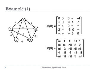
Example (1)

0 3 8 ∞ -4
2
3 4 ∞ 0 ∞ 1 7
7
8
D(0) = ∞ 4 0 ∞ ∞
1 3 2 ∞ -5 0 ∞
-4 2
1 ∞ ∞ ∞ 6 0
-5
5 4
6 nil 1 1 nil 1
nil nil nil 2 2
P(0) = nil 3 nil nil nil
4 nil 4 nil nil
nil nil nil 5 nil

Proiectarea Algoritmilor 2010

Example (2)
0 3 8 ∞ -4 0 3 8 ∞ -4
∞ 0 ∞ 1 7 ∞ 0 ∞ 1 7
D= ∞ 4 0 ∞ ∞ D= ∞ 4 0 ∞ ∞
2 ∞ -5 0 ∞ 2 5 -5 0 -2
2
∞ ∞ ∞ 6 0 3 4 ∞ ∞ ∞ 6 0
7 8
1 3
D(0), P(0) D(1), P(1)
-4 1
2 -5
nil 1 1 nil 1 5
6
4 nil 1 1 nil 1
nil nil nil 2 2 nil nil nil 2 2
p = nil 3 nil nil nil p = nil 3 nil nil nil
4 nil 4 nil nil 4 1 4 nil 1
nil nil nil 5 nil nil nil nil 5 nil

Example (3)
0 3 8 ∞ -4 0 3 8 4 -4
∞ 0 ∞ 1 7 ∞ 0 ∞ 1 7
D= ∞ 4 0 ∞ ∞ D= ∞ 4 0 5 11
2 5 -5 0 -2 2 5 -5 0 -2
2
∞ ∞ ∞ 6 0 3 4 ∞ ∞ ∞ 6 0
7 8
1 3
D(1), P(1) D(2), P(2)
-4 1
2 -5
nil 1 1 nil 1 5
6
4 nil 1 1 2 1
p = nil 3 nil nil nil p = nil 3 nil 2 2
4 1 4 nil 1 4 1 4 nil 1

Example (4)
0 3 8 4 -4 0 3 8 4 -4
∞ 0 ∞ 1 7 ∞ 0 ∞ 1 7
D= ∞ 4 0 5 11 D= ∞ 4 0 5 11
2 5 -5 0 -2 2 -1 -5 0 -2
2
∞ ∞ ∞ 6 0 3 4 ∞ ∞ ∞ 6 0
7 8
1 3
D(2), P(2) D(3), P(3)
-4 1
2 -5
nil 1 1 2 1 5
6
4 nil 1 1 2 1
p = nil 3 nil 2 2 p = nil 3 nil 2 2
4 1 4 nil 1 4 3 4 nil 1

Example (5)
0 3 8 4 -4 0 3 -1 4 -4
∞ 0 ∞ 1 7 3 0 -4 1 -1
D= ∞ 4 0 5 11 D= 7 4 0 5 3
2 -1 -5 0 -2 2 -1 -5 0 -2
2
∞ ∞ ∞ 6 0 3 4 8 5 1 6 0
7 8
1 3
D(3), P(3) D(4), P(4)
-4 1
2 -5
nil 1 1 2 1 5 4 nil 1 4 2 1
6
nil nil nil 2 2 4 nil 4 2 1
p = nil 3 nil 2 2 p= 4 3 nil 2 1
4 3 4 nil 1 4 3 4 nil 1
nil nil nil 5 nil 4 3 4 5 nil

Example (6)
0 3 -1 4 -4 0 1 -3 2 -4
3 0 -4 1 -1 3 0 -4 1 -1
D= 7 4 0 5 3 D= 7 4 0 5 3
2 -1 -5 0 -2 2 -1 -5 0 -2
2
8 5 1 6 0 3 4 8 5 1 6 0
7 8
D(4), P(4) 1 3 D(5), P(5)
-4 1
2 -5
nil 1 4 2 1 5 4 nil 3 4 5 1
6
4 nil 4 2 1 4 nil 4 2 1
p= 4 3 nil 2 1 p= 4 3 nil 2 1
4 3 4 nil 1 4 3 4 nil 1
4 3 4 5 nil 4 3 4 5 nil

Johnson’s Algorithm
 We want to find an algorithm that works better than
F-W for sparse graphs
 Use SSSP algorithms
 No negative edges: use Dijkstra – n times  (n2*logn)
 Problem if we have negative weight edges  cannot use
Dijkstra  B-F – n times is not good enough  (n3)
 Therefore, we want to find an (n2*logn) algorithm
that works on both positive and negative weight
edges!

 Combines Bellman-Ford and Dijkstra

Johnson’s Algorithm – Idea
 We would like:
 To transform any negative-weighted graph into a graph
with positive weights
 Such that the minimum path using the new weights is the
same path for the original weights

 (G, W) => (G, W1)
 w(u, v) can be negative
 w1(u, v) >= 0 for all (u, v)
 p is a minimum path u..v in (G, W) => p is also a minimum
path u..v in (G, W1)

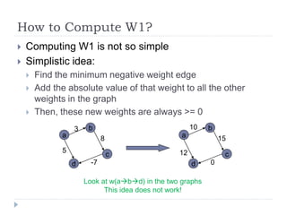
How to Compute W1?
 Computing W1 is not so simple
 Simplistic idea:
 Find the minimum negative weight edge
 Add the absolute value of that weight to all the other
weights in the graph
 Then, these new weights are always >= 0
3 b 10 b
a 8 a 15
5 12
c c
d -7 d 0

Look at w(abd) in the two graphs
This idea does not work!

How to Compute W1? Use B-F
 New idea: build a new graph G’(V’, E’)
 V’ = V U {s}
 E’ = E U {(s, v) for all vV}
 w’(s, v) = 0 for all vV
 w’(u, v) = w(u, v) for all u,vV
 Run Bellman-Ford on G’ from s
 The result is h(v)= δ(s, v) in G’ for all vV
 h(v) may be positive or negative
 We can also detect the negative cycles in G’
 The new weight function for G is:
 w1(u, v) = w(u, v) + h(u) – h(v) >= 0 for all (u, v)E

Properties of G’ and W1
 For any path p = <v0, v1, …, vk> in G:
 w1(p) = w(p) + h(v0) – h(vk)

 The negative weight cycles in G’ are the same as the
negative weight cycles in G. Why?
 Because the weight of all the cycles is the same for w1 as for w
 Cycle p => v0 = vk => w1(p) = w(p)

 Prove that w1(u, v) = w(u, v) + h(u) – h(v) >= 0 for all (u,
v)E
 Use triangle inequality for edge (u, v)E
 In G’, we have h(v) = δ(s, v) <= h(u) + w(u, v) = δ(s, u) + w(u, v)
 Therefore h(u) + w(u, v) – h(v) >= 0

Johnson’s Algorithm – Pseudocode
JOHNSON(G, W)
G’ = (V’,E’);
V’ = V  {s}; // add new source s
E’ = E  (s,u), uV; w’(s,u) = 0;
IF (BF(G’, W’) == FALSE) // run BF on G’
PRINT “Error! Negative cycle was found!”
ELSE
FOREACH (vV)
h(v) = δ(s,v); // computed by Bellman Ford
FOREACH ((u,v)E)
w1(u,v) = w(u,v) + h(u) - h(v) // compute new positive weights
FOREACH (uV)
Dijkstra(G,w1,u) // run Dijkstra for each vertex as a source using w1
FOREACH (vV)
d(u,v) = δ1(u,v) + h(v) - h(u) // we need to switch back from w1 to w

Time complexity: (n*m + n2*logn)  (n2 * logn) for sparse graphs

Example (1)

0 -1
2 0 2
3 4 3 4
7 0 0 7
0 8 -5
8 s 1 3
1 3
1 1
2 0 -4 2
-4 -5 -5
5 4 5 4
6 0 6 0
Add s and run -4
B-F on the
new graph.


Example (2)
0 -1
0 2
3 4
0 0 7
0 8 -5
s 1 3
5 -1
1
0 -4 2 1
-5 2
5 4 4 0
0 6 0 0 0 10
-4 0 13 -5
s 1 3
0
4 0 2
0

w1(u,v) = w(u,v) + h(u) - h(v) 5 4
0 2 0
-4


Example (3)
5 -1
2/1
1 2
2
4 0
0 0 4 0
10 -5 0/0 2/-3
0 13 10
s 1 3 13
1 3
0
4 0 2 0
0 0 2
0
5 4
0 2 0 5 4
-4 2
0/-4 2/2
Remove s

Run Dijkstra from each vertex => (δ1(u, v)).
Recompute the distances:
d(u,v) = δ1(u,v) + h(v) - h(u)


Example (4)
0/0 0/4
2 2
4 0 4 0
2/3 10 0/-4 2/7 10 0/0
13 13
1 3 1 3
0 2 0
0
2
0
0 1 -3 2 -4 0 0
5 4 3 0 -4 1 -1 5 4
2 2
2/-1 0/1 7 4 0 5 3 2/3 0/5
0/-1 2 -1 -5 0 -2 2/5
2 2
4 0 8 5 1 6 0 4 0
2/2 10 0/-5 4/8 10 2/1
13 13
1 3 1 3
2 0 2 0
0 0 0 0
5 4 5 4
2 2
2/-2 0/0 0/0 2/6

Application: Transitive Closure
 Given a graph G(V, E)
 Compute the transitive closure of G: G*(V, E*)
 E* = {(u, v) | there exists at least a path in G from u
to v, u..v}
 G* is an unweighted graph  we only need to
compute E* or the adjacency matrix of G*

 We can use different algorithms
 One algorithm is an adapted version of Floyd-
Warshall
 Initialize A(0)[i, j] = 1 if (i, j)E and A(0)[i, j] = 0 o/w
 A(k)[i, j] = A(k-1)[i, j] OR (A(k-1)[i, k] AND A(k-1)[k, j])

Transitive Closure – Pseudocode
TRANSITIVE-CLOSURE(G, W)
n = |V[G]|
FOR (i = 1; i <= n; i++)
FOR (j = 1; j <= n; j++)
IF (W[i][j] != INF)
A[0][i][j] = 1
ELSE
A[0][i][j] = 0
FOR (k = 1; k <= n; k++)
FOR (i = 1; i <= n; i++)
FOR (j = 1; j <= n; j++)
A[k][i][j] = A[k-1][i][j] OR (A[k-1][i][k] AND A[k-1][k][j])
RETURN A[n]

Conclusions
 We can use SSSP algorithms for computing APSP

 But there are better solutions specific to the APSP
problem!

 Floyd-Warshall for dense graphs: (n3)
 Johnson for sparse graphs: (n2 * logn)

References
 CLRS – Chapter 25

 R. Sedgewick, K Wayne – Algorithms and Data
Structures – Princeton 2007
www.cs.princeton.edu/~rs/AlgsDS07/
 Problem 1 and the corresponding images are taken from these
slides!

 MIT OCW – Introduction to Algorithms – video lecture 19

Algorithm Design and Complexity - Course 11

More Related Content

What's hot (20)

Similar to Algorithm Design and Complexity - Course 11 (20)

More from Traian Rebedea (20)

Recently uploaded (20)

Algorithm Design and Complexity - Course 11