algorithm_6dynamic_programming.pdf
0 likes78 views

The document outlines the principles of dynamic programming, emphasizing its application in optimization problems, including weighted interval scheduling, maze routing, and the traveling salesman problem. It discusses the methodology involving recursion and memoization to break down problems into manageable subproblems while also contrasting it with divide-and-conquer approaches. The document provides examples and emphasizes the importance of efficiently handling recursive calls to optimize performance.


![IRIS H.-R. JIANG
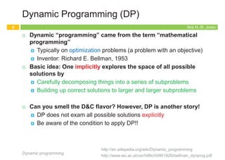
Designing a Recursive Algorithm (2/3)
¨ Second attempt: Induction on interval index
¤ First of all, sort intervals in ascending order of finish times
¤ In fact, this is also a trick for DP
¨ p(j) is the largest index i < j s.t. intervals i and j are disjoint
¤ p(j) = 0 if no request i < j is disjoint from j
Dynamic programming
9
1
2
2
4
4
7
p(1) = 0
p(2) = 0
p(3) = 1
p(4) = 0
p(5) = 3
p(6) = 3
1
2
3
4
5
6
p(2) = 0
p(6) = 3
4
1
4
IRIS H.-R. JIANG
Designing a Recursive Algorithm (3/3)
¨ Oj = the optimal solution for intervals 1, …, j
¨ OPT(j) = the value of the optimal solution for intervals 1, …, j
¤ e.g., O6 = ? Include interval 6 or not?
n Þ O6 = {6, O3} or O5
n OPT(6) = max{{v6+OPT(3)}, OPT(5)}
¤ OPT(j) = max{{vj+OPT(p(j))}, OPT(j-1)}
Dynamic programming
10
1
2
2
4
4
7
p(1) = 0
p(2) = 0
p(3) = 1
p(4) = 0
p(5) = 3
p(6) = 3
1
2
3
4
5
6 1
IRIS H.-R. JIANG
Direct Implementation
Dynamic programming
11
// Preprocessing:
// 1. Sort intervals by finish times: f1 £ f2 £ ... £ fn
// 2. Compute p(1), p(2), …, p(n)
Compute-Opt(j)
1. if (j = 0) then return 0
2. else return max{{vj+Compute-Opt(p(j))}, Compute-Opt(j-1)}
OPT(j) = max{{vj+OPT(p(j))}, OPT(j-1)}
5
4
3
1
2
1
3
2 1
1
6
3
2 1
1
The tree of calls widens very quickly
due to recursive branching!
1
2
2
4
4
7
p(1) = 0
p(2) = 0
p(3) = 1
p(4) = 0
p(5) = 3
p(6) = 3
IRIS H.-R. JIANG
Memoization: Top-Down
¨ The tree of calls widens very quickly due to recursive
branching!
¤ e.g., exponential running time when p(j) = j – 2 for all j
¨ Q: What’s wrong? A: Redundant calls!
¨ Q: How to eliminate this redundancy?
¨ A: Store the value for future! (memoization)
Dynamic programming
12
5
4
3
1
2
1
3
2 1
1
6
3
2 1
1
3
1
2
1
3
2 1
1
3
2 1
1
M-Compute-Opt(j)
1. if (j = 0) then return 0
2. else if (M[j] is not empty) then return M[j]
3. else return M[j] = max{{vj+M-Compute-Opt(p(j))},
M-Compute-Opt(j-1)}
Running time:
O(n)
How to report the
optimal solution O?
5
4
3
2
1
6](https://image.slidesharecdn.com/algorithm6dynamicprogramming-220522073057-711c84d9/85/algorithm_6dynamic_programming-pdf-9-320.jpg)
![IRIS H.-R. JIANG
Designing a Recursive Algorithm (2/3)
¨ Second attempt: Induction on interval index
¤ First of all, sort intervals in ascending order of finish times
¤ In fact, this is also a trick for DP
¨ p(j) is the largest index i < j s.t. intervals i and j are disjoint
¤ p(j) = 0 if no request i < j is disjoint from j
Dynamic programming
9
1
2
2
4
4
7
p(1) = 0
p(2) = 0
p(3) = 1
p(4) = 0
p(5) = 3
p(6) = 3
1
2
3
4
5
6
p(2) = 0
p(6) = 3
4
1
4
IRIS H.-R. JIANG
Designing a Recursive Algorithm (3/3)
¨ Oj = the optimal solution for intervals 1, …, j
¨ OPT(j) = the value of the optimal solution for intervals 1, …, j
¤ e.g., O6 = ? Include interval 6 or not?
n Þ O6 = {6, O3} or O5
n OPT(6) = max{{v6+OPT(3)}, OPT(5)}
¤ OPT(j) = max{{vj+OPT(p(j))}, OPT(j-1)}
Dynamic programming
10
1
2
2
4
4
7
p(1) = 0
p(2) = 0
p(3) = 1
p(4) = 0
p(5) = 3
p(6) = 3
1
2
3
4
5
6 1
IRIS H.-R. JIANG
Direct Implementation
Dynamic programming
11
// Preprocessing:
// 1. Sort intervals by finish times: f1 £ f2 £ ... £ fn
// 2. Compute p(1), p(2), …, p(n)
Compute-Opt(j)
1. if (j = 0) then return 0
2. else return max{{vj+Compute-Opt(p(j))}, Compute-Opt(j-1)}
OPT(j) = max{{vj+OPT(p(j))}, OPT(j-1)}
5
4
3
1
2
1
3
2 1
1
6
3
2 1
1
The tree of calls widens very quickly
due to recursive branching!
1
2
2
4
4
7
p(1) = 0
p(2) = 0
p(3) = 1
p(4) = 0
p(5) = 3
p(6) = 3
IRIS H.-R. JIANG
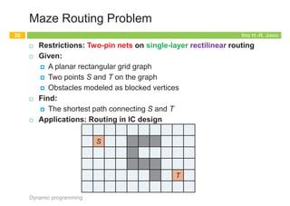
Memoization: Top-Down
¨ The tree of calls widens very quickly due to recursive
branching!
¤ e.g., exponential running time when p(j) = j – 2 for all j
¨ Q: What’s wrong? A: Redundant calls!
¨ Q: How to eliminate this redundancy?
¨ A: Store the value for future! (memoization)
Dynamic programming
12
5
4
3
1
2
1
3
2 1
1
6
3
2 1
1
3
1
2
1
3
2 1
1
3
2 1
1
M-Compute-Opt(j)
1. if (j = 0) then return 0
2. else if (M[j] is not empty) then return M[j]
3. else return M[j] = max{{vj+M-Compute-Opt(p(j))},
M-Compute-Opt(j-1)}
Running time:
O(n)
How to report the
optimal solution O?
5
4
3
2
1
6](https://image.slidesharecdn.com/algorithm6dynamicprogramming-220522073057-711c84d9/85/algorithm_6dynamic_programming-pdf-10-320.jpg)
![IRIS H.-R. JIANG
Designing a Recursive Algorithm (2/3)
¨ Second attempt: Induction on interval index
¤ First of all, sort intervals in ascending order of finish times
¤ In fact, this is also a trick for DP
¨ p(j) is the largest index i < j s.t. intervals i and j are disjoint
¤ p(j) = 0 if no request i < j is disjoint from j
Dynamic programming
9
1
2
2
4
4
7
p(1) = 0
p(2) = 0
p(3) = 1
p(4) = 0
p(5) = 3
p(6) = 3
1
2
3
4
5
6
p(2) = 0
p(6) = 3
4
1
4
IRIS H.-R. JIANG
Designing a Recursive Algorithm (3/3)
¨ Oj = the optimal solution for intervals 1, …, j
¨ OPT(j) = the value of the optimal solution for intervals 1, …, j
¤ e.g., O6 = ? Include interval 6 or not?
n Þ O6 = {6, O3} or O5
n OPT(6) = max{{v6+OPT(3)}, OPT(5)}
¤ OPT(j) = max{{vj+OPT(p(j))}, OPT(j-1)}
Dynamic programming
10
1
2
2
4
4
7
p(1) = 0
p(2) = 0
p(3) = 1
p(4) = 0
p(5) = 3
p(6) = 3
1
2
3
4
5
6 1
IRIS H.-R. JIANG
Direct Implementation
Dynamic programming
11
// Preprocessing:
// 1. Sort intervals by finish times: f1 £ f2 £ ... £ fn
// 2. Compute p(1), p(2), …, p(n)
Compute-Opt(j)
1. if (j = 0) then return 0
2. else return max{{vj+Compute-Opt(p(j))}, Compute-Opt(j-1)}
OPT(j) = max{{vj+OPT(p(j))}, OPT(j-1)}
5
4
3
1
2
1
3
2 1
1
6
3
2 1
1
The tree of calls widens very quickly
due to recursive branching!
1
2
2
4
4
7
p(1) = 0
p(2) = 0
p(3) = 1
p(4) = 0
p(5) = 3
p(6) = 3
IRIS H.-R. JIANG
Memoization: Top-Down
¨ The tree of calls widens very quickly due to recursive
branching!
¤ e.g., exponential running time when p(j) = j – 2 for all j
¨ Q: What’s wrong? A: Redundant calls!
¨ Q: How to eliminate this redundancy?
¨ A: Store the value for future! (memoization)
Dynamic programming
12
5
4
3
1
2
1
3
2 1
1
6
3
2 1
1
3
1
2
1
3
2 1
1
3
2 1
1
M-Compute-Opt(j)
1. if (j = 0) then return 0
2. else if (M[j] is not empty) then return M[j]
3. else return M[j] = max{{vj+M-Compute-Opt(p(j))},
M-Compute-Opt(j-1)}
Running time:
O(n)
How to report the
optimal solution O?
5
4
3
2
1
6](https://image.slidesharecdn.com/algorithm6dynamicprogramming-220522073057-711c84d9/85/algorithm_6dynamic_programming-pdf-11-320.jpg)
![IRIS H.-R. JIANG
Designing a Recursive Algorithm (2/3)
¨ Second attempt: Induction on interval index
¤ First of all, sort intervals in ascending order of finish times
¤ In fact, this is also a trick for DP
¨ p(j) is the largest index i < j s.t. intervals i and j are disjoint
¤ p(j) = 0 if no request i < j is disjoint from j
Dynamic programming
9
1
2
2
4
4
7
p(1) = 0
p(2) = 0
p(3) = 1
p(4) = 0
p(5) = 3
p(6) = 3
1
2
3
4
5
6
p(2) = 0
p(6) = 3
4
1
4
IRIS H.-R. JIANG
Designing a Recursive Algorithm (3/3)
¨ Oj = the optimal solution for intervals 1, …, j
¨ OPT(j) = the value of the optimal solution for intervals 1, …, j
¤ e.g., O6 = ? Include interval 6 or not?
n Þ O6 = {6, O3} or O5
n OPT(6) = max{{v6+OPT(3)}, OPT(5)}
¤ OPT(j) = max{{vj+OPT(p(j))}, OPT(j-1)}
Dynamic programming
10
1
2
2
4
4
7
p(1) = 0
p(2) = 0
p(3) = 1
p(4) = 0
p(5) = 3
p(6) = 3
1
2
3
4
5
6 1
IRIS H.-R. JIANG
Direct Implementation
Dynamic programming
11
// Preprocessing:
// 1. Sort intervals by finish times: f1 £ f2 £ ... £ fn
// 2. Compute p(1), p(2), …, p(n)
Compute-Opt(j)
1. if (j = 0) then return 0
2. else return max{{vj+Compute-Opt(p(j))}, Compute-Opt(j-1)}
OPT(j) = max{{vj+OPT(p(j))}, OPT(j-1)}
5
4
3
1
2
1
3
2 1
1
6
3
2 1
1
The tree of calls widens very quickly
due to recursive branching!
1
2
2
4
4
7
p(1) = 0
p(2) = 0
p(3) = 1
p(4) = 0
p(5) = 3
p(6) = 3
IRIS H.-R. JIANG
Memoization: Top-Down
¨ The tree of calls widens very quickly due to recursive
branching!
¤ e.g., exponential running time when p(j) = j – 2 for all j
¨ Q: What’s wrong? A: Redundant calls!
¨ Q: How to eliminate this redundancy?
¨ A: Store the value for future! (memoization)
Dynamic programming
12
5
4
3
1
2
1
3
2 1
1
6
3
2 1
1
3
1
2
1
3
2 1
1
3
2 1
1
M-Compute-Opt(j)
1. if (j = 0) then return 0
2. else if (M[j] is not empty) then return M[j]
3. else return M[j] = max{{vj+M-Compute-Opt(p(j))},
M-Compute-Opt(j-1)}
Running time:
O(n)
How to report the
optimal solution O?
5
4
3
2
1
6](https://image.slidesharecdn.com/algorithm6dynamicprogramming-220522073057-711c84d9/85/algorithm_6dynamic_programming-pdf-12-320.jpg)
![IRIS H.-R. JIANG
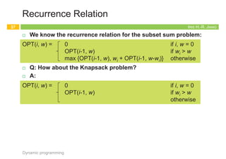
Iteration: Bottom-Up
¨ We can also compute the array M[j] by an iterative algorithm.
Dynamic programming
13
I-Compute-Opt
1. M[0] = 0
2. for j = 1, 2, .., n do
3. M[j] = max{vj+M[p(j)], M[j-1]}
Running time:
O(n)
1
2
2
4
4
7
p(1) = 0
p(2) = 0
p(3) = 1
p(4) = 0
p(5) = 3
p(6) = 3
1
2
3
4
5
6
0 2 4
0 2 4 6
0 2 4 6 7
0 2 4 6 7 8
0 2 4 6 7 8 8
M =
0 1 2 3 4 5
0
6
0 2
max{4+0, 2}
IRIS H.-R. JIANG
Summary: Memoization vs. Iteration
¨ Top-down
¨ An recursive algorithm
¤ Compute only what we need
¨ Bottom-up
¨ An iterative algorithm
¤ Construct solutions from the
smallest subproblem to the
largest one
¤ Compute every small piece
Memoization Iteration
14
Dynamic programming
The running time and
memory requirement highly
depend on the table size
Start with the recursive
divide-and-conquer
algorithm
IRIS H.-R. JIANG
Keys for Dynamic Programming
¨ Dynamic programming can be used if the problem satisfies the
following properties:
¤ There are only a polynomial number of subproblems
¤ The solution to the original problem can be easily computed from
the solutions to the subproblems
¤ There is a natural ordering on subproblems from “smallest” to
“largest,” together with an easy-to-compute recurrence
Dynamic programming
15
5
4
3
1
2
1
3
2 1
1
6
3
2 1
1
3
1
2
1
3
2 1
1
3
2 1
1
5
4
3
2
1
6
IRIS H.-R. JIANG
Keys for Dynamic Programming
¨ DP typically is applied to optimization problems.
¨ DP works best on objects that are linearly ordered an cannot be
rearranged
¨ Elements of DP
¤ Optimal substructure: an optimal solution contains within its
optimal solutions to subproblems.
¤ Overlapping subproblem: a recursive algorithm revisits the same
problem over and over again; typically, the total number of distinct
subproblems is a polynomial in the input size.
Dynamic programming
16
Cormen, Leiserson, Rivest, Stein, Introduction to Algorithms,
2nd Ed., McGraw Hill/MIT Press, 2001
5
4
3
1
2
1
3
2 1
1
6
3
2 1
1
3
1
2
1
3
2 1
1
3
2 1
1
5
4
3
2
1
6
In optimization problems, we
are interested in finding a thing
which maximizes or minimizes
some function.](https://image.slidesharecdn.com/algorithm6dynamicprogramming-220522073057-711c84d9/85/algorithm_6dynamic_programming-pdf-13-320.jpg)
![IRIS H.-R. JIANG
Iteration: Bottom-Up
¨ We can also compute the array M[j] by an iterative algorithm.
Dynamic programming
13
I-Compute-Opt
1. M[0] = 0
2. for j = 1, 2, .., n do
3. M[j] = max{vj+M[p(j)], M[j-1]}
Running time:
O(n)
1
2
2
4
4
7
p(1) = 0
p(2) = 0
p(3) = 1
p(4) = 0
p(5) = 3
p(6) = 3
1
2
3
4
5
6
0 2 4
0 2 4 6
0 2 4 6 7
0 2 4 6 7 8
0 2 4 6 7 8 8
M =
0 1 2 3 4 5
0
6
0 2
max{4+0, 2}
IRIS H.-R. JIANG
Summary: Memoization vs. Iteration
¨ Top-down
¨ An recursive algorithm
¤ Compute only what we need
¨ Bottom-up
¨ An iterative algorithm
¤ Construct solutions from the
smallest subproblem to the
largest one
¤ Compute every small piece
Memoization Iteration
14
Dynamic programming
The running time and
memory requirement highly
depend on the table size
Start with the recursive
divide-and-conquer
algorithm
IRIS H.-R. JIANG
Keys for Dynamic Programming
¨ Dynamic programming can be used if the problem satisfies the
following properties:
¤ There are only a polynomial number of subproblems
¤ The solution to the original problem can be easily computed from
the solutions to the subproblems
¤ There is a natural ordering on subproblems from “smallest” to
“largest,” together with an easy-to-compute recurrence
Dynamic programming
15
5
4
3
1
2
1
3
2 1
1
6
3
2 1
1
3
1
2
1
3
2 1
1
3
2 1
1
5
4
3
2
1
6
IRIS H.-R. JIANG
Keys for Dynamic Programming
¨ DP typically is applied to optimization problems.
¨ DP works best on objects that are linearly ordered an cannot be
rearranged
¨ Elements of DP
¤ Optimal substructure: an optimal solution contains within its
optimal solutions to subproblems.
¤ Overlapping subproblem: a recursive algorithm revisits the same
problem over and over again; typically, the total number of distinct
subproblems is a polynomial in the input size.
Dynamic programming
16
Cormen, Leiserson, Rivest, Stein, Introduction to Algorithms,
2nd Ed., McGraw Hill/MIT Press, 2001
5
4
3
1
2
1
3
2 1
1
6
3
2 1
1
3
1
2
1
3
2 1
1
3
2 1
1
5
4
3
2
1
6
In optimization problems, we
are interested in finding a thing
which maximizes or minimizes
some function.](https://image.slidesharecdn.com/algorithm6dynamicprogramming-220522073057-711c84d9/85/algorithm_6dynamic_programming-pdf-14-320.jpg)
![IRIS H.-R. JIANG
Iteration: Bottom-Up
¨ We can also compute the array M[j] by an iterative algorithm.
Dynamic programming
13
I-Compute-Opt
1. M[0] = 0
2. for j = 1, 2, .., n do
3. M[j] = max{vj+M[p(j)], M[j-1]}
Running time:
O(n)
1
2
2
4
4
7
p(1) = 0
p(2) = 0
p(3) = 1
p(4) = 0
p(5) = 3
p(6) = 3
1
2
3
4
5
6
0 2 4
0 2 4 6
0 2 4 6 7
0 2 4 6 7 8
0 2 4 6 7 8 8
M =
0 1 2 3 4 5
0
6
0 2
max{4+0, 2}
IRIS H.-R. JIANG
Summary: Memoization vs. Iteration
¨ Top-down
¨ An recursive algorithm
¤ Compute only what we need
¨ Bottom-up
¨ An iterative algorithm
¤ Construct solutions from the
smallest subproblem to the
largest one
¤ Compute every small piece
Memoization Iteration
14
Dynamic programming
The running time and
memory requirement highly
depend on the table size
Start with the recursive
divide-and-conquer
algorithm
IRIS H.-R. JIANG
Keys for Dynamic Programming
¨ Dynamic programming can be used if the problem satisfies the
following properties:
¤ There are only a polynomial number of subproblems
¤ The solution to the original problem can be easily computed from
the solutions to the subproblems
¤ There is a natural ordering on subproblems from “smallest” to
“largest,” together with an easy-to-compute recurrence
Dynamic programming
15
5
4
3
1
2
1
3
2 1
1
6
3
2 1
1
3
1
2
1
3
2 1
1
3
2 1
1
5
4
3
2
1
6
IRIS H.-R. JIANG
Keys for Dynamic Programming
¨ DP typically is applied to optimization problems.
¨ DP works best on objects that are linearly ordered an cannot be
rearranged
¨ Elements of DP
¤ Optimal substructure: an optimal solution contains within its
optimal solutions to subproblems.
¤ Overlapping subproblem: a recursive algorithm revisits the same
problem over and over again; typically, the total number of distinct
subproblems is a polynomial in the input size.
Dynamic programming
16
Cormen, Leiserson, Rivest, Stein, Introduction to Algorithms,
2nd Ed., McGraw Hill/MIT Press, 2001
5
4
3
1
2
1
3
2 1
1
6
3
2 1
1
3
1
2
1
3
2 1
1
3
2 1
1
5
4
3
2
1
6
In optimization problems, we
are interested in finding a thing
which maximizes or minimizes
some function.](https://image.slidesharecdn.com/algorithm6dynamicprogramming-220522073057-711c84d9/85/algorithm_6dynamic_programming-pdf-15-320.jpg)
![IRIS H.-R. JIANG
Iteration: Bottom-Up
¨ We can also compute the array M[j] by an iterative algorithm.
Dynamic programming
13
I-Compute-Opt
1. M[0] = 0
2. for j = 1, 2, .., n do
3. M[j] = max{vj+M[p(j)], M[j-1]}
Running time:
O(n)
1
2
2
4
4
7
p(1) = 0
p(2) = 0
p(3) = 1
p(4) = 0
p(5) = 3
p(6) = 3
1
2
3
4
5
6
0 2 4
0 2 4 6
0 2 4 6 7
0 2 4 6 7 8
0 2 4 6 7 8 8
M =
0 1 2 3 4 5
0
6
0 2
max{4+0, 2}
IRIS H.-R. JIANG
Summary: Memoization vs. Iteration
¨ Top-down
¨ An recursive algorithm
¤ Compute only what we need
¨ Bottom-up
¨ An iterative algorithm
¤ Construct solutions from the
smallest subproblem to the
largest one
¤ Compute every small piece
Memoization Iteration
14
Dynamic programming
The running time and
memory requirement highly
depend on the table size
Start with the recursive
divide-and-conquer
algorithm
IRIS H.-R. JIANG
Keys for Dynamic Programming
¨ Dynamic programming can be used if the problem satisfies the
following properties:
¤ There are only a polynomial number of subproblems
¤ The solution to the original problem can be easily computed from
the solutions to the subproblems
¤ There is a natural ordering on subproblems from “smallest” to
“largest,” together with an easy-to-compute recurrence
Dynamic programming
15
5
4
3
1
2
1
3
2 1
1
6
3
2 1
1
3
1
2
1
3
2 1
1
3
2 1
1
5
4
3
2
1
6
IRIS H.-R. JIANG
Keys for Dynamic Programming
¨ DP typically is applied to optimization problems.
¨ DP works best on objects that are linearly ordered an cannot be
rearranged
¨ Elements of DP
¤ Optimal substructure: an optimal solution contains within its
optimal solutions to subproblems.
¤ Overlapping subproblem: a recursive algorithm revisits the same
problem over and over again; typically, the total number of distinct
subproblems is a polynomial in the input size.
Dynamic programming
16
Cormen, Leiserson, Rivest, Stein, Introduction to Algorithms,
2nd Ed., McGraw Hill/MIT Press, 2001
5
4
3
1
2
1
3
2 1
1
6
3
2 1
1
3
1
2
1
3
2 1
1
3
2 1
1
5
4
3
2
1
6
In optimization problems, we
are interested in finding a thing
which maximizes or minimizes
some function.](https://image.slidesharecdn.com/algorithm6dynamicprogramming-220522073057-711c84d9/85/algorithm_6dynamic_programming-pdf-16-320.jpg)


![IRIS H.-R. JIANG
What’s Wrong?
¨ What if we call fib(5)?
¤ fib(5)
¤ fib(4) + fib(3)
¤ (fib(3) + fib(2)) + (fib(2) + fib(1))
¤ ((fib(2) + fib(1)) + (fib(1) + fib(0))) + ((fib(1) + fib(0)) + fib(1))
¤ (((fib(1) + fib(0)) + fib(1))+(fib(1) + fib(0)))+((fib(1) + fib(0))+fib(1))
¤ A call tree that calls the function on the same value many
different times
n fib(2) was calculated three times from scratch
n Impractical for large n
Dynamic programming
21
fib(n)
1. if n £ 1 return n
2. return fib(n ! 1) + fib(n ! 2)
5
4
3
2
3
2 1
2
1 0 1 0
1
1 0
2
1 0
2
1 0
2
1 0
IRIS H.-R. JIANG
Too Many Redundant Calls!
¨ How to remove redundancy?
¤ Prevent repeated calculation
Recursion True dependency
Dynamic programming
22
5
4 3
2 1
5
4
3
2
3
2 1
2
1 0 1 0
1
1 0
3
2
3
1
2
1 0
1
1 0
2
1 0
2
1 0
2
1 0
IRIS H.-R. JIANG
Dynamic Programming -- Memoization
¨ Store the values in a table
¤ Check the table before a recursive call
¤ Top-down!
n The control flow is almost the same as the original one
Dynamic programming
23
fib(n)
1. Initialize f[0..n] with -1 // -1: unfilled
2. f[0] = 0; f[1] = 1
3. fibonacci(n, f)
fibonacci(n, f)
1. If f[n] == -1 then
2. f[n] = fibonacci(n ! 1, f) + fibonacci(n ! 2, f)
3. return f[n] // if f[n] already exists, directly return
5
4 3
2 1
IRIS H.-R. JIANG
Dynamic Programming -- Bottom-up?
¨ Store the values in a table
¤ Bottom-up
n Compute the values for small problems first
¤ Much like induction
Dynamic programming
24
fib(n)
1. initialize f[1..n] with -1 // -1: unfilled
2. f[0] = 0; f[1] = 1
3. for i=2 to n do
4. f[i] = f[i-1]+ f[i-2]
5. return f[n]
5
4 3
2 1](https://image.slidesharecdn.com/algorithm6dynamicprogramming-220522073057-711c84d9/85/algorithm_6dynamic_programming-pdf-21-320.jpg)
![IRIS H.-R. JIANG
What’s Wrong?
¨ What if we call fib(5)?
¤ fib(5)
¤ fib(4) + fib(3)
¤ (fib(3) + fib(2)) + (fib(2) + fib(1))
¤ ((fib(2) + fib(1)) + (fib(1) + fib(0))) + ((fib(1) + fib(0)) + fib(1))
¤ (((fib(1) + fib(0)) + fib(1))+(fib(1) + fib(0)))+((fib(1) + fib(0))+fib(1))
¤ A call tree that calls the function on the same value many
different times
n fib(2) was calculated three times from scratch
n Impractical for large n
Dynamic programming
21
fib(n)
1. if n £ 1 return n
2. return fib(n ! 1) + fib(n ! 2)
5
4
3
2
3
2 1
2
1 0 1 0
1
1 0
2
1 0
2
1 0
2
1 0
IRIS H.-R. JIANG
Too Many Redundant Calls!
¨ How to remove redundancy?
¤ Prevent repeated calculation
Recursion True dependency
Dynamic programming
22
5
4 3
2 1
5
4
3
2
3
2 1
2
1 0 1 0
1
1 0
3
2
3
1
2
1 0
1
1 0
2
1 0
2
1 0
2
1 0
IRIS H.-R. JIANG
Dynamic Programming -- Memoization
¨ Store the values in a table
¤ Check the table before a recursive call
¤ Top-down!
n The control flow is almost the same as the original one
Dynamic programming
23
fib(n)
1. Initialize f[0..n] with -1 // -1: unfilled
2. f[0] = 0; f[1] = 1
3. fibonacci(n, f)
fibonacci(n, f)
1. If f[n] == -1 then
2. f[n] = fibonacci(n ! 1, f) + fibonacci(n ! 2, f)
3. return f[n] // if f[n] already exists, directly return
5
4 3
2 1
IRIS H.-R. JIANG
Dynamic Programming -- Bottom-up?
¨ Store the values in a table
¤ Bottom-up
n Compute the values for small problems first
¤ Much like induction
Dynamic programming
24
fib(n)
1. initialize f[1..n] with -1 // -1: unfilled
2. f[0] = 0; f[1] = 1
3. for i=2 to n do
4. f[i] = f[i-1]+ f[i-2]
5. return f[n]
5
4 3
2 1](https://image.slidesharecdn.com/algorithm6dynamicprogramming-220522073057-711c84d9/85/algorithm_6dynamic_programming-pdf-22-320.jpg)
![IRIS H.-R. JIANG
What’s Wrong?
¨ What if we call fib(5)?
¤ fib(5)
¤ fib(4) + fib(3)
¤ (fib(3) + fib(2)) + (fib(2) + fib(1))
¤ ((fib(2) + fib(1)) + (fib(1) + fib(0))) + ((fib(1) + fib(0)) + fib(1))
¤ (((fib(1) + fib(0)) + fib(1))+(fib(1) + fib(0)))+((fib(1) + fib(0))+fib(1))
¤ A call tree that calls the function on the same value many
different times
n fib(2) was calculated three times from scratch
n Impractical for large n
Dynamic programming
21
fib(n)
1. if n £ 1 return n
2. return fib(n ! 1) + fib(n ! 2)
5
4
3
2
3
2 1
2
1 0 1 0
1
1 0
2
1 0
2
1 0
2
1 0
IRIS H.-R. JIANG
Too Many Redundant Calls!
¨ How to remove redundancy?
¤ Prevent repeated calculation
Recursion True dependency
Dynamic programming
22
5
4 3
2 1
5
4
3
2
3
2 1
2
1 0 1 0
1
1 0
3
2
3
1
2
1 0
1
1 0
2
1 0
2
1 0
2
1 0
IRIS H.-R. JIANG
Dynamic Programming -- Memoization
¨ Store the values in a table
¤ Check the table before a recursive call
¤ Top-down!
n The control flow is almost the same as the original one
Dynamic programming
23
fib(n)
1. Initialize f[0..n] with -1 // -1: unfilled
2. f[0] = 0; f[1] = 1
3. fibonacci(n, f)
fibonacci(n, f)
1. If f[n] == -1 then
2. f[n] = fibonacci(n ! 1, f) + fibonacci(n ! 2, f)
3. return f[n] // if f[n] already exists, directly return
5
4 3
2 1
IRIS H.-R. JIANG
Dynamic Programming -- Bottom-up?
¨ Store the values in a table
¤ Bottom-up
n Compute the values for small problems first
¤ Much like induction
Dynamic programming
24
fib(n)
1. initialize f[1..n] with -1 // -1: unfilled
2. f[0] = 0; f[1] = 1
3. for i=2 to n do
4. f[i] = f[i-1]+ f[i-2]
5. return f[n]
5
4 3
2 1](https://image.slidesharecdn.com/algorithm6dynamicprogramming-220522073057-711c84d9/85/algorithm_6dynamic_programming-pdf-23-320.jpg)
![IRIS H.-R. JIANG
What’s Wrong?
¨ What if we call fib(5)?
¤ fib(5)
¤ fib(4) + fib(3)
¤ (fib(3) + fib(2)) + (fib(2) + fib(1))
¤ ((fib(2) + fib(1)) + (fib(1) + fib(0))) + ((fib(1) + fib(0)) + fib(1))
¤ (((fib(1) + fib(0)) + fib(1))+(fib(1) + fib(0)))+((fib(1) + fib(0))+fib(1))
¤ A call tree that calls the function on the same value many
different times
n fib(2) was calculated three times from scratch
n Impractical for large n
Dynamic programming
21
fib(n)
1. if n £ 1 return n
2. return fib(n ! 1) + fib(n ! 2)
5
4
3
2
3
2 1
2
1 0 1 0
1
1 0
2
1 0
2
1 0
2
1 0
IRIS H.-R. JIANG
Too Many Redundant Calls!
¨ How to remove redundancy?
¤ Prevent repeated calculation
Recursion True dependency
Dynamic programming
22
5
4 3
2 1
5
4
3
2
3
2 1
2
1 0 1 0
1
1 0
3
2
3
1
2
1 0
1
1 0
2
1 0
2
1 0
2
1 0
IRIS H.-R. JIANG
Dynamic Programming -- Memoization
¨ Store the values in a table
¤ Check the table before a recursive call
¤ Top-down!
n The control flow is almost the same as the original one
Dynamic programming
23
fib(n)
1. Initialize f[0..n] with -1 // -1: unfilled
2. f[0] = 0; f[1] = 1
3. fibonacci(n, f)
fibonacci(n, f)
1. If f[n] == -1 then
2. f[n] = fibonacci(n ! 1, f) + fibonacci(n ! 2, f)
3. return f[n] // if f[n] already exists, directly return
5
4 3
2 1
IRIS H.-R. JIANG
Dynamic Programming -- Bottom-up?
¨ Store the values in a table
¤ Bottom-up
n Compute the values for small problems first
¤ Much like induction
Dynamic programming
24
fib(n)
1. initialize f[1..n] with -1 // -1: unfilled
2. f[0] = 0; f[1] = 1
3. for i=2 to n do
4. f[i] = f[i-1]+ f[i-2]
5. return f[n]
5
4 3
2 1](https://image.slidesharecdn.com/algorithm6dynamicprogramming-220522073057-711c84d9/85/algorithm_6dynamic_programming-pdf-24-320.jpg)


![IRIS H.-R. JIANG
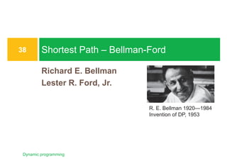
DP: Iteration
Dynamic programming
33
OPT(i, w) = 0 if i, w = 0
OPT(i-1, w) if wi > w
max {OPT(i-1, w), wi + OPT(i-1, w-wi)} otherwise
Subset-sum(n, w1,…, wn, W)
1. for w = 0, 1, …, W do
2. M[0, w] = 0
3. for i = 0, 1, …, n do
4. M[i, 0] = 0
5. for i = 1, 2, .., n do
6. for w = 1, 2, .., W do
7. if (wi > w) then
8. M[i, w] = M[i-1, w]
9. else
10. M[i, w] = max {M[i-1, w], wi +M[i-1, w-wi]}
IRIS H.-R. JIANG
Example
Dynamic programming
34
1
Weight
5
6
2
7
Item
1
3
4
5
2
W = 11
0
0
0
0
0
0 0 0 0 0 0 0 0 0 0 0 0
1 2 3 3 3 3 3 3 3 3 3
1 2 3 3 5 6 7 8 8 8 8
1 2 3 3 5 6 7 8 9 9 11
1 1 1 1 1 1 1 1 1 1 1
1 2 3 3 5 6 7 8 9 10 11
0 1 2 3 4 5 6 7 8 9 10 11
W + 1
Æ
{ 1, 2 }
{ 1, 2, 3 }
{ 1, 2, 3, 4 }
{ 1 }
{ 1, 2, 3, 4, 5 }
n + 1
Subset-sum(n, w1,…, wn, W)
1. for w = 0, 1, …, W do
2. M[0, w] = 0
3. for i = 0, 1, …, n do
4. M[i, 0] = 0
5. for i = 1, 2, .., n do
6. for w = 1, 2, .., W do
7. if (wi > w) then
8. M[i, w] = M[i-1, w]
9. else
10. M[i, w] = max{M[i-1, w], wi +M[i-1, w-wi]}
3 11
11
M
0
0
0
0
0
0 0 0 0 0 0 0 0 0 0 0 0
1 2 3 3 3 3 3 3 3 3 3
1 2 3 3 5 6 7 8 8 8 8
1 2 3 3 5 6 7 8 9 9 11
1 1 1 1 1 1 1 1 1 1 1
1 2 3 3 5 6 7 8 9 10 11
Running time:
O(nW)
IRIS H.-R. JIANG
Pseudo-Polynomial Running Time
¨ Running time: O(nW)
¤ W is not polynomial in input size
¤ “Pseudo-polynomial”
¤ In fact, the subset sum is a computationally hard problem!
n r.f. Karp's 21 NP-complete problems:
n R. M. Karp, "Reducibility among combinatorial problems".
Complexity of Computer Computations. pp. 85--103.
Dynamic programming
35
IRIS H.-R. JIANG
The Knapsack Problem
¨ Given
¤ A set of n items and a knapsack
¤ Item i weighs wi > 0 and has value vi > 0.
¤ The knapsack has capacity of W.
¨ Goal:
¤ Fill the knapsack so as to maximize total value.
n Maximize SiÎS vi
¨ Optimization problem formulation
¤ max SiÎS vi
s.t. SiÎS wi < W, SÍ{1, …, n}
¨ Greedy ¹ optimal
¤ Largest vi first: 28+6+1 = 35
¤ Optimal: 18+22 = 40
Dynamic programming
36
ue.
Karp's 21 NP-complete problems:
R. M. Karp, "Reducibility among combinatorial problems".
Complexity of Computer Computations. pp. 85–103.
1
Value
18
22
28
1
Weight
5
6
6 2
7
Item
1
3
4
5
2
W = 11](https://image.slidesharecdn.com/algorithm6dynamicprogramming-220522073057-711c84d9/85/algorithm_6dynamic_programming-pdf-33-320.jpg)
![IRIS H.-R. JIANG
DP: Iteration
Dynamic programming
33
OPT(i, w) = 0 if i, w = 0
OPT(i-1, w) if wi > w
max {OPT(i-1, w), wi + OPT(i-1, w-wi)} otherwise
Subset-sum(n, w1,…, wn, W)
1. for w = 0, 1, …, W do
2. M[0, w] = 0
3. for i = 0, 1, …, n do
4. M[i, 0] = 0
5. for i = 1, 2, .., n do
6. for w = 1, 2, .., W do
7. if (wi > w) then
8. M[i, w] = M[i-1, w]
9. else
10. M[i, w] = max {M[i-1, w], wi +M[i-1, w-wi]}
IRIS H.-R. JIANG
Example
Dynamic programming
34
1
Weight
5
6
2
7
Item
1
3
4
5
2
W = 11
0
0
0
0
0
0 0 0 0 0 0 0 0 0 0 0 0
1 2 3 3 3 3 3 3 3 3 3
1 2 3 3 5 6 7 8 8 8 8
1 2 3 3 5 6 7 8 9 9 11
1 1 1 1 1 1 1 1 1 1 1
1 2 3 3 5 6 7 8 9 10 11
0 1 2 3 4 5 6 7 8 9 10 11
W + 1
Æ
{ 1, 2 }
{ 1, 2, 3 }
{ 1, 2, 3, 4 }
{ 1 }
{ 1, 2, 3, 4, 5 }
n + 1
Subset-sum(n, w1,…, wn, W)
1. for w = 0, 1, …, W do
2. M[0, w] = 0
3. for i = 0, 1, …, n do
4. M[i, 0] = 0
5. for i = 1, 2, .., n do
6. for w = 1, 2, .., W do
7. if (wi > w) then
8. M[i, w] = M[i-1, w]
9. else
10. M[i, w] = max{M[i-1, w], wi +M[i-1, w-wi]}
3 11
11
M
0
0
0
0
0
0 0 0 0 0 0 0 0 0 0 0 0
1 2 3 3 3 3 3 3 3 3 3
1 2 3 3 5 6 7 8 8 8 8
1 2 3 3 5 6 7 8 9 9 11
1 1 1 1 1 1 1 1 1 1 1
1 2 3 3 5 6 7 8 9 10 11
Running time:
O(nW)
IRIS H.-R. JIANG
Pseudo-Polynomial Running Time
¨ Running time: O(nW)
¤ W is not polynomial in input size
¤ “Pseudo-polynomial”
¤ In fact, the subset sum is a computationally hard problem!
n r.f. Karp's 21 NP-complete problems:
n R. M. Karp, "Reducibility among combinatorial problems".
Complexity of Computer Computations. pp. 85--103.
Dynamic programming
35
IRIS H.-R. JIANG
The Knapsack Problem
¨ Given
¤ A set of n items and a knapsack
¤ Item i weighs wi > 0 and has value vi > 0.
¤ The knapsack has capacity of W.
¨ Goal:
¤ Fill the knapsack so as to maximize total value.
n Maximize SiÎS vi
¨ Optimization problem formulation
¤ max SiÎS vi
s.t. SiÎS wi < W, SÍ{1, …, n}
¨ Greedy ¹ optimal
¤ Largest vi first: 28+6+1 = 35
¤ Optimal: 18+22 = 40
Dynamic programming
36
ue.
Karp's 21 NP-complete problems:
R. M. Karp, "Reducibility among combinatorial problems".
Complexity of Computer Computations. pp. 85–103.
1
Value
18
22
28
1
Weight
5
6
6 2
7
Item
1
3
4
5
2
W = 11](https://image.slidesharecdn.com/algorithm6dynamicprogramming-220522073057-711c84d9/85/algorithm_6dynamic_programming-pdf-34-320.jpg)
![IRIS H.-R. JIANG
DP: Iteration
Dynamic programming
33
OPT(i, w) = 0 if i, w = 0
OPT(i-1, w) if wi > w
max {OPT(i-1, w), wi + OPT(i-1, w-wi)} otherwise
Subset-sum(n, w1,…, wn, W)
1. for w = 0, 1, …, W do
2. M[0, w] = 0
3. for i = 0, 1, …, n do
4. M[i, 0] = 0
5. for i = 1, 2, .., n do
6. for w = 1, 2, .., W do
7. if (wi > w) then
8. M[i, w] = M[i-1, w]
9. else
10. M[i, w] = max {M[i-1, w], wi +M[i-1, w-wi]}
IRIS H.-R. JIANG
Example
Dynamic programming
34
1
Weight
5
6
2
7
Item
1
3
4
5
2
W = 11
0
0
0
0
0
0 0 0 0 0 0 0 0 0 0 0 0
1 2 3 3 3 3 3 3 3 3 3
1 2 3 3 5 6 7 8 8 8 8
1 2 3 3 5 6 7 8 9 9 11
1 1 1 1 1 1 1 1 1 1 1
1 2 3 3 5 6 7 8 9 10 11
0 1 2 3 4 5 6 7 8 9 10 11
W + 1
Æ
{ 1, 2 }
{ 1, 2, 3 }
{ 1, 2, 3, 4 }
{ 1 }
{ 1, 2, 3, 4, 5 }
n + 1
Subset-sum(n, w1,…, wn, W)
1. for w = 0, 1, …, W do
2. M[0, w] = 0
3. for i = 0, 1, …, n do
4. M[i, 0] = 0
5. for i = 1, 2, .., n do
6. for w = 1, 2, .., W do
7. if (wi > w) then
8. M[i, w] = M[i-1, w]
9. else
10. M[i, w] = max{M[i-1, w], wi +M[i-1, w-wi]}
3 11
11
M
0
0
0
0
0
0 0 0 0 0 0 0 0 0 0 0 0
1 2 3 3 3 3 3 3 3 3 3
1 2 3 3 5 6 7 8 8 8 8
1 2 3 3 5 6 7 8 9 9 11
1 1 1 1 1 1 1 1 1 1 1
1 2 3 3 5 6 7 8 9 10 11
Running time:
O(nW)
IRIS H.-R. JIANG
Pseudo-Polynomial Running Time
¨ Running time: O(nW)
¤ W is not polynomial in input size
¤ “Pseudo-polynomial”
¤ In fact, the subset sum is a computationally hard problem!
n r.f. Karp's 21 NP-complete problems:
n R. M. Karp, "Reducibility among combinatorial problems".
Complexity of Computer Computations. pp. 85--103.
Dynamic programming
35
IRIS H.-R. JIANG
The Knapsack Problem
¨ Given
¤ A set of n items and a knapsack
¤ Item i weighs wi > 0 and has value vi > 0.
¤ The knapsack has capacity of W.
¨ Goal:
¤ Fill the knapsack so as to maximize total value.
n Maximize SiÎS vi
¨ Optimization problem formulation
¤ max SiÎS vi
s.t. SiÎS wi < W, SÍ{1, …, n}
¨ Greedy ¹ optimal
¤ Largest vi first: 28+6+1 = 35
¤ Optimal: 18+22 = 40
Dynamic programming
36
ue.
Karp's 21 NP-complete problems:
R. M. Karp, "Reducibility among combinatorial problems".
Complexity of Computer Computations. pp. 85–103.
1
Value
18
22
28
1
Weight
5
6
6 2
7
Item
1
3
4
5
2
W = 11](https://image.slidesharecdn.com/algorithm6dynamicprogramming-220522073057-711c84d9/85/algorithm_6dynamic_programming-pdf-35-320.jpg)
![IRIS H.-R. JIANG
DP: Iteration
Dynamic programming
33
OPT(i, w) = 0 if i, w = 0
OPT(i-1, w) if wi > w
max {OPT(i-1, w), wi + OPT(i-1, w-wi)} otherwise
Subset-sum(n, w1,…, wn, W)
1. for w = 0, 1, …, W do
2. M[0, w] = 0
3. for i = 0, 1, …, n do
4. M[i, 0] = 0
5. for i = 1, 2, .., n do
6. for w = 1, 2, .., W do
7. if (wi > w) then
8. M[i, w] = M[i-1, w]
9. else
10. M[i, w] = max {M[i-1, w], wi +M[i-1, w-wi]}
IRIS H.-R. JIANG
Example
Dynamic programming
34
1
Weight
5
6
2
7
Item
1
3
4
5
2
W = 11
0
0
0
0
0
0 0 0 0 0 0 0 0 0 0 0 0
1 2 3 3 3 3 3 3 3 3 3
1 2 3 3 5 6 7 8 8 8 8
1 2 3 3 5 6 7 8 9 9 11
1 1 1 1 1 1 1 1 1 1 1
1 2 3 3 5 6 7 8 9 10 11
0 1 2 3 4 5 6 7 8 9 10 11
W + 1
Æ
{ 1, 2 }
{ 1, 2, 3 }
{ 1, 2, 3, 4 }
{ 1 }
{ 1, 2, 3, 4, 5 }
n + 1
Subset-sum(n, w1,…, wn, W)
1. for w = 0, 1, …, W do
2. M[0, w] = 0
3. for i = 0, 1, …, n do
4. M[i, 0] = 0
5. for i = 1, 2, .., n do
6. for w = 1, 2, .., W do
7. if (wi > w) then
8. M[i, w] = M[i-1, w]
9. else
10. M[i, w] = max{M[i-1, w], wi +M[i-1, w-wi]}
3 11
11
M
0
0
0
0
0
0 0 0 0 0 0 0 0 0 0 0 0
1 2 3 3 3 3 3 3 3 3 3
1 2 3 3 5 6 7 8 8 8 8
1 2 3 3 5 6 7 8 9 9 11
1 1 1 1 1 1 1 1 1 1 1
1 2 3 3 5 6 7 8 9 10 11
Running time:
O(nW)
IRIS H.-R. JIANG
Pseudo-Polynomial Running Time
¨ Running time: O(nW)
¤ W is not polynomial in input size
¤ “Pseudo-polynomial”
¤ In fact, the subset sum is a computationally hard problem!
n r.f. Karp's 21 NP-complete problems:
n R. M. Karp, "Reducibility among combinatorial problems".
Complexity of Computer Computations. pp. 85--103.
Dynamic programming
35
IRIS H.-R. JIANG
The Knapsack Problem
¨ Given
¤ A set of n items and a knapsack
¤ Item i weighs wi > 0 and has value vi > 0.
¤ The knapsack has capacity of W.
¨ Goal:
¤ Fill the knapsack so as to maximize total value.
n Maximize SiÎS vi
¨ Optimization problem formulation
¤ max SiÎS vi
s.t. SiÎS wi < W, SÍ{1, …, n}
¨ Greedy ¹ optimal
¤ Largest vi first: 28+6+1 = 35
¤ Optimal: 18+22 = 40
Dynamic programming
36
ue.
Karp's 21 NP-complete problems:
R. M. Karp, "Reducibility among combinatorial problems".
Complexity of Computer Computations. pp. 85–103.
1
Value
18
22
28
1
Weight
5
6
6 2
7
Item
1
3
4
5
2
W = 11](https://image.slidesharecdn.com/algorithm6dynamicprogramming-220522073057-711c84d9/85/algorithm_6dynamic_programming-pdf-36-320.jpg)


![IRIS H.-R. JIANG
Bellman-Ford Algorithm (1/2)
¨ Induction either on nodes or on edges works!
¨ If G has no negative cycles, then there is a shortest path from s
to t that is simple (i.e., does not repeat nodes), and hence has
at most n-1 edges.
¨ Pf:
¤ Suppose the shortest path P from s to t repeat a node v.
¤ Since every cycle has nonnegative cost, we could remove the
portion of P between consecutive visits to v resulting in a simple
path Q of no greater cost and fewer edges.
n c(Q) = c(P) – c(C) £ c(P)
Dynamic programming
41
v
s t
C c(C) ³ 0
IRIS H.-R. JIANG
Bellman-Ford Algorithm (2/2)
¨ Induction on edges
¨ OPT(i, v) = length of shortest v-t path P using at most i edges.
¤ OPT(n-1, s) = length of shortest s-t path.
¤ Case 1: P uses at most i-1 edges.
n OPT(i, v) = OPT(i-1, v)
¤ Case 2: P uses exactly i edges.
n OPT(i, v) = cvw + OPT(i-1, w)
n If (v, w) is the first edge, then P uses (v, w) and then selects
the shortest w-t path using at most i-1 edges
Dynamic programming
42
v t
at most i-1 edges
:
:
w
OPT(i, v) = 0 if i = 0, v = t
¥ if i = 0, v ¹ t
min{OPT(i-1, v), min(v, w)ÎE {cvw + OPT(i-1, w)}} otherwise
t
at most i-1 edges
v
IRIS H.-R. JIANG
Implementation: Iteration
Dynamic programming
43
Bellman-Ford(G, s, t)
// n = # of nodes in G
// M[0.. n-1, V]: table recording optimal solutions of subproblems
1. M[0, t] = 0
2. foreach vÎV-{t} do
3. M[0, v] = ¥
4. for i = 1 to n-1 do
5. for vÎV in any order do
6. M[i, v]=min{M[i-1, v], min(v, w)ÎE {cvw + M[i-1, w]}}
OPT(i, v) = 0 if i = 0, v = t
¥ if i = 0, v ¹ t
min{OPT(i-1, v), min(v, w)ÎE {cvw + OPT(i-1, w)}} otherwise
IRIS H.-R. JIANG
M
Example
Dynamic programming
44
Bellman-Ford(G, s, t)
// n = # of nodes in G
// M[0.. n-1, V]: table recording optimal solutions of subproblems
1. M[0, t] = 0
2. foreach vÎV-{t} do
3. M[0, v] = ¥
4. for i = 1 to n-1 do
5. for vÎV in any order do
6. M[i, v]=min{M[i-1, v], min(v, w)ÎE {cvw + M[i-1, w]}}
¥
¥
¥
¥
¥
0
¥
3
4
-3
2
0
0
3
3
-3
0
0
-2
3
3
-4
0
0
-2
3
2
-6
0
0
-2
3
0
-6
0
0 1 2 3 4 5
n
t
b
c
d
a
e
n
0
Space: O(n2)
Running time:
1. naïve:
O(n3)
2. detailed:
O(nm)
b
d
t
e
-1
-2
4
2
c
-3
8
a
-4
6 -3
3
¥
¥
¥
¥
¥
0
¥
3
4
-3
2
0
0
3
3
-3
0
0
-2
3
3
-4
0
0
-2
3
2
-6
0
0
-2
3
0
-6
0
0
b t
e
c
a
Q: How to find the shortest path?
A: Record “successor” for each entry
M[d, 2] =min{M[d,1],
cda+M[a,1]}](https://image.slidesharecdn.com/algorithm6dynamicprogramming-220522073057-711c84d9/85/algorithm_6dynamic_programming-pdf-41-320.jpg)
![IRIS H.-R. JIANG
Bellman-Ford Algorithm (1/2)
¨ Induction either on nodes or on edges works!
¨ If G has no negative cycles, then there is a shortest path from s
to t that is simple (i.e., does not repeat nodes), and hence has
at most n-1 edges.
¨ Pf:
¤ Suppose the shortest path P from s to t repeat a node v.
¤ Since every cycle has nonnegative cost, we could remove the
portion of P between consecutive visits to v resulting in a simple
path Q of no greater cost and fewer edges.
n c(Q) = c(P) – c(C) £ c(P)
Dynamic programming
41
v
s t
C c(C) ³ 0
IRIS H.-R. JIANG
Bellman-Ford Algorithm (2/2)
¨ Induction on edges
¨ OPT(i, v) = length of shortest v-t path P using at most i edges.
¤ OPT(n-1, s) = length of shortest s-t path.
¤ Case 1: P uses at most i-1 edges.
n OPT(i, v) = OPT(i-1, v)
¤ Case 2: P uses exactly i edges.
n OPT(i, v) = cvw + OPT(i-1, w)
n If (v, w) is the first edge, then P uses (v, w) and then selects
the shortest w-t path using at most i-1 edges
Dynamic programming
42
v t
at most i-1 edges
:
:
w
OPT(i, v) = 0 if i = 0, v = t
¥ if i = 0, v ¹ t
min{OPT(i-1, v), min(v, w)ÎE {cvw + OPT(i-1, w)}} otherwise
t
at most i-1 edges
v
IRIS H.-R. JIANG
Implementation: Iteration
Dynamic programming
43
Bellman-Ford(G, s, t)
// n = # of nodes in G
// M[0.. n-1, V]: table recording optimal solutions of subproblems
1. M[0, t] = 0
2. foreach vÎV-{t} do
3. M[0, v] = ¥
4. for i = 1 to n-1 do
5. for vÎV in any order do
6. M[i, v]=min{M[i-1, v], min(v, w)ÎE {cvw + M[i-1, w]}}
OPT(i, v) = 0 if i = 0, v = t
¥ if i = 0, v ¹ t
min{OPT(i-1, v), min(v, w)ÎE {cvw + OPT(i-1, w)}} otherwise
IRIS H.-R. JIANG
M
Example
Dynamic programming
44
Bellman-Ford(G, s, t)
// n = # of nodes in G
// M[0.. n-1, V]: table recording optimal solutions of subproblems
1. M[0, t] = 0
2. foreach vÎV-{t} do
3. M[0, v] = ¥
4. for i = 1 to n-1 do
5. for vÎV in any order do
6. M[i, v]=min{M[i-1, v], min(v, w)ÎE {cvw + M[i-1, w]}}
¥
¥
¥
¥
¥
0
¥
3
4
-3
2
0
0
3
3
-3
0
0
-2
3
3
-4
0
0
-2
3
2
-6
0
0
-2
3
0
-6
0
0 1 2 3 4 5
n
t
b
c
d
a
e
n
0
Space: O(n2)
Running time:
1. naïve:
O(n3)
2. detailed:
O(nm)
b
d
t
e
-1
-2
4
2
c
-3
8
a
-4
6 -3
3
¥
¥
¥
¥
¥
0
¥
3
4
-3
2
0
0
3
3
-3
0
0
-2
3
3
-4
0
0
-2
3
2
-6
0
0
-2
3
0
-6
0
0
b t
e
c
a
Q: How to find the shortest path?
A: Record “successor” for each entry
M[d, 2] =min{M[d,1],
cda+M[a,1]}](https://image.slidesharecdn.com/algorithm6dynamicprogramming-220522073057-711c84d9/85/algorithm_6dynamic_programming-pdf-42-320.jpg)
![IRIS H.-R. JIANG
Bellman-Ford Algorithm (1/2)
¨ Induction either on nodes or on edges works!
¨ If G has no negative cycles, then there is a shortest path from s
to t that is simple (i.e., does not repeat nodes), and hence has
at most n-1 edges.
¨ Pf:
¤ Suppose the shortest path P from s to t repeat a node v.
¤ Since every cycle has nonnegative cost, we could remove the
portion of P between consecutive visits to v resulting in a simple
path Q of no greater cost and fewer edges.
n c(Q) = c(P) – c(C) £ c(P)
Dynamic programming
41
v
s t
C c(C) ³ 0
IRIS H.-R. JIANG
Bellman-Ford Algorithm (2/2)
¨ Induction on edges
¨ OPT(i, v) = length of shortest v-t path P using at most i edges.
¤ OPT(n-1, s) = length of shortest s-t path.
¤ Case 1: P uses at most i-1 edges.
n OPT(i, v) = OPT(i-1, v)
¤ Case 2: P uses exactly i edges.
n OPT(i, v) = cvw + OPT(i-1, w)
n If (v, w) is the first edge, then P uses (v, w) and then selects
the shortest w-t path using at most i-1 edges
Dynamic programming
42
v t
at most i-1 edges
:
:
w
OPT(i, v) = 0 if i = 0, v = t
¥ if i = 0, v ¹ t
min{OPT(i-1, v), min(v, w)ÎE {cvw + OPT(i-1, w)}} otherwise
t
at most i-1 edges
v
IRIS H.-R. JIANG
Implementation: Iteration
Dynamic programming
43
Bellman-Ford(G, s, t)
// n = # of nodes in G
// M[0.. n-1, V]: table recording optimal solutions of subproblems
1. M[0, t] = 0
2. foreach vÎV-{t} do
3. M[0, v] = ¥
4. for i = 1 to n-1 do
5. for vÎV in any order do
6. M[i, v]=min{M[i-1, v], min(v, w)ÎE {cvw + M[i-1, w]}}
OPT(i, v) = 0 if i = 0, v = t
¥ if i = 0, v ¹ t
min{OPT(i-1, v), min(v, w)ÎE {cvw + OPT(i-1, w)}} otherwise
IRIS H.-R. JIANG
M
Example
Dynamic programming
44
Bellman-Ford(G, s, t)
// n = # of nodes in G
// M[0.. n-1, V]: table recording optimal solutions of subproblems
1. M[0, t] = 0
2. foreach vÎV-{t} do
3. M[0, v] = ¥
4. for i = 1 to n-1 do
5. for vÎV in any order do
6. M[i, v]=min{M[i-1, v], min(v, w)ÎE {cvw + M[i-1, w]}}
¥
¥
¥
¥
¥
0
¥
3
4
-3
2
0
0
3
3
-3
0
0
-2
3
3
-4
0
0
-2
3
2
-6
0
0
-2
3
0
-6
0
0 1 2 3 4 5
n
t
b
c
d
a
e
n
0
Space: O(n2)
Running time:
1. naïve:
O(n3)
2. detailed:
O(nm)
b
d
t
e
-1
-2
4
2
c
-3
8
a
-4
6 -3
3
¥
¥
¥
¥
¥
0
¥
3
4
-3
2
0
0
3
3
-3
0
0
-2
3
3
-4
0
0
-2
3
2
-6
0
0
-2
3
0
-6
0
0
b t
e
c
a
Q: How to find the shortest path?
A: Record “successor” for each entry
M[d, 2] =min{M[d,1],
cda+M[a,1]}](https://image.slidesharecdn.com/algorithm6dynamicprogramming-220522073057-711c84d9/85/algorithm_6dynamic_programming-pdf-43-320.jpg)
![IRIS H.-R. JIANG
Bellman-Ford Algorithm (1/2)
¨ Induction either on nodes or on edges works!
¨ If G has no negative cycles, then there is a shortest path from s
to t that is simple (i.e., does not repeat nodes), and hence has
at most n-1 edges.
¨ Pf:
¤ Suppose the shortest path P from s to t repeat a node v.
¤ Since every cycle has nonnegative cost, we could remove the
portion of P between consecutive visits to v resulting in a simple
path Q of no greater cost and fewer edges.
n c(Q) = c(P) – c(C) £ c(P)
Dynamic programming
41
v
s t
C c(C) ³ 0
IRIS H.-R. JIANG
Bellman-Ford Algorithm (2/2)
¨ Induction on edges
¨ OPT(i, v) = length of shortest v-t path P using at most i edges.
¤ OPT(n-1, s) = length of shortest s-t path.
¤ Case 1: P uses at most i-1 edges.
n OPT(i, v) = OPT(i-1, v)
¤ Case 2: P uses exactly i edges.
n OPT(i, v) = cvw + OPT(i-1, w)
n If (v, w) is the first edge, then P uses (v, w) and then selects
the shortest w-t path using at most i-1 edges
Dynamic programming
42
v t
at most i-1 edges
:
:
w
OPT(i, v) = 0 if i = 0, v = t
¥ if i = 0, v ¹ t
min{OPT(i-1, v), min(v, w)ÎE {cvw + OPT(i-1, w)}} otherwise
t
at most i-1 edges
v
IRIS H.-R. JIANG
Implementation: Iteration
Dynamic programming
43
Bellman-Ford(G, s, t)
// n = # of nodes in G
// M[0.. n-1, V]: table recording optimal solutions of subproblems
1. M[0, t] = 0
2. foreach vÎV-{t} do
3. M[0, v] = ¥
4. for i = 1 to n-1 do
5. for vÎV in any order do
6. M[i, v]=min{M[i-1, v], min(v, w)ÎE {cvw + M[i-1, w]}}
OPT(i, v) = 0 if i = 0, v = t
¥ if i = 0, v ¹ t
min{OPT(i-1, v), min(v, w)ÎE {cvw + OPT(i-1, w)}} otherwise
IRIS H.-R. JIANG
M
Example
Dynamic programming
44
Bellman-Ford(G, s, t)
// n = # of nodes in G
// M[0.. n-1, V]: table recording optimal solutions of subproblems
1. M[0, t] = 0
2. foreach vÎV-{t} do
3. M[0, v] = ¥
4. for i = 1 to n-1 do
5. for vÎV in any order do
6. M[i, v]=min{M[i-1, v], min(v, w)ÎE {cvw + M[i-1, w]}}
¥
¥
¥
¥
¥
0
¥
3
4
-3
2
0
0
3
3
-3
0
0
-2
3
3
-4
0
0
-2
3
2
-6
0
0
-2
3
0
-6
0
0 1 2 3 4 5
n
t
b
c
d
a
e
n
0
Space: O(n2)
Running time:
1. naïve:
O(n3)
2. detailed:
O(nm)
b
d
t
e
-1
-2
4
2
c
-3
8
a
-4
6 -3
3
¥
¥
¥
¥
¥
0
¥
3
4
-3
2
0
0
3
3
-3
0
0
-2
3
3
-4
0
0
-2
3
2
-6
0
0
-2
3
0
-6
0
0
b t
e
c
a
Q: How to find the shortest path?
A: Record “successor” for each entry
M[d, 2] =min{M[d,1],
cda+M[a,1]}](https://image.slidesharecdn.com/algorithm6dynamicprogramming-220522073057-711c84d9/85/algorithm_6dynamic_programming-pdf-44-320.jpg)
![IRIS H.-R. JIANG
Running Time
¨ Lines 5-6:
¤ Naïve: for each v, check v and others: O(n2)
¤ Detailed: for each v, check v and its neighbors (out-going edges):
åvÎV(degout(v)+1) = O(m)
¨ Lines 4-6:
¤ Naïve: O(n3)
¤ Detailed: O(nm)
Dynamic programming
45
0 1 2 3 4 5
n
t
b
c
d
a
e
n
¥
¥
¥
¥
¥
0
¥
3
4
-3
2
0
0
3
3
-3
0
0
-2
3
3
-4
0
0
-2
3
2
-6
0
0
-2
3
0
-6
0
0
b
d
t
e
-1
-2
4
2
c
-3
8
a
-4
6 -3
3
Bellman-Ford(G, s, t)
:
4. for i = 1 to n-1 do
5. for vÎV in any order do
6. M[i, v]=min{M[i-1, v], min(v, w)ÎE {cvw + M[i-1, w]}}
IRIS H.-R. JIANG
Space Improvement
¨ Maintain a 1D array instead:
¤ M[v] = shortest v-t path length that we have found so far.
¤ Iterator i is simply a counter
¤ No need to check edges of the form (v, w) unless M[w] changed
in previous iteration.
¤ In each iteration, for each node v,
M[v]=min{M[v], minwÎV {cvw + M[w]}}
¨ Observation: Throughout the algorithm, M[v] is the length of some
v-t path, and after i rounds of updates, the value M[v] is no larger
than the length of shortest v-t path using at most i edges.
Dynamic programming
46
Computing Science is –and will always be– concerned with the interplay
between mechanized and human symbol manipulation, which usually referred
to as “computing” and “programming” respectively.
~ E. W. Dijkstra
IRIS H.-R. JIANG
Negative Cycles?
¨ If a s-t path in a general graph G passes through node v, and v
belongs to a negative cycle C, Bellman-Ford algorithm fails to
find the shortest s-t path.
¤ Reduce cost over and over again using the negative cycle
Dynamic programming
47
v
s t
C c(C) < 0
IRIS H.-R. JIANG
Application: Currency Conversion (1/2)
¨ Q: Given n currencies and exchange rates between pairs of
currencies, is there an arbitrage opportunity?
¤ The currency graph:
n Node: currency; edge cost: exchange rate ruv: ruv*rvu <1
¤ Arbitrage: a cycle on which product of edge costs >1
n E.g., $1 Þ 1.3941 Francs Þ 0.9308 Euros Þ $1.00084
Dynamic programming
48
Courtesy of Prof. Kevin Wayne @ Princeton
G
£ F E
¥
$
0.003065
455.2
208.1
0.004816
2.1904
1.3941
0.6677
327.25
129.52
0.008309
1.0752
$
1.3941
F 0.6677 E
1.0752](https://image.slidesharecdn.com/algorithm6dynamicprogramming-220522073057-711c84d9/85/algorithm_6dynamic_programming-pdf-45-320.jpg)
![IRIS H.-R. JIANG
Running Time
¨ Lines 5-6:
¤ Naïve: for each v, check v and others: O(n2)
¤ Detailed: for each v, check v and its neighbors (out-going edges):
åvÎV(degout(v)+1) = O(m)
¨ Lines 4-6:
¤ Naïve: O(n3)
¤ Detailed: O(nm)
Dynamic programming
45
0 1 2 3 4 5
n
t
b
c
d
a
e
n
¥
¥
¥
¥
¥
0
¥
3
4
-3
2
0
0
3
3
-3
0
0
-2
3
3
-4
0
0
-2
3
2
-6
0
0
-2
3
0
-6
0
0
b
d
t
e
-1
-2
4
2
c
-3
8
a
-4
6 -3
3
Bellman-Ford(G, s, t)
:
4. for i = 1 to n-1 do
5. for vÎV in any order do
6. M[i, v]=min{M[i-1, v], min(v, w)ÎE {cvw + M[i-1, w]}}
IRIS H.-R. JIANG
Space Improvement
¨ Maintain a 1D array instead:
¤ M[v] = shortest v-t path length that we have found so far.
¤ Iterator i is simply a counter
¤ No need to check edges of the form (v, w) unless M[w] changed
in previous iteration.
¤ In each iteration, for each node v,
M[v]=min{M[v], minwÎV {cvw + M[w]}}
¨ Observation: Throughout the algorithm, M[v] is the length of some
v-t path, and after i rounds of updates, the value M[v] is no larger
than the length of shortest v-t path using at most i edges.
Dynamic programming
46
Computing Science is –and will always be– concerned with the interplay
between mechanized and human symbol manipulation, which usually referred
to as “computing” and “programming” respectively.
~ E. W. Dijkstra
IRIS H.-R. JIANG
Negative Cycles?
¨ If a s-t path in a general graph G passes through node v, and v
belongs to a negative cycle C, Bellman-Ford algorithm fails to
find the shortest s-t path.
¤ Reduce cost over and over again using the negative cycle
Dynamic programming
47
v
s t
C c(C) < 0
IRIS H.-R. JIANG
Application: Currency Conversion (1/2)
¨ Q: Given n currencies and exchange rates between pairs of
currencies, is there an arbitrage opportunity?
¤ The currency graph:
n Node: currency; edge cost: exchange rate ruv: ruv*rvu <1
¤ Arbitrage: a cycle on which product of edge costs >1
n E.g., $1 Þ 1.3941 Francs Þ 0.9308 Euros Þ $1.00084
Dynamic programming
48
Courtesy of Prof. Kevin Wayne @ Princeton
G
£ F E
¥
$
0.003065
455.2
208.1
0.004816
2.1904
1.3941
0.6677
327.25
129.52
0.008309
1.0752
$
1.3941
F 0.6677 E
1.0752](https://image.slidesharecdn.com/algorithm6dynamicprogramming-220522073057-711c84d9/85/algorithm_6dynamic_programming-pdf-46-320.jpg)
![IRIS H.-R. JIANG
Running Time
¨ Lines 5-6:
¤ Naïve: for each v, check v and others: O(n2)
¤ Detailed: for each v, check v and its neighbors (out-going edges):
åvÎV(degout(v)+1) = O(m)
¨ Lines 4-6:
¤ Naïve: O(n3)
¤ Detailed: O(nm)
Dynamic programming
45
0 1 2 3 4 5
n
t
b
c
d
a
e
n
¥
¥
¥
¥
¥
0
¥
3
4
-3
2
0
0
3
3
-3
0
0
-2
3
3
-4
0
0
-2
3
2
-6
0
0
-2
3
0
-6
0
0
b
d
t
e
-1
-2
4
2
c
-3
8
a
-4
6 -3
3
Bellman-Ford(G, s, t)
:
4. for i = 1 to n-1 do
5. for vÎV in any order do
6. M[i, v]=min{M[i-1, v], min(v, w)ÎE {cvw + M[i-1, w]}}
IRIS H.-R. JIANG
Space Improvement
¨ Maintain a 1D array instead:
¤ M[v] = shortest v-t path length that we have found so far.
¤ Iterator i is simply a counter
¤ No need to check edges of the form (v, w) unless M[w] changed
in previous iteration.
¤ In each iteration, for each node v,
M[v]=min{M[v], minwÎV {cvw + M[w]}}
¨ Observation: Throughout the algorithm, M[v] is the length of some
v-t path, and after i rounds of updates, the value M[v] is no larger
than the length of shortest v-t path using at most i edges.
Dynamic programming
46
Computing Science is –and will always be– concerned with the interplay
between mechanized and human symbol manipulation, which usually referred
to as “computing” and “programming” respectively.
~ E. W. Dijkstra
IRIS H.-R. JIANG
Negative Cycles?
¨ If a s-t path in a general graph G passes through node v, and v
belongs to a negative cycle C, Bellman-Ford algorithm fails to
find the shortest s-t path.
¤ Reduce cost over and over again using the negative cycle
Dynamic programming
47
v
s t
C c(C) < 0
IRIS H.-R. JIANG
Application: Currency Conversion (1/2)
¨ Q: Given n currencies and exchange rates between pairs of
currencies, is there an arbitrage opportunity?
¤ The currency graph:
n Node: currency; edge cost: exchange rate ruv: ruv*rvu <1
¤ Arbitrage: a cycle on which product of edge costs >1
n E.g., $1 Þ 1.3941 Francs Þ 0.9308 Euros Þ $1.00084
Dynamic programming
48
Courtesy of Prof. Kevin Wayne @ Princeton
G
£ F E
¥
$
0.003065
455.2
208.1
0.004816
2.1904
1.3941
0.6677
327.25
129.52
0.008309
1.0752
$
1.3941
F 0.6677 E
1.0752](https://image.slidesharecdn.com/algorithm6dynamicprogramming-220522073057-711c84d9/85/algorithm_6dynamic_programming-pdf-47-320.jpg)
![IRIS H.-R. JIANG
Running Time
¨ Lines 5-6:
¤ Naïve: for each v, check v and others: O(n2)
¤ Detailed: for each v, check v and its neighbors (out-going edges):
åvÎV(degout(v)+1) = O(m)
¨ Lines 4-6:
¤ Naïve: O(n3)
¤ Detailed: O(nm)
Dynamic programming
45
0 1 2 3 4 5
n
t
b
c
d
a
e
n
¥
¥
¥
¥
¥
0
¥
3
4
-3
2
0
0
3
3
-3
0
0
-2
3
3
-4
0
0
-2
3
2
-6
0
0
-2
3
0
-6
0
0
b
d
t
e
-1
-2
4
2
c
-3
8
a
-4
6 -3
3
Bellman-Ford(G, s, t)
:
4. for i = 1 to n-1 do
5. for vÎV in any order do
6. M[i, v]=min{M[i-1, v], min(v, w)ÎE {cvw + M[i-1, w]}}
IRIS H.-R. JIANG
Space Improvement
¨ Maintain a 1D array instead:
¤ M[v] = shortest v-t path length that we have found so far.
¤ Iterator i is simply a counter
¤ No need to check edges of the form (v, w) unless M[w] changed
in previous iteration.
¤ In each iteration, for each node v,
M[v]=min{M[v], minwÎV {cvw + M[w]}}
¨ Observation: Throughout the algorithm, M[v] is the length of some
v-t path, and after i rounds of updates, the value M[v] is no larger
than the length of shortest v-t path using at most i edges.
Dynamic programming
46
Computing Science is –and will always be– concerned with the interplay
between mechanized and human symbol manipulation, which usually referred
to as “computing” and “programming” respectively.
~ E. W. Dijkstra
IRIS H.-R. JIANG
Negative Cycles?
¨ If a s-t path in a general graph G passes through node v, and v
belongs to a negative cycle C, Bellman-Ford algorithm fails to
find the shortest s-t path.
¤ Reduce cost over and over again using the negative cycle
Dynamic programming
47
v
s t
C c(C) < 0
IRIS H.-R. JIANG
Application: Currency Conversion (1/2)
¨ Q: Given n currencies and exchange rates between pairs of
currencies, is there an arbitrage opportunity?
¤ The currency graph:
n Node: currency; edge cost: exchange rate ruv: ruv*rvu <1
¤ Arbitrage: a cycle on which product of edge costs >1
n E.g., $1 Þ 1.3941 Francs Þ 0.9308 Euros Þ $1.00084
Dynamic programming
48
Courtesy of Prof. Kevin Wayne @ Princeton
G
£ F E
¥
$
0.003065
455.2
208.1
0.004816
2.1904
1.3941
0.6677
327.25
129.52
0.008309
1.0752
$
1.3941
F 0.6677 E
1.0752](https://image.slidesharecdn.com/algorithm6dynamicprogramming-220522073057-711c84d9/85/algorithm_6dynamic_programming-pdf-48-320.jpg)


algorithm_6dynamic_programming.pdf
- 1. Iris Hui-Ru Jiang Fall 2014 CHAPTER 6 DYNAMIC PROGRAMMING IRIS H.-R. JIANG Outline ¨ Content: ¤ Weighted interval scheduling: a recursive procedure ¤ Principles of dynamic programming (DP) n Memoization or iteration over subproblems ¤ Example: maze routing ¤ Example: Fibonacci sequence ¤ Subset sums and Knapsacks: adding a variable ¤ Shortest paths in a graph ¤ Example: traveling salesman problem ¨ Reading: ¤ Chapter 6 Dynamic programming 2 IRIS H.-R. JIANG Recap Divide-and-Conquer (D&C) ¨ Divide and conquer: ¤ (Divide) Break down a problem into two or more sub-problems of the same (or related) type ¤ (Conquer) Recursively solve each sub-problems and solve them directly if simple enough ¤ (Combine) Combine these solutions to the sub-problems to give a solution to the original problem ¨ Correctness: proved by mathematical induction ¨ Complexity: determined by solving recurrence relations Dynamic programming 3 IRIS H.-R. JIANG Dynamic Programming (DP) ¨ Dynamic “programming” came from the term “mathematical programming” ¤ Typically on optimization problems (a problem with an objective) ¤ Inventor: Richard E. Bellman, 1953 ¨ Basic idea: One implicitly explores the space of all possible solutions by ¤ Carefully decomposing things into a series of subproblems ¤ Building up correct solutions to larger and larger subproblems ¨ Can you smell the D&C flavor? However, DP is another story! ¤ DP does not exam all possible solutions explicitly ¤ Be aware of the condition to apply DP!! Dynamic programming 4 http://www.wu.ac.at/usr/h99c/h9951826/bellman_dynprog.pdf http://en.wikipedia.org/wiki/Dynamic_programming
- 2. Iris Hui-Ru Jiang Fall 2014 CHAPTER 6 DYNAMIC PROGRAMMING IRIS H.-R. JIANG Outline ¨ Content: ¤ Weighted interval scheduling: a recursive procedure ¤ Principles of dynamic programming (DP) n Memoization or iteration over subproblems ¤ Example: maze routing ¤ Example: Fibonacci sequence ¤ Subset sums and Knapsacks: adding a variable ¤ Shortest paths in a graph ¤ Example: traveling salesman problem ¨ Reading: ¤ Chapter 6 Dynamic programming 2 IRIS H.-R. JIANG Recap Divide-and-Conquer (D&C) ¨ Divide and conquer: ¤ (Divide) Break down a problem into two or more sub-problems of the same (or related) type ¤ (Conquer) Recursively solve each sub-problems and solve them directly if simple enough ¤ (Combine) Combine these solutions to the sub-problems to give a solution to the original problem ¨ Correctness: proved by mathematical induction ¨ Complexity: determined by solving recurrence relations Dynamic programming 3 IRIS H.-R. JIANG Dynamic Programming (DP) ¨ Dynamic “programming” came from the term “mathematical programming” ¤ Typically on optimization problems (a problem with an objective) ¤ Inventor: Richard E. Bellman, 1953 ¨ Basic idea: One implicitly explores the space of all possible solutions by ¤ Carefully decomposing things into a series of subproblems ¤ Building up correct solutions to larger and larger subproblems ¨ Can you smell the D&C flavor? However, DP is another story! ¤ DP does not exam all possible solutions explicitly ¤ Be aware of the condition to apply DP!! Dynamic programming 4 http://www.wu.ac.at/usr/h99c/h9951826/bellman_dynprog.pdf http://en.wikipedia.org/wiki/Dynamic_programming
- 3. Iris Hui-Ru Jiang Fall 2014 CHAPTER 6 DYNAMIC PROGRAMMING IRIS H.-R. JIANG Outline ¨ Content: ¤ Weighted interval scheduling: a recursive procedure ¤ Principles of dynamic programming (DP) n Memoization or iteration over subproblems ¤ Example: maze routing ¤ Example: Fibonacci sequence ¤ Subset sums and Knapsacks: adding a variable ¤ Shortest paths in a graph ¤ Example: traveling salesman problem ¨ Reading: ¤ Chapter 6 Dynamic programming 2 IRIS H.-R. JIANG Recap Divide-and-Conquer (D&C) ¨ Divide and conquer: ¤ (Divide) Break down a problem into two or more sub-problems of the same (or related) type ¤ (Conquer) Recursively solve each sub-problems and solve them directly if simple enough ¤ (Combine) Combine these solutions to the sub-problems to give a solution to the original problem ¨ Correctness: proved by mathematical induction ¨ Complexity: determined by solving recurrence relations Dynamic programming 3 IRIS H.-R. JIANG Dynamic Programming (DP) ¨ Dynamic “programming” came from the term “mathematical programming” ¤ Typically on optimization problems (a problem with an objective) ¤ Inventor: Richard E. Bellman, 1953 ¨ Basic idea: One implicitly explores the space of all possible solutions by ¤ Carefully decomposing things into a series of subproblems ¤ Building up correct solutions to larger and larger subproblems ¨ Can you smell the D&C flavor? However, DP is another story! ¤ DP does not exam all possible solutions explicitly ¤ Be aware of the condition to apply DP!! Dynamic programming 4 http://www.wu.ac.at/usr/h99c/h9951826/bellman_dynprog.pdf http://en.wikipedia.org/wiki/Dynamic_programming
- 4. Iris Hui-Ru Jiang Fall 2014 CHAPTER 6 DYNAMIC PROGRAMMING IRIS H.-R. JIANG Outline ¨ Content: ¤ Weighted interval scheduling: a recursive procedure ¤ Principles of dynamic programming (DP) n Memoization or iteration over subproblems ¤ Example: maze routing ¤ Example: Fibonacci sequence ¤ Subset sums and Knapsacks: adding a variable ¤ Shortest paths in a graph ¤ Example: traveling salesman problem ¨ Reading: ¤ Chapter 6 Dynamic programming 2 IRIS H.-R. JIANG Recap Divide-and-Conquer (D&C) ¨ Divide and conquer: ¤ (Divide) Break down a problem into two or more sub-problems of the same (or related) type ¤ (Conquer) Recursively solve each sub-problems and solve them directly if simple enough ¤ (Combine) Combine these solutions to the sub-problems to give a solution to the original problem ¨ Correctness: proved by mathematical induction ¨ Complexity: determined by solving recurrence relations Dynamic programming 3 IRIS H.-R. JIANG Dynamic Programming (DP) ¨ Dynamic “programming” came from the term “mathematical programming” ¤ Typically on optimization problems (a problem with an objective) ¤ Inventor: Richard E. Bellman, 1953 ¨ Basic idea: One implicitly explores the space of all possible solutions by ¤ Carefully decomposing things into a series of subproblems ¤ Building up correct solutions to larger and larger subproblems ¨ Can you smell the D&C flavor? However, DP is another story! ¤ DP does not exam all possible solutions explicitly ¤ Be aware of the condition to apply DP!! Dynamic programming 4 http://www.wu.ac.at/usr/h99c/h9951826/bellman_dynprog.pdf http://en.wikipedia.org/wiki/Dynamic_programming
- 5. Thinking in an inductive way Weighted Interval Scheduling 5 Dynamic programming IRIS H.-R. JIANG Weighted Interval Scheduling ¨ Given: A set of n intervals with start/finish times, weights (values) ¤ Interval i: [si, fi), vi, 1 £ i £ n ¨ Find: A subset S of mutually compatible intervals with maximum total values Dynamic programming 6 Time 0 1 2 3 4 5 6 7 8 9 10 11 20 11 16 13 23 12 20 26 16 26 Maximum weighted compatible set {26, 16} IRIS H.-R. JIANG Greedy? ¨ The greedy algorithm of unit-weighted (vi = 1, 1 £ i £ n) intervals no longer works! ¤ Sort intervals in ascending order of finish times ¤ Pick up if compatible; otherwise, discard it ¨ Q: What if variable values? Dynamic programming 7 Time 0 1 2 3 4 5 6 7 8 9 10 11 1 1 3 1 1 3 IRIS H.-R. JIANG Designing a Recursive Algorithm (1/3) ¨ In the induction perspective, a recursive algorithm tries to compose the overall solution using the solutions of sub- problems (problems of smaller sizes) ¨ First attempt: Induction on time? ¤ Granularity? Dynamic programming 8 1 2 2 4 4 7 t t’ 1
- 6. Thinking in an inductive way Weighted Interval Scheduling 5 Dynamic programming IRIS H.-R. JIANG Weighted Interval Scheduling ¨ Given: A set of n intervals with start/finish times, weights (values) ¤ Interval i: [si, fi), vi, 1 £ i £ n ¨ Find: A subset S of mutually compatible intervals with maximum total values Dynamic programming 6 Time 0 1 2 3 4 5 6 7 8 9 10 11 20 11 16 13 23 12 20 26 16 26 Maximum weighted compatible set {26, 16} IRIS H.-R. JIANG Greedy? ¨ The greedy algorithm of unit-weighted (vi = 1, 1 £ i £ n) intervals no longer works! ¤ Sort intervals in ascending order of finish times ¤ Pick up if compatible; otherwise, discard it ¨ Q: What if variable values? Dynamic programming 7 Time 0 1 2 3 4 5 6 7 8 9 10 11 1 1 3 1 1 3 IRIS H.-R. JIANG Designing a Recursive Algorithm (1/3) ¨ In the induction perspective, a recursive algorithm tries to compose the overall solution using the solutions of sub- problems (problems of smaller sizes) ¨ First attempt: Induction on time? ¤ Granularity? Dynamic programming 8 1 2 2 4 4 7 t t’ 1
- 7. Thinking in an inductive way Weighted Interval Scheduling 5 Dynamic programming IRIS H.-R. JIANG Weighted Interval Scheduling ¨ Given: A set of n intervals with start/finish times, weights (values) ¤ Interval i: [si, fi), vi, 1 £ i £ n ¨ Find: A subset S of mutually compatible intervals with maximum total values Dynamic programming 6 Time 0 1 2 3 4 5 6 7 8 9 10 11 20 11 16 13 23 12 20 26 16 26 Maximum weighted compatible set {26, 16} IRIS H.-R. JIANG Greedy? ¨ The greedy algorithm of unit-weighted (vi = 1, 1 £ i £ n) intervals no longer works! ¤ Sort intervals in ascending order of finish times ¤ Pick up if compatible; otherwise, discard it ¨ Q: What if variable values? Dynamic programming 7 Time 0 1 2 3 4 5 6 7 8 9 10 11 1 1 3 1 1 3 IRIS H.-R. JIANG Designing a Recursive Algorithm (1/3) ¨ In the induction perspective, a recursive algorithm tries to compose the overall solution using the solutions of sub- problems (problems of smaller sizes) ¨ First attempt: Induction on time? ¤ Granularity? Dynamic programming 8 1 2 2 4 4 7 t t’ 1
- 8. Thinking in an inductive way Weighted Interval Scheduling 5 Dynamic programming IRIS H.-R. JIANG Weighted Interval Scheduling ¨ Given: A set of n intervals with start/finish times, weights (values) ¤ Interval i: [si, fi), vi, 1 £ i £ n ¨ Find: A subset S of mutually compatible intervals with maximum total values Dynamic programming 6 Time 0 1 2 3 4 5 6 7 8 9 10 11 20 11 16 13 23 12 20 26 16 26 Maximum weighted compatible set {26, 16} IRIS H.-R. JIANG Greedy? ¨ The greedy algorithm of unit-weighted (vi = 1, 1 £ i £ n) intervals no longer works! ¤ Sort intervals in ascending order of finish times ¤ Pick up if compatible; otherwise, discard it ¨ Q: What if variable values? Dynamic programming 7 Time 0 1 2 3 4 5 6 7 8 9 10 11 1 1 3 1 1 3 IRIS H.-R. JIANG Designing a Recursive Algorithm (1/3) ¨ In the induction perspective, a recursive algorithm tries to compose the overall solution using the solutions of sub- problems (problems of smaller sizes) ¨ First attempt: Induction on time? ¤ Granularity? Dynamic programming 8 1 2 2 4 4 7 t t’ 1
- 9. IRIS H.-R. JIANG Designing a Recursive Algorithm (2/3) ¨ Second attempt: Induction on interval index ¤ First of all, sort intervals in ascending order of finish times ¤ In fact, this is also a trick for DP ¨ p(j) is the largest index i < j s.t. intervals i and j are disjoint ¤ p(j) = 0 if no request i < j is disjoint from j Dynamic programming 9 1 2 2 4 4 7 p(1) = 0 p(2) = 0 p(3) = 1 p(4) = 0 p(5) = 3 p(6) = 3 1 2 3 4 5 6 p(2) = 0 p(6) = 3 4 1 4 IRIS H.-R. JIANG Designing a Recursive Algorithm (3/3) ¨ Oj = the optimal solution for intervals 1, …, j ¨ OPT(j) = the value of the optimal solution for intervals 1, …, j ¤ e.g., O6 = ? Include interval 6 or not? n Þ O6 = {6, O3} or O5 n OPT(6) = max{{v6+OPT(3)}, OPT(5)} ¤ OPT(j) = max{{vj+OPT(p(j))}, OPT(j-1)} Dynamic programming 10 1 2 2 4 4 7 p(1) = 0 p(2) = 0 p(3) = 1 p(4) = 0 p(5) = 3 p(6) = 3 1 2 3 4 5 6 1 IRIS H.-R. JIANG Direct Implementation Dynamic programming 11 // Preprocessing: // 1. Sort intervals by finish times: f1 £ f2 £ ... £ fn // 2. Compute p(1), p(2), …, p(n) Compute-Opt(j) 1. if (j = 0) then return 0 2. else return max{{vj+Compute-Opt(p(j))}, Compute-Opt(j-1)} OPT(j) = max{{vj+OPT(p(j))}, OPT(j-1)} 5 4 3 1 2 1 3 2 1 1 6 3 2 1 1 The tree of calls widens very quickly due to recursive branching! 1 2 2 4 4 7 p(1) = 0 p(2) = 0 p(3) = 1 p(4) = 0 p(5) = 3 p(6) = 3 IRIS H.-R. JIANG Memoization: Top-Down ¨ The tree of calls widens very quickly due to recursive branching! ¤ e.g., exponential running time when p(j) = j – 2 for all j ¨ Q: What’s wrong? A: Redundant calls! ¨ Q: How to eliminate this redundancy? ¨ A: Store the value for future! (memoization) Dynamic programming 12 5 4 3 1 2 1 3 2 1 1 6 3 2 1 1 3 1 2 1 3 2 1 1 3 2 1 1 M-Compute-Opt(j) 1. if (j = 0) then return 0 2. else if (M[j] is not empty) then return M[j] 3. else return M[j] = max{{vj+M-Compute-Opt(p(j))}, M-Compute-Opt(j-1)} Running time: O(n) How to report the optimal solution O? 5 4 3 2 1 6
- 10. IRIS H.-R. JIANG Designing a Recursive Algorithm (2/3) ¨ Second attempt: Induction on interval index ¤ First of all, sort intervals in ascending order of finish times ¤ In fact, this is also a trick for DP ¨ p(j) is the largest index i < j s.t. intervals i and j are disjoint ¤ p(j) = 0 if no request i < j is disjoint from j Dynamic programming 9 1 2 2 4 4 7 p(1) = 0 p(2) = 0 p(3) = 1 p(4) = 0 p(5) = 3 p(6) = 3 1 2 3 4 5 6 p(2) = 0 p(6) = 3 4 1 4 IRIS H.-R. JIANG Designing a Recursive Algorithm (3/3) ¨ Oj = the optimal solution for intervals 1, …, j ¨ OPT(j) = the value of the optimal solution for intervals 1, …, j ¤ e.g., O6 = ? Include interval 6 or not? n Þ O6 = {6, O3} or O5 n OPT(6) = max{{v6+OPT(3)}, OPT(5)} ¤ OPT(j) = max{{vj+OPT(p(j))}, OPT(j-1)} Dynamic programming 10 1 2 2 4 4 7 p(1) = 0 p(2) = 0 p(3) = 1 p(4) = 0 p(5) = 3 p(6) = 3 1 2 3 4 5 6 1 IRIS H.-R. JIANG Direct Implementation Dynamic programming 11 // Preprocessing: // 1. Sort intervals by finish times: f1 £ f2 £ ... £ fn // 2. Compute p(1), p(2), …, p(n) Compute-Opt(j) 1. if (j = 0) then return 0 2. else return max{{vj+Compute-Opt(p(j))}, Compute-Opt(j-1)} OPT(j) = max{{vj+OPT(p(j))}, OPT(j-1)} 5 4 3 1 2 1 3 2 1 1 6 3 2 1 1 The tree of calls widens very quickly due to recursive branching! 1 2 2 4 4 7 p(1) = 0 p(2) = 0 p(3) = 1 p(4) = 0 p(5) = 3 p(6) = 3 IRIS H.-R. JIANG Memoization: Top-Down ¨ The tree of calls widens very quickly due to recursive branching! ¤ e.g., exponential running time when p(j) = j – 2 for all j ¨ Q: What’s wrong? A: Redundant calls! ¨ Q: How to eliminate this redundancy? ¨ A: Store the value for future! (memoization) Dynamic programming 12 5 4 3 1 2 1 3 2 1 1 6 3 2 1 1 3 1 2 1 3 2 1 1 3 2 1 1 M-Compute-Opt(j) 1. if (j = 0) then return 0 2. else if (M[j] is not empty) then return M[j] 3. else return M[j] = max{{vj+M-Compute-Opt(p(j))}, M-Compute-Opt(j-1)} Running time: O(n) How to report the optimal solution O? 5 4 3 2 1 6
- 11. IRIS H.-R. JIANG Designing a Recursive Algorithm (2/3) ¨ Second attempt: Induction on interval index ¤ First of all, sort intervals in ascending order of finish times ¤ In fact, this is also a trick for DP ¨ p(j) is the largest index i < j s.t. intervals i and j are disjoint ¤ p(j) = 0 if no request i < j is disjoint from j Dynamic programming 9 1 2 2 4 4 7 p(1) = 0 p(2) = 0 p(3) = 1 p(4) = 0 p(5) = 3 p(6) = 3 1 2 3 4 5 6 p(2) = 0 p(6) = 3 4 1 4 IRIS H.-R. JIANG Designing a Recursive Algorithm (3/3) ¨ Oj = the optimal solution for intervals 1, …, j ¨ OPT(j) = the value of the optimal solution for intervals 1, …, j ¤ e.g., O6 = ? Include interval 6 or not? n Þ O6 = {6, O3} or O5 n OPT(6) = max{{v6+OPT(3)}, OPT(5)} ¤ OPT(j) = max{{vj+OPT(p(j))}, OPT(j-1)} Dynamic programming 10 1 2 2 4 4 7 p(1) = 0 p(2) = 0 p(3) = 1 p(4) = 0 p(5) = 3 p(6) = 3 1 2 3 4 5 6 1 IRIS H.-R. JIANG Direct Implementation Dynamic programming 11 // Preprocessing: // 1. Sort intervals by finish times: f1 £ f2 £ ... £ fn // 2. Compute p(1), p(2), …, p(n) Compute-Opt(j) 1. if (j = 0) then return 0 2. else return max{{vj+Compute-Opt(p(j))}, Compute-Opt(j-1)} OPT(j) = max{{vj+OPT(p(j))}, OPT(j-1)} 5 4 3 1 2 1 3 2 1 1 6 3 2 1 1 The tree of calls widens very quickly due to recursive branching! 1 2 2 4 4 7 p(1) = 0 p(2) = 0 p(3) = 1 p(4) = 0 p(5) = 3 p(6) = 3 IRIS H.-R. JIANG Memoization: Top-Down ¨ The tree of calls widens very quickly due to recursive branching! ¤ e.g., exponential running time when p(j) = j – 2 for all j ¨ Q: What’s wrong? A: Redundant calls! ¨ Q: How to eliminate this redundancy? ¨ A: Store the value for future! (memoization) Dynamic programming 12 5 4 3 1 2 1 3 2 1 1 6 3 2 1 1 3 1 2 1 3 2 1 1 3 2 1 1 M-Compute-Opt(j) 1. if (j = 0) then return 0 2. else if (M[j] is not empty) then return M[j] 3. else return M[j] = max{{vj+M-Compute-Opt(p(j))}, M-Compute-Opt(j-1)} Running time: O(n) How to report the optimal solution O? 5 4 3 2 1 6
- 12. IRIS H.-R. JIANG Designing a Recursive Algorithm (2/3) ¨ Second attempt: Induction on interval index ¤ First of all, sort intervals in ascending order of finish times ¤ In fact, this is also a trick for DP ¨ p(j) is the largest index i < j s.t. intervals i and j are disjoint ¤ p(j) = 0 if no request i < j is disjoint from j Dynamic programming 9 1 2 2 4 4 7 p(1) = 0 p(2) = 0 p(3) = 1 p(4) = 0 p(5) = 3 p(6) = 3 1 2 3 4 5 6 p(2) = 0 p(6) = 3 4 1 4 IRIS H.-R. JIANG Designing a Recursive Algorithm (3/3) ¨ Oj = the optimal solution for intervals 1, …, j ¨ OPT(j) = the value of the optimal solution for intervals 1, …, j ¤ e.g., O6 = ? Include interval 6 or not? n Þ O6 = {6, O3} or O5 n OPT(6) = max{{v6+OPT(3)}, OPT(5)} ¤ OPT(j) = max{{vj+OPT(p(j))}, OPT(j-1)} Dynamic programming 10 1 2 2 4 4 7 p(1) = 0 p(2) = 0 p(3) = 1 p(4) = 0 p(5) = 3 p(6) = 3 1 2 3 4 5 6 1 IRIS H.-R. JIANG Direct Implementation Dynamic programming 11 // Preprocessing: // 1. Sort intervals by finish times: f1 £ f2 £ ... £ fn // 2. Compute p(1), p(2), …, p(n) Compute-Opt(j) 1. if (j = 0) then return 0 2. else return max{{vj+Compute-Opt(p(j))}, Compute-Opt(j-1)} OPT(j) = max{{vj+OPT(p(j))}, OPT(j-1)} 5 4 3 1 2 1 3 2 1 1 6 3 2 1 1 The tree of calls widens very quickly due to recursive branching! 1 2 2 4 4 7 p(1) = 0 p(2) = 0 p(3) = 1 p(4) = 0 p(5) = 3 p(6) = 3 IRIS H.-R. JIANG Memoization: Top-Down ¨ The tree of calls widens very quickly due to recursive branching! ¤ e.g., exponential running time when p(j) = j – 2 for all j ¨ Q: What’s wrong? A: Redundant calls! ¨ Q: How to eliminate this redundancy? ¨ A: Store the value for future! (memoization) Dynamic programming 12 5 4 3 1 2 1 3 2 1 1 6 3 2 1 1 3 1 2 1 3 2 1 1 3 2 1 1 M-Compute-Opt(j) 1. if (j = 0) then return 0 2. else if (M[j] is not empty) then return M[j] 3. else return M[j] = max{{vj+M-Compute-Opt(p(j))}, M-Compute-Opt(j-1)} Running time: O(n) How to report the optimal solution O? 5 4 3 2 1 6
- 13. IRIS H.-R. JIANG Iteration: Bottom-Up ¨ We can also compute the array M[j] by an iterative algorithm. Dynamic programming 13 I-Compute-Opt 1. M[0] = 0 2. for j = 1, 2, .., n do 3. M[j] = max{vj+M[p(j)], M[j-1]} Running time: O(n) 1 2 2 4 4 7 p(1) = 0 p(2) = 0 p(3) = 1 p(4) = 0 p(5) = 3 p(6) = 3 1 2 3 4 5 6 0 2 4 0 2 4 6 0 2 4 6 7 0 2 4 6 7 8 0 2 4 6 7 8 8 M = 0 1 2 3 4 5 0 6 0 2 max{4+0, 2} IRIS H.-R. JIANG Summary: Memoization vs. Iteration ¨ Top-down ¨ An recursive algorithm ¤ Compute only what we need ¨ Bottom-up ¨ An iterative algorithm ¤ Construct solutions from the smallest subproblem to the largest one ¤ Compute every small piece Memoization Iteration 14 Dynamic programming The running time and memory requirement highly depend on the table size Start with the recursive divide-and-conquer algorithm IRIS H.-R. JIANG Keys for Dynamic Programming ¨ Dynamic programming can be used if the problem satisfies the following properties: ¤ There are only a polynomial number of subproblems ¤ The solution to the original problem can be easily computed from the solutions to the subproblems ¤ There is a natural ordering on subproblems from “smallest” to “largest,” together with an easy-to-compute recurrence Dynamic programming 15 5 4 3 1 2 1 3 2 1 1 6 3 2 1 1 3 1 2 1 3 2 1 1 3 2 1 1 5 4 3 2 1 6 IRIS H.-R. JIANG Keys for Dynamic Programming ¨ DP typically is applied to optimization problems. ¨ DP works best on objects that are linearly ordered an cannot be rearranged ¨ Elements of DP ¤ Optimal substructure: an optimal solution contains within its optimal solutions to subproblems. ¤ Overlapping subproblem: a recursive algorithm revisits the same problem over and over again; typically, the total number of distinct subproblems is a polynomial in the input size. Dynamic programming 16 Cormen, Leiserson, Rivest, Stein, Introduction to Algorithms, 2nd Ed., McGraw Hill/MIT Press, 2001 5 4 3 1 2 1 3 2 1 1 6 3 2 1 1 3 1 2 1 3 2 1 1 3 2 1 1 5 4 3 2 1 6 In optimization problems, we are interested in finding a thing which maximizes or minimizes some function.
- 14. IRIS H.-R. JIANG Iteration: Bottom-Up ¨ We can also compute the array M[j] by an iterative algorithm. Dynamic programming 13 I-Compute-Opt 1. M[0] = 0 2. for j = 1, 2, .., n do 3. M[j] = max{vj+M[p(j)], M[j-1]} Running time: O(n) 1 2 2 4 4 7 p(1) = 0 p(2) = 0 p(3) = 1 p(4) = 0 p(5) = 3 p(6) = 3 1 2 3 4 5 6 0 2 4 0 2 4 6 0 2 4 6 7 0 2 4 6 7 8 0 2 4 6 7 8 8 M = 0 1 2 3 4 5 0 6 0 2 max{4+0, 2} IRIS H.-R. JIANG Summary: Memoization vs. Iteration ¨ Top-down ¨ An recursive algorithm ¤ Compute only what we need ¨ Bottom-up ¨ An iterative algorithm ¤ Construct solutions from the smallest subproblem to the largest one ¤ Compute every small piece Memoization Iteration 14 Dynamic programming The running time and memory requirement highly depend on the table size Start with the recursive divide-and-conquer algorithm IRIS H.-R. JIANG Keys for Dynamic Programming ¨ Dynamic programming can be used if the problem satisfies the following properties: ¤ There are only a polynomial number of subproblems ¤ The solution to the original problem can be easily computed from the solutions to the subproblems ¤ There is a natural ordering on subproblems from “smallest” to “largest,” together with an easy-to-compute recurrence Dynamic programming 15 5 4 3 1 2 1 3 2 1 1 6 3 2 1 1 3 1 2 1 3 2 1 1 3 2 1 1 5 4 3 2 1 6 IRIS H.-R. JIANG Keys for Dynamic Programming ¨ DP typically is applied to optimization problems. ¨ DP works best on objects that are linearly ordered an cannot be rearranged ¨ Elements of DP ¤ Optimal substructure: an optimal solution contains within its optimal solutions to subproblems. ¤ Overlapping subproblem: a recursive algorithm revisits the same problem over and over again; typically, the total number of distinct subproblems is a polynomial in the input size. Dynamic programming 16 Cormen, Leiserson, Rivest, Stein, Introduction to Algorithms, 2nd Ed., McGraw Hill/MIT Press, 2001 5 4 3 1 2 1 3 2 1 1 6 3 2 1 1 3 1 2 1 3 2 1 1 3 2 1 1 5 4 3 2 1 6 In optimization problems, we are interested in finding a thing which maximizes or minimizes some function.
- 15. IRIS H.-R. JIANG Iteration: Bottom-Up ¨ We can also compute the array M[j] by an iterative algorithm. Dynamic programming 13 I-Compute-Opt 1. M[0] = 0 2. for j = 1, 2, .., n do 3. M[j] = max{vj+M[p(j)], M[j-1]} Running time: O(n) 1 2 2 4 4 7 p(1) = 0 p(2) = 0 p(3) = 1 p(4) = 0 p(5) = 3 p(6) = 3 1 2 3 4 5 6 0 2 4 0 2 4 6 0 2 4 6 7 0 2 4 6 7 8 0 2 4 6 7 8 8 M = 0 1 2 3 4 5 0 6 0 2 max{4+0, 2} IRIS H.-R. JIANG Summary: Memoization vs. Iteration ¨ Top-down ¨ An recursive algorithm ¤ Compute only what we need ¨ Bottom-up ¨ An iterative algorithm ¤ Construct solutions from the smallest subproblem to the largest one ¤ Compute every small piece Memoization Iteration 14 Dynamic programming The running time and memory requirement highly depend on the table size Start with the recursive divide-and-conquer algorithm IRIS H.-R. JIANG Keys for Dynamic Programming ¨ Dynamic programming can be used if the problem satisfies the following properties: ¤ There are only a polynomial number of subproblems ¤ The solution to the original problem can be easily computed from the solutions to the subproblems ¤ There is a natural ordering on subproblems from “smallest” to “largest,” together with an easy-to-compute recurrence Dynamic programming 15 5 4 3 1 2 1 3 2 1 1 6 3 2 1 1 3 1 2 1 3 2 1 1 3 2 1 1 5 4 3 2 1 6 IRIS H.-R. JIANG Keys for Dynamic Programming ¨ DP typically is applied to optimization problems. ¨ DP works best on objects that are linearly ordered an cannot be rearranged ¨ Elements of DP ¤ Optimal substructure: an optimal solution contains within its optimal solutions to subproblems. ¤ Overlapping subproblem: a recursive algorithm revisits the same problem over and over again; typically, the total number of distinct subproblems is a polynomial in the input size. Dynamic programming 16 Cormen, Leiserson, Rivest, Stein, Introduction to Algorithms, 2nd Ed., McGraw Hill/MIT Press, 2001 5 4 3 1 2 1 3 2 1 1 6 3 2 1 1 3 1 2 1 3 2 1 1 3 2 1 1 5 4 3 2 1 6 In optimization problems, we are interested in finding a thing which maximizes or minimizes some function.
- 16. IRIS H.-R. JIANG Iteration: Bottom-Up ¨ We can also compute the array M[j] by an iterative algorithm. Dynamic programming 13 I-Compute-Opt 1. M[0] = 0 2. for j = 1, 2, .., n do 3. M[j] = max{vj+M[p(j)], M[j-1]} Running time: O(n) 1 2 2 4 4 7 p(1) = 0 p(2) = 0 p(3) = 1 p(4) = 0 p(5) = 3 p(6) = 3 1 2 3 4 5 6 0 2 4 0 2 4 6 0 2 4 6 7 0 2 4 6 7 8 0 2 4 6 7 8 8 M = 0 1 2 3 4 5 0 6 0 2 max{4+0, 2} IRIS H.-R. JIANG Summary: Memoization vs. Iteration ¨ Top-down ¨ An recursive algorithm ¤ Compute only what we need ¨ Bottom-up ¨ An iterative algorithm ¤ Construct solutions from the smallest subproblem to the largest one ¤ Compute every small piece Memoization Iteration 14 Dynamic programming The running time and memory requirement highly depend on the table size Start with the recursive divide-and-conquer algorithm IRIS H.-R. JIANG Keys for Dynamic Programming ¨ Dynamic programming can be used if the problem satisfies the following properties: ¤ There are only a polynomial number of subproblems ¤ The solution to the original problem can be easily computed from the solutions to the subproblems ¤ There is a natural ordering on subproblems from “smallest” to “largest,” together with an easy-to-compute recurrence Dynamic programming 15 5 4 3 1 2 1 3 2 1 1 6 3 2 1 1 3 1 2 1 3 2 1 1 3 2 1 1 5 4 3 2 1 6 IRIS H.-R. JIANG Keys for Dynamic Programming ¨ DP typically is applied to optimization problems. ¨ DP works best on objects that are linearly ordered an cannot be rearranged ¨ Elements of DP ¤ Optimal substructure: an optimal solution contains within its optimal solutions to subproblems. ¤ Overlapping subproblem: a recursive algorithm revisits the same problem over and over again; typically, the total number of distinct subproblems is a polynomial in the input size. Dynamic programming 16 Cormen, Leiserson, Rivest, Stein, Introduction to Algorithms, 2nd Ed., McGraw Hill/MIT Press, 2001 5 4 3 1 2 1 3 2 1 1 6 3 2 1 1 3 1 2 1 3 2 1 1 3 2 1 1 5 4 3 2 1 6 In optimization problems, we are interested in finding a thing which maximizes or minimizes some function.
- 17. IRIS H.-R. JIANG Keys for Dynamic Programming ¨ Standard operation procedure for DP: 1. Formulate the answer as a recurrence relation or recursive algorithm. (Start with divide-and-conquer) 2. Show that the number of different instances of your recurrence is bounded by a polynomial. 3. Specify an order of evaluation for the recurrence so you always have what you need. Dynamic programming 17 5 4 3 1 2 1 3 2 1 1 6 3 2 1 1 3 1 2 1 3 2 1 1 3 2 1 1 5 4 3 2 1 6 Steven Skiena, Analysis of Algorithms lecture notes, Dept. of CS, SUNY Stony Brook IRIS H.-R. JIANG Algorithmic Paradigms ¨ Brute-force (Exhaustive): Examine the entire set of possible solutions explicitly ¤ A victim to show the efficiencies of the following methods ¨ Greedy: Build up a solution incrementally, myopically optimizing some local criterion. ¨ Divide-and-conquer: Break up a problem into two sub- problems, solve each sub-problem independently, and combine solution to sub-problems to form solution to original problem. ¨ Dynamic programming: Break up a problem into a series of overlapping sub-problems, and build up solutions to larger and larger sub-problems. Dynamic programming 18 Appendix: Fibonacci Sequence 19 Dynamic programming IRIS H.-R. JIANG Fibonacci Sequence ¨ Recurrence relation: Fn = Fn-1 + Fn-2, F0=0, F1=1 ¤ e.g., 0, 1, 1, 2, 3, 5, 8, … ¨ Direct implementation: ¤ Recursion! Dynamic programming 20 fib(n) 1. if n £ 1 return n 2. return fib(n ! 1) + fib(n ! 2)
- 18. IRIS H.-R. JIANG Keys for Dynamic Programming ¨ Standard operation procedure for DP: 1. Formulate the answer as a recurrence relation or recursive algorithm. (Start with divide-and-conquer) 2. Show that the number of different instances of your recurrence is bounded by a polynomial. 3. Specify an order of evaluation for the recurrence so you always have what you need. Dynamic programming 17 5 4 3 1 2 1 3 2 1 1 6 3 2 1 1 3 1 2 1 3 2 1 1 3 2 1 1 5 4 3 2 1 6 Steven Skiena, Analysis of Algorithms lecture notes, Dept. of CS, SUNY Stony Brook IRIS H.-R. JIANG Algorithmic Paradigms ¨ Brute-force (Exhaustive): Examine the entire set of possible solutions explicitly ¤ A victim to show the efficiencies of the following methods ¨ Greedy: Build up a solution incrementally, myopically optimizing some local criterion. ¨ Divide-and-conquer: Break up a problem into two sub- problems, solve each sub-problem independently, and combine solution to sub-problems to form solution to original problem. ¨ Dynamic programming: Break up a problem into a series of overlapping sub-problems, and build up solutions to larger and larger sub-problems. Dynamic programming 18 Appendix: Fibonacci Sequence 19 Dynamic programming IRIS H.-R. JIANG Fibonacci Sequence ¨ Recurrence relation: Fn = Fn-1 + Fn-2, F0=0, F1=1 ¤ e.g., 0, 1, 1, 2, 3, 5, 8, … ¨ Direct implementation: ¤ Recursion! Dynamic programming 20 fib(n) 1. if n £ 1 return n 2. return fib(n ! 1) + fib(n ! 2)
- 19. IRIS H.-R. JIANG Keys for Dynamic Programming ¨ Standard operation procedure for DP: 1. Formulate the answer as a recurrence relation or recursive algorithm. (Start with divide-and-conquer) 2. Show that the number of different instances of your recurrence is bounded by a polynomial. 3. Specify an order of evaluation for the recurrence so you always have what you need. Dynamic programming 17 5 4 3 1 2 1 3 2 1 1 6 3 2 1 1 3 1 2 1 3 2 1 1 3 2 1 1 5 4 3 2 1 6 Steven Skiena, Analysis of Algorithms lecture notes, Dept. of CS, SUNY Stony Brook IRIS H.-R. JIANG Algorithmic Paradigms ¨ Brute-force (Exhaustive): Examine the entire set of possible solutions explicitly ¤ A victim to show the efficiencies of the following methods ¨ Greedy: Build up a solution incrementally, myopically optimizing some local criterion. ¨ Divide-and-conquer: Break up a problem into two sub- problems, solve each sub-problem independently, and combine solution to sub-problems to form solution to original problem. ¨ Dynamic programming: Break up a problem into a series of overlapping sub-problems, and build up solutions to larger and larger sub-problems. Dynamic programming 18 Appendix: Fibonacci Sequence 19 Dynamic programming IRIS H.-R. JIANG Fibonacci Sequence ¨ Recurrence relation: Fn = Fn-1 + Fn-2, F0=0, F1=1 ¤ e.g., 0, 1, 1, 2, 3, 5, 8, … ¨ Direct implementation: ¤ Recursion! Dynamic programming 20 fib(n) 1. if n £ 1 return n 2. return fib(n ! 1) + fib(n ! 2)
- 20. IRIS H.-R. JIANG Keys for Dynamic Programming ¨ Standard operation procedure for DP: 1. Formulate the answer as a recurrence relation or recursive algorithm. (Start with divide-and-conquer) 2. Show that the number of different instances of your recurrence is bounded by a polynomial. 3. Specify an order of evaluation for the recurrence so you always have what you need. Dynamic programming 17 5 4 3 1 2 1 3 2 1 1 6 3 2 1 1 3 1 2 1 3 2 1 1 3 2 1 1 5 4 3 2 1 6 Steven Skiena, Analysis of Algorithms lecture notes, Dept. of CS, SUNY Stony Brook IRIS H.-R. JIANG Algorithmic Paradigms ¨ Brute-force (Exhaustive): Examine the entire set of possible solutions explicitly ¤ A victim to show the efficiencies of the following methods ¨ Greedy: Build up a solution incrementally, myopically optimizing some local criterion. ¨ Divide-and-conquer: Break up a problem into two sub- problems, solve each sub-problem independently, and combine solution to sub-problems to form solution to original problem. ¨ Dynamic programming: Break up a problem into a series of overlapping sub-problems, and build up solutions to larger and larger sub-problems. Dynamic programming 18 Appendix: Fibonacci Sequence 19 Dynamic programming IRIS H.-R. JIANG Fibonacci Sequence ¨ Recurrence relation: Fn = Fn-1 + Fn-2, F0=0, F1=1 ¤ e.g., 0, 1, 1, 2, 3, 5, 8, … ¨ Direct implementation: ¤ Recursion! Dynamic programming 20 fib(n) 1. if n £ 1 return n 2. return fib(n ! 1) + fib(n ! 2)
- 21. IRIS H.-R. JIANG What’s Wrong? ¨ What if we call fib(5)? ¤ fib(5) ¤ fib(4) + fib(3) ¤ (fib(3) + fib(2)) + (fib(2) + fib(1)) ¤ ((fib(2) + fib(1)) + (fib(1) + fib(0))) + ((fib(1) + fib(0)) + fib(1)) ¤ (((fib(1) + fib(0)) + fib(1))+(fib(1) + fib(0)))+((fib(1) + fib(0))+fib(1)) ¤ A call tree that calls the function on the same value many different times n fib(2) was calculated three times from scratch n Impractical for large n Dynamic programming 21 fib(n) 1. if n £ 1 return n 2. return fib(n ! 1) + fib(n ! 2) 5 4 3 2 3 2 1 2 1 0 1 0 1 1 0 2 1 0 2 1 0 2 1 0 IRIS H.-R. JIANG Too Many Redundant Calls! ¨ How to remove redundancy? ¤ Prevent repeated calculation Recursion True dependency Dynamic programming 22 5 4 3 2 1 5 4 3 2 3 2 1 2 1 0 1 0 1 1 0 3 2 3 1 2 1 0 1 1 0 2 1 0 2 1 0 2 1 0 IRIS H.-R. JIANG Dynamic Programming -- Memoization ¨ Store the values in a table ¤ Check the table before a recursive call ¤ Top-down! n The control flow is almost the same as the original one Dynamic programming 23 fib(n) 1. Initialize f[0..n] with -1 // -1: unfilled 2. f[0] = 0; f[1] = 1 3. fibonacci(n, f) fibonacci(n, f) 1. If f[n] == -1 then 2. f[n] = fibonacci(n ! 1, f) + fibonacci(n ! 2, f) 3. return f[n] // if f[n] already exists, directly return 5 4 3 2 1 IRIS H.-R. JIANG Dynamic Programming -- Bottom-up? ¨ Store the values in a table ¤ Bottom-up n Compute the values for small problems first ¤ Much like induction Dynamic programming 24 fib(n) 1. initialize f[1..n] with -1 // -1: unfilled 2. f[0] = 0; f[1] = 1 3. for i=2 to n do 4. f[i] = f[i-1]+ f[i-2] 5. return f[n] 5 4 3 2 1
- 22. IRIS H.-R. JIANG What’s Wrong? ¨ What if we call fib(5)? ¤ fib(5) ¤ fib(4) + fib(3) ¤ (fib(3) + fib(2)) + (fib(2) + fib(1)) ¤ ((fib(2) + fib(1)) + (fib(1) + fib(0))) + ((fib(1) + fib(0)) + fib(1)) ¤ (((fib(1) + fib(0)) + fib(1))+(fib(1) + fib(0)))+((fib(1) + fib(0))+fib(1)) ¤ A call tree that calls the function on the same value many different times n fib(2) was calculated three times from scratch n Impractical for large n Dynamic programming 21 fib(n) 1. if n £ 1 return n 2. return fib(n ! 1) + fib(n ! 2) 5 4 3 2 3 2 1 2 1 0 1 0 1 1 0 2 1 0 2 1 0 2 1 0 IRIS H.-R. JIANG Too Many Redundant Calls! ¨ How to remove redundancy? ¤ Prevent repeated calculation Recursion True dependency Dynamic programming 22 5 4 3 2 1 5 4 3 2 3 2 1 2 1 0 1 0 1 1 0 3 2 3 1 2 1 0 1 1 0 2 1 0 2 1 0 2 1 0 IRIS H.-R. JIANG Dynamic Programming -- Memoization ¨ Store the values in a table ¤ Check the table before a recursive call ¤ Top-down! n The control flow is almost the same as the original one Dynamic programming 23 fib(n) 1. Initialize f[0..n] with -1 // -1: unfilled 2. f[0] = 0; f[1] = 1 3. fibonacci(n, f) fibonacci(n, f) 1. If f[n] == -1 then 2. f[n] = fibonacci(n ! 1, f) + fibonacci(n ! 2, f) 3. return f[n] // if f[n] already exists, directly return 5 4 3 2 1 IRIS H.-R. JIANG Dynamic Programming -- Bottom-up? ¨ Store the values in a table ¤ Bottom-up n Compute the values for small problems first ¤ Much like induction Dynamic programming 24 fib(n) 1. initialize f[1..n] with -1 // -1: unfilled 2. f[0] = 0; f[1] = 1 3. for i=2 to n do 4. f[i] = f[i-1]+ f[i-2] 5. return f[n] 5 4 3 2 1
- 23. IRIS H.-R. JIANG What’s Wrong? ¨ What if we call fib(5)? ¤ fib(5) ¤ fib(4) + fib(3) ¤ (fib(3) + fib(2)) + (fib(2) + fib(1)) ¤ ((fib(2) + fib(1)) + (fib(1) + fib(0))) + ((fib(1) + fib(0)) + fib(1)) ¤ (((fib(1) + fib(0)) + fib(1))+(fib(1) + fib(0)))+((fib(1) + fib(0))+fib(1)) ¤ A call tree that calls the function on the same value many different times n fib(2) was calculated three times from scratch n Impractical for large n Dynamic programming 21 fib(n) 1. if n £ 1 return n 2. return fib(n ! 1) + fib(n ! 2) 5 4 3 2 3 2 1 2 1 0 1 0 1 1 0 2 1 0 2 1 0 2 1 0 IRIS H.-R. JIANG Too Many Redundant Calls! ¨ How to remove redundancy? ¤ Prevent repeated calculation Recursion True dependency Dynamic programming 22 5 4 3 2 1 5 4 3 2 3 2 1 2 1 0 1 0 1 1 0 3 2 3 1 2 1 0 1 1 0 2 1 0 2 1 0 2 1 0 IRIS H.-R. JIANG Dynamic Programming -- Memoization ¨ Store the values in a table ¤ Check the table before a recursive call ¤ Top-down! n The control flow is almost the same as the original one Dynamic programming 23 fib(n) 1. Initialize f[0..n] with -1 // -1: unfilled 2. f[0] = 0; f[1] = 1 3. fibonacci(n, f) fibonacci(n, f) 1. If f[n] == -1 then 2. f[n] = fibonacci(n ! 1, f) + fibonacci(n ! 2, f) 3. return f[n] // if f[n] already exists, directly return 5 4 3 2 1 IRIS H.-R. JIANG Dynamic Programming -- Bottom-up? ¨ Store the values in a table ¤ Bottom-up n Compute the values for small problems first ¤ Much like induction Dynamic programming 24 fib(n) 1. initialize f[1..n] with -1 // -1: unfilled 2. f[0] = 0; f[1] = 1 3. for i=2 to n do 4. f[i] = f[i-1]+ f[i-2] 5. return f[n] 5 4 3 2 1
- 24. IRIS H.-R. JIANG What’s Wrong? ¨ What if we call fib(5)? ¤ fib(5) ¤ fib(4) + fib(3) ¤ (fib(3) + fib(2)) + (fib(2) + fib(1)) ¤ ((fib(2) + fib(1)) + (fib(1) + fib(0))) + ((fib(1) + fib(0)) + fib(1)) ¤ (((fib(1) + fib(0)) + fib(1))+(fib(1) + fib(0)))+((fib(1) + fib(0))+fib(1)) ¤ A call tree that calls the function on the same value many different times n fib(2) was calculated three times from scratch n Impractical for large n Dynamic programming 21 fib(n) 1. if n £ 1 return n 2. return fib(n ! 1) + fib(n ! 2) 5 4 3 2 3 2 1 2 1 0 1 0 1 1 0 2 1 0 2 1 0 2 1 0 IRIS H.-R. JIANG Too Many Redundant Calls! ¨ How to remove redundancy? ¤ Prevent repeated calculation Recursion True dependency Dynamic programming 22 5 4 3 2 1 5 4 3 2 3 2 1 2 1 0 1 0 1 1 0 3 2 3 1 2 1 0 1 1 0 2 1 0 2 1 0 2 1 0 IRIS H.-R. JIANG Dynamic Programming -- Memoization ¨ Store the values in a table ¤ Check the table before a recursive call ¤ Top-down! n The control flow is almost the same as the original one Dynamic programming 23 fib(n) 1. Initialize f[0..n] with -1 // -1: unfilled 2. f[0] = 0; f[1] = 1 3. fibonacci(n, f) fibonacci(n, f) 1. If f[n] == -1 then 2. f[n] = fibonacci(n ! 1, f) + fibonacci(n ! 2, f) 3. return f[n] // if f[n] already exists, directly return 5 4 3 2 1 IRIS H.-R. JIANG Dynamic Programming -- Bottom-up? ¨ Store the values in a table ¤ Bottom-up n Compute the values for small problems first ¤ Much like induction Dynamic programming 24 fib(n) 1. initialize f[1..n] with -1 // -1: unfilled 2. f[0] = 0; f[1] = 1 3. for i=2 to n do 4. f[i] = f[i-1]+ f[i-2] 5. return f[n] 5 4 3 2 1
- 25. Appendix: Maze Routing 25 Dynamic programming 1 1 1 1 3 3 3 3 3 3 3 3 3 4 4 4 4 4 4 4 4 4 4 4 5 5 5 5 5 5 5 5 5 5 5 5 6 6 6 6 6 6 6 6 6 6 6 6 2 2 2 2 2 2 2 8 8 8 8 8 8 8 8 8 7 7 7 7 7 7 7 7 7 9 9 9 9 9 9 9 9 9 9 10 10 10 10 10 10 10 10 10 11 11 11 11 11 11 11 11 11 12 12 12 12 12 12 12 12 12 12 12 IRIS H.-R. JIANG Maze Routing Problem ¨ Restrictions: Two-pin nets on single-layer rectilinear routing ¨ Given: ¤ A planar rectangular grid graph ¤ Two points S and T on the graph ¤ Obstacles modeled as blocked vertices ¨ Find: ¤ The shortest path connecting S and T ¨ Applications: Routing in IC design Dynamic programming 26 S T IRIS H.-R. JIANG Lee’s Algorithm (1/2) ¨ Idea: ¤ Bottom up dynamic programming: Induction on path length ¨ Procedure: 1. Wave propagation 2. Retrace Dynamic programming 27 T S 1 1 1 1 3 3 3 3 3 3 3 3 3 4 4 4 4 4 4 4 4 4 4 4 5 5 5 5 5 5 5 5 5 5 5 5 6 6 6 6 6 6 6 6 6 6 6 6 2 2 2 2 2 2 2 8 8 8 8 8 8 8 8 8 7 7 7 7 7 7 7 7 7 9 9 9 9 9 9 9 9 9 9 10 10 10 10 10 10 10 10 10 11 11 11 11 11 11 11 11 11 12 12 12 12 12 12 12 12 12 12 12 C. Y. Lee, “An algorithm for path connection and its application,” IRE Trans. Electronic Computer, vol. EC-10, no. 2, pp. 364-365, 1961. IRIS H.-R. JIANG Lee’s Algorithm (2/2) ¨ Strengths ¤ Guarantee to find connection between 2 terminals if it exists ¤ Guarantee minimum path ¨ Weaknesses ¤ Large memory for dense layout ¤ Slow ¨ Running time ¤ O(MN) for M´N grid Dynamic programming 28 T S 1 1 1 1 3 3 3 3 3 3 3 3 3 4 4 4 4 4 4 4 4 4 4 4 5 5 5 5 5 5 5 5 5 5 5 5 6 6 6 6 6 6 6 6 6 6 6 6 2 2 2 2 2 2 2 8 8 8 8 8 8 8 8 8 7 7 7 7 7 7 7 7 7 9 9 9 9 9 9 9 9 9 9 10 10 10 10 10 10 10 10 10 11 11 11 11 11 11 11 11 11 12 12 12 12 12 12 12 12 12 12 12
- 26. Appendix: Maze Routing 25 Dynamic programming 1 1 1 1 3 3 3 3 3 3 3 3 3 4 4 4 4 4 4 4 4 4 4 4 5 5 5 5 5 5 5 5 5 5 5 5 6 6 6 6 6 6 6 6 6 6 6 6 2 2 2 2 2 2 2 8 8 8 8 8 8 8 8 8 7 7 7 7 7 7 7 7 7 9 9 9 9 9 9 9 9 9 9 10 10 10 10 10 10 10 10 10 11 11 11 11 11 11 11 11 11 12 12 12 12 12 12 12 12 12 12 12 IRIS H.-R. JIANG Maze Routing Problem ¨ Restrictions: Two-pin nets on single-layer rectilinear routing ¨ Given: ¤ A planar rectangular grid graph ¤ Two points S and T on the graph ¤ Obstacles modeled as blocked vertices ¨ Find: ¤ The shortest path connecting S and T ¨ Applications: Routing in IC design Dynamic programming 26 S T IRIS H.-R. JIANG Lee’s Algorithm (1/2) ¨ Idea: ¤ Bottom up dynamic programming: Induction on path length ¨ Procedure: 1. Wave propagation 2. Retrace Dynamic programming 27 T S 1 1 1 1 3 3 3 3 3 3 3 3 3 4 4 4 4 4 4 4 4 4 4 4 5 5 5 5 5 5 5 5 5 5 5 5 6 6 6 6 6 6 6 6 6 6 6 6 2 2 2 2 2 2 2 8 8 8 8 8 8 8 8 8 7 7 7 7 7 7 7 7 7 9 9 9 9 9 9 9 9 9 9 10 10 10 10 10 10 10 10 10 11 11 11 11 11 11 11 11 11 12 12 12 12 12 12 12 12 12 12 12 C. Y. Lee, “An algorithm for path connection and its application,” IRE Trans. Electronic Computer, vol. EC-10, no. 2, pp. 364-365, 1961. IRIS H.-R. JIANG Lee’s Algorithm (2/2) ¨ Strengths ¤ Guarantee to find connection between 2 terminals if it exists ¤ Guarantee minimum path ¨ Weaknesses ¤ Large memory for dense layout ¤ Slow ¨ Running time ¤ O(MN) for M´N grid Dynamic programming 28 T S 1 1 1 1 3 3 3 3 3 3 3 3 3 4 4 4 4 4 4 4 4 4 4 4 5 5 5 5 5 5 5 5 5 5 5 5 6 6 6 6 6 6 6 6 6 6 6 6 2 2 2 2 2 2 2 8 8 8 8 8 8 8 8 8 7 7 7 7 7 7 7 7 7 9 9 9 9 9 9 9 9 9 9 10 10 10 10 10 10 10 10 10 11 11 11 11 11 11 11 11 11 12 12 12 12 12 12 12 12 12 12 12
- 27. Appendix: Maze Routing 25 Dynamic programming 1 1 1 1 3 3 3 3 3 3 3 3 3 4 4 4 4 4 4 4 4 4 4 4 5 5 5 5 5 5 5 5 5 5 5 5 6 6 6 6 6 6 6 6 6 6 6 6 2 2 2 2 2 2 2 8 8 8 8 8 8 8 8 8 7 7 7 7 7 7 7 7 7 9 9 9 9 9 9 9 9 9 9 10 10 10 10 10 10 10 10 10 11 11 11 11 11 11 11 11 11 12 12 12 12 12 12 12 12 12 12 12 IRIS H.-R. JIANG Maze Routing Problem ¨ Restrictions: Two-pin nets on single-layer rectilinear routing ¨ Given: ¤ A planar rectangular grid graph ¤ Two points S and T on the graph ¤ Obstacles modeled as blocked vertices ¨ Find: ¤ The shortest path connecting S and T ¨ Applications: Routing in IC design Dynamic programming 26 S T IRIS H.-R. JIANG Lee’s Algorithm (1/2) ¨ Idea: ¤ Bottom up dynamic programming: Induction on path length ¨ Procedure: 1. Wave propagation 2. Retrace Dynamic programming 27 T S 1 1 1 1 3 3 3 3 3 3 3 3 3 4 4 4 4 4 4 4 4 4 4 4 5 5 5 5 5 5 5 5 5 5 5 5 6 6 6 6 6 6 6 6 6 6 6 6 2 2 2 2 2 2 2 8 8 8 8 8 8 8 8 8 7 7 7 7 7 7 7 7 7 9 9 9 9 9 9 9 9 9 9 10 10 10 10 10 10 10 10 10 11 11 11 11 11 11 11 11 11 12 12 12 12 12 12 12 12 12 12 12 C. Y. Lee, “An algorithm for path connection and its application,” IRE Trans. Electronic Computer, vol. EC-10, no. 2, pp. 364-365, 1961. IRIS H.-R. JIANG Lee’s Algorithm (2/2) ¨ Strengths ¤ Guarantee to find connection between 2 terminals if it exists ¤ Guarantee minimum path ¨ Weaknesses ¤ Large memory for dense layout ¤ Slow ¨ Running time ¤ O(MN) for M´N grid Dynamic programming 28 T S 1 1 1 1 3 3 3 3 3 3 3 3 3 4 4 4 4 4 4 4 4 4 4 4 5 5 5 5 5 5 5 5 5 5 5 5 6 6 6 6 6 6 6 6 6 6 6 6 2 2 2 2 2 2 2 8 8 8 8 8 8 8 8 8 7 7 7 7 7 7 7 7 7 9 9 9 9 9 9 9 9 9 9 10 10 10 10 10 10 10 10 10 11 11 11 11 11 11 11 11 11 12 12 12 12 12 12 12 12 12 12 12
- 28. Appendix: Maze Routing 25 Dynamic programming 1 1 1 1 3 3 3 3 3 3 3 3 3 4 4 4 4 4 4 4 4 4 4 4 5 5 5 5 5 5 5 5 5 5 5 5 6 6 6 6 6 6 6 6 6 6 6 6 2 2 2 2 2 2 2 8 8 8 8 8 8 8 8 8 7 7 7 7 7 7 7 7 7 9 9 9 9 9 9 9 9 9 9 10 10 10 10 10 10 10 10 10 11 11 11 11 11 11 11 11 11 12 12 12 12 12 12 12 12 12 12 12 IRIS H.-R. JIANG Maze Routing Problem ¨ Restrictions: Two-pin nets on single-layer rectilinear routing ¨ Given: ¤ A planar rectangular grid graph ¤ Two points S and T on the graph ¤ Obstacles modeled as blocked vertices ¨ Find: ¤ The shortest path connecting S and T ¨ Applications: Routing in IC design Dynamic programming 26 S T IRIS H.-R. JIANG Lee’s Algorithm (1/2) ¨ Idea: ¤ Bottom up dynamic programming: Induction on path length ¨ Procedure: 1. Wave propagation 2. Retrace Dynamic programming 27 T S 1 1 1 1 3 3 3 3 3 3 3 3 3 4 4 4 4 4 4 4 4 4 4 4 5 5 5 5 5 5 5 5 5 5 5 5 6 6 6 6 6 6 6 6 6 6 6 6 2 2 2 2 2 2 2 8 8 8 8 8 8 8 8 8 7 7 7 7 7 7 7 7 7 9 9 9 9 9 9 9 9 9 9 10 10 10 10 10 10 10 10 10 11 11 11 11 11 11 11 11 11 12 12 12 12 12 12 12 12 12 12 12 C. Y. Lee, “An algorithm for path connection and its application,” IRE Trans. Electronic Computer, vol. EC-10, no. 2, pp. 364-365, 1961. IRIS H.-R. JIANG Lee’s Algorithm (2/2) ¨ Strengths ¤ Guarantee to find connection between 2 terminals if it exists ¤ Guarantee minimum path ¨ Weaknesses ¤ Large memory for dense layout ¤ Slow ¨ Running time ¤ O(MN) for M´N grid Dynamic programming 28 T S 1 1 1 1 3 3 3 3 3 3 3 3 3 4 4 4 4 4 4 4 4 4 4 4 5 5 5 5 5 5 5 5 5 5 5 5 6 6 6 6 6 6 6 6 6 6 6 6 2 2 2 2 2 2 2 8 8 8 8 8 8 8 8 8 7 7 7 7 7 7 7 7 7 9 9 9 9 9 9 9 9 9 9 10 10 10 10 10 10 10 10 10 11 11 11 11 11 11 11 11 11 12 12 12 12 12 12 12 12 12 12 12
- 29. Adding a variable Subset Sums & Knapsacks 29 Dynamic programming IRIS H.-R. JIANG Subset Sum ¨ Given ¤ A set of n items and a knapsack n Item i weighs wi > 0. n The knapsack has capacity of W. ¨ Goal: ¤ Fill the knapsack so as to maximize total weight. n maximize SiÎS wi ¨ Greedy ¹ optimal ¤ Largest wi first: 7+2+1 = 10 ¤ Optimal: 5+6 = 11 Dynamic programming 30 Karp's 21 NP-complete problems: R. M. Karp, "Reducibility among combinatorial problems". Complexity of Computer Computations. pp. 85–103. 1 Weight 5 6 2 7 Item 1 3 4 5 2 W = 11 1 Weight 5 6 2 7 Item 1 3 4 5 2 W = 11 1 Weight 5 6 2 7 Item 1 3 4 5 2 W = 11 IRIS H.-R. JIANG Dynamic Programming: False Start ¨ Optimization problem formulation ¤ max SiÎS wi s.t. SiÎS wi < W, SÍ{1, …, n} ¨ OPT(i) = the total weight of the optimal solution for items 1, …, i ¤ OPT(i) = maxS SjÎS wj, SÍ{1, …, i} ¨ Consider OPT(n), i.e., the total weight of the final solution O ¤ Case 1: nÏO (OPT(n) does not count wn) n OPT(n) = OPT(n-1) (Optimal solution of {1, 2, …, n-1}) ¤ Case 2: nÎO (OPT(n) counts wn) n OPT(n) = wn + OPT(n-1) Dynamic programming 31 Q: What’s wrong? A: Accept item n Þ For items {1, 2, …, n-1}, we have less available weight, W - wn objective function constraints IRIS H.-R. JIANG ¨ Optimization problem formulation ¤ max SiÎS wi s.t. SiÎS wi < W, SÍ{1, …, n} ¨ OPT(i) depends not only on items {1, …, i} but also on W ¤ OPT(i, w) = maxS SjÎS wj, SÍ{1, …, i} and SjÎS wj < w ¨ Consider OPT(n), i.e., the total weight of the final solution O ¤ Case 1: nÏO (OPT(n) does not count wn) n OPT(n, w) = OPT(n-1, w) ¤ Case 2: nÎO (OPT(n) counts wn) n OPT(n, w) = wn + OPT(n-1, w-wn ) ¨ Recurrence relation: ¤ Adding a New Variable Dynamic programming 32 ¤ OPT(i) = maxS SjÎS wj, SÍ{1, …, i} n OPT(n) = OPT(n-1) (Optimal solution of {1, 2, …, n-1}) n OPT(n) = wn + OPT(n-1) OPT(i, w) = 0 if i or w=0 OPT(i-1, w) if wi > w max {OPT(i-1, w), wi + OPT(i-1, w-wi)} otherwise
- 30. Adding a variable Subset Sums & Knapsacks 29 Dynamic programming IRIS H.-R. JIANG Subset Sum ¨ Given ¤ A set of n items and a knapsack n Item i weighs wi > 0. n The knapsack has capacity of W. ¨ Goal: ¤ Fill the knapsack so as to maximize total weight. n maximize SiÎS wi ¨ Greedy ¹ optimal ¤ Largest wi first: 7+2+1 = 10 ¤ Optimal: 5+6 = 11 Dynamic programming 30 Karp's 21 NP-complete problems: R. M. Karp, "Reducibility among combinatorial problems". Complexity of Computer Computations. pp. 85–103. 1 Weight 5 6 2 7 Item 1 3 4 5 2 W = 11 1 Weight 5 6 2 7 Item 1 3 4 5 2 W = 11 1 Weight 5 6 2 7 Item 1 3 4 5 2 W = 11 IRIS H.-R. JIANG Dynamic Programming: False Start ¨ Optimization problem formulation ¤ max SiÎS wi s.t. SiÎS wi < W, SÍ{1, …, n} ¨ OPT(i) = the total weight of the optimal solution for items 1, …, i ¤ OPT(i) = maxS SjÎS wj, SÍ{1, …, i} ¨ Consider OPT(n), i.e., the total weight of the final solution O ¤ Case 1: nÏO (OPT(n) does not count wn) n OPT(n) = OPT(n-1) (Optimal solution of {1, 2, …, n-1}) ¤ Case 2: nÎO (OPT(n) counts wn) n OPT(n) = wn + OPT(n-1) Dynamic programming 31 Q: What’s wrong? A: Accept item n Þ For items {1, 2, …, n-1}, we have less available weight, W - wn objective function constraints IRIS H.-R. JIANG ¨ Optimization problem formulation ¤ max SiÎS wi s.t. SiÎS wi < W, SÍ{1, …, n} ¨ OPT(i) depends not only on items {1, …, i} but also on W ¤ OPT(i, w) = maxS SjÎS wj, SÍ{1, …, i} and SjÎS wj < w ¨ Consider OPT(n), i.e., the total weight of the final solution O ¤ Case 1: nÏO (OPT(n) does not count wn) n OPT(n, w) = OPT(n-1, w) ¤ Case 2: nÎO (OPT(n) counts wn) n OPT(n, w) = wn + OPT(n-1, w-wn ) ¨ Recurrence relation: ¤ Adding a New Variable Dynamic programming 32 ¤ OPT(i) = maxS SjÎS wj, SÍ{1, …, i} n OPT(n) = OPT(n-1) (Optimal solution of {1, 2, …, n-1}) n OPT(n) = wn + OPT(n-1) OPT(i, w) = 0 if i or w=0 OPT(i-1, w) if wi > w max {OPT(i-1, w), wi + OPT(i-1, w-wi)} otherwise
- 31. Adding a variable Subset Sums & Knapsacks 29 Dynamic programming IRIS H.-R. JIANG Subset Sum ¨ Given ¤ A set of n items and a knapsack n Item i weighs wi > 0. n The knapsack has capacity of W. ¨ Goal: ¤ Fill the knapsack so as to maximize total weight. n maximize SiÎS wi ¨ Greedy ¹ optimal ¤ Largest wi first: 7+2+1 = 10 ¤ Optimal: 5+6 = 11 Dynamic programming 30 Karp's 21 NP-complete problems: R. M. Karp, "Reducibility among combinatorial problems". Complexity of Computer Computations. pp. 85–103. 1 Weight 5 6 2 7 Item 1 3 4 5 2 W = 11 1 Weight 5 6 2 7 Item 1 3 4 5 2 W = 11 1 Weight 5 6 2 7 Item 1 3 4 5 2 W = 11 IRIS H.-R. JIANG Dynamic Programming: False Start ¨ Optimization problem formulation ¤ max SiÎS wi s.t. SiÎS wi < W, SÍ{1, …, n} ¨ OPT(i) = the total weight of the optimal solution for items 1, …, i ¤ OPT(i) = maxS SjÎS wj, SÍ{1, …, i} ¨ Consider OPT(n), i.e., the total weight of the final solution O ¤ Case 1: nÏO (OPT(n) does not count wn) n OPT(n) = OPT(n-1) (Optimal solution of {1, 2, …, n-1}) ¤ Case 2: nÎO (OPT(n) counts wn) n OPT(n) = wn + OPT(n-1) Dynamic programming 31 Q: What’s wrong? A: Accept item n Þ For items {1, 2, …, n-1}, we have less available weight, W - wn objective function constraints IRIS H.-R. JIANG ¨ Optimization problem formulation ¤ max SiÎS wi s.t. SiÎS wi < W, SÍ{1, …, n} ¨ OPT(i) depends not only on items {1, …, i} but also on W ¤ OPT(i, w) = maxS SjÎS wj, SÍ{1, …, i} and SjÎS wj < w ¨ Consider OPT(n), i.e., the total weight of the final solution O ¤ Case 1: nÏO (OPT(n) does not count wn) n OPT(n, w) = OPT(n-1, w) ¤ Case 2: nÎO (OPT(n) counts wn) n OPT(n, w) = wn + OPT(n-1, w-wn ) ¨ Recurrence relation: ¤ Adding a New Variable Dynamic programming 32 ¤ OPT(i) = maxS SjÎS wj, SÍ{1, …, i} n OPT(n) = OPT(n-1) (Optimal solution of {1, 2, …, n-1}) n OPT(n) = wn + OPT(n-1) OPT(i, w) = 0 if i or w=0 OPT(i-1, w) if wi > w max {OPT(i-1, w), wi + OPT(i-1, w-wi)} otherwise
- 32. Adding a variable Subset Sums & Knapsacks 29 Dynamic programming IRIS H.-R. JIANG Subset Sum ¨ Given ¤ A set of n items and a knapsack n Item i weighs wi > 0. n The knapsack has capacity of W. ¨ Goal: ¤ Fill the knapsack so as to maximize total weight. n maximize SiÎS wi ¨ Greedy ¹ optimal ¤ Largest wi first: 7+2+1 = 10 ¤ Optimal: 5+6 = 11 Dynamic programming 30 Karp's 21 NP-complete problems: R. M. Karp, "Reducibility among combinatorial problems". Complexity of Computer Computations. pp. 85–103. 1 Weight 5 6 2 7 Item 1 3 4 5 2 W = 11 1 Weight 5 6 2 7 Item 1 3 4 5 2 W = 11 1 Weight 5 6 2 7 Item 1 3 4 5 2 W = 11 IRIS H.-R. JIANG Dynamic Programming: False Start ¨ Optimization problem formulation ¤ max SiÎS wi s.t. SiÎS wi < W, SÍ{1, …, n} ¨ OPT(i) = the total weight of the optimal solution for items 1, …, i ¤ OPT(i) = maxS SjÎS wj, SÍ{1, …, i} ¨ Consider OPT(n), i.e., the total weight of the final solution O ¤ Case 1: nÏO (OPT(n) does not count wn) n OPT(n) = OPT(n-1) (Optimal solution of {1, 2, …, n-1}) ¤ Case 2: nÎO (OPT(n) counts wn) n OPT(n) = wn + OPT(n-1) Dynamic programming 31 Q: What’s wrong? A: Accept item n Þ For items {1, 2, …, n-1}, we have less available weight, W - wn objective function constraints IRIS H.-R. JIANG ¨ Optimization problem formulation ¤ max SiÎS wi s.t. SiÎS wi < W, SÍ{1, …, n} ¨ OPT(i) depends not only on items {1, …, i} but also on W ¤ OPT(i, w) = maxS SjÎS wj, SÍ{1, …, i} and SjÎS wj < w ¨ Consider OPT(n), i.e., the total weight of the final solution O ¤ Case 1: nÏO (OPT(n) does not count wn) n OPT(n, w) = OPT(n-1, w) ¤ Case 2: nÎO (OPT(n) counts wn) n OPT(n, w) = wn + OPT(n-1, w-wn ) ¨ Recurrence relation: ¤ Adding a New Variable Dynamic programming 32 ¤ OPT(i) = maxS SjÎS wj, SÍ{1, …, i} n OPT(n) = OPT(n-1) (Optimal solution of {1, 2, …, n-1}) n OPT(n) = wn + OPT(n-1) OPT(i, w) = 0 if i or w=0 OPT(i-1, w) if wi > w max {OPT(i-1, w), wi + OPT(i-1, w-wi)} otherwise
- 33. IRIS H.-R. JIANG DP: Iteration Dynamic programming 33 OPT(i, w) = 0 if i, w = 0 OPT(i-1, w) if wi > w max {OPT(i-1, w), wi + OPT(i-1, w-wi)} otherwise Subset-sum(n, w1,…, wn, W) 1. for w = 0, 1, …, W do 2. M[0, w] = 0 3. for i = 0, 1, …, n do 4. M[i, 0] = 0 5. for i = 1, 2, .., n do 6. for w = 1, 2, .., W do 7. if (wi > w) then 8. M[i, w] = M[i-1, w] 9. else 10. M[i, w] = max {M[i-1, w], wi +M[i-1, w-wi]} IRIS H.-R. JIANG Example Dynamic programming 34 1 Weight 5 6 2 7 Item 1 3 4 5 2 W = 11 0 0 0 0 0 0 0 0 0 0 0 0 0 0 0 0 0 1 2 3 3 3 3 3 3 3 3 3 1 2 3 3 5 6 7 8 8 8 8 1 2 3 3 5 6 7 8 9 9 11 1 1 1 1 1 1 1 1 1 1 1 1 2 3 3 5 6 7 8 9 10 11 0 1 2 3 4 5 6 7 8 9 10 11 W + 1 Æ { 1, 2 } { 1, 2, 3 } { 1, 2, 3, 4 } { 1 } { 1, 2, 3, 4, 5 } n + 1 Subset-sum(n, w1,…, wn, W) 1. for w = 0, 1, …, W do 2. M[0, w] = 0 3. for i = 0, 1, …, n do 4. M[i, 0] = 0 5. for i = 1, 2, .., n do 6. for w = 1, 2, .., W do 7. if (wi > w) then 8. M[i, w] = M[i-1, w] 9. else 10. M[i, w] = max{M[i-1, w], wi +M[i-1, w-wi]} 3 11 11 M 0 0 0 0 0 0 0 0 0 0 0 0 0 0 0 0 0 1 2 3 3 3 3 3 3 3 3 3 1 2 3 3 5 6 7 8 8 8 8 1 2 3 3 5 6 7 8 9 9 11 1 1 1 1 1 1 1 1 1 1 1 1 2 3 3 5 6 7 8 9 10 11 Running time: O(nW) IRIS H.-R. JIANG Pseudo-Polynomial Running Time ¨ Running time: O(nW) ¤ W is not polynomial in input size ¤ “Pseudo-polynomial” ¤ In fact, the subset sum is a computationally hard problem! n r.f. Karp's 21 NP-complete problems: n R. M. Karp, "Reducibility among combinatorial problems". Complexity of Computer Computations. pp. 85--103. Dynamic programming 35 IRIS H.-R. JIANG The Knapsack Problem ¨ Given ¤ A set of n items and a knapsack ¤ Item i weighs wi > 0 and has value vi > 0. ¤ The knapsack has capacity of W. ¨ Goal: ¤ Fill the knapsack so as to maximize total value. n Maximize SiÎS vi ¨ Optimization problem formulation ¤ max SiÎS vi s.t. SiÎS wi < W, SÍ{1, …, n} ¨ Greedy ¹ optimal ¤ Largest vi first: 28+6+1 = 35 ¤ Optimal: 18+22 = 40 Dynamic programming 36 ue. Karp's 21 NP-complete problems: R. M. Karp, "Reducibility among combinatorial problems". Complexity of Computer Computations. pp. 85–103. 1 Value 18 22 28 1 Weight 5 6 6 2 7 Item 1 3 4 5 2 W = 11
- 34. IRIS H.-R. JIANG DP: Iteration Dynamic programming 33 OPT(i, w) = 0 if i, w = 0 OPT(i-1, w) if wi > w max {OPT(i-1, w), wi + OPT(i-1, w-wi)} otherwise Subset-sum(n, w1,…, wn, W) 1. for w = 0, 1, …, W do 2. M[0, w] = 0 3. for i = 0, 1, …, n do 4. M[i, 0] = 0 5. for i = 1, 2, .., n do 6. for w = 1, 2, .., W do 7. if (wi > w) then 8. M[i, w] = M[i-1, w] 9. else 10. M[i, w] = max {M[i-1, w], wi +M[i-1, w-wi]} IRIS H.-R. JIANG Example Dynamic programming 34 1 Weight 5 6 2 7 Item 1 3 4 5 2 W = 11 0 0 0 0 0 0 0 0 0 0 0 0 0 0 0 0 0 1 2 3 3 3 3 3 3 3 3 3 1 2 3 3 5 6 7 8 8 8 8 1 2 3 3 5 6 7 8 9 9 11 1 1 1 1 1 1 1 1 1 1 1 1 2 3 3 5 6 7 8 9 10 11 0 1 2 3 4 5 6 7 8 9 10 11 W + 1 Æ { 1, 2 } { 1, 2, 3 } { 1, 2, 3, 4 } { 1 } { 1, 2, 3, 4, 5 } n + 1 Subset-sum(n, w1,…, wn, W) 1. for w = 0, 1, …, W do 2. M[0, w] = 0 3. for i = 0, 1, …, n do 4. M[i, 0] = 0 5. for i = 1, 2, .., n do 6. for w = 1, 2, .., W do 7. if (wi > w) then 8. M[i, w] = M[i-1, w] 9. else 10. M[i, w] = max{M[i-1, w], wi +M[i-1, w-wi]} 3 11 11 M 0 0 0 0 0 0 0 0 0 0 0 0 0 0 0 0 0 1 2 3 3 3 3 3 3 3 3 3 1 2 3 3 5 6 7 8 8 8 8 1 2 3 3 5 6 7 8 9 9 11 1 1 1 1 1 1 1 1 1 1 1 1 2 3 3 5 6 7 8 9 10 11 Running time: O(nW) IRIS H.-R. JIANG Pseudo-Polynomial Running Time ¨ Running time: O(nW) ¤ W is not polynomial in input size ¤ “Pseudo-polynomial” ¤ In fact, the subset sum is a computationally hard problem! n r.f. Karp's 21 NP-complete problems: n R. M. Karp, "Reducibility among combinatorial problems". Complexity of Computer Computations. pp. 85--103. Dynamic programming 35 IRIS H.-R. JIANG The Knapsack Problem ¨ Given ¤ A set of n items and a knapsack ¤ Item i weighs wi > 0 and has value vi > 0. ¤ The knapsack has capacity of W. ¨ Goal: ¤ Fill the knapsack so as to maximize total value. n Maximize SiÎS vi ¨ Optimization problem formulation ¤ max SiÎS vi s.t. SiÎS wi < W, SÍ{1, …, n} ¨ Greedy ¹ optimal ¤ Largest vi first: 28+6+1 = 35 ¤ Optimal: 18+22 = 40 Dynamic programming 36 ue. Karp's 21 NP-complete problems: R. M. Karp, "Reducibility among combinatorial problems". Complexity of Computer Computations. pp. 85–103. 1 Value 18 22 28 1 Weight 5 6 6 2 7 Item 1 3 4 5 2 W = 11
- 35. IRIS H.-R. JIANG DP: Iteration Dynamic programming 33 OPT(i, w) = 0 if i, w = 0 OPT(i-1, w) if wi > w max {OPT(i-1, w), wi + OPT(i-1, w-wi)} otherwise Subset-sum(n, w1,…, wn, W) 1. for w = 0, 1, …, W do 2. M[0, w] = 0 3. for i = 0, 1, …, n do 4. M[i, 0] = 0 5. for i = 1, 2, .., n do 6. for w = 1, 2, .., W do 7. if (wi > w) then 8. M[i, w] = M[i-1, w] 9. else 10. M[i, w] = max {M[i-1, w], wi +M[i-1, w-wi]} IRIS H.-R. JIANG Example Dynamic programming 34 1 Weight 5 6 2 7 Item 1 3 4 5 2 W = 11 0 0 0 0 0 0 0 0 0 0 0 0 0 0 0 0 0 1 2 3 3 3 3 3 3 3 3 3 1 2 3 3 5 6 7 8 8 8 8 1 2 3 3 5 6 7 8 9 9 11 1 1 1 1 1 1 1 1 1 1 1 1 2 3 3 5 6 7 8 9 10 11 0 1 2 3 4 5 6 7 8 9 10 11 W + 1 Æ { 1, 2 } { 1, 2, 3 } { 1, 2, 3, 4 } { 1 } { 1, 2, 3, 4, 5 } n + 1 Subset-sum(n, w1,…, wn, W) 1. for w = 0, 1, …, W do 2. M[0, w] = 0 3. for i = 0, 1, …, n do 4. M[i, 0] = 0 5. for i = 1, 2, .., n do 6. for w = 1, 2, .., W do 7. if (wi > w) then 8. M[i, w] = M[i-1, w] 9. else 10. M[i, w] = max{M[i-1, w], wi +M[i-1, w-wi]} 3 11 11 M 0 0 0 0 0 0 0 0 0 0 0 0 0 0 0 0 0 1 2 3 3 3 3 3 3 3 3 3 1 2 3 3 5 6 7 8 8 8 8 1 2 3 3 5 6 7 8 9 9 11 1 1 1 1 1 1 1 1 1 1 1 1 2 3 3 5 6 7 8 9 10 11 Running time: O(nW) IRIS H.-R. JIANG Pseudo-Polynomial Running Time ¨ Running time: O(nW) ¤ W is not polynomial in input size ¤ “Pseudo-polynomial” ¤ In fact, the subset sum is a computationally hard problem! n r.f. Karp's 21 NP-complete problems: n R. M. Karp, "Reducibility among combinatorial problems". Complexity of Computer Computations. pp. 85--103. Dynamic programming 35 IRIS H.-R. JIANG The Knapsack Problem ¨ Given ¤ A set of n items and a knapsack ¤ Item i weighs wi > 0 and has value vi > 0. ¤ The knapsack has capacity of W. ¨ Goal: ¤ Fill the knapsack so as to maximize total value. n Maximize SiÎS vi ¨ Optimization problem formulation ¤ max SiÎS vi s.t. SiÎS wi < W, SÍ{1, …, n} ¨ Greedy ¹ optimal ¤ Largest vi first: 28+6+1 = 35 ¤ Optimal: 18+22 = 40 Dynamic programming 36 ue. Karp's 21 NP-complete problems: R. M. Karp, "Reducibility among combinatorial problems". Complexity of Computer Computations. pp. 85–103. 1 Value 18 22 28 1 Weight 5 6 6 2 7 Item 1 3 4 5 2 W = 11
- 36. IRIS H.-R. JIANG DP: Iteration Dynamic programming 33 OPT(i, w) = 0 if i, w = 0 OPT(i-1, w) if wi > w max {OPT(i-1, w), wi + OPT(i-1, w-wi)} otherwise Subset-sum(n, w1,…, wn, W) 1. for w = 0, 1, …, W do 2. M[0, w] = 0 3. for i = 0, 1, …, n do 4. M[i, 0] = 0 5. for i = 1, 2, .., n do 6. for w = 1, 2, .., W do 7. if (wi > w) then 8. M[i, w] = M[i-1, w] 9. else 10. M[i, w] = max {M[i-1, w], wi +M[i-1, w-wi]} IRIS H.-R. JIANG Example Dynamic programming 34 1 Weight 5 6 2 7 Item 1 3 4 5 2 W = 11 0 0 0 0 0 0 0 0 0 0 0 0 0 0 0 0 0 1 2 3 3 3 3 3 3 3 3 3 1 2 3 3 5 6 7 8 8 8 8 1 2 3 3 5 6 7 8 9 9 11 1 1 1 1 1 1 1 1 1 1 1 1 2 3 3 5 6 7 8 9 10 11 0 1 2 3 4 5 6 7 8 9 10 11 W + 1 Æ { 1, 2 } { 1, 2, 3 } { 1, 2, 3, 4 } { 1 } { 1, 2, 3, 4, 5 } n + 1 Subset-sum(n, w1,…, wn, W) 1. for w = 0, 1, …, W do 2. M[0, w] = 0 3. for i = 0, 1, …, n do 4. M[i, 0] = 0 5. for i = 1, 2, .., n do 6. for w = 1, 2, .., W do 7. if (wi > w) then 8. M[i, w] = M[i-1, w] 9. else 10. M[i, w] = max{M[i-1, w], wi +M[i-1, w-wi]} 3 11 11 M 0 0 0 0 0 0 0 0 0 0 0 0 0 0 0 0 0 1 2 3 3 3 3 3 3 3 3 3 1 2 3 3 5 6 7 8 8 8 8 1 2 3 3 5 6 7 8 9 9 11 1 1 1 1 1 1 1 1 1 1 1 1 2 3 3 5 6 7 8 9 10 11 Running time: O(nW) IRIS H.-R. JIANG Pseudo-Polynomial Running Time ¨ Running time: O(nW) ¤ W is not polynomial in input size ¤ “Pseudo-polynomial” ¤ In fact, the subset sum is a computationally hard problem! n r.f. Karp's 21 NP-complete problems: n R. M. Karp, "Reducibility among combinatorial problems". Complexity of Computer Computations. pp. 85--103. Dynamic programming 35 IRIS H.-R. JIANG The Knapsack Problem ¨ Given ¤ A set of n items and a knapsack ¤ Item i weighs wi > 0 and has value vi > 0. ¤ The knapsack has capacity of W. ¨ Goal: ¤ Fill the knapsack so as to maximize total value. n Maximize SiÎS vi ¨ Optimization problem formulation ¤ max SiÎS vi s.t. SiÎS wi < W, SÍ{1, …, n} ¨ Greedy ¹ optimal ¤ Largest vi first: 28+6+1 = 35 ¤ Optimal: 18+22 = 40 Dynamic programming 36 ue. Karp's 21 NP-complete problems: R. M. Karp, "Reducibility among combinatorial problems". Complexity of Computer Computations. pp. 85–103. 1 Value 18 22 28 1 Weight 5 6 6 2 7 Item 1 3 4 5 2 W = 11
- 37. IRIS H.-R. JIANG Recurrence Relation ¨ We know the recurrence relation for the subset sum problem: ¨ Q: How about the Knapsack problem? ¨ A: Dynamic programming 37 OPT(i, w) = 0 if i, w = 0 OPT(i-1, w) if wi > w max {OPT(i-1, w), wi + OPT(i-1, w-wi)} otherwise OPT(i, w) = 0 if i, w = 0 OPT(i-1, w) if wi > w max {OPT(i-1, w), vi + OPT(i-1, w-wi)} otherwise Richard E. Bellman Lester R. Ford, Jr. Shortest Path – Bellman-Ford 38 Dynamic programming R. E. Bellman 1920—1984 Invention of DP, 1953 IRIS H.-R. JIANG Recap: Dijkstra’s Algorithm ¨ The shortest path problem: ¨ Given: ¤ Directed graph G = (V, E), source s and destination t n cost cuv = length of edge (u, v) Î E ¨ Goal: ¤ Find the shortest path from s to t n Length of path P: c(P)= S(u, v)ÎP cuv ¨ Q: What if negative edge costs? Dynamic programming 39 Dijkstra(G,c) // S: the set of explored nodes // d(u): shortest path distance from s to u 1. initialize S = {s}, d(s) = 0 2. while S ¹ V do 3. select node v Ï S with at least one edge from S 4. d'(v) = min(u, v): uÎS d(u)+cuv 5. add v to S and define d(v) = d'(v) ce ³ 0 s a b t 2 1 3 -6 s 0 1 2 1 t 2 a 5 b 5 Q: What’s wrong with s-a-b-t path? IRIS H.-R. JIANG Modifying Dijkstra’s Algorithm? ¨ Observation: A path that starts on a cheap edge may cost more than a path that starts on an expensive edge, but then compensates with subsequent edges of negative cost. ¨ Reweighting: Increase the costs of all the edges by the same amount so that all costs become nonnegative. ¨ Q: What’s wrong?! ¨ A: Adapting the costs changes the minimum-cost path. ¤ c’(s-a-b-t) = c(s-a-b-t) + 3*6; c’(s-t) = c(s-t) + 6 ¤ Different paths change by different amounts. Dynamic programming 40 s a b t 2 1 3 -6 s a b t 8 7 9 0 +6 Dijkstra s a b t 8 7 9 0 s 0 7 t 1 t s 2 a b 5 t -1
- 38. IRIS H.-R. JIANG Recurrence Relation ¨ We know the recurrence relation for the subset sum problem: ¨ Q: How about the Knapsack problem? ¨ A: Dynamic programming 37 OPT(i, w) = 0 if i, w = 0 OPT(i-1, w) if wi > w max {OPT(i-1, w), wi + OPT(i-1, w-wi)} otherwise OPT(i, w) = 0 if i, w = 0 OPT(i-1, w) if wi > w max {OPT(i-1, w), vi + OPT(i-1, w-wi)} otherwise Richard E. Bellman Lester R. Ford, Jr. Shortest Path – Bellman-Ford 38 Dynamic programming R. E. Bellman 1920—1984 Invention of DP, 1953 IRIS H.-R. JIANG Recap: Dijkstra’s Algorithm ¨ The shortest path problem: ¨ Given: ¤ Directed graph G = (V, E), source s and destination t n cost cuv = length of edge (u, v) Î E ¨ Goal: ¤ Find the shortest path from s to t n Length of path P: c(P)= S(u, v)ÎP cuv ¨ Q: What if negative edge costs? Dynamic programming 39 Dijkstra(G,c) // S: the set of explored nodes // d(u): shortest path distance from s to u 1. initialize S = {s}, d(s) = 0 2. while S ¹ V do 3. select node v Ï S with at least one edge from S 4. d'(v) = min(u, v): uÎS d(u)+cuv 5. add v to S and define d(v) = d'(v) ce ³ 0 s a b t 2 1 3 -6 s 0 1 2 1 t 2 a 5 b 5 Q: What’s wrong with s-a-b-t path? IRIS H.-R. JIANG Modifying Dijkstra’s Algorithm? ¨ Observation: A path that starts on a cheap edge may cost more than a path that starts on an expensive edge, but then compensates with subsequent edges of negative cost. ¨ Reweighting: Increase the costs of all the edges by the same amount so that all costs become nonnegative. ¨ Q: What’s wrong?! ¨ A: Adapting the costs changes the minimum-cost path. ¤ c’(s-a-b-t) = c(s-a-b-t) + 3*6; c’(s-t) = c(s-t) + 6 ¤ Different paths change by different amounts. Dynamic programming 40 s a b t 2 1 3 -6 s a b t 8 7 9 0 +6 Dijkstra s a b t 8 7 9 0 s 0 7 t 1 t s 2 a b 5 t -1
- 39. IRIS H.-R. JIANG Recurrence Relation ¨ We know the recurrence relation for the subset sum problem: ¨ Q: How about the Knapsack problem? ¨ A: Dynamic programming 37 OPT(i, w) = 0 if i, w = 0 OPT(i-1, w) if wi > w max {OPT(i-1, w), wi + OPT(i-1, w-wi)} otherwise OPT(i, w) = 0 if i, w = 0 OPT(i-1, w) if wi > w max {OPT(i-1, w), vi + OPT(i-1, w-wi)} otherwise Richard E. Bellman Lester R. Ford, Jr. Shortest Path – Bellman-Ford 38 Dynamic programming R. E. Bellman 1920—1984 Invention of DP, 1953 IRIS H.-R. JIANG Recap: Dijkstra’s Algorithm ¨ The shortest path problem: ¨ Given: ¤ Directed graph G = (V, E), source s and destination t n cost cuv = length of edge (u, v) Î E ¨ Goal: ¤ Find the shortest path from s to t n Length of path P: c(P)= S(u, v)ÎP cuv ¨ Q: What if negative edge costs? Dynamic programming 39 Dijkstra(G,c) // S: the set of explored nodes // d(u): shortest path distance from s to u 1. initialize S = {s}, d(s) = 0 2. while S ¹ V do 3. select node v Ï S with at least one edge from S 4. d'(v) = min(u, v): uÎS d(u)+cuv 5. add v to S and define d(v) = d'(v) ce ³ 0 s a b t 2 1 3 -6 s 0 1 2 1 t 2 a 5 b 5 Q: What’s wrong with s-a-b-t path? IRIS H.-R. JIANG Modifying Dijkstra’s Algorithm? ¨ Observation: A path that starts on a cheap edge may cost more than a path that starts on an expensive edge, but then compensates with subsequent edges of negative cost. ¨ Reweighting: Increase the costs of all the edges by the same amount so that all costs become nonnegative. ¨ Q: What’s wrong?! ¨ A: Adapting the costs changes the minimum-cost path. ¤ c’(s-a-b-t) = c(s-a-b-t) + 3*6; c’(s-t) = c(s-t) + 6 ¤ Different paths change by different amounts. Dynamic programming 40 s a b t 2 1 3 -6 s a b t 8 7 9 0 +6 Dijkstra s a b t 8 7 9 0 s 0 7 t 1 t s 2 a b 5 t -1
- 40. IRIS H.-R. JIANG Recurrence Relation ¨ We know the recurrence relation for the subset sum problem: ¨ Q: How about the Knapsack problem? ¨ A: Dynamic programming 37 OPT(i, w) = 0 if i, w = 0 OPT(i-1, w) if wi > w max {OPT(i-1, w), wi + OPT(i-1, w-wi)} otherwise OPT(i, w) = 0 if i, w = 0 OPT(i-1, w) if wi > w max {OPT(i-1, w), vi + OPT(i-1, w-wi)} otherwise Richard E. Bellman Lester R. Ford, Jr. Shortest Path – Bellman-Ford 38 Dynamic programming R. E. Bellman 1920—1984 Invention of DP, 1953 IRIS H.-R. JIANG Recap: Dijkstra’s Algorithm ¨ The shortest path problem: ¨ Given: ¤ Directed graph G = (V, E), source s and destination t n cost cuv = length of edge (u, v) Î E ¨ Goal: ¤ Find the shortest path from s to t n Length of path P: c(P)= S(u, v)ÎP cuv ¨ Q: What if negative edge costs? Dynamic programming 39 Dijkstra(G,c) // S: the set of explored nodes // d(u): shortest path distance from s to u 1. initialize S = {s}, d(s) = 0 2. while S ¹ V do 3. select node v Ï S with at least one edge from S 4. d'(v) = min(u, v): uÎS d(u)+cuv 5. add v to S and define d(v) = d'(v) ce ³ 0 s a b t 2 1 3 -6 s 0 1 2 1 t 2 a 5 b 5 Q: What’s wrong with s-a-b-t path? IRIS H.-R. JIANG Modifying Dijkstra’s Algorithm? ¨ Observation: A path that starts on a cheap edge may cost more than a path that starts on an expensive edge, but then compensates with subsequent edges of negative cost. ¨ Reweighting: Increase the costs of all the edges by the same amount so that all costs become nonnegative. ¨ Q: What’s wrong?! ¨ A: Adapting the costs changes the minimum-cost path. ¤ c’(s-a-b-t) = c(s-a-b-t) + 3*6; c’(s-t) = c(s-t) + 6 ¤ Different paths change by different amounts. Dynamic programming 40 s a b t 2 1 3 -6 s a b t 8 7 9 0 +6 Dijkstra s a b t 8 7 9 0 s 0 7 t 1 t s 2 a b 5 t -1
- 41. IRIS H.-R. JIANG Bellman-Ford Algorithm (1/2) ¨ Induction either on nodes or on edges works! ¨ If G has no negative cycles, then there is a shortest path from s to t that is simple (i.e., does not repeat nodes), and hence has at most n-1 edges. ¨ Pf: ¤ Suppose the shortest path P from s to t repeat a node v. ¤ Since every cycle has nonnegative cost, we could remove the portion of P between consecutive visits to v resulting in a simple path Q of no greater cost and fewer edges. n c(Q) = c(P) – c(C) £ c(P) Dynamic programming 41 v s t C c(C) ³ 0 IRIS H.-R. JIANG Bellman-Ford Algorithm (2/2) ¨ Induction on edges ¨ OPT(i, v) = length of shortest v-t path P using at most i edges. ¤ OPT(n-1, s) = length of shortest s-t path. ¤ Case 1: P uses at most i-1 edges. n OPT(i, v) = OPT(i-1, v) ¤ Case 2: P uses exactly i edges. n OPT(i, v) = cvw + OPT(i-1, w) n If (v, w) is the first edge, then P uses (v, w) and then selects the shortest w-t path using at most i-1 edges Dynamic programming 42 v t at most i-1 edges : : w OPT(i, v) = 0 if i = 0, v = t ¥ if i = 0, v ¹ t min{OPT(i-1, v), min(v, w)ÎE {cvw + OPT(i-1, w)}} otherwise t at most i-1 edges v IRIS H.-R. JIANG Implementation: Iteration Dynamic programming 43 Bellman-Ford(G, s, t) // n = # of nodes in G // M[0.. n-1, V]: table recording optimal solutions of subproblems 1. M[0, t] = 0 2. foreach vÎV-{t} do 3. M[0, v] = ¥ 4. for i = 1 to n-1 do 5. for vÎV in any order do 6. M[i, v]=min{M[i-1, v], min(v, w)ÎE {cvw + M[i-1, w]}} OPT(i, v) = 0 if i = 0, v = t ¥ if i = 0, v ¹ t min{OPT(i-1, v), min(v, w)ÎE {cvw + OPT(i-1, w)}} otherwise IRIS H.-R. JIANG M Example Dynamic programming 44 Bellman-Ford(G, s, t) // n = # of nodes in G // M[0.. n-1, V]: table recording optimal solutions of subproblems 1. M[0, t] = 0 2. foreach vÎV-{t} do 3. M[0, v] = ¥ 4. for i = 1 to n-1 do 5. for vÎV in any order do 6. M[i, v]=min{M[i-1, v], min(v, w)ÎE {cvw + M[i-1, w]}} ¥ ¥ ¥ ¥ ¥ 0 ¥ 3 4 -3 2 0 0 3 3 -3 0 0 -2 3 3 -4 0 0 -2 3 2 -6 0 0 -2 3 0 -6 0 0 1 2 3 4 5 n t b c d a e n 0 Space: O(n2) Running time: 1. naïve: O(n3) 2. detailed: O(nm) b d t e -1 -2 4 2 c -3 8 a -4 6 -3 3 ¥ ¥ ¥ ¥ ¥ 0 ¥ 3 4 -3 2 0 0 3 3 -3 0 0 -2 3 3 -4 0 0 -2 3 2 -6 0 0 -2 3 0 -6 0 0 b t e c a Q: How to find the shortest path? A: Record “successor” for each entry M[d, 2] =min{M[d,1], cda+M[a,1]}
- 42. IRIS H.-R. JIANG Bellman-Ford Algorithm (1/2) ¨ Induction either on nodes or on edges works! ¨ If G has no negative cycles, then there is a shortest path from s to t that is simple (i.e., does not repeat nodes), and hence has at most n-1 edges. ¨ Pf: ¤ Suppose the shortest path P from s to t repeat a node v. ¤ Since every cycle has nonnegative cost, we could remove the portion of P between consecutive visits to v resulting in a simple path Q of no greater cost and fewer edges. n c(Q) = c(P) – c(C) £ c(P) Dynamic programming 41 v s t C c(C) ³ 0 IRIS H.-R. JIANG Bellman-Ford Algorithm (2/2) ¨ Induction on edges ¨ OPT(i, v) = length of shortest v-t path P using at most i edges. ¤ OPT(n-1, s) = length of shortest s-t path. ¤ Case 1: P uses at most i-1 edges. n OPT(i, v) = OPT(i-1, v) ¤ Case 2: P uses exactly i edges. n OPT(i, v) = cvw + OPT(i-1, w) n If (v, w) is the first edge, then P uses (v, w) and then selects the shortest w-t path using at most i-1 edges Dynamic programming 42 v t at most i-1 edges : : w OPT(i, v) = 0 if i = 0, v = t ¥ if i = 0, v ¹ t min{OPT(i-1, v), min(v, w)ÎE {cvw + OPT(i-1, w)}} otherwise t at most i-1 edges v IRIS H.-R. JIANG Implementation: Iteration Dynamic programming 43 Bellman-Ford(G, s, t) // n = # of nodes in G // M[0.. n-1, V]: table recording optimal solutions of subproblems 1. M[0, t] = 0 2. foreach vÎV-{t} do 3. M[0, v] = ¥ 4. for i = 1 to n-1 do 5. for vÎV in any order do 6. M[i, v]=min{M[i-1, v], min(v, w)ÎE {cvw + M[i-1, w]}} OPT(i, v) = 0 if i = 0, v = t ¥ if i = 0, v ¹ t min{OPT(i-1, v), min(v, w)ÎE {cvw + OPT(i-1, w)}} otherwise IRIS H.-R. JIANG M Example Dynamic programming 44 Bellman-Ford(G, s, t) // n = # of nodes in G // M[0.. n-1, V]: table recording optimal solutions of subproblems 1. M[0, t] = 0 2. foreach vÎV-{t} do 3. M[0, v] = ¥ 4. for i = 1 to n-1 do 5. for vÎV in any order do 6. M[i, v]=min{M[i-1, v], min(v, w)ÎE {cvw + M[i-1, w]}} ¥ ¥ ¥ ¥ ¥ 0 ¥ 3 4 -3 2 0 0 3 3 -3 0 0 -2 3 3 -4 0 0 -2 3 2 -6 0 0 -2 3 0 -6 0 0 1 2 3 4 5 n t b c d a e n 0 Space: O(n2) Running time: 1. naïve: O(n3) 2. detailed: O(nm) b d t e -1 -2 4 2 c -3 8 a -4 6 -3 3 ¥ ¥ ¥ ¥ ¥ 0 ¥ 3 4 -3 2 0 0 3 3 -3 0 0 -2 3 3 -4 0 0 -2 3 2 -6 0 0 -2 3 0 -6 0 0 b t e c a Q: How to find the shortest path? A: Record “successor” for each entry M[d, 2] =min{M[d,1], cda+M[a,1]}
- 43. IRIS H.-R. JIANG Bellman-Ford Algorithm (1/2) ¨ Induction either on nodes or on edges works! ¨ If G has no negative cycles, then there is a shortest path from s to t that is simple (i.e., does not repeat nodes), and hence has at most n-1 edges. ¨ Pf: ¤ Suppose the shortest path P from s to t repeat a node v. ¤ Since every cycle has nonnegative cost, we could remove the portion of P between consecutive visits to v resulting in a simple path Q of no greater cost and fewer edges. n c(Q) = c(P) – c(C) £ c(P) Dynamic programming 41 v s t C c(C) ³ 0 IRIS H.-R. JIANG Bellman-Ford Algorithm (2/2) ¨ Induction on edges ¨ OPT(i, v) = length of shortest v-t path P using at most i edges. ¤ OPT(n-1, s) = length of shortest s-t path. ¤ Case 1: P uses at most i-1 edges. n OPT(i, v) = OPT(i-1, v) ¤ Case 2: P uses exactly i edges. n OPT(i, v) = cvw + OPT(i-1, w) n If (v, w) is the first edge, then P uses (v, w) and then selects the shortest w-t path using at most i-1 edges Dynamic programming 42 v t at most i-1 edges : : w OPT(i, v) = 0 if i = 0, v = t ¥ if i = 0, v ¹ t min{OPT(i-1, v), min(v, w)ÎE {cvw + OPT(i-1, w)}} otherwise t at most i-1 edges v IRIS H.-R. JIANG Implementation: Iteration Dynamic programming 43 Bellman-Ford(G, s, t) // n = # of nodes in G // M[0.. n-1, V]: table recording optimal solutions of subproblems 1. M[0, t] = 0 2. foreach vÎV-{t} do 3. M[0, v] = ¥ 4. for i = 1 to n-1 do 5. for vÎV in any order do 6. M[i, v]=min{M[i-1, v], min(v, w)ÎE {cvw + M[i-1, w]}} OPT(i, v) = 0 if i = 0, v = t ¥ if i = 0, v ¹ t min{OPT(i-1, v), min(v, w)ÎE {cvw + OPT(i-1, w)}} otherwise IRIS H.-R. JIANG M Example Dynamic programming 44 Bellman-Ford(G, s, t) // n = # of nodes in G // M[0.. n-1, V]: table recording optimal solutions of subproblems 1. M[0, t] = 0 2. foreach vÎV-{t} do 3. M[0, v] = ¥ 4. for i = 1 to n-1 do 5. for vÎV in any order do 6. M[i, v]=min{M[i-1, v], min(v, w)ÎE {cvw + M[i-1, w]}} ¥ ¥ ¥ ¥ ¥ 0 ¥ 3 4 -3 2 0 0 3 3 -3 0 0 -2 3 3 -4 0 0 -2 3 2 -6 0 0 -2 3 0 -6 0 0 1 2 3 4 5 n t b c d a e n 0 Space: O(n2) Running time: 1. naïve: O(n3) 2. detailed: O(nm) b d t e -1 -2 4 2 c -3 8 a -4 6 -3 3 ¥ ¥ ¥ ¥ ¥ 0 ¥ 3 4 -3 2 0 0 3 3 -3 0 0 -2 3 3 -4 0 0 -2 3 2 -6 0 0 -2 3 0 -6 0 0 b t e c a Q: How to find the shortest path? A: Record “successor” for each entry M[d, 2] =min{M[d,1], cda+M[a,1]}
- 44. IRIS H.-R. JIANG Bellman-Ford Algorithm (1/2) ¨ Induction either on nodes or on edges works! ¨ If G has no negative cycles, then there is a shortest path from s to t that is simple (i.e., does not repeat nodes), and hence has at most n-1 edges. ¨ Pf: ¤ Suppose the shortest path P from s to t repeat a node v. ¤ Since every cycle has nonnegative cost, we could remove the portion of P between consecutive visits to v resulting in a simple path Q of no greater cost and fewer edges. n c(Q) = c(P) – c(C) £ c(P) Dynamic programming 41 v s t C c(C) ³ 0 IRIS H.-R. JIANG Bellman-Ford Algorithm (2/2) ¨ Induction on edges ¨ OPT(i, v) = length of shortest v-t path P using at most i edges. ¤ OPT(n-1, s) = length of shortest s-t path. ¤ Case 1: P uses at most i-1 edges. n OPT(i, v) = OPT(i-1, v) ¤ Case 2: P uses exactly i edges. n OPT(i, v) = cvw + OPT(i-1, w) n If (v, w) is the first edge, then P uses (v, w) and then selects the shortest w-t path using at most i-1 edges Dynamic programming 42 v t at most i-1 edges : : w OPT(i, v) = 0 if i = 0, v = t ¥ if i = 0, v ¹ t min{OPT(i-1, v), min(v, w)ÎE {cvw + OPT(i-1, w)}} otherwise t at most i-1 edges v IRIS H.-R. JIANG Implementation: Iteration Dynamic programming 43 Bellman-Ford(G, s, t) // n = # of nodes in G // M[0.. n-1, V]: table recording optimal solutions of subproblems 1. M[0, t] = 0 2. foreach vÎV-{t} do 3. M[0, v] = ¥ 4. for i = 1 to n-1 do 5. for vÎV in any order do 6. M[i, v]=min{M[i-1, v], min(v, w)ÎE {cvw + M[i-1, w]}} OPT(i, v) = 0 if i = 0, v = t ¥ if i = 0, v ¹ t min{OPT(i-1, v), min(v, w)ÎE {cvw + OPT(i-1, w)}} otherwise IRIS H.-R. JIANG M Example Dynamic programming 44 Bellman-Ford(G, s, t) // n = # of nodes in G // M[0.. n-1, V]: table recording optimal solutions of subproblems 1. M[0, t] = 0 2. foreach vÎV-{t} do 3. M[0, v] = ¥ 4. for i = 1 to n-1 do 5. for vÎV in any order do 6. M[i, v]=min{M[i-1, v], min(v, w)ÎE {cvw + M[i-1, w]}} ¥ ¥ ¥ ¥ ¥ 0 ¥ 3 4 -3 2 0 0 3 3 -3 0 0 -2 3 3 -4 0 0 -2 3 2 -6 0 0 -2 3 0 -6 0 0 1 2 3 4 5 n t b c d a e n 0 Space: O(n2) Running time: 1. naïve: O(n3) 2. detailed: O(nm) b d t e -1 -2 4 2 c -3 8 a -4 6 -3 3 ¥ ¥ ¥ ¥ ¥ 0 ¥ 3 4 -3 2 0 0 3 3 -3 0 0 -2 3 3 -4 0 0 -2 3 2 -6 0 0 -2 3 0 -6 0 0 b t e c a Q: How to find the shortest path? A: Record “successor” for each entry M[d, 2] =min{M[d,1], cda+M[a,1]}
- 45. IRIS H.-R. JIANG Running Time ¨ Lines 5-6: ¤ Naïve: for each v, check v and others: O(n2) ¤ Detailed: for each v, check v and its neighbors (out-going edges): åvÎV(degout(v)+1) = O(m) ¨ Lines 4-6: ¤ Naïve: O(n3) ¤ Detailed: O(nm) Dynamic programming 45 0 1 2 3 4 5 n t b c d a e n ¥ ¥ ¥ ¥ ¥ 0 ¥ 3 4 -3 2 0 0 3 3 -3 0 0 -2 3 3 -4 0 0 -2 3 2 -6 0 0 -2 3 0 -6 0 0 b d t e -1 -2 4 2 c -3 8 a -4 6 -3 3 Bellman-Ford(G, s, t) : 4. for i = 1 to n-1 do 5. for vÎV in any order do 6. M[i, v]=min{M[i-1, v], min(v, w)ÎE {cvw + M[i-1, w]}} IRIS H.-R. JIANG Space Improvement ¨ Maintain a 1D array instead: ¤ M[v] = shortest v-t path length that we have found so far. ¤ Iterator i is simply a counter ¤ No need to check edges of the form (v, w) unless M[w] changed in previous iteration. ¤ In each iteration, for each node v, M[v]=min{M[v], minwÎV {cvw + M[w]}} ¨ Observation: Throughout the algorithm, M[v] is the length of some v-t path, and after i rounds of updates, the value M[v] is no larger than the length of shortest v-t path using at most i edges. Dynamic programming 46 Computing Science is –and will always be– concerned with the interplay between mechanized and human symbol manipulation, which usually referred to as “computing” and “programming” respectively. ~ E. W. Dijkstra IRIS H.-R. JIANG Negative Cycles? ¨ If a s-t path in a general graph G passes through node v, and v belongs to a negative cycle C, Bellman-Ford algorithm fails to find the shortest s-t path. ¤ Reduce cost over and over again using the negative cycle Dynamic programming 47 v s t C c(C) < 0 IRIS H.-R. JIANG Application: Currency Conversion (1/2) ¨ Q: Given n currencies and exchange rates between pairs of currencies, is there an arbitrage opportunity? ¤ The currency graph: n Node: currency; edge cost: exchange rate ruv: ruv*rvu <1 ¤ Arbitrage: a cycle on which product of edge costs >1 n E.g., $1 Þ 1.3941 Francs Þ 0.9308 Euros Þ $1.00084 Dynamic programming 48 Courtesy of Prof. Kevin Wayne @ Princeton G £ F E ¥ $ 0.003065 455.2 208.1 0.004816 2.1904 1.3941 0.6677 327.25 129.52 0.008309 1.0752 $ 1.3941 F 0.6677 E 1.0752
- 46. IRIS H.-R. JIANG Running Time ¨ Lines 5-6: ¤ Naïve: for each v, check v and others: O(n2) ¤ Detailed: for each v, check v and its neighbors (out-going edges): åvÎV(degout(v)+1) = O(m) ¨ Lines 4-6: ¤ Naïve: O(n3) ¤ Detailed: O(nm) Dynamic programming 45 0 1 2 3 4 5 n t b c d a e n ¥ ¥ ¥ ¥ ¥ 0 ¥ 3 4 -3 2 0 0 3 3 -3 0 0 -2 3 3 -4 0 0 -2 3 2 -6 0 0 -2 3 0 -6 0 0 b d t e -1 -2 4 2 c -3 8 a -4 6 -3 3 Bellman-Ford(G, s, t) : 4. for i = 1 to n-1 do 5. for vÎV in any order do 6. M[i, v]=min{M[i-1, v], min(v, w)ÎE {cvw + M[i-1, w]}} IRIS H.-R. JIANG Space Improvement ¨ Maintain a 1D array instead: ¤ M[v] = shortest v-t path length that we have found so far. ¤ Iterator i is simply a counter ¤ No need to check edges of the form (v, w) unless M[w] changed in previous iteration. ¤ In each iteration, for each node v, M[v]=min{M[v], minwÎV {cvw + M[w]}} ¨ Observation: Throughout the algorithm, M[v] is the length of some v-t path, and after i rounds of updates, the value M[v] is no larger than the length of shortest v-t path using at most i edges. Dynamic programming 46 Computing Science is –and will always be– concerned with the interplay between mechanized and human symbol manipulation, which usually referred to as “computing” and “programming” respectively. ~ E. W. Dijkstra IRIS H.-R. JIANG Negative Cycles? ¨ If a s-t path in a general graph G passes through node v, and v belongs to a negative cycle C, Bellman-Ford algorithm fails to find the shortest s-t path. ¤ Reduce cost over and over again using the negative cycle Dynamic programming 47 v s t C c(C) < 0 IRIS H.-R. JIANG Application: Currency Conversion (1/2) ¨ Q: Given n currencies and exchange rates between pairs of currencies, is there an arbitrage opportunity? ¤ The currency graph: n Node: currency; edge cost: exchange rate ruv: ruv*rvu <1 ¤ Arbitrage: a cycle on which product of edge costs >1 n E.g., $1 Þ 1.3941 Francs Þ 0.9308 Euros Þ $1.00084 Dynamic programming 48 Courtesy of Prof. Kevin Wayne @ Princeton G £ F E ¥ $ 0.003065 455.2 208.1 0.004816 2.1904 1.3941 0.6677 327.25 129.52 0.008309 1.0752 $ 1.3941 F 0.6677 E 1.0752
- 47. IRIS H.-R. JIANG Running Time ¨ Lines 5-6: ¤ Naïve: for each v, check v and others: O(n2) ¤ Detailed: for each v, check v and its neighbors (out-going edges): åvÎV(degout(v)+1) = O(m) ¨ Lines 4-6: ¤ Naïve: O(n3) ¤ Detailed: O(nm) Dynamic programming 45 0 1 2 3 4 5 n t b c d a e n ¥ ¥ ¥ ¥ ¥ 0 ¥ 3 4 -3 2 0 0 3 3 -3 0 0 -2 3 3 -4 0 0 -2 3 2 -6 0 0 -2 3 0 -6 0 0 b d t e -1 -2 4 2 c -3 8 a -4 6 -3 3 Bellman-Ford(G, s, t) : 4. for i = 1 to n-1 do 5. for vÎV in any order do 6. M[i, v]=min{M[i-1, v], min(v, w)ÎE {cvw + M[i-1, w]}} IRIS H.-R. JIANG Space Improvement ¨ Maintain a 1D array instead: ¤ M[v] = shortest v-t path length that we have found so far. ¤ Iterator i is simply a counter ¤ No need to check edges of the form (v, w) unless M[w] changed in previous iteration. ¤ In each iteration, for each node v, M[v]=min{M[v], minwÎV {cvw + M[w]}} ¨ Observation: Throughout the algorithm, M[v] is the length of some v-t path, and after i rounds of updates, the value M[v] is no larger than the length of shortest v-t path using at most i edges. Dynamic programming 46 Computing Science is –and will always be– concerned with the interplay between mechanized and human symbol manipulation, which usually referred to as “computing” and “programming” respectively. ~ E. W. Dijkstra IRIS H.-R. JIANG Negative Cycles? ¨ If a s-t path in a general graph G passes through node v, and v belongs to a negative cycle C, Bellman-Ford algorithm fails to find the shortest s-t path. ¤ Reduce cost over and over again using the negative cycle Dynamic programming 47 v s t C c(C) < 0 IRIS H.-R. JIANG Application: Currency Conversion (1/2) ¨ Q: Given n currencies and exchange rates between pairs of currencies, is there an arbitrage opportunity? ¤ The currency graph: n Node: currency; edge cost: exchange rate ruv: ruv*rvu <1 ¤ Arbitrage: a cycle on which product of edge costs >1 n E.g., $1 Þ 1.3941 Francs Þ 0.9308 Euros Þ $1.00084 Dynamic programming 48 Courtesy of Prof. Kevin Wayne @ Princeton G £ F E ¥ $ 0.003065 455.2 208.1 0.004816 2.1904 1.3941 0.6677 327.25 129.52 0.008309 1.0752 $ 1.3941 F 0.6677 E 1.0752
- 48. IRIS H.-R. JIANG Running Time ¨ Lines 5-6: ¤ Naïve: for each v, check v and others: O(n2) ¤ Detailed: for each v, check v and its neighbors (out-going edges): åvÎV(degout(v)+1) = O(m) ¨ Lines 4-6: ¤ Naïve: O(n3) ¤ Detailed: O(nm) Dynamic programming 45 0 1 2 3 4 5 n t b c d a e n ¥ ¥ ¥ ¥ ¥ 0 ¥ 3 4 -3 2 0 0 3 3 -3 0 0 -2 3 3 -4 0 0 -2 3 2 -6 0 0 -2 3 0 -6 0 0 b d t e -1 -2 4 2 c -3 8 a -4 6 -3 3 Bellman-Ford(G, s, t) : 4. for i = 1 to n-1 do 5. for vÎV in any order do 6. M[i, v]=min{M[i-1, v], min(v, w)ÎE {cvw + M[i-1, w]}} IRIS H.-R. JIANG Space Improvement ¨ Maintain a 1D array instead: ¤ M[v] = shortest v-t path length that we have found so far. ¤ Iterator i is simply a counter ¤ No need to check edges of the form (v, w) unless M[w] changed in previous iteration. ¤ In each iteration, for each node v, M[v]=min{M[v], minwÎV {cvw + M[w]}} ¨ Observation: Throughout the algorithm, M[v] is the length of some v-t path, and after i rounds of updates, the value M[v] is no larger than the length of shortest v-t path using at most i edges. Dynamic programming 46 Computing Science is –and will always be– concerned with the interplay between mechanized and human symbol manipulation, which usually referred to as “computing” and “programming” respectively. ~ E. W. Dijkstra IRIS H.-R. JIANG Negative Cycles? ¨ If a s-t path in a general graph G passes through node v, and v belongs to a negative cycle C, Bellman-Ford algorithm fails to find the shortest s-t path. ¤ Reduce cost over and over again using the negative cycle Dynamic programming 47 v s t C c(C) < 0 IRIS H.-R. JIANG Application: Currency Conversion (1/2) ¨ Q: Given n currencies and exchange rates between pairs of currencies, is there an arbitrage opportunity? ¤ The currency graph: n Node: currency; edge cost: exchange rate ruv: ruv*rvu <1 ¤ Arbitrage: a cycle on which product of edge costs >1 n E.g., $1 Þ 1.3941 Francs Þ 0.9308 Euros Þ $1.00084 Dynamic programming 48 Courtesy of Prof. Kevin Wayne @ Princeton G £ F E ¥ $ 0.003065 455.2 208.1 0.004816 2.1904 1.3941 0.6677 327.25 129.52 0.008309 1.0752 $ 1.3941 F 0.6677 E 1.0752
- 49. IRIS H.-R. JIANG Application: Currency Conversion (2/2) ¨ Product of edge costs on a cycle C = v1, v2, …, v1 ¤ rv1v2*rv2v3*…*rvnv1 ¤ Arbitrage: rv1v2*rv2v3*…*rvnv1>1 ¨ Sum of edge costs on a cycle C = v1, v2, …, v1 ¤ cv1v2+cv2v3+…+cvnv1 ¤ cuv = - lg ruv Arbitrage Negative cycle 49 Dynamic programming G £ F E ¥ $ 0.003065 455.2 208.1 0.004816 2.1904 1.3941 0.6677 327.25 129.52 0.008309 1.0752 $ 1.3941 F 0.6677 E 1.0752 -0.4793 0.5827 -0.1046 -0.4793+0.5827-0.1046 < 0 Arbitrage = negative cycle IRIS H.-R. JIANG Negative Cycle Detection ¨ If OPT(n, v) = OPT(n-1, v) for all v, then no negative cycles. ¤ Bellman-Ford: OPT(i, v) = OPT(n-1, v) for all v and i ³ n. ¨ If OPT(n, v) < OPT(n-1, v) for some v, then shortest path contains a negative cycle ¨ Pf: by contradiction ¤ Since OPT(n, v) < OPT(n-1, v), P has exactly n edges. ¤ Every path using at most n-1 edges costs more than P. ¤ (By pigeonhole principle,) P must contain a cycle C. ¤ If C were not a negative cycle, deleting C yields a v-t path with < n edges and no greater cost. ®¬ Dynamic programming 50 w v t C c(C) ³ 0 w v t C c(C) < 0 IRIS H.-R. JIANG Detecting Negative Cycles by Bellman-Ford ¨ Augmented graph G’ of G 1. Add new node t 2. Connect all nodes to t with 0-cost edge ¨ G has a negative cycle iff G’ has a negative cycle reaching t ¨ Check if OPT(n, v) = OPT(n-1, v): ¤ If yes, no negative cycles ¤ If no, then extract cycle from shortest path from v to t ¨ Procedure: ¤ Build the augmented graph G’ for G ¤ Run Bellman-Ford on G’ for n iterations (instead of n-1). ¤ Upon termination, Bellman-Ford successor variables trace a negative cycle if one exists. Dynamic programming 51 t 0 0 0 0 0 Q: Why? Richard E. Bellman, 1962 Traveling Salesman Problem 52 Dynamic programming R. Bellman, Dynamic programming treatment of the travelling salesman problem. J. ACM 9, 1, Jan. 1962, pp. 61-63.
- 50. IRIS H.-R. JIANG Application: Currency Conversion (2/2) ¨ Product of edge costs on a cycle C = v1, v2, …, v1 ¤ rv1v2*rv2v3*…*rvnv1 ¤ Arbitrage: rv1v2*rv2v3*…*rvnv1>1 ¨ Sum of edge costs on a cycle C = v1, v2, …, v1 ¤ cv1v2+cv2v3+…+cvnv1 ¤ cuv = - lg ruv Arbitrage Negative cycle 49 Dynamic programming G £ F E ¥ $ 0.003065 455.2 208.1 0.004816 2.1904 1.3941 0.6677 327.25 129.52 0.008309 1.0752 $ 1.3941 F 0.6677 E 1.0752 -0.4793 0.5827 -0.1046 -0.4793+0.5827-0.1046 < 0 Arbitrage = negative cycle IRIS H.-R. JIANG Negative Cycle Detection ¨ If OPT(n, v) = OPT(n-1, v) for all v, then no negative cycles. ¤ Bellman-Ford: OPT(i, v) = OPT(n-1, v) for all v and i ³ n. ¨ If OPT(n, v) < OPT(n-1, v) for some v, then shortest path contains a negative cycle ¨ Pf: by contradiction ¤ Since OPT(n, v) < OPT(n-1, v), P has exactly n edges. ¤ Every path using at most n-1 edges costs more than P. ¤ (By pigeonhole principle,) P must contain a cycle C. ¤ If C were not a negative cycle, deleting C yields a v-t path with < n edges and no greater cost. ®¬ Dynamic programming 50 w v t C c(C) ³ 0 w v t C c(C) < 0 IRIS H.-R. JIANG Detecting Negative Cycles by Bellman-Ford ¨ Augmented graph G’ of G 1. Add new node t 2. Connect all nodes to t with 0-cost edge ¨ G has a negative cycle iff G’ has a negative cycle reaching t ¨ Check if OPT(n, v) = OPT(n-1, v): ¤ If yes, no negative cycles ¤ If no, then extract cycle from shortest path from v to t ¨ Procedure: ¤ Build the augmented graph G’ for G ¤ Run Bellman-Ford on G’ for n iterations (instead of n-1). ¤ Upon termination, Bellman-Ford successor variables trace a negative cycle if one exists. Dynamic programming 51 t 0 0 0 0 0 Q: Why? Richard E. Bellman, 1962 Traveling Salesman Problem 52 Dynamic programming R. Bellman, Dynamic programming treatment of the travelling salesman problem. J. ACM 9, 1, Jan. 1962, pp. 61-63.
- 51. IRIS H.-R. JIANG Application: Currency Conversion (2/2) ¨ Product of edge costs on a cycle C = v1, v2, …, v1 ¤ rv1v2*rv2v3*…*rvnv1 ¤ Arbitrage: rv1v2*rv2v3*…*rvnv1>1 ¨ Sum of edge costs on a cycle C = v1, v2, …, v1 ¤ cv1v2+cv2v3+…+cvnv1 ¤ cuv = - lg ruv Arbitrage Negative cycle 49 Dynamic programming G £ F E ¥ $ 0.003065 455.2 208.1 0.004816 2.1904 1.3941 0.6677 327.25 129.52 0.008309 1.0752 $ 1.3941 F 0.6677 E 1.0752 -0.4793 0.5827 -0.1046 -0.4793+0.5827-0.1046 < 0 Arbitrage = negative cycle IRIS H.-R. JIANG Negative Cycle Detection ¨ If OPT(n, v) = OPT(n-1, v) for all v, then no negative cycles. ¤ Bellman-Ford: OPT(i, v) = OPT(n-1, v) for all v and i ³ n. ¨ If OPT(n, v) < OPT(n-1, v) for some v, then shortest path contains a negative cycle ¨ Pf: by contradiction ¤ Since OPT(n, v) < OPT(n-1, v), P has exactly n edges. ¤ Every path using at most n-1 edges costs more than P. ¤ (By pigeonhole principle,) P must contain a cycle C. ¤ If C were not a negative cycle, deleting C yields a v-t path with < n edges and no greater cost. ®¬ Dynamic programming 50 w v t C c(C) ³ 0 w v t C c(C) < 0 IRIS H.-R. JIANG Detecting Negative Cycles by Bellman-Ford ¨ Augmented graph G’ of G 1. Add new node t 2. Connect all nodes to t with 0-cost edge ¨ G has a negative cycle iff G’ has a negative cycle reaching t ¨ Check if OPT(n, v) = OPT(n-1, v): ¤ If yes, no negative cycles ¤ If no, then extract cycle from shortest path from v to t ¨ Procedure: ¤ Build the augmented graph G’ for G ¤ Run Bellman-Ford on G’ for n iterations (instead of n-1). ¤ Upon termination, Bellman-Ford successor variables trace a negative cycle if one exists. Dynamic programming 51 t 0 0 0 0 0 Q: Why? Richard E. Bellman, 1962 Traveling Salesman Problem 52 Dynamic programming R. Bellman, Dynamic programming treatment of the travelling salesman problem. J. ACM 9, 1, Jan. 1962, pp. 61-63.
- 52. IRIS H.-R. JIANG Application: Currency Conversion (2/2) ¨ Product of edge costs on a cycle C = v1, v2, …, v1 ¤ rv1v2*rv2v3*…*rvnv1 ¤ Arbitrage: rv1v2*rv2v3*…*rvnv1>1 ¨ Sum of edge costs on a cycle C = v1, v2, …, v1 ¤ cv1v2+cv2v3+…+cvnv1 ¤ cuv = - lg ruv Arbitrage Negative cycle 49 Dynamic programming G £ F E ¥ $ 0.003065 455.2 208.1 0.004816 2.1904 1.3941 0.6677 327.25 129.52 0.008309 1.0752 $ 1.3941 F 0.6677 E 1.0752 -0.4793 0.5827 -0.1046 -0.4793+0.5827-0.1046 < 0 Arbitrage = negative cycle IRIS H.-R. JIANG Negative Cycle Detection ¨ If OPT(n, v) = OPT(n-1, v) for all v, then no negative cycles. ¤ Bellman-Ford: OPT(i, v) = OPT(n-1, v) for all v and i ³ n. ¨ If OPT(n, v) < OPT(n-1, v) for some v, then shortest path contains a negative cycle ¨ Pf: by contradiction ¤ Since OPT(n, v) < OPT(n-1, v), P has exactly n edges. ¤ Every path using at most n-1 edges costs more than P. ¤ (By pigeonhole principle,) P must contain a cycle C. ¤ If C were not a negative cycle, deleting C yields a v-t path with < n edges and no greater cost. ®¬ Dynamic programming 50 w v t C c(C) ³ 0 w v t C c(C) < 0 IRIS H.-R. JIANG Detecting Negative Cycles by Bellman-Ford ¨ Augmented graph G’ of G 1. Add new node t 2. Connect all nodes to t with 0-cost edge ¨ G has a negative cycle iff G’ has a negative cycle reaching t ¨ Check if OPT(n, v) = OPT(n-1, v): ¤ If yes, no negative cycles ¤ If no, then extract cycle from shortest path from v to t ¨ Procedure: ¤ Build the augmented graph G’ for G ¤ Run Bellman-Ford on G’ for n iterations (instead of n-1). ¤ Upon termination, Bellman-Ford successor variables trace a negative cycle if one exists. Dynamic programming 51 t 0 0 0 0 0 Q: Why? Richard E. Bellman, 1962 Traveling Salesman Problem 52 Dynamic programming R. Bellman, Dynamic programming treatment of the travelling salesman problem. J. ACM 9, 1, Jan. 1962, pp. 61-63.
- 53. IRIS H.-R. JIANG Travelling Salesman Problem ¨ TSP: A salesman is required to visit once and only once each of n different cities starting from a base city, and returning to this city. What path minimizes the total distance travelled by the salesman? ¤ The distance between each pair of cities is given ¨ TSP contest ¤ http://www.tsp.gatech.edu ¨ Brute-Force ¤ Try all permutations: O(n!) Dynamic programming 53 The Florida Sun-Sentinel, 20 Dec. 1998. IRIS H.-R. JIANG Dynamic Programming ¨ For each subset S of the cities with |S| ³ 2 and each u, vÎS, OPT(S, u, v) = the length of the shortest path that starts at u, ends at v, visits all cities in S ¨ Recurrence ¤ Case 1: S = {u, v} n OPT(S, u, v) = d(u, v) ¤ Case 2: |S| > 2 n Assume w Î S – {u, v} is visited first: OPT(S, u, v) = d(u, w) + OPT(S-u, w, v) n OPT(S, u, v) = minwÎS–{u,v}{d(u, w) + OPT(S-u, w, v)} ¨ Efficiency ¤ Space: O(2nn2) ¤ Running time: O(2nn3) n Although much better thatn O(n!), DP is suitable when the number of subproblems is polynomial. Dynamic programming 54 v u S u v w S-{u} IRIS H.-R. JIANG Summary: Dynamic Programming ¨ Smart recursion: In a nutshell, dynamic programming is recursion without repetition. ¤ Dynamic programming is NOT about filling in tables; it’s about smart recursion. ¤ Dynamic programming algorithms store the solutions of intermediate subproblems often but not always in some kind of array or table. ¤ A common mistake: focusing on the table (because tables are easy and familiar) instead of the much more important (and difficult) task of finding a correct recurrence. ¨ If the recurrence is wrong, or if we try to build up answers in the wrong order, the algorithm will NOT work! Dynamic programming 55 Courtesy of Prof. Jeff Erickson @ UIUC IRIS H.-R. JIANG Summary: Algorithmic Paradigms ¨ Brute-force (Exhaustive): Examine the entire set of possible solutions explicitly ¤ A victim to show the efficiencies of the following methods ¨ Greedy: Build up a solution incrementally, myopically optimizing some local criterion. ¤ Optimization problems that can be solved correctly by a greedy algorithm are very rare. ¨ Divide-and-conquer: Break up a problem into two sub- problems, solve each sub-problem independently, and combine solution to sub-problems to form solution to original problem. ¨ Dynamic programming: Break up a problem into a series of overlapping sub-problems, and build up solutions to larger and larger sub-problems. Dynamic programming 56
- 54. IRIS H.-R. JIANG Travelling Salesman Problem ¨ TSP: A salesman is required to visit once and only once each of n different cities starting from a base city, and returning to this city. What path minimizes the total distance travelled by the salesman? ¤ The distance between each pair of cities is given ¨ TSP contest ¤ http://www.tsp.gatech.edu ¨ Brute-Force ¤ Try all permutations: O(n!) Dynamic programming 53 The Florida Sun-Sentinel, 20 Dec. 1998. IRIS H.-R. JIANG Dynamic Programming ¨ For each subset S of the cities with |S| ³ 2 and each u, vÎS, OPT(S, u, v) = the length of the shortest path that starts at u, ends at v, visits all cities in S ¨ Recurrence ¤ Case 1: S = {u, v} n OPT(S, u, v) = d(u, v) ¤ Case 2: |S| > 2 n Assume w Î S – {u, v} is visited first: OPT(S, u, v) = d(u, w) + OPT(S-u, w, v) n OPT(S, u, v) = minwÎS–{u,v}{d(u, w) + OPT(S-u, w, v)} ¨ Efficiency ¤ Space: O(2nn2) ¤ Running time: O(2nn3) n Although much better thatn O(n!), DP is suitable when the number of subproblems is polynomial. Dynamic programming 54 v u S u v w S-{u} IRIS H.-R. JIANG Summary: Dynamic Programming ¨ Smart recursion: In a nutshell, dynamic programming is recursion without repetition. ¤ Dynamic programming is NOT about filling in tables; it’s about smart recursion. ¤ Dynamic programming algorithms store the solutions of intermediate subproblems often but not always in some kind of array or table. ¤ A common mistake: focusing on the table (because tables are easy and familiar) instead of the much more important (and difficult) task of finding a correct recurrence. ¨ If the recurrence is wrong, or if we try to build up answers in the wrong order, the algorithm will NOT work! Dynamic programming 55 Courtesy of Prof. Jeff Erickson @ UIUC IRIS H.-R. JIANG Summary: Algorithmic Paradigms ¨ Brute-force (Exhaustive): Examine the entire set of possible solutions explicitly ¤ A victim to show the efficiencies of the following methods ¨ Greedy: Build up a solution incrementally, myopically optimizing some local criterion. ¤ Optimization problems that can be solved correctly by a greedy algorithm are very rare. ¨ Divide-and-conquer: Break up a problem into two sub- problems, solve each sub-problem independently, and combine solution to sub-problems to form solution to original problem. ¨ Dynamic programming: Break up a problem into a series of overlapping sub-problems, and build up solutions to larger and larger sub-problems. Dynamic programming 56
- 55. IRIS H.-R. JIANG Travelling Salesman Problem ¨ TSP: A salesman is required to visit once and only once each of n different cities starting from a base city, and returning to this city. What path minimizes the total distance travelled by the salesman? ¤ The distance between each pair of cities is given ¨ TSP contest ¤ http://www.tsp.gatech.edu ¨ Brute-Force ¤ Try all permutations: O(n!) Dynamic programming 53 The Florida Sun-Sentinel, 20 Dec. 1998. IRIS H.-R. JIANG Dynamic Programming ¨ For each subset S of the cities with |S| ³ 2 and each u, vÎS, OPT(S, u, v) = the length of the shortest path that starts at u, ends at v, visits all cities in S ¨ Recurrence ¤ Case 1: S = {u, v} n OPT(S, u, v) = d(u, v) ¤ Case 2: |S| > 2 n Assume w Î S – {u, v} is visited first: OPT(S, u, v) = d(u, w) + OPT(S-u, w, v) n OPT(S, u, v) = minwÎS–{u,v}{d(u, w) + OPT(S-u, w, v)} ¨ Efficiency ¤ Space: O(2nn2) ¤ Running time: O(2nn3) n Although much better thatn O(n!), DP is suitable when the number of subproblems is polynomial. Dynamic programming 54 v u S u v w S-{u} IRIS H.-R. JIANG Summary: Dynamic Programming ¨ Smart recursion: In a nutshell, dynamic programming is recursion without repetition. ¤ Dynamic programming is NOT about filling in tables; it’s about smart recursion. ¤ Dynamic programming algorithms store the solutions of intermediate subproblems often but not always in some kind of array or table. ¤ A common mistake: focusing on the table (because tables are easy and familiar) instead of the much more important (and difficult) task of finding a correct recurrence. ¨ If the recurrence is wrong, or if we try to build up answers in the wrong order, the algorithm will NOT work! Dynamic programming 55 Courtesy of Prof. Jeff Erickson @ UIUC IRIS H.-R. JIANG Summary: Algorithmic Paradigms ¨ Brute-force (Exhaustive): Examine the entire set of possible solutions explicitly ¤ A victim to show the efficiencies of the following methods ¨ Greedy: Build up a solution incrementally, myopically optimizing some local criterion. ¤ Optimization problems that can be solved correctly by a greedy algorithm are very rare. ¨ Divide-and-conquer: Break up a problem into two sub- problems, solve each sub-problem independently, and combine solution to sub-problems to form solution to original problem. ¨ Dynamic programming: Break up a problem into a series of overlapping sub-problems, and build up solutions to larger and larger sub-problems. Dynamic programming 56
- 56. IRIS H.-R. JIANG Travelling Salesman Problem ¨ TSP: A salesman is required to visit once and only once each of n different cities starting from a base city, and returning to this city. What path minimizes the total distance travelled by the salesman? ¤ The distance between each pair of cities is given ¨ TSP contest ¤ http://www.tsp.gatech.edu ¨ Brute-Force ¤ Try all permutations: O(n!) Dynamic programming 53 The Florida Sun-Sentinel, 20 Dec. 1998. IRIS H.-R. JIANG Dynamic Programming ¨ For each subset S of the cities with |S| ³ 2 and each u, vÎS, OPT(S, u, v) = the length of the shortest path that starts at u, ends at v, visits all cities in S ¨ Recurrence ¤ Case 1: S = {u, v} n OPT(S, u, v) = d(u, v) ¤ Case 2: |S| > 2 n Assume w Î S – {u, v} is visited first: OPT(S, u, v) = d(u, w) + OPT(S-u, w, v) n OPT(S, u, v) = minwÎS–{u,v}{d(u, w) + OPT(S-u, w, v)} ¨ Efficiency ¤ Space: O(2nn2) ¤ Running time: O(2nn3) n Although much better thatn O(n!), DP is suitable when the number of subproblems is polynomial. Dynamic programming 54 v u S u v w S-{u} IRIS H.-R. JIANG Summary: Dynamic Programming ¨ Smart recursion: In a nutshell, dynamic programming is recursion without repetition. ¤ Dynamic programming is NOT about filling in tables; it’s about smart recursion. ¤ Dynamic programming algorithms store the solutions of intermediate subproblems often but not always in some kind of array or table. ¤ A common mistake: focusing on the table (because tables are easy and familiar) instead of the much more important (and difficult) task of finding a correct recurrence. ¨ If the recurrence is wrong, or if we try to build up answers in the wrong order, the algorithm will NOT work! Dynamic programming 55 Courtesy of Prof. Jeff Erickson @ UIUC IRIS H.-R. JIANG Summary: Algorithmic Paradigms ¨ Brute-force (Exhaustive): Examine the entire set of possible solutions explicitly ¤ A victim to show the efficiencies of the following methods ¨ Greedy: Build up a solution incrementally, myopically optimizing some local criterion. ¤ Optimization problems that can be solved correctly by a greedy algorithm are very rare. ¨ Divide-and-conquer: Break up a problem into two sub- problems, solve each sub-problem independently, and combine solution to sub-problems to form solution to original problem. ¨ Dynamic programming: Break up a problem into a series of overlapping sub-problems, and build up solutions to larger and larger sub-problems. Dynamic programming 56