


![Preface
This is a book for the computationalist, whether a working programmer or anyone interested in methods
of computation. The focus is on material that does not usually appear in textbooks on algorithms.
Where necessary the underlying ideas are explained and the algorithms are given formally. It is assumed
that the reader is able to understand the given source code, it is considered part of the text. We use the
C++ programming language for low-level algorithms. However, only a minimal set of features beyond
plain C is used, most importantly classes and templates. For material where technicalities in the C++
code would obscure the underlying ideas we use either pseudocode or, with arithmetical algorithms, the
GP language. Appendix C gives an introduction to GP.
Example computations are often given with an algorithm, these are usually made with the demo programs
referred to. Most of the listings and figures in this book were created with these programs. A recurring
topic is practical efficiency of the implementations. Various optimization techniques are described and
the actual performance of many given implementations is indicated.
The accompanying software, the FXT [21] and the hfloat [22] libraries, are written for POSIX compliant
platforms such as the Linux and BSD operating systems. The license is the GNU General Public License
(GPL), version 3 or later, see http://www.gnu.org/licenses/gpl.html.
Individual chapters are self-contained where possible and references to related material are given where
needed. The symbol ‘ ‡ ’ marks sections that can be skipped at first reading. These typically contain
excursions or more advanced material.
Each item in the bibliography is followed by a list of page numbers where citations occur. With papers
that are available for free download the respective URL is given. Note that the URL may point to a
preprint which can differ from the final version of the paper.
An electronic version of this book is available online, see appendix A. Given the amount of material
treated there must be errors in this book. Corrections and suggestions for improvement are appreciated,
the preferred way of communication is electronic mail. A list of errata is online at http://www.jjj.de/
fxt/#fxtbook.
Many people helped to improve this book. It is my pleasure to thank them all, particularly helpful were
Igal Aharonovich, Max Alekseyev, Marcus Blackburn, Nathan Bullock, Dominique Delande,
Mike Engber, Torsten Finke, Sean Furlong, Almaz Gaifullin, Pedro Gimeno, Alexander Gly-
zov, R. W. Gosper, Andreas Gr¨unbacher, Lance Gurney, Markus Gyger, Christoph Haenel,
Tony Hardie-Bick, Laszlo Hars, Thomas Harte, Stephen Hartke, Christian Hey, Jeff Hurchalla,
Derek M. Jones, Gideon Klimer, Richard B. Kreckel, Mike Kundmann, G´al L´aszl´o, Dirk Lat-
termann, Avery Lee, Brent Lehman, Marc Lehmann, Paul C. Leopardi, John Lien, Mirko
Liss, Robert C. Long, Fred Lunnon, Johannes Middeke, Doug Moore, F´abio Moreira, Andrew
Morris, David Nalepa, Samuel Neves, Matthew Oliver, Miroslaw Osys, Christoph Pacher,
Kriszti´an Pacz´ari, Scott Paine, Yves Paradis, Gunther Piez, Andr´e Piotrowski, David Garc´ıa
Quintas, Andreas Raseghi, Tony Reix, Johan R¨onnblom, Uwe Schmelich, Thomas Schraitle,
Clive Scott, Mukund Sivaraman, Michal Staruch, Ralf Stephan, Mikko Tommila, Sebastiano](https://image.slidesharecdn.com/algorithmsforprogramers-160826013020/85/Algorithms-for-programers-11-320.jpg)
![Vigna, Michael Roby Wetherfield, Jim White, Vinnie Winkler, John Youngquist, Rui Zhang,
and Paul Zimmermann.
Special thanks go to Edith Parzefall and Michael Somos for independently proofreading the whole text
(the remaining errors are mine), and to Neil Sloane for creating the On-Line Encyclopedia of Integer
Sequences [312].
jj N¨urnberg, Germany, June 2010
“Why make things difficult, when it is possible to make them cryptic
and totally illogical, with just a little bit more effort?”
— Aksel Peter Jørgensen](https://image.slidesharecdn.com/algorithmsforprogramers-160826013020/85/Algorithms-for-programers-12-320.jpg)

![2 Chapter 1: Bit wizardry
Chapter 1
Bit wizardry
We give low-level functions for binary words, such as isolation of the lowest set bit or counting all set
bits. Sometimes the term ‘one’ is used for a set bit and ‘zero’ for an unset bit. Where it cannot cause
confusion, the term ‘bit’ is used for a set bit (as in “counting the bits of a word”).
The C-type unsigned long is abbreviated as ulong as defined in [FXT: fxttypes.h]. It is assumed that
BITS_PER_LONG reflects the size of an unsigned long. It is defined in [FXT: bits/bitsperlong.h] and
usually equals the machine word size: 32 on 32-bit architectures, and 64 on 64-bit machines. Further,
the quantity BYTES_PER_LONG reflects the number of bytes in a machine word: it equals BITS_PER_LONG
divided by eight. For some functions it is assumed that long and ulong have the same number of bits.
Many functions will only work on machines that use two’s complement, which is used by all of the current
general purpose computers (the only machines using one’s complement appear to be some successors of
the UNIVAC system, see [358, entry “UNIVAC 1100/2200 series”]).
The examples of assembler code are for the x86 and the AMD64 architecture. They should be simple
enough to be understood by readers who know assembler for any CPU.
1.1 Trivia
1.1.1 Little endian versus big endian
The order in which the bytes of an integer are stored in memory can start with the least significant byte
(little endian machine) or with the most significant byte (big endian machine). The hexadecimal number
0x0D0C0B0A will be stored in the following manner if memory addresses grow from left to right:
adr: z z+1 z+2 z+3
mem: 0D 0C 0B 0A // big endian
mem: 0A 0B 0C 0D // little endian
The difference becomes visible when you cast pointers. Let V be the 32-bit integer with the value
above. Then the result of char c = *(char *)(&V); will be 0x0A (value modulo 256) on a little
endian machine but 0x0D (value divided by 224
) on a big endian machine. Though friends of big endian
sometimes refer to little endian as ‘wrong endian’, the desired result of the shown pointer cast is much
more often the modulo operation.
Whenever words are serialized into bytes, as with transfer over a network or to a disk, one will need two
code versions, one for big endian and one for little endian machines. The C-type union (with words and
bytes) may also require separate treatment for big and little endian architectures.
1.1.2 Size of pointer is not size of int
If programming for a 32-bit architecture (where the size of int and long coincide), casting pointers to
integers (and back) will usually work. The same code will fail on 64-bit machines. If you have to cast
pointers to an integer type, cast them to a sufficiently big type. For portable code it is better to avoid
casting pointers to integer types.](https://image.slidesharecdn.com/algorithmsforprogramers-160826013020/85/Algorithms-for-programers-14-320.jpg)
![1.1: Trivia 3
1.1.3 Shifts and division
With two’s complement arithmetic division and multiplication by a power of 2 is a right and left shift,
respectively. This is true for unsigned types and for multiplication (left shift) with signed types. Division
with signed types rounds toward zero, as one would expect, but right shift is a division (by a power of 2)
that rounds to −∞:
int a = -1;
int c = a >> 1; // c == -1
int d = a / 2; // d == 0
The compiler still uses a shift instruction for the division, but with a ‘fix’ for negative values:
9:test.cc @ int foo(int a)
10:test.cc @ {
285 0003 8B442410 movl 16(%esp),%eax // move argument to %eax
11:test.cc @ int s = a >> 1;
289 0007 89C1 movl %eax,%ecx
290 0009 D1F9 sarl $1,%ecx
12:test.cc @ int d = a / 2;
293 000b 89C2 movl %eax,%edx
294 000d C1EA1F shrl $31,%edx // fix: %edx=(%edx<0?1:0)
295 0010 01D0 addl %edx,%eax // fix: add one if a<0
296 0012 D1F8 sarl $1,%eax
For unsigned types the shift would suffice. One more reason to use unsigned types whenever possible.
The assembler listing was generated from C code via the following commands:
# create assembler code:
c++ -S -fverbose-asm -g -O2 test.cc -o test.s
# create asm interlaced with source lines:
as -alhnd test.s > test.lst
There are two types of right shifts: a logical and an arithmetical shift. The logical version (shrl in the
above fragment) always fills the higher bits with zeros, corresponding to division of unsigned types. The
arithmetical shift (sarl in the above fragment) fills in ones or zeros, according to the most significant bit
of the original word.
Computing remainders modulo a power of 2 with unsigned types is equivalent to a bit-and:
ulong a = b % 32; // == b & (32-1)
All of the above is done by the compiler’s optimization wherever possible.
Division by (compile time) constants can be replaced by multiplications and shifts. The compiler does it
for you. A division by the constant 10 is compiled to:
5:test.cc @ ulong foo(ulong a)
6:test.cc @ {
7:test.cc @ ulong b = a / 10;
290 0000 8B442404 movl 4(%esp),%eax
291 0004 F7250000 mull .LC33 // value == 0xcccccccd
292 000a 89D0 movl %edx,%eax
293 000c C1E803 shrl $3,%eax
Therefore it is sometimes reasonable to have separate code branches with explicit special values. Similar
optimizations can be used for the modulo operation if the modulus is a compile time constant. For
example, using modulus 10,000:
8:test.cc @ ulong foo(ulong a)
9:test.cc @ {
53 0000 8B4C2404 movl 4(%esp),%ecx
10:test.cc @ ulong b = a % 10000;
57 0004 89C8 movl %ecx,%eax
58 0006 F7250000 mull .LC0 // value == 0xd1b71759
59 000c 89D0 movl %edx,%eax
60 000e C1E80D shrl $13,%eax
61 0011 69C01027 imull $10000,%eax,%eax
62 0017 29C1 subl %eax,%ecx
63 0019 89C8 movl %ecx,%eax
Algorithms to replace divisions by a constant with multiplications and shifts are given in [168], see
also [346].](https://image.slidesharecdn.com/algorithmsforprogramers-160826013020/85/Algorithms-for-programers-15-320.jpg)
![4 Chapter 1: Bit wizardry
Note that the C standard leaves the behavior of a right shift of a signed integer as ‘implementation-
defined’. The described behavior (that a negative value remains negative after right shift) is the default
behavior of many commonly used C compilers.
1.1.4 A pitfall (two’s complement)
c=................ -c=................ c= 0 -c= 0 <--=
c=...............1 -c=1111111111111111 c= 1 -c= -1
c=..............1. -c=111111111111111. c= 2 -c= -2
c=..............11 -c=11111111111111.1 c= 3 -c= -3
c=.............1.. -c=11111111111111.. c= 4 -c= -4
c=.............1.1 -c=1111111111111.11 c= 5 -c= -5
c=.............11. -c=1111111111111.1. c= 6 -c= -6
[--snip--]
c=.1111111111111.1 -c=1.............11 c= 32765 -c=-32765
c=.11111111111111. -c=1.............1. c= 32766 -c=-32766
c=.111111111111111 -c=1..............1 c= 32767 -c=-32767
c=1............... -c=1............... c=-32768 -c=-32768 <--=
c=1..............1 -c=.111111111111111 c=-32767 -c= 32767
c=1.............1. -c=.11111111111111. c=-32766 -c= 32766
c=1.............11 -c=.1111111111111.1 c=-32765 -c= 32765
c=1............1.. -c=.1111111111111.. c=-32764 -c= 32764
c=1............1.1 -c=.111111111111.11 c=-32763 -c= 32763
c=1............11. -c=.111111111111.1. c=-32762 -c= 32762
[--snip--]
c=1111111111111..1 -c=.............111 c= -7 -c= 7
c=1111111111111.1. -c=.............11. c= -6 -c= 6
c=1111111111111.11 -c=.............1.1 c= -5 -c= 5
c=11111111111111.. -c=.............1.. c= -4 -c= 4
c=11111111111111.1 -c=..............11 c= -3 -c= 3
c=111111111111111. -c=..............1. c= -2 -c= 2
c=1111111111111111 -c=...............1 c= -1 -c= 1
Figure 1.1-A: With two’s complement there is one nonzero value that is its own negative.
In two’s complement zero is not the only number that is equal to its negative. The value with just
the highest bit set (the most negative value) also has this property. Figure 1.1-A (the output of [FXT:
bits/gotcha-demo.cc]) shows the situation for words of 16 bits. This is why innocent looking code like
the following can simply fail:
if ( x<0 ) x = -x;
// assume x positive here (WRONG!)
1.1.5 Another pitfall (shifts in the C-language)
A shift by more than BITS_PER_LONG−1 is undefined by the C-standard. Therefore the following function
can fail if k is zero:
1 static inline ulong first_comb(ulong k)
2 // Return the first combination of (i.e. smallest word with) k bits,
3 // i.e. 00..001111..1 (k low bits set)
4 {
5 ulong t = ~0UL >> ( BITS_PER_LONG - k );
6 return t;
7 }
Compilers usually emit just a shift instruction which on certain CPUs does not give zero if the shift is
equal to or greater than BITS_PER_LONG. This is why the line
if ( k==0 ) t = 0; // shift with BITS_PER_LONG is undefined
has to be inserted just before the return statement.
1.1.6 Shortcuts
Test whether at least one of a and b equals zero with
if ( !(a && b) )
This works for both signed and unsigned integers. Check whether both are zero with
if ( (a|b)==0 )
This obviously generalizes for several variables as
if ( (a|b|c|..|z)==0 )
Test whether exactly one of two variables is zero using](https://image.slidesharecdn.com/algorithmsforprogramers-160826013020/85/Algorithms-for-programers-16-320.jpg)
![1.1: Trivia 5
if ( (!a) ^ (!b) )
1.1.7 Average without overflow
A routine for the computation of the average (x+y)/2 of two arguments x and y is [FXT: bits/average.h]
1 static inline ulong average(ulong x, ulong y)
2 // Return floor( (x+y)/2 )
3 // Use: x+y == ((x&y)<<1) + (x^y)
4 // that is: sum == carries + sum_without_carries
5 {
6 return (x & y) + ((x ^ y) >> 1);
7 }
The function gives the correct value even if (x + y) does not fit into a machine word. If it is known
that x ≥ y, then we can use the simpler statement return y+(x-y)/2. The following version rounds to
infinity:
1 static inline ulong ceil_average(ulong x, ulong y)
2 // Use: x+y == ((x|y)<<1) - (x^y)
3 // ceil_average(x,y) == average(x,y) + ((x^y)&1))
4 {
5 return (x | y) - ((x ^ y) >> 1);
6 }
1.1.8 Toggling between values
To toggle an integer x between two values a and b, use:
pre-calculate: t = a ^ b;
toggle: x ^= t; // a <--> b
The equivalent trick for floating-point types is
pre-calculate: t = a + b;
toggle: x = t - x;
Here an overflow could occur with a and b in the allowed range if both are close to overflow.
1.1.9 Next or previous even or odd value
Compute the next or previous even or odd value via [FXT: bits/evenodd.h]:
1 static inline ulong next_even(ulong x) { return x+2-(x&1); }
2 static inline ulong prev_even(ulong x) { return x-2+(x&1); }
3
4 static inline ulong next_odd(ulong x) { return x+1+(x&1); }
5 static inline ulong prev_odd(ulong x) { return x-1-(x&1); }
The following functions return the unmodified argument if it has the required property, else the nearest
such value:
1 static inline ulong next0_even(ulong x) { return x+(x&1); }
2 static inline ulong prev0_even(ulong x) { return x-(x&1); }
3
4 static inline ulong next0_odd(ulong x) { return x+1-(x&1); }
5 static inline ulong prev0_odd(ulong x) { return x-1+(x&1); }
Pedro Gimeno gives [priv. comm.] the following optimized versions:
1 static inline ulong next_even(ulong x) { return (x|1)+1; }
2 static inline ulong prev_even(ulong x) { return (x-1)&~1; }
3
4 static inline ulong next_odd(ulong x) { return (x+1)|1; }
5 static inline ulong prev_odd(ulong x) { return (x&~1)-1; }
1 static inline ulong next0_even(ulong x) { return (x+1)&~1; }
2 static inline ulong prev0_even(ulong x) { return x&~1; }
3
4 static inline ulong next0_odd(ulong x) { return x|1; }
5 static inline ulong prev0_odd(ulong x) { return (x-1)|1; }](https://image.slidesharecdn.com/algorithmsforprogramers-160826013020/85/Algorithms-for-programers-17-320.jpg)
![6 Chapter 1: Bit wizardry
1.1.10 Integer versus float multiplication
The floating-point multiplier gives the highest bits of the product. Integer multiplication gives the
result modulo 2b
where b is the number of bits of the integer type used. As an example we square the
number 111111111 using a 32-bit integer type and floating-point types with 24-bit and 53-bit mantissa
(significand):
a = 111111111 // assignment
a*a == 12345678987654321 // true result
a*a == 1653732529 // result with 32-bit integer multiplication
(a*a)%(2**32) == 1653732529 // ... which is modulo (2**bits_per_int)
a*a == 1.2345679481405440e+16 // result with float multiplication (24 bit mantissa)
a*a == 1.2345678987654320e+16 // result with float multiplication (53 bit mantissa)
1.1.11 Double precision float to signed integer conversion
Conversion of double precision floats that have a 53-bit mantissa to signed integers via [11, p.52-53]
1 #define DOUBLE2INT(i, d) { double t = ((d) + 6755399441055744.0); i = *((int *)(&t)); }
2 double x = 123.0;
3 int i;
4 DOUBLE2INT(i, x);
can be a faster alternative to
1 double x = 123.0;
2 int i = x;
The constant used is 6755399441055744 = 252
+251
. The method is machine dependent as it relies on the
binary representation of the floating-point mantissa. Here it is assumed that, the floating-point number
has a 53-bit mantissa with the most significant bit (that is always one with normalized numbers) omitted,
and that the address of the number points to the mantissa.
1.1.12 Optimization considerations
Never assume that some code is the ‘fastest possible’. There is always another trick that can still improve
performance. Many factors can have an influence on performance, like the number of CPU registers or
cost of branches. Code that performs well on one machine might perform badly on another. The old
trick to swap variables without using a temporary is pretty much out of fashion today:
// a=0, b=0 a=0, b=1 a=1, b=0 a=1, b=1
a ^= b; // 0 0 1 1 1 0 0 1
b ^= a; // 0 0 1 0 1 1 0 1
a ^= b; // 0 0 1 0 0 1 1 1
// equivalent to: tmp = a; a = b; b = tmp;
However, under some conditions (like extreme register pressure) it may be the way to go. Note that if
both operands are identical (memory locations) then the result is zero.
The only way to find out which version of a function is faster is to actually do benchmarking (timing). The
performance does depend on the sequence of instructions surrounding the machine code, assuming that
all of these low-level functions get inlined. Studying the generated CPU instructions helps to understand
what happens, but can never replace benchmarking. This means that benchmarks for just the isolated
routine can at best give a rough indication. Test your application using different versions of the routine
in question.
Never ever delete the unoptimized version of some code fragment when introducing a streamlined one.
Keep the original in the source. If something nasty happens (think of low level software failures when
porting to a different platform), you will be very grateful for the chance to temporarily resort to the slow
but correct version.
Study the optimization recommendations for your CPU (like [11] and [12] for the AMD64, see also [144]).
You can also learn a lot from the documentation for other architectures.](https://image.slidesharecdn.com/algorithmsforprogramers-160826013020/85/Algorithms-for-programers-18-320.jpg)
![1.2: Operations on individual bits 7
Proper documentation is an absolute must for optimized code. Always assume that nobody will under-
stand the code without comments. You may not be able to understand uncommented code written by
yourself after enough time has passed.
1.2 Operations on individual bits
1.2.1 Testing, setting, and deleting bits
The following functions should be self-explanatory. Following the spirit of the C language there is no
check whether the indices used are out of bounds. That is, if any index is greater than or equal to
BITS_PER_LONG, the result is undefined [FXT: bits/bittest.h]:
1 static inline ulong test_bit(ulong a, ulong i)
2 // Return zero if bit[i] is zero,
3 // else return one-bit word with bit[i] set.
4 {
5 return (a & (1UL << i));
6 }
The following version returns either zero or one:
1 static inline bool test_bit01(ulong a, ulong i)
2 // Return whether bit[i] is set.
3 {
4 return ( 0 != test_bit(a, i) );
5 }
Functions for setting, clearing, and changing a bit are:
1 static inline ulong set_bit(ulong a, ulong i)
2 // Return a with bit[i] set.
3 {
4 return (a | (1UL << i));
5 }
1 static inline ulong clear_bit(ulong a, ulong i)
2 // Return a with bit[i] cleared.
3 {
4 return (a & ~(1UL << i));
5 }
1 static inline ulong change_bit(ulong a, ulong i)
2 // Return a with bit[i] changed.
3 {
4 return (a ^ (1UL << i));
5 }
1.2.2 Copying a bit
To copy a bit from one position to another, we generate a one if the bits at the two positions differ. Then
an XOR changes the target bit if needed [FXT: bits/bitcopy.h]:
1 static inline ulong copy_bit(ulong a, ulong isrc, ulong idst)
2 // Copy bit at [isrc] to position [idst].
3 // Return the modified word.
4 {
5 ulong x = ((a>>isrc) ^ (a>>idst)) & 1; // one if bits differ
6 a ^= (x<<idst); // change if bits differ
7 return a;
8 }
The situation is more tricky if the bit positions are given as (one bit) masks:
1 static inline ulong mask_copy_bit(ulong a, ulong msrc, ulong mdst)
2 // Copy bit according at src-mask (msrc)
3 // to the bit according to the dest-mask (mdst).
4 // Both msrc and mdst must have exactly one bit set.
5 {
6 ulong x = mdst;
7 if ( msrc & a ) x = 0; // zero if source bit set
8 x ^= mdst; // ==mdst if source bit set, else zero
9 a &= ~mdst; // clear dest bit](https://image.slidesharecdn.com/algorithmsforprogramers-160826013020/85/Algorithms-for-programers-19-320.jpg)
![8 Chapter 1: Bit wizardry
10 a |= x;
11 return a;
12 }
The compiler generates branch-free code as the conditional assignment is compiled to a cmov (conditional
move) assembler instruction. If one or both masks have several bits set, the routine will set all bits of
mdst if any of the bits in msrc is one, or else clear all bits of mdst.
1.2.3 Swapping two bits
A function to swap two bits of a word is [FXT: bits/bitswap.h]:
1 static inline ulong bit_swap(ulong a, ulong k1, ulong k2)
2 // Return a with bits at positions [k1] and [k2] swapped.
3 // k1==k2 is allowed (a is unchanged then)
4 {
5 ulong x = ((a>>k1) ^ (a>>k2)) & 1; // one if bits differ
6 a ^= (x<<k2); // change if bits differ
7 a ^= (x<<k1); // change if bits differ
8 return a;
9 }
If it is known that the bits do have different values, the following routine should be used:
1 static inline ulong bit_swap_01(ulong a, ulong k1, ulong k2)
2 // Return a with bits at positions [k1] and [k2] swapped.
3 // Bits must have different values (!)
4 // (i.e. one is zero, the other one)
5 // k1==k2 is allowed (a is unchanged then)
6 {
7 return a ^ ( (1UL<<k1) ^ (1UL<<k2) );
8 }
1.3 Operations on low bits or blocks of a word
The underlying idea of functions operating on the lowest set bit is that addition and subtraction of 1 always
changes a burst of bits at the lower end of the word. The functions are given in [FXT: bits/bitlow.h].
1.3.1 Isolating, setting, and deleting the lowest one
The lowest one (set bit) is isolated via
1 static inline ulong lowest_one(ulong x)
2 // Return word where only the lowest set bit in x is set.
3 // Return 0 if no bit is set.
4 {
5 return x & -x; // use: -x == ~x + 1
6 }
The lowest zero (unset bit) is isolated using the equivalent of lowest_one( ~x ):
1 static inline ulong lowest_zero(ulong x)
2 // Return word where only the lowest unset bit in x is set.
3 // Return 0 if all bits are set.
4 {
5 x = ~x;
6 return x & -x;
7 }
Alternatively, we can use either of
return (x ^ (x+1)) & ~x;
return ((x ^ (x+1)) >> 1 ) + 1;](https://image.slidesharecdn.com/algorithmsforprogramers-160826013020/85/Algorithms-for-programers-20-320.jpg)
![1.3: Operations on low bits or blocks of a word 9
The sequence of returned values for x = 0, 1, . . . is the highest power of 2 that divides x + 1, entry
A006519 in [312] (see also entry A001511):
x: == x lowest_zero(x)
0: == ........ .......1
1: == .......1 ......1.
2: == ......1. .......1
3: == ......11 .....1..
4: == .....1.. .......1
5: == .....1.1 ......1.
6: == .....11. .......1
7: == .....111 ....1...
8: == ....1... .......1
9: == ....1..1 ......1.
10: == ....1.1. .......1
The lowest set bit in a word can be cleared by
1 static inline ulong clear_lowest_one(ulong x)
2 // Return word where the lowest bit set in x is cleared.
3 // Return 0 for input == 0.
4 {
5 return x & (x-1);
6 }
The lowest unset bit can be set by
1 static inline ulong set_lowest_zero(ulong x)
2 // Return word where the lowest unset bit in x is set.
3 // Return ~0 for input == ~0.
4 {
5 return x | (x+1);
6 }
1.3.2 Computing the index of the lowest one
We compute the index (position) of the lowest bit with an assembler instruction if available [FXT:
bits/bitasm-amd64.h]:
1 static inline ulong asm_bsf(ulong x)
2 // Bit Scan Forward
3 {
4 asm ("bsfq %0, %0" : "=r" (x) : "0" (x));
5 return x;
6 }
Without the assembler instruction an algorithm that involves O (log2 BITS PER LONG) operations can be
used. The function can be implemented as follows (suggested by Nathan Bullock [priv. comm.], 64-bit
version) [FXT: bits/bitlow.h]:
1 static inline ulong lowest_one_idx(ulong x)
2 // Return index of lowest bit set.
3 // Examples:
4 // ***1 --> 0
5 // **10 --> 1
6 // *100 --> 2
7 // Return 0 (also) if no bit is set.
8 {
9 ulong r = 0;
10 x &= -x; // isolate lowest bit
11 if ( x & 0xffffffff00000000UL ) r += 32;
12 if ( x & 0xffff0000ffff0000UL ) r += 16;
13 if ( x & 0xff00ff00ff00ff00UL ) r += 8;
14 if ( x & 0xf0f0f0f0f0f0f0f0UL ) r += 4;
15 if ( x & 0xccccccccccccccccUL ) r += 2;
16 if ( x & 0xaaaaaaaaaaaaaaaaUL ) r += 1;
17 return r;
18 }
The function returns zero for two inputs, one and zero. If a special value for the input zero is needed, a
statement as the following should be added as the first line of the function:
if ( 1>=x ) return x-1; // 0 if 1, ~0 if 0
The following function returns the parity of the index of the lowest set bit in a binary word
1 static inline ulong lowest_one_idx_parity(ulong x)
2 {
3 x &= -x; // isolate lowest bit](https://image.slidesharecdn.com/algorithmsforprogramers-160826013020/85/Algorithms-for-programers-21-320.jpg)
![10 Chapter 1: Bit wizardry
4 return 0 != (x & 0xaaaaaaaaaaaaaaaaUL);
5 }
The sequence of values for x = 0, 1, 2, . . . is
0010001010100010001000101010001010100010101000100010001010100010...
This is the complement of the period-doubling sequence, entry A035263 in [312]. See section 38.5.1 on
page 735 for the connection to the towers of Hanoi puzzle.
1.3.3 Isolating blocks of zeros or ones at the low end
Isolate the burst of low ones as follows [FXT: bits/bitlow.h]:
1 static inline ulong low_ones(ulong x)
2 // Return word where all the (low end) ones are set.
3 // Example: 01011011 --> 00000011
4 // Return 0 if lowest bit is zero:
5 // 10110110 --> 0
6 {
7 x = ~x;
8 x &= -x;
9 --x;
10 return x;
11 }
The isolation of the low zeros is slightly cheaper:
1 static inline ulong low_zeros(ulong x)
2 // Return word where all the (low end) zeros are set.
3 // Example: 01011000 --> 00000111
4 // Return 0 if all bits are set.
5 {
6 x &= -x;
7 --x;
8 return x;
9 }
The lowest block of ones (which may have zeros to the right of it) can be isolated by
1 static inline ulong lowest_block(ulong x)
2 // Isolate lowest block of ones.
3 // e.g.:
4 // x = *****011100
5 // l = 00000000100
6 // y = *****100000
7 // x^y = 00000111100
8 // ret = 00000011100
9 {
10 ulong l = x & -x; // lowest bit
11 ulong y = x + l;
12 x ^= y;
13 return x & (x>>1);
14 }
1.3.4 Creating a transition at the lowest one
Use the following routines to set a rising or falling edge at the position of the lowest set bit [FXT:
bits/bitlow-edge.h]:
1 static inline ulong lowest_one_10edge(ulong x)
2 // Return word where all bits from (including) the
3 // lowest set bit to most significant bit are set.
4 // Return 0 if no bit is set.
5 // Example: 00110100 --> 11111100
6 {
7 return ( x | -x );
8 }
1 static inline ulong lowest_one_01edge(ulong x)
2 // Return word where all bits from (including) the
3 // lowest set bit to the least significant are set.
4 // Return 0 if no bit is set.
5 // Example: 00110100 --> 00000111](https://image.slidesharecdn.com/algorithmsforprogramers-160826013020/85/Algorithms-for-programers-22-320.jpg)
![1.4: Extraction of ones, zeros, or blocks near transitions 11
6 {
7 if ( 0==x ) return 0;
8 return x^(x-1);
9 }
1.3.5 Isolating the lowest run of matching bits
Let x = ∗0W and y = ∗1W, the following function computes W:
1 static inline ulong low_match(ulong x, ulong y)
2 {
3 x ^= y; // bit-wise difference
4 x &= -x; // lowest bit that differs in both words
5 x -= 1; // mask that covers equal bits at low end
6 x &= y; // isolate matching bits
7 return x;
8 }
1.4 Extraction of ones, zeros, or blocks near transitions
We give functions for the creation or extraction of bit-blocks and the isolation of values near transitions.
A transition is a place where adjacent bits have different values. A block is a group of adjacent bits of
the same value.
1.4.1 Creating blocks of ones
The following functions are given in [FXT: bits/bitblock.h].
1 static inline ulong bit_block(ulong p, ulong n)
2 // Return word with length-n bit block starting at bit p set.
3 // Both p and n are effectively taken modulo BITS_PER_LONG.
4 {
5 ulong x = (1UL<<n) - 1;
6 return x << p;
7 }
A version with indices wrapping around is
1 static inline ulong cyclic_bit_block(ulong p, ulong n)
2 // Return word with length-n bit block starting at bit p set.
3 // The result is possibly wrapped around the word boundary.
4 // Both p and n are effectively taken modulo BITS_PER_LONG.
5 {
6 ulong x = (1UL<<n) - 1;
7 return (x<<p) | (x>>(BITS_PER_LONG-p));
8 }
1.4.2 Finding isolated ones or zeros
The following functions are given in [FXT: bits/bit-isolate.h]:
1 static inline ulong single_ones(ulong x)
2 // Return word with only the isolated ones of x set.
3 {
4 return x & ~( (x<<1) | (x>>1) );
5 }
We can assume a word is embedded in zeros or ignore the bits outside the word:
1 static inline ulong single_zeros_xi(ulong x)
2 // Return word with only the isolated zeros of x set.
3 {
4 return single_ones( ~x ); // ignore outside values
5 }
1 static inline ulong single_zeros(ulong x)
2 // Return word with only the isolated zeros of x set.
3 {
4 return ~x & ( (x<<1) & (x>>1) ); // assume outside values == 0
5 }](https://image.slidesharecdn.com/algorithmsforprogramers-160826013020/85/Algorithms-for-programers-23-320.jpg)

![1.5: Computing the index of a single set bit 13
1.5 Computing the index of a single set bit
In the function lowest_one_idx() given in section 1.3.2 on page 9 we first isolated the lowest one of a
word x by first setting x&=-x. At this point, x contains just one set bit (or x==0). The following lines
in the routine compute the index of the only bit set. This section gives some alternative techniques to
compute the index of the one in a single-bit word.
1.5.1 Cohen’s trick
modulus m=11
k = 0 1 2 3 4 5 6 7
mt[k]= 0 0 1 8 2 4 9 7
Lowest bit == 0: x= .......1 = 1 x % m= 1 ==> lookup = 0
Lowest bit == 1: x= ......1. = 2 x % m= 2 ==> lookup = 1
Lowest bit == 2: x= .....1.. = 4 x % m= 4 ==> lookup = 2
Lowest bit == 3: x= ....1... = 8 x % m= 8 ==> lookup = 3
Lowest bit == 4: x= ...1.... = 16 x % m= 5 ==> lookup = 4
Lowest bit == 5: x= ..1..... = 32 x % m= 10 ==> lookup = 5
Lowest bit == 6: x= .1...... = 64 x % m= 9 ==> lookup = 6
Lowest bit == 7: x= 1....... = 128 x % m= 7 ==> lookup = 7
Figure 1.5-A: Determination of the position of a single bit with 8-bit words.
A nice trick is presented in [110]: for N-bit words find a number m such that all powers of 2 are different
modulo m. That is, the (multiplicative) order of 2 modulo m must be greater than or equal to N. We
use a table mt[] of size m that contains the power of 2: mt[(2**j) mod m] = j for j > 0. To look up
the index of a one-bit-word x it is reduced modulo m and mt[x] is returned.
We demonstrate the method for N = 8 where m = 11 is the smallest number with the required property.
The setup routine for the table is
1 const ulong m = 11; // the modulus
2 ulong mt[m+1];
3 static void mt_setup()
4 {
5 mt[0] = 0; // special value for the zero word
6 ulong t = 1;
7 for (ulong i=1; i<m; ++i)
8 {
9 mt[t] = i-1;
10 t *= 2;
11 if ( t>=m ) t -= m; // modular reduction
12 }
13 }
The entry in mt[0] will be accessed when the input is the zero word. We can use any value to be returned
for input zero. Here we simply use zero to always have the same return value as with lowest_one_idx().
The index can be computed by
1 static inline ulong m_lowest_one_idx(ulong x)
2 {
3 x &= -x; // isolate lowest bit
4 x %= m; // power of 2 modulo m
5 return mt[x]; // lookup
6 }
The code is given in the program [FXT: bits/modular-lookup-demo.cc], the output with N = 8 (edited
for size) is shown in figure 1.5-A. The following moduli m(N) can be used for N-bit words:
N: 4 8 16 32 64 128 256 512 1024
m: 5 11 19 37 67 131 269 523 1061
The modulus m(N) is the smallest prime greater than N such that 2 is a primitive root modulo m(N).](https://image.slidesharecdn.com/algorithmsforprogramers-160826013020/85/Algorithms-for-programers-25-320.jpg)
![14 Chapter 1: Bit wizardry
db=...1.111 (De Bruijn sequence)
k = 0 1 2 3 4 5 6 7
dbt[k] = 0 1 2 4 7 3 6 5
Lowest bit == 0: x = .......1 db * x = ...1.111 shifted = ........ == 0 ==> lookup = 0
Lowest bit == 1: x = ......1. db * x = ..1.111. shifted = .......1 == 1 ==> lookup = 1
Lowest bit == 2: x = .....1.. db * x = .1.111.. shifted = ......1. == 2 ==> lookup = 2
Lowest bit == 3: x = ....1... db * x = 1.111... shifted = .....1.1 == 5 ==> lookup = 3
Lowest bit == 4: x = ...1.... db * x = .111.... shifted = ......11 == 3 ==> lookup = 4
Lowest bit == 5: x = ..1..... db * x = 111..... shifted = .....111 == 7 ==> lookup = 5
Lowest bit == 6: x = .1...... db * x = 11...... shifted = .....11. == 6 ==> lookup = 6
Lowest bit == 7: x = 1....... db * x = 1....... shifted = .....1.. == 4 ==> lookup = 7
Figure 1.5-B: Computing the position of the single set bit in 8-bit words with a De Bruijn sequence.
1.5.2 Using De Bruijn sequences
The following method (given in [228]) is even more elegant. It uses binary De Bruijn sequences of size N.
A binary De Bruijn sequence of length 2N
contains all binary words of length N, see section 41.1 on
page 864. These are the sequences for 32 and 64 bit, as binary words:
#if BITS_PER_LONG == 32
const ulong db = 0x4653ADFUL;
// == 00000100011001010011101011011111
const ulong s = 32-5;
#else
const ulong db = 0x218A392CD3D5DBFUL;
// == 0000001000011000101000111001001011001101001111010101110110111111
const ulong s = 64-6;
#endif
Let wi be the i-th sub-word from the left (high end). We create a table such that the entry with index
wi points to i:
1 ulong dbt[BITS_PER_LONG];
2 static void dbt_setup()
3 {
4 for (ulong i=0; i<BITS_PER_LONG; ++i) dbt[ (db<<i)>>s ] = i;
5 }
The computation of the index involves a multiplication and a table lookup:
1 static inline ulong db_lowest_one_idx(ulong x)
2 {
3 x &= -x; // isolate lowest bit
4 x *= db; // multiplication by a power of 2 is a shift
5 x >>= s; // use log_2(BITS_PER_LONG) highest bits
6 return dbt[x]; // lookup
7 }
The used sequences must start with at least log2(N) − 1 zeros because in the line x *= db the word x
is shifted (not rotated). The code is given in the demo [FXT: bits/debruijn-lookup-demo.cc], the output
with N = 8 (edited for size, dots denote zeros) is shown in figure 1.5-B.
1.5.3 Using floating-point numbers
Floating-point numbers are normalized so that the highest bit in the mantissa is set. Therefore if we
convert an integer into a float, the position of the highest set bit can be read off the exponent. By isolating
the lowest bit before that operation, the index can be found with the same trick. However, the conversion
between integers and floats is usually slow. Further, the technique is highly machine dependent.
1.6 Operations on high bits or blocks of a word
For functions operating on the highest bit there is no method as trivial as shown for the lower end of the
word. With a bit-reverse CPU-instruction available life would be significantly easier. However, almost
no CPU seems to have it.](https://image.slidesharecdn.com/algorithmsforprogramers-160826013020/85/Algorithms-for-programers-26-320.jpg)
![1.6: Operations on high bits or blocks of a word 15
1.6.1 Isolating the highest one and finding its index
................1111....1111.111 = 0xf0f7 == word
................1............... = highest_one
................1111111111111111 = highest_one_01edge
11111111111111111............... = highest_one_10edge
15 = highest_one_idx
................................ = low_zeros
.............................111 = low_ones
...............................1 = lowest_one
...............................1 = lowest_one_01edge
11111111111111111111111111111111 = lowest_one_10edge
0 = lowest_one_idx
.............................111 = lowest_block
................1111....1111.11. = clear_lowest_one
............................1... = lowest_zero
................1111....11111111 = set_lowest_zero
................................ = high_ones
1111111111111111................ = high_zeros
1............................... = highest_zero
1...............1111....1111.111 = set_highest_zero
1111111111111111....1111....1... = 0xffff0f08 == word
1............................... = highest_one
11111111111111111111111111111111 = highest_one_01edge
1............................... = highest_one_10edge
31 = highest_one_idx
.............................111 = low_zeros
................................ = low_ones
............................1... = lowest_one
............................1111 = lowest_one_01edge
11111111111111111111111111111... = lowest_one_10edge
3 = lowest_one_idx
............................1... = lowest_block
1111111111111111....1111........ = clear_lowest_one
...............................1 = lowest_zero
1111111111111111....1111....1..1 = set_lowest_zero
1111111111111111................ = high_ones
................................ = high_zeros
................1............... = highest_zero
11111111111111111...1111....1... = set_highest_zero
Figure 1.6-A: Operations on the highest and lowest bits (and blocks) of a binary word for two different
32-bit input words. Dots denote zeros.
Isolation of the highest set bit is easy if a bit-scan instruction is available [FXT: bits/bitasm-i386.h]:
1 static inline ulong asm_bsr(ulong x)
2 // Bit Scan Reverse
3 {
4 asm ("bsrl %0, %0" : "=r" (x) : "0" (x));
5 return x;
6 }
Without a bit-scan instruction, we use the auxiliary function [FXT: bits/bithigh-edge.h]
1 static inline ulong highest_one_01edge(ulong x)
2 // Return word where all bits from (including) the
3 // highest set bit to bit 0 are set.
4 // Return 0 if no bit is set.
5 {
6 x |= x>>1;
7 x |= x>>2;
8 x |= x>>4;
9 x |= x>>8;
10 x |= x>>16;
11 #if BITS_PER_LONG >= 64
12 x |= x>>32;
13 #endif
14 return x;
15 }
The resulting code is [FXT: bits/bithigh.h]](https://image.slidesharecdn.com/algorithmsforprogramers-160826013020/85/Algorithms-for-programers-27-320.jpg)
![16 Chapter 1: Bit wizardry
1 static inline ulong highest_one(ulong x)
2 // Return word where only the highest bit in x is set.
3 // Return 0 if no bit is set.
4 {
5 #if defined BITS_USE_ASM
6 if ( 0==x ) return 0;
7 x = asm_bsr(x);
8 return 1UL<<x;
9 #else
10 x = highest_one_01edge(x);
11 return x ^ (x>>1);
12 #endif // BITS_USE_ASM
13 }
To determine the index of the highest set bit, use
1 static inline ulong highest_one_idx(ulong x)
2 // Return index of highest bit set.
3 // Return 0 if no bit is set.
4 {
5 #if defined BITS_USE_ASM
6 return asm_bsr(x);
7 #else // BITS_USE_ASM
8
9 if ( 0==x ) return 0;
10
11 ulong r = 0;
12 #if BITS_PER_LONG >= 64
13 if ( x & 0xffffffff00000000UL ) { x >>= 32; r += 32; }
14 #endif
15 if ( x & 0xffff0000UL ) { x >>= 16; r += 16; }
16 if ( x & 0x0000ff00UL ) { x >>= 8; r += 8; }
17 if ( x & 0x000000f0UL ) { x >>= 4; r += 4; }
18 if ( x & 0x0000000cUL ) { x >>= 2; r += 2; }
19 if ( x & 0x00000002UL ) { r += 1; }
20 return r;
21 #endif // BITS_USE_ASM
22 }
The branches in the non-assembler part of the routine can be avoided by a technique given in [215, rel.96,
sect.7.1.3] (version for 64-bit words):
1 static inline ulong highest_one_idx(ulong x)
2 {
3 #define MU0 0x5555555555555555UL // MU0 == ((-1UL)/3UL) == ...01010101_2
4 #define MU1 0x3333333333333333UL // MU1 == ((-1UL)/5UL) == ...00110011_2
5 #define MU2 0x0f0f0f0f0f0f0f0fUL // MU2 == ((-1UL)/17UL) == ...00001111_2
6 #define MU3 0x00ff00ff00ff00ffUL // MU3 == ((-1UL)/257UL) == (8 ones)
7 #define MU4 0x0000ffff0000ffffUL // MU4 == ((-1UL)/65537UL) == (16 ones)
8 #define MU5 0x00000000ffffffffUL // MU5 == ((-1UL)/4294967297UL) == (32 ones)
9 ulong r = ld_neq(x, x & MU0)
10 + (ld_neq(x, x & MU1) << 1)
11 + (ld_neq(x, x & MU2) << 2)
12 + (ld_neq(x, x & MU3) << 3)
13 + (ld_neq(x, x & MU4) << 4)
14 + (ld_neq(x, x & MU5) << 5);
15 return r;
16 }
The auxiliary function ld_neq() is given in [FXT: bits/bitldeq.h]:
1 static inline bool ld_neq(ulong x, ulong y)
2 // Return whether floor(log2(x))!=floor(log2(y))
3 { return ( (x^y) > (x&y) ); }
The following version for 64-bit words provided by Sebastiano Vigna [priv. comm.] is an implementation
of Brodal’s algorithm [215, alg.B, sect.7.1.3]:
1 static inline ulong highest_one_idx(ulong x)
2 {
3 if ( x == 0 ) return 0;
4 ulong r = 0;
5 if ( x & 0xffffffff00000000UL ) { x >>= 32; r += 32; }
6 if ( x & 0xffff0000UL ) { x >>= 16; r += 16; }
7 x |= (x << 16);
8 x |= (x << 32);
9 const ulong y = x & 0xff00f0f0ccccaaaaUL;](https://image.slidesharecdn.com/algorithmsforprogramers-160826013020/85/Algorithms-for-programers-28-320.jpg)
![1.7: Functions related to the base-2 logarithm 17
10 const ulong z = 0x8000800080008000UL;
11 ulong t = z & ( y | (( y | z ) - ( x ^ y )));
12 t |= (t << 15);
13 t |= (t << 30);
14 t |= (t << 60);
15 return r + ( t >> 60 );
16 }
1.6.2 Isolating the highest block of ones or zeros
Isolate the left block of zeros with the function
1 static inline ulong high_zeros(ulong x)
2 // Return word where all the (high end) zeros are set.
3 // e.g.: 00011001 --> 11100000
4 // Returns 0 if highest bit is set:
5 // 11011001 --> 00000000
6 {
7 x |= x>>1;
8 x |= x>>2;
9 x |= x>>4;
10 x |= x>>8;
11 x |= x>>16;
12 #if BITS_PER_LONG >= 64
13 x |= x>>32;
14 #endif
15 return ~x;
16 }
The left block of ones can be isolated using arithmetical right shifts:
1 static inline ulong high_ones(ulong x)
2 // Return word where all the (high end) ones are set.
3 // e.g. 11001011 --> 11000000
4 // Returns 0 if highest bit is zero:
5 // 01110110 --> 00000000
6 {
7 long y = (long)x;
8 y &= y>>1;
9 y &= y>>2;
10 y &= y>>4;
11 y &= y>>8;
12 y &= y>>16;
13 #if BITS_PER_LONG >= 64
14 y &= y>>32;
15 #endif
16 return (ulong)y;
17 }
If arithmetical shifts are more expensive than unsigned shifts, use
1 static inline ulong high_ones(ulong x) { return high_zeros( ~x ); }
A demonstration of selected functions operating on the highest or lowest bit (or block) of binary words
is given in [FXT: bits/bithilo-demo.cc]. Part of its output is shown in figure 1.6-A.
1.7 Functions related to the base-2 logarithm
The following functions are given in [FXT: bits/bit2pow.h]. A function that returns log2(x) can be
implemented using the obvious algorithm:
1 static inline ulong ld(ulong x)
2 // Return floor(log2(x)),
3 // i.e. return k so that 2^k <= x < 2^(k+1)
4 // If x==0, then 0 is returned (!)
5 {
6 ulong k = 0;
7 while ( x>>=1 ) { ++k; }
8 return k;
9 }
The result is the same as returned by highest_one_idx():](https://image.slidesharecdn.com/algorithmsforprogramers-160826013020/85/Algorithms-for-programers-29-320.jpg)
![18 Chapter 1: Bit wizardry
1 static inline ulong ld(ulong x) { return highest_one_idx(x); }
The bit-wise algorithm can be faster if the average result is known to be small.
Use the function one_bit_q() to determine whether its argument is a power of 2:
1 static inline bool one_bit_q(ulong x)
2 // Return whether x in {1,2,4,8,16,...}
3 {
4 ulong m = x-1;
5 return (((x^m)>>1) == m);
6 }
The following function does the same except that it returns true also for the zero argument:
1 static inline bool is_pow_of_2(ulong x)
2 // Return whether x == 0(!) or x == 2**k
3 { return !(x & (x-1)); }
With FFTs where the length of the transform is often restricted to power of 2 the following functions are
useful:
1 static inline ulong next_pow_of_2(ulong x)
2 // Return x if x=2**k
3 // else return 2**ceil(log_2(x))
4 // Exception: returns 0 for x==0
5 {
6 if ( is_pow_of_2(x) ) return x;
7 x |= x >> 1;
8 x |= x >> 2;
9 x |= x >> 4;
10 x |= x >> 8;
11 x |= x >> 16;
12 #if BITS_PER_LONG == 64
13 x |= x >> 32;
14 #endif
15 return x + 1;
16 }
1 static inline ulong next_exp_of_2(ulong x)
2 // Return k if x=2**k else return k+1.
3 // Exception: returns 0 for x==0.
4 {
5 if ( x <= 1 ) return 0;
6 return ld(x-1) + 1;
7 }
The following version should be faster if inline assembler is used for ld():
1 static inline ulong next_pow_of_2(ulong x)
2 {
3 if ( is_pow_of_2(x) ) return x;
4 ulong n = 1UL<<ld(x); // n<x
5 return n<<1;
6 }
The following routine for comparison of base-2 logarithms without actually computing them is suggested
by [215, rel.58, sect.7.1.3] [FXT: bits/bitldeq.h]:
1 static inline bool ld_eq(ulong x, ulong y)
2 // Return whether floor(log2(x))==floor(log2(y))
3 { return ( (x^y) <= (x&y) ); }
1.8 Counting the bits and blocks of a word
The following functions count the ones in a binary word. They need O (log2(BITS PER LONG)) operations.
We give mostly the 64-bit versions [FXT: bits/bitcount.h]:
1 static inline ulong bit_count(ulong x)
2 // Return number of bits set
3 {
4 x = (0x5555555555555555UL & x) + (0x5555555555555555UL & (x>> 1)); // 0-2 in 2 bits
5 x = (0x3333333333333333UL & x) + (0x3333333333333333UL & (x>> 2)); // 0-4 in 4 bits
6 x = (0x0f0f0f0f0f0f0f0fUL & x) + (0x0f0f0f0f0f0f0f0fUL & (x>> 4)); // 0-8 in 8 bits
7 x = (0x00ff00ff00ff00ffUL & x) + (0x00ff00ff00ff00ffUL & (x>> 8)); // 0-16 in 16 bits](https://image.slidesharecdn.com/algorithmsforprogramers-160826013020/85/Algorithms-for-programers-30-320.jpg)
![1.8: Counting the bits and blocks of a word 19
8 x = (0x0000ffff0000ffffUL & x) + (0x0000ffff0000ffffUL & (x>>16)); // 0-32 in 32 bits
9 x = (0x00000000ffffffffUL & x) + (0x00000000ffffffffUL & (x>>32)); // 0-64 in 64 bits
10 return x;
11 }
The underlying idea is to do a search via bit masks. The code can be improved to either
1 x = ((x>>1) & 0x5555555555555555UL) + (x & 0x5555555555555555UL); // 0-2 in 2 bits
2 x = ((x>>2) & 0x3333333333333333UL) + (x & 0x3333333333333333UL); // 0-4 in 4 bits
3 x = ((x>>4) + x) & 0x0f0f0f0f0f0f0f0fUL; // 0-8 in 8 bits
4 x += x>> 8; // 0-16 in 8 bits
5 x += x>>16; // 0-32 in 8 bits
6 x += x>>32; // 0-64 in 8 bits
7 return x & 0xff;
or (taken from [10])
1 x -= (x>>1) & 0x5555555555555555UL; // 0-2 in 2 bits
2 x = ((x>>2) & 0x3333333333333333UL) + (x & 0x3333333333333333UL); // 0-4 in 4 bits
3 x = ((x>>4) + x) & 0x0f0f0f0f0f0f0f0fUL; // 0-8 in 8 bits
4 x *= 0x0101010101010101UL;
5 return x>>56;
Which of the latter two versions is faster mainly depends on the speed of integer multiplication.
The following code for 32-bit words (given by Johan R¨onnblom [priv. comm.]) may be advantageous if
loading constants is expensive. Note some constants are in octal notation:
1 static inline uint CountBits32(uint a)
2 {
3 uint mask = 011111111111UL;
4 a = (a - ((a&~mask)>>1)) - ((a>>2)&mask);
5 a += a>>3;
6 a = (a & 070707) + ((a>>18) & 070707);
7 a *= 010101;
8 return ((a>>12) & 0x3f);
9 }
If the table holds the bit-counts of the numbers 0. . . 255, then the bits can be counted as follows:
1 ulong bit_count(ulong x)
2 {
3 unsigned char ct = 0;
4 ct += tab[ x & 0xff ]; x >>= 8;
5 ct += tab[ x & 0xff ]; x >>= 8;
6 [--snip--] /* BYTES_PER_LONG times */
7 ct += tab[ x & 0xff ];
8 return ct;
9 }
However, while table driven methods tend to excel in synthetic benchmarks, they can be very slow if they
cause cache misses.
We give a method to count the bits of a word of a special form:
1 static inline ulong bit_count_01(ulong x)
2 // Return number of bits in a word
3 // for words of the special form 00...0001...11
4 {
5 ulong ct = 0;
6 ulong a;
7 #if BITS_PER_LONG == 64
8 a = (x & (1UL<<32)) >> (32-5); // test bit 32
9 x >>= a; ct += a;
10 #endif
11 a = (x & (1UL<<16)) >> (16-4); // test bit 16
12 x >>= a; ct += a;
13
14 a = (x & (1UL<<8)) >> (8-3); // test bit 8
15 x >>= a; ct += a;
16
17 a = (x & (1UL<<4)) >> (4-2); // test bit 4
18 x >>= a; ct += a;
19
20 a = (x & (1UL<<2)) >> (2-1); // test bit 2
21 x >>= a; ct += a;
22
23 a = (x & (1UL<<1)) >> (1-0); // test bit 1](https://image.slidesharecdn.com/algorithmsforprogramers-160826013020/85/Algorithms-for-programers-31-320.jpg)
![20 Chapter 1: Bit wizardry
24 x >>= a; ct += a;
25
26 ct += x & 1; // test bit 0
27
28 return ct;
29 }
All branches are avoided, thereby the code may be useful on a planet with pink air, for further details
see [301].
1.8.1 Sparse counting
If the (average input) word is known to have only a few bits set, the following sparse count variant can
be advantageous:
1 static inline ulong bit_count_sparse(ulong x)
2 // Return number of bits set.
3 {
4 ulong n = 0;
5 while ( x ) { ++n; x &= (x-1); }
6 return n;
7 }
The loop will execute once for each set bit. Partial unrolling of the loop should be an improvement for
most cases:
1 ulong n = 0;
2 do
3 {
4 n += (x!=0); x &= (x-1);
5 n += (x!=0); x &= (x-1);
6 n += (x!=0); x &= (x-1);
7 n += (x!=0); x &= (x-1);
8 }
9 while ( x );
10 return n;
If the number of bits is close to the maximum, use the given routine with the complement:
1 static inline ulong bit_count_dense(ulong x)
2 // Return number of bits set.
3 // The loop (of bit_count_sparse()) will execute once for
4 // each unset bit (i.e. zero) of x.
5 {
6 return BITS_PER_LONG - bit_count_sparse( ~x );
7 }
If the number of ones is guaranteed to be less than 16, then the following routine (suggested by Gunther
Piez [priv. comm.]) can be used:
1 static inline ulong bit_count_15(ulong x)
2 // Return number of set bits, must have at most 15 set bits.
3 {
4 x -= (x>>1) & 0x5555555555555555UL; // 0-2 in 2 bits
5 x = ((x>>2) & 0x3333333333333333UL) + (x & 0x3333333333333333UL); // 0-4 in 4 bits
6 x *= 0x1111111111111111UL;
7 return x>>60;
8 }
A routine for words with no more than 3 set bits is
1 static inline ulong bit_count_3(ulong x)
2 {
3 x -= (x>>1) & 0x5555555555555555UL; // 0-2 in 2 bits
4 x *= 0x5555555555555555UL;
5 return x>>62;
6 }
1.8.2 Counting blocks
Compute the number of bit-blocks in a binary word with the following function:
1 static inline ulong bit_block_count(ulong x)
2 // Return number of bit blocks.
3 // E.g.:
4 // ..1..11111...111. -> 3](https://image.slidesharecdn.com/algorithmsforprogramers-160826013020/85/Algorithms-for-programers-32-320.jpg)
![1.8: Counting the bits and blocks of a word 21
5 // ...1..11111...111 -> 3
6 // ......1.....1.1.. -> 3
7 // .........111.1111 -> 2
8 {
9 return (x & 1) + bit_count( (x^(x>>1)) ) / 2;
10 }
Similarly, the number of blocks with two or more bits can be counted via:
1 static inline ulong bit_block_ge2_count(ulong x)
2 // Return number of bit blocks with at least 2 bits.
3 // E.g.:
4 // ..1..11111...111. -> 2
5 // ...1..11111...111 -> 2
6 // ......1.....1.1.. -> 0
7 // .........111.1111 -> 2
8 {
9 return bit_block_count( x & ( (x<<1) & (x>>1) ) );
10 }
1.8.3 GCC built-in functions ‡
Newer versions of the C compiler of the GNU Compiler Collection (GCC [146], starting with version 3.4)
include a function __builtin_popcountl(ulong) that counts the bits of an unsigned long integer. The
following list is taken from [147]:
int __builtin_ffs (unsigned int x)
Returns one plus the index of the least significant 1-bit of x,
or if x is zero, returns zero.
int __builtin_clz (unsigned int x)
Returns the number of leading 0-bits in x, starting at the
most significant bit position. If x is 0, the result is undefined.
int __builtin_ctz (unsigned int x)
Returns the number of trailing 0-bits in x, starting at the
least significant bit position. If x is 0, the result is undefined.
int __builtin_popcount (unsigned int x)
Returns the number of 1-bits in x.
int __builtin_parity (unsigned int x)
Returns the parity of x, i.e. the number of 1-bits in x modulo 2.
The names of the corresponding versions for arguments of type unsigned long are obtained by adding ‘l’
(ell) to the names, for the type unsigned long long append ‘ll’. Two more useful built-ins are:
void __builtin_prefetch (const void *addr, ...)
Prefetch memory location addr
long __builtin_expect (long exp, long c)
Function to provide the compiler with branch prediction information.
1.8.4 Counting the bits of many words ‡
x[ 0]=11111111 a0=11111111 a1=........ a2=........ a3=........ a4=........
x[ 1]=11111111 a0=........ a1=11111111 a2=........ a3=........ a4=........
x[ 2]=11111111 a0=11111111 a1=11111111 a2=........ a3=........ a4=........
x[ 3]=11111111 a0=........ a1=........ a2=11111111 a3=........ a4=........
x[ 4]=11111111 a0=11111111 a1=........ a2=11111111 a3=........ a4=........
x[ 5]=11111111 a0=........ a1=11111111 a2=11111111 a3=........ a4=........
x[ 6]=11111111 a0=11111111 a1=11111111 a2=11111111 a3=........ a4=........
x[ 7]=11111111 a0=........ a1=........ a2=........ a3=11111111 a4=........
x[ 8]=11111111 a0=11111111 a1=........ a2=........ a3=11111111 a4=........
x[ 9]=11111111 a0=........ a1=11111111 a2=........ a3=11111111 a4=........
x[10]=11111111 a0=11111111 a1=11111111 a2=........ a3=11111111 a4=........
x[11]=11111111 a0=........ a1=........ a2=11111111 a3=11111111 a4=........
x[12]=11111111 a0=11111111 a1=........ a2=11111111 a3=11111111 a4=........
x[13]=11111111 a0=........ a1=11111111 a2=11111111 a3=11111111 a4=........
x[14]=11111111 a0=11111111 a1=11111111 a2=11111111 a3=11111111 a4=........
x[15]=11111111 a0=........ a1=........ a2=........ a3=........ a4=11111111
x[16]=11111111 a0=11111111 a1=........ a2=........ a3=........ a4=11111111
Figure 1.8-A: Counting the bits of an array (where all bits are set) via vertical addition.](https://image.slidesharecdn.com/algorithmsforprogramers-160826013020/85/Algorithms-for-programers-33-320.jpg)
![22 Chapter 1: Bit wizardry
For counting the bits in a long array the technique of vertical addition can be useful. For ordinary
addition the following relation holds:
a + b == (a^b) + ((a&b)<<1)
The carry term (a&b) is propagated to the left. We now replace this ‘horizontal’ propagation by a ‘vertical’
one, that is, propagation into another word. An implementation of this idea is [FXT: bits/bitcount-v-
demo.cc]:
1 ulong
2 bit_count_leq31(const ulong *x, ulong n)
3 // Return sum(j=0, n-1, bit_count(x[j]) )
4 // Must have n<=31
5 {
6 ulong a0=0, a1=0, a2=0, a3=0, a4=0;
7 // 1, 3, 7, 15, 31, <--= max n
8 for (ulong k=0; k<n; ++k)
9 {
10 ulong cy = x[k];
11 { ulong t = a0 & cy; a0 ^= cy; cy = t; }
12 { ulong t = a1 & cy; a1 ^= cy; cy = t; }
13 { ulong t = a2 & cy; a2 ^= cy; cy = t; }
14 { ulong t = a3 & cy; a3 ^= cy; cy = t; }
15 { a4 ^= cy; }
16 // [ PRINT x[k], a0, a1, a2, a3, a4 ]
17 }
18
19 ulong b = bit_count(a0);
20 b += (bit_count(a1)<<1);
21 b += (bit_count(a2)<<2);
22 b += (bit_count(a3)<<3);
23 b += (bit_count(a4)<<4);
24 return b;
25 }
Figure 1.8-A shows the intermediate values with the computation of a length-17 array of all-ones words.
After the loop the values of the variables a0, . . . , a4 are
a4=11111111
a3=........
a2=........
a1=........
a0=11111111
The columns, read as binary numbers, tell us that in all positions of all words there were a total of
17 = 100012 bits. The remaining instructions compute the total bit-count.
After some simplifications and loop-unrolling a routine for counting the bits of 15 words can be given as
[FXT: bits/bitcount-v.cc]:
1 static inline ulong bit_count_v15(const ulong *x)
2 // Return sum(j=0, 14, bit_count(x[j]) )
3 // Technique is "vertical" addition.
4 {
5 #define VV(A) { ulong t = A & cy; A ^= cy; cy = t; }
6 ulong a1, a2, a3;
7 ulong a0=x[0];
8 { ulong cy = x[ 1]; VV(a0); a1 = cy; }
9 { ulong cy = x[ 2]; VV(a0); a1 ^= cy; }
10 { ulong cy = x[ 3]; VV(a0); VV(a1); a2 = cy; }
11 { ulong cy = x[ 4]; VV(a0); VV(a1); a2 ^= cy; }
12 { ulong cy = x[ 5]; VV(a0); VV(a1); a2 ^= cy; }
13 { ulong cy = x[ 6]; VV(a0); VV(a1); a2 ^= cy; }
14 { ulong cy = x[ 7]; VV(a0); VV(a1); VV(a2); a3 = cy; }
15 { ulong cy = x[ 8]; VV(a0); VV(a1); VV(a2); a3 ^= cy; }
16 { ulong cy = x[ 9]; VV(a0); VV(a1); VV(a2); a3 ^= cy; }
17 { ulong cy = x[10]; VV(a0); VV(a1); VV(a2); a3 ^= cy; }
18 { ulong cy = x[11]; VV(a0); VV(a1); VV(a2); a3 ^= cy; }
19 { ulong cy = x[12]; VV(a0); VV(a1); VV(a2); a3 ^= cy; }
20 { ulong cy = x[13]; VV(a0); VV(a1); VV(a2); a3 ^= cy; }
21 { ulong cy = x[14]; VV(a0); VV(a1); VV(a2); a3 ^= cy; }
22 #undef VV
23
24 ulong b = bit_count(a0);
25 b += (bit_count(a1)<<1);](https://image.slidesharecdn.com/algorithmsforprogramers-160826013020/85/Algorithms-for-programers-34-320.jpg)
![1.9: Words as bitsets 23
26 b += (bit_count(a2)<<2);
27 b += (bit_count(a3)<<3);
28 return b;
29 }
Each of the macros VV gives three machine instructions, one AND, XOR, and MOVE. The routine for
the user is
1 ulong
2 bit_count_v(const ulong *x, ulong n)
3 // Return sum(j=0, n-1, bit_count(x[j]) )
4 {
5 ulong b = 0;
6 const ulong *xe = x + n + 1;
7 while ( x+15 < xe ) // process blocks of 15 elements
8 {
9 b += bit_count_v15(x);
10 x += 15;
11 }
12
13 // process remaining elements:
14 const ulong r = (ulong)(xe-x-1);
15 for (ulong k=0; k<r; ++k) b+=bit_count(x[k]);
16
17 return b;
18 }
Compared to the obvious method of bit-counting
1 ulong bit_count_v2(const ulong *x, ulong n)
2 {
3 ulong b = 0;
4 for (ulong k=0; k<n; ++k) b += bit_count(x[k]);
5 return b;
6 }
our routine uses roughly 30 percent less time when an array of 100,000,000 words is processed. There
are many possible modifications of the method. If the bit-count routine is rather slow, one may want to
avoid the four calls to it after the processing of every 15 words. Instead, the variables a0, . . . , a3 could
be added (vertically!) to an array of more elements. If that array has n elements, then only with each
block of 2n
− 1 words n calls to the bit-count routine are necessary.
1.9 Words as bitsets
1.9.1 Testing whether subset of given bitset
The following function tests whether a word u, as a bitset, is a subset of the bitset given as the word e
[FXT: bits/bitsubsetq.h]:
1 static inline bool is_subset(ulong u, ulong e)
2 // Return whether the set bits of u are a subset of the set bits of e.
3 // That is, as bitsets, test whether u is a subset of e.
4 {
5 return ( (u & e)==u );
6 // return ( (u & ~e)==0 );
7 // return ( (~u | e)!=0 );
8 }
If u contains any bits not set in e, then these bits are cleared in the AND-operation and the test for
equality will fail. The second version tests whether no element of u lies outside of e, the third is obtained
by complementing the equality. A proper subset of e is a subset = e:
1 static inline bool is_proper_subset(ulong u, ulong e)
2 // Return whether u (as bitset) is a proper subset of e.
3 {
4 return ( (u<e) && ((u & e)==u) );
5 }
The generated machine code contains a branch:
101 xorl %eax, %eax # prephitmp.71
102 cmpq %rsi, %rdi # e, u](https://image.slidesharecdn.com/algorithmsforprogramers-160826013020/85/Algorithms-for-programers-35-320.jpg)
![24 Chapter 1: Bit wizardry
103 jae .L6 #, /* branch to end of function */
104 andq %rdi, %rsi # u, e
106 xorl %eax, %eax # prephitmp.71
107 cmpq %rdi, %rsi # u, e
108 sete %al #, prephitmp.71
Replace the Boolean operator ‘&&’ by the bit-wise operator ‘&’ to obtain branch-free machine code:
101 cmpq %rsi, %rdi # e, u
102 setb %al #, tmp63
103 andq %rdi, %rsi # u, e
105 cmpq %rdi, %rsi # u, e
106 sete %dl #, tmp66
107 andl %edx, %eax # tmp66, tmp63
108 movzbl %al, %eax # tmp63, tmp61
1.9.2 Testing whether an element is in a given set
We determine whether a given number is an element of a given set (which must be a subset of the set
{0, 1, 2, . . . , BITS_PER_LONG−1}). For example, to determine whether x is a prime less than 32, use the
function
1 ulong m = (1UL<<2) | (1UL<<3) | (1UL<<5) | ... | (1UL<<31); // precomputed
2 static inline ulong is_tiny_prime(ulong x)
3 {
4 return m & (1UL << x);
5 }
The same idea can be applied to look up tiny factors [FXT: bits/tinyfactors.h]:
1 static inline bool is_tiny_factor(ulong x, ulong d)
2 // For x,d < BITS_PER_LONG (!)
3 // return whether d divides x (1 and x included as divisors)
4 // no need to check whether d==0
5 //
6 {
7 return ( 0 != ( (tiny_factors_tab[x]>>d) & 1 ) );
8 }
The function uses the precomputed array [FXT: bits/tinyfactors.cc]:
1 extern const ulong tiny_factors_tab[] =
2 {
3 0x0UL, // x = 0: ( bits: ........)
4 0x2UL, // x = 1: 1 ( bits: ......1.)
5 0x6UL, // x = 2: 1 2 ( bits: .....11.)
6 0xaUL, // x = 3: 1 3 ( bits: ....1.1.)
7 0x16UL, // x = 4: 1 2 4 ( bits: ...1.11.)
8 0x22UL, // x = 5: 1 5 ( bits: ..1...1.)
9 0x4eUL, // x = 6: 1 2 3 6 ( bits: .1..111.)
10 0x82UL, // x = 7: 1 7 ( bits: 1.....1.)
11 0x116UL, // x = 8: 1 2 4 8
12 0x20aUL, // x = 9: 1 3 9
13 [--snip--]
14 0x20000002UL, // x = 29: 1 29
15 0x4000846eUL, // x = 30: 1 2 3 5 6 10 15 30
16 0x80000002UL, // x = 31: 1 31
17 #if ( BITS_PER_LONG > 32 )
18 0x100010116UL, // x = 32: 1 2 4 8 16 32
19 0x20000080aUL, // x = 33: 1 3 11 33
20 [--snip--]
21 0x2000000000000002UL, // x = 61: 1 61
22 0x4000000080000006UL, // x = 62: 1 2 31 62
23 0x800000000020028aUL // x = 63: 1 3 7 9 21 63
24 #endif // ( BITS_PER_LONG > 32 )
25 };
Bit-arrays of arbitrary size are discussed in section 4.6 on page 164.](https://image.slidesharecdn.com/algorithmsforprogramers-160826013020/85/Algorithms-for-programers-36-320.jpg)
![1.10: Index of the i-th set bit 25
1.10 Index of the i-th set bit
To determine the index of the i-th set bit, we use a technique similar to the method for counting the bits
of a word. Only the 64-bit version is shown [FXT: bits/ith-one-idx.h]:
1 static inline ulong ith_one_idx(ulong x, ulong i)
2 // Return index of the i-th set bit of x where 0 <= i < bit_count(x).
3 {
4 ulong x2 = x - ((x>>1) & 0x5555555555555555UL); // 0-2 in 2 bits
5 ulong x4 = ((x2>>2) & 0x3333333333333333UL) +
6 (x2 & 0x3333333333333333UL); // 0-4 in 4 bits
7 ulong x8 = ((x4>>4) + x4) & 0x0f0f0f0f0f0f0f0fUL; // 0-8 in 8 bits
8 ulong ct = (x8 * 0x0101010101010101UL) >> 56; // bit count
9
10 ++i;
11 if ( ct < i ) return ~0UL; // less than i bits set
12
13 ulong x16 = (0x00ff00ff00ff00ffUL & x8) + (0x00ff00ff00ff00ffUL & (x8>>8)); // 0-16
14 ulong x32 = (0x0000ffff0000ffffUL & x16) + (0x0000ffff0000ffffUL & (x16>>16)); // 0-32
15
16 ulong w, s = 0;
17
18 w = x32 & 0xffffffffUL;
19 if ( w < i ) { s += 32; i -= w; }
20
21 x16 >>= s;
22 w = x16 & 0xffff;
23 if ( w < i ) { s += 16; i -= w; }
24
25 x8 >>= s;
26 w = x8 & 0xff;
27 if ( w < i ) { s += 8; i -= w; }
28
29 x4 >>= s;
30 w = x4 & 0xf;
31 if ( w < i ) { s += 4; i -= w; }
32
33 x2 >>= s;
34 w = x2 & 3;
35 if ( w < i ) { s += 2; i -= w; }
36
37 x >>= s;
38 s += ( (x&1) != i );
39
40 return s;
41 }
1.11 Avoiding branches
Branches are expensive operations with many CPUs, especially if the CPU pipeline is very long. A useful
trick is to replace
if ( (x<0) || (x>m) ) { ... }
where x might be a signed integer, by
if ( (unsigned)x > m ) { ... }
The obvious code to test whether a point (x, y) lies outside a square box of size m is
if ( (x<0) || (x>m) || (y<0) || (y>m) ) { ... }
If m is a power of 2, it is better to use
if ( ( (ulong)x | (ulong)y ) > (unsigned)m ) { ... }
The following functions are given in [FXT: bits/branchless.h]. This function returns max(0, x). That is,
zero is returned for negative input, else the unmodified input:
1 static inline long max0(long x)
2 {
3 return x & ~(x >> (BITS_PER_LONG-1));
4 }
There is no restriction on the input range. The trick used is that with negative x the arithmetic shift will
give a word of all ones which is then negated and the AND-operation clears all bits. Note this function](https://image.slidesharecdn.com/algorithmsforprogramers-160826013020/85/Algorithms-for-programers-37-320.jpg)
![26 Chapter 1: Bit wizardry
will only work if the compiler emits an arithmetic right shift, see section 1.1.3 on page 3. The following
routine computes min(0, x):
1 static inline long min0(long x)
2 // Return min(0, x), i.e. return zero for positive input
3 {
4 return x & (x >> (BITS_PER_LONG-1));
5 }
The following upos_*() functions only work for a limited range. The highest bit must not be set as it is
used to emulate the carry flag. Branchless computation of the absolute difference |a − b|:
1 static inline ulong upos_abs_diff(ulong a, ulong b)
2 {
3 long d1 = b - a;
4 long d2 = (d1 & (d1>>(BITS_PER_LONG-1)))<<1;
5 return d1 - d2; // == (b - d) - (a + d);
6 }
The following routine sorts two values:
1 static inline void upos_sort2(ulong &a, ulong &b)
2 // Set {a, b} := {min(a, b), max(a,b)}
3 // Both a and b must not have the most significant bit set
4 {
5 long d = b - a;
6 d &= (d>>(BITS_PER_LONG-1));
7 a += d;
8 b -= d;
9 }
Johan R¨onnblom gives [priv. comm.] the following versions for signed integer minimum, maximum, and
absolute value, that can be advantageous for CPUs where immediates are expensive:
1 #define B1 (BITS_PER_LONG-1) // bits of signed int minus one
2 #define MINI(x,y) (((x) & (((int)((x)-(y)))>>B1)) + ((y) & ~(((int)((x)-(y)))>>B1)))
3 #define MAXI(x,y) (((x) & ~(((int)((x)-(y)))>>B1)) + ((y) & (((int)((x)-(y))>>B1))))
4 #define ABSI(x) (((x) & ~(((int)(x))>>B1)) - ((x) & (((int)(x))>>B1)))
Your compiler may be smarter than you thought
The machine code generated for
x = x & ~(x >> (BITS_PER_LONG-1)); // max0()
is
35: 48 99 cqto
37: 48 83 c4 08 add $0x8,%rsp // stack adjustment
3b: 48 f7 d2 not %rdx
3e: 48 21 d0 and %rdx,%rax
The variable x resides in the register rAX both at start and end of the function. The compiler uses a
special (AMD64) instruction cqto. Quoting [13]:
Copies the sign bit in the rAX register to all bits of the rDX register. The effect of this
instruction is to convert a signed word, doubleword, or quadword in the rAX register into
a signed doubleword, quadword, or double-quadword in the rDX:rAX registers. This action
helps avoid overflow problems in signed number arithmetic.
Now the equivalent
x = ( x<0 ? 0 : x ); // max0() "simple minded"
is compiled to:
35: ba 00 00 00 00 mov $0x0,%edx
3a: 48 85 c0 test %rax,%rax
3d: 48 0f 48 c2 cmovs %rdx,%rax // note %edx is %rdx
A conditional move (cmovs) instruction is used here. That is, the optimized version is (on my machine)
actually worse than the straightforward equivalent.](https://image.slidesharecdn.com/algorithmsforprogramers-160826013020/85/Algorithms-for-programers-38-320.jpg)
![1.12: Bit-wise rotation of a word 27
A second example is a function to adjust a given value when it lies outside a given range [FXT:
bits/branchless.h]:
1 static inline long clip_range(long x, long mi, long ma)
2 // Code equivalent to (for mi<=ma):
3 // if ( x<mi ) x = mi;
4 // else if ( x>ma ) x = ma;
5 {
6 x -= mi;
7 x = clip_range0(x, ma-mi);
8 x += mi;
9 return x;
10 }
The auxiliary function used involves one branch:
1 static inline long clip_range0(long x, long m)
2 // Code equivalent (for m>0) to:
3 // if ( x<0 ) x = 0;
4 // else if ( x>m ) x = m;
5 // return x;
6 {
7 if ( (ulong)x > (ulong)m ) x = m & ~(x >> (BITS_PER_LONG-1));
8 return x;
9 }
The generated machine code is
0: 48 89 f8 mov %rdi,%rax
3: 48 29 f2 sub %rsi,%rdx
6: 31 c9 xor %ecx,%ecx
8: 48 29 f0 sub %rsi,%rax
b: 78 0a js 17 <_Z2CLlll+0x17> // the branch
d: 48 39 d0 cmp %rdx,%rax
10: 48 89 d1 mov %rdx,%rcx
13: 48 0f 4e c8 cmovle %rax,%rcx
17: 48 8d 04 0e lea (%rsi,%rcx,1),%rax
Now we replace the code by
1 static inline long clip_range(long x, long mi, long ma)
2 {
3 x -= mi;
4 if ( x<0 ) x = 0;
5 // else // commented out to make (compiled) function really branchless
6 {
7 ma -= mi;
8 if ( x>ma ) x = ma;
9 }
10 x += mi;
11 }
Then the compiler generates branchless code:
0: 48 89 f8 mov %rdi,%rax
3: b9 00 00 00 00 mov $0x0,%ecx
8: 48 29 f0 sub %rsi,%rax
b: 48 0f 48 c1 cmovs %rcx,%rax
f: 48 29 f2 sub %rsi,%rdx
12: 48 39 d0 cmp %rdx,%rax
15: 48 0f 4f c2 cmovg %rdx,%rax
19: 48 01 f0 add %rsi,%rax
Still, with CPUs that do not have a conditional move instruction (or some branchless equivalent of it)
the techniques shown in this section can be useful.
1.12 Bit-wise rotation of a word
Neither C nor C++ have a statement for bit-wise rotation of a binary word (which may be considered a
missing feature). The operation can be emulated via [FXT: bits/bitrotate.h]:
1 static inline ulong bit_rotate_left(ulong x, ulong r)
2 // Return word rotated r bits to the left
3 // (i.e. toward the most significant bit)](https://image.slidesharecdn.com/algorithmsforprogramers-160826013020/85/Algorithms-for-programers-39-320.jpg)
![28 Chapter 1: Bit wizardry
4 {
5 return (x<<r) | (x>>(BITS_PER_LONG-r));
6 }
As already mentioned, GCC emits exactly the CPU instruction that is meant here, even with non-constant
argument r. Explicit use of the corresponding assembler instruction should not do any harm:
1 static inline ulong bit_rotate_right(ulong x, ulong r)
2 // Return word rotated r bits to the right
3 // (i.e. toward the least significant bit)
4 {
5 #if defined BITS_USE_ASM // use x86 asm code
6 return asm_ror(x, r);
7 #else
8 return (x>>r) | (x<<(BITS_PER_LONG-r));
9 #endif
10 }
Here we use an assembler instruction when available [FXT: bits/bitasm-amd64.h]:
1 static inline ulong asm_ror(ulong x, ulong r)
2 {
3 asm ("rorq %%cl, %0" : "=r" (x) : "0" (x), "c" (r));
4 return x;
5 }
Rotation using only a part of the word length can be implemented as
1 static inline ulong bit_rotate_left(ulong x, ulong r, ulong ldn)
2 // Return ldn-bit word rotated r bits to the left
3 // (i.e. toward the most significant bit)
4 // Must have 0 <= r <= ldn
5 {
6 ulong m = ~0UL >> ( BITS_PER_LONG - ldn );
7 x &= m;
8 x = (x<<r) | (x>>(ldn-r));
9 x &= m;
10 return x;
11 }
and
1 static inline ulong bit_rotate_right(ulong x, ulong r, ulong ldn)
2 // Return ldn-bit word rotated r bits to the right
3 // (i.e. toward the least significant bit)
4 // Must have 0 <= r <= ldn
5 {
6 ulong m = ~0UL >> ( BITS_PER_LONG - ldn );
7 x &= m;
8 x = (x>>r) | (x<<(ldn-r));
9 x &= m;
10 return x;
11 }
Finally, the functions
1 static inline ulong bit_rotate_sgn(ulong x, long r, ulong ldn)
2 // Positive r --> shift away from element zero
3 {
4 if ( r > 0 ) return bit_rotate_left(x, (ulong)r, ldn);
5 else return bit_rotate_right(x, (ulong)-r, ldn);
6 }
and (full-word version)
1 static inline ulong bit_rotate_sgn(ulong x, long r)
2 // Positive r --> shift away from element zero
3 {
4 if ( r > 0 ) return bit_rotate_left(x, (ulong)r);
5 else return bit_rotate_right(x, (ulong)-r);
6 }
are sometimes convenient.](https://image.slidesharecdn.com/algorithmsforprogramers-160826013020/85/Algorithms-for-programers-40-320.jpg)
![1.13: Binary necklaces ‡ 29
1.13 Binary necklaces ‡
We give several functions related to cyclic rotations of binary words and a class to generate binary
necklaces.
1.13.1 Cyclic matching, minimum, and maximum
The following function determines whether there is a cyclic right shift of its second argument so that it
matches the first argument. It is given in [FXT: bits/bitcyclic-match.h]:
1 static inline ulong bit_cyclic_match(ulong x, ulong y)
2 // Return r if x==rotate_right(y, r) else return ~0UL.
3 // In other words: return
4 // how often the right arg must be rotated right (to match the left)
5 // or, equivalently:
6 // how often the left arg must be rotated left (to match the right)
7 {
8 ulong r = 0;
9 do
10 {
11 if ( x==y ) return r;
12 y = bit_rotate_right(y, 1);
13 }
14 while ( ++r < BITS_PER_LONG );
15
16 return ~0UL;
17 }
The functions shown work on the full length of the words, equivalents for the sub-word of the lowest ldn
bits are given in the respective files. Just one example:
1 static inline ulong bit_cyclic_match(ulong x, ulong y, ulong ldn)
2 // Return r if x==rotate_right(y, r, ldn) else return ~0UL
3 // (using ldn-bit words)
4 {
5 ulong r = 0;
6 do
7 {
8 if ( x==y ) return r;
9 y = bit_rotate_right(y, 1, ldn);
10 }
11 while ( ++r < ldn );
12
13 return ~0UL;
14 }
The minimum among all cyclic shifts of a word can be computed via the following function given in [FXT:
bits/bitcyclic-minmax.h]:
1 static inline ulong bit_cyclic_min(ulong x)
2 // Return minimum of all rotations of x
3 {
4 ulong r = 1;
5 ulong m = x;
6 do
7 {
8 x = bit_rotate_right(x, 1);
9 if ( x<m ) m = x;
10 }
11 while ( ++r < BITS_PER_LONG );
12
13 return m;
14 }](https://image.slidesharecdn.com/algorithmsforprogramers-160826013020/85/Algorithms-for-programers-41-320.jpg)
![30 Chapter 1: Bit wizardry
1.13.2 Cyclic period and binary necklaces
Selecting from all n-bit words those that are equal to their cyclic minimum gives the sequence of the
binary length-n necklaces, see chapter 18 on page 370. For example, with 6-bit words we find:
word period word period
...... 1 ..11.1 6
.....1 6 ..1111 6
....11 6 .1.1.1 2
...1.1 6 .1.111 6
...111 6 .11.11 3
..1..1 3 .11111 6
..1.11 6 111111 1
The values in each right column can be computed using [FXT: bits/bitcyclic-period.h]:
1 static inline ulong bit_cyclic_period(ulong x, ulong ldn)
2 // Return minimal positive bit-rotation that transforms x into itself.
3 // (using ldn-bit words)
4 // The returned value is a divisor of ldn.
5 {
6 ulong y = bit_rotate_right(x, 1, ldn);
7 return bit_cyclic_match(x, y, ldn) + 1;
8 }
It is possible to completely avoid the rotation of partial words: let d be a divisor of the word length n.
Then the rightmost (n − 1) d bits of the word computed as x^(x>>d) are zero if and only if the word has
period d. So we can use the following function body:
1 ulong sl = BITS_PER_LONG-ldn;
2 for (ulong s=1; s<ldn; ++s)
3 {
4 ++sl;
5 if ( 0==( (x^(x>>s)) << sl ) ) return s;
6 }
7 return ldn;
Testing for periods that are not divisors of the word length can be avoided as follows:
1 ulong f = tiny_factors_tab[ldn];
2 ulong sl = BITS_PER_LONG-ldn;
3 for (ulong s=1; s<ldn; ++s)
4 {
5 ++sl;
6 f >>= 1;
7 if ( 0==(f&1) ) continue;
8 if ( 0==( (x^(x>>s)) << sl ) ) return s;
9 }
10 return ldn;
The table of tiny factors used is shown in section 1.9.2 on page 24.
The version for ldn==BITS_PER_LONG can be optimized similarly:
1 static inline ulong bit_cyclic_period(ulong x)
2 // Return minimal positive bit-rotation that transforms x into itself.
3 // (same as bit_cyclic_period(x, BITS_PER_LONG) )
4 //
5 // The returned value is a divisor of the word length,
6 // i.e. 1,2,4,8,...,BITS_PER_LONG.
7 {
8 ulong r = 1;
9 do
10 {
11 ulong y = bit_rotate_right(x, r);
12 if ( x==y ) return r;
13 r <<= 1;
14 }
15 while ( r < BITS_PER_LONG );
16
17 return r; // == BITS_PER_LONG
18 }
1.13.3 Generating all binary necklaces
We can generate all necklaces by the FKM algorithm given in section 18.1.1 on page 371. Here we special-
ize the method for binary words. The words generated are the cyclic maxima [FXT: class bit necklace](https://image.slidesharecdn.com/algorithmsforprogramers-160826013020/85/Algorithms-for-programers-42-320.jpg)
![1.13: Binary necklaces ‡ 31
in bits/bit-necklace.h]:
1 class bit_necklace
2 {
3 public:
4 ulong a_; // necklace
5 ulong j_; // period of the necklace
6 ulong n2_; // bit representing n: n2==2**(n-1)
7 ulong j2_; // bit representing j: j2==2**(j-1)
8 ulong n_; // number of bits in words
9 ulong mm_; // mask of n ones
10 ulong tfb_; // for fast factor lookup
11
12 public:
13 bit_necklace(ulong n) { init(n); }
14 ~bit_necklace() { ; }
15
16 void init(ulong n)
17 {
18 if ( 0==n ) n = 1; // avoid hang
19 if ( n>=BITS_PER_LONG ) n = BITS_PER_LONG;
20 n_ = n;
21
22 n2_ = 1UL<<(n-1);
23 mm_ = (~0UL) >> (BITS_PER_LONG-n);
24 tfb_ = tiny_factors_tab[n] >> 1;
25 tfb_ |= n2_; // needed for n==BITS_PER_LONG
26 first();
27 }
28
29 void first()
30 {
31 a_ = 0;
32 j_ = 1;
33 j2_ = 1;
34 }
35
36 ulong data() const { return a_; }
37 ulong period() const { return j_; }
The method for computing the successor is
1 ulong next()
2 // Create next necklace.
3 // Return the period, zero when current necklace is last.
4 {
5 if ( a_==mm_ ) { first(); return 0; }
6
7 do
8 {
9 // next lines compute index of highest zero, same result as
10 // j_ = highest_zero_idx( a_ ^ (~mm_) );
11 // but the direct computation is faster:
12 j_ = n_ - 1;
13 ulong jb = 1UL << j_;
14 while ( 0!=(a_ & jb) ) { --j_; jb>>=1; }
15
16 j2_ = 1UL << j_;
17 ++j_;
18 a_ |= j2_;
19 a_ = bit_copy_periodic(a_, j_, n_);
20 }
21 while ( 0==(tfb_ & j2_) ); // necklaces only
22
23 return j_;
24 }
It uses the following function for periodic copying [FXT: bits/bitperiodic.h]:
1 static inline ulong bit_copy_periodic(ulong a, ulong p, ulong ldn)
2 // Return word that consists of the lowest p bits of a repeated
3 // in the lowest ldn bits (higher bits are zero).
4 // E.g.: if p==3, ldn=7 and a=*****xyz (8-bit), the return 0zxyzxyz.
5 // Must have p>0 and ldn>0.
6 {
7 a &= ( ~0UL >> (BITS_PER_LONG-p) );](https://image.slidesharecdn.com/algorithmsforprogramers-160826013020/85/Algorithms-for-programers-43-320.jpg)
![32 Chapter 1: Bit wizardry
8 for (ulong s=p; s<ldn; s<<=1) { a |= (a<<s); }
9 a &= ( ~0UL >> (BITS_PER_LONG-ldn) );
10 return a;
11 }
Finally, we can easily detect whether a necklace is a Lyndon word:
1 ulong is_lyndon_word() const { return (j2_ & n2_); }
2
3 ulong next_lyn()
4 // Create next Lyndon word.
5 // Return the period (==n), zero when current necklace is last.
6 {
7 if ( a_==mm_ ) { first(); return 0; }
8 do { next(); } while ( !is_lyndon_word() );
9 return n_;
10 }
11 };
About 54 million necklaces per second are generated (with n = 32), corresponding to a rate of 112 M/s
for pre-necklaces [FXT: bits/bit-necklace-demo.cc].
1.13.4 Computing the cyclic distance
A function to compute the cyclic distance between two words [FXT: bits/bitcyclic-dist.h] is:
1 static inline ulong bit_cyclic_dist(ulong a, ulong b)
2 // Return minimal bitcount of (t ^ b)
3 // where t runs through the cyclic rotations of a.
4 {
5 ulong d = ~0UL;
6 ulong t = a;
7 do
8 {
9 ulong z = t ^ b;
10 ulong e = bit_count( z );
11 if ( e < d ) d = e;
12 t = bit_rotate_right(t, 1);
13 }
14 while ( t!=a );
15 return d;
16 }
If the arguments are cyclic shifts of each other, then zero is returned. A version for partial words is
1 static inline ulong bit_cyclic_dist(ulong a, ulong b, ulong ldn)
2 {
3 ulong d = ~0UL;
4 const ulong m = (~0UL>>(BITS_PER_LONG-ldn));
5 b &= m;
6 a &= m;
7 ulong t = a;
8 do
9 {
10 ulong z = t ^ b;
11 ulong e = bit_count( z );
12 if ( e < d ) d = e;
13 t = bit_rotate_right(t, 1, ldn);
14 }
15 while ( t!=a );
16 return d;
17 }
1.13.5 Cyclic XOR and its inverse
The functions [FXT: bits/bitcyclic-xor.h]
1 static inline ulong bit_cyclic_rxor(ulong x)
2 {
3 return x ^ bit_rotate_right(x, 1);
4 }
and](https://image.slidesharecdn.com/algorithmsforprogramers-160826013020/85/Algorithms-for-programers-44-320.jpg)
![1.14: Reversing the bits of a word 33
1 static inline ulong bit_cyclic_lxor(ulong x)
2 {
3 return x ^ bit_rotate_left(x, 1);
4 }
return a word whose number of set bits is even. A word and its complement produce the same result.
The inverse functions need no rotation at all, the inverse of bit_cyclic_rxor() is the inverse Gray code
(see section 1.16 on page 41):
1 static inline ulong bit_cyclic_inv_rxor(ulong x)
2 // Return v so that bit_cyclic_rxor(v) == x.
3 {
4 return inverse_gray_code(x);
5 }
The argument x must have an even number of bits. If this is the case, the lowest bit of the result is zero.
The complement of the returned value is also an inverse of bit_cyclic_rxor().
The inverse of bit_cyclic_lxor() is the inverse reversed code (see section 1.16.6 on page 45):
1 static inline ulong bit_cyclic_inv_lxor(ulong x)
2 // Return v so that bit_cyclic_lxor(v) == x.
3 {
4 return inverse_rev_gray_code(x);
5 }
We do not need to mask out the lowest bit because for valid arguments (that have an even number of bits)
the high bits of the result are zero. This function can be used to solve the quadratic equation v2
+ v = x
in the finite field GF(2n
) when normal bases are used, see section 42.6.2 on page 903.
1.14 Reversing the bits of a word
The bits of a binary word can efficiently be reversed by a sequence of steps that reverse the order of
certain blocks. For 16-bit words, we need 4 = log2(16) such steps [FXT: bits/revbin-steps-demo.cc]:
[ 0 1 2 3 4 5 6 7 8 9 a b c d e f ]
[ 1 0 3 2 5 4 7 6 9 8 b a d c f e ] <--= pairs swapped
[ 3 2 1 0 7 6 5 4 b a 9 8 f e d c ] <--= groups of 2 swapped
[ 7 6 5 4 3 2 1 0 f e d c b a 9 8 ] <--= groups of 4 swapped
[ f e d c b a 9 8 7 6 5 4 3 2 1 0 ] <--= groups of 8 swapped
1.14.1 Swapping adjacent bit blocks
We need a couple of auxiliary functions given in [FXT: bits/bitswap.h]. Pairs of adjacent bits can be
swapped via
1 static inline ulong bit_swap_1(ulong x)
2 // Return x with neighbor bits swapped.
3 {
4 #if BITS_PER_LONG == 32
5 ulong m = 0x55555555UL;
6 #else
7 #if BITS_PER_LONG == 64
8 ulong m = 0x5555555555555555UL;
9 #endif
10 #endif
11 return ((x & m) << 1) | ((x & (~m)) >> 1);
12 }
The 64-bit branch is omitted in the following examples. Adjacent groups of 2 bits are swapped by
1 static inline ulong bit_swap_2(ulong x)
2 // Return x with groups of 2 bits swapped.
3 {
4 ulong m = 0x33333333UL;
5 return ((x & m) << 2) | ((x & (~m)) >> 2);
6 }
Equivalently,](https://image.slidesharecdn.com/algorithmsforprogramers-160826013020/85/Algorithms-for-programers-45-320.jpg)
![34 Chapter 1: Bit wizardry
1 static inline ulong bit_swap_4(ulong x)
2 // Return x with groups of 4 bits swapped.
3 {
4 ulong m = 0x0f0f0f0fUL;
5 return ((x & m) << 4) | ((x & (~m)) >> 4);
6 }
and
1 static inline ulong bit_swap_8(ulong x)
2 // Return x with groups of 8 bits swapped.
3 {
4 ulong m = 0x00ff00ffUL;
5 return ((x & m) << 8) | ((x & (~m)) >> 8);
6 }
When swapping half-words (here for 32-bit architectures)
1 static inline ulong bit_swap_16(ulong x)
2 // Return x with groups of 16 bits swapped.
3 {
4 ulong m = 0x0000ffffUL;
5 return ((x & m) << 16) | ((x & (m<<16)) >> 16);
6 }
we could also use the bit-rotate function from section 1.12 on page 27, or
return (x << 16) | (x >> 16);
The GCC compiler recognizes that the whole operation is equivalent to a (left or right) word rotation
and indeed emits just a single rotate instruction.
1.14.2 Bit-reversing binary words
The following is a function to reverse the bits of a binary word [FXT: bits/revbin.h]:
1 static inline ulong revbin(ulong x)
2 // Return x with reversed bit order.
3 {
4 x = bit_swap_1(x);
5 x = bit_swap_2(x);
6 x = bit_swap_4(x);
7 x = bit_swap_8(x);
8 x = bit_swap_16(x);
9 #if BITS_PER_LONG >= 64
10 x = bit_swap_32(x);
11 #endif
12 return x;
13 }
The steps after bit_swap_4() correspond to a byte-reverse operation. This operation is just one assem-
bler instruction for many CPUs. The inline assembler with GCC for AMD64 CPUs is given in [FXT:
bits/bitasm-amd64.h]:
1 static inline ulong asm_bswap(ulong x)
2 {
3 asm ("bswap %0" : "=r" (x) : "0" (x));
4 return x;
5 }
We use it for byte reversal if available:
1 static inline ulong bswap(ulong x)
2 // Return word with reversed byte order.
3 {
4 #ifdef BITS_USE_ASM
5 x = asm_bswap(x);
6 #else
7 x = bit_swap_8(x);
8 x = bit_swap_16(x);
9 #if BITS_PER_LONG >= 64
10 x = bit_swap_32(x);
11 #endif
12 #endif // def BITS_USE_ASM
13 return x;](https://image.slidesharecdn.com/algorithmsforprogramers-160826013020/85/Algorithms-for-programers-46-320.jpg)
![1.14: Reversing the bits of a word 35
14 }
The function actually used for bit reversal is good for both 32 and 64 bit words:
1 static inline ulong revbin(ulong x)
2 {
3 x = bit_swap_1(x);
4 x = bit_swap_2(x);
5 x = bit_swap_4(x);
6 x = bswap(x);
7 return x;
8 }
The masks can be generated in the process:
1 static inline ulong revbin(ulong x)
2 {
3 ulong s = BITS_PER_LONG >> 1;
4 ulong m = ~0UL >> s;
5 while ( s )
6 {
7 x = ( (x & m) << s ) ^ ( (x & (~m)) >> s );
8 s >>= 1;
9 m ^= (m<<s);
10 }
11 return x;
12 }
The above function will not always beat the obvious, bit-wise algorithm:
1 static inline ulong revbin(ulong x)
2 {
3 ulong r = 0, ldn = BITS_PER_LONG;
4 while ( ldn-- != 0 )
5 {
6 r <<= 1;
7 r += (x&1);
8 x >>= 1;
9 }
10 return r;
11 }
Therefore the function
1 static inline ulong revbin(ulong x, ulong ldn)
2 // Return word with the ldn least significant bits
3 // (i.e. bit_0 ... bit_{ldn-1}) of x reversed,
4 // the other bits are set to zero.
5 {
6 return revbin(x) >> (BITS_PER_LONG-ldn);
7 }
should only be used if ldn is not too small, else be replaced by the trivial algorithm.
We can use table lookups so that, for example, eight bits are reversed at a time using a 256-byte table.
The routine for full words is
1 unsigned char revbin_tab[256]; // reversed 8-bit words
2 ulong revbin_t(ulong x)
3 {
4 ulong r = 0;
5 for (ulong k=0; k<BYTES_PER_LONG; ++k)
6 {
7 r <<= 8;
8 r |= revbin_tab[ x & 255 ];
9 x >>= 8;
10 }
11 return r;
12 }
The routine can be optimized by unrolling to avoid all branches:
1 static inline ulong revbin_t(ulong x)
2 {
3 ulong r = revbin_tab[ x & 255 ]; x >>= 8;
4 r <<= 8; r |= revbin_tab[ x & 255 ]; x >>= 8;
5 r <<= 8; r |= revbin_tab[ x & 255 ]; x >>= 8;
6 #if BYTES_PER_LONG > 4](https://image.slidesharecdn.com/algorithmsforprogramers-160826013020/85/Algorithms-for-programers-47-320.jpg)
![36 Chapter 1: Bit wizardry
7 r <<= 8; r |= revbin_tab[ x & 255 ]; x >>= 8;
8 r <<= 8; r |= revbin_tab[ x & 255 ]; x >>= 8;
9 r <<= 8; r |= revbin_tab[ x & 255 ]; x >>= 8;
10 r <<= 8; r |= revbin_tab[ x & 255 ]; x >>= 8;
11 #endif
12 r <<= 8; r |= revbin_tab[ x ];
13 return r;
14 }
However, reversing the first 230
binary words with this routine takes (on a 64-bit machine) longer than
with the routine using the bit_swap_NN() calls, see [FXT: bits/revbin-tab-demo.cc].
1.14.3 Generating the bit-reversed words in order
If the bit-reversed words have to be generated in the (reversed) counting order, there is a significantly
cheaper way to do the update [FXT: bits/revbin-upd.h]:
1 static inline ulong revbin_upd(ulong r, ulong h)
2 // Let n=2**ldn and h=n/2.
3 // Then, with r == revbin(x, ldn) at entry, return revbin(x+1, ldn)
4 // Note: routine will hang if called with r the all-ones word
5 {
6 while ( !((r^=h)&h) ) h >>= 1;
7 return r;
8 }
Now assume we want to generate the bit-reversed words of all N = 2n
− 1 words less than 2n
. The total
number of branches with the while-loop can be estimated by observing that for half of the updates just
one bit changes, two bits change for a quarter, three bits change for one eighth of all updates, and so on.
So the loop executes less than 2 N times:
N
1
2
+
2
4
+
3
8
+
4
16
+ · · · +
log2(N)
N
= N
log2(N)
j=1
j
2j
< 2 N (1.14-1)
For large values of N the following method can be significantly faster if a fast routine is available for the
computation of the least significant bit in a word. The underlying observation is that for a fixed word of
size n there are just n different patterns of bit-changes with incrementing. We generate a lookup table
of the bit-reversed patterns, utab[], an array of BITS_PER_LONG elements:
1 static inline void make_revbin_upd_tab(ulong ldn)
2 // Initialize lookup table used by revbin_tupd()
3 {
4 utab[0] = 1UL<<(ldn-1);
5 for (ulong k=1; k<ldn; ++k) utab[k] = utab[k-1] | (utab[k-1]>>1);
6 }
The change patterns for n = 5 start as
pattern reversed pattern
....1 1....
...11 11...
....1 1....
..111 111..
....1 1....
...11 11...
....1 1....
.1111 1111.
....1 1....
...11 11...
The pattern with x set bits is used for the update of k to k + 1 when the lowest zero of k is at position
x − 1:
used when the lowest
reversed zero of k is at index:
utab[0]= 1.... 0
utab[1]= 11... 1
utab[2]= 111.. 2
utab[3]= 1111. 3
utab[4]= 11111 4
The update routine can now be implemented as](https://image.slidesharecdn.com/algorithmsforprogramers-160826013020/85/Algorithms-for-programers-48-320.jpg)
![1.14: Reversing the bits of a word 37
1 static inline ulong revbin_tupd(ulong r, ulong k)
2 // Let r==revbin(k, ldn) then
3 // return revbin(k+1, ldn).
4 // NOTE 1: need to call make_revbin_upd_tab(ldn) before usage
5 // where ldn=log_2(n)
6 // NOTE 2: different argument structure than revbin_upd()
7 {
8 k = lowest_one_idx(~k); // lowest zero idx
9 r ^= utab[k];
10 return r;
11 }
The revbin-update routines are used for the revbin permutation described in section 2.6.
30 bits 16 bits 8 bits
Update, bit-wise 1.00 1.00 1.00 revbin upd()
Update, table 0.99 1.08 1.15 revbin tupd()
Full, masks 0.74 0.81 0.86 revbin()
Full, 8-bit table 1.77 1.94 2.06 revbin t()
Full32, 8-bit table 0.83 0.90 0.96 revbin t le32()
Full16, 8-bit table — 0.54 0.58 revbin t le16()
Full, generated masks 2.97 3.25 3.45 [page 35]
Full, bit-wise 8.76 5.77 2.50 [page 35]
Figure 1.14-A: Relative performance of the revbin-update and (full) revbin routines. The timing of the
bit-wise update routine is normalized to 1. Values in each column should be compared, smaller values
correspond to faster routines. A column labeled “N bits” gives the timing for reversing the N least
significant bits of a word.
The relative performance of the different revbin routines is shown in figure 1.14-A. As a surprise, the
full-word revbin function is consistently faster than both of the update routines, mainly because the
machine used (see appendix B on page 922) has a byte swap instruction. As the performance of table
lookups is highly machine dependent your results can be very different.
1.14.4 Alternative techniques for in-order generation
The following loop, due to Brent Lehmann [priv. comm.], also generates the bit-reversed words in suc-
cession:
1 ulong n = 32; // a power of 2
2 ulong p = 0, s = 0, n2 = 2*n;
3 do
4 {
5 // here: s is the bit-reversed word
6 p += 2;
7 s ^= n - (n / (p&-p));
8 }
9 while ( p<n2 );
The revbin-increment is branchless but involves a division which usually is an expensive operation. With
a fast bit-scan function the loop should be replaced by
1 do
2 {
3 p += 1;
4 s ^= n - (n >> (lowest_one_idx(p)+1));
5 }
6 while ( p<n );
A recursive algorithm for the generation of the bit-reversed words in order is given in [FXT: bits/revbin-
rec-demo.cc]:
1 ulong N;
2 void revbin_rec(ulong f, ulong n)
3 {
4 // visit( f )
5 for (ulong m=N>>1; m>n; m>>=1) revbin_rec(f+m, m);](https://image.slidesharecdn.com/algorithmsforprogramers-160826013020/85/Algorithms-for-programers-49-320.jpg)
![38 Chapter 1: Bit wizardry
6 }
Call revbin_rec(0, 0) to generate all N-bit bit-reversed words.
A technique to generate all revbin pairs in a pseudo random order is given in section 41.4 on page 873.
1.15 Bit-wise zip
The bit-wise zip (bit-zip) operation moves the bits in the lower half to even indices and the bits in the
upper half to odd indices. For example, with 8-bit words the permutation of bits is
[ a b c d A B C D ] |--> [ a A b B c C d D ]
A straightforward implementation is
1 ulong bit_zip(ulong a, ulong b)
2 {
3 ulong x = 0;
4 ulong m = 1, s = 0;
5 for (ulong k=0; k<(BITS_PER_LONG/2); ++k)
6 {
7 x |= (a & m) << s;
8 ++s;
9 x |= (b & m) << s;
10 m <<= 1;
11 }
12 return x;
13 }
Its inverse (bit-unzip) moves even indexed bits to the lower half-word and odd indexed bits to the upper
half-word:
1 void bit_unzip(ulong x, ulong &a, ulong &b)
2 {
3 a = 0; b = 0;
4 ulong m = 1, s = 0;
5 for (ulong k=0; k<(BITS_PER_LONG/2); ++k)
6 {
7 a |= (x & m) >> s;
8 ++s;
9 m <<= 1;
10 b |= (x & m) >> s;
11 m <<= 1;
12 }
13 }
For a faster implementation we will use the butterfly_*()-functions which are defined in [FXT:
bits/bitbutterfly.h] (64-bit version):
1 static inline ulong butterfly_4(ulong x)
2 // Swap in each block of 16 bits the two central blocks of 4 bits.
3 {
4 const ulong ml = 0x0f000f000f000f00UL;
5 const ulong s = 4;
6 const ulong mr = ml >> s;
7 const ulong t = ((x & ml) >> s ) | ((x & mr) << s );
8 x = (x & ~(ml | mr)) | t;
9 return x;
10 }
The following version of the function may look more elegant but is actually slower:
1 static inline ulong butterfly_4(ulong x)
2 {
3 const ulong m = 0x0ff00ff00ff00ff0UL;
4 ulong c = x & m;
5 c ^= (c<<4) ^ (c>>4);
6 c &= m;
7 return x ^ c;
8 }
The optimized versions of the bit-zip and bit-unzip routines are [FXT: bits/bitzip.h]:
1 static inline ulong bit_zip(ulong x)
2 {](https://image.slidesharecdn.com/algorithmsforprogramers-160826013020/85/Algorithms-for-programers-50-320.jpg)
![1.15: Bit-wise zip 39
3 #if BITS_PER_LONG == 64
4 x = butterfly_16(x);
5 #endif
6 x = butterfly_8(x);
7 x = butterfly_4(x);
8 x = butterfly_2(x);
9 x = butterfly_1(x);
10 return x;
11 }
and
1 static inline ulong bit_unzip(ulong x)
2 {
3 x = butterfly_1(x);
4 x = butterfly_2(x);
5 x = butterfly_4(x);
6 x = butterfly_8(x);
7 #if BITS_PER_LONG == 64
8 x = butterfly_16(x);
9 #endif
10 return x;
11 }
Laszlo Hars suggests [priv. comm.] the following routine (version for 32-bit words), which can be obtained
by making the compile-time constants explicit:
1 static inline uint32 bit_zip(uint32 x)
2 {
3 x = ((x & 0x0000ff00) << 8) | ((x >> 8) & 0x0000ff00) | (x & 0xff0000ff);
4 x = ((x & 0x00f000f0) << 4) | ((x >> 4) & 0x00f000f0) | (x & 0xf00ff00f);
5 x = ((x & 0x0c0c0c0c) << 2) | ((x >> 2) & 0x0c0c0c0c) | (x & 0xc3c3c3c3);
6 x = ((x & 0x22222222) << 1) | ((x >> 1) & 0x22222222) | (x & 0x99999999);
7 return x;
8 }
A bit-zip version for words whose upper half is zero is (64-bit version)
1 static inline ulong bit_zip0(ulong x)
2 // Return word with lower half bits in even indices.
3 {
4 x = (x | (x<<16)) & 0x0000ffff0000ffffUL;
5 x = (x | (x<<8)) & 0x00ff00ff00ff00ffUL;
6 x = (x | (x<<4)) & 0x0f0f0f0f0f0f0f0fUL;
7 x = (x | (x<<2)) & 0x3333333333333333UL;
8 x = (x | (x<<1)) & 0x5555555555555555UL;
9 return x;
10 }
Its inverse is
1 static inline ulong bit_unzip0(ulong x)
2 // Bits at odd positions must be zero.
3 {
4 x = (x | (x>>1)) & 0x3333333333333333UL;
5 x = (x | (x>>2)) & 0x0f0f0f0f0f0f0f0fUL;
6 x = (x | (x>>4)) & 0x00ff00ff00ff00ffUL;
7 x = (x | (x>>8)) & 0x0000ffff0000ffffUL;
8 x = (x | (x>>16)) & 0x00000000ffffffffUL;
9 return x;
10 }
The simple structure of the routines suggests trying the following versions of bit-zip and its inverse:
1 static inline ulong bit_zip(ulong x)
2 {
3 ulong y = (x >> 32);
4 x &= 0xffffffffUL;
5 x = (x | (x<<16)) & 0x0000ffff0000ffffUL;
6 y = (y | (y<<16)) & 0x0000ffff0000ffffUL;
7 x = (x | (x<<8)) & 0x00ff00ff00ff00ffUL;
8 y = (y | (y<<8)) & 0x00ff00ff00ff00ffUL;
9 x = (x | (x<<4)) & 0x0f0f0f0f0f0f0f0fUL;
10 y = (y | (y<<4)) & 0x0f0f0f0f0f0f0f0fUL;
11 x = (x | (x<<2)) & 0x3333333333333333UL;
12 y = (y | (y<<2)) & 0x3333333333333333UL;
13 x = (x | (x<<1)) & 0x5555555555555555UL;](https://image.slidesharecdn.com/algorithmsforprogramers-160826013020/85/Algorithms-for-programers-51-320.jpg)

![1.16: Gray code and parity 41
1.16 Gray code and parity
k: bin(k) g(k) g^-1(k) g(2*k) g(2*k+1)
0: ....... ....... ....... ....... ......1
1: ......1 ......1 ......1 .....11 .....1.
2: .....1. .....11 .....11 ....11. ....111
3: .....11 .....1. .....1. ....1.1 ....1..
4: ....1.. ....11. ....111 ...11.. ...11.1
5: ....1.1 ....111 ....11. ...1111 ...111.
6: ....11. ....1.1 ....1.. ...1.1. ...1.11
7: ....111 ....1.. ....1.1 ...1..1 ...1...
8: ...1... ...11.. ...1111 ..11... ..11..1
9: ...1..1 ...11.1 ...111. ..11.11 ..11.1.
10: ...1.1. ...1111 ...11.. ..1111. ..11111
11: ...1.11 ...111. ...11.1 ..111.1 ..111..
12: ...11.. ...1.1. ...1... ..1.1.. ..1.1.1
13: ...11.1 ...1.11 ...1..1 ..1.111 ..1.11.
14: ...111. ...1..1 ...1.11 ..1..1. ..1..11
15: ...1111 ...1... ...1.1. ..1...1 ..1....
16: ..1.... ..11... ..11111 .11.... .11...1
17: ..1...1 ..11..1 ..1111. .11..11 .11..1.
18: ..1..1. ..11.11 ..111.. .11.11. .11.111
19: ..1..11 ..11.1. ..111.1 .11.1.1 .11.1..
20: ..1.1.. ..1111. ..11... .1111.. .1111.1
21: ..1.1.1 ..11111 ..11..1 .111111 .11111.
22: ..1.11. ..111.1 ..11.11 .111.1. .111.11
23: ..1.111 ..111.. ..11.1. .111..1 .111...
24: ..11... ..1.1.. ..1.... .1.1... .1.1..1
25: ..11..1 ..1.1.1 ..1...1 .1.1.11 .1.1.1.
26: ..11.1. ..1.111 ..1..11 .1.111. .1.1111
27: ..11.11 ..1.11. ..1..1. .1.11.1 .1.11..
28: ..111.. ..1..1. ..1.111 .1..1.. .1..1.1
29: ..111.1 ..1..11 ..1.11. .1..111 .1..11.
30: ..1111. ..1...1 ..1.1.. .1...1. .1...11
31: ..11111 ..1.... ..1.1.1 .1....1 .1.....
Figure 1.16-A: Binary words, their Gray code, inverse Gray code, and Gray codes of even and odd
values (from left to right).
The Gray code of a binary word can easily be computed by [FXT: bits/graycode.h]
1 static inline ulong gray_code(ulong x) { return x ^ (x>>1); }
Gray codes of consecutive values differ in one bit. Gray codes of values that differ by a power of 2 differ
in two bits. Gray codes of even/odd values have an even/odd number of bits set, respectively. This is
demonstrated in [FXT: bits/gray-demo.cc], whose output is given in figure 1.16-A.
To produce a random value with an even/odd number of bits set, set the lowest bit of a random number
to 0/1, respectively, and return its Gray code.
Computing the inverse Gray code is slightly more expensive. As the Gray code is the bit-wise difference
modulo 2, we can compute the inverse as bit-wise sums modulo 2:
1 static inline ulong inverse_gray_code(ulong x)
2 {
3 // VERSION 1 (integration modulo 2):
4 ulong h=1, r=0;
5 do
6 {
7 if ( x & 1 ) r^=h;
8 x >>= 1;
9 h = (h<<1)+1;
10 }
11 while ( x!=0 );
12 return r;
13 }
For n-bit words, n-fold application of the Gray code gives back the original word. Using the symbol G
for the Gray code (operator), we have Gn
= id, so Gn−1
◦ G = id = G−1
◦ G. That is, applying the Gray
code computation n − 1 times gives the inverse Gray code. Thus we can simplify to
1 // VERSION 2 (apply graycode BITS_PER_LONG-1 times):
2 ulong r = BITS_PER_LONG;
3 while ( --r ) x ^= x>>1;
4 return x;](https://image.slidesharecdn.com/algorithmsforprogramers-160826013020/85/Algorithms-for-programers-53-320.jpg)
![42 Chapter 1: Bit wizardry
Applying the Gray code twice is identical to x^=x>>2;, applying it four times is x^=x>>4;, and the idea
holds for all power of 2. This leads to the most efficient way to compute the inverse Gray code:
1 // VERSION 3 (use: gray ** BITSPERLONG == id):
2 x ^= x>>1; // gray ** 1
3 x ^= x>>2; // gray ** 2
4 x ^= x>>4; // gray ** 4
5 x ^= x>>8; // gray ** 8
6 x ^= x>>16; // gray ** 16
7 // here: x = gray**31(input)
8 // note: the statements can be reordered at will
9 #if BITS_PER_LONG >= 64
10 x ^= x>>32; // for 64bit words
11 #endif
12 return x;
1.16.1 The parity of a binary word
The parity of a word is its bit-count modulo 2. The lowest bit of the inverse Gray code of a word contains
the parity of the word. So we can compute the parity as [FXT: bits/parity.h]:
1 static inline ulong parity(ulong x)
2 // Return 0 if the number of set bits is even, else 1
3 {
4 return inverse_gray_code(x) & 1;
5 }
Each bit of the inverse Gray code contains the parity of the partial input left from it (including itself).
Be warned that the parity flag of many CPUs is the complement of the above. With the x86-architecture
the parity bit also only takes into account the lowest byte. The following routine computes the parity of
a full word [FXT: bits/bitasm-i386.h]:
1 static inline ulong asm_parity(ulong x)
2 {
3 x ^= (x>>16);
4 x ^= (x>>8);
5 asm ("addl $0, %0 n"
6 "setnp %%al n"
7 "movzx %%al, %0"
8 : "=r" (x) : "0" (x) : "eax");
9 return x;
10 }
The equivalent code for the AMD64 CPU is [FXT: bits/bitasm-amd64.h]:
1 static inline ulong asm_parity(ulong x)
2 {
3 x ^= (x>>32);
4 x ^= (x>>16);
5 x ^= (x>>8);
6 asm ("addq $0, %0 n"
7 "setnp %%al n"
8 "movzx %%al, %0"
9 : "=r" (x) : "0" (x) : "rax");
10 return x;
11 }
1.16.2 Byte-wise Gray code and parity
A byte-wise Gray code can be computed using (32-bit version)
1 static inline ulong byte_gray_code(ulong x)
2 // Return the Gray code of bytes in parallel
3 {
4 return x ^ ((x & 0xfefefefe)>>1);
5 }
Its inverse is
1 static inline ulong byte_inverse_gray_code(ulong x)
2 // Return the inverse Gray code of bytes in parallel
3 {](https://image.slidesharecdn.com/algorithmsforprogramers-160826013020/85/Algorithms-for-programers-54-320.jpg)
![1.16: Gray code and parity 43
4 x ^= ((x & 0xfefefefeUL)>>1);
5 x ^= ((x & 0xfcfcfcfcUL)>>2);
6 x ^= ((x & 0xf0f0f0f0UL)>>4);
7 return x;
8 }
And the parities of all bytes can be computed as
1 static inline ulong byte_parity(ulong x)
2 // Return the parities of bytes in parallel
3 {
4 return byte_inverse_gray_code(x) & 0x01010101UL;
5 }
1.16.3 Incrementing (counting) in Gray code
k: g(k) g(2*k) g(k) p diff p set
0: ....... ....... ...... . ...... . {}
1: ......1 .....11 .....1 1 .....+ 1 {0}
2: .....11 ....11. ....11 . ....+1 . {0, 1}
3: .....1. ....1.1 ....1. 1 ....1- 1 {1}
4: ....11. ...11.. ...11. . ...+1. . {1, 2}
5: ....111 ...1111 ...111 1 ...11+ 1 {0, 1, 2}
6: ....1.1 ...1.1. ...1.1 . ...1-1 . {0, 2}
7: ....1.. ...1..1 ...1.. 1 ...1.- 1 {2}
8: ...11.. ..11... ..11.. . ..+1.. . {2, 3}
9: ...11.1 ..11.11 ..11.1 1 ..11.+ 1 {0, 2, 3}
10: ...1111 ..1111. ..1111 . ..11+1 . {0, 1, 2, 3}
11: ...111. ..111.1 ..111. 1 ..111- 1 {1, 2, 3}
12: ...1.1. ..1.1.. ..1.1. . ..1-1. . {1, 3}
13: ...1.11 ..1.111 ..1.11 1 ..1.1+ 1 {0, 1, 3}
14: ...1..1 ..1..1. ..1..1 . ..1.-1 . {0, 3}
15: ...1... ..1...1 ..1... 1 ..1..- 1 {3}
16: ..11... .11.... .11... . .+1... . {3, 4}
17: ..11..1 .11..11 .11..1 1 .11..+ 1 {0, 3, 4}
Figure 1.16-B: The Gray code equals the Gray code of doubled value shifted to the right once. Equiv-
alently, we can separate the lowest bit which equals the parity of the other bits. The last column shows
that the changes with each increment always happen one position left of the rightmost bit.
Let g(k) be the Gray code of a number k. We are interested in efficiently generating g(k + 1). We can
implement a fast Gray counter if we use a spare bit to keep track of the parity of the Gray code word,
see figure 1.16-B The following routine does this [FXT: bits/nextgray.h]:
1 static inline ulong next_gray2(ulong x)
2 // With input x==gray_code(2*k) the return is gray_code(2*k+2).
3 // Let x1 be the word x shifted right once
4 // and i1 its inverse Gray code.
5 // Let r1 be the return r shifted right once.
6 // Then r1 = gray_code(i1+1).
7 // That is, we have a Gray code counter.
8 // The argument must have an even number of bits.
9 {
10 x ^= 1;
11 x ^= (lowest_one(x) << 1);
12 return x;
13 }
Start with x=0, increment with x=next_gray2(pg) and use the words g=x>>1:
1 ulong x = 0;
2 for (ulong k=0; k<n2; ++k)
3 {
4 ulong g = x>>1;
5 x = next_gray2(x);
6 // here: g == gray_code(k);
7 }
8
This is shown in [FXT: bits/bit-nextgray-demo.cc]. To start at an arbitrary (Gray code) value g, compute](https://image.slidesharecdn.com/algorithmsforprogramers-160826013020/85/Algorithms-for-programers-55-320.jpg)
![44 Chapter 1: Bit wizardry
x = (g<<1) ^ parity(g)
Then use the statement x=next_gray2(x) for later increments.
If working with a set whose elements are the set bits in the Gray code, the parity is the set size k modulo
2. Compute the increment as follows:
1. If k is even, then goto step 2, else goto step 3.
2. If the first element is zero, then remove it, else prepend the element zero.
3. If the first element equals the second minus one, then remove the second element, else insert at the
second position the element equal to the first element plus one.
A method to decrement is obtained by simply swapping the actions for even and odd parity.
When working with an array that contains the elements of the set, it is more convenient to do the described
operations at the end of the array. This leads to the (loopless) algorithm for subsets in minimal-change
order given in section 8.2.2 on page 206. Properties of the Gray code are discussed in [127].
1.16.4 The Thue-Morse sequence
The sequence of parities of the binary words
011010011001011010010110011010011001011001101001...
is called the Thue-Morse sequence (entry A010060 in [312]). It appears in various seemingly unrelated con-
texts, see [8] and section 38.1 on page 726. The sequence can be generated with [FXT: class thue morse
in bits/thue-morse.h]:
1 class thue_morse
2 // Thue-Morse sequence
3 {
4 public:
5 ulong k_;
6 ulong tm_;
7
8 public:
9 thue_morse(ulong k=0) { init(k); }
10 ~thue_morse() { ; }
11
12 ulong init(ulong k=0)
13 {
14 k_ = k;
15 tm_ = parity(k_);
16 return tm_;
17 }
18
19 ulong data() { return tm_; }
20
21 ulong next()
22 {
23 ulong x = k_ ^ (k_ + 1);
24 ++k_;
25 x ^= x>>1; // highest bit that changed with increment
26 x &= 0x5555555555555555UL; // 64-bit version
27 tm_ ^= ( x!=0 ); // change if highest changed bit was at even index
28 return tm_;
29 }
30 };
The rate of generation is about 366 M/s (6 cycles per update) [FXT: bits/thue-morse-demo.cc].
1.16.5 The Golay-Rudin-Shapiro sequence ‡
The function [FXT: bits/grsnegative.h]
1 static inline ulong grs_negative_q(ulong x) { return parity( x & (x>>1) ); }
returns +1 for indices where the Golay-Rudin-Shapiro sequence (or GRS sequence, entry A020985 in
[312]) has the value −1. The algorithm is to count the bit-pairs modulo 2. The pairs may overlap: the](https://image.slidesharecdn.com/algorithmsforprogramers-160826013020/85/Algorithms-for-programers-56-320.jpg)
![1.16: Gray code and parity 45
++
+++-
+++- ++-+
+++- ++-+ +++- --+-
+++- ++-+ +++- --+- +++- ++-+ ---+ ++-+
+++- ++-+ +++- --+- +++- ++-+ ---+ ++-+ +++- ++-+ +++- --+- ...
^ ^ ^ ^^ ^ ^ ^ ...
3, 6, 11,12,13,15, 19, 22, ...
Figure 1.16-C: A construction for the Golay-Rudin-Shapiro (GRS) sequence.
sequence [1111] contains the three bit-pairs [11..], [.11.], and [..11]. The function returns +1 for
x in the sequence
3, 6, 11, 12, 13, 15, 19, 22, 24, 25, 26, 30, 35, 38, 43, 44, 45, 47, 48, 49, 50, 52, 53, ...
This is entry A022155 in [312], see also section 38.3 on page 731. The sequence can be computed by
starting with two ones, and appending the left half and the negated right half of the values so far in each
step, see figure 1.16-C. To compute the successor in the GRS sequence, use
1 static inline ulong grs_next(ulong k, ulong g)
2 // With g == grs_negative_q(k), compute grs_negative_q(k+1).
3 {
4 const ulong cm = 0x5555555555555554UL; // 64-bit version
5 ulong h = ~k; h &= -h; // == lowest_zero(k);
6 g ^= ( ((h&cm) ^ ((k>>1)&h)) !=0 );
7 return g;
8 }
With incrementing k, the lowest run of ones of k is replaced by a one at the lowest zero of k. If the length
of the lowest run is odd and ≥ 2 then a change of parity happens. This is the case if the lowest zero of k
is at one of the positions
bin 0101 0101 0101 0100 == hex 5 5 5 4 == cm
If the position of the lowest zero is adjacent to the next block of ones, another change of parity will occur.
The element of the GRS sequence changes if exactly one of the parity changes takes place.
The update function can be used as shown in [FXT: bits/grs-next-demo.cc]:
1 ulong n = 65; // Generate this many values of the sequence.
2 ulong k0 = 0; // Start point of the sequence.
3 ulong g = grs_negative_q(k0);
4 for (ulong k=k0; k<k0+n; ++k)
5 {
6 // Do something with g here.
7 g = grs_next(k, g);
8 }
The rate of generation is about 347 M/s, direct computation gives a rate of 313 M/s.
1.16.6 The reversed Gray code
We define the reversed Gray code to be the bit-reversed word of the Gray code of the bit-reversed word.
That is,
rev_gray_code(x) := revbin( gray_code( revbin(x) ) )
It turns out that the corresponding functions are identical to the Gray code versions up to the reversed
shift operations (C-language operators ‘>>’ replaced by ‘<<’). So computing the reversed Gray code is as
easy as [FXT: bits/revgraycode.h]:
1 static inline ulong rev_gray_code(ulong x) { return x ^ (x<<1); }
Its inverse is
1 static inline ulong inverse_rev_gray_code(ulong x)
2 {
3 // use: rev_gray ** BITSPERLONG == id:
4 x ^= x<<1; // rev_gray ** 1
5 x ^= x<<2; // rev_gray ** 2
6 x ^= x<<4; // rev_gray ** 4](https://image.slidesharecdn.com/algorithmsforprogramers-160826013020/85/Algorithms-for-programers-57-320.jpg)
![46 Chapter 1: Bit wizardry
----------------------------------------------------------
111.1111....1111................ = 0xef0f0000 == word
1..11...1...1...1............... = gray_code
..11...1...1...1................ = rev_gray_code
1.11.1.11111.1.11111111111111111 = inverse_gray_code
1.1..1.1.....1.1................ = inverse_rev_gray_code
----------------------------------------------------------
...1....1111....1111111111111111 = 0x10f0ffff == word
...11...1...1...1............... = gray_code
..11...1...1...1...............1 = rev_gray_code
...11111.1.11111.1.1.1.1.1.1.1.1 = inverse_gray_code
1111.....1.1.....1.1.1.1.1.1.1.1 = inverse_rev_gray_code
----------------------------------------------------------
......1......................... = 0x2000000 == word
......11........................ = gray_code
.....11......................... = rev_gray_code
......11111111111111111111111111 = inverse_gray_code
1111111......................... = inverse_rev_gray_code
----------------------------------------------------------
111111.1111111111111111111111111 = 0xfdffffff == word
1.....11........................ = gray_code
.....11........................1 = rev_gray_code
1.1.1..1.1.1.1.1.1.1.1.1.1.1.1.1 = inverse_gray_code
1.1.1.11.1.1.1.1.1.1.1.1.1.1.1.1 = inverse_rev_gray_code
----------------------------------------------------------
Figure 1.16-D: Examples of the Gray code, reversed Gray code, and their inverses with 32-bit words.
7 x ^= x<<8; // rev_gray ** 8
8 x ^= x<<16; // rev_gray ** 16
9 // here: x = rev_gray**31(input)
10 // note: the statements can be reordered at will
11 #if BITS_PER_LONG >= 64
12 x ^= x<<32; // for 64bit words
13 #endif
14 return x;
15 }
Some examples with 32-bit words are shown in figure 1.16-D.
Let G and E denote be the Gray code and reversed Gray code of a word X, respectively. Write G−1
and E−1
for their inverses. Then E preserves the lowest bit of X, while E preserves the highest. Also E
preserves the lowest set bit of X, while E preserves the highest. Further, E−1
contains at each bit the
parity of all bits of X right from it, including the bit itself. Especially, the word parity can be found in
the highest bit of E−1
.
Let X denote the complement of X, p its parity, and let S the right shift by one of G−1
. Then we have
G−1
XOR E−1
=
X if p = 0
X otherwise
(1.16-1a)
S XOR E−1
=
0 if p = 0
0 otherwise
(1.16-1b)
We note that taking the reversed Gray code of a binary word corresponds to multiplication with the
binary polynomial x + 1 and the inverse reversed Gray code is a method for fast exact division by x + 1,
see section 40.1.6 on page 826. The inverse reversed Gray code can be used to solve the reduced quadratic
equation for binary normal bases, see section 42.6.2 on page 903.
1.17 Bit sequency ‡
The sequency of a binary word is the number of zero-one transitions in the word. A function to determine
the sequency is [FXT: bits/bitsequency.h]:
1 static inline ulong bit_sequency(ulong x) { return bit_count( gray_code(x) ); }](https://image.slidesharecdn.com/algorithmsforprogramers-160826013020/85/Algorithms-for-programers-58-320.jpg)
![1.17: Bit sequency ‡ 47
seq= 0 1 2 3 4 5 6
...... .....1 ....1. ...1.1 ..1.1. .1.1.1 1.1.1.
....11 ...11. ..11.1 .11.1. 11.1.1
...111 ...1.. ..1..1 .1..1. 1..1.1
..1111 ..111. ..1.11 .1.11. 1.11.1
.11111 ..11.. .111.1 .1.1.. 1.1..1
111111 ..1... .11..1 111.1. 1.1.11
.1111. .11.11 11..1.
.111.. .1...1 11.11.
.11... .1..11 11.1..
.1.... .1.111 1...1.
11111. 1111.1 1..11.
1111.. 111..1 1..1..
111... 111.11 1.111.
11.... 11...1 1.11..
1..... 11..11 1.1...
11.111
1....1
1...11
1..111
1.1111
Figure 1.17-A: 6-bit words of prescribed sequency as generated by next sequency().
The function assumes that all bits to the left of the word are zero and all bits to the right are equal to
the lowest bit, see figure 1.17-A. For example, the sequency of the 8-bit word [00011111] is one. To take
the lowest bit into account, add it to the sequency (then all sequencies are even).
The minimal binary word with given sequency can be computed as follows:
1 static inline ulong first_sequency(ulong k)
2 // Return the first (i.e. smallest) word with sequency k,
3 // e.g. 00..00010101010 (seq 8)
4 // e.g. 00..00101010101 (seq 9)
5 // Must have: 0 <= k <= BITS_PER_LONG
6 {
7 return inverse_gray_code( first_comb(k) );
8 }
A faster version is (32-bit branch only):
1 if ( k==0 ) return 0;
2 const ulong m = 0xaaaaaaaaUL;
3 return m >> (BITS_PER_LONG-k);
The maximal binary word with given sequency can be computed via
1 static inline ulong last_sequency(ulong k)
2 // Return the last (i.e. biggest) word with sequency k.
3 {
4 return inverse_gray_code( last_comb(k) );
5 }
The functions first_comb(k) and last_comb(k) return a word with k bits set at the low and high end,
respectively (see section 1.24 on page 62).
For the generation of all words with a given sequency, starting with the smallest, we use a function that
computes the next word with the same sequency:
1 static inline ulong next_sequency(ulong x)
2 {
3 x = gray_code(x);
4 x = next_colex_comb(x);
5 x = inverse_gray_code(x);
6 return x;
7 }
The inverse function, returning the previous word with the same sequency, is
1 static inline ulong prev_sequency(ulong x)
2 {
3 x = gray_code(x);
4 x = prev_colex_comb(x);
5 x = inverse_gray_code(x);
6 return x;](https://image.slidesharecdn.com/algorithmsforprogramers-160826013020/85/Algorithms-for-programers-59-320.jpg)
![48 Chapter 1: Bit wizardry
7 }
The list of all 6-bit words ordered by sequency is shown in figure 1.17-A. It was created with the program
[FXT: bits/bitsequency-demo.cc].
The sequency of a word can be complemented as follows (32-bit version):
1 static inline ulong complement_sequency(ulong x)
2 // Return word whose sequency is BITS_PER_LONG - s
3 // where s is the sequency of x
4 {
5 return x ^ 0xaaaaaaaaUL;
6 }
1.18 Powers of the Gray code ‡
1....... 11...... 1.1..... 1111.... 1...1... 11..11.. 1.1.1.1. 11111111
.1...... .11..... .1.1.... .1111... .1...1.. .11..11. .1.1.1.1 .1111111
..1..... ..11.... ..1.1... ..1111.. ..1...1. ..11..11 ..1.1.1. ..111111
...1.... ...11... ...1.1.. ...1111. ...1...1 ...11..1 ...1.1.1 ...11111
....1... ....11.. ....1.1. ....1111 ....1... ....11.. ....1.1. ....1111
.....1.. .....11. .....1.1 .....111 .....1.. .....11. .....1.1 .....111
......1. ......11 ......1. ......11 ......1. ......11 ......1. ......11
.......1 .......1 .......1 .......1 .......1 .......1 .......1 .......1
G^0=id G^1=G G^2 G^3 G^4 G^5 G^6 G^7=G^(-1)
1....... 1....... 1....... 1....... 1....... 1....... 1....... 1.......
.1...... 11...... .1...... 11...... .1...... 11...... .1...... 11......
..1..... .11..... 1.1..... 111..... ..1..... .11..... 1.1..... 111.....
...1.... ..11.... .1.1.... 1111.... ...1.... ..11.... .1.1.... 1111....
....1... ...11... ..1.1... .1111... 1...1... 1..11... 1.1.1... 11111...
.....1.. ....11.. ...1.1.. ..1111.. .1...1.. 11..11.. .1.1.1.. 111111..
......1. .....11. ....1.1. ...1111. ..1...1. .11..11. 1.1.1.1. 1111111.
.......1 ......11 .....1.1 ....1111 ...1...1 ..11..11 .1.1.1.1 11111111
E^0=id E^1=E E^2 E^3 E^4 E^5 E^6 E^7=E^(-1)
Figure 1.18-A: Powers of the matrices for the Gray code (top) and the reversed Gray code (bottom).
The Gray code is a bit-wise linear transform of a binary word. The 2k
-th power of the Gray code of x
can be computed as x ^ (x>>k). The e-th power can be computed as the bit-wise sum of the powers
corresponding to the bits in the exponent. This motivates [FXT: bits/graypower.h]:
1 static inline ulong gray_pow(ulong x, ulong e)
2 // Return (gray_code**e)(x)
3 // gray_pow(x, 1) == gray_code(x)
4 // gray_pow(x, BITS_PER_LONG-1) == inverse_gray_code(x)
5 {
6 e &= (BITS_PER_LONG-1); // modulo BITS_PER_LONG
7 ulong s = 1;
8 while ( e )
9 {
10 if ( e & 1 ) x ^= x >> s; // gray ** s
11 s <<= 1;
12 e >>= 1;
13 }
14 return x;
15 }
The Gray code g = [g0, g1, . . . , g7] of a 8-bit binary word x = [x0, x1, . . . , x7] can be expressed as a
matrix multiplication over GF(2) (dots for zeros):
g = G x
[g0] [ 11...... ] [x0]
[g1] [ .11..... ] [x1]
[g2] [ ..11.... ] [x2]
[g3] = [ ...11... ] [x3]
[g4] [ ....11.. ] [x4]
[g5] [ .....11. ] [x5]
[g6] [ ......11 ] [x6]
[g7] [ .......1 ] [x7]
The powers of the Gray code correspond to multiplication with powers of the matrix G, shown in fig-
ure 1.18-A (bottom). The powers of the inverse Gray code for N-bit words (where N is a power of 2)](https://image.slidesharecdn.com/algorithmsforprogramers-160826013020/85/Algorithms-for-programers-60-320.jpg)
![1.19: Invertible transforms on words ‡ 49
can be computed by the relation Ge
GN−e
= GN
= id.
1 static inline ulong inverse_gray_pow(ulong x, ulong e)
2 // Return (inverse_gray_code**(e))(x)
3 // == (gray_code**(-e))(x)
4 // inverse_gray_pow(x, 1) == inverse_gray_code(x)
5 // inverse_gray_pow(x, BITS_PER_LONG-1) == gray_code(x)
6 {
7 return gray_pow(x, -e);
8 }
The matrices corresponding to the powers of the reversed Gray code are shown in figure 1.18-A (bottom).
We just have to reverse the shift operator in the functions:
1 static inline ulong rev_gray_pow(ulong x, ulong e)
2 // Return (rev_gray_code**e)(x)
3 {
4 e &= (BITS_PER_LONG-1); // modulo BITS_PER_LONG
5 ulong s = 1;
6 while ( e )
7 {
8 if ( e & 1 ) x ^= x << s; // rev_gray ** s
9 s <<= 1;
10 e >>= 1;
11 }
12 return x;
13 }
The inverse function is
1 static inline ulong inverse_rev_gray_pow(ulong x, ulong e)
2 // Return (inverse_rev_gray_code**(e))(x)
3 {
4 return rev_gray_pow(x, -e);
5 }
1.19 Invertible transforms on words ‡
The functions presented in this section are invertible transforms on binary words. The names are chosen
as ‘some code’, emphasizing the result of the transforms, similar to the convention used with the name
‘Gray code’. The functions are given in [FXT: bits/bittransforms.h].
In the transform (blue code)
1 static inline ulong blue_code(ulong a)
2 {
3 ulong s = BITS_PER_LONG >> 1;
4 ulong m = ~0UL << s;
5 do
6 {
7 a ^= ( (a&m) >> s );
8 s >>= 1;
9 m ^= (m>>s);
10 }
11 while ( s );
12 return a;
13 }
the masks ‘m’ are (32-bit binary)
1111111111111111................
11111111........11111111........
1111....1111....1111....1111....
11..11..11..11..11..11..11..11..
1.1.1.1.1.1.1.1.1.1.1.1.1.1.1.1.
The same masks are used in the yellow code
1 static inline ulong yellow_code(ulong a)
2 {
3 ulong s = BITS_PER_LONG >> 1;
4 ulong m = ~0UL >> s;
5 do
6 {
7 a ^= ( (a&m) << s );
8 s >>= 1;](https://image.slidesharecdn.com/algorithmsforprogramers-160826013020/85/Algorithms-for-programers-61-320.jpg)
![50 Chapter 1: Bit wizardry
9 m ^= (m<<s);
10 }
11 while ( s );
12 return a;
13 }
Both need O (log2 BITS PER LONG) operations. The blue_code can be used as a fast implementation for
the composition of a binary polynomial with x + 1, see section 40.7.2 on page 845. The yellow code can
also be computed by the statement
revbin( blue_code( revbin(x) ) );
So we could have called it reversed blue code. Note the names ‘blue code’ etc. are ad hoc terminology
and not standard. See section 23.11 on page 486 for the closely related Reed-Muller transform.
blue yellow
0: ...... 0* ................................ 0
1: .....1 1* 11111111111111111111111111111111 32
2: ....11 2 1.1.1.1.1.1.1.1.1.1.1.1.1.1.1.1. 16
3: ....1. 1 .1.1.1.1.1.1.1.1.1.1.1.1.1.1.1.1 16
4: ...1.1 2 11..11..11..11..11..11..11..11.. 16
5: ...1.. 1 ..11..11..11..11..11..11..11..11 16
6: ...11. 2* .11..11..11..11..11..11..11..11. 16
7: ...111 3* 1..11..11..11..11..11..11..11..1 16
8: ..1111 4 1...1...1...1...1...1...1...1... 8
9: ..111. 3 .111.111.111.111.111.111.111.111 24
10: ..11.. 2 ..1...1...1...1...1...1...1...1. 8
11: ..11.1 3 11.111.111.111.111.111.111.111.1 24
12: ..1.1. 2 .1...1...1...1...1...1...1...1.. 8
13: ..1.11 3 1.111.111.111.111.111.111.111.11 24
14: ..1..1 2 111.111.111.111.111.111.111.111. 24
15: ..1... 1 ...1...1...1...1...1...1...1...1 8
16: .1...1 2 1111....1111....1111....1111.... 16
17: .1.... 1 ....1111....1111....1111....1111 16
18: .1..1. 2* .1.11.1..1.11.1..1.11.1..1.11.1. 16
19: .1..11 3* 1.1..1.11.1..1.11.1..1.11.1..1.1 16
20: .1.1.. 2* ..1111....1111....1111....1111.. 16
21: .1.1.1 3* 11....1111....1111....1111....11 16
22: .1.111 4 1..1.11.1..1.11.1..1.11.1..1.11. 16
23: .1.11. 3 .11.1..1.11.1..1.11.1..1.11.1..1 16
24: .1111. 4 .1111....1111....1111....1111... 16
25: .11111 5 1....1111....1111....1111....111 16
26: .111.1 4 11.1..1.11.1..1.11.1..1.11.1..1. 16
27: .111.. 3 ..1.11.1..1.11.1..1.11.1..1.11.1 16
28: .11.11 4 1.11.1..1.11.1..1.11.1..1.11.1.. 16
29: .11.1. 3 .1..1.11.1..1.11.1..1.11.1..1.11 16
30: .11... 2 ...1111....1111....1111....1111. 16
31: .11..1 3 111....1111....1111....1111....1 16
Figure 1.19-A: Blue and yellow transforms of the binary words 0, 1, . . . , 31. Bit-counts are shown at
the right of each column. Fixed points are marked with asterisks.
The transforms of the binary words up to 31 are shown in figure 1.19-A, the lists were created with the
program [FXT: bits/bittransforms-blue-demo.cc]. The parity of B(a) is equal to the lowest bit of a. Up
to the a = 47 the bit-count varies by ±1 between successive values of B(a), the transition B(47) → B(48)
changes the bit-count by 3. The sequence of the indices a where the bit-count changes by more than one
is
47, 51, 59, 67, 75, 79, 175, 179, 187, 195, 203, 207, 291, 299, 339, 347, 419, 427, ...
The yellow code might be a good candidate for ‘randomization’ of binary words. The blue code maps
any range [0 . . . 2k
− 1] onto itself. Both the blue code and the yellow code are involutions (self-inverse).
The transforms (red code)
1 static inline ulong red_code(ulong a)
2 {
3 ulong s = BITS_PER_LONG >> 1;
4 ulong m = ~0UL >> s;
5 do
6 {
7 ulong u = a & m;
8 ulong v = a ^ u;
9 a = v ^ (u<<s);
10 a ^= (v>>s);
11 s >>= 1;](https://image.slidesharecdn.com/algorithmsforprogramers-160826013020/85/Algorithms-for-programers-62-320.jpg)
![1.19: Invertible transforms on words ‡ 51
red green
0: ................................ 0 ................................ 0
1: 1............................... 1 11111111111111111111111111111111 32
2: 11.............................. 2 .1.1.1.1.1.1.1.1.1.1.1.1.1.1.1.1 16
3: .1.............................. 1 1.1.1.1.1.1.1.1.1.1.1.1.1.1.1.1. 16
4: 1.1............................. 2 ..11..11..11..11..11..11..11..11 16
5: ..1............................. 1 11..11..11..11..11..11..11..11.. 16
6: .11............................. 2 .11..11..11..11..11..11..11..11. 16
7: 111............................. 3 1..11..11..11..11..11..11..11..1 16
8: 1111............................ 4 ...1...1...1...1...1...1...1...1 8
9: .111............................ 3 111.111.111.111.111.111.111.111. 24
10: ..11............................ 2 .1...1...1...1...1...1...1...1.. 8
11: 1.11............................ 3 1.111.111.111.111.111.111.111.11 24
12: .1.1............................ 2 ..1...1...1...1...1...1...1...1. 8
13: 11.1............................ 3 11.111.111.111.111.111.111.111.1 24
14: 1..1............................ 2 .111.111.111.111.111.111.111.111 24
15: ...1............................ 1 1...1...1...1...1...1...1...1... 8
16: 1...1........................... 2 ....1111....1111....1111....1111 16
17: ....1........................... 1 1111....1111....1111....1111.... 16
18: .1..1........................... 2 .1.11.1..1.11.1..1.11.1..1.11.1. 16
19: 11..1........................... 3 1.1..1.11.1..1.11.1..1.11.1..1.1 16
20: ..1.1........................... 2 ..1111....1111....1111....1111.. 16
21: 1.1.1........................... 3 11....1111....1111....1111....11 16
22: 111.1........................... 4 .11.1..1.11.1..1.11.1..1.11.1..1 16
23: .11.1........................... 3 1..1.11.1..1.11.1..1.11.1..1.11. 16
24: .1111........................... 4 ...1111....1111....1111....1111. 16
25: 11111........................... 5 111....1111....1111....1111....1 16
26: 1.111........................... 4 .1..1.11.1..1.11.1..1.11.1..1.11 16
27: ..111........................... 3 1.11.1..1.11.1..1.11.1..1.11.1.. 16
28: 11.11........................... 4 ..1.11.1..1.11.1..1.11.1..1.11.1 16
29: .1.11........................... 3 11.1..1.11.1..1.11.1..1.11.1..1. 16
30: ...11........................... 2 .1111....1111....1111....1111... 16
31: 1..11........................... 3 1....1111....1111....1111....111 16
Figure 1.19-B: Red and green transforms of the binary words 0, 1, . . . , 31.
12 m ^= (m<<s);
13 }
14 while ( s );
15 return a;
16 }
and (green code)
1 static inline ulong green_code(ulong a)
2 {
3 ulong s = BITS_PER_LONG >> 1;
4 ulong m = ~0UL << s;
5 do
6 {
7 ulong u = a & m;
8 ulong v = a ^ u;
9 a = v ^ (u>>s);
10 a ^= (v<<s);
11 s >>= 1;
12 m ^= (m>>s);
13 }
14 while ( s );
15 return a;
16 }
use the masks
................1111111111111111
........11111111........11111111
....1111....1111....1111....1111
..11..11..11..11..11..11..11..11
.1.1.1.1.1.1.1.1.1.1.1.1.1.1.1.1
The transforms of the binary words up to 31 are shown in figure 1.19-B, which was created with the
program [FXT: bits/bittransforms-red-demo.cc]. The red code can also be computed by the statement
revbin( blue_code( x ) );
and the green code by
blue_code( revbin( x ) );](https://image.slidesharecdn.com/algorithmsforprogramers-160826013020/85/Algorithms-for-programers-63-320.jpg)

![1.19: Invertible transforms on words ‡ 53
Some triple products that give the identical transform are
id = B Y E = R Y B (1.19-8a)
id = E B Y = B R Y (1.19-8b)
id = Y E B = Y B R (1.19-8c)
1.19.2 Relations to Gray code and reversed Gray code
Write g for the Gray code, then:
g B g B = id (1.19-9a)
g B g = B (1.19-9b)
g−1
B g−1
= B (1.19-9c)
g B = B g−1
(1.19-9d)
Let Sk be the operator that rotates a word by k bits (bit 0 is moved to position k), then
Y S+1 Y = g (1.19-10a)
Y S−1 Y = g−1
(1.19-10b)
Y Sk Y = gk
(1.19-10c)
Shift in the sequency domain is bit-wise derivative in time domain. Relation 1.19-10c, together with an
algorithm to generate the cycle leaders of the Gray permutation (section 2.12.1 on page 128) gives a
curious method to generate the binary necklaces whose length is a power of 2, described in section 18.1.6
on page 376. Let e be the operator for the reversed Gray code, then
B S+1 B = e−1
(1.19-11a)
B S−1 B = e (1.19-11b)
B Sk B = e−k
(1.19-11c)
1.19.3 Fixed points of the blue code ‡
0 = ...... : .......... = 0 16 = .1.... : .1...1.... = 272
1 = .....1 : .........1 = 1 17 = .1...1 : .1.11.1... = 360
2 = ....1. : .......11. = 6 18 = .1..1. : .1.....1.. = 260
3 = ....11 : .......111 = 7 19 = .1..11 : .1.11111.. = 380
4 = ...1.. : .....1.1.. = 20 20 = .1.1.. : .1...1.11. = 278
5 = ...1.1 : .....1..1. = 18 21 = .1.1.1 : .1.11.111. = 366
6 = ...11. : .....1.1.1 = 21 22 = .1.11. : .1......1. = 258
7 = ...111 : .....1..11 = 19 23 = .1.111 : .1.1111.1. = 378
8 = ..1... : ...1111... = 120 24 = .11... : .1...1...1 = 273
9 = ..1..1 : ...11.11.. = 108 25 = .11..1 : .1.11.1..1 = 361
10 = ..1.1. : ...111111. = 126 26 = .11.1. : .1.....1.1 = 261
11 = ..1.11 : ...11.1.1. = 106 27 = .11.11 : .1.11111.1 = 381
12 = ..11.. : ...1111..1 = 121 28 = .111.. : .1...1.111 = 279
13 = ..11.1 : ...11.11.1 = 109 29 = .111.1 : .1.11.1111 = 367
14 = ..111. : ...1111111 = 127 30 = .1111. : .1......11 = 259
15 = ..1111 : ...11.1.11 = 107 31 = .11111 : .1.1111.11 = 379
Figure 1.19-D: The first fixed points of the blue code. The highest bit of all fixed points lies at an even
index. There are 2n/2
fixed points with highest bit at index n.
The sequence of fixed points of the blue code is (entry A118666 in [312])
0, 1, 6, 7, 18, 19, 20, 21, 106, 107, 108, 109, 120, 121, 126, 127, 258, 259, ...
If f is a fixed point, then f XOR 1 is also a fixed point. Further, 2 (f XOR (2 f)) is a fixed point. These
facts can be cast into a function that returns a unique fixed point for each argument [FXT: bits/blue-
fixed-points.h]:](https://image.slidesharecdn.com/algorithmsforprogramers-160826013020/85/Algorithms-for-programers-65-320.jpg)
![54 Chapter 1: Bit wizardry
1 static inline ulong blue_fixed_point(ulong s)
2 {
3 if ( 0==s ) return 0;
4 ulong f = 1;
5 while ( s>1 )
6 {
7 f ^= (f<<1);
8 f <<= 1;
9 f |= (s&1);
10 s >>= 1;
11 }
12 return f;
13 }
The output for the first few arguments is shown in figure 1.19-D. Note that the fixed points are not in
ascending order. The list was created by the program [FXT: bits/bittransforms-blue-fp-demo.cc].
Now write f(x) for the binary polynomial corresponding to f (see chapter 40 on page 822), if f(x) is
a fixed point (that is, B f(x) = f(x + 1) = f(x)), then both (x2
+ x) f(x) and 1 + (x2
+ x) f(x) are
fixed points. The function blue_fixed_point() repeatedly multiplies by x2
+ x and adds one if the
corresponding bit of the argument is set.
For the inverse function, we exploit that polynomial division by x + 1 can be done with the inverse
reversed Gray code (see section 1.16.6 on page 45) if the polynomial is divisible by x + 1:
1 static inline ulong blue_fixed_point_idx(ulong f)
2 // Inverse of blue_fixed_point()
3 {
4 ulong s = 1;
5 while ( f )
6 {
7 s <<= 1;
8 s ^= (f & 1);
9 f >>= 1;
10 f = inverse_rev_gray_code(f); // == bitpol_div(f, 3);
11 }
12 return s >> 1;
13 }
1.19.4 More transforms by symbolic powering
The idea of powering a transform (as with the Gray code, see section 1.18 on page 48) can be applied to
the ‘color’-transforms as exemplified for the blue code:
1 static inline ulong blue_xcode(ulong a, ulong x)
2 {
3 x &= (BITS_PER_LONG-1); // modulo BITS_PER_LONG
4 ulong s = BITS_PER_LONG >> 1;
5 ulong m = ~0UL << s;
6 while ( s )
7 {
8 if ( x & 1 ) a ^= ( (a&m) >> s );
9 x >>= 1;
10 s >>= 1;
11 m ^= (m>>s);
12 }
13 return a;
14 }
The result is not the power of the blue code which would be pretty boring as B B = id. The transforms
(and the equivalents for Y , R and E, see [FXT: bits/bitxtransforms.h]) are more interesting: all relations
between the transforms are still valid, if the symbolic exponent is identical with all terms in the relation.
For example, we had B B = id, now Bx
Bx
= id is true for all x. Similarly, E E = R now has to be
Ex
Ex
= Rx
. That is, we have BITS_PER_LONG different versions of our four transforms that share their
properties with the ‘simple’ versions. Among them are BITS_PER_LONG transforms Bx
and Y x
that are
involutions and Ex
and Rx
that are third roots of the identity: Ex
Ex
Ex
= Rx
Rx
Rx
= id.
While not powers of the simple versions, we still have B0
= Y 0
= R0
= E0
= id. Further, let e be the
‘exponent’ of all ones and Z be any of the transforms, then Ze
= Z. Writing ‘+’ for the XOR operation,](https://image.slidesharecdn.com/algorithmsforprogramers-160826013020/85/Algorithms-for-programers-66-320.jpg)
![1.20: Scanning for zero bytes 55
we have Zx
Zy
= Zx+y
and so Zx
Zy
= Z whenever x + y = e.
1.19.5 The building blocks of the transforms
Consider the following transforms on 2-bit words where addition is bit-wise (that is, XOR):
id2 v =
1 0
0 1
a
b
=
a
b
(1.19-12a)
r2 v =
0 1
1 0
a
b
=
b
a
(1.19-12b)
B2 v =
1 1
0 1
a
b
=
a + b
b
(1.19-12c)
Y2 v =
1 0
1 1
a
b
=
a
a + b
(1.19-12d)
R2 v =
0 1
1 1
a
b
=
b
a + b
(1.19-12e)
E2 v =
1 1
1 0
a
b
=
a + b
a
(1.19-12f)
It can easily be verified that for these the same relations hold as for id, r, B, Y , R, E. In fact the
‘color-transforms’, bit-reversal, and identity are the transforms obtained as repeated Kronecker-products
of the matrices (see section 23.3 on page 462). The transforms are linear over GF(2):
Z(α a + β b) = α Z(a) + β Z(b) (1.19-13)
The corresponding version of the bit-reversal is [FXT: bits/revbin.h]:
1 static inline ulong xrevbin(ulong a, ulong x)
2 {
3 x &= (BITS_PER_LONG-1); // modulo BITS_PER_LONG
4 ulong s = BITS_PER_LONG >> 1;
5 ulong m = ~0UL >> s;
6 while ( s )
7 {
8 if ( x & 1 ) a = ( (a & m) << s ) ^ ( (a & (~m)) >> s );
9 x >>= 1;
10 s >>= 1;
11 m ^= (m<<s);
12 }
13 return a;
14 }
Then, for example, Rx
= rx
Bx
(see relation 1.19-4a on page 52). The yellow code is the bit-wise Reed-
Muller transform (described in section 23.11 on page 486) of a binary word. The symbolic powering is
equivalent to selecting individual levels of the transform.
1.20 Scanning for zero bytes
The following function (32-bit version) determines if any sub-byte of the argument is zero from [FXT:
bits/zerobyte.h]:
1 static inline ulong contains_zero_byte(ulong x)
2 {
3 return ((x-0x01010101UL)^x) & (~x) & 0x80808080UL;
4 }
It returns zero when x contains no zero-byte and nonzero when it does. The idea is to subtract one from
each of the bytes and then look for bytes where the borrow propagated all the way to the most significant
bit. A simplified version is given in [215, sect.7.1.3, rel.90]:
1 return 0x80808080UL & ( x - 0x01010101UL ) & ~x;](https://image.slidesharecdn.com/algorithmsforprogramers-160826013020/85/Algorithms-for-programers-67-320.jpg)
![56 Chapter 1: Bit wizardry
To scan for other values than zero (e.g. 0xa5), we can use
contains_zero_byte( x ^ 0xa5a5a5a5UL )
For very long strings and word sizes of 64 or more bits the following function may be a win [FXT:
aux1/bytescan.cc]:
1 ulong long_strlen(const char *str)
2 // Return length of string starting at str.
3 {
4 ulong x;
5 const char *p = str;
6
7 // Alignment: scan bytes up to word boundary:
8 while ( (ulong)p % BYTES_PER_LONG )
9 {
10 if ( 0 == *p ) return (ulong)(p-str);
11 ++p;
12 }
13
14 x = *(ulong *)p;
15 while ( ! contains_zero_byte(x) )
16 {
17 p += BYTES_PER_LONG;
18 x = *(ulong *)p;
19 }
20
21 // now a zero byte is somewhere in x:
22 while ( 0 != *p ) { ++p; }
23
24 return (ulong)(p-str);
25 }
1.21 Inverse and square root modulo 2n
1.21.1 Computation of the inverse
The inverse modulo 2n
where n is the number of bits in a word can be computed using an iteration (see
section 29.1.5 on page 569) with quadratic convergence. The number to be inverted has to be odd [FXT:
bits/bit2adic.h]:
1 static inline ulong inv2adic(ulong x)
2 // Return inverse modulo 2**BITS_PER_LONG
3 // x must be odd
4 // The number of correct bits is doubled with each step
5 // ==> loop is executed prop. log_2(BITS_PER_LONG) times
6 // precision is 3, 6, 12, 24, 48, 96, ... bits (or better)
7 {
8 if ( 0==(x&1) ) return 0; // not invertible
9 ulong i = x; // correct to three bits at least
10 ulong p;
11 do
12 {
13 p = i * x;
14 i *= (2UL - p);
15 }
16 while ( p!=1 );
17 return i;
18 }
Let m be the modulus (a power of 2), then the computed value i is the inverse of x modulo m: i ≡
x−1
mod m. It can be used for the exact division: to compute the quotient a/x for a number a that is
known to be divisible by x, simply multiply by i. This works because a = b x (a is divisible by x), so
a i ≡ b x i ≡ b mod m.](https://image.slidesharecdn.com/algorithmsforprogramers-160826013020/85/Algorithms-for-programers-68-320.jpg)

![58 Chapter 1: Bit wizardry
The square root is computed as d · 1/
√
d:
1 static inline ulong sqrt2adic(ulong d)
2 // Return square root modulo 2**BITS_PER_LONG
3 // Must have: d==1 mod 8 or d==4 mod 32, d==16 mod 128
4 // ... d==4**k mod 4**(k+3)
5 // Result undefined if condition does not hold
6 {
7 if ( 0==d ) return 0;
8 ulong s = 0;
9 while ( 0==(d&1) ) { d >>= 1; ++s; }
10 d *= invsqrt2adic(d);
11 d <<= (s>>1);
12 return d;
13 }
Note that the square root modulo 2n
is something completely different from the integer square root in
general. If the argument d is a perfect square, then the result is ±
√
d. The output of the program [FXT:
bits/bit2adic-demo.cc] is shown in figure 1.21-A. For further information see [213, ex.31, p.213], [135,
chap.6, p.126], and also [208].
1.22 Radix −2 (minus two) representation
The radix −2 representation of a number n is
n =
∞
k=0
tk (−2)k
(1.22-1)
where the tk are zero or one. For integers n the sum is terminating: the highest nonzero tk is at most
two positions beyond the highest bit of the binary representation of the absolute value of n (with two’s
complement).
1.22.1 Conversion from binary
k: bin(k) m=bin2neg(k) g=gray(m) dec(g)
0: ....... ....... ....... 0 <= 0
1: ......1 ......1 ......1 1 <= 1
2: .....1. ....11. ....1.1 5
3: .....11 ....111 ....1.. 4
4: ....1.. ....1.. ....11. 2
5: ....1.1 ....1.1 ....111 3 <= 5
6: ....11. ..11.1. ..1.111 19
7: ....111 ..11.11 ..1.11. 18
8: ...1... ..11... ..1.1.. 20
9: ...1..1 ..11..1 ..1.1.1 21
10: ...1.1. ..1111. ..1...1 17
11: ...1.11 ..11111 ..1.... 16
12: ...11.. ..111.. ..1..1. 14
13: ...11.1 ..111.1 ..1..11 15
14: ...111. ..1..1. ..11.11 7
15: ...1111 ..1..11 ..11.1. 6
16: ..1.... ..1.... ..11... 8
17: ..1...1 ..1...1 ..11..1 9
18: ..1..1. ..1.11. ..111.1 13
19: ..1..11 ..1.111 ..111.. 12
20: ..1.1.. ..1.1.. ..1111. 10
21: ..1.1.1 ..1.1.1 ..11111 11 <= 21
22: ..1.11. 11.1.1. 1.11111 75
23: ..1.111 11.1.11 1.1111. 74
24: ..11... 11.1... 1.111.. 76
25: ..11..1 11.1..1 1.111.1 77
26: ..11.1. 11.111. 1.11..1 73
27: ..11.11 11.1111 1.11... 72
28: ..111.. 11.11.. 1.11.1. 70
29: ..111.1 11.11.1 1.11.11 71
30: ..1111. 11...1. 1.1..11 79
31: ..11111 11...11 1.1..1. 78
Figure 1.22-A: Radix −2 representations and their Gray codes. Lines ending in ‘<=N’ indicate that all
values ≤ N occur in the last column up to that point.](https://image.slidesharecdn.com/algorithmsforprogramers-160826013020/85/Algorithms-for-programers-70-320.jpg)
![1.22: Radix −2 (minus two) representation 59
A surprisingly simple algorithm to compute the coefficients tk of the radix −2 representation of a binary
number is [39, item 128] [FXT: bits/negbin.h]:
1 static inline ulong bin2neg(ulong x)
2 // binary --> radix(-2)
3 {
4 const ulong m = 0xaaaaaaaaUL; // 32 bit version
5 x += m;
6 x ^= m;
7 return x;
8 }
An example:
14 --> ..1..1. == 16 - 2 == (-2)^4 + (-2)^1
The inverse routine executes the inverse of the two steps in reversed order:
1 static inline ulong neg2bin(ulong x)
2 // radix(-2) --> binary
3 // inverse of bin2neg()
4 {
5 const ulong m = 0xaaaaaaaaUL; // 32-bit version
6 x ^= m;
7 x -= m;
8 return x;
9 }
Figure 1.22-A shows the output of the program [FXT: bits/negbin-demo.cc]. The sequence of Gray codes
of the radix −2 representation is a Gray code for the numbers in the range 0, . . . , k for the following
values of k (entry A002450 in [312]):
k = 1, 5, 21, 85, 341, 1365, 5461, 21845, 87381, 349525, 1398101, . . . , (4n
− 1)/3
1.22.2 Fixed points of the conversion ‡
0: ........... 64: ....1...... 256: ..1........ 320: ..1.1......
1: ..........1 65: ....1.....1 257: ..1.......1 321: ..1.1.....1
4: ........1.. 68: ....1...1.. 260: ..1.....1.. 324: ..1.1...1..
5: ........1.1 69: ....1...1.1 261: ..1.....1.1 325: ..1.1...1.1
16: ......1.... 80: ....1.1.... 272: ..1...1.... 336: ..1.1.1....
17: ......1...1 81: ....1.1...1 273: ..1...1...1 337: ..1.1.1...1
20: ......1.1.. 84: ....1.1.1.. 276: ..1...1.1.. 340: ..1.1.1.1..
21: ......1.1.1 85: ....1.1.1.1 277: ..1...1.1.1 341: ..1.1.1.1.1
Figure 1.22-B: The fixed points of the conversion and their binary representations (dots denote zeros).
The sequence of fixed points of the conversion starts as
0, 1, 4, 5, 16, 17, 20, 21, 64, 65, 68, 69, 80, 81, 84, 85, 256, ...
The binary representations have ones only at even positions (see figure 1.22-B). This is the Moser –
De Bruijn sequence, entry A000695 in [312]. The generating function of the sequence is
1
1 − x
∞
j=0
4j
x2j
1 + x2j = x + 4 x2
+ 5 x3
+ 16 x4
+ 17 x5
+ 20 x6
+ 21 x7
+ 64 x8
+ 65 x9
+ . . . (1.22-2)
The sequence also appears as exponents in the power series (see also section 38.10.1 on page 750)
∞
k=0
1 + x4k
= 1 + x + x4
+ x5
+ x16
+ x17
+ x20
+ x21
+ x64
+ x65
+ x68
+ . . . (1.22-3)
The k-th fixed point is computed by moving all bits of the binary representation of k to position 2 x
where x ≥ 0 is the index of the bit under consideration:](https://image.slidesharecdn.com/algorithmsforprogramers-160826013020/85/Algorithms-for-programers-71-320.jpg)
![60 Chapter 1: Bit wizardry
1 static inline ulong negbin_fixed_point(ulong k)
2 {
3 return bit_zip0(k);
4 }
The bit-zip function is given in section 1.15 on page 39. The sequence of radix −2 representations of
0, 1, 2, . . ., interpreted as binary numbers, is entry A005351 in [312]:
0,1,6,7,4,5,26,27,24,25,30,31,28,29,18,19,16,17,22,23,20,21,106,107,104,105,110,111, ...
The corresponding sequence for the negative numbers −1, −2, −3, . . . is entry A005352:
3,2,13,12,15,14,9,8,11,10,53,52,55,54,49,48,51,50,61,60,63,62,57,56,59,58,37,36,39,38, ...
More information about ‘non-standard’ representations of numbers can be found in [213].
1.22.3 Generating negbin words in order
................................................................
......................111111111111111111111111111111111111111111
......................11111111111111111111111111111111..........
......1111111111111111................1111111111111111..........
......11111111........11111111........11111111........11111111..
..1111....1111....1111....1111....1111....1111....1111....1111..
..11..11..11..11..11..11..11..11..11..11..11..11..11..11..11..11
.1.1.1.1.1.1.1.1.1.1.1.1.1.1.1.1.1.1.1.1.1.1.1.1.1.1.1.1.1.1.1.1
................................................................
...........................................111111111111111111111
...........................................111111111111111111111
...........11111111111111111111111111111111.....................
...........1111111111111111................1111111111111111.....
...11111111........11111111........11111111........11111111.....
...1111....1111....1111....1111....1111....1111....1111....1111.
.11..11..11..11..11..11..11..11..11..11..11..11..11..11..11..11.
.1.1.1.1.1.1.1.1.1.1.1.1.1.1.1.1.1.1.1.1.1.1.1.1.1.1.1.1.1.1.1.1
Figure 1.22-C: Radix −2 representations of the numbers 0 . . . + 63 (top) and 0 . . . − 63 (bottom).
A radix −2 representation can be incremented by the function [FXT: bits/negbin.h] (32-bit versions in
what follows):
1 static inline ulong next_negbin(ulong x)
2 // With x the radix(-2) representation of n
3 // return radix(-2) representation of n+1.
4 {
5 const ulong m = 0xaaaaaaaaUL;
6 x ^= m;
7 ++x;
8 x ^= m;
9 return x;
10 }
A version without constants is
1 ulong s = x << 1;
2 ulong y = x ^ s;
3 y += 1;
4 s ^= y;
5 return s;
Decrementing can be done via
1 static inline ulong prev_negbin(ulong x)
2 // With x the radix(-2) representation of n
3 // return radix(-2) representation of n-1.
4 {
5 const ulong m = 0xaaaaaaaaUL;
6 x ^= m;
7 --x;
8 x ^= m;
9 return x;
10 }
or via](https://image.slidesharecdn.com/algorithmsforprogramers-160826013020/85/Algorithms-for-programers-72-320.jpg)
![1.23: A sparse signed binary representation 61
1 const ulong m = 0x55555555UL;
2 x ^= m;
3 ++x;
4 x ^= m;
5 return x;
The functions are quite fast, about 730 million words per second are generated (3 cycles per increment
or decrement). Figure 1.22-C shows the generated words in forward (top) and backward (bottom) order.
It was created with the program [FXT: bits/negbin2-demo.cc].
1.23 A sparse signed binary representation
0: ....... ....... 0 =
1: ......1 ......P 1 = +1
2: .....1. .....P. 2 = +2
3: .....11 ....P.M 3 = +4 -1
4: ....1.. ....P.. 4 = +4
5: ....1.1 ....P.P 5 = +4 +1
6: ....11. ...P.M. 6 = +8 -2
7: ....111 ...P..M 7 = +8 -1
8: ...1... ...P... 8 = +8
9: ...1..1 ...P..P 9 = +8 +1
10: ...1.1. ...P.P. 10 = +8 +2
11: ...1.11 ..P.M.M 11 = +16 -4 -1
12: ...11.. ..P.M.. 12 = +16 -4
13: ...11.1 ..P.M.P 13 = +16 -4 +1
14: ...111. ..P..M. 14 = +16 -2
15: ...1111 ..P...M 15 = +16 -1
16: ..1.... ..P.... 16 = +16
17: ..1...1 ..P...P 17 = +16 +1
18: ..1..1. ..P..P. 18 = +16 +2
19: ..1..11 ..P.P.M 19 = +16 +4 -1
20: ..1.1.. ..P.P.. 20 = +16 +4
21: ..1.1.1 ..P.P.P 21 = +16 +4 +1
22: ..1.11. .P.M.M. 22 = +32 -8 -2
23: ..1.111 .P.M..M 23 = +32 -8 -1
24: ..11... .P.M... 24 = +32 -8
25: ..11..1 .P.M..P 25 = +32 -8 +1
26: ..11.1. .P.M.P. 26 = +32 -8 +2
27: ..11.11 .P..M.M 27 = +32 -4 -1
28: ..111.. .P..M.. 28 = +32 -4
29: ..111.1 .P..M.P 29 = +32 -4 +1
30: ..1111. .P...M. 30 = +32 -2
31: ..11111 .P....M 31 = +32 -1
32: .1..... .P..... 32 = +32
Figure 1.23-A: Sparse signed binary representations (nonadjacent form, NAF). The symbols ‘P’ and ‘M’
are respectively used for +1 and −1, dots denote zeros.
0: ........ ........ 0 =
1: .......1 .......P 1 = +1
2: ......1. ......P. 2 = +2
4: .....1.. .....P.. 4 = +4
5: .....1.1 .....P.P 5 = +4 +1
8: ....1... ....P... 8 = +8
9: ....1..1 ....P..P 9 = +8 +1
10: ....1.1. ....P.P. 10 = +8 +2
16: ...1.... ...P.... 16 = +16
17: ...1...1 ...P...P 17 = +16 +1
18: ...1..1. ...P..P. 18 = +16 +2
20: ...1.1.. ...P.P.. 20 = +16 +4
21: ...1.1.1 ...P.P.P 21 = +16 +4 +1
32: ..1..... ..P..... 32 = +32
33: ..1....1 ..P....P 33 = +32 +1
34: ..1...1. ..P...P. 34 = +32 +2
36: ..1..1.. ..P..P.. 36 = +32 +4
37: ..1..1.1 ..P..P.P 37 = +32 +4 +1
40: ..1.1... ..P.P... 40 = +32 +8
41: ..1.1..1 ..P.P..P 41 = +32 +8 +1
42: ..1.1.1. ..P.P.P. 42 = +32 +8 +2
64: .1...... .P...... 64 = +64
Figure 1.23-B: The numbers whose negative part in the NAF representation is zero.](https://image.slidesharecdn.com/algorithmsforprogramers-160826013020/85/Algorithms-for-programers-73-320.jpg)
![62 Chapter 1: Bit wizardry
An algorithm to compute a representation of a number x as
x =
∞
k=0
sk · 2k
where sk ∈ {−1, 0, +1} (1.23-1)
such that two consecutive digits sk, sk+1 are never simultaneously nonzero is given in [275]. Figure 1.23-A
gives the representation of several small numbers. It is the output of [FXT: bits/bin2naf-demo.cc].
We can convert the binary representation of x into a pair of binary numbers that correspond to the
positive and negative digits [FXT: bits/bin2naf.h]:
1 static inline void bin2naf(ulong x, ulong &np, ulong &nm)
2 // Compute (nonadjacent form, NAF) signed binary representation of x:
3 // the unique representation of x as
4 // x=sum_{k}{d_k*2^k} where d_j in {-1,0,+1}
5 // and no two adjacent digits d_j, d_{j+1} are both nonzero.
6 // np has bits j set where d_j==+1
7 // nm has bits j set where d_j==-1
8 // We have: x = np - nm
9 {
10 ulong xh = x >> 1; // x/2
11 ulong x3 = x + xh; // 3*x/2
12 ulong c = xh ^ x3;
13 np = x3 & c;
14 nm = xh & c;
15 }
Converting back to binary is trivial:
1 static inline ulong naf2bin(ulong np, ulong nm) { return ( np - nm ); }
The representation is one example of a nonadjacent form (NAF). A method for the computation of certain
nonadjacent forms (w-NAF) is given in [255]. A Gray code for the signed binary words is described in
section 14.7 on page 315.
If a binary word contains no consecutive ones, then the negative part of the NAF representation is zero.
The sequence of values is [0, 1, 2, 4, 5, 8, 9, 10, 16, . . .], entry A003714 in [312], see figure 1.23-B. The
numbers are called the Fibbinary numbers.
1.24 Generating bit combinations
1.24.1 Co-lexicographic (colex) order
Given a binary word with k bits set the following routine computes the binary word that is the next
combination of k bits in co-lexicographic order. In the co-lexicographic order the reversed sets are sorted,
see figure 1.24-A. The method to determine the successor is to determine the lowest block of ones and
move its highest bit one position up. Then the rest of the block is moved to the low end of the word
[FXT: bits/bitcombcolex.h]:
1 static inline ulong next_colex_comb(ulong x)
2 {
3 ulong r = x & -x; // lowest set bit
4 x += r; // replace lowest block by a one left to it
5
6 if ( 0==x ) return 0; // input was last combination
7
8 ulong z = x & -x; // first zero beyond lowest block
9 z -= r; // lowest block (cf. lowest_block())
10
11 while ( 0==(z&1) ) { z >>= 1; } // move block to low end of word
12 return x | (z>>1); // need one bit less of low block
13 }
One could replace the while-loop by a bit scan and shift combination. The combinations 32
20 are generated
at a rate of about 142 million per second. The rate is about 120 M/s for the combinations 32
12 , the rate
with 60
7 is 70 M/s, and with 60
53 it is 160 M/s.](https://image.slidesharecdn.com/algorithmsforprogramers-160826013020/85/Algorithms-for-programers-74-320.jpg)
![1.24: Generating bit combinations 63
word = set = set (reversed)
1: ...111 = { 0, 1, 2 } = { 2, 1, 0 }
2: ..1.11 = { 0, 1, 3 } = { 3, 1, 0 }
3: ..11.1 = { 0, 2, 3 } = { 3, 2, 0 }
4: ..111. = { 1, 2, 3 } = { 3, 2, 1 }
5: .1..11 = { 0, 1, 4 } = { 4, 1, 0 }
6: .1.1.1 = { 0, 2, 4 } = { 4, 2, 0 }
7: .1.11. = { 1, 2, 4 } = { 4, 2, 1 }
8: .11..1 = { 0, 3, 4 } = { 4, 3, 0 }
9: .11.1. = { 1, 3, 4 } = { 4, 3, 1 }
10: .111.. = { 2, 3, 4 } = { 4, 3, 2 }
11: 1...11 = { 0, 1, 5 } = { 5, 1, 0 }
12: 1..1.1 = { 0, 2, 5 } = { 5, 2, 0 }
13: 1..11. = { 1, 2, 5 } = { 5, 2, 1 }
14: 1.1..1 = { 0, 3, 5 } = { 5, 3, 0 }
15: 1.1.1. = { 1, 3, 5 } = { 5, 3, 1 }
16: 1.11.. = { 2, 3, 5 } = { 5, 3, 2 }
17: 11...1 = { 0, 4, 5 } = { 5, 4, 0 }
18: 11..1. = { 1, 4, 5 } = { 5, 4, 1 }
19: 11.1.. = { 2, 4, 5 } = { 5, 4, 2 }
20: 111... = { 3, 4, 5 } = { 5, 4, 3 }
Figure 1.24-A: Combinations 6
3 in co-lexicographic order. The reversed sets are sorted.
A variant of the method which involves a division appears in [39, item 175]. The routine given here is
due to Doug Moore and Glenn Rhoads.
The following routine computes the predecessor of a combination:
1 static inline ulong prev_colex_comb(ulong x)
2 // Inverse of next_colex_comb()
3 {
4 x = next_colex_comb( ~x );
5 if ( 0!=x ) x = ~x;
6 return x;
7 }
The first and last combination can be computed via
1 static inline ulong first_comb(ulong k)
2 // Return the first combination of (i.e. smallest word with) k bits,
3 // i.e. 00..001111..1 (k low bits set)
4 // Must have: 0 <= k <= BITS_PER_LONG
5 {
6 ulong t = ~0UL >> ( BITS_PER_LONG - k );
7 if ( k==0 ) t = 0; // shift with BITS_PER_LONG is undefined
8 return t;
9 }
and
1 static inline ulong last_comb(ulong k, ulong n=BITS_PER_LONG)
2 // return the last combination of (biggest n-bit word with) k bits
3 // i.e. 1111..100..00 (k high bits set)
4 // Must have: 0 <= k <= n <= BITS_PER_LONG
5 {
6 return first_comb(k) << (n - k);
7 }
The if-statement in first_comb() is needed because a shift by more than BITS_PER_LONG−1 is undefined
by the C-standard, see section 1.1.5 on page 4.
The listing in figure 1.24-A can be created with the program [FXT: bits/bitcombcolex-demo.cc]:
1 ulong n = 6, k = 3;
2 ulong last = last_comb(k, n);
3 ulong g = first_comb(k);
4 ulong gg = 0;
5 do
6 {
7 // visit combination given as word g
8 gg = g;](https://image.slidesharecdn.com/algorithmsforprogramers-160826013020/85/Algorithms-for-programers-75-320.jpg)
![64 Chapter 1: Bit wizardry
9 g = next_colex_comb(g);
10 }
11 while ( gg!=last );
1.24.2 Lexicographic (lex) order
lex (5, 3) colex (5, 2)
word = set word = set
1: ..111 = { 0, 1, 2 } ...11 = { 0, 1 }
2: .1.11 = { 0, 1, 3 } ..1.1 = { 0, 2 }
3: 1..11 = { 0, 1, 4 } ..11. = { 1, 2 }
4: .11.1 = { 0, 2, 3 } .1..1 = { 0, 3 }
5: 1.1.1 = { 0, 2, 4 } .1.1. = { 1, 3 }
6: 11..1 = { 0, 3, 4 } .11.. = { 2, 3 }
7: .111. = { 1, 2, 3 } 1...1 = { 0, 4 }
8: 1.11. = { 1, 2, 4 } 1..1. = { 1, 4 }
9: 11.1. = { 1, 3, 4 } 1.1.. = { 2, 4 }
10: 111.. = { 2, 3, 4 } 11... = { 3, 4 }
Figure 1.24-B: Combinations 5
3 in lexicographic order (left). The sets are sorted. The binary words
with lex order are the bit-reversed complements of the words with colex order (right).
The binary words corresponding to combinations n
k in lexicographic order are the bit-reversed com-
plements of the words for the combinations n
n−k in co-lexicographic order, see figure 1.24-B. A more
precise term for the order is subset-lex (for sets written with elements in increasing order). The sequence
is identical to the delta-set-colex order backwards.
The program [FXT: bits/bitcomblex-demo.cc] shows how to compute the subset-lex sequence efficiently:
1 ulong n = 5, k = 3;
2 ulong x = first_comb(n-k); // first colex (n-k choose n)
3 const ulong m = first_comb(n); // aux mask
4 const ulong l = last_comb(k, n); // last colex
5 ulong ct = 0;
6 ulong y;
7 do
8 {
9 y = revbin(~x, n) & m; // lex order
10 // visit combination given as word y
11 x = next_colex_comb(x);
12 }
13 while ( y != l );
The bit-reversal routine revbin() is shown in section 1.14 on page 33. Sections 6.2.1 on page 177 and
section 6.2.2 give iterative algorithms for combinations (represented by arrays) in lex and colex order,
respectively.
1.24.3 Shifts-order
1: 1.... 1: 11... 1: 111.. 1: 1111.
2: .1... 2: .11.. 2: .111. 2: .1111
3: ..1.. 3: ..11. 3: ..111 3: 111.1
4: ...1. 4: ...11 4: 11.1. 4: 11.11
5: ....1 5: 1.1.. 5: .11.1 5: 1.111
6: .1.1. 6: 11..1
7: ..1.1 7: 1.11.
8: 1..1. 8: .1.11
9: .1..1 9: 1.1.1
10: 1...1 10: 1..11
Figure 1.24-C: Combinations 5
k , for k = 1, 2, 3, 4 in shifts-order.
Figure 1.24-C shows combinations in shifts-order. The order for combinations n
k is obtained from the
shifts-order for subsets (section 8.4 on page 208) by discarding all subsets whose number of elements are
= k and reversing the list order. The first combination is [1k
0n−k
] and the successor is computed as
follows (see figure 1.24-D):](https://image.slidesharecdn.com/algorithmsforprogramers-160826013020/85/Algorithms-for-programers-76-320.jpg)
![1.24: Generating bit combinations 65
1: 1111... 18: .11..11
2: .1111.. 19: 11..1.1 < S
3: ..1111. 20: 11...11 < S-2
4: ...1111 21: 1.111.. < S-2
5: 111.1.. < S 22: .1.111.
6: .111.1. 23: ..1.111
7: ..111.1 24: 1.11.1. < S
8: 111..1. < S 25: .1.11.1
9: .111..1 26: 1.11..1 < S
10: 111...1 < S 27: 1.1.11. < S-2
11: 11.11.. < S-2 28: .1.1.11
12: .11.11. 29: 1.1.1.1 < S
13: ..11.11 30: 1.1..11 < S-2
14: 11.1.1. < S 31: 1..111. < S-2
15: .11.1.1 32: .1..111
16: 11.1..1 < S 33: 1..11.1 < S
17: 11..11. < S-2 34: 1..1.11 < S-2
18: .11..11 35: 1...111 < S-2
Figure 1.24-D: Updates with combinations 7
4 : simple split ‘S’, split second ‘S-2’, easy case unmarked.
1. Easy case: if the rightmost one is not in position zero (least significant bit), then shift the word to
the right and return the combination.
2. Finished?: if the combination is the last one ([0n
], [0n−1
1], [10n−k
1k−1
]), then return zero.
3. Shift back: shift the word to the left such that the leftmost one is in the leftmost position (this can
be a no-op).
4. Simple split: if the rightmost one is not the least significant bit, then move it one position to the
right and return the combination.
5. Split second block: move the rightmost bit of the second block (from the right) of ones one position
to the right and attach the lowest block of ones and return the combination.
An implementation is given in [FXT: bits/bitcombshifts.h]:
1 class bit_comb_shifts
2 {
3 public:
4 ulong x_; // the combination
5 ulong s_; // how far shifted to the right
6 ulong n_, k_; // combinations (n choose k)
7 ulong last_; // last combination
8
9 public:
10 bit_comb_shifts(ulong n, ulong k)
11 {
12 n_ = n; k_ = k;
13 first();
14 }
15
16 ulong first(ulong n, ulong k)
17 {
18 s_ = 0;
19 x_ = last_comb(k, n);
20
21 if ( k>1 ) last_ = first_comb(k-1) | (1UL<<(n_-1)); // [10000111]
22 else last_ = k; // [000001] or [000000]
23
24 return x_;
25 }
26
27 ulong first() { return first(n_, k_); }
28
29 ulong next()
30 {
31 if ( 0==(x_&1) ) // easy case:
32 {
33 ++s_;
34 x_ >>= 1;
35 return x_;
36 }
37 else // splitting cases:](https://image.slidesharecdn.com/algorithmsforprogramers-160826013020/85/Algorithms-for-programers-77-320.jpg)
![66 Chapter 1: Bit wizardry
38 {
39 if ( x_ == last_ ) return 0; // combination was last
40
41 x_ <<= s_; s_ = 0; // shift back to the left
42 ulong b = x_ & -x_; // lowest bit
43
44
45 if ( b!=1UL ) // simple split
46 {
47 x_ -= (b>>1); // move rightmost bit to the right
48 return x_;
49 }
50 else // split second block and attach first
51 {
52 ulong t = low_ones(x_); // block of ones at lower end
53 x_ ^= t; // remove block
54 ulong b2 = x_ & -x_; // (second) lowest bit
55
56 b2 >>= 1;
57 x_ -= b2; // move bit to the right
58
59 // attach block:
60 do { t<<=1; } while ( 0==(t&x_) );
61 x_ |= (t>>1);
62 return x_;
63 }
64 }
65 }
66 };
The combinations 32
20 are generated at a rate of about 150 M/s, for the combinations 32
12 the rate is
about 220 M/s [FXT: bits/bitcombshifts-demo.cc]. The rate with the combinations 60
7 is 415 M/s and
with 60
53 it is 110 M/s. The generation is very fast for the sparse case.
1.24.4 Minimal-change order ‡
The following routine is due to Doug Moore [FXT: bits/bitcombminchange.h]:
1 static inline ulong igc_next_minchange_comb(ulong x)
2 // Return the inverse Gray code of the next combination in minimal-change order.
3 // Input must be the inverse Gray code of the current combination.
4 {
5 ulong g = rev_gray_code(x);
6 ulong i = 2;
7 ulong cb; // ==candidate bits;
8 do
9 {
10 ulong y = (x & ~(i-1)) + i;
11 ulong j = lowest_one(y) << 1;
12 ulong h = !!(y & j);
13 cb = ((j-h) ^ g) & (j-i);
14 i = j;
15 }
16 while ( 0==cb );
17
18 return x + lowest_one(cb);
19 }
It can be used as suggested by the routine
1 static inline ulong next_minchange_comb(ulong x, ulong last)
2 // Not efficient, just to explain the usage of igc_next_minchange_comb()
3 // Must have: last==igc_last_comb(k, n)
4 {
5 x = inverse_gray_code(x);
6 if ( x==last ) return 0;
7 x = igc_next_minchange_comb(x);
8 return gray_code(x);
9 }
The auxiliary function igc_last_comb() is (32-bit version only)
1 static inline ulong igc_last_comb(ulong k, ulong n)
2 // Return the (inverse Gray code of the) last combination](https://image.slidesharecdn.com/algorithmsforprogramers-160826013020/85/Algorithms-for-programers-78-320.jpg)
![1.24: Generating bit combinations 67
3 // as in igc_next_minchange_comb()
4 {
5 if ( 0==k ) return 0;
6
7 const ulong f = 0xaaaaaaaaUL >> (BITS_PER_LONG-k); // == first_sequency(k);
8 const ulong c = ~0UL >> (BITS_PER_LONG-n); // == first_comb(n);
9 return c ^ (f>>1);
10 // =^= (by Doug Moore)
11 // return ((1UL<<n) - 1) ^ (((1UL<<k) - 1) / 3);
12 }
Successive combinations differ in exactly two positions. For example, with n = 5 and k = 3:
x inverse_gray_code(x)
..111 ..1.1 == first_sequency(k)
.11.1 .1..1
.111. .1.11
.1.11 .11.1
11..1 1...1
11.1. 1..11
111.. 1.111
1.1.1 11..1
1.11. 11.11
1..11 111.1 == igc_last_comb(k, n)
The same run of bit combinations would be generated by going through the Gray codes and omitting all
words where the bit-count is not equal to k. The algorithm shown here is much more efficient.
For greater efficiency one may prefer code which avoids the repeated computation of the inverse Gray
code, for example:
1 ulong last = igc_last_comb(k, n);
2 ulong c, nc = first_sequency(k);
3 do
4 {
5 c = nc;
6 nc = igc_next_minchange_comb(c);
7 ulong g = gray_code(c);
8 // Here g contains the bit-combination
9 }
10 while ( c!=last );
n = 6 k = 2 n = 6 k = 3 n = 6 k = 4
....11 ....1. ....1. ...111 ...1.1 ...1.. ..1111 ..1.1. ..1...
...11. ...1.. ....1. ..11.1 ..1..1 ....1. .11.11 .1..1. ....1.
...1.1 ...11. ....1. ..111. ..1.11 ....1. .1111. .1.1.. ....1.
..11.. ..1... ...1.. ..1.11 ..11.1 ...1.. .111.1 .1.11. ...1..
..1.1. ..11.. ....1. .11..1 .1...1 ....1. .1.111 .11.1. ..1...
..1..1 ..111. ....1. .11.1. .1..11 ...1.. 11..11 1...1. ....1.
.11... .1.... ..1... .111.. .1.111 ....1. 11.11. 1..1.. ....1.
.1.1.. .11... ...1.. .1.1.1 .11..1 ....1. 11.1.1 1..11. ....1.
.1..1. .111.. ....1. .1.11. .11.11 ....1. 1111.. 1.1... ...1..
.1...1 .1111. ....1. .1..11 .111.1 ...1.. 111.1. 1.11.. ....1.
11.... 1..... .1.... 11...1 1....1 ....1. 111..1 1.111. ...1..
1.1... 11.... ..1... 11..1. 1...11 ...1.. 1.1.11 11..1. ....1.
1..1.. 111... ...1.. 11.1.. 1..111 ..1... 1.111. 11.1.. ....1.
1...1. 1111.. ....1. 111... 1.1111 ....1. 1.11.1 11.11. ...1..
1....1 11111. ....1. 1.1..1 11...1 ....1. 1..111 111.1. ..1...
1.1.1. 11..11 ...1..
1.11.. 11.111 ....1.
1..1.1 111..1 ....1.
1..11. 111.11 ....1.
1...11 1111.1 ...1..
Figure 1.24-E: Minimal-change combinations, their inverse Gray codes, and the differences of the inverse
Gray codes. The differences are powers of 2.
The difference of the inverse Gray codes of two successive combinations is always a power of 2, see
figure 1.24-E (the listings were created with the program [FXT: bits/bitcombminchange-demo.cc]). With
this observation we can derive a different version that checks the pattern of the change:
1 static inline ulong igc_next_minchange_comb(ulong x)
2 // Alternative version.
3 {
4 ulong gx = gray_code( x );
5 ulong i = 2;
6 do
7 {](https://image.slidesharecdn.com/algorithmsforprogramers-160826013020/85/Algorithms-for-programers-79-320.jpg)
![68 Chapter 1: Bit wizardry
8 ulong y = x + i;
9 i <<= 1;
10 ulong gy = gray_code( y );
11 ulong r = gx ^ gy;
12
13 // Check that change consists of exactly one bit
14 // of the new and one bit of the old pattern:
15 if ( is_pow_of_2( r & gy ) && is_pow_of_2( r & gx ) ) break;
16 // is_pow_of_2(x):=((x & -x) == x) returns 1 also for x==0.
17 // But this cannot happen for both tests at the same time
18 }
19 while ( 1 );
20 return y;
21 }
This version is the fastest: the combinations 32
12 are generated at a rate of about 96 million per second,
the combinations 32
20 at a rate of about 83 million per second.
Here is another version which needs the number of set bits as a second parameter:
1 static inline ulong igc_next_minchange_comb(ulong x, ulong k)
2 // Alternative version, uses the fact that the difference
3 // of two successive x is the smallest possible power of 2.
4 {
5 ulong y, i = 2;
6 do
7 {
8 y = x + i;
9 i <<= 1;
10 }
11 while ( bit_count( gray_code(y) ) != k );
12 return y;
13 }
The routine will be fast if the CPU has a bit-count instruction. The necessary modification for the
generation of the previous combination is trivial:
1 static inline ulong igc_prev_minchange_comb(ulong x, ulong k)
2 // Returns the inverse graycode of the previous combination in minimal-change order.
3 // Input must be the inverse graycode of the current combination.
4 // With input==first the output is the last for n=BITS_PER_LONG
5 {
6 ulong y, i = 2;
7 do
8 {
9 y = x - i;
10 i <<= 1;
11 }
12 while ( bit_count( gray_code(y) ) != k );
13 return y;
14 }
1.25 Generating bit subsets of a given word
1.25.1 Counting order
To generate all subsets of the set of ones of a binary word we use the sparse counting idea shown in
section 1.8.1 on page 20. The implementation is [FXT: class bit subset in bits/bitsubset.h]:
1 class bit_subset
2 {
3 public:
4 ulong u_; // current subset
5 ulong v_; // the full set
6
7 public:
8 bit_subset(ulong v) : u_(0), v_(v) { ; }
9 ~bit_subset() { ; }
10 ulong current() const { return u_; }
11 ulong next() { u_ = (u_ - v_) & v_; return u_; }
12 ulong prev() { u_ = (u_ - 1 ) & v_; return u_; }
13](https://image.slidesharecdn.com/algorithmsforprogramers-160826013020/85/Algorithms-for-programers-80-320.jpg)
![1.25: Generating bit subsets of a given word 69
14 ulong first(ulong v) { v_=v; u_=0; return u_; }
15 ulong first() { first(v_); return u_; }
16
17 ulong last(ulong v) { v_=v; u_=v; return u_; }
18 ulong last() { last(v_); return u_; }
19 };
With the word [...11.1.] the following sequence of words is produced by subsequent next()-calls:
......1.
....1...
....1.1.
...1....
...1..1.
...11...
...11.1.
........
A block of ones at the right will result in the binary counting sequence. About 1.1 billion subsets per
second are generated with both next() and prev() [FXT: bits/bitsubset-demo.cc].
1.25.2 Minimal-change order
We use a method to isolate the changing bit from counting order that does not depend on shifting:
*******0111 = u
*******1000 = u+1
00000001111 = (u+1) ^ u
00000001000 = ((u+1) ^ u) & (u+1) <--= bit to change
The method still works if the set bits are separated by any amount of zeros. In fact, we want to find
the single bit that changed from 0 to 1. The bits that switched from 0 to 1 in the transition from the
word A to B can also be isolated via X=B&~A. The implementation is [FXT: class bit subset gray in
bits/bitsubset-gray.h]:
1 class bit_subset_gray
2 {
3 public:
4 bit_subset S_;
5 ulong g_; // subsets in Gray code order
6 ulong h_; // highest bit in S_.v_; needed for the prev() method
7
8 public:
9 bit_subset_gray(ulong v) : S_(v), g_(0), h_(highest_one(v)) { ; }
10 ~bit_subset_gray() { ; }
11
12 ulong current() const { return g_; }
13 ulong next()
14 {
15 ulong u0 = S_.current();
16 if ( u0 == S_.v_ ) return first();
17 ulong u1 = S_.next();
18 ulong x = ~u0 & u1;
19 g_ ^= x;
20 return g_;
21 }
22
23 ulong first(ulong v) { S_.first(v); h_=highest_one(v); g_=0; return g_; }
24 ulong first() { S_.first(); g_=0; return g_; }
25 [--snip--]
With the word [...11.1.] the following sequence of words is produced by subsequent next()-calls:
......1.
....1.1.
....1...
...11...
...11.1.
...1..1.
...1....
........
A block of ones at the right will result in the binary Gray code sequence, see [FXT: bits/bitsubset-gray-
demo.cc]. The method prev() computes the previous word in the sequence, note the swapped roles of
the variables u0 and u1:
1 [--snip--]
2 ulong prev()
3 {](https://image.slidesharecdn.com/algorithmsforprogramers-160826013020/85/Algorithms-for-programers-81-320.jpg)
![70 Chapter 1: Bit wizardry
4 ulong u1 = S_.current();
5 if ( u1 == 0 ) return last();
6 ulong u0 = S_.prev();
7 ulong x = ~u0 & u1;
8 g_ ^= x;
9 return g_;
10 }
11
12 ulong last(ulong v) { S_.last(v); h_=highest_one(v); g_=h_; return g_; }
13 ulong last() { S_.last(); g_=h_; return g_; }
14 };
About 365 million subsets per second are generated with both next() and prev().
1.26 Binary words in lexicographic order for subsets
1.26.1 Next and previous word in lexicographic order
1: 1... = 8 {0}
2: 11.. = 12 {0, 1}
3: 111. = 14 {0, 1, 2}
4: 1111 = 15 {0, 1, 2, 3}
5: 11.1 = 13 {0, 1, 3}
6: 1.1. = 10 {0, 2}
7: 1.11 = 11 {0, 2, 3}
8: 1..1 = 9 {0, 3}
9: .1.. = 4 {1}
10: .11. = 6 {1, 2}
11: .111 = 7 {1, 2, 3}
12: .1.1 = 5 {1, 3}
13: ..1. = 2 {2}
14: ..11 = 3 {2, 3}
15: ...1 = 1 {3}
Figure 1.26-A: Binary words corresponding to nonempty subsets of the 4-element set in lexicographic
order with respect to subsets. Note the first element of the subsets corresponds to the highest set bit.
[0: ...... = 0 *] 16: .1...1 = 17 32: 1....1 = 33 48: 11..11 = 51
1: .....1 = 1 * 17: .1..11 = 19 33: 1...11 = 35 49: 11..1. = 50
2: ....11 = 3 18: .1..1. = 18 * 34: 1...1. = 34 * 50: 11.1.1 = 53
3: ....1. = 2 19: .1.1.1 = 21 35: 1..1.1 = 37 51: 11.111 = 55
4: ...1.1 = 5 20: .1.111 = 23 36: 1..111 = 39 52: 11.11. = 54
5: ...111 = 7 21: .1.11. = 22 37: 1..11. = 38 53: 11.1.. = 52
6: ...11. = 6 * 22: .1.1.. = 20 38: 1..1.. = 36 54: 111..1 = 57
7: ...1.. = 4 23: .11..1 = 25 39: 1.1..1 = 41 55: 111.11 = 59
8: ..1..1 = 9 24: .11.11 = 27 40: 1.1.11 = 43 56: 111.1. = 58
9: ..1.11 = 11 25: .11.1. = 26 41: 1.1.1. = 42 57: 1111.1 = 61
10: ..1.1. = 10 * 26: .111.1 = 29 42: 1.11.1 = 45 58: 111111 = 63
11: ..11.1 = 13 27: .11111 = 31 43: 1.1111 = 47 59: 11111. = 62
12: ..1111 = 15 28: .1111. = 30 44: 1.111. = 46 60: 1111.. = 60 *
13: ..111. = 14 29: .111.. = 28 45: 1.11.. = 44 61: 111... = 56
14: ..11.. = 12 30: .11... = 24 46: 1.1... = 40 62: 11.... = 48
15: ..1... = 8 31: .1.... = 16 47: 11...1 = 49 63: 1..... = 32
Figure 1.26-B: Binary words corresponding to the subsets of the 6-element set, as generated by
prev lexrev(). Fixed points are marked with asterisk.
The (bit-reversed) binary words in lexicographic order with respect to the subsets shown in figure 1.26-A
can be generated by successive calls to the following function [FXT: bits/bitlex.h]:
1 static inline ulong next_lexrev(ulong x)
2 // Return next word in subset-lex order.
3 {
4 ulong x0 = x & -x; // lowest bit
5 if ( 1!=x0 ) // easy case: set bit right of lowest bit
6 {
7 x0 >>= 1;
8 x ^= x0;
9 return x;](https://image.slidesharecdn.com/algorithmsforprogramers-160826013020/85/Algorithms-for-programers-82-320.jpg)
![1.26: Binary words in lexicographic order for subsets 71
10 }
11 else // lowest bit at word end
12 {
13 x ^= x0; // clear lowest bit
14 x0 = x & -x; // new lowest bit ...
15 x0 >>= 1; x -= x0; // ... is moved one to the right
16 return x;
17 }
18 }
The bit-reversed representation was chosen because the isolation of the lowest bit is often cheaper than
the same operation on the highest bit. Starting with a one-bit word at position n − 1, we generate the
2n
subsets of the word of n ones. The function is used as follows [FXT: bits/bitlex-demo.cc]:
ulong n = 4; // n-bit binary words
ulong x = 1UL<<(n-1); // first subset
do
{
// visit word x
}
while ( (x=next_lexrev(x)) );
The following function goes backward:
1 static inline ulong prev_lexrev(ulong x)
2 // Return previous word in subset-lex order.
3 {
4 ulong x0 = x & -x; // lowest bit
5 if ( x & (x0<<1) ) // easy case: next higher bit is set
6 {
7 x ^= x0; // clear lowest bit
8 return x;
9 }
10 else
11 {
12 x += x0; // move lowest bit to the left
13 x |= 1; // set rightmost bit
14 return x;
15 }
16 }
The sequence of all n-bit words is generated by 2n
calls to prev_lexrev(), starting with zero. The words
corresponding to subsets of the 6-element set are shown in figure 1.26-B. The sequence [1, 3, 2, 5, 7, 6,
4, 9, . . . ] in the right column is entry A108918 in [312].
The rate of generation using next() is about 274 million per second and about 253 million per second
with prev(). An equivalent routine for arrays is given in section 8.1.2 on page 203. The routines are
useful for a special version of fast Walsh transforms described in section 23.5.3 on page 472.
1.26.2 Conversion between binary and lex-ordered words
A little contemplation on the structure of the binary words in lexicographic order leads to the routine
that allows random access to the k-th lex-rev word (unrank algorithm) [FXT: bits/bitlex.h]:
1 static inline ulong negidx2lexrev(ulong k)
2 {
3 ulong z = 0;
4 ulong h = highest_one(k);
5 while ( k )
6 {
7 while ( 0==(h&k) ) h >>= 1;
8 z ^= h;
9 ++k;
10 k &= h - 1;
11 }
12 return z;
13 }
Let the inverse function be T(x), then we have T(0) = 0 and, with h(x) being the highest power of 2 not
greater than x,
T(x) = h(x) − 1 +
T (x − h(x)) if x − h(x) = 0
h(x) otherwise
(1.26-1)](https://image.slidesharecdn.com/algorithmsforprogramers-160826013020/85/Algorithms-for-programers-83-320.jpg)
![72 Chapter 1: Bit wizardry
The ranking algorithm starts with the lowest bit:
1 static inline ulong lexrev2negidx(ulong x)
2 {
3 if ( 0==x ) return 0;
4 ulong h = x & -x; // lowest bit
5 ulong r = (h-1);
6 while ( x^=h )
7 {
8 r += (h-1);
9 h = x & -x; // next higher bit
10 }
11 r += h; // highest bit
12 return r;
13 }
1.26.3 Minimal decompositions into terms 2k
− 1 ‡
....1 1 ....1 = 1 = 1
...11 2 ...1. = 2 = 1 + 1
...1. 1 ...11 = 3 = 3
..1.1 2 ..1.. = 4 = 3 + 1
..111 3 ..1.1 = 5 = 3 + 1 + 1
..11. 2 ..11. = 6 = 3 + 3
..1.. 1 ..111 = 7 = 7
.1..1 2 .1... = 8 = 7 + 1
.1.11 3 .1..1 = 9 = 7 + 1 + 1
.1.1. 2 .1.1. = 10 = 7 + 3
.11.1 3 .1.11 = 11 = 7 + 3 + 1
.1111 4 .11.. = 12 = 7 + 3 + 1 + 1
.111. 3 .11.1 = 13 = 7 + 3 + 3
.11.. 2 .111. = 14 = 7 + 7
.1... 1 .1111 = 15 = 15
1...1 2 1.... = 16 = 15 + 1
1..11 3 1...1 = 17 = 15 + 1 + 1
1..1. 2 1..1. = 18 = 15 + 3
1.1.1 3 1..11 = 19 = 15 + 3 + 1
1.111 4 1.1.. = 20 = 15 + 3 + 1 + 1
1.11. 3 1.1.1 = 21 = 15 + 3 + 3
1.1.. 2 1.11. = 22 = 15 + 7
11..1 3 1.111 = 23 = 15 + 7 + 1
11.11 4 11... = 24 = 15 + 7 + 1 + 1
11.1. 3 11..1 = 25 = 15 + 7 + 3
111.1 4 11.1. = 26 = 15 + 7 + 3 + 1
11111 5 11.11 = 27 = 15 + 7 + 3 + 1 + 1
1111. 4 111.. = 28 = 15 + 7 + 3 + 3
111.. 3 111.1 = 29 = 15 + 7 + 7
11... 2 1111. = 30 = 15 + 15
1.... 1 11111 = 31 = 31
Figure 1.26-C: Binary words in subset-lex order and their bit counts (left columns). The least number
of terms of the form 2k
− 1 needed in the sum x = k 2k
− 1 (right columns) equals the bit count.
The least number of terms needed in the sum x = k 2k
− 1 equals the number of bits of the lex-word
as shown in figure 1.26-C. The number can be computed as
c = bit_count( negidx2lexrev( x ) );
Alternatively, we can subtract the greatest integer of the form 2k
−1 until x is zero and count the number
of subtractions. The sequence of these numbers is entry A100661 in [312]:
1,2,1,2,3,2,1,2,3,2,3,4,3,2,1,2,3,2,3,4,3,2,3,4,3,4,5,4,3,2,1,2,3,2,3,...
The following function can be used to compute the sequence:
1 void S(ulong f, ulong n) // A100661
2 {
3 static int s = 0;
4 ++s;
5 cout << s << ",";
6 for (ulong m=1; m<n; m<<=1) S(f+m, m);
7 --s;
8 cout << s << ",";
9 }](https://image.slidesharecdn.com/algorithmsforprogramers-160826013020/85/Algorithms-for-programers-84-320.jpg)
![1.26: Binary words in lexicographic order for subsets 73
If called with arguments f = 0 and n = 2k
, it prints the first 2k+1
− 1 numbers of the sequence followed
by a zero. A generating function of the sequence is given by
Z(x) :=
−1 + 2 (1 − x)
∞
n=1 1 + x2n
−1
(1 − x)2
= (1.26-2)
1 + 2x + x2
+ 2x3
+ 3x4
+ 2x5
+ x6
+ 2x7
+ 3x8
+ 2x9
+ 3x10
+ 4x11
+ 3x12
+ 2x13
+ . . .
1.26.4 The sequence of fixed points ‡
0: ........... 514: .1.......1.
1: ..........1 540: .1....111..
6: ........11. 556: .1...1.11..
10: .......1.1. [--snip--]
18: ......1..1. 1556: .11....1.1..
34: .....1...1. 1572: .11...1..1..
60: .....1111.. 1604: .11..1...1..
66: ....1....1. 1668: .11.1....1..
92: ....1.111.. 1796: .111.....1..
108: ....11.11.. 2040: .11111111...
116: ....111.1.. 2050: 1.........1.
130: ...1.....1. 2076: 1......111..
156: ...1..111.. 2092: 1.....1.11..
172: ...1.1.11.. 2100: 1.....11.1..
180: ...1.11.1.. 2124: 1....1..11..
204: ...11..11.. 2132: 1....1.1.1..
212: ...11.1.1.. 2148: 1....11..1..
228: ...111..1.. [--snip--]
258: ..1......1. 4644: 1..1...1..1..
284: ..1...111.. 4676: 1..1..1...1..
300: ..1..1.11.. 4740: 1..1.1....1..
308: ..1..11.1.. 4868: 1..11.....1..
332: ..1.1..11.. 5112: 1..1111111...
340: ..1.1.1.1.. 5132: 1.1......11..
356: ..1.11..1.. 5140: 1.1.....1.1..
396: ..11...11.. 5156: 1.1....1..1..
404: ..11..1.1.. 5188: 1.1...1...1..
420: ..11.1..1.. 5252: 1.1..1....1..
452: ..111...1.. 5380: 1.1.1.....1..
Figure 1.26-D: Fixed points of the binary to lex-rev conversion.
The sequence of fixed points of the conversion to and from indices starts as
0, 1, 6, 10, 18, 34, 60, 66, 92, 108, 116, 130, 156, 172, 180, 204, 212,
228, 258, 284, 300, 308, 332, 340, 356, 396, 404, 420, 452, 514, 540, 556, ...
This sequence is entry A079471 in [312]. The values as bit patterns are shown in figure 1.26-D. The
crucial observation is that a word is a fixed point if it equals zero or its bit-count equals 2j
where j is
the index of the lowest set bit.
Now we can find out whether x is a fixed point of the sequence by the following function:
1 static inline bool is_lexrev_fixed_point(ulong x)
2 // Return whether x is a fixed point in the prev_lexrev() - sequence
3 {
4 if ( x & 1 )
5 {
6 if ( 1==x ) return true;
7 else return false;
8 }
9 else
10 {
11 ulong w = bit_count(x);
12 if ( w != (w & -w) ) return false;
13 if ( 0==x ) return true;
14 return 0 != ( (x & -x) & w );
15 }
16 }
Alternatively, use either of the following tests:
x == negidx2lexrev(x)
x == lexrev2negidx(x)](https://image.slidesharecdn.com/algorithmsforprogramers-160826013020/85/Algorithms-for-programers-85-320.jpg)
![74 Chapter 1: Bit wizardry
1.26.5 Recursive generation and relation to a power series ‡
Start: 1
Rules:
0 --> 0
1 --> 110
-------------
0: (#=2)
1
1: (#=4)
110
2: (#=8)
1101100
3: (#=16)
110110011011000
4: (#=32)
1101100110110001101100110110000
5: (#=64)
110110011011000110110011011000011011001101100011011001101100000
Figure 1.26-E: String substitution with rules {0 → 0, 1 → 110}.
The following function generates the bit-reversed binary words in reversed lexicographic order:
1 void C(ulong f, ulong n, ulong w)
2 {
3 for (ulong m=1; m<n; m<<=1) C(f+m, m, w^m);
4 print_bin(" ", w, 10); // visit
5 }
By calling C(0, 64, 0) we generate the list of words shown in figure 1.26-B with the all-zeros word
moved to the last position. A slight modification of the function
1 void A(ulong f, ulong n)
2 {
3 cout << "1,";
4 for (ulong m=1; m<n; m<<=1) A(f+m, m);
5 cout << "0,";
6 }
generates the power series (sequence A079559 in [312])
∞
n=1
1 + x2n
−1
= 1 + x + x3
+ x4
+ x7
+ x8
+ x10
+ x11
+ x15
+ x16
+ . . . (1.26-3)
By calling A(0, 32) we generate the sequence
1,1,0,1,1,0,0,1,1,0,1,1,0,0,0,1,1,0,1,1,0,0,1,1,0,1,1,0,0,0,0, ...
Indeed, the lowest bit of the k-th word of the bit-reversed sequence in reversed lexicographic order equals
the (k−1)-st coefficient in the power series. The sequence can also be generated by the string substitution
shown in figure 1.26-E.
The sequence of sums, prepended by 1,
1 + x
∞
n=1 1 + x2n
−1
1 − x
= 1 + 1 x + 2 x2
+ 2 x3
+ 3 x4
+ 4 x5
+ 4 x6
+ . . . (1.26-4)
has series coefficients
1, 1, 2, 2, 3, 4, 4, 4, 5, 6, 6, 7, 8, 8, 8, 8, 9, 10, 10, 11, 12, 12, 12, 13, ...
This sequence is entry A046699 in [312]. We have a(1) = a(2) = 1 and the sequence satisfies the peculiar
recurrence
a(n) = a(n − a(n − 1)) + a(n − 1 − a(n − 2)) for n > 2 (1.26-5)
1.27 Fibonacci words ‡
A Fibonacci word is a word that does not contain two successive ones. Whether a given binary word is
a Fibonacci word can be tested with the function [FXT: bits/fibrep.h]](https://image.slidesharecdn.com/algorithmsforprogramers-160826013020/85/Algorithms-for-programers-86-320.jpg)
![1.27: Fibonacci words ‡ 75
1 static inline bool is_fibrep(ulong f)
2 {
3 return ( 0==(f&(f>>1)) );
4 }
The following functions convert between the binary and the Fibonacci representation:
1 static inline ulong bin2fibrep(ulong b)
2 // Return Fibonacci representation of b
3 // Limitation: the first Fibonacci number greater
4 // than b must be representable as ulong.
5 // 32 bit: b < 2971215073=F(47) [F(48)=4807526976 > 2^32]
6 // 64 bit: b < 12200160415121876738=F(93) [F(94) > 2^64]
7 {
8 ulong f0=1, f1=1, s=1;
9 while ( f1<=b ) { ulong t = f0+f1; f0=f1; f1=t; s<<=1; }
10 ulong f = 0;
11 while ( b )
12 {
13 s >>= 1;
14 if ( b>=f0 ) { b -= f0; f^=s; }
15 { ulong t = f1-f0; f1=f0; f0=t; }
16 }
17 return f;
18 }
1 static inline ulong fibrep2bin(ulong f)
2 // Return binary representation of f
3 // Inverse of bin2fibrep().
4 {
5 ulong f0=1, f1=1;
6 ulong b = 0;
7 while ( f )
8 {
9 if ( f&1 ) b += f1;
10 { ulong t=f0+f1; f0=f1; f1=t; }
11 f >>= 1;
12 }
13 return b;
14 }
1.27.1 Lexicographic order
0: ........ 11: ...1.1.. 22: .1.....1 33: .1.1.1.1 44: 1..1..1.
1: .......1 12: ...1.1.1 23: .1....1. 34: 1....... 45: 1..1.1..
2: ......1. 13: ..1..... 24: .1...1.. 35: 1......1 46: 1..1.1.1
3: .....1.. 14: ..1....1 25: .1...1.1 36: 1.....1. 47: 1.1.....
4: .....1.1 15: ..1...1. 26: .1..1... 37: 1....1.. 48: 1.1....1
5: ....1... 16: ..1..1.. 27: .1..1..1 38: 1....1.1 49: 1.1...1.
6: ....1..1 17: ..1..1.1 28: .1..1.1. 39: 1...1... 50: 1.1..1..
7: ....1.1. 18: ..1.1... 29: .1.1.... 40: 1...1..1 51: 1.1..1.1
8: ...1.... 19: ..1.1..1 30: .1.1...1 41: 1...1.1. 52: 1.1.1...
9: ...1...1 20: ..1.1.1. 31: .1.1..1. 42: 1..1.... 53: 1.1.1..1
10: ...1..1. 21: .1...... 32: .1.1.1.. 43: 1..1...1 54: 1.1.1.1.
Figure 1.27-A: All 55 Fibonacci words with 8 bits in lexicographic order.
The 8-bit Fibonacci words are shown in figure 1.27-A. To generate all Fibonacci words in lexicographic
order, use the function [FXT: bits/fibrep.h]
1 static inline ulong next_fibrep(ulong x)
2 // With x the Fibonacci representation of n
3 // return Fibonacci representation of n+1.
4 {
5 // 2 examples: // ex. 1 // ex.2
6 // // x == [*]0 010101 // x == [*]0 01010
7 ulong y = x | (x>>1); // y == [*]? 011111 // y == [*]? 01111
8 ulong z = y + 1; // z == [*]? 100000 // z == [*]? 10000
9 z = z & -z; // z == [0]0 100000 // z == [0]0 10000
10 x ^= z; // x == [*]0 110101 // x == [*]0 11010
11 x &= ~(z-1); // x == [*]0 100000 // x == [*]0 10000
12
13 return x;
14 }](https://image.slidesharecdn.com/algorithmsforprogramers-160826013020/85/Algorithms-for-programers-87-320.jpg)
![76 Chapter 1: Bit wizardry
The routine can be used to generate all n-bit words as shown in [FXT: bits/fibrep2-demo.cc]:
const ulong f = 1UL << n;
ulong t = 0;
do
{
// visit(t)
t = next_fibrep(t);
}
while ( t!=f );
The reversed order can be generated via
ulong f = 1UL << n;
do
{
f = prev_fibrep(f);
// visit(f)
}
while ( f );
which uses the function (64-bit version)
1 static inline ulong prev_fibrep(ulong x)
2 // With x the Fibonacci representation of n
3 // return Fibonacci representation of n-1.
4 {
5 // 2 examples: // ex. 1 // ex.2
6 // // x == [*]0 100000 // x == [*]0 10000
7 ulong y = x & -x; // y == [0]0 100000 // y == [0]0 10000
8 x ^= y; // x == [*]0 000000 // x == [*]0 00000
9 ulong m = 0x5555555555555555UL; // m == ...01010101
10 if ( m & y ) m >>= 1; // m == ...01010101 // m == ...0101010
11 m &= (y-1); // m == [0]0 010101 // m == [0]0 01010
12 x ^= m; // x == [*]0 010101 // x == [*]0 01010
13 return x;
14 }
The forward version generates about 180 million words per second, the backward version about 170
million words per second.
1.27.2 Gray code order ‡
A Gray code for the binary Fibonacci words (shown in figure 1.27-B) can be derived from the Gray code
of the radix −2 representations (see section 1.22 on page 58) of binary words whose difference is of the
form
1 ................1
3 ...............11
5 ..............1.1
9 .............1..1
19 ............1..11
37 ...........1..1.1
73 ..........1..1..1
147 .........1..1..11
293 ........1..1..1.1
The algorithm is to try these values as increments starting from the least, same as for the minimal-change
combination described in section 1.24.4 on page 66. The next valid word is encountered if it is a valid
Fibonacci word, that is, if it does not contain two consecutive set bits. The implementation is [FXT:
class bit fibgray in bits/bitfibgray.h]:
1 class bit_fibgray
2 // Fibonacci Gray code with binary words.
3 {
4 public:
5 ulong x_; // current Fibonacci word
6 ulong k_; // aux
7 ulong fw_, lw_; // first and last Fibonacci word in Gray code
8 ulong mw_; // max(fw_, lw_)
9 ulong n_; // Number of bits
10
11 public:
12 bit_fibgray(ulong n)
13 {
14 n_ = n;
15 fw_ = 0;](https://image.slidesharecdn.com/algorithmsforprogramers-160826013020/85/Algorithms-for-programers-88-320.jpg)
![1.27: Fibonacci words ‡ 77
j: k(j) k(j)-k(j-1) x=bin2neg(k) gray(x)
1: ....11...1 .......... ...111...1 ...1..1..1 = 27
2: ....11.... .........1 ...111.... ...1..1... = 26
3: ....1.1111 .........1 ...111..11 ...1..1.1. = 28
4: ....1.11.. ........11 ...11111.. ...1....1. = 23
5: ....1.1.11 .........1 ...1111111 ...1...... = 21
6: ....1.1.1. .........1 ...111111. ...1.....1 = 22
7: ....1.1..1 .........1 ...1111..1 ...1...1.1 = 25
8: ....1.1... .........1 ...1111... ...1...1.. = 24
9: ....1...11 .......1.1 ...11..111 ...1.1.1.. = 32
10: ....1...1. .........1 ...11..11. ...1.1.1.1 = 33
11: ....1....1 .........1 ...11....1 ...1.1...1 = 30
12: ....1..... .........1 ...11..... ...1.1.... = 29
13: .....11111 .........1 ...11...11 ...1.1..1. = 31
14: ......11.. .....1..11 .....111.. .....1..1. = 10
15: ......1.11 .........1 .....11111 .....1.... = 8
16: ......1.1. .........1 .....1111. .....1...1 = 9
17: ......1..1 .........1 .....11..1 .....1.1.1 = 12
18: ......1... .........1 .....11... .....1.1.. = 11
19: ........11 .......1.1 .......111 .......1.. = 3
20: ........1. .........1 .......11. .......1.1 = 4
21: .........1 .........1 .........1 .........1 = 1
22: .......... .........1 .......... .......... = 0
23: 1111111111 .........1 ........11 ........1. = 2
24: 11111111.. ........11 ......11.. ......1.1. = 7
25: 1111111.11 .........1 ......1111 ......1... = 5
26: 1111111.1. .........1 ......111. ......1..1 = 6
27: 111111...1 ......1..1 ....11...1 ....1.1..1 = 19
28: 111111.... .........1 ....11.... ....1.1... = 18
29: 11111.1111 .........1 ....11..11 ....1.1.1. = 20
30: 11111.11.. ........11 ....1111.. ....1...1. = 15
31: 11111.1.11 .........1 ....111111 ....1..... = 13
32: 11111.1.1. .........1 ....11111. ....1....1 = 14
33: 11111.1..1 .........1 ....111..1 ....1..1.1 = 17
34: 11111.1... .........1 ....111... ....1..1.. = 16
Figure 1.27-B: Gray code for the binary Fibonacci words (rightmost column).
16 for (ulong m=(1UL<<(n-1)); m!=0; m>>=3) fw_ |= m;
17 lw_ = fw_ >> 1;
18 if ( 0==(n&1) ) { ulong t=fw_; fw_=lw_; lw_=t; } // swap first/last
19 mw_ = ( lw_>fw_ ? lw_ : fw_ );
20 x_ = fw_;
21 k_ = inverse_gray_code(fw_);
22 k_ = neg2bin(k_);
23 }
24
25 ~bit_fibgray() {;}
26
27 ulong next()
28 // Return next word in Gray code.
29 // Return ~0 if current word is the last one.
30 {
31 if ( x_ == lw_ ) return ~0UL;
32 ulong s = n_; // shift
33 while ( 1 )
34 {
35 --s;
36 ulong c = 1 | (mw_ >> s); // possible difference for negbin word
37 ulong i = k_ - c;
38 ulong x = bin2neg(i);
39 x ^= (x>>1);
40
41 if ( 0==(x&(x>>1)) ) // is_fibrep(x)
42 {
43 k_ = i;
44 x_ = x;
45 return x;
46 }
47 }
48 }
49 };
About 130 million words per second are generated. The program [FXT: bits/bitfibgray-demo.cc] shows
how to use the class, figure 1.27-B was created with it. Section 14.2 on page 305 gives a recursive
algorithm for Fibonacci words in Gray code order.](https://image.slidesharecdn.com/algorithmsforprogramers-160826013020/85/Algorithms-for-programers-89-320.jpg)
![78 Chapter 1: Bit wizardry
1.28 Binary words and parentheses strings ‡
0 .... P [empty string] ..... [empty string]
1 ...1 P () ....1 ()
2 ..1. ...11 (())
3 ..11 P (()) ..1.1 ()()
4 .1.. ..111 ((()))
5 .1.1 P ()() .1.11 (()())
6 .11. .11.1 ()(())
7 .111 P ((())) .1111 (((())))
8 1... 1..11 (())()
9 1..1 1.1.1 ()()()
10 1.1. 1.111 ((()()))
11 1.11 P (()()) 11.11 (()(()))
12 11.. 111.1 ()((()))
13 11.1 P ()(()) 11111 ((((()))))
14 111.
15 1111 P (((())))
Figure 1.28-A: Left: some of the 4-bit binary words can be interpreted as a string parentheses (marked
with ‘P’). Right: all 5-bit words that correspond to well-formed parentheses strings.
A subset of the binary words can be interpreted as a (well formed) string of parentheses. The 4-bit
binary words that have this property are marked with a ‘P’ in figure 1.28-A (left) [FXT: bits/parenword-
demo.cc]. The strings are constructed by scanning the word from the low end and printing a ‘(’ with
each one and a ‘)’ with each zero. To find out when to terminate, one adds up +1 for each opening
parenthesis and −1 for a closing parenthesis. After the ones in the binary word have been scanned, the
s closing parentheses have to be added where s is the value of the sum [FXT: bits/parenwords.h]:
1 static inline void parenword2str(ulong x, char *str)
2 {
3 int s = 0;
4 ulong j = 0;
5 for (j=0; x!=0; ++j)
6 {
7 s += ( x&1 ? +1 : -1 );
8 str[j] = ")("[x&1];
9 x >>= 1;
10 }
11 while ( s-- > 0 ) str[j++] = ’)’; // finish string
12 str[j] = 0; // terminate string
13 }
The 5-bit binary words that are valid ‘paren words’ together with the corresponding strings are shown
in figure 1.28-A (right). Note that the lower bits in the word (right end) correspond to the beginning of
the string (left end). If a negative value for the sums occurs at any time of the computation, the word is
not a paren word. A function to determine whether a word is a paren word is
1 static inline bool is_parenword(ulong x)
2 {
3 int s = 0;
4 for (ulong j=0; x!=0; ++j)
5 {
6 s += ( x&1 ? +1 : -1 );
7 if ( s<0 ) break; // invalid word
8 x >>= 1;
9 }
10 return (s>=0);
11 }
The sequence
1, 3, 5, 7, 11, 13, 15, 19, 21, 23, 27, 29, 31, 39, 43, 45, 47, 51, 53, 55, 59, 61, 63, ...
of nonzero integers x so that is_parenword(x) returns true is entry A036991 in [312]. If we fix the
number of paren pairs, then the following functions generate the least and biggest valid paren words.
The first paren word is a block of n ones at the low end:
1 static inline ulong first_parenword(ulong n)
2 // Return least binary word corresponding to n pairs of parens
3 // Example, n=5: .....11111 ((((()))))](https://image.slidesharecdn.com/algorithmsforprogramers-160826013020/85/Algorithms-for-programers-90-320.jpg)
![1.28: Binary words and parentheses strings ‡ 79
4 {
5 return first_comb(n);
6 }
The last paren word is the word with a sequence of n blocks ‘01’ at the low end:
1 static inline ulong last_parenword(ulong n)
2 // Return biggest binary word corresponding to n pairs of parens.
3 // Must have: 1 <= n <= BITS_PER_LONG/2.
4 // Example, n=5: .1.1.1.1.1 ()()()()()
5 {
6 return 0x5555555555555555UL >> (BITS_PER_LONG-2*n);
7 }
......11111 = ((((())))) ...1...1111 = (((()))()) ..1....1111 = (((())))()
.....1.1111 = (((()()))) ...1..1.111 = ((()())()) ..1...1.111 = ((()()))()
.....11.111 = ((()(()))) ...1..11.11 = (()(())()) ..1...11.11 = (()(()))()
.....111.11 = (()((()))) ...1..111.1 = ()((())()) ..1...111.1 = ()((()))()
.....1111.1 = ()(((()))) ...1.1..111 = ((())()()) ..1..1..111 = ((())())()
....1..1111 = (((())())) ...1.1.1.11 = (()()()()) ..1..1.1.11 = (()()())()
....1.1.111 = ((()()())) ...1.1.11.1 = ()(()()()) ..1..1.11.1 = ()(()())()
....1.11.11 = (()(()())) ...1.11..11 = (())(()()) ..1..11..11 = (())(())()
....1.111.1 = ()((()())) ...1.11.1.1 = ()()(()()) ..1..11.1.1 = ()()(())()
....11..111 = ((())(())) ...11...111 = ((()))(()) ..1.1...111 = ((()))()()
....11.1.11 = (()()(())) ...11..1.11 = (()())(()) ..1.1..1.11 = (()())()()
....11.11.1 = ()(()(())) ...11..11.1 = ()(())(()) ..1.1..11.1 = ()(())()()
....111..11 = (())((())) ...11.1..11 = (())()(()) ..1.1.1..11 = (())()()()
....111.1.1 = ()()((())) ...11.1.1.1 = ()()()(()) ..1.1.1.1.1 = ()()()()()
Figure 1.28-B: The 42 binary words corresponding to all valid pairings of 5 parentheses, in colex order.
The sequence of all binary words corresponding to n pairs of parens in colex order can be generated with
the following (slightly cryptic) function:
1 static inline ulong next_parenword(ulong x)
2 // Next (colex order) binary word that is a paren word.
3 {
4 if ( x & 2 ) // Easy case, move highest bit of lowest block to the left:
5 {
6 ulong b = lowest_zero(x);
7 x ^= b;
8 x ^= (b>>1);
9 return x;
10 }
11 else // Gather all low "01"s and split lowest nontrivial block:
12 {
13 if ( 0==(x & (x>>1)) ) return 0;
14 ulong w = 0; // word where the bits are assembled
15 ulong s = 0; // shift for lowest block
16 ulong i = 1; // == lowest_one(x)
17 do // collect low "01"s:
18 {
19 x ^= i;
20 w <<= 1;
21 w |= 1;
22 ++s;
23 i <<= 2; // == lowest_one(x);
24 }
25 while ( 0==(x&(i<<1)) );
26
27 ulong z = x ^ (x+i); // lowest block
28 x ^= z;
29 z &= (z>>1);
30 z &= (z>>1);
31 w ^= (z>>s);
32 x |= w;
33 return x;
34 }
35 }
The program [FXT: bits/parenword-colex-demo.cc] shows how to create a list of binary words corre-
sponding to n pairs of parens (code slightly shortened):
1 ulong n = 4; // Number of paren pairs](https://image.slidesharecdn.com/algorithmsforprogramers-160826013020/85/Algorithms-for-programers-91-320.jpg)
![80 Chapter 1: Bit wizardry
2 ulong pn = 2*n+1;
3 char *str = new char[n+1]; str[n] = 0;
4 ulong x = first_parenword(n);
5 while ( x )
6 {
7 print_bin(" ", x, pn);
8 parenword2str(x, str);
9 cout << " = " << str << endl;
10
11 x = next_parenword(x);
12 }
Its output with n = 5 is shown in figure 1.28-B. The 1,767,263,190 paren words for n = 19 are generated
at a rate of about 169 million words per second. Chapter 15 on page 323 gives a different formulation of
the algorithm.
Knuth [215, ex.23, sect.7.1.3] gives a very elegant routine for generating the next paren word, the com-
ments are MMIX instructions:
1 static inline ulong next_parenword(ulong x)
2 {
3 const ulong m0 = -1UL/3;
4 ulong t = x ^ m0; // XOR t, x, m0;
5 if ( (t&x)==0 ) return 0; // current is last
6 ulong u = (t-1) ^ t; // SUBU u, t, 1; XOR u, t, u;
7 ulong v = x | u; // OR v, x, u;
8 ulong y = bit_count( u & m0 ); // SADD y, u, m0;
9 ulong w = v + 1; // ADDU w, v, 1;
10 t = v & ~w; // ANDN t, v, w;
11 y = t >> y; // SRU y, t, y;
12 y += w; // ADDU y, w, y;
13 return y;
14 }
The routine is slower, however, about 81 million words per second are generated. A bit-count instruction
in hardware would speed it up significantly. Treating the case of easy update separately as in the other
version, we get a rate of about 137 million words per second.
1.29 Permutations via primitives ‡
We give two methods to specify permutations of the bits of a binary word via one or more control words.
The methods are suggestions for machine instructions that can serve as primitives for permutations of
the bits of a word.
1.29.1 A restricted method
................1111111111111111
........11111111........11111111
....1111....1111....1111....1111
..11..11..11..11..11..11..11..11
.1.1.1.1.1.1.1.1.1.1.1.1.1.1.1.1
................1............... bits 15 ...
........1...............1....... bits 7 ...
....1.......1.......1.......1... bits 3 11 ...
..1...1...1...1...1...1...1...1. bits 1 5 9 13 ...
.1.1.1.1.1.1.1.1.1.1.1.1.1.1.1.1 bits 0 2 4 6 8 10 12 14 ...
Figure 1.29-A: Mask with primitives for permuting bits with 32-bit words (top), and words with ones
at the highest bit of each block (bottom).
We can specify a subset of all permutations by selecting bit-blocks of the masks as shown for 32-bit words
in figure 1.29-A (top). Subsets of the blocks of the masks can be determined with the bits of a word by
considering the highest bit of each block (bottom of the figure). We use all bits of a word (except for
the highest bit) to select the blocks where the bits defined by the block and those left to it should be](https://image.slidesharecdn.com/algorithmsforprogramers-160826013020/85/Algorithms-for-programers-92-320.jpg)
![1.29: Permutations via primitives ‡ 81
swapped. An implementation of the implied algorithm is given in [FXT: bits/bitperm1-demo.cc]. Arrays
are used to give more readable code:
1 void perm1(uchar *a, ulong ldn, const uchar *x)
2 // Permute a[] according to the ’control word’ x[].
3 // The length of a[] must be 2**ldn.
4 {
5 long n = 1L<<ldn;
6 for (long s=n/2; s>0; s/=2)
7 {
8 for (long k=0; k<n; k+=s+s)
9 {
10 if ( x[k+s-1]!=’0’ )
11 {
12 // swap regions [a+k,...,a+k+s-1], [a+k+s,...,a+k+2*s-1]:
13 swap(a+k, a+k+s, s);
14 }
15 }
16 }
17 }
The routine for the inverse permutation differs in a single line:
for (long s=1; s<n; s+=s)
No attempt has been made to optimize or parallelize the algorithm. We just explore how useful a machine
instruction for the permutation of bits would be.
The program uses a fixed size of 16 bits, an ‘x’ is printed whenever the corresponding bit is set:
a=0123456789ABCDEF bits of the input word
x=0010011000110110 control word
8: 7
4: 3 11x
2: 1 5x 9 13x
1: 0 2x 4 6x 8 10x 12 14x
a=01326754CDFEAB98 result
This control word leads to the Gray permutation (see 2.12 on page 128). Assume we use words with N
bits. We cannot (for N > 2) specify all N! permutations as we can choose between only 2N−1
control
words. Now set the word length to N := 2n
. The reachable permutations are those where the intervals
[k · 2j
, . . . , (k + 1) · 2j
− 1] contain all numbers [p · 2j
, . . . , (p + 1) · 2j
− 1] for all j ≤ n and 0 ≤ k < 2n−j
,
choosing p for each interval arbitrarily (0 ≤ p < 2n−j
). For example, the lower half of the permuted array
must contain a permutation of either the lower or the upper half (j = n − 1) and each pair a2y, a2y+1
must contain two elements 2z, 2z +1 (j = 1). The bit-reversal is computed with a control word where all
bits are set. Alas, the (important!) zip permutation (bit-zip, see section 1.15 on page 38) is unreachable.
A machine instruction could choose between the two routines via the highest bit in the control word.
1.29.2 A general method
All permutations of N = 2n
elements can be specified with n control words of N bits. Assume we have
a machine instruction that collects bits according to a control word. An eight bit example:
a = abcdefgh input data
x = ..1.11.1 control word (dots for zeros)
cefh bits of a where x has a one
abdg bits of a where x has a zero
abdgcefh result, bits separated according to x
We need n such instructions that work on all length-2k
sub-words for 1 ≤ k ≤ n. For example, the
instruction working on half words of a 16-bit word would work as
a = abcdefgh ABCDEFGH input data
x = ..1.11.1 1111.... control word (dots for zeros)
cefh ABCD bits of a where x has a one
abdg EFGH bits of a where x has a zero
abdgcefh EFGHABCD result, bits separated according to x
Note the bits of the different sub-words are not mixed. Now all permutations can be reached if the control
word for the 2k
-bit sub-words have exactly 2k−1
bits set in all ranges [j · 2k
, . . . , (j + 1) · 2k
].](https://image.slidesharecdn.com/algorithmsforprogramers-160826013020/85/Algorithms-for-programers-93-320.jpg)

![1.31: Some space filling curves ‡ 83
• A fused multiply-add instruction for floats.
• Instructions for the multiplication of complex floating-point numbers, computing A · C − B · D and
A · D + B · C from A, B, C, and D.
• A sum-diff instruction, computing A + B and A − B from A and B. This can serve as a primitive
for fast orthogonal transforms.
• An instruction to swap registers. Even better, a conditional version of that.
1.30.2 Nice to have
• A parity bit for the complete machine word. The parity of a word is the number of bits modulo 2,
not the complement of it. Even better, an instruction for the inverse Gray code, see section 1.16
on page 41.
• A bit-count instruction, see section 1.8 on page 18. This would also give the parity at bit zero.
• An instruction for computing the index of the i-th set bit of a word, see section 1.10 on page 25.
This would be useful even if execution takes a dozen cycles.
• A random number generator, LHCAs (see section 41.8 on page 878) may be candidates. At the
very least: a decent entropy source.
• A conditional version of more than just the move instruction, possibly as an instruction prefix.
• A bit-zip and a bit-unzip instruction, see section 1.15 on page 38. Note this is polynomial squaring
over GF(2).
• Primitives for permutations of bits, see section 1.29.2 on page 81. A bit-gather and a bit-scatter
instruction for sub-words of all sizes a power of 2 would allow for arbitrary permutations (see [FXT:
bits/bitgather.h] and [FXT: bits/bitseparate.h] for versions working on complete words).
• Multiplication corresponding to XOR as addition. This is the multiplication without carries used
for polynomials over GF(2), see section 40.1 on page 822.
1.31 Some space filling curves ‡
1.31.1 The Hilbert curve
A rendering of the Hilbert curve (named after David Hilbert [182]) is shown in figure 1.31-A. An efficient
algorithm to compute the direction of the n-th move of the Hilbert curve is based on the parity of the
number of threes in the radix-4 representation of n (see section 38.9.1 on page 748).
Let dx and dy correspond to the moves at step n in the Hilbert curve. Then dx, dy ∈ {−1, 0, +1} and
exactly one of them is zero. So for both p := dx + dy and m := dx − dy we have p, m ∈ {−1, +1}.
The following function computes p and returns 0, 1 if p = −1, +1, respectively [FXT: bits/hilbert.h]:
1 static inline ulong hilbert_p(ulong t)
2 // Let dx,dy be the horizontal,vertical move
3 // with step t of the Hilbert curve.
4 // Return zero if (dx+dy)==-1, else one (then: (dx+dy)==+1).
5 // Algorithm: count number of threes in radix 4
6 {
7 ulong d = (t & 0x5555555555555555UL) & ((t & 0xaaaaaaaaaaaaaaaaUL) >> 1);
8 return parity( d );
9 }
If 1 is returned the step is to the right or upwards. The function can be slightly optimized as follows
(64-bit version only):
1 static inline ulong hilbert_p(ulong t)
2 {
3 t &= ((t & 0xaaaaaaaaaaaaaaaaUL) >> 1);](https://image.slidesharecdn.com/algorithmsforprogramers-160826013020/85/Algorithms-for-programers-95-320.jpg)

![1.31: Some space filling curves ‡ 85
11 ulong p = hilbert_p(t);
12 ulong m = hilbert_m(t);
13 ulong d = p ^ (m<<1);
14 return d;
15 }
To print the value of d symbolically, we can print the value of (">v^<")[d]. The sequence of moves can
also be generated by the string substitution process shown in figure 1.31-C.
Start: A
Rules:
A --> D>A^A<C
B --> C<BvB>D
C --> BvC<C^A
D --> A^D>DvB
> --> >
< --> <
^ --> ^
v --> v
-------------
0: (#=1)
A
1: (#=7)
D>A^A<C
2: (#=31)
A^D>DvB>D>A^A<C^D>A^A<C<BvC<C^A
3: (#=127)
D>A^A<C^A^D>DvB>A^D>DvBvC<BvB>D>A^D>DvB>D>A^A<C^D>A^A<C<BvC<C^A^A^D>DvB>D>A^A<C^D> ...
Figure 1.31-C: Moves of the Hilbert curve by a string substitution process, the symbols ‘A’, ‘B’, ‘C’, and
‘D’, are ignored when drawing the curve.
The turn u between steps can be computed as
1 static inline int hilbert_turn(ulong t)
2 // Return the turn (left or right) with the steps
3 // t and t-1 of the Hilbert curve.
4 // Returned value is
5 // 0 for no turn
6 // +1 for right turn
7 // -1 for left turn
8 {
9 ulong d1 = hilbert_dir(t);
10 ulong d2 = hilbert_dir(t-1);
11 d1 ^= (d1>>1);
12 d2 ^= (d2>>1);
13 ulong u = d1 - d2;
14 // at this point, symbolically: cout << ("+.-0+.-")[ u + 3 ];
15 if ( 0==u ) return 0;
16 if ( (long)u<0 ) u += 4;
17 return (1==u ? +1 : -1);
18 }
To print the value of u symbolically, we can print ("-0+")[u+1];.
The values of p and m, followed by the direction and turn of the Hilbert curve are shown in figure 1.31-B.
The list was created with the program [FXT: bits/hilbert-moves-demo.cc]. Figure 1.31-A was created with
the program [FXT: bits/hilbert-texpic-demo.cc]. The computation of a function whose series coefficients
are ±1 and ±i according to the Hilbert curve is described in section 38.9 on page 747.
A finite state machine (FSM) for the conversion from a 1-dimensional coordinate (linear coordinate of
the curve) to the pair of coordinates x and y of the Hilbert curve is described in [39, item 115]. At each
step two bits of input are processed. The array htab[] serves as lookup table for the next state and two
bits of the result. The FSM has an internal state of two bits [FXT: bits/lin2hilbert.cc]:
1 void
2 lin2hilbert(ulong t, ulong &x, ulong &y)
3 // Transform linear coordinate t to Hilbert x and y
4 {
5 ulong xv = 0, yv = 0;
6 ulong c01 = (0<<2); // (2<<2) for transposed output (swapped x, y)
7 for (ulong i=0; i<(BITS_PER_LONG/2); ++i)
8 {
9 ulong abi = t >> (BITS_PER_LONG-2);
10 t <<= 2;](https://image.slidesharecdn.com/algorithmsforprogramers-160826013020/85/Algorithms-for-programers-97-320.jpg)
![86 Chapter 1: Bit wizardry
11
12 ulong st = htab[ (c01<<2) | abi ];
13 c01 = st & 3;
14
15 yv <<= 1;
16 yv |= ((st>>2) & 1);
17 xv <<= 1;
18 xv |= (st>>3);
19 }
20 x = xv; y = yv;
21 }
OLD NEW NEW OLD
C C A B X Y C C C C X Y A B C C
0 1 I I I I 0 1 0 1 I I I I 0 1
0 0 0 0 0 0 1 0 0 0 0 0 0 0 1 0
0 0 0 1 0 1 0 0 0 0 0 1 0 1 0 0
0 0 1 0 1 1 0 0 0 0 1 0 1 1 0 1
0 0 1 1 1 0 0 1 0 0 1 1 1 0 0 0
0 1 0 0 1 1 1 1 0 1 0 0 1 0 0 1
0 1 0 1 0 1 0 1 0 1 0 1 0 1 0 1
0 1 1 0 0 0 0 1 0 1 1 0 1 1 0 0
0 1 1 1 1 0 0 0 0 1 1 1 0 0 1 1
1 0 0 0 0 0 0 0 1 0 0 0 0 0 0 0
1 0 0 1 1 0 1 0 1 0 0 1 1 1 1 1
1 0 1 0 1 1 1 0 1 0 1 0 0 1 1 0
1 0 1 1 0 1 1 1 1 0 1 1 1 0 1 0
1 1 0 0 1 1 0 1 1 1 0 0 1 0 1 1
1 1 0 1 1 0 1 1 1 1 0 1 1 1 1 0
1 1 1 0 0 0 1 1 1 1 1 0 0 1 1 1
1 1 1 1 0 1 1 0 1 1 1 1 0 0 0 1
Figure 1.31-D: The original table from [39] for the finite state machine for the 2-dimensional Hilbert
curve (left). All sixteen 4-bit words appear in both the ‘OLD’ and the ‘NEW’ column. So the algorithm is
invertible. Swap the columns and sort numerically to obtain the two columns at the right, the table for
the inverse function.
The table used is defined (see figure 1.31-D) as
1 static const ulong htab[] = {
2 #define HT(xi,yi,c0,c1) ((xi<<3)+(yi<<2)+(c0<<1)+(c1))
3 // index == HT(c0,c1,ai,bi)
4 HT( 0, 0, 1, 0 ),
5 HT( 0, 1, 0, 0 ),
6 HT( 1, 1, 0, 0 ),
7 HT( 1, 0, 0, 1 ),
8 [--snip--]
9 HT( 0, 0, 1, 1 ),
10 HT( 0, 1, 1, 0 )
11 };
As indicated in the code, the table maps every four bits c0,c1,ai,bi to four bits xi,yi,c0,c1. The
table for the inverse function (again, see figure 1.31-D) is
1 static const ulong ihtab[] = {
2 #define IHT(ai,bi,c0,c1) ((ai<<3)+(bi<<2)+(c0<<1)+(c1))
3 // index == HT(c0,c1,xi,yi)
4 IHT( 0, 0, 1, 0 ),
5 IHT( 0, 1, 0, 0 ),
6 IHT( 1, 1, 0, 1 ),
7 IHT( 1, 0, 0, 0 ),
8 [--snip--]
9 IHT( 0, 1, 1, 1 ),
10 IHT( 0, 0, 0, 1 )
11 };
The words have to be processed backwards:
1 ulong
2 hilbert2lin(ulong x, ulong y)
3 // Transform Hilbert x and y to linear coordinate t
4 {
5 ulong t = 0;
6 ulong c01 = 0;](https://image.slidesharecdn.com/algorithmsforprogramers-160826013020/85/Algorithms-for-programers-98-320.jpg)
![1.31: Some space filling curves ‡ 87
7 for (ulong i=0; i<(BITS_PER_LONG/2); ++i)
8 {
9 t <<= 2;
10 ulong xi = x >> (BITS_PER_LONG/2-1);
11 xi &= 1;
12 ulong yi = y >> (BITS_PER_LONG/2-1);
13 yi &= 1;
14 ulong xyi = (xi<<1) | yi;
15 x <<= 1;
16 y <<= 1;
17
18 ulong st = ihtab[ (c01<<2) | xyi ];
19 c01 = st & 3;
20
21 t |= (st>>2);
22 }
23
24 return t;
25 }
1.31.2 The Z-order
Figure 1.31-E: The first 255 segments of the Z-order curve.
A 2-dimensional space-filling curve in Z-order traverses all points in each quadrant before it enters the
next. Figure 1.31-E shows a rendering of the Z-order curve, created with the program [FXT: bits/zorder-
texpic-demo.cc]. The conversion between a linear parameter to a pair of coordinates is done by separating
the bits at the even and odd indices [FXT: bits/zorder.h]:
static inline void lin2zorder(ulong t, ulong &x, ulong &y) { bit_unzip2(t, x, y); }
The routine bit_unzip2() is described in section 1.15 on page 38. The inverse is
static inline ulong zorder2lin(ulong x, ulong y) { return bit_zip2(x, y); }
The next pair can be computed with the following (constant amortized time) routine:
1 static inline void zorder_next(ulong &x, ulong &y)
2 {](https://image.slidesharecdn.com/algorithmsforprogramers-160826013020/85/Algorithms-for-programers-99-320.jpg)
![88 Chapter 1: Bit wizardry
3 ulong b = 1;
4 do
5 {
6 x ^= b; b &= ~x;
7 y ^= b; b &= ~y;
8 b <<= 1;
9 }
10 while ( b );
11 }
The previous pair is computed similarly:
1 static inline void zorder_prev(ulong &x, ulong &y)
2 {
3 ulong b = 1;
4 do
5 {
6 x ^= b; b &= x;
7 y ^= b; b &= y;
8 b <<= 1;
9 }
10 while ( b );
11 }
The routines are written in a way that generalizes easily to more dimensions:
1 static inline void zorder3d_next(ulong &x, ulong &y, ulong &z)
2 {
3 ulong b = 1;
4 do
5 {
6 x ^= b; b &= ~x;
7 y ^= b; b &= ~y;
8 z ^= b; b &= ~z;
9 b <<= 1;
10 }
11 while ( b );
12 }
1 static inline void zorder3d_prev(ulong &x, ulong &y, ulong &z)
2 {
3 ulong b = 1;
4 do
5 {
6 x ^= b; b &= x;
7 y ^= b; b &= y;
8 z ^= b; b &= z;
9 b <<= 1;
10 }
11 while ( b );
12 }
Unlike with the Hilbert curve there are steps where the curve advances more than one unit.
1.31.3 Curves via paper-folding sequences
The paper-folding sequence, entry A014577 in [312], starts as [FXT: bits/bit-paper-fold-demo.cc]:
11011001110010011101100011001001110110011100100011011000110010011 ...
The k-th element (k > 0) is one if k = 2t
· (4u + 1), entry A091072 in [312]:
1, 2, 4, 5, 8, 9, 10, 13, 16, 17, 18, 20, 21, 25, 26, 29, 32, 33, ...
The k-th element of the paper-folding sequence can be computed by testing the value of the bit left to
the lowest (that is, rightmost) one in the binary expansion of k [FXT: bits/bit-paper-fold.h]:
1 static inline bool bit_paper_fold(ulong k)
2 {
3 ulong h = k & -k; // == lowest_one(k)
4 k &= (h<<1);
5 return ( k==0 );
6 }
About 550 million values per second are generated. We use bool as return type to indicate that only
zero or one is returned. The value can be used as an integer of arbitrary type, there is no need for a cast.](https://image.slidesharecdn.com/algorithmsforprogramers-160826013020/85/Algorithms-for-programers-100-320.jpg)

![90 Chapter 1: Bit wizardry
1.31.3.1 The dragon curve
Another name for the sequence is dragon curve sequence, because a space filling curve known as dragon
curve (or Heighway dragon) can be generated if we interpret a one as ‘turn left’ and a zero as ‘turn right’.
The top of figure 1.31-F shows the first 1024 segments of the curve (created with [FXT: bits/dragon-
curve-texpic-demo.cc]). As some points are visited twice we draw the turns with cut off corners, for the
(left) turn A → B → C:
C C
| |
| drawn as |
| /
A --- B A --/B
The code is given in [FXT: aux0/tex-line.cc]. The first few moves of the curve can be found by repeatedly
folding a strip of paper. Always pick up the right side and fold to the left. Unfold the paper and adjust
all corners to be 90 degrees. This gives the first few segments of the dragon curve.
When all angles are replaced by diagonals between the midpoints of the lines
C C
|
| drawn as /
| /
A --- B A / B
then the curve appears as shown at the bottom of figure 1.31-F.
Start: 0
Rules:
0 --> 01
1 --> 21
2 --> 23
3 --> 03
-------------
0: 0
1: 01
2: 0121
3: 01212321
4: 0121232123032321
5: 01212321230323212303010323032321
6: 0121232123032321230301032303232123030103012101032303010323032321
+^-^-v-^-v+v-v-^-v+v+^+v-v+v-v-^-v+v+^+v+^-^+^+v-v+v+^+v-v+v-v-^
Figure 1.31-G: Moves of the dragon curve generated by a string substitution process.
The net rotation of the dragon-curve after k steps, as multiple of the right angle, can be computed by
counting the ones in the Gray code of k. Take the result modulo 4 to ignore multiples of 360 degree
[FXT: bits/bit-paper-fold.h]:
1 static inline bool bit_dragon_rot(ulong k) { return bit_count( k ^ (k>>1) ) & 3; }
The sequence of rotations is entry A005811 in [312]:
seq = 0 1 2 1 2 3 2 1 2 3 4 3 2 3 2 1 2 3 4 3 4 5 4 3 2 3 4 3 2 3 2 1 2 3 ...
mod 4 = 0 1 2 1 2 3 2 1 2 3 0 3 2 3 2 1 2 3 0 3 0 1 0 3 2 3 0 3 2 3 2 1 2 3 ...
move = + ^ - ^ - v - ^ - v + v - v - ^ - v + v + ^ + v - v + v - v - ^ - v ...
The sequence of moves (as symbols, last row) can be computed with [FXT: bits/dragon-curve-moves-
demo.cc]. A function related to the paper-folding sequence is described in section 38.8.3 on page 744.
1.31.3.2 The alternate paper-folding sequence
If the strip of paper is folded alternately from the left and right, then another paper-folding sequence is
obtained. It is entry A106665 in [312] and it starts as [FXT: bits/bit-paper-fold-alt-demo.cc]:
10011100100011011001110110001100100111001000110010011101100011011 ...
Compute the sequence via [FXT: bits/bit-paper-fold.h]
1 static inline bool bit_paper_fold_alt(ulong k)
2 {
3 ulong h = k & -k; // == lowest_one(k)](https://image.slidesharecdn.com/algorithmsforprogramers-160826013020/85/Algorithms-for-programers-102-320.jpg)


![1.31: Some space filling curves ‡ 95
Start: F
Rules:
F --> F+L+F-L-F
+ --> +
- --> -
L --> L
-------------
0: (#=1)
F
1: (#=9)
F+L+F-L-F
2: (#=33)
F+L+F-L-F+L+F+L+F-L-F-L-F+L+F-L-F
3: (#=105)
F+L+F-L-F+L+F+L+F-L-F-L-F+L+F-L-F+L+F+L+F-L-F+L+F+L+F-L-F-L-F+L+F-L-F-L-F+L+F-L-F+ ...
Figure 1.31-N: String substitution process for the hexdragon.
The sequence is entry A080846 in [312], it can be generated via the string substitution with rules 0 → 101
and 1 → 011, see figure 1.31-M. A fast method to compute the sequence is based on radix-3 counting:
let C1(k) be the number of ones in the radix-3 expansion of k, the sequence is one if C1(k + 1) < C1(k)
[FXT: bits/bit-dragon3.h]:
1 static inline bool bit_dragon3_turn(ulong &x)
2 // Increment the radix-3 word x and
3 // return whether the number of ones in x is decreased.
4 {
5 ulong s = 0;
6 while ( (x & 3) == 2 ) { x >>= 2; ++s; } // scan over nines
7 // if ( (x & 3) == 0 ) ==> incremented word will have one more 1
8 // if ( (x & 3) == 1 ) ==> incremented word will have one less 1
9 bool tr = ( (x & 3) != 0 ); // incremented word will have one less 1
10 ++x; // increment next digit
11 x <<= (s<<1); // shift back
12 return tr;
13 }
About 220 million values per second are generated. Two renderings of the first 729 segments of the curve
are shown in figure 1.31-K (created with [FXT: bits/dragon3-texpic-demo.cc]).
If we replace each turn by 120 degrees (followed by a line) by two turns by 60 degrees (each followed by a
line) we obtain what may be called a hexdragon, shown in figure 1.31-L (created with [FXT: bits/dragon-
hex-texpic-demo.cc]). A string substitution process for the hexdragon is shown in figure 1.31-N.
1.31.5 Dragon curves based on radix-R counting
Another dragon curve can be generated on radix-5 counting (we will call the curve R5-dragon) [FXT:
bits/bit-dragon-r5.h]:
1 static inline bool bit_dragon_r5_turn(ulong &x)
2 // Increment the radix-5 word x and
3 // return (tr) whether the lowest nonzero digit
4 // of the incremented word is > 2.
5 {
6 ulong s = 0;
7 while ( (x & 7) == 4 ) { x >>= 3; ++s; } // scan over nines
8 bool tr = ( (x & 7) >= 2 ); // whether digit will be > 2
9 ++x; // increment next digit
10 x <<= (3*s); // shift back
11 return tr;
12 }
About 310 million values per second are generated. The turns are by 90 degrees. Two renderings of the
R5-dragon are shown in figure 1.31-O (created with [FXT: bits/dragon-r5-texpic-demo.cc]). The sequence
of returned values (entry A175337 in [312]) can be computed via the string substitution shown in figure
1.31-R (top).
Based on radix-7 counting we can generate a curve that will be called the R7-dragon, the turns are be
120 degrees [FXT: bits/bit-dragon-r7.h]:
1 static inline bool bit_dragon_r7_turn(ulong &x)
2 // Increment the radix-7 word x and](https://image.slidesharecdn.com/algorithmsforprogramers-160826013020/85/Algorithms-for-programers-107-320.jpg)


![1.31: Some space filling curves ‡ 99
Start: 0
Rules:
0 --> 00110
1 --> 00111
-------------
0: (#=1)
0
1: (#=5)
00110
2: (#=25)
0011000110001110011100110
3: (#=125)
00110001100011100111001100011000110001110011100110001100011000111001110011100
110001100011100111001110011000110001110011100110
Start: 0
Rules:
0 --> 0100110
1 --> 0110110
-------------
0: (#=1)
0
1: (#=7)
0100110
2: (#=49)
0100110011011001001100100110011011001101100100110
3: (#=343)
010011001101100100110010011001101100110110010011001001100110110011011001001 ...
Start: 0
Rules:
0 --> 0++--00
+ --> 0++--0+
- --> 0++--0-
-------------
0: (#=1)
0
1: (#=7)
0++--00
2: (#=49)
0++--000++--0+0++--0+0++--0-0++--0-0++--000++--00
3: (#=343)
0++--000++--0+0++--0+0++--0-0++--0-0++--000++--000++--000++--0+0++--0+0++-- ...
Figure 1.31-R: Turns of the R5-dragon (top), the R7-dragon (middle), and the second R7-dragon
(bottom), generated by string substitution.
5 {
6 ulong s = 0;
7 while ( (x & 7) == 6 ) { x >>= 3; ++s; } // scan over nines
8 ++x; // increment next digit
9 bool tr = ( x & 2 ); // whether digit is either 2, 3, or 6
10 x <<= (3*s); // shift back
11 return tr;
12 }
13
Two renderings of the R7-dragon are shown in figure 1.31-P (created with [FXT: bits/dragon-r7-texpic-
demo.cc]). The sequence of returned values (entry A176405 in [312]) can be computed via the string
substitution shown in figure 1.31-R (middle). Turns for another curve based on radix-7 counting (shown
in figure 1.31-Q, created with [FXT: bits/dragon-r7-2-texpic-demo.cc]) can be computed as follows:
1 static inline int bit_dragon_r7_2_turn(ulong &x)
2 // Increment the radix-7 word x and
3 // return (tr) according to the lowest nonzero digit d
4 // of the incremented word:
5 // d==[1,2,3,4,5,6] ==> rt:=[0,+1,+1,-1,-1,0]
6 // (tr * 120deg) is the turn with the second R7-dragon.
7 {
8 ulong s = 0;
9 while ( (x & 7) == 6 ) { x >>= 3; ++s; } // scan over nines
10 ++x; // increment next digit
11 int tr = 2 - ( (0x2f58 >> (2*(x&7)) ) & 3 );
12 x <<= (3*s); // shift back
13 return tr;
14 }
The sequence of turns can be generated by the string substitution shown in figure 1.31-R (bottom), it is](https://image.slidesharecdn.com/algorithmsforprogramers-160826013020/85/Algorithms-for-programers-111-320.jpg)
![100 Chapter 1: Bit wizardry
Start: F
Rules: F --> F+F+F-F-F + --> + - --> -
-------------
0: (#=1)
F
1: (#=9)
F+F+F-F-F
2: (#=49)
F+F+F-F-F+F+F+F-F-F+F+F+F-F-F-F+F+F-F-F-F+F+F-F-F
3: (#=249)
F+F+F-F-F+F+F+F-F-F+F+F+F-F-F-F+F+F-F-F-F+F+F-F-F+F+F+F-F-F+F+F+F-F-F+F+F+F-F-F-F+ ...
Start: F
Rules: F --> F+F-F-F+F+F-F + --> + - --> -
-------------
0: (#=1)
F
1: (#=13)
F+F-F-F+F+F-F
2: (#=97)
F+F-F-F+F+F-F+F+F-F-F+F+F-F-F+F-F-F+F+F-F-F+F-F-F+F+F-F+F+F-F-F+F+F-F+F+F-F-F+F+F- ...
Start: F
Rules: F --> F0F+F+F-F-F0F + --> + - --> - 0 --> 0
-------------
0: (#=1)
F
1: (#=13)
F0F+F+F-F-F0F
2: (#=97)
F0F+F+F-F-F0F0F0F+F+F-F-F0F+F0F+F+F-F-F0F+F0F+F+F-F-F0F-F0F+F+F-F-F0F-F0F+F+F-F-F0 ...
Figure 1.31-S: String substitution processes for the turns (symbols ‘+’ and ‘-’) and moves (symbol ‘F’
is a unit move in the current direction) of the R5-dragon (top), the R7-dragon (middle), and the second
R7-dragon (bottom).
entry A176416 in [312].
Two curves respectively based on radix-9 and radix-13 counting are shown in figure 1.31-T. The corre-
sponding routines are given in [FXT: bits/bit-dragon-r9.h]
1 static inline bool bit_dragon_r9_turn(ulong &x)
2 // Increment the radix-9 word x and
3 // return (tr) whether the lowest nonzero digit
4 // of the incremented word is either 2, 3, 5, or 8.
5 // tr determines whether to turn left or right (by 120 degrees)
6 // with the R9-dragon fractal.
7 // The sequence tr is the fixed point
8 // of the morphism 0 |--> 011010010, 1 |--> 011010011.
9 // Also fixed point of morphism (identify + with 0 and - with 1)
10 // F |--> F+F-F-F+F-F+F+F-F, + |--> +, - |--> -
11 // Also fixed point of morphism
12 // F |--> G+G-G, G |--> F-F+F, + |--> +, - |--> -
13 {
14 ulong s = 0;
15 while ( (x & 15) == 8 ) { x >>= 4; ++s; } // scan over nines
16 ++x; // increment next digit
17 bool tr = ( (0x12c >> (x&15)) & 1 ); // whether digit is either 2, 3, 5, or 8
18 x <<= (4*s); // shift back
19 return tr;
20 }
and [FXT: bits/bit-dragon-r13.h]
1 static inline bool bit_dragon_r13_turn(ulong &x)
2 // Increment the radix-13 word x and
3 // return (tr) whether the lowest nonzero digit
4 // of the incremented word is either 3, 6, 8, 9, 11, or 12.
5 // tr determines whether to turn left or right (by 90 degrees)
6 // with the R13-dragon fractal.
7 // The sequence tr is the fixed point
8 // of the morphism 0 |--> 0010010110110, 1 |--> 0010010110111.
9 // Also fixed point of morphism (identify + with 0 and - with 1)
10 // F |--> F+F+F-F+F+F-F+F-F-F+F-F-F, + |--> +, - |--> -
11 {
12 ulong s = 0;](https://image.slidesharecdn.com/algorithmsforprogramers-160826013020/85/Algorithms-for-programers-112-320.jpg)

![102 Chapter 2: Permutations and their operations
Chapter 2
Permutations and their operations
We study permutations together with the operations on them, like composition and inversion. We
further discuss the decomposition of permutations into cycles and give methods for generating random
permutations, cyclic permutations, involutions, and derangements. In-place algorithms for applying
several special permutations like the revbin permutation, the Gray permutation, and matrix transposition
are given.
Algorithms for the generation of all permutations of a given number of objects and bijections between
permutations and mixed radix numbers in factorial base are given in chapter 10.
2.1 Basic definitions and operations
A permutation of n elements can be represented by an array X = [x0, x1, . . . , xn−1]. When the permu-
tation X is applied to F = [f0, f1, . . . , fn−1], then the element at position k is moved to position xk. A
routine for the operation is [FXT: perm/permapply.h]:
1 template <typename Type>
2 void apply_permutation(const ulong *x, const Type *f, Type * restrict g, ulong n)
3 // Apply the permutation x[] to the array f[],
4 // i.e. set g[x[k]] <-- f[k] for all k
5 {
6 for (ulong k=0; k<n; ++k) g[x[k]] = f[k];
7 }
Routines to test various properties of permutations are given in [FXT: perm/permq.cc]. The length-
n sequence [0, 1, 2, . . . , n − 1] represents the identical permutation which leaves all elements in their
position. To check whether a given permutation is the identity is trivial:
1 bool is_identity(const ulong *f, ulong n)
2 // Return whether f[] is the identical permutation,
3 // i.e. whether f[k]==k for all k= 0...n-1
4 {
5 for (ulong k=0; k<n; ++k) if ( f[k] != k ) return false;
6 return true;
7 }
A fixed point of a permutation is an index where the element is not moved:
1 ulong count_fixed_points(const ulong *f, ulong n)
2 // Return number of fixed points in f[]
3 {
4 ulong ct = 0;
5 for (ulong k=0; k<n; ++k) ct += ( f[k] == k );
6 return ct;
7 }
A derangement is a permutation that has no fixed points. A routine to check whether a permutation is
a derangement is
1 bool is_derangement(const ulong *f, ulong n)
2 // Return whether f[] is a derangement of identity,
3 // i.e. whether f[k]!=k for all k
4 {
5 for (ulong k=0; k<n; ++k) if ( f[k] == k ) return false;](https://image.slidesharecdn.com/algorithmsforprogramers-160826013020/85/Algorithms-for-programers-114-320.jpg)
![2.1: Basic definitions and operations 103
6 return true;
7 }
Whether two arrays are mutual derangements (that is, fk = gk for all k) can be determined by:
1 bool is_derangement(const ulong *f, const ulong *g, ulong n)
2 // Return whether f[] is a derangement of g[],
3 // i.e. whether f[k]!=g[k] for all k
4 {
5 for (ulong k=0; k<n; ++k) if ( f[k] == g[k] ) return false;
6 return true;
7 }
A connected (or indecomposable) permutation contains no proper prefix mapped to itself. We test whether
max(f0, f1, . . . , fk) > k for all k < n − 1:
1 bool
2 is_connected(const ulong *f, ulong n)
3 {
4 if ( n<=1 ) return true;
5 ulong m = 0; // maximum
6 for (ulong k=0; k<n-1; ++k) // for all proper prefixes
7 {
8 const ulong fk = f[k];
9 if ( fk>m ) m = fk;
10 if ( m<=k ) return false;
11 }
12 return true;
13 }
To check whether an array is a valid permutation, we need to verify that each index in the valid range
appears exactly once. The bit-array described in section 4.6 on page 164 allows doing the job without
modifying the input:
1 bool
2 is_valid_permutation(const ulong *f, ulong n, bitarray *bp/*=0*/)
3 // Return whether all values 0...n-1 appear exactly once,
4 // i.e. whether f represents a permutation of [0,1,...,n-1].
5 {
6 // check whether any element is out of range:
7 for (ulong k=0; k<n; ++k) if ( f[k]>=n ) return false;
8
9 // check whether values are unique:
10 bitarray *tp = bp;
11 if ( 0==bp ) tp = new bitarray(n); // tags
12 tp->clear_all();
13
14 ulong k;
15 for (k=0; k<n; ++k) if ( tp->test_set(f[k]) ) break;
16
17 if ( 0==bp ) delete tp;
18
19 return (k==n);
20 }
The complement of a permutation is computed by replacing every element v by n − 1 − v [FXT:
perm/permcomplement.h]:
1 inline void make_complement(const ulong *f, ulong *g, ulong n)
2 // Set (as permutation) g to the complement of f.
3 // Can have f==g.
4 {
5 for (ulong k=0; k<n; ++k) g[k] = n - 1 - f[k];
6 }
The reversal of a permutation is simply the reversed array [FXT: perm/reverse.h]:
1 template <typename Type>
2 inline void reverse(Type *f, ulong n)
3 // Reverse order of array f.
4 {
5 for (ulong k=0, i=n-1; k<i; ++k, --i) swap2(f[k], f[i]);
6 }](https://image.slidesharecdn.com/algorithmsforprogramers-160826013020/85/Algorithms-for-programers-115-320.jpg)
![104 Chapter 2: Permutations and their operations
2.2 Representation as disjoint cycles
Every permutation consists entirely of disjoint cycles. A cycle of a permutation is a subset of the indices
that is rotated (by one position) by the permutation. The term disjoint means that the cycles do not
‘cross’ each other. While this observation may appear trivial it gives a recipe for many operations: follow
the cycles of the permutation, one by one, and do the necessary operation on each of them.
Consider the following permutation of length 8:
[ 0, 2, 4, 6, 1, 3, 5, 7 ]
There are two fixed points (0 and 7, which we omit) and these cycles:
( 1 --> 2 --> 4 )
( 3 --> 6 --> 5 )
The cycles do ‘wrap around’, for example, the final 4 of the fist cycle goes to position 1, the first element
of the cycle. The inverse permutation is found by reversing every arrow in each cycle:
( 1 <-- 2 <-- 4 )
( 3 <-- 6 <-- 5 )
Equivalently, we can reverse the order of the elements in each cycle:
( 4 --> 2 --> 1 )
( 5 --> 6 --> 3 )
If we begin each cycle with its smallest element, the inverse permutation is written as
( 1 --> 4 --> 2 )
( 3 --> 5 --> 6 )
This form is obtained by reversing all elements except the first in each cycle of the (forward) permutation.
The last three sets of cycles all describe the same permutation, it is
[ 0, 4, 1, 5, 2, 6, 3, 7 ]
Permutation:
[ 0 2 4 6 1 3 5 7 ]
Inverse:
[ 0 4 1 5 2 6 3 7 ]
Cycles:
(0) #=1
(1, 2, 4) #=3
(3, 6, 5) #=3
(7) #=1
Code:
template <typename Type>
inline void foo_perm_8(Type *f)
{
{ Type t=f[1]; f[1]=f[4]; f[4]=f[2]; f[2]=t; }
{ Type t=f[3]; f[3]=f[5]; f[5]=f[6]; f[6]=t; }
}
Figure 2.2-A: A permutation of 8 elements, its inverse, its cycles, and code for the permutation.
The cycles form of a permutation can be printed with [FXT: perm/printcycles.cc]:
1 void
2 print_cycles(const ulong *f, ulong n, bitarray *tb/*=0*/)
3 // Print cycle form of the permutation in f[].
4 // Examples (first permutations of 4 elements in lex order):
5 // array form cycle form
6 // 0: [ 0 1 2 3 ] (0) (1) (2) (3)
7 // 1: [ 0 1 3 2 ] (0) (1) (2, 3)
8 // 2: [ 0 2 1 3 ] (0) (1, 2) (3)
9 // 3: [ 0 2 3 1 ] (0) (1, 2, 3)
10 // 4: [ 0 3 1 2 ] (0) (1, 3, 2)
11 // 5: [ 0 3 2 1 ] (0) (1, 3) (2)
12 // 6: [ 1 0 2 3 ] (0, 1) (2) (3)
13 // 7: [ 1 0 3 2 ] (0, 1) (2, 3)
14 // 8: [ 1 2 0 3 ] (0, 1, 2) (3)
15 {
16 bitarray *b = tb;](https://image.slidesharecdn.com/algorithmsforprogramers-160826013020/85/Algorithms-for-programers-116-320.jpg)
![2.3: Compositions of permutations 105
17 if ( tb==0 ) b = new bitarray(n);
18 b->clear_all();
19
20 for (ulong k=0; k<n; ++k)
21 {
22 if ( b->test(k) ) continue; // already processed
23
24 cout << "(";
25 ulong i = k; // next in cycle
26 const char *cm = "";
27 do
28 {
29 cout << cm << i;
30 cm = ", ";
31 b->set(i);
32 }
33 while ( (i=f[i]) != k ); // until we meet cycle leader again
34 cout << ") ";
35 }
36
37 if ( tb==0 ) delete b;
38 }
The bit-array (see section 4.6 on page 164 for the implementation) is used to keep track of the elements
already processed. The routine can be modified to generate code for applying a given permutation to
an array. The program [FXT: perm/cycles-demo.cc] prints cycles and code for a permutation, see figure
2.2-A.
2.2.1 Cyclic permutations
A permutation consisting of exactly one cycle is called cyclic. Whether a given permutation has this
property can be tested with [FXT: perm/permq.cc]:
1 bool
2 is_cyclic(const ulong *f, ulong n)
3 // Return whether permutation is exactly one cycle.
4 {
5 if ( n<=1 ) return true;
6 ulong k = 0, e = 0;
7 do { e=f[e]; ++k; } while ( e!=0 );
8 return (k==n);
9 }
The method used is to follow the cycle starting at position zero and counting how long it is. If the length
found equals the array length, then the permutation is cyclic. There are (n − 1)! cyclic permutations of
n elements.
2.2.2 Sign and parity of a permutation
Every permutation can be written as a composition of transpositions (cycles of length 2). This number
of transpositions is not unique, but modulo 2 it is unique. The sign of a permutation is defined to be
+1 if the number is even and −1 if the number is odd. The minimal number of transpositions whose
composition give a cycle of length l is l − 1. So the minimal number of transpositions for a permutation
consisting of k cycles where the length of the j-th cycle is lj equals
k
j=1 (lj − 1) = (
k
j=1 lj) − k. The
transposition count modulo 2 is called the parity of a permutation.
2.3 Compositions of permutations
We can apply several permutations to an array, one by one. The resulting permutation is called the
composition of the applied permutations. The operation of composition is not commutative: in general
f · g = g · f for f = g. We note that the permutations of n elements form a group (of n! elements), the
group operation is composition.](https://image.slidesharecdn.com/algorithmsforprogramers-160826013020/85/Algorithms-for-programers-117-320.jpg)
![106 Chapter 2: Permutations and their operations
2.3.1 The inverse of a permutation
A permutation f is the inverse of the permutation g if it undoes its effect: f · g = id. A test whether
two permutations f and g are mutual inverses is
1 bool is_inverse(const ulong *f, const ulong *g, ulong n)
2 // Return whether f[] is the inverse of g[]
3 {
4 for (ulong k=0; k<n; ++k) if ( f[g[k]] != k ) return false;
5 return true;
6 }
We have g · f = f · g = id, in a group the left-inverse is equal to the right-inverse, so we can simply call
g ‘the inverse’ of f.
A permutation which is its own inverse is called an involution. Checking for this is easy:
1 bool is_involution(const ulong *f, ulong n)
2 // Return whether max cycle length is <= 2,
3 // i.e. whether f * f = id.
4 {
5 for (ulong k=0; k<n; ++k) if ( f[f[k]] != k ) return false;
6 return true;
7 }
The following routine computes the inverse of a given permutation [FXT: perm/perminvert.cc]:
1 void make_inverse(const ulong *f, ulong * restrict g, ulong n)
2 // Set (as permutation) g to the inverse of f
3 {
4 for (ulong k=0; k<n; ++k) g[f[k]] = k;
5 }
For the in-place computation of the inverse we have to reverse each cycle [FXT: perm/perminvert.cc]:
1 void make_inverse(ulong *f, ulong n, bitarray *bp/*=0*/)
2 // Set (as permutation) f to its own inverse.
3 {
4 bitarray *tp = bp;
5 if ( 0==bp ) tp = new bitarray(n); // tags
6 tp->clear_all();
7
8 for (ulong k=0; k<n; ++k)
9 {
10 if ( tp->test_clear(k) ) continue; // already processed
11 tp->set(k);
12
13 // invert a cycle:
14 ulong i = k;
15 ulong g = f[i]; // next index
16 while ( 0==(tp->test_set(g)) )
17 {
18 ulong t = f[g];
19 f[g] = i;
20 i = g;
21 g = t;
22 }
23 f[g] = i;
24 }
25
26 if ( 0==bp ) delete tp;
27 }
The extra array of tag-bits can be avoided by using the highest bit of each word as a tag-bit. The scheme
would fail if any word of the permutation array had the highest bit set. However, on byte-addressable
machines such an array will not fit into memory (for word sizes of 16 or more bits). To keep the code
similar to the version using the bit-array, we define
1 static const ulong s1 = 1UL << (BITS_PER_LONG - 1); // highest bit is tag-bit
2 static const ulong s0 = ~s1; // all bits but tag-bit
3
4 static inline void SET(ulong *f, ulong k) { f[k&s0] |= s1; }
5 static inline void CLEAR(ulong *f, ulong k) { f[k&s0] &= s0; }
6 static inline bool TEST(ulong *f, ulong k) { return (0!=(f[k&s0]&s1)); }](https://image.slidesharecdn.com/algorithmsforprogramers-160826013020/85/Algorithms-for-programers-118-320.jpg)
![2.3: Compositions of permutations 107
We have to mask out the tag-bit when using the index variable k. The routine can be implemented as
1 void
2 make_inverse(ulong *f, ulong n)
3 // Set (as permutation) f to its own inverse.
4 // In-place version using highest bits of array as tag-bits.
5 {
6 for (ulong k=0; k<n; ++k)
7 {
8 if ( TEST(f, k) ) { CLEAR(f, k); continue; } // already processed
9 SET(f, k);
10
11 // invert a cycle:
12 ulong i = k;
13 ulong g = f[i]; // next index
14 while ( 0==TEST(f, g) )
15 {
16 ulong t = f[g];
17 f[g] = i;
18 SET(f, g);
19 i = g;
20 g = t;
21 }
22 f[g] = i;
23
24 CLEAR(f, k); // leave no tag-bits set
25 }
26 }
The extra CLEAR() statement at the end removes the tag-bit of the cycle minima. Its effect is that
no tag-bits are set after the routine has finished. This routine has about the same performance as the
bit-array version.
2.3.2 The square of a permutation
The square of a permutation is the composition with itself. The routine for squaring is [FXT:
perm/permcompose.cc]
1 void make_square(const ulong *f, ulong * restrict g, ulong n)
2 // Set (as permutation) g = f * f
3 {
4 for (ulong k=0; k<n; ++k) g[k] = f[f[k]];
5 }
The in-place version is
1 void make_square(ulong *f, ulong n, bitarray *bp/*=0*/)
2 // Set (as permutation) f = f * f
3 // In-place version.
4 {
5 bitarray *tp = bp;
6 if ( 0==bp ) tp = new bitarray(n); // tags
7 tp->clear_all();
8
9 for (ulong k=0; k<n; ++k)
10 {
11 if ( tp->test_clear(k) ) continue; // already processed
12 tp->set(k);
13
14 // square a cycle:
15 ulong i = k;
16 ulong t = f[i]; // save
17 ulong g = f[i]; // next index
18 while ( 0==(tp->test_set(g)) )
19 {
20 f[i] = f[g];
21 i = g;
22 g = f[g];
23 }
24 f[i] = t;
25 }
26
27 if ( 0==bp ) delete tp;](https://image.slidesharecdn.com/algorithmsforprogramers-160826013020/85/Algorithms-for-programers-119-320.jpg)
![108 Chapter 2: Permutations and their operations
28 }
2.3.3 Composing and powering permutations
The composition of two permutations can be computed as
1 void
2 compose(const ulong *f, const ulong *g, ulong * restrict h, ulong n)
3 // Set (as permutation) h = f * g
4 {
5 for (ulong k=0; k<n; ++k) h[k] = f[g[k]];
6 }
The following version will be used in the powering routine for permutations:
1 void
2 compose(const ulong *f, ulong * restrict g, ulong n)
3 // Set (as permutation) g = f * g
4 {
5 for (ulong k=0; k<n; ++k) g[k] = f[g[k]]; // yes, this works
6 }
The e-th power of a permutation f is computed (and returned in g) by a version of the binary exponen-
tiation algorithm described in section 28.5 on page 563 [FXT: perm/permcompose.cc]:
1 void
2 power(const ulong *f, ulong * restrict g, ulong n, long e,
3 ulong * restrict t/*=0*/)
4 // Set (as permutation) g = f ** e
5 {
6 if ( e==0 )
7 {
8 for (ulong k=0; k<n; ++k) g[k] = k;
9 return;
10 }
11
12 if ( e==1 )
13 {
14 acopy(f, g, n);
15 return;
16 }
17
18 if ( e==-1 )
19 {
20 make_inverse(f, g, n);
21 return;
22 }
23
24 // here: abs(e) > 1
25 ulong x = e>0 ? e : -e;
26
27 if ( is_pow_of_2(x) ) // special case x==2^n
28 {
29 make_square(f, g, n);
30 while ( x>2 ) { make_square(g, n); x /= 2; }
31 }
32 else
33 {
34 ulong *tt = t;
35 if ( 0==t ) { tt = new ulong[n]; }
36 acopy(f, tt, n);
37
38 int firstq = 1;
39 while ( 1 )
40 {
41 if ( x&1 ) // odd
42 {
43 if ( firstq ) // avoid multiplication by 1
44 {
45 acopy(tt, g, n);
46 firstq = 0;
47 }
48 else compose(tt, g, n);
49
50 if ( x==1 ) goto dort;
51 }
52](https://image.slidesharecdn.com/algorithmsforprogramers-160826013020/85/Algorithms-for-programers-120-320.jpg)
![2.4: In-place methods to apply permutations to data 109
53 make_square(tt, n);
54 x /= 2;
55 }
56
57 dort:
58 if ( 0==t ) delete [] tt;
59 }
60
61 if ( e<0 ) make_inverse(g, n);
62 }
The routine involves O (n log(n)) operations. By extracting the cycles of the permutation, computing
their e-th powers, and copying them back, we could reduce the complexity to only O(n). The e-th power
of a cycle is a cyclic shift by e positions, as described in section 2.9 on page 123.
2.4 In-place methods to apply permutations to data
We repeat the routine for applying a permutation [FXT: perm/permapply.h]:
1 template <typename Type>
2 void apply_permutation(const ulong *x, const Type *f, Type * restrict g, ulong n)
3 // Apply the permutation x[] to the array f[],
4 // i.e. set g[x[k]] <-- f[k] for all k
5 {
6 for (ulong k=0; k<n; ++k) g[x[k]] = f[k];
7 }
The in-place version follows the cycles of the permutation:
1 template <typename Type>
2 void apply_permutation(const ulong *x, Type * restrict f, ulong n, bitarray *bp=0)
3 {
4 bitarray *tp = bp;
5 if ( 0==bp ) tp = new bitarray(n); // tags
6 tp->clear_all();
7
8 for (ulong k=0; k<n; ++k)
9 {
10 if ( tp->test_clear(k) ) continue; // already processed
11 tp->set(k);
12
13 // --- do cycle: ---
14 ulong i = k; // start of cycle
15 Type t = f[i];
16 ulong g = x[i];
17 while ( 0==(tp->test_set(g)) ) // cf. gray_permute()
18 {
19 Type tt = f[g];
20 f[g] = t;
21 t = tt;
22 g = x[g];
23 }
24 f[g] = t;
25 // --- end (do cycle) ---
26 }
27
28 if ( 0==bp ) delete tp;
29 }
To apply the inverse of a permutation without inverting the permutation itself, use
1 template <typename Type>
2 void apply_inverse_permutation(const ulong *x, const Type *f, Type * restrict g, ulong n)
3 {
4 for (ulong k=0; k<n; ++k) g[k] = f[x[k]];
5 }
The in-place version is
1 template <typename Type>
2 void apply_inverse_permutation(const ulong *x, Type * restrict f, ulong n, bitarray *bp=0)
3 {
4 bitarray *tp = bp;](https://image.slidesharecdn.com/algorithmsforprogramers-160826013020/85/Algorithms-for-programers-121-320.jpg)
![110 Chapter 2: Permutations and their operations
5 if ( 0==bp ) tp = new bitarray(n); // tags
6 tp->clear_all();
7
8 for (ulong k=0; k<n; ++k)
9 {
10 if ( tp->test_clear(k) ) continue; // already processed
11 tp->set(k);
12
13 // --- do cycle: ---
14 ulong i = k; // start of cycle
15 Type t = f[i];
16 ulong g = x[i];
17 while ( 0==(tp->test_set(g)) ) // cf. inverse_gray_permute()
18 {
19 f[i] = f[g];
20 i = g;
21 g = x[i];
22 }
23 f[i] = t;
24 // --- end (do cycle) ---
25 }
26
27 if ( 0==bp ) delete tp;
28 }
A permutation of n elements can be given as a function X(k) (where 0 ≤ X(k) <= n for 0 ≤ k < n, and
X(i) = X(j) for i = j). The permutation given as function X can be applied to an array f via [FXT:
perm/permapplyfunc.h]:
1 template <typename Type>
2 void apply_permutation(ulong (*x)(ulong), const Type *f, Type * restrict g, ulong n)
3 // Set g[x(k)] <-- f[k] for all k
4 {
5 for (ulong k=0; k<n; ++k) g[x(k)] = f[k];
6 }
For example, the following statements are equivalent:
apply_permutation(gray_code, f, g, n);
gray_permute(f, g, n);
The inverse routine is
1 template <typename Type>
2 void apply_inverse_permutation(ulong (*x)(ulong), const Type *f, Type * restrict g, ulong n)
3 {
4 for (ulong k=0; k<n; ++k) g[k] = f[x(k)];
5 }
The in-place versions of these routines are almost identical to the routines that apply permutations given
as arrays. Only a tiny change must be made in the processing of the cycles. For example, the fragment
1 void apply_permutation(const ulong *x, Type * restrict f, ulong n, bitarray *bp=0)
2 [--snip--]
3 ulong i = k; // start of cycle
4 Type t = f[i];
5 ulong g = x[i];
6 while ( 0==(tp->test_set(g)) ) // cf. gray_permute()
7 {
8 Type tt = f[g];
9 f[g] = t;
10 t = tt;
11 g = x[g];
12 }
13 f[g] = t;
14 [--snip--]
must be modified by replacing all occurrences of ‘x[i]’ with ‘x(i)’:
1 void apply_permutation(ulong (*x)(ulong), Type *f, ulong n, bitarray *bp=0)
2 [--snip--]
3 ulong i = k; // start of cycle
4 Type t = f[i];
5 ulong g = x(i); // <--=
6 while ( 0==(tp->test_set(g)) ) // cf. gray_permute()](https://image.slidesharecdn.com/algorithmsforprogramers-160826013020/85/Algorithms-for-programers-122-320.jpg)
![2.5: Random permutations 111
7 {
8 Type tt = f[g];
9 f[g] = t;
10 t = tt;
11 g = x(g); // <--=
12 }
13 f[g] = t;
14 [--snip--]
2.5 Random permutations
The following routine randomly permutes an array with arbitrary elements [FXT: perm/permrand.h]:
1 template <typename Type>
2 void random_permute(Type *f, ulong n)
3 {
4 for (ulong k=n; k>1; --k)
5 {
6 const ulong i = rand_idx(k);
7 swap2(f[k-1], f[i]);
8 }
9 }
An alternative version for the loop is:
1 for (ulong k=1; k<n; ++k)
2 {
3 const ulong i = rand_idx(k+1);
4 swap2(f[k], f[i]);
5 }
The method is given in [132], it is sometimes called Knuth shuffle or Fisher-Yates shuffle, see [213, alg.P,
sect.3.4.2]. We use the auxiliary routine [FXT: aux0/rand-idx.h]
1 inline ulong rand_idx(ulong m)
2 // Return random number in the range [0, 1, ..., m-1].
3 // Must have m>0.
4 {
5 if ( m==1 ) return 0; // could also use % 1
6 ulong x = (ulong)rand();
7 x ^= x>>16; // avoid using low bits of rand() alone
8 return x % m;
9 }
A random permutation is computed by applying the function to the identical permutation:
1 void random_permutation(ulong *f, ulong n)
2 // Create a random permutation
3 {
4 for (ulong k=0; k<n; ++k) f[k] = k;
5 random_permute(f, n);
6 }
A slight modification of the underlying idea can be used for a routine for random selection from a list
with only one linear read. Let L be a list of n items L1, . . . , Ln.
1. Set t = L1, set k = 1.
2. Set k = k + 1. If k > n return t.
3. With probability 1/k set t = Lk.
4. Go to step 2.
Note that one does not need to know n, the number of elements in the list, in advance: replace the second
statement in step 2 by “If there are no more elements, return t”.](https://image.slidesharecdn.com/algorithmsforprogramers-160826013020/85/Algorithms-for-programers-123-320.jpg)
![112 Chapter 2: Permutations and their operations
2.5.1 Random cyclic permutation
A routine to apply a random cyclic permutation (as defined in section 2.2.1 on page 105) to an array is
[FXT: perm/permrand-cyclic.h]
1 template <typename Type>
2 void random_permute_cyclic(Type *f, ulong n)
3 // Permute the elements of f by a random cyclic permutation.
4 {
5 for (ulong k=n-1; k>0; --k)
6 {
7 const ulong i = rand_idx(k);
8 swap2(f[k], f[i]);
9 }
10 }
The method is called Sattolo’s algorithm, see [296], and also [171] and [362]. It can be described as a
method to arrange people in a cycle: Assume there are n people in a room. Let the first person choose
a successor out of the remaining persons not yet chosen. Then let the person just chosen make the next
choice of a successor. Repeat until everyone has been chosen. Finally, let the first person be the successor
of the last person chosen.
The cycle representation of a random cyclic permutation can be computed by applying a random per-
mutation to all elements (of the identical permutation) except for the first element.
2.5.2 Random prefix of a permutation
A length-m prefix of a random permutation of n elements is computed by the following routine that uses
just O(m) operations [FXT: perm/permrand-pref.h]:
1 template <typename Type>
2 void random_permute_pref(Type *f, ulong n, ulong m)
3 // Set the first m elements to a prefix of a random permutation.
4 // Same as: set the first m elements of f to a random permutation
5 // of a random selection of all n elements.
6 // Must have m<=n-1.
7 // Same as random_permute() if m>=n-1.
8 {
9 if ( m>n-1 ) m = n-1; // m>n is not admissable
10 for (ulong k=0,j=n; k<m; ++k,--j)
11 {
12 const ulong i = k + rand_idx(j); // k<=i<n
13 swap2(f[k], f[i]);
14 }
15 }
The first element is randomly selected from all n elements, the second from the remaining n−1 elements,
and so on. Thus there are n (n − 1) . . . (n − m + 1) = n!/(n − m)! length-m prefixes of permutations of
n elements.
2.5.3 Random permutation with prescribed parity
To compute a random permutation with prescribed parity (as defined in section 2.2.2 on page 105) we
keep track of the parity of the generated permutation and change it via a single transposition if necessary
[FXT: perm/permrand-parity.h]:
1 template <typename Type>
2 void random_permute_parity(Type *f, ulong n, bool par)
3 // Randomly permute the elements of f, such that the
4 // parity of the permutation equals par.
5 // I.e. the minimal number of transpositions of the
6 // permutation is even if par==0, else odd.
7 // Note: with n<=1 there is no odd permutation.
8 {
9 if ( (par==1) && (n<2) ) return; // not admissable
10
11 bool pr = 0; // identity has even parity
12 for (ulong k=1; k<n; ++k)](https://image.slidesharecdn.com/algorithmsforprogramers-160826013020/85/Algorithms-for-programers-124-320.jpg)
![2.5: Random permutations 113
13 {
14 const ulong i = rand_idx(k+1);
15 swap2(f[k], f[i]);
16 pr ^= ( k != i ); // parity changes with swap
17 }
18
19 if ( par!=pr ) swap2(f[0], f[1]); // need to change parity
20 }
2.5.4 Random permutation with m smallest elements in prescribed order
In the last algorithm we conditionally changed the positions 0 and 1. Now we conditionally change the
elements 0 and 1 to preserve their relative order [FXT: perm/permrand-ord.h]:
1 template <typename Type>
2 void random_ord01_permutation(Type *f, ulong n)
3 // Random permutation such that elements 0 and 1 are in order.
4 {
5 random_permutation(f, n);
6 ulong t = 0;
7 while ( f[t]>1 ) ++t;
8 if ( f[t]==0 ) return; // already in correct order
9 f[t] = 0;
10 do { ++t; } while ( f[t]!=0 );
11 f[t] = 1;
12 }
The routine generates half of all the permutations but not their reversals. The following routine fixes the
relative order of the m smallest elements:
1 template <typename Type>
2 void random_ordm_permutation(Type *f, ulong n, ulong m)
3 // Random permutation such that the m smallest elements are in order.
4 // Must have m<=n.
5 {
6 random_permutation(f, n);
7 for (ulong t=0,j=0; j<m; ++t) if ( f[t]<m ) { f[t]=j; ++j; }
8 }
A random permutation where 0 appears as the last of the m smallest elements is computed by:
1 template <typename Type>
2 void random_lastm_permutation(Type *f, ulong n, ulong m)
3 // Random permutation such that 0 appears as last of the m smallest elements.
4 // Must have m<=n.
5 {
6 random_permutation(f, n);
7 if ( m<=1 ) return;
8
9 ulong p0=0, pl=0; // position of 0, and last (in m smallest elements)
10 for (ulong t=0, j=0; j<m; ++t)
11 {
12 if ( f[t]<m )
13 {
14 pl = t; // update position of last
15 if ( f[t]==0 ) { p0 = t; } // record position of 0
16 ++j; // j out of m smallest found
17 }
18 }
19 // here t is the position of the last of the m smallest elements
20 swap2( f[p0], f[pl] );
21 }
2.5.5 Random permutation with prescribed cycle type
To create a random permutation with given cycle type (see section 11.1.2 on page 278) we first give a
routine for permuting by one cycle of prescribed length. We need to keep track of the set of unprocessed
elements. The positions of those (available) elements are stored in an array r[]. After an element is
processed its index is swapped with the last available index [FXT: perm/permrand-cycle-type.h]:
1 template <typename Type>
2 inline ulong random_cycle(Type *f, ulong cl, ulong *r, ulong nr)
3 // Permute a random set of elements (whose positions are given in](https://image.slidesharecdn.com/algorithmsforprogramers-160826013020/85/Algorithms-for-programers-125-320.jpg)
![114 Chapter 2: Permutations and their operations
4 // r[0], ..., r[nr-1]) by a random cycle of length cl.
5 // Must have nr >= cl and cl != 0.
6 {
7 if ( cl==1 ) // just remove a random position from r[]
8 {
9 const ulong i = rand_idx(nr);
10 --nr; swap2( r[nr], r[i] ); // remove position from set
11 }
12 else // cl >= 2
13 {
14 const ulong i0 = rand_idx(nr);
15 const ulong k0 = r[i0]; // position of cycle leader
16 const Type f0 = f[k0]; // cycle leader
17 --cl;
18 --nr; swap2( r[nr], r[i0] ); // remove position from set
19
20 ulong kp = k0; // position of predecessor in cycle
21 do // create cycle
22 {
23 const ulong i = rand_idx(nr);
24 const ulong k = r[i]; // random available position
25 f[kp] = f[k]; // move element
26 --nr; swap2( r[nr], r[i] ); // remove position from set
27 kp = k; // update predecessor
28 }
29 while ( --cl );
30
31 f[kp] = f0; // close cycle
32 }
33
34 return nr;
35 }
To permute according to a cycle type, we call the routine according to the elements of an array c[] that
specifies how many cycles of each length are required:
1 template <typename Type>
2 inline void random_permute_cycle_type(Type *f, ulong n, const ulong *c, ulong *tr=0)
3 // Permute the elements of f by a random permutation of prescribed cycle type.
4 // The permutation will have c[k] cycles of length k+1.
5 // Must have s <= n where s := sum(k=0, n-1, c[k]).
6 // If s < n then the permutation will have n-s fixed points.
7 {
8 ulong *r = tr;
9 if ( tr==0 ) r = new ulong[n];
10 for (ulong k=0; k<n; ++k) r[k] = k; // initialize set
11 ulong nr = n; // number of elements available
12 // available positions are r[0], ..., r[nr-1]
13
14 for (ulong k=0; k<n; ++k)
15 {
16 ulong nc = c[k]; // number of cycles of length k+1;
17 if ( nc==0 ) continue; // no cycles of this length
18 const ulong cl = k+1; // cycle length
19 do
20 {
21 nr = random_cycle(f, cl, r, nr);
22 }
23 while ( --nc );
24 }
25
26 if ( tr==0 ) delete [] r;
27 }
2.5.6 Random self-inverse permutation
For the self-inverse permutations (involutions) we need to compute certain branch probabilities. At each
step either a 2-cycle or a fixed point is generated. The probability that the next step generates a fixed
point is R(n) = I(n − 1)/I(n) where I(n) is the number of involutions of n elements. This can be seen
by dividing relation 11.1-6 on page 279 by I(n):
1 =
I(n − 1)
I(n)
+
(n − 1) I(n − 2)
I(n)
(2.5-1)](https://image.slidesharecdn.com/algorithmsforprogramers-160826013020/85/Algorithms-for-programers-126-320.jpg)
![2.5: Random permutations 115
At each step we generate a random number t where 0 ≤ t < 1, if t > R(n) then a 2-cycle is created, else
a fixed point. The quantities I(n) cannot be used with fixed precision arithmetic because an overflow
would occur for large n. Instead, we update R(n) via
R(n + 1) =
1
1 + n R(n)
(2.5-2)
The recurrence is numerically stable [FXT: perm/permrand-self-inverse.h]:
1 inline void next_involution_branch_ratio(double &rat, double &n1)
2 {
3 n1 += 1.0;
4 rat = 1.0/( 1.0 + n1*rat );
5 }
The following routine initializes the array of values R(n):
1 inline void init_involution_branch_ratios(double *b, ulong n)
2 {
3 b[0] = 1.0;
4 double rat = 0.5, n1 = 1.0;
5 for (ulong k=1; k<n; ++k)
6 {
7 b[k] = rat;
8 next_involution_branch_ratio(rat, n1);
9 }
10 }
1 template <typename Type>
2 inline void random_permute_self_inverse(Type *f, ulong n,
3 ulong *tr=0, double *tb=0, bool bi=false)
4 // Permute the elements of f by a random self-inverse permutation (an involution).
5 // Set bi:=true to signal that the branch probabilities in tb[]
6 // have been precomputed (via init_involution_branch_ratios()).
7 {
8 ulong *r = tr;
9 if ( tr==0 ) r = new ulong[n];
10 for (ulong k=0; k<n; ++k) r[k] = k;
11 ulong nr = n; // number of elements available
12 // available positions are r[0], ..., r[nr-1]
13
14 double *b = tb;
15 if ( tb==0 ) { b = new double[n]; bi=false; }
16 if ( !bi ) init_involution_branch_ratios(b, n);
17
18 while ( nr>=2 )
19 {
20 const ulong x1 = nr-1;
21 const ulong r1 = r[x1]; // available position
22 --nr; // no swap needed if x1==last
23
24 const double rat = b[nr]; // probability to choose fixed point
25
26 const double t = rnd01(); // 0 <= t < 1
27 if ( t > rat ) // 2-cycle
28 {
29 const ulong x2 = rand_idx(nr);
30 const ulong r2 = r[x2]; // random available position != r1
31 --nr; swap2(r[x2], r[nr]);
32 swap2( f[r1], f[r2] );
33 }
34 // else // fixed point, nothing to do
35 }
36
37 if ( tr==0 ) delete [] r;
38 if ( tb==0 ) delete [] b;
39 }
The auxiliary function rand01() returns a random number t where 0 ≤ t < 1 [FXT: aux0/randf.cc].
2.5.7 Random derangement
In each step of the routine for a random permutation without fixed points (a derangement) we join two
cycles and decide whether to close the resulting cycle. The probability of closing is B(n) = (n−1) D(n−](https://image.slidesharecdn.com/algorithmsforprogramers-160826013020/85/Algorithms-for-programers-127-320.jpg)
![116 Chapter 2: Permutations and their operations
2)/D(n) where D(n) is the number of derangements of n elements. This can be seen by dividing relation
11.1-12a on page 280 by D(n):
1 =
(n − 1) D(n − 1)
D(n)
+
(n − 1) D(n − 2)
D(n)
(2.5-3)
The probability B(n) is close to 1/n for large n. Already for n > 30 the relative error (for B(n) versus
1/n) is less than 10−32
, so B(n) is indistinguishable from 1/n with floating-point types where the mantissa
has at most 106 bits. We compute a table of just 32 values B(n) [FXT: perm/permrand-derange.h]:
1 // number of precomputed branch ratios:
2 #define NUM_PBR 32 // OK for up to 106-bit mantissa
3
4 inline void init_derange_branch_ratios(double *b)
5 {
6 b[0] = 0.0; b[1] = 1.0;
7 double dn0 = 1.0, dn1 = 0.0, n1 = 1.0;
8 for (ulong k=2; k<NUM_PBR; ++k)
9 {
10 const double dn2 = dn1;
11 next_num_derangements(dn0, dn1, n1);
12 const double rat = (n1) * dn2/dn0; // == (n-1) * D(n-2) / D(n)
13 b[k] = rat;
14 }
15 }
The D(n) are updated using D(n) = (n − 1) [D(n − 1) + D(n − 2)]:
1 inline void next_num_derangements(double &dn0, double &dn1, double &n1)
2 {
3 const double dn2 = dn1; dn1 = dn0; n1 += 1.0;
4 dn0 = n1*(dn1 + dn2);
5 }
Now the B(n) are computed as
1 inline double derange_branch_ratio(const double *b, ulong n)
2 {
3 if ( n<NUM_PBR ) return b[n];
4 else return 1.0/(double)n; // relative error < 1.0e-32
5 }
The routine for a random derangement is
1 template <typename Type>
2 inline void random_derange(Type *f, ulong n,
3 ulong *tr=0,
4 double *tb=0, bool bi=false)
5 // Permute the elements of f by a random derangement.
6 // Set bi:=true to signal that the branch probabilities in tb[]
7 // have been precomputed (via init_derange_branch_ratios()).
8 // Must have n > 1.
9 {
10 ulong *r = tr;
11 if ( tr==0 ) r = new ulong[n];
12 for (ulong k=0; k<n; ++k) r[k] = k;
13 ulong nr = n; // number of elements available
14 // available positions are r[0], ..., r[nr-1]
15
16 double *b = tb;
17 if ( tb==0 ) { b = new double[NUM_PBR]; bi=false; }
18 if ( !bi ) init_derange_branch_ratios(b);
19
20 while ( nr>=2 )
21 {
22 const ulong x1 = nr-1; // last element
23 const ulong r1 = r[x1];
24
25 const ulong x2 = rand_idx(nr-1); // random element !=last
26 const ulong r2 = r[x2];
27
28 swap2( f[r1], f[r2] ); // join cycles containing f[r1] and f[r2]
29
30 // remove r[x1]=r1 from set:
31 --nr; // swap2(r[x1], r[nr]); // swap not needed if x1==last](https://image.slidesharecdn.com/algorithmsforprogramers-160826013020/85/Algorithms-for-programers-128-320.jpg)
![2.5: Random permutations 117
32
33 const double rat = derange_branch_ratio(b, nr);
34 const double t = rnd01(); // 0 <= t < 1
35 if ( t < rat ) // close cycle
36 {
37 // remove r[x2]=r2 from set:
38 --nr; swap2(r[x2], r[nr]);
39 }
40 // else cycle stays open
41 }
42
43 if ( tr==0 ) delete [] r;
44 if ( tb==0 ) delete [] b;
45 }
The method is (essentially) given in [245]. A generalization for permutations with all cycles of length
≥ m is given in [24].
2.5.8 Random connected permutation
A random connected (indecomposable) permutation can be computed via the rejection method: create
a random permutation, if it is not connected, repeat. An implementation is [FXT: perm/permrand-
connected.h]
1 inline void random_connected_permutation(ulong *f, ulong n)
2 {
3 for (ulong k=0; k<n; ++k) f[k] = k;
4 do { random_permute(f, n); } while ( ! is_connected(f, n) );
5 }
The method is efficient because the number of connected permutations is (asymptotically) given by
C(n) = n! 1 −
2
n
− O
1
n2
(2.5-4)
That is, the test for connectedness is expected to fail with a probability of about 2/n for large n. The
probability of failure can be reduced to about 2/n2
by avoiding the permutations that fix either the first
or the last element. The small cases (n ≤ 3) are treated separately:
1 if ( n<=3 )
2 {
3 for (ulong k=0; k<n; ++k) f[k] = k;
4 if ( n<2 ) return; // [] or [0]
5 swap2(f[0], f[n-1]);
6 if ( n==2 ) return; // [1,0]
7 // here: [2,1,0]
8 const ulong i = rand_idx(3);
9 swap2(f[1], f[i]);
10 // i = 0 ==> [1,2,0]
11 // i = 1 ==> [2,1,0]
12 // i = 2 ==> [2,0,1]
13 return;
14 }
15
16 do
17 {
18 for (ulong k=0; k<n; ++k) f[k] = k;
19
20 while ( 1 )
21 {
22 const ulong i0 = 1 + rand_idx(n-1); // first element must move
23 const ulong i1 = 1 + rand_idx(n-1); // f[1] will be last element
24 swap2( f[0], f[i0] );
25 swap2( f[1], f[i1] );
26 if ( f[1]==n-1 ) // undo swap and repeat (here: f[0]!=0)
27 {
28 swap2( f[1], f[i1] );
29 swap2( f[0], f[i0] );
30 continue; // probability 1/n but work only O(1)
31 }
32 else break;
33 }](https://image.slidesharecdn.com/algorithmsforprogramers-160826013020/85/Algorithms-for-programers-129-320.jpg)
![118 Chapter 2: Permutations and their operations
34
35 swap2(f[1], f[n-1]); // move f[1] to last
36 // here: f[0] != 0 and f[n-1] != n-1
37 random_permute(f+1, n-2); // permute 2nd ... 2nd last element
38 }
39 while ( ! is_connected(f, n) );
2.6 The revbin permutation
0: [ * ]
1: [ * ]
2: [ * ]
3: [ * ]
4: [ * ]
5: [ * ]
6: [ * ]
7: [ * ]
8: [ * ] 0: [ * ]
9: [ * ] 1: [ * ]
10: [ * ] 2: [ * ]
11: [ * ] 3: [ * ]
12: [ * ] 4: [ * ] 0: [ * ]
13: [ * ] 5: [ * ] 1: [ * ]
14: [ * ] 6: [ * ] 2: [ * ]
15: [ * ] 7: [ * ] 3: [ * ]
Figure 2.6-A: Permutation matrices of the revbin permutation for sizes 16, 8 and 4. The permutation
is self-inverse.
The permutation that swaps elements whose binary indices are mutual reversals is called revbin permu-
tation (sometimes also bit-reversal or bitrev permutation). For example, for length n = 256 the element
with index x = 4310 = 001010112 is swapped with the element whose index is ˜x = 110101002 = 21210.
Note that ˜x depends on both x and on n. Pseudocode for a naive implementation is
1 procedure revbin_permute(a[], n)
2 // a[0..n-1] input,result
3 {
4 for x:=0 to n-1
5 {
6 r := revbin(x, n)
7 if r>x then swap(a[x], a[r])
8 }
9 }
The condition r>x before the swap() statement makes sure that the swapping is not undone later when
the loop variable x has the value of the present r.
2.6.1 Computation using revbin-update
The key ingredient for a fast permutation routine is the observation that we only need to update the
bit-reversed values: given ˜x we can compute x + 1 efficiently as described in section 1.14.3 on page 36.
A faster routine will be of the form
1 procedure revbin_permute(a[], n)
2 // a[0..n-1] input,result
3 {
4 if n<=2 return
5 r := 0 // the reversed 0
6 for x:=1 to n-1
7 {
8 r := revbin_upd(r, n/2)
9 if r>x then swap(a[x], a[r])
10 }
11 }
About (n −
√
n)/2 swap() statements are executed with the revbin permutation of n elements. That is,
almost every element is moved for large n, as there are only a few numbers with symmetric bit patterns:](https://image.slidesharecdn.com/algorithmsforprogramers-160826013020/85/Algorithms-for-programers-130-320.jpg)
![2.6: The revbin permutation 119
n: 2 # swaps # symm. pairs
2: 0 2
4: 2 2
8: 4 4
16: 12 4
32: 24 8
64: 56 8
210
: 992 32
220
: 0.999 · 220
210
∞ : n −
√
n
√
n
The sequence is entry A045687 in [312]:
0, 2, 4, 12, 24, 56, 112, 238, 480, 992, 1980, 4032, 8064, 16242, 32512, 65280, ...
2.6.2 Exploiting the symmetries of the permutation
Symmetry can be used for further optimization: if for even x < n
2 there is a swap for the pair (x, ˜x),
then there is also a swap for the pair (n − 1 − x, n − 1 − ˜x). As x < n
2 and ˜x < n
2 , one has n − 1 − x > n
2
and n − 1 − ˜x > n
2 . That is, the swaps are independent. A routine that uses these observations is
1 procedure revbin_permute(a[], n)
2 {
3 if n<=2 return
4 nh := n/2
5 r := 0 // the reversed 0
6 x := 1
7 while x<nh
8 {
9 // x odd:
10 r := r + nh
11 swap(a[x], a[r])
12 x := x + 1
13
14 // x even:
15 r := revbin_upd(r, n/2)
16 if r>x then
17 {
18 swap(a[x], a[r])
19 swap(a[n-1-x], a[n-1-r])
20 }
21 x := x + 1
22 }
23 }
The code above can be used to derive an optimized version for zero padded data (used with linear
convolution, see section 22.1.4 on page 443):
1 procedure revbin_permute0(a[], n)
2 {
3 if n<=2 return
4 nh := n/2
5 r := 0 // the reversed 0
6 x := 1
7 while x<nh
8 {
9 // x odd:
10 r := r + nh
11 a[r] := a[x]
12 a[x] := 0
13 x := x + 1
14
15 // x even:
16 r := revbin_upd(r, n)
17 if r>x then swap(a[x], a[r])
18 // Omit swap of a[n-1-x] and a[n-1-r] as both are zero
19 x := x + 1
20 }
21 }
We can carry the scheme further, distinguishing whether x mod 4 = 0, 1, 2, or 3, as done in the implemen-
tation [FXT: perm/revbinpermute.h]. The following parameters determine how much of the symmetry
is used and which version of the revbin-update routine is chosen:](https://image.slidesharecdn.com/algorithmsforprogramers-160826013020/85/Algorithms-for-programers-131-320.jpg)
![120 Chapter 2: Permutations and their operations
1 #define RBP_SYMM 4 // amount of symmetry used: 1, 2, 4 (default is 4)
2 #define FAST_REVBIN // define if using revbin(x, ldn) is faster than updating
We further define a macro to swap elements:
1 #define idx_swap(k, r) { ulong kx=(k), rx=(r); swap2(f[kx], f[rx]); }
The main routine uses unrolled versions of the revbin permutation for small values of n. These are given
in [FXT: perm/shortrevbinpermute.h]. For example, the unrolled routine for n = 16 is
1 template <typename Type>
2 inline void revbin_permute_16(Type *f)
3 {
4 swap2(f[1], f[8]);
5 swap2(f[2], f[4]);
6 swap2(f[3], f[12]);
7 swap2(f[5], f[10]);
8 swap2(f[7], f[14]);
9 swap2(f[11], f[13]);
10 }
The code was generated with the program [FXT: perm/cycles-demo.cc], see section 2.2 on page 104. The
routine revbin_permute_leq_64(f,n), which is called for n ≤ 64, selects the correct routine for the
parameter n:
1 template <typename Type>
2 void revbin_permute(Type *f, ulong n)
3 {
4 if ( n<=64 )
5 {
6 revbin_permute_leq_64(f, n);
7 return;
8 }
9 [--snip--]
In what follows we set RBP_SYMM to 4, define FAST_REVBIN, and omit the corresponding preprocessor
statements. Some auxiliary constants have to be computed:
1 const ulong ldn = ld(n);
2 const ulong nh = (n>>1);
3 const ulong n1 = n - 1; // = 11111111
4 const ulong nx1 = nh - 2; // = 01111110
5 const ulong nx2 = n1 - nx1; // = 10111101
The main loop is
1 ulong k = 0, r = 0;
2 while ( k < (n/RBP_SYMM) ) // n>=16, n/2>=8, n/4>=4
3 {
4 // ----- k%4 == 0:
5 if ( r>k )
6 {
7 idx_swap(k, r); // <nh, <nh 11
8 idx_swap(n1^k, n1^r); // >nh, >nh 00
9 idx_swap(nx1^k, nx1^r); // <nh, <nh 11
10 idx_swap(nx2^k, nx2^r); // >nh, >nh 00
11 }
12
13 ++k;
14 r ^= nh;
15
16 // ----- k%4 == 1:
17 if ( r>k )
18 {
19 idx_swap(k, r); // <nh, >nh 10
20 idx_swap(n1^k, n1^r); // >nh, <nh 01
21 }
22
23 ++k;
24 r = revbin(k, ldn);
25
26 // ----- k%4 == 2:
27 if ( r>k )
28 {
29 idx_swap(k, r); // <nh, <nh 11
30 idx_swap(n1^k, n1^r); // >nh, >nh 00](https://image.slidesharecdn.com/algorithmsforprogramers-160826013020/85/Algorithms-for-programers-132-320.jpg)
![2.7: The radix permutation 121
31 }
32
33 ++k;
34 r ^= nh;
35
36 // ----- k%4 == 3:
37 if ( r>k )
38 {
39 idx_swap(k, r); // <nh, >nh 10
40 idx_swap(nx1^k, nx1^r); // <nh, >nh 10
41 }
42
43 ++k;
44 r = revbin(k, ldn);
45 }
46 } // end of the routine
For large n the routine takes about six times longer than a simple array reversal. Much of the time
is spent waiting for memory which suggests that further optimizations would best be attempted with
special machine instructions to bypass the cache or with non-temporal writes.
A specialized implementation optimized for zero padded data is given in [FXT: perm/revbinpermute0.h].
Some memory accesses can be avoided for that case. For example, revbin-pairs with both indices greater
than n/2 need no processing at all.
2.6.3 A pitfall
When working with separate arrays for the real and imaginary parts of complex data, one could remove
half of the bookkeeping as follows:
1 procedure revbin_permute(a[], b[], n)
2 {
3 if n<=2 return
4 r := 0 // the reversed 0
5 for x:=1 to n-1
6 {
7 r := revbin_upd(r, n/2) // inline me
8 if r>x then
9 {
10 swap(a[x], a[r])
11 swap(b[x], b[r])
12 }
13 }
14 }
If both the real and the imaginary part fit into level-1 cache the method can lead to a speedup. However,
for large arrays the routine can be much slower than two separate calls of the simple method: with FFTs
the real and imaginary element for the same index typically lie apart in memory by a power of 2, leading
to a high percentage of cache misses with large arrays.
2.7 The radix permutation
The radix permutation is the generalization of the revbin permutation to arbitrary radices. Pairs of
elements are swapped when their indices, written in radix r, are reversed. For example, in radix 10 and
n = 1000 the elements with indices 123 and 321 will be swapped. The radix permutation is self-inverse.
Code for the radix r permutation of the array f[ ] is given in [FXT: perm/radixpermute.h]. The routine
must be called with n a perfect power of the radix r. Radix r = 2 gives the revbin permutation.
1 extern ulong radix_permute_nt[]; // == 9, 90, 900, ... for r=10
2 extern ulong radix_permute_kt[]; // == 1, 10, 100, ... for r=10
3 #define NT radix_permute_nt
4 #define KT radix_permute_kt
5
6 template <typename Type>
7 void radix_permute(Type *f, ulong n, ulong r)
8 {
9 ulong x = 0;
10 NT[0] = r-1;
11 KT[0] = 1;](https://image.slidesharecdn.com/algorithmsforprogramers-160826013020/85/Algorithms-for-programers-133-320.jpg)
![122 Chapter 2: Permutations and their operations
12 while ( 1 )
13 {
14 ulong z = KT[x] * r;
15 if ( z>n ) break;
16 ++x;
17 KT[x] = z;
18
19 NT[x] = NT[x-1] * r;
20 }
21 // here: n == p**x
22
23 for (ulong i=0, j=0; i < n-1; i++)
24 {
25 if ( i<j ) swap2(f[i], f[j]);
26
27 ulong t = x - 1;
28 ulong k = NT[t]; // =^= k = (r-1) * n / r;
29
30 while ( k<=j )
31 {
32 j -= k;
33 k = NT[--t]; // =^= k /= r;
34 }
35
36 j += KT[t]; // =^= j += (k/(r-1));
37 }
38 }
2.8 In-place matrix transposition
Transposing a matrix is easy when it is not done in-place. The following routine does the job [FXT:
aux2/transpose.h]:
1 template <typename Type>
2 void transpose(const Type * restrict f, Type * restrict g, ulong nr, ulong nc)
3 // Transpose nr x nc matrix f[] into an nc x nr matrix g[].
4 {
5 for (ulong r=0; r<nr; r++)
6 {
7 ulong isrc = r * nc;
8 ulong idst = r;
9 for (ulong c=0; c<nc; c++)
10 {
11 g[idst] = f[isrc];
12 isrc += 1;
13 idst += nr;
14 }
15 }
16 }
Matters get more complicated for the in-place equivalent. We have to find the cycles (see section 2.2 on
page 104) of the underlying permutation. To transpose a nr × nc matrix first identify the position i of
the entry in row r and column c:
i = r · nc + c (2.8-1)
After the transposition the element will be at position i in the transposed nr × nc matrix
i = r · nc + c (2.8-2)
We have r = c, c = r, nr = nc and nc = nr, so
i = c · nr + r (2.8-3)
Multiplying the last equation by nc gives
i · nc = c · nr · nc + r · nc (2.8-4)](https://image.slidesharecdn.com/algorithmsforprogramers-160826013020/85/Algorithms-for-programers-134-320.jpg)
![2.9: Rotation by triple reversal 123
With n := nr · nc and r · nc = i − c we find
i · nc = c · n + i − c (2.8-5)
i = i · nc − c · (n − 1) (2.8-6)
Take the equation modulo n − 1 to obtain
i ≡ i · nc mod n − 1 (2.8-7)
That is, the transposition moves the element i = i · nc to position i . Multiply by nr to find the inverse:
i · nr ≡ i · nc · nr ≡ i · (n − 1 + 1) ≡ i (2.8-8)
That is, element i will be moved to i = i · nr mod n − 1. The following routine uses a bit-array to keep
track of the elements processed so far [FXT: aux2/transpose.h]:
1 #define SRC(k) (((unsigned long long)(k)*nc)%n1)
2
3 template <typename Type>
4 void transpose(Type *f, ulong nr, ulong nc, bitarray *ba=0)
5 // In-place transposition of an nr X nc array
6 // that lies in contiguous memory.
7 {
8 if ( 1>=nr ) return;
9 if ( 1>=nc ) return;
10
11 if ( nr==nc ) transpose_square(f, nr);
12 else
13 {
14 const ulong n1 = nr * nc - 1;
15
16 bitarray *tba = 0;
17 if ( 0==ba ) tba = new bitarray(n1);
18 else tba = ba;
19 tba->clear_all();
20
21 for (ulong k=1; k<n1; k=tba->next_clear(++k) ) // 0 and n1 are fixed points
22 {
23 // do a cycle:
24 ulong ks = SRC(k);
25 ulong kd = k;
26 tba->set(kd);
27 Type t = f[kd];
28 while ( ks != k )
29 {
30 f[kd] = f[ks];
31 kd = ks;
32 tba->set(kd);
33 ks = SRC(ks);
34 }
35 f[kd] = t;
36 }
37
38 if ( 0==ba ) delete tba;
39 }
40 }
One should take care of possible overflows in the calculation of i · nc. In case that n is a power of
2 (and so are both nr and nc) the multiplications modulo n − 1 are cyclic shifts. Thus any overflow
can be avoided and the computation is also significantly cheaper. An implementation is given in [FXT:
aux2/transpose2.h].
2.9 Rotation by triple reversal
To rotate a length-n array by s positions without using any temporary memory, reverse three times as
in the following routine [FXT: perm/rotate.h]:
1 template <typename Type>
2 void rotate_left(Type *f, ulong n, ulong s)](https://image.slidesharecdn.com/algorithmsforprogramers-160826013020/85/Algorithms-for-programers-135-320.jpg)
![124 Chapter 2: Permutations and their operations
Rotate left by 3 positions:
[ 1 2 3 4 5 6 7 8 ] original array
[ 3 2 1 4 5 6 7 8 ] reverse first 3 elements
[ 3 2 1 8 7 6 5 4 ] reverse last 8-3=5 elements
[ 4 5 6 7 8 1 2 3 ] reverse whole array
Rotate right by 3 positions:
[ 1 2 3 4 5 6 7 8 ] original array
[ 5 4 3 2 1 6 7 8 ] reverse first 8-3=5 elements
[ 5 4 3 2 1 8 7 6 ] reverse last 3 elements
[ 6 7 8 1 2 3 4 5 ] reverse whole array
Figure 2.9-A: Rotation of a length-8 array by 3 positions to the left (top) and right (bottom).
3 // Rotate towards element #0
4 // Shift is taken modulo n
5 {
6 if ( s>=n )
7 {
8 if (n<2) return;
9 s %= n;
10 }
11 if ( s==0 ) return;
12
13 reverse(f, s);
14 reverse(f+s, n-s);
15 reverse(f, n);
16 }
We will call this trick the triple reversal technique. For example, left-rotating an 8-element array by
3 positions is achieved by the steps shown in figure 2.9-A (top). A right rotation of an n-element array
by s positions is identical to a left rotation by n − s positions (bottom of figure 2.9-A):
1 template <typename Type>
2 void rotate_right(Type *f, ulong n, ulong s)
3 // Rotate away from element #0
4 // Shift is taken modulo n
5 {
6 if ( s>=n )
7 {
8 if (n<2) return;
9 s %= n;
10 }
11 if ( s==0 ) return;
12
13 reverse(f, n-s);
14 reverse(f+n-s, s);
15 reverse(f, n);
16 }
We could also execute the (self-inverse) steps of the left-shift routine in reversed order:
reverse(f, n);
reverse(f+s, n-s);
reverse(f, s);
v v v v v v v v v <--= want to swap these blocks
[ 0 1 2 3 4 a b c d e 7 8 w x y z N N ] original array
[ 0 1 2 3 4 e d c b a 7 8 w x y z N N ] reverse first block
[ 0 1 2 3 4 e d c b a 8 7 w x y z N N ] reverse range between blocks
[ 0 1 2 3 4 e d c b a 8 7 z y x w N N ] reverse second block
[ 0 1 2 3 4 w x y z 7 8 a b c d e N N ] reverse whole range
^ ^ ^ ^ ^ ^ ^ ^ ^ <--= the swapped blocks
Figure 2.9-B: Swapping the blocks [a b c d e] and [w x y z] via 4 reversals.
The triple reversal trick can also be used to swap two blocks in an array: first reverse the three ranges (first
blocks, range between blocks, last block), then reverse the range that consists of all three. We will call this
trick the quadruple reversal technique. The corresponding code is given in [FXT: perm/swapblocks.h]:](https://image.slidesharecdn.com/algorithmsforprogramers-160826013020/85/Algorithms-for-programers-136-320.jpg)
![2.10: The zip permutation 125
1 template <typename Type>
2 void swap_blocks(Type *f, ulong x1, ulong n1, ulong x2, ulong n2)
3 // Swap the blocks starting at indices x1 and x2
4 // n1 and n2 are the block lengths
5 {
6 if ( x1>x2 ) { swap2(x1,x2); swap2(n1,n2); }
7 f += x1;
8 x2 -= x1;
9 ulong n = x2 + n2;
10 reverse(f, n1);
11 reverse(f+n1, n-n1-n2);
12 reverse(f+x2, n2);
13 reverse(f, n);
14 }
The elements before x1 and after x2+n2 are not accessed. An example is shown in figure 2.9-B. The
listing was created with the program [FXT: perm/swap-blocks-demo.cc].
A routine to undo the effect of swap_blocks(f, x1, n1, x2, n2) can be obtained by reversing the
order of the steps:
1 template <typename Type>
2 void inverse_swap_blocks(Type *f, ulong x1, ulong n1, ulong x2, ulong n2)
3 {
4 if ( x1>x2 ) { swap2(x1,x2); swap2(n1,n2); }
5 f += x1;
6 x2 -= x1;
7 ulong n = x2 + n2;
8 reverse(f, n);
9 reverse(f+x2, n2);
10 reverse(f+n1, n-n1-n2);
11 reverse(f, n1);
12 }
An alternative method is to call swap_blocks(f, x1, n2, x2+n2-n1, n1).
2.10 The zip permutation
0: [ * ] 0: [ * ]
1: [ * ] 1: [ * ]
2: [ * ] 2: [ * ]
3: [ * ] 3: [ * ]
4: [ * ] 4: [ * ]
5: [ * ] 5: [ * ]
6: [ * ] 6: [ * ]
7: [ * ] 7: [ * ]
8: [ * ] 8: [ * ]
9: [ * ] 9: [ * ]
10: [ * ] 10: [ * ]
11: [ * ] 11: [ * ]
12: [ * ] 12: [ * ]
13: [ * ] 13: [ * ]
14: [ * ] 14: [ * ]
15: [ * ] 15: [ * ]
Figure 2.10-A: Permutation matrices of the zip permutation (left) and its inverse (right).
The zip permutation moves the elements from the lower half to the even indices and the elements from
the upper half to the odd indices. Symbolically,
[ a b c d A B C D ] |--> [ a A b B c C d D ]
The size of the array must be even. A routine for the permutation is [FXT: perm/zip.h]
1 template <typename Type>
2 void zip(const Type * restrict f, Type * restrict g, ulong n)
3 {
4 ulong nh = n/2;
5 for (ulong k=0, k2=0; k<nh; ++k, k2+=2) g[k2] = f[k];](https://image.slidesharecdn.com/algorithmsforprogramers-160826013020/85/Algorithms-for-programers-137-320.jpg)
![126 Chapter 2: Permutations and their operations
6 for (ulong k=nh, k2=1; k<n; ++k, k2+=2) g[k2] = f[k];
7 }
The inverse of the zip permutation is the unzip permutation, it moves the even indices to the lower half
and the odd indices to the upper half:
1 template <typename Type>
2 void unzip(const Type * restrict f, Type * restrict g, ulong n)
3 {
4 ulong nh = n/2;
5 for (ulong k=0, k2=0; k<nh; ++k, k2+=2) g[k] = f[k2];
6 for (ulong k=nh, k2=1; k<n; ++k, k2+=2) g[k] = f[k2];
7 }
0: [ * ] 0: [ * ]
1: [ * ] 1: [ * ]
2: [ * ] 2: [ * ]
3: [ * ] 3: [ * ]
4: [ * ] 4: [ * ]
5: [ * ] 5: [ * ]
6: [ * ] 6: [ * ]
7: [ * ] 7: [ * ]
8: [ * ] 8: [ * ]
9: [ * ] 9: [ * ]
10: [ * ] 10: [ * ]
11: [ * ] 11: [ * ]
12: [ * ] 12: [ * ]
13: [ * ] 13: [ * ]
14: [ * ] 14: [ * ]
15: [ * ] 15: [ * ]
Figure 2.10-B: Revbin permutation matrices that, when multiplied together, give the zip permutation
and its inverse. Let L and R be the permutations given on the left and right side, respectively. Then
Z = R L and Z−1
= L R.
If the array size n is a power of 2, we can compute the zip permutation as a transposition of a 2 × n/2-
matrix:
1 template <typename Type>
2 void zip(Type *f, ulong n)
3 {
4 ulong nh = n/2;
5 revbin_permute(f, nh); revbin_permute(f+nh, nh);
6 revbin_permute(f, n);
7 }
The in-place version for the unzip permutation for arrays whose size is a power of 2 is
1 template <typename Type>
2 void unzip(Type *f, ulong n)
3 {
4 ulong nh = n/2;
5 revbin_permute(f, n);
6 revbin_permute(f, nh); revbin_permute(f+nh, nh);
7 }
If the type Complex consists of two doubles lying contiguous in memory, then we can optimize the
procedures as follows:
1 void zip(double *f, long n)
2 {
3 revbin_permute(f, n);
4 revbin_permute((Complex *)f, n/2);
5 }
1 void unzip(double *f, long n)
2 {
3 revbin_permute((Complex *)f, n/2);
4 revbin_permute(f, n);
5 }](https://image.slidesharecdn.com/algorithmsforprogramers-160826013020/85/Algorithms-for-programers-138-320.jpg)
![2.11: The XOR permutation 127
For arrays whose size n is not a power of 2 the in-place zip permutation can be computed by transposing
the data as a 2 × n/2 matrix:
transpose(f, 2, n/2); // =^= zip(f, n)
The routines for in-place transposition are given in section 2.8 on page 122. The inverse is computed by
transposing the data as an n/2 × 2 matrix:
transpose(f, n/2, 2); // =^= unzip(f, n)
While the above mentioned technique is usually not a gain for doing a transposition it may be used to
speed up the revbin permutation itself.
2.11 The XOR permutation
0: [ * ] [ * ] [ * ] [ * ]
1: [ * ] [ * ] [ * ] [ * ]
2: [ * ] [ * ] [ * ] [ * ]
3: [ * ] [ * ] [ * ] [ * ]
4: [ * ] [ * ] [ * ] [ * ]
5: [ * ] [ * ] [ * ] [ * ]
6: [ * ] [ * ] [ * ] [ * ]
7: [ * ] [ * ] [ * ] [ * ]
x = 0 x = 1 x = 2 x = 3
0: [ * ] [ * ] [ * ] [ * ]
1: [ * ] [ * ] [ * ] [ * ]
2: [ * ] [ * ] [ * ] [ * ]
3: [ * ] [ * ] [ * ] [ * ]
4: [ * ] [ * ] [ * ] [ * ]
5: [ * ] [ * ] [ * ] [ * ]
6: [ * ] [ * ] [ * ] [ * ]
7: [ * ] [ * ] [ * ] [ * ]
x = 4 x = 5 x = 6 x = 7
Figure 2.11-A: Permutation matrices of the XOR permutation for length 8 with parameter x = 0 . . . 7.
Compare to the table for the dyadic convolution shown in figure 23.8-A on page 481.
The XOR permutation (with parameter x) swaps the element at index k with the element at index
x XOR k (see figure 2.11-A). The implementation is easy [FXT: perm/xorpermute.h]:
1 template <typename Type>
2 void xor_permute(Type *f, ulong n, ulong x)
3 {
4 if ( 0==x ) return;
5 for (ulong k=0; k<n; ++k)
6 {
7 ulong r = k^x;
8 if ( r>k ) swap2(f[r], f[k]);
9 }
10 }
The XOR permutation is clearly self-inverse. The array length n must be divisible by the smallest power
of 2 that is greater than x. For example, n must be even if x = 1 and n must be divisible by 4 if x = 2
or x = 3. With n a power of 2 and x < n one is on the safe side.
The XOR permutation contains a few other permutations as important special cases (for simplicity
assume that the array length n is a power of 2): If the third argument x equals n − 1, the permutation
is the reversal. With x = 1 neighboring even and odd indexed elements are swapped. With x = n/2 the
upper and the lower half of the array are swapped.
We have
Xa Xb = Xb Xa = Xc where c = a XOR b (2.11-1)](https://image.slidesharecdn.com/algorithmsforprogramers-160826013020/85/Algorithms-for-programers-139-320.jpg)
![128 Chapter 2: Permutations and their operations
For the special case a = b the relation does express the self-inverse property as X0 is the identity. The
XOR permutation occurs in relations between other permutations where we will use the symbol Xa, the
subscript a denoting the third argument in the given routine.
2.12 The Gray permutation
0: [ * ] 0: [ * ]
1: [ * ] 1: [ * ]
2: [ * ] 2: [ * ]
3: [ * ] 3: [ * ]
4: [ * ] 4: [ * ]
5: [ * ] 5: [ * ]
6: [ * ] 6: [ * ]
7: [ * ] 7: [ * ]
8: [ * ] 8: [ * ]
9: [ * ] 9: [ * ]
10: [ * ] 10: [ * ]
11: [ * ] 11: [ * ]
12: [ * ] 12: [ * ]
13: [ * ] 13: [ * ]
14: [ * ] 14: [ * ]
15: [ * ] 15: [ * ]
Figure 2.12-A: Permutation matrices of the Gray permutation (left) and its inverse (right).
The Gray permutation reorders (length-2n
) arrays according to the binary Gray code described in sec-
tion 1.16 on page 41. A routine for the permutation is [FXT: perm/graypermute.h]:
1 template <typename Type>
2 inline void gray_permute(const Type *f, Type * restrict g, ulong n)
3 // Put Gray permutation of f[] to g[], i.e. g[gray_code(k)] == f[k]
4 {
5 for (ulong k=0; k<n; ++k) g[gray_code(k)] = f[k];
6 }
Its inverse is
1 template <typename Type>
2 inline void inverse_gray_permute(const Type *f, Type * restrict g, ulong n)
3 // Put inverse Gray permutation of f[] to g[], i.e. g[k] == f[gray_code(k)]
4 // (same as: g[inverse_gray_code(k)] == f[k])
5 {
6 for (ulong k=0; k<n; ++k) g[k] = f[gray_code(k)];
7 }
We again use calls to the routine to compute the Gray code because they are cheaper than the compu-
tations of the inverse Gray code.
2.12.1 Cycles of the permutation
We want to create in-place versions of the Gray permutation routines. It is necessary to identify the cycle
leaders of the permutation (see section 2.2 on page 104) and find an efficient way to generate them.
It is instructive to study the complementary masks that occur for cycles of different lengths. The cy-
cles of the Gray permutation for length 128 are shown in figure 2.12-B. No structure is immediately
visible. However, we can generate the cycle maxima as follows: for each range 2k
. . . 2k+1
− 1 gener-
ate a bit-mask z that consists of the k + 1 leftmost bits of the infinite word that has ones at positions
0, 1, 2, 4, 8, . . . , 2i
, . . . :
[111010001000000010000000000000001000 ... ]
An example: for k = 6 we have z =[1110100]. Then take v to be k + 1 leftmost bits of the complement,
v =[0001011] in our example. Now the set of words c = z + s where s is a subset of v contains exactly
one element of each cycle in the range 2k
. . . 2k+1
− 1 = 64 . . . 127, indeed the maximum of the cycle:](https://image.slidesharecdn.com/algorithmsforprogramers-160826013020/85/Algorithms-for-programers-140-320.jpg)
![2.12: The Gray permutation 129
cycle #=length cycle-min cycle-max
0: ( 2, 3 ) #=2 2 3
1: ( 4, 7, 5, 6 ) #=4 4 7
2: ( 8, 15, 10, 12 ) #=4 8 15
3: ( 9, 14, 11, 13 ) #=4 9 14
4: ( 16, 31, 21, 25, 17, 30, 20, 24 ) #=8 16 31
5: ( 18, 28, 23, 26, 19, 29, 22, 27 ) #=8 18 29
6: ( 32, 63, 42, 51, 34, 60, 40, 48 ) #=8 32 63
7: ( 33, 62, 43, 50, 35, 61, 41, 49 ) #=8 33 62
8: ( 36, 56, 47, 53, 38, 59, 45, 54 ) #=8 36 59
9: ( 37, 57, 46, 52, 39, 58, 44, 55 ) #=8 37 58
10: ( 64,127, 85,102, 68,120, 80, 96 ) #=8 64 127
11: ( 65,126, 84,103, 69,121, 81, 97 ) #=8 65 126
12: ( 66,124, 87,101, 70,123, 82, 99 ) #=8 66 124
13: ( 67,125, 86,100, 71,122, 83, 98 ) #=8 67 125
14: ( 72,112, 95,106, 76,119, 90,108 ) #=8 72 119
15: ( 73,113, 94,107, 77,118, 91,109 ) #=8 73 118
16: ( 74,115, 93,105, 78,116, 88,111 ) #=8 74 116
17: ( 75,114, 92,104, 79,117, 89,110 ) #=8 75 117
126 elements in 18 nontrivial cycles.
cycle lengths: 2 ... 8; 2 fixed points: [0. 1]
Figure 2.12-B: Cycles of the Gray permutation of length 128.
.111.1.. = 116
.111.1.1 = 117
.111.11. = 118
.111.111 = 119
.11111.. = 124
.11111.1 = 125
.111111. = 126
.1111111 = 127
maxima := z XOR subsets(v) where z = .111.1.. and v = ....1.11
The sequence of cycle maxima is entry A175339 in [312]. The minima (entry A175338) of the cycles can
be computed similarly:
.1...... = 64
.1.....1 = 65
.1....1. = 66
.1....11 = 67
.1..1... = 72
.1..1..1 = 73
.1..1.1. = 74
.1..1.11 = 75
minima := z XOR subsets(v) where z = .1...... and v = ....1.11
The list can be generated with the program [FXT: perm/permgray-leaders-demo.cc] which uses the
routine [FXT: class gray cycle leaders in comb/gray-cycle-leaders.h]:
1 class gray_cycle_leaders
2 // Generate cycle leaders for Gray permutation
3 // where highest bit is at position ldn.
4 {
5 public:
6 bit_subset b_;
7 ulong za_; // mask for cycle maxima
8 ulong zi_; // mask for cycle minima
9 ulong len_; // cycle length
10 ulong num_; // number of cycles
11
12 public:
13 gray_cycle_leaders(ulong ldn) // 0<=ldn<BITS_PER_LONG
14 : b_(0)
15 { init(ldn); }
16
17 ~gray_cycle_leaders() {;}
18
19 void init(ulong ldn)
20 {
21 za_ = 1;
22 ulong cz = 0; // ~z
23 len_ = 1;
24 num_ = 1;
25 for (ulong ldm=1; ldm<=ldn; ++ldm)](https://image.slidesharecdn.com/algorithmsforprogramers-160826013020/85/Algorithms-for-programers-141-320.jpg)
![130 Chapter 2: Permutations and their operations
26 {
27 za_ <<= 1;
28 cz <<= 1;
29 if ( is_pow_of_2(ldm) )
30 {
31 ++za_;
32 len_ <<= 1;
33 }
34 else
35 {
36 ++cz;
37 num_ <<= 1;
38 }
39 }
40
41 zi_ = 1UL << ldn;
42
43 b_.first(cz);
44 }
45
46 ulong current_max() const { return b_.current() | za_; }
47 ulong current_min() const { return b_.current() | zi_; }
48
49 bool next() { return ( 0!=b_.next() ); }
50
51 ulong num_cycles() const { return num_; }
52 ulong cycle_length() const { return len_; }
53 };
The implementation uses the class for subsets of a bitset described in section 1.25 on page 68.
2.12.2 In-place routines
The in-place versions of the permutation routines are obtained by inlining the generation of the cycle
leaders. The forward version is [FXT: perm/graypermute.h]:
1 template <typename Type>
2 void gray_permute(Type *f, ulong n)
3 {
4 ulong z = 1; // mask for cycle maxima
5 ulong v = 0; // ~z
6 ulong cl = 1; // cycle length
7 for (ulong ldm=1, m=2; m<n; ++ldm, m<<=1)
8 {
9 z <<= 1;
10 v <<= 1;
11 if ( is_pow_of_2(ldm) )
12 {
13 ++z;
14 cl <<= 1;
15 }
16 else ++v;
17
18 bit_subset b(v);
19 do
20 {
21 // --- do cycle: ---
22 ulong i = z | b.next(); // start of cycle
23 Type t = f[i]; // save start value
24 ulong g = gray_code(i); // next in cycle
25 for (ulong k=cl-1; k!=0; --k)
26 {
27 Type tt = f[g];
28 f[g] = t;
29 t = tt;
30 g = gray_code(g);
31 }
32 f[g] = t;
33 // --- end (do cycle) ---
34 }
35 while ( b.current() );
36 }
37 }
The function is_pow_of_2() is described in section 1.7 on page 17. The inverse routine differs only in
the block that processes the cycles:](https://image.slidesharecdn.com/algorithmsforprogramers-160826013020/85/Algorithms-for-programers-142-320.jpg)
![2.13: The reversed Gray permutation 131
1 template <typename Type>
2 void inverse_gray_permute(Type *f, ulong n)
3 {
4 [--snip--]
5 // --- do cycle: ---
6 ulong i = z | b.next(); // start of cycle
7 Type t = f[i]; // save start value
8 ulong g = gray_code(i); // next in cycle
9 for (ulong k=cl-1; k!=0; --k)
10 {
11 f[i] = f[g];
12 i = g;
13 g = gray_code(i);
14 }
15 f[i] = t;
16 // --- end (do cycle) ---
17 [--snip--]
18 }
The Gray permutation is used with certain Walsh transforms, see section 23.7 on page 474.
2.12.3 Performance of the routines
We use the convention that the time for an array reversal is 1.0. The operation is completely cache-friendly
and therefore fast. A simple benchmark gives for 16 MB arrays:
arg 1: 21 == ldn [Using 2**ldn elements] default=21
arg 2: 10 == rep [Number of repetitions] default=10
Memsize = 16384 kiloByte == 2097152 doubles
reverse(f,n); dt= 0.0103524 MB/s= 1546 rel= 1
revbin_permute(f,n); dt= 0.0674235 MB/s= 237 rel= 6.51282
revbin_permute0(f,n); dt= 0.061507 MB/s= 260 rel= 5.94131
gray_permute(f,n); dt= 0.0155019 MB/s= 1032 rel= 1.49742
inverse_gray_permute(f,n); dt= 0.0150641 MB/s= 1062 rel= 1.45512
The revbin permutation takes about 6.5 units, due to its memory access pattern that is very problematic
with respect to cache usage. The Gray permutation needs only 1.50 units. The difference gets bigger for
machines with relatively slow memory with respect to the CPU.
The relative speeds are quite different for small arrays. With 16 kB (2048 doubles) we obtain
arg 1: 11 == ldn [Using 2**ldn elements] default=21
arg 2: 100000 == rep [Number of repetitions] default=512
Memsize = 16 kiloByte == 2048 doubles
reverse(f,n); dt=1.88726e-06 MB/s= 8279 rel= 1
revbin_permute(f,n); dt=3.22166e-06 MB/s= 4850 rel= 1.70706
revbin_permute0(f,n); dt=2.69212e-06 MB/s= 5804 rel= 1.42647
gray_permute(f,n); dt=4.75155e-06 MB/s= 3288 rel= 2.51769
inverse_gray_permute(f,n); dt=3.69237e-06 MB/s= 4232 rel= 1.95647
Due to the small size, the cache problems are gone.
2.13 The reversed Gray permutation
The reversed Gray permutation of a length-n array is computed by permuting the elements in the way
that the Gray permutation would permute the upper half of an array of length 2n. The array size n must
be a power of 2. An implementation is [FXT: perm/grayrevpermute.h]:
1 template <typename Type>
2 inline void gray_rev_permute(const Type *f, Type * restrict g, ulong n)
3 // gray_rev_permute() =^=
4 // { reverse(); gray_permute(); }
5 {
6 for (ulong k=0, m=n-1; k<n; ++k, --m) g[gray_code(m)] = f[k];
7 }
All cycles have the same length, the cycles with n = 64 elements are](https://image.slidesharecdn.com/algorithmsforprogramers-160826013020/85/Algorithms-for-programers-143-320.jpg)
![132 Chapter 2: Permutations and their operations
0: [ * ] 0: [ * ]
1: [ * ] 1: [ * ]
2: [ * ] 2: [ * ]
3: [ * ] 3: [ * ]
4: [ * ] 4: [ * ]
5: [ * ] 5: [ * ]
6: [ * ] 6: [ * ]
7: [ * ] 7: [ * ]
8: [ * ] 8: [ * ]
9: [ * ] 9: [ * ]
10: [ * ] 10: [ * ]
11: [ * ] 11: [ * ]
12: [ * ] 12: [ * ]
13: [ * ] 13: [ * ]
14: [ * ] 14: [ * ]
15: [ * ] 15: [ * ]
Figure 2.13-A: Permutation matrices of the reversed Gray permutation (left) and its inverse (right).
0: ( 0, 63, 21, 38, 4, 56, 16, 32) #=8
1: ( 1, 62, 20, 39, 5, 57, 17, 33) #=8
2: ( 2, 60, 23, 37, 6, 59, 18, 35) #=8
3: ( 3, 61, 22, 36, 7, 58, 19, 34) #=8
4: ( 8, 48, 31, 42, 12, 55, 26, 44) #=8
5: ( 9, 49, 30, 43, 13, 54, 27, 45) #=8
6: ( 10, 51, 29, 41, 14, 52, 24, 47) #=8
7: ( 11, 50, 28, 40, 15, 53, 25, 46) #=8
64 elements in 8 nontrivial cycles.
cycle length is == 8
No fixed points.
If 64 is added to the indices, the cycles in the upper half of the array as in gray_permute(f, 128) are
reproduced. The in-place version of the permutation routine is
1 template <typename Type>
2 void gray_rev_permute(Type *f, ulong n)
3 // n must be a power of 2, n<=2**(BITS_PER_LONG-2)
4 {
5 f -= n; // note!
6
7 ulong z = 1; // mask for cycle maxima
8 ulong v = 0; // ~z
9 ulong cl = 1; // cycle length
10 ulong ldm, m;
11 for (ldm=1, m=2; m<=n; ++ldm, m<<=1)
12 {
13 z <<= 1; v <<= 1;
14 if ( is_pow_of_2(ldm) ) { ++z; cl<<=1; }
15 else ++v;
16 }
17
18 ulong tv = v, tu = 0; // cf. bitsubset.h
19 do
20 {
21 tu = (tu-tv) & tv;
22 ulong i = z | tu; // start of cycle
23
24 // --- do cycle: ---
25 ulong g = gray_code(i);
26 Type t = f[i];
27 for (ulong k=cl-1; k!=0; --k)
28 {
29 Type tt = f[g];
30 f[g] = t;
31 t = tt;
32 g = gray_code(g);
33 }
34 f[g] = t;
35 // --- end (do cycle) ---
36 }
37 while ( tu );](https://image.slidesharecdn.com/algorithmsforprogramers-160826013020/85/Algorithms-for-programers-144-320.jpg)
![2.13: The reversed Gray permutation 133
38 }
The routine for the inverse permutation again differs only in the way the cycles are processed:
1 template <typename Type>
2 void inverse_gray_rev_permute(Type *f, ulong n)
3 {
4 [--snip--]
5 // --- do cycle: ---
6 Type t = f[i]; // save start value
7 ulong g = gray_code(i); // next in cycle
8 for (ulong k=cl-1; k!=0; --k)
9 {
10 f[i] = f[g];
11 i = g;
12 g = gray_code(i);
13 }
14 f[i] = t;
15 // --- end (do cycle) ---
16 [--snip--]
17 }
Let G denote the Gray permutation, G the reversed Gray permutation, r be the reversal, h the swap
of the upper and lower halves, and Xa the XOR permutation (with parameter a) from section 2.11 on
page 127. We have
G = G r = h G (2.13-1a)
G−1
= r G−1
(2.13-1b)
G−1
G = G−1
G = r = Xn−1 (2.13-1c)
G G−1
= G G−1
= h = Xn/2 (2.13-1d)](https://image.slidesharecdn.com/algorithmsforprogramers-160826013020/85/Algorithms-for-programers-145-320.jpg)
![134 Chapter 3: Sorting and searching
Chapter 3
Sorting and searching
We give various sorting algorithms and some practical variants of them, like sorting index arrays and
pointer sorting. Searching methods both for sorted and for unsorted arrays are described. Finally we
give methods for the determination of equivalence classes.
3.1 Sorting algorithms
We give sorting algorithms like selection sort, quicksort, merge sort, counting sort and radix sort. A
massive amount of literature exists about the topic so we will not explore the details. Very readable texts
are [115] and [306], while in-depth information can be found in [214].
3.1.1 Selection sort
[ n o w s o r t m e ]
[ e o w s o r t m n ]
[ m w s o r t o n ]
[ n s o r t o w ]
[ o o r t s w ]
[ o r t s w ]
[ r t s w ]
[ s t w ]
[ t w ]
[ w ]
[ e m n o o r s t w ]
Figure 3.1-A: Sorting the string ‘nowsortme’ with the selection sort algorithm.
There are a several algorithms for sorting that have complexity O n2
where n is the size of the array
to be sorted. Here we use selection sort, where the idea is to find the minimum of the array, swap it
with the first element, and repeat for all elements but the first. A demonstration of the algorithm is
shown in figure 3.1-A, this is the output of [FXT: sort/selection-sort-demo.cc]. The implementation is
straightforward [FXT: sort/sort.h]:
1 template <typename Type>
2 void selection_sort(Type *f, ulong n)
3 // Sort f[] (ascending order).
4 // Algorithm is O(n*n), use for short arrays only.
5 {
6 for (ulong i=0; i<n; ++i)
7 {
8 Type v = f[i];
9 ulong m = i; // position of minimum
10 ulong j = n;
11 while ( --j > i ) // search (index of) minimum
12 {
13 if ( f[j]<v )
14 {
15 m = j;
16 v = f[m];
17 }
18 }](https://image.slidesharecdn.com/algorithmsforprogramers-160826013020/85/Algorithms-for-programers-146-320.jpg)
![3.1: Sorting algorithms 135
19
20 swap2(f[i], f[m]);
21 }
22 }
A verification routine is always handy:
1 template <typename Type>
2 bool is_sorted(const Type *f, ulong n)
3 // Return whether the sequence f[0], f[1], ..., f[n-1] is ascending.
4 {
5 for (ulong k=1; k<n; ++k) if ( f[k-1] > f[k] ) return false;
6 return true;
7 }
A test for descending order is
1 template <typename Type>
2 bool is_falling(const Type *f, ulong n)
3 // Return whether the sequence f[0], f[1], ..., f[n-1] is descending.
4 {
5 for (ulong k=1; k<n; ++k) if ( f[k-1] < f[k] ) return false;
6 return true;
7 }
3.1.2 Quicksort
The quicksort algorithm is given in [183], it has complexity O (n log(n)) (in the average case). It does
not obsolete the simpler schemes, because for small arrays the simpler algorithms are usually faster, due
to their minimal bookkeeping overhead.
The main activity of quicksort is partitioning the array. The corresponding routine reorders the array
and returns a pivot index p so that max(f0, . . . , fp−1) ≤ min(fp, . . . , fn−1) [FXT: sort/sort.h]:
1 template <typename Type>
2 ulong partition(Type *f, ulong n)
3 {
4 // Avoid worst case with already sorted input:
5 const Type v = median3(f[0], f[n/2], f[n-1]);
6
7 ulong i = 0UL - 1;
8 ulong j = n;
9 while ( 1 )
10 {
11 do { ++i; } while ( f[i]<v );
12 do { --j; } while ( f[j]>v );
13
14 if ( i<j ) swap2(f[i], f[j]);
15 else return j;
16 }
17 }
The function median3() is defined in [FXT: sort/minmaxmed23.h]:
1 template <typename Type>
2 static inline Type median3(const Type &x, const Type &y, const Type &z)
3 // Return median of the input values
4 { return x<y ? (y<z ? y : (x<z ? z : x)) : (z<y ? y : (z<x ? z : x)); }
The function does 2 or 3 comparisons, depending on the input. One could simply use the element f[0]
as pivot. However, the algorithm will need O(n2
) operations when the array is already sorted.
Quicksort calls partition on the whole array, then on the two parts left and right from the partition
index, then for the four, eight, etc. parts, until the parts are of length one. Note that the sub-arrays are
usually of different lengths.
1 template <typename Type>
2 void quick_sort(Type *f, ulong n)
3 {
4 if ( n<=1 ) return;
5
6 ulong p = partition(f, n);
7 ulong ln = p + 1;
8 ulong rn = n - ln;](https://image.slidesharecdn.com/algorithmsforprogramers-160826013020/85/Algorithms-for-programers-147-320.jpg)
![136 Chapter 3: Sorting and searching
9 quick_sort(f, ln); // f[0] ... f[ln-1] left
10 quick_sort(f+ln, rn); // f[ln] ... f[n-1] right
11 }
The actual implementation uses two optimizations: Firstly, if the number of elements to be sorted is less
than a certain threshold, selection sort is used. Secondly, the recursive calls are made for the smaller of
the two sub-arrays, thereby the stack size is bounded by log2(n) .
1 template <typename Type>
2 void quick_sort(Type *f, ulong n)
3 {
4 start:
5 if ( n<8 ) // parameter: threshold for nonrecursive algorithm
6 {
7 selection_sort(f, n);
8 return;
9 }
10
11 ulong p = partition(f, n);
12 ulong ln = p + 1;
13 ulong rn = n - ln;
14
15 if ( ln>rn ) // recursion for shorter sub-array
16 {
17 quick_sort(f+ln, rn); // f[ln] ... f[n-1] right
18 n = ln;
19 }
20 else
21 {
22 quick_sort(f, ln); // f[0] ... f[ln-1] left
23 n = rn;
24 f += ln;
25 }
26
27 goto start;
28 }
The quicksort algorithm will be quadratic with certain inputs. A clever method to construct such inputs
is described in [247]. The heapsort algorithm is in-place and O (n log(n)) (also in the worst case). It is
described in section 3.1.5 on page 141. Inputs that lead to quadratic time for the quicksort algorithm
with median-of-3 partitioning are described in [257]. The paper suggests to use quicksort, but to detect
problematic behavior during runtime and switch to heapsort if needed. The corresponding algorithm is
called introsort (for introspective sorting).
3.1.3 Counting sort and radix sort
We want to sort an n-element array F of (unsigned) 8-bit values. A sorting algorithm which involves
only 2 passes through the data proceeds as follows:
1. Allocate an array C of 256 integers and set all its elements to zero.
2. Count: for k = 0, 1, . . . , n − 1 increment C[F[k]].
Now C[x] contains the number of bytes in F with the value x.
3. Set r = 0. For j = 0, 1, . . . , 255
set k = C[j], then set the elements F[r], F[r + 1], . . . , F[r + k − 1] to j, and add k to r.
For large values of n this method is significantly faster than any other sorting algorithm. Note that no
comparisons are made between the elements of F. Instead they are counted, the algorithm is the counting
sort algorithm.
It might seem that the idea applies only to very special cases but with a little care it can be used in more
general situations. We modify the method so that we are able to sort also (unsigned) integer variables
whose range of values would make the method impractical with respect to a subrange of the bits in each
word. We need an array G that has as many elements as F:
1. Choose any consecutive run of b bits, these will be represented by a bit mask m. Allocate an array
C of 2b
integers and set all its elements to zero.](https://image.slidesharecdn.com/algorithmsforprogramers-160826013020/85/Algorithms-for-programers-148-320.jpg)
![3.1: Sorting algorithms 137
2. Let M be a function that maps the (2b
) values of interest (the bits masked out by m) to the range
0, 1, . . . , 2b
− 1.
3. Count: for k = 0, 1, . . . , n − 1 increment C[M(F[k])].
Now C[x] contains how many values of M(F[.]) equal x.
4. Cumulate: for j = 1, 2, . . . , 2b
− 1 (second to last) add C[j − 1] to C[j].
Now C[x] contains the number of values M(F[.]) less than or equal to x.
5. Copy: for k = n − 1, . . . , 2, 1, 0 (last to first), do as follows:
set x := M(F[k]), decrement C[x], set i := C[x], and set G[i] := F[x].
A crucial property of the algorithm is that it is stable: if two (or more) elements compare equal (with
respect to a certain bit-mask m), then the relative order between these elements is preserved.
Input Counting sort wrt. two lowest bits
m = ......11
0: 11111.11< 0: ....1...
1: ....1... 1: ..1111..
2: ...1.1.1 2: .111....
3: ..1...1. 3: ...1.1.1
4: ..1.1111< 4: .1..1..1
5: ..1111.. 5: ..1...1.
6: .1..1..1 6: .1.1.11.
7: .1.1.11. 7: 11111.11<
8: .11...11< 8: ..1.1111<
9: .111.... 9: .11...11<
The relative order of the three words ending with two set bits (marked with ‘<’) is preserved.
A routine that verifies whether an array is sorted with respect to a bit range specified by the variable b0
and m is [FXT: sort/radixsort.cc]:
1 bool
2 is_counting_sorted(const ulong *f, ulong n, ulong b0, ulong m)
3 // Whether f[] is sorted wrt. bits b0,...,b0+z-1
4 // where z is the number of bits set in m.
5 // m must contain a single run of bits starting at bit zero.
6 {
7 m <<= b0;
8 for (ulong k=1; k<n; ++k)
9 {
10 ulong xm = (f[k-1] & m ) >> b0;
11 ulong xp = (f[k] & m ) >> b0;
12 if ( xm>xp ) return false;
13 }
14 return true;
15 }
The function M is the combination of a mask-out and a shift operation. A routine that sorts according
to b0 and m is:
1 void
2 counting_sort_core(const ulong * restrict f, ulong n, ulong * restrict g, ulong b0, ulong m)
3 // Write to g[] the array f[] sorted wrt. bits b0,...,b0+z-1
4 // where z is the number of bits set in m.
5 // m must contain a single run of bits starting at bit zero.
6 {
7 ulong nb = m + 1;
8 m <<= b0;
9 ALLOCA(ulong, cv, nb);
10 for (ulong k=0; k<nb; ++k) cv[k] = 0;
11
12 // --- count:
13 for (ulong k=0; k<n; ++k)
14 {
15 ulong x = (f[k] & m ) >> b0;
16 ++cv[ x ];
17 }
18
19 // --- cumulative sums:
20 for (ulong k=1; k<nb; ++k) cv[k] += cv[k-1];
21
22 // --- reorder:
23 ulong k = n;
24 while ( k-- ) // backwards ==> stable sort
25 {](https://image.slidesharecdn.com/algorithmsforprogramers-160826013020/85/Algorithms-for-programers-149-320.jpg)
![138 Chapter 3: Sorting and searching
26 ulong fk = f[k];
27 ulong x = (fk & m) >> b0;
28 --cv[x];
29 ulong i = cv[x];
30 g[i] = fk;
31 }
32 }
Input Stage 1 Stage 2 Stage 3
m = ....11 m = ..11.. m = 11....
vv vv vv
111.11 ..1... 11.... ..1...
..1... 1111.. 1...1. ..1..1
.1.1.1 11.... 1...11 .1.1.1
1...1. .1.1.1 .1.1.1 .1.11.
1.1111 ..1..1 .1.11. 1...1.
1111.. 1...1. ..1... 1...11
..1..1 .1.11. ..1..1 1.1111
.1.11. 111.11 111.11 11....
1...11 1.1111 1111.. 111.11
11.... 1...11 1.1111 1111..
Figure 3.1-B: Radix sort of 10 six-bit values when using two-bit masks.
Now we can apply counting sort to a set of bit masks that cover the whole range. Figure 3.1-B shows an
example with 10 six-bit values and 3 two-bit masks, starting from the least significant bits. This is the
output of the program [FXT: sort/radixsort-demo.cc].
The following routine uses 8-bit masks to sort unsigned integers [FXT: sort/radixsort.cc]:
1 void
2 radix_sort(ulong *f, ulong n)
3 {
4 ulong nb = 8; // Number of bits sorted with each step
5 ulong tnb = BITS_PER_LONG; // Total number of bits
6
7 ulong *fi = f;
8 ulong *g = new ulong[n];
9
10 ulong m = (1UL<<nb) - 1;
11 for (ulong k=1, b0=0; b0<tnb; ++k, b0+=nb)
12 {
13 counting_sort_core(f, n, g, b0, m);
14 swap2(f, g);
15 }
16
17 if ( f!=fi ) // result is actually in g[]
18 {
19 swap2(f, g);
20 for (ulong k=0; k<n; ++k) f[k] = g[k];
21 }
22
23 delete [] g;
24 }
There is room for optimization. Combining copying with counting for the next pass (where possible)
would reduce the number of passes almost by a factor of 2.
A version of radix sort that starts from the most significant bits is given in [306].
3.1.4 Merge sort
The merge sort algorithm is a method for sorting with complexity O (n log(n)). We need a routine
that copies two sorted arrays A and B into an array T such that T is in sorted order. The following
implementation requires that A and B are adjacent in memory [FXT: sort/merge-sort.h]:
1 template <typename Type>
2 void merge(Type * const restrict f, ulong na, ulong nb, Type * const restrict t)
3 // Merge the (sorted) arrays
4 // A[] := f[0], f[1], ..., f[na-1] and B[] := f[na], f[na+1], ..., f[na+nb-1]
5 // into t[] := t[0], t[1], ..., t[na+nb-1] such that t[] is sorted.
6 // Must have: na>0 and nb>0](https://image.slidesharecdn.com/algorithmsforprogramers-160826013020/85/Algorithms-for-programers-150-320.jpg)
![3.1: Sorting algorithms 139
[ n o w s o r t m e A D B A C D 5 4 3 2 1 ]
[ n o o s w ]
[ A e m r t ]
[ A e m n o o r s t w ]
[ A B C D D ]
[ 1 2 3 4 5 ]
[ 1 2 3 4 5 A B C D D ]
[ A e m n o o r s t w ]
[ 1 2 3 4 5 A B C D D ]
[ 1 2 3 4 5 A A B C D D e m n o o r s t w ]
Figure 3.1-C: Sorting with the merge sort algorithm.
7 {
8 const Type * const A = f;
9 const Type * const B = f + na;
10 ulong nt = na + nb;
11 Type ta = A[--na], tb = B[--nb];
12
13 while ( true )
14 {
15 if ( ta > tb ) // copy ta
16 {
17 t[--nt] = ta;
18 if ( na==0 ) // A[] empty?
19 {
20 for (ulong j=0; j<=nb; ++j) t[j] = B[j]; // copy rest of B[]
21 return;
22 }
23
24 ta = A[--na]; // read next element of A[]
25 }
26 else // copy tb
27 {
28 t[--nt] = tb;
29 if ( nb==0 ) // B[] empty?
30 {
31 for (ulong j=0; j<=na; ++j) t[j] = A[j]; // copy rest of A[]
32 return;
33 }
34
35 tb = B[--nb]; // read next element of B[]
36 }
37 }
38 }
Two branches are involved, the unavoidable branch with the comparison of the elements, and the test
for empty array where an element has been removed.
We could sort by merging adjacent blocks of growing size as follows:
[ h g f e d c b a ] // input
[ g h e f c d a b ] // merge pairs
[ e f g h a b c d ] // merge adjacent runs of two
[ a b c d e f g h ] // merge adjacent runs of four
For a more localized memory access, we use a depth first recursion (compare with the binsplit recursion
in section 34.1.1.1 on page 651):
1 template <typename Type>
2 void merge_sort_rec(Type *f, ulong n, Type *t)
3 {
4 if ( n<8 )
5 {
6 selection_sort(f, n);
7 return;
8 }
9
10 const ulong na = n>>1;
11 const ulong nb = n - na;
12](https://image.slidesharecdn.com/algorithmsforprogramers-160826013020/85/Algorithms-for-programers-151-320.jpg)
![140 Chapter 3: Sorting and searching
13 // PRINT f[0], f[1], ..., f[na-1]
14 merge_sort_rec(f, na, t);
15 // PRINT f[na], f[na+1], ..., f[na+nb-1]
16 merge_sort_rec(f+na, nb, t);
17
18 merge(f, na, nb, t);
19 for (ulong j=0; j<n; ++j) f[j] = t[j]; // copy back
20 // PRINT f[0], f[1], ..., f[na+nb-1]
21 }
The comments PRINT indicate the print statements in the program [FXT: sort/merge-sort-demo.cc] that
was used to generate figure 3.1-C. The method is (obviously) not in-place. The routine called by the user
is
1 template <typename Type>
2 void merge_sort(Type *f, ulong n, Type *tmp=0)
3 {
4 Type *t = tmp;
5 if ( tmp==0 ) t = new Type[n];
6 merge_sort_rec(f, n, t);
7 if ( tmp==0 ) delete [] t;
8 }
Optimized algorithm
F: [ n o w s o r t m e A D B A C D 5 4 3 2 1 ]
F: [ n o o s w ]
F: [ A e m r t ]
T: [ A e m n o o r s t w ]
F: [ A B C D D ]
F: [ 1 2 3 4 5 ]
T: [ 1 2 3 4 5 A B C D D ]
F: [ 1 2 3 4 5 A A B C D D e m n o o r s t w ]
Figure 3.1-D: Sorting with the 4-way merge sort algorithm.
The copying from T to F in the recursive routine can be avoided by a 4-way splitting scheme. We sort
the left two quarters and merge them into T, then we sort the right two quarters and merge them into
T + na. Then we merge T and T + na into F. Figure 3.1-D shows an example where only one recursive
step is involved. It was generated with the program [FXT: sort/merge-sort4-demo.cc]. The recursive
routine is [FXT: sort/merge-sort.h]
1 template <typename Type>
2 void merge_sort_rec4(Type *f, ulong n, Type *t)
3 {
4 if ( n<8 ) // threshold must be at least 8
5 {
6 selection_sort(f, n);
7 return;
8 }
9
10 // left and right half:
11 const ulong na = n>>1;
12 const ulong nb = n - na;
13
14 // left quarters:
15 const ulong na1 = na>>1;
16 const ulong na2 = na - na1;
17 merge_sort_rec4(f, na1, t);
18 merge_sort_rec4(f+na1, na2, t);
19
20 // right quarters:
21 const ulong nb1 = nb>>1;
22 const ulong nb2 = nb - nb1;
23 merge_sort_rec4(f+na, nb1, t);
24 merge_sort_rec4(f+na+nb1, nb2, t);
25
26 // merge quarters (F-->T):
27 merge(f, na1, na2, t);
28 merge(f+na, nb1, nb2, t+na);
29](https://image.slidesharecdn.com/algorithmsforprogramers-160826013020/85/Algorithms-for-programers-152-320.jpg)
![3.2: Binary search 141
30 // merge halves (T-->F):
31 merge(t, na, nb, f);
32 }
The routine called by the user is merge_sort4().
3.1.5 Heapsort
The heapsort algorithm has complexity O (n log(n)). It uses the heap data structure introduced in
section 4.5.2 on page 160. A heap can be sorted by swapping the first (and biggest) element with the
last and restoring the heap property for the array of size n − 1. Repeat until there is nothing more to
sort [FXT: sort/heapsort.h]:
1 template <typename Type>
2 void heap_sort(Type *x, ulong n)
3 {
4 build_heap(x, n);
5 Type *p = x - 1;
6 for (ulong k=n; k>1; --k)
7 {
8 swap2(p[1], p[k]); // move largest to end of array
9 --n; // remaining array has one element less
10 heapify(p, n, 1); // restore heap-property
11 }
12 }
Sorting into descending order is not any harder:
1 template <typename Type>
2 void heap_sort_descending(Type *x, ulong n)
3 // Sort x[] into descending order.
4 {
5 build_heap(x, n);
6 Type *p = x - 1;
7 for (ulong k=n; k>1; --k)
8 {
9 ++p; --n; // remaining array has one element less
10 heapify(p, n, 1); // restore heap-property
11 }
12 }
A program that demonstrates the algorithm is [FXT: sort/heapsort-demo.cc].
3.2 Binary search
Searching for an element in a sorted array can be done in O (log(n)) operations. The binary search
algorithm uses repeated subdivision of the data [FXT: sort/bsearch.h]:
1
2 template <typename Type>
3 ulong bsearch(const Type *f, ulong n, const Type v)
4 // Return index of first element in f[] that equals v
5 // Return n if there is no such element.
6 // f[] must be sorted in ascending order.
7 // Must have n!=0
8 {
9 ulong nlo=0, nhi=n-1;
10 while ( nlo != nhi )
11 {
12 ulong t = (nhi+nlo)/2;
13
14 if ( f[t] < v ) nlo = t + 1;
15 else nhi = t;
16 }
17
18 if ( f[nhi]==v ) return nhi;
19 else return n;
20 }
Only simple modifications are needed to search, for example, for the first element greater than or equal
to a given value:](https://image.slidesharecdn.com/algorithmsforprogramers-160826013020/85/Algorithms-for-programers-153-320.jpg)
![142 Chapter 3: Sorting and searching
1 template <typename Type>
2 ulong bsearch_geq(const Type *f, ulong n, const Type v)
3 {
4 ulong nlo=0, nhi=n-1;
5 while ( nlo != nhi )
6 {
7 ulong t = (nhi+nlo)/2;
8
9 if ( f[t] < v ) nlo = t + 1;
10 else nhi = t;
11 }
12
13 if ( f[nhi]>=v ) return nhi;
14 else return n;
15 }
For very large arrays the algorithm can be improved by selecting the new index t different from the
midpoint (nhi+nlo)/2, depending on the value sought and the distribution of the values in the array. As
a simple example consider an array of floating-point numbers that are equally distributed in the interval
[min(v), max(v)]. If the sought value equals v, one starts with the relation
n − min(n)
max(n) − min(n)
=
v − min(v)
max(v) − min(v)
(3.2-1)
where n denotes an index and min(n), max(n) denote the minimal and maximal index of the current
interval. Solving for n gives the linear interpolation formula
n = min(n) +
max(n) − min(n)
max(v) − min(v)
(v − min(v)) (3.2-2)
The corresponding interpolation binary search algorithm would select the new subdivision index t ac-
cording to the given relation. One could even use quadratic interpolation schemes for the selection of t.
For the majority of practical applications the midpoint version of the binary search will be good enough.
Approximate matches are found by the following routine [FXT: sort/bsearchapprox.h]:
1 template <typename Type>
2 ulong bsearch_approx(const Type *f, ulong n, const Type v, Type da)
3 // Return index of first element x in f[] for which |(x-v)| <= da
4 // Return n if there is no such element.
5 // f[] must be sorted in ascending order.
6 // da must be positive.
7 //
8 // Makes sense only with inexact types (float or double).
9 // Must have n!=0
10 {
11 ulong k = bsearch_geq(f, n, v-da);
12 if ( k<n ) k = bsearch_leq(f+k, n-k, v+da);
13 return k;
14 }
3.3 Variants of sorting methods
Some practical variants of sorting algorithms are described, like sorting index arrays, pointer sorting, and
sorting with a supplied comparison function.
3.3.1 Index sorting
With normal sorting we order the elements of an array f so that f[k] ≤ f[k + 1]. The index-sort
routines order the indices in an array x so that the sequence f[x[k]] is in ascending order, we have
f[x[k]] ≤ f[x[k + 1]]. The implementation for the selection sort algorithm is [FXT: sort/sortidx.h]:
1 template <typename Type>
2 void idx_selection_sort(const Type *f, ulong n, ulong *x)
3 // Sort x[] so that the sequence f[x[0]], f[x[1]], ... f[x[n-1]] is ascending.
4 // Algorithm is O(n*n), use for short arrays only.](https://image.slidesharecdn.com/algorithmsforprogramers-160826013020/85/Algorithms-for-programers-154-320.jpg)
![3.3: Variants of sorting methods 143
5 {
6 for (ulong i=0; i<n; ++i)
7 {
8 Type v = f[x[i]];
9 ulong m = i; // position-ptr of minimum
10 ulong j = n;
11 while ( --j > i ) // search (index of) minimum
12 {
13 if ( f[x[j]]<v )
14 {
15 m = j;
16 v = f[x[m]];
17 }
18 }
19
20 swap2(x[i], x[m]);
21 }
22 }
The verification code is
1 template <typename Type>
2 bool is_idx_sorted(const Type *f, ulong n, const ulong *x)
3 // Return whether the sequence f[x[0]], f[x[1]], ... f[x[n-1]] is ascending order.
4 {
5 for (ulong k=1; k<n; ++k) if ( f[x[k-1]] > f[x[k]] ) return false;
6 return true;
7 }
The transformation of the partition() routine is straightforward:
1 template <typename Type>
2 ulong idx_partition(const Type *f, ulong n, ulong *x)
3 // rearrange index array, so that for some index p
4 // max(f[x[0]] ... f[x[p]]) <= min(f[x[p+1]] ... f[x[n-1]])
5 {
6 // Avoid worst case with already sorted input:
7 const Type v = median3(*x[0], *x[n/2], *x[n-1], cmp);
8
9 ulong i = 0UL - 1;
10 ulong j = n;
11 while ( 1 )
12 {
13 do ++i;
14 while ( f[x[i]]<v );
15
16 do --j;
17 while ( f[x[j]]>v );
18
19 if ( i<j ) swap2(x[i], x[j]);
20 else return j;
21 }
22 }
The index-quicksort itself deserves a minute of contemplation comparing it to the plain version:
1 template <typename Type>
2 void idx_quick_sort(const Type *f, ulong n, ulong *x)
3 // Sort x[] so that the sequence f[x[0]], f[x[1]], ... f[x[n-1]] is ascending.
4 {
5 start:
6 if ( n<8 ) // parameter: threshold for nonrecursive algorithm
7 {
8 idx_selection_sort(f, n, x);
9 return;
10 }
11
12 ulong p = idx_partition(f, n, x);
13 ulong ln = p + 1;
14 ulong rn = n - ln;
15
16 if ( ln>rn ) // recursion for shorter sub-array
17 {
18 idx_quick_sort(f, rn, x+ln); // f[x[ln]] ... f[x[n-1]] right
19 n = ln;
20 }
21 else
22 {](https://image.slidesharecdn.com/algorithmsforprogramers-160826013020/85/Algorithms-for-programers-155-320.jpg)
![144 Chapter 3: Sorting and searching
23 idx_quick_sort(f, ln, x); // f[x[0]] ... f[x[ln-1]] left
24
25 n = rn;
26 x += ln;
27 }
28
29 goto start;
30 }
Note that the index-sort routines work perfectly for non-contiguous data. The index-analogues of the
binary search algorithms are again straightforward, they are given in [FXT: sort/bsearchidx.h].
The sorting routines do not change the array f, the actual data is not modified. To bring f into sorted
order, apply the inverse permutation of x to f (see section 2.4 on page 109):
apply_inverse_permutation(x, f, n);
To copy f in sorted order into g, use:
apply_inverse_permutation(x, f, n, g);
Input: After sort_by_key(f, n, key, 1):
f[] key[] f[] key[]
A 0 A 0
B 1 E 1
C 1 C 1
D 3 B 1
E 1 D 3
F 3 F 3
E 3 E 3
G 7 G 7
Figure 3.3-A: Sorting an array according to an array of keys.
The array x can be used for sorting by keys, see figure 3.3-A. The routine is [FXT: sort/sortbykey.h]:
1 template <typename Type1, typename Type2>
2 void sort_by_key(Type1 *f, ulong n, Type2 *key, bool skq=true)
3 // Sort f[] according to key[] in ascending order:
4 // f[k] precedes f[j] if key[k]<key[j].
5 // If skq is true then key[] is also sorted.
6 {
7 ALLOCA(ulong, x, n);
8 for (ulong k=0; k<n; ++k) x[k] = k;
9 idx_quick_sort(key, n, x);
10 apply_inverse_permutation(x, f, n);
11 if ( skq ) apply_inverse_permutation(x, key, n);
12 }
3.3.2 Pointer sorting
Pointer sorting is similar to index sorting. The array of indices is replaced by an array of pointers [FXT:
sort/sortptr.h]:
1 template <typename Type>
2 void ptr_selection_sort(/*const Type *f,*/ ulong n, const Type **x)
3 // Sort x[] so that the sequence *x[0], *x[1], ..., *x[n-1] is ascending.
4 {
5 for (ulong i=0; i<n; ++i)
6 {
7 Type v = *x[i];
8 ulong m = i; // position-ptr of minimum
9 ulong j = n;
10 while ( --j > i ) // search (index of) minimum
11 {
12 if ( *x[j]<v )
13 {
14 m = j;
15 v = *x[m];
16 }
17 }
18 swap2(x[i], x[m]);](https://image.slidesharecdn.com/algorithmsforprogramers-160826013020/85/Algorithms-for-programers-156-320.jpg)
![3.3: Variants of sorting methods 145
19 }
20 }
The first argument (const Type *f) is not necessary with pointer sorting, it is indicated as a comment
to make the argument structure uniform. The verification routine is
1 template <typename Type>
2 bool is_ptr_sorted(/*const Type *f,*/ ulong n, Type const*const*x)
3 // Return whether the sequence *x[0], *x[1], ..., *x[n-1] is ascending.
4 {
5 for (ulong k=1; k<n; ++k) if ( *x[k-1] > *x[k] ) return false;
6 return true;
7 }
The pointer versions of the search routines are given in [FXT: sort/bsearchptr.h].
3.3.3 Sorting by a supplied comparison function
The routines in [FXT: sort/sortfunc.h] are similar to the C-quicksort qsort that is part of the standard
library. A comparison function cmp has to be supplied by the caller. This allows, for example, sorting
compound data types with respect to some key contained within them. Citing the manual page for qsort:
The comparison function must return an integer less than, equal to, or greater than
zero if the first argument is considered to be respectively less than, equal to, or
greater than the second. If two members compare as equal, their order in the
sorted array is undefined.
As a prototypical example we give the selection sort routine:
1 template <typename Type>
2 void selection_sort(Type *f, ulong n, int (*cmp)(const Type &, const Type &))
3 // Sort f[] (ascending order) with respect to comparison function cmp().
4 {
5 for (ulong i=0; i<n; ++i)
6 {
7 Type v = f[i];
8 ulong m = i; // position of minimum
9 ulong j = n;
10 while ( --j > i ) // search (index of) minimum
11 {
12 if ( cmp(f[j],v) < 0 )
13 {
14 m = j;
15 v = f[m];
16 }
17 }
18
19 swap2(f[i], f[m]);
20 }
21 }
The other routines are rather straightforward translations of the (plain) sort analogues. Replace the
comparison operations involving elements of the array as follows:
(a < b) cmp(a,b) < 0
(a > b) cmp(a,b) > 0
(a == b) cmp(a,b) == 0
(a <= b) cmp(a,b) <= 0
(a >= b) cmp(a,b) >= 0
The verification routine is
1 template <typename Type>
2 bool is_sorted(const Type *f, ulong n, int (*cmp)(const Type &, const Type &))
3 // Return whether the sequence f[0], f[1], ..., f[n-1]
4 // is sorted in ascending order with respect to comparison function cmp().
5 {
6 for (ulong k=1; k<n; ++k) if ( cmp(f[k-1], f[k]) > 0 ) return false;
7 return true;
8 }
The numerous calls to cmp() do have a negative impact on the performance. With C++ you can provide
a comparison ‘function’ for a class by overloading the comparison operators <, <, <=, >=, and == and use](https://image.slidesharecdn.com/algorithmsforprogramers-160826013020/85/Algorithms-for-programers-157-320.jpg)
![146 Chapter 3: Sorting and searching
the plain sort version. That is, the comparisons are inlined and the performance should be fine.
3.3.3.1 Sorting complex numbers
You want to sort complex numbers? Fine with me, but don’t tell your local mathematician. To see the
mathematical problem, we ask whether i is less than or greater than zero. Assuming i > 0 it follows that
i·i > 0 (we multiplied with a positive value) which is −1 > 0 and that is false. So, is i < 0? Then i·i > 0
(multiplication with a negative value, as assumed), thereby −1 > 0. Oops! The lesson is that there is no
way to impose an order on the complex numbers that would justify the usage of the symbols ‘<’ and ‘>’
consistent with the rules to manipulate inequalities.
Nevertheless we can invent a relation for sorting: arranging (sorting) the complex numbers according to
their absolute value (modulus) leaves infinitely many numbers in one ‘bucket’, namely all those that have
the same distance from zero. However, one could use the modulus as the major ordering parameter, the
argument (angle) as the minor. Or the real part as the major and the imaginary part as the minor. The
latter is realized in
1 static inline int
2 cmp_complex(const Complex &f, const Complex &g)
3 {
4 const double fr = f.real(), gr = g.real();
5 if ( fr!=gr ) return (fr>gr ? +1 : -1);
6
7 const double fi = f.imag(), gi = g.imag();
8 if ( fi!=gi ) return (fi>gi ? +1 : -1);
9
10 return 0;
11 }
This function, when used as comparison with the following routine, can indeed be the practical tool you
had in mind:
1 void complex_sort(Complex *f, ulong n)
2 // major order wrt. real part
3 // minor order wrt. imag part
4 {
5 quick_sort(f, n, cmp_complex);
6 }
3.3.3.2 Index and pointer sorting
The index sorting routines that use a supplied comparison function are given in [FXT: sort/sortidxfunc.h]:
1 template <typename Type>
2 void idx_selection_sort(const Type *f, ulong n, ulong *x,
3 int (*cmp)(const Type &, const Type &))
4 // Sort x[] so that the sequence f[x[0]], f[x[1]], ... f[x[n-1]]
5 // is ascending with respect to comparison function cmp().
6 {
7 for (ulong i=0; i<n; ++i)
8 {
9 Type v = f[x[i]];
10 ulong m = i; // position-ptr of minimum
11 ulong j = n;
12 while ( --j > i ) // search (index of) minimum
13 {
14 if ( cmp(f[x[j]], v) < 0 )
15 {
16 m = j;
17 v = f[x[m]];
18 }
19 }
20
21 swap2(x[i], x[m]);
22 }
23 }
The verification routine is:
1 template <typename Type>
2 bool is_idx_sorted(const Type *f, ulong n, const ulong *x,
3 int (*cmp)(const Type &, const Type &))
4 // Return whether the sequence f[x[0]], f[x[1]], ... f[x[n-1]] is ascending](https://image.slidesharecdn.com/algorithmsforprogramers-160826013020/85/Algorithms-for-programers-158-320.jpg)
![3.4: Searching in unsorted arrays 147
5 // with respect to comparison function cmp().
6 {
7 for (ulong k=1; k<n; ++k) if ( cmp(f[x[k-1]], f[x[k]]) > 0 ) return false;
8 return true;
9 }
The pointer sorting versions are given in [FXT: sort/sortptrfunc.h]
1 template <typename Type>
2 void ptr_selection_sort(/*const Type *f,*/ ulong n, const Type **x,
3 int (*cmp)(const Type &, const Type &))
4 // Sort x[] so that the sequence *x[0], *x[1], ..., *x[n-1]
5 // is ascending with respect to comparison function cmp().
6 {
7 for (ulong i=0; i<n; ++i)
8 {
9 Type v = *x[i];
10 ulong m = i; // position-ptr of minimum
11 ulong j = n;
12 while ( --j > i ) // search (index of) minimum
13 {
14 if ( cmp(*x[j],v)<0 )
15 {
16 m = j;
17 v = *x[m];
18 }
19 }
20
21 swap2(x[i], x[m]);
22 }
23 }
The verification routine is:
1 template <typename Type>
2 bool is_ptr_sorted(/*const Type *f,*/ ulong n, Type const*const*x,
3 int (*cmp)(const Type &, const Type &))
4 // Return whether the sequence *x[0], *x[1], ..., *x[n-1]
5 // is ascending with respect to comparison function cmp().
6 {
7 for (ulong k=1; k<n; ++k) if ( cmp(*x[k-1],*x[k]) > 0 ) return false;
8 return true;
9 }
The corresponding versions of the binary search algorithm are given in [FXT: sort/bsearchidxfunc.h] and
[FXT: sort/bsearchptrfunc.h].
3.4 Searching in unsorted arrays
To find the first occurrence of a certain value in an unsorted array use the routine [FXT: sort/usearch.h]
1 template <typename Type>
2 inline ulong first_geq_idx(const Type *f, ulong n, Type v)
3 // Return index of first element == v
4 // Return n if all !=v
5 {
6 ulong k = 0;
7 while ( (k<n) && (f[k]!=v) ) k++;
8 return k;
9 }
The functions first_neq_idx(), first_geg_idx() and first_leq_idx() find the first occurrence of
an element unequal (to v), greater than or equal and less than or equal, respectively.
If the last bit of speed matters, one could use a sentinel, as suggested in [210, p.267]:
1 template <typename Type>
2 inline ulong first_eq_idx(/* NOT const */ Type *f, ulong n, Type v)
3 {
4 Type s = f[n-1];
5 f[n-1] = v; // sentinel to guarantee that the search stops
6 ulong k = 0;
7 while ( f[k]!=v ) ++k;](https://image.slidesharecdn.com/algorithmsforprogramers-160826013020/85/Algorithms-for-programers-159-320.jpg)
![148 Chapter 3: Sorting and searching
8 f[n-1] = s; // restore value
9 if ( (k==n-1) && (v!=s) ) ++k;
10 return k;
11 }
There is only one branch in the inner loop, this can give a significant speedup. However, the technique
is only applicable if writing to the array ‘f[]’ is allowed.
Another way to optimize the search is partial unrolling of the loop:
1 template <typename Type>
2 inline ulong first_eq_idx_large(const Type *f, ulong n, Type v)
3 {
4 ulong k;
5 for (k=0; k<(n&3); ++k) if ( f[k]==v ) return k;
6
7 while ( k!=n ) // 4-fold unrolled
8 {
9 Type t0 = f[k], t1 = f[k+1], t2 = f[k+2], t3 = f[k+3];
10 bool qa = ( (t0==v) | (t1==v) ); // note bit-wise OR to avoid branch
11 bool qb = ( (t2==v) | (t3==v) );
12 if ( qa | qb ) // element v found
13 {
14 while ( 1 ) { if ( f[k]==v ) return k; else ++k; }
15 }
16 k += 4;
17 }
18
19 return n;
20 }
The search requires only two branches with every four elements. By using two variables qa and qb better
usage of the CPU internal parallelism is attempted. Depending on the data type and CPU architecture
8-fold unrolling may give a speedup.
3.5 Determination of equivalence classes
Let S be a set and C := S × S the set of all ordered pairs (x, y) with x, y ∈ S. A binary relation R on S
is a subset of C. An equivalence relation is a binary relation with the following properties:
• reflexive: x ≡ x ∀x.
• symmetric: x ≡ y ⇐⇒ y ≡ x ∀x, y.
• transitive: x ≡ y, y ≡ z =⇒ x ≡ z ∀x, y, z.
Here we wrote x ≡ y for (x, y) ∈ R where x, y ∈ S.
We want to determine the equivalence classes: an equivalence relation partitions a set into 1 ≤ q ≤ n
subsets E1, E2, . . . , Eq so that x ≡ y whenever both x and y are in the same subset but x ≡ y if x and
y are in different subsets.
For example, the usual equality relation is an equivalence relation, with a set of (different) numbers each
number is in its own class. With the equivalence relation that x ≡ y whenever x−y is a multiple of some
fixed integer m > 0 and the set Z of all natural numbers we obtain m subsets and x ≡ y if and only if
x ≡ y mod m.
3.5.1 Algorithm for decomposition into equivalence classes
Let S be a set of n elements, represented as a vector. On termination of the following algorithm Qk = j
if j is the least index such that Sj ≡ Sk (note that we consider the elements of S to be in a fixed but
arbitrary order here):
1. Put each element in its own equivalence class: Qk := k for all 0 ≤ k < n
2. Set k := 1 (index of the second element).](https://image.slidesharecdn.com/algorithmsforprogramers-160826013020/85/Algorithms-for-programers-160-320.jpg)
![3.5: Determination of equivalence classes 149
3. (Search for an equivalent element:)
(a) Set j := 0.
(b) If Sk ≡ Sj set Qk = Qj and goto step 4.
(c) Set j := j + 1 and goto step 3b
4. Set k := k + 1 and if k < n goto step 3, else terminate.
The algorithm needs n − 1 equivalence tests when all elements are in the same equivalence class and
n (n − 1)/2 equivalence tests when each element is alone in its own equivalence class.
In the following implementation the equivalence relation must be supplied as a function equiv_q() that
returns true when its arguments are equivalent [FXT: sort/equivclasses.h]:
1 template <typename Type>
2 void equivalence_classes(const Type *s, ulong n, bool (*equiv_q)(Type,Type), ulong *q)
3 // Given an equivalence relation ’==’ (as function equiv_q())
4 // and a set s[] with n elements,
5 // write to q[k] the index j of the first element s[j] such that s[k]==s[j].
6 {
7 for (ulong k=0; k<n; ++k) q[k] = k; // each in own class
8 for (ulong k=1; k<n; ++k)
9 {
10 ulong j = 0;
11 while ( ! equiv_q(s[j], s[k]) ) ++j;
12 q[k] = q[j];
13 }
14 }
3.5.2 Examples of equivalence classes
3.5.2.1 Integers modulo m
Choose an integer m ≥ 1 and let any two integers a and b be equivalent if a − b is an integer multiple
of m (with m = 1 all integers are in the same class). We can choose the numbers 0, 1 . . . , m − 1
as representatives of the m classes obtained. Now we can do computations with those classes via the
modular arithmetic as described in section 39.1 on page 764. This is easily the most important example
of all equivalence relations.
The concept also make sense for a real (non-integral) modulus m > 0. We still put two numbers a and
b into the same class if a − b is an integer multiple of m. Finally, the modulus m = 0 leads to the
equivalence relation ‘equality’.
3.5.2.2 Binary necklaces
Consider the set S of n-bit binary words with the equivalence relation in which two words x and y are
equivalent if and only if there is a cyclic shift hk(x) by 0 ≤ k < n positions such that hk(x) = y. The
equivalence relation is supplied as the function [FXT: sort/equivclass-necklaces-demo.cc]:
1 static ulong nb; // number of bits
2 bool n_equiv_q(ulong x, ulong y) // necklaces
3 {
4 ulong d = bit_cyclic_dist(x, y, nb);
5 return (0==d);
6 }
The function bit_cyclic_dist() is given in section 1.13.4 on page 32. For n = 4 we find the following
list of equivalence classes:
0: .... [#=1]
1: 1... .1.. ...1 ..1. [#=4]
3: 1..1 11.. ..11 .11. [#=4]
5: .1.1 1.1. [#=2]
7: 11.1 111. 1.11 .111 [#=4]
15: 1111 [#=1]
# of equivalence classes = 6](https://image.slidesharecdn.com/algorithmsforprogramers-160826013020/85/Algorithms-for-programers-161-320.jpg)
![150 Chapter 3: Sorting and searching
These correspond to the binary necklaces of length 4. One usually chooses the cyclic minima (or maxima)
among equivalent words as representatives of the classes.
3.5.2.3 Unlabeled binary necklaces
Same set but the equivalence relation is defined to identify two words x and y when there is a cyclic shift
hk(x) by 0 ≤ k < n positions so that either hk(x) = y or hk(x) = y where y is the complement of y:
1 static ulong mm; // mask to complement
2 bool nu_equiv_q(ulong x, ulong y) // unlabeled necklaces
3 {
4 ulong d = bit_cyclic_dist(x, y, nb);
5 if ( 0!=d ) d = bit_cyclic_dist(mm^x, y, nb);
6 return (0==d);
7 }
With n = 4 we find
0: 1111 .... [#=2]
1: 111. 11.1 1.11 1... .111 ...1 ..1. .1.. [#=8]
3: .11. 1..1 11.. ..11 [#=4]
5: .1.1 1.1. [#=2]
# of equivalence classes = 4
These correspond to the unlabeled binary necklaces of length 4.
3.5.2.4 Binary bracelets
The binary bracelets are obtained by identifying two words that are identical up to rotation and possible
reversal. The corresponding comparison function is
1 bool b_equiv_q(ulong x, ulong y) // bracelets
2 {
3 ulong d = bit_cyclic_dist(x, y, b);
4 if ( 0!=d ) d = bit_cyclic_dist(revbin(x,b), y, b);
5 return (0==d);
6 }
There are six binary bracelets of length 4:
0: .... [#=1]
1: 1... .1.. ...1 ..1. [#=4]
3: 1..1 11.. ..11 .11. [#=4]
5: .1.1 1.1. [#=2]
7: 11.1 111. 1.11 .111 [#=4]
15: 1111 [#=1]
The unlabeled binary bracelets are obtained by additionally allowing for bit-wise complementation:
1 bool bu_equiv_q(ulong x, ulong y) // unlabeled bracelets
2 {
3 ulong d = bit_cyclic_dist(x, y, b);
4 x ^= mm;
5 if ( 0!=d ) d = bit_cyclic_dist(x, y, b);
6
7 x = revbin(x,b);
8 if ( 0!=d ) d = bit_cyclic_dist(x, y, b);
9 x ^= mm;
10 if ( 0!=d ) d = bit_cyclic_dist(x, y, b);
11
12 return (0==d);
13 }
There are four unlabeled binary bracelets of length 4:
0: 1111 .... [#=2]
1: 111. 11.1 1.11 1... .111 ...1 ..1. .1.. [#=8]
3: .11. 1..1 11.. ..11 [#=4]
5: .1.1 1.1. [#=2]
The shown functions are given in [FXT: sort/equivclass-bracelets-demo.cc] which can be used to produce
listings of the equivalence classes.
The sequences of numbers of labeled and unlabeled necklaces and bracelets are shown in figure 3.5-A.](https://image.slidesharecdn.com/algorithmsforprogramers-160826013020/85/Algorithms-for-programers-162-320.jpg)
![3.5: Determination of equivalence classes 151
n : N B N/U B/U
[312]# A000031 A000029 A000013 A000011
1: 2 2 1 1
2: 3 3 2 2
3: 4 4 2 2
4: 6 6 4 4
5: 8 8 4 4
6: 14 13 8 8
7: 20 18 10 9
8: 36 30 20 18
9: 60 46 30 23
10: 108 78 56 44
11: 188 126 94 63
12: 352 224 180 122
13: 632 380 316 190
14: 1182 687 596 362
15: 2192 1224 1096 612
Figure 3.5-A: The number of binary necklaces ‘N’, bracelets ‘B’, unlabeled necklaces ‘N/U’, and unlabeled
bracelets ‘B/U’. The second row gives the sequence number in [312].
3.5.2.5 Binary words with reversal and complement
The set S of n-bit binary words and the equivalence relation identifying two words x and y whenever
they are mutual complements or bit-wise reversals.
3 classes with 3-bit words: 10 classes with 5-bit words:
0: 111 ... 0: 11111 .....
1: ..1 .11 1.. 11. 1: 1111. 1.... .1111 ....1
2: 1.1 .1. 2: 1.111 111.1 .1... ...1.
3: 111.. ...11 ..111 11...
4: ..1.. 11.11
6 classes with 4-bit words: 5: 11.1. 1.1.. ..1.1 .1.11
0: 1111 .... 6: ..11. .11.. 11..1 1..11
1: 111. 1... .111 ...1 9: .11.1 1.11. .1..1 1..1.
2: ..1. .1.. 1.11 11.1 10: .1.1. 1.1.1
3: 11.. ..11 14: 1...1 .111.
5: 1.1. .1.1
6: .11. 1..1
Figure 3.5-B: Equivalence classes of binary words where words are identified if either their reversals or
complements are equal.
For example, the equivalence classes with 3-, 4- and 5-bit words are shown in figure 3.5-B. The sequence
of numbers of equivalence classes for word-sizes n is (entry A005418 in [312])
n: 1, 2, 3, 4, 5, 6, 7, 8, 9, 10, 11, 12, 13, 14, 15, 16, ...
#: 1, 2, 3, 6, 10, 20, 36, 72, 136, 272, 528, 1056, 2080, 4160, 8256, 16512, ...
The equivalence classes can be computed with the program [FXT: sort/equivclass-bitstring-demo.cc].
We have chosen examples where the resulting equivalence classes can be verified by inspection. For
example, we could create the subsets of equivalent necklaces by simply rotating a given word and marking
the words visited so far. Such an approach, however, is not possible if the equivalence relation does not
have an obvious structure.
3.5.3 The number of equivalence relations for a set of n elements
We write B(n) for the number of possible partitionings (and thereby equivalence relations) of the set
{1, 2, . . . , n}. These are called Bell numbers. The sequence of Bell numbers is entry A000110 in [312],
it starts as (n ≥ 1):](https://image.slidesharecdn.com/algorithmsforprogramers-160826013020/85/Algorithms-for-programers-163-320.jpg)
![152 Chapter 3: Sorting and searching
1, 2, 5, 15, 52, 203, 877, 4140, 21147, 115975, 678570, 4213597, ...
The can be computed easily as indicated in the following table:
0: [ 1]
1: [ 1, 2]
2: [ 2, 3, 5]
3: [ 5, 7, 10, 15]
4: [15, 20, 27, 37, 52]
5: [52, 67, 87, 114, 151, 203]
n: [B(n), ... ]
The first element in each row is the last element of the previous row, the remaining elements are the sum
of their left and upper left neighbors. As GP code:
1 N=7; v=w=b=vector(N); v[1]=1;
2 { for(n=1,N-1,
3 b[n] = v[1];
4 print(n-1, ": ", v); print row
5 w[1] = v[n];
6 for(k=2,n+1, w[k]=w[k-1]+v[k-1]);
7 v=w;
8 ); }
An implementation in C++ is given in [FXT: comb/bell-number-demo.cc]. An alternative way to compute
the Bell numbers is shown in section 17.2 on page 358.](https://image.slidesharecdn.com/algorithmsforprogramers-160826013020/85/Algorithms-for-programers-164-320.jpg)
![153
Chapter 4
Data structures
We give implementations of selected data structures like stack, ring buffer, queue, double-ended queue
(deque), bit-array, heap and priority queue.
4.1 Stack (LIFO)
push( 1) 1 - - - #=1
push( 2) 1 2 - - #=2
push( 3) 1 2 3 - #=3
push( 4) 1 2 3 4 #=4
push( 5) 1 2 3 4 5 - - - #=5
push( 6) 1 2 3 4 5 6 - - #=6
push( 7) 1 2 3 4 5 6 7 - #=7
pop== 7 1 2 3 4 5 6 - - #=6
pop== 6 1 2 3 4 5 - - - #=5
push( 8) 1 2 3 4 5 8 - - #=6
pop== 8 1 2 3 4 5 - - - #=5
pop== 5 1 2 3 4 - - - - #=4
push( 9) 1 2 3 4 9 - - - #=5
pop== 9 1 2 3 4 - - - - #=4
pop== 4 1 2 3 - - - - - #=3
push(10) 1 2 3 10 - - - - #=4
pop==10 1 2 3 - - - - - #=3
pop== 3 1 2 - - - - - - #=2
push(11) 1 2 11 - - - - - #=3
pop==11 1 2 - - - - - - #=2
pop== 2 1 - - - - - - - #=1
push(12) 1 12 - - - - - - #=2
pop==12 1 - - - - - - - #=1
pop== 1 - - - - - - - - #=0
push(13) 13 - - - - - - - #=1
pop==13 - - - - - - - - #=0
pop== 0 - - - - - - - - #=0
(stack was empty)
push(14) 14 - - - - - - - #=1
pop==14 - - - - - - - - #=0
pop== 0 - - - - - - - - #=0
(stack was empty)
push(15) 15 - - - - - - - #=1
Figure 4.1-A: Inserting and retrieving elements with a stack.
A stack (or LIFO, for last-in, first-out) is a data structure that supports the operations: push() to
save an entry, pop() to retrieve and remove the entry that was entered last, and peek() to retrieve
the element that was entered last without removing it. The method poke() modifies the last entry. An
implementation with the option to let the stack grow when necessary is [FXT: class stack in ds/stack.h]:
1 template <typename Type>
2 class stack
3 {
4 public:
5 Type *x_; // data
6 ulong s_; // size](https://image.slidesharecdn.com/algorithmsforprogramers-160826013020/85/Algorithms-for-programers-165-320.jpg)
![154 Chapter 4: Data structures
7 ulong p_; // stack pointer (position of next write), top entry @ p-1
8 ulong gq_; // grow gq elements if necessary, 0 for "never grow"
9
10 public:
11 stack(ulong n, ulong growq=0)
12 {
13 s_ = n;
14 x_ = new Type[s_];
15 p_ = 0; // stack is empty
16 gq_ = growq;
17 }
18
19 ~stack() { delete [] x_; }
20
21 ulong num() const { return p_; } // Return number of entries.
Insertion and retrieval from the top of the stack are implemented as follows:
1 ulong push(Type z)
2 // Add element z on top of stack.
3 // Return size of stack, zero on stack overflow.
4 // If gq_ is nonzero the stack grows if needed.
5 {
6 if ( p_ >= s_ )
7 {
8 if ( 0==gq_ ) return 0; // overflow
9 grow();
10 }
11
12 x_[p_] = z;
13 ++p_;
14
15 return s_;
16 }
17
18 ulong pop(Type &z)
19 // Retrieve top entry and remove it.
20 // Return number of entries before removing element.
21 // If empty return zero and leave z is undefined.
22 {
23 ulong ret = p_;
24 if ( 0!=p_ ) { --p_; z = x_[p_]; }
25 return ret;
26 }
27
28 ulong poke(Type z)
29 // Modify top entry.
30 // Return number of entries.
31 // If empty return zero and do nothing.
32 {
33 if ( 0!=p_ ) x_[p_-1] = z;
34 return p_;
35 }
36
37 ulong peek(Type &z)
38 // Read top entry, without removing it.
39 // Return number of entries.
40 // If empty return zero and leave z undefined.
41 {
42 if ( 0!=p_ ) z = x_[p_-1];
43 return p_;
44 }
The growth routine is implemented as
1 private:
2 void grow()
3 {
4 ulong ns = s_ + gq_; // new size
5 x_ = ReAlloc<Type>(x_, ns, s_);
6 s_ = ns;
7 }
8 };
here we use the function ReAlloc() that imports the C function realloc().
% man realloc](https://image.slidesharecdn.com/algorithmsforprogramers-160826013020/85/Algorithms-for-programers-166-320.jpg)
![4.2: Ring buffer 155
#include <stdlib.h>
void *realloc(void *ptr, size_t size);
realloc() changes the size of the memory block pointed to by ptr to size
bytes. The contents will be unchanged to the minimum of the old and new
sizes; newly allocated memory will be uninitialized. If ptr is NULL, the
call is equivalent to malloc(size); if size is equal to zero, the call is
equivalent to free(ptr). Unless ptr is NULL, it must have been returned by
an earlier call to malloc(), calloc() or realloc().
A program that shows the working of the stack is [FXT: ds/stack-demo.cc]. An example output where
the initial size is 4 and the growth-feature enabled (in increments of 4 elements) is shown in figure 4.1-A.
4.2 Ring buffer
A ring buffer is an array together with read and write operations that wrap around. That is, when the
last position of the array is reached, writing continues at the begin of the array, thereby erasing the oldest
entries. The read operation starts at the oldest entry in the array.
array x[] x[] ordered n wpos fpos
insert(A) A A 1 1 0
insert(B) A B A B 2 2 0
insert(C) A B C A B C 3 3 0
insert(D) A B C D A B C D 4 0 0
insert(E) E B C D B C D E 4 1 1
insert(F) E F C D C D E F 4 2 2
insert(G) E F G D D E F G 4 3 3
insert(H) E F G H E F G H 4 0 0
insert(I) I F G H F G H I 4 1 1
insert(J) I J G H G H I J 4 2 2
Figure 4.2-A: Writing to a ring buffer.
Figure 4.2-A shows the contents of a length-4 ring buffer after insertion of the symbols ‘A’, ‘B’, . . . , ‘J’.
The listing was created with the program [FXT: ds/ringbuffer-demo.cc]. The implementation used is
[FXT: class ringbuffer in ds/ringbuffer.h]:
1 template <typename Type>
2 class ringbuffer
3 {
4 public:
5 Type *x_; // data (ring buffer)
6 ulong s_; // allocated size (# of elements)
7 ulong n_; // current number of entries in buffer
8 ulong wpos_; // next position to write in buffer
9 ulong fpos_; // first position to read in buffer
10
11 public:
12 ringbuffer(ulong n)
13 {
14 s_ = n;
15 x_ = new Type[s_];
16 n_ = 0;
17 wpos_ = 0;
18 fpos_ = 0;
19 }
20
21 ~ringbuffer() { delete [] x_; }
22
23 ulong num() const { return n_; }
If an entry is inserted, it is written to index wpos:
1 void insert(const Type &z)
2 {
3 x_[wpos_] = z;
4 if ( ++wpos_>=s_ ) wpos_ = 0;
5 if ( n_ < s_ ) ++n_;](https://image.slidesharecdn.com/algorithmsforprogramers-160826013020/85/Algorithms-for-programers-167-320.jpg)
![156 Chapter 4: Data structures
6 else fpos_ = wpos_;
7 }
8
9 ulong read(ulong k, Type &z) const
10 // Read entry k (that is, [(fpos_ + k)%s_]).
11 // Return 0 if k>=n, else return k+1.
12 {
13 if ( k>=n_ ) return 0;
14 ulong j = fpos_ + k;
15 if ( j>=s_ ) j -= s_;
16 z = x_[j];
17 return k + 1;
18 }
19 };
Ring buffers are, for example, useful for logging purposes, if only a certain number of lines can be saved.
To do so, enhance the ringbuffer class so that it uses an additional array of (fixed width) strings. The
message to log is copied into the array and the pointer set accordingly. A read returns the pointer to the
string.
4.3 Queue (FIFO)
A queue (or FIFO for first-in, first-out) is a data structure that supports the following operations: push()
saves an entry, pop() retrieves (and removes) the entry that was entered least recently, and peek()
retrieves the least recently entered element without removing it.
array x[] n rpos wpos
push( 1) 1 - - - 1 0 1
push( 2) 1 2 - - 2 0 2
push( 3) 1 2 3 - 3 0 3
push( 4) 1 2 3 4 4 0 0
push( 5) 1 2 3 4 5 - - - 5 0 5
push( 6) 1 2 3 4 5 6 - - 6 0 6
push( 7) 1 2 3 4 5 6 7 - 7 0 7
pop== 1 - 2 3 4 5 6 7 - 6 1 7
pop== 2 - - 3 4 5 6 7 - 5 2 7
push( 8) - - 3 4 5 6 7 8 6 2 0
pop== 3 - - - 4 5 6 7 8 5 3 0
pop== 4 - - - - 5 6 7 8 4 4 0
push( 9) 9 - - - 5 6 7 8 5 4 1
pop== 5 9 - - - - 6 7 8 4 5 1
pop== 6 9 - - - - - 7 8 3 6 1
push(10) 9 10 - - - - 7 8 4 6 2
pop== 7 9 10 - - - - - 8 3 7 2
pop== 8 9 10 - - - - - - 2 0 2
push(11) 9 10 11 - - - - - 3 0 3
pop== 9 - 10 11 - - - - - 2 1 3
pop==10 - - 11 - - - - - 1 2 3
push(12) - - 11 12 - - - - 2 2 4
pop==11 - - - 12 - - - - 1 3 4
pop==12 - - - - - - - - 0 4 4
push(13) - - - - 13 - - - 1 4 5
pop==13 - - - - - - - - 0 5 5
pop== 0 - - - - - - - - 0 5 5
(queue was empty)
push(14) - - - - - 14 - - 1 5 6
pop==14 - - - - - - - - 0 6 6
pop== 0 - - - - - - - - 0 6 6
(queue was empty)
push(15) - - - - - - 15 - 1 6 7
Figure 4.3-A: Inserting and retrieving elements with a queue.
We describe a queue with an optional feature of growing when necessary. Figure 4.3-A shows the data
for a queue where the initial size is four and the growth-feature enabled (in steps of four elements). The
listing was created with the program [FXT: ds/queue-demo.cc].](https://image.slidesharecdn.com/algorithmsforprogramers-160826013020/85/Algorithms-for-programers-168-320.jpg)
![4.3: Queue (FIFO) 157
The implementation is [FXT: class queue in ds/queue.h]:
1 template <typename Type>
2 class queue
3 {
4 public:
5 Type *x_; // pointer to data
6 ulong s_; // allocated size (# of elements)
7 ulong n_; // current number of entries in buffer
8 ulong wpos_; // next position to write in buffer
9 ulong rpos_; // next position to read in buffer
10 ulong gq_; // grow gq elements if necessary, 0 for "never grow"
11
12 public:
13 explicit queue(ulong n, ulong growq=0)
14 {
15 s_ = n;
16 x_ = new Type[s_];
17 n_ = 0;
18 wpos_ = 0;
19 rpos_ = 0;
20 gq_ = growq;
21 }
22
23 ~queue() { delete [] x_; }
24
25 ulong num() const { return n_; }
The method push() writes to x[wpos], peek() and pop() read from x[rpos]:
1 ulong push(const Type &z)
2 // Return number of entries.
3 // Zero is returned on failure
4 // (i.e. space exhausted and 0==gq_)
5 {
6 if ( n_ >= s_ )
7 {
8 if ( 0==gq_ ) return 0; // growing disabled
9 grow();
10 }
11
12 x_[wpos_] = z;
13 ++wpos_;
14 if ( wpos_>=s_ ) wpos_ = 0;
15
16 ++n_;
17 return n_;
18 }
19
20 ulong peek(Type &z)
21 // Return number of entries.
22 // if zero is returned the value of z is undefined.
23 {
24 z = x_[rpos_];
25 return n_;
26 }
27
28 ulong pop(Type &z)
29 // Return number of entries before pop
30 // i.e. zero is returned if queue was empty.
31 // If zero is returned the value of z is undefined.
32 {
33 ulong ret = n_;
34 if ( 0!=n_ )
35 {
36 z = x_[rpos_];
37 ++rpos_;
38 if ( rpos_ >= s_ ) rpos_ = 0;
39 --n_;
40 }
41
42 return ret;
43 }
The growing feature is implemented as follows:
1 private:](https://image.slidesharecdn.com/algorithmsforprogramers-160826013020/85/Algorithms-for-programers-169-320.jpg)
![158 Chapter 4: Data structures
2 void grow()
3 {
4 ulong ns = s_ + gq_; // new size
5 // move read-position to zero:
6 rotate_left(x_, s_, rpos_);
7 x_ = ReAlloc<Type>(x_, ns, s_);
8 wpos_ = s_;
9 rpos_ = 0;
10 s_ = ns;
11 }
12 };
4.4 Deque (double-ended queue)
A deque (for double-ended queue) combines the data structures stack and queue: insertion and deletion
in time O(1) is possible both at the first and the last position. An implementation with the option to let
the deque grow when necessary is [FXT: class deque in ds/deque.h]
1 template <typename Type>
2 class deque
3 {
4 public:
5 Type *x_; // data (ring buffer)
6 ulong s_; // allocated size (# of elements)
7 ulong n_; // current number of entries in buffer
8 ulong fpos_; // position of first element in buffer
9 // insert_first() will write to (fpos-1)%n
10 ulong lpos_; // position of last element in buffer plus one
11 // insert_last() will write to lpos, n==(lpos-fpos) (mod s)
12 // entries are at [fpos, ..., lpos-1] (range may be empty)
13
14 ulong gq_; // grow gq elements if necessary, 0 for "never grow"
15
16 public:
17 explicit deque(ulong n, ulong growq=0)
18 {
19 s_ = n;
20 x_ = new Type[s_];
21 n_ = 0;
22 fpos_ = 0;
23 lpos_ = 0;
24 gq_ = growq;
25 }
26
27 ~deque() { delete [] x_; }
28
29 ulong num() const { return n_; }
The insertion at the front and end are implemented as
1 ulong insert_first(const Type &z)
2 // Return number of entries after insertion.
3 // Zero is returned on failure
4 // (i.e. space exhausted and 0==gq_)
5 {
6 if ( n_ >= s_ )
7 {
8 if ( 0==gq_ ) return 0; // growing disabled
9 grow();
10 }
11
12 --fpos_;
13 if ( fpos_ == -1UL ) fpos_ = s_ - 1;
14 x_[fpos_] = z;
15 ++n_;
16 return n_;
17 }
18
19
20 ulong insert_last(const Type &z)
21 // Return number of entries after insertion.
22 // Zero is returned on failure
23 // (i.e. space exhausted and 0==gq_)](https://image.slidesharecdn.com/algorithmsforprogramers-160826013020/85/Algorithms-for-programers-170-320.jpg)
![4.4: Deque (double-ended queue) 159
24 {
25 if ( n_ >= s_ )
26 {
27 if ( 0==gq_ ) return 0; // growing disabled
28 grow();
29 }
30
31 x_[lpos_] = z;
32 ++lpos_;
33 if ( lpos_>=s_ ) lpos_ = 0;
34 ++n_;
35 return n_;
36 }
The extraction methods are
1 ulong extract_first(Type & z)
2 // Return number of elements before extract.
3 // Return 0 if extract on empty deque was attempted.
4 {
5 if ( 0==n_ ) return 0;
6 z = x_[fpos_];
7 ++fpos_;
8 if ( fpos_ >= s_ ) fpos_ = 0;
9 --n_;
10 return n_ + 1;
11 }
12
13 ulong extract_last(Type & z)
14 // Return number of elements before extract.
15 // Return 0 if extract on empty deque was attempted.
16 {
17 if ( 0==n_ ) return 0;
18 --lpos_;
19 if ( lpos_ == -1UL ) lpos_ = s_ - 1;
20 z = x_[lpos_];
21 --n_;
22 return n_ + 1;
23 }
We can read at the front, end, or an arbitrary index, without changing any data:
1 ulong read_first(Type & z) const
2 // Read (but don’t remove) first entry.
3 // Return number of elements (i.e. on error return zero).
4 {
5 if ( 0==n_ ) return 0;
6 z = x_[fpos_];
7 return n_;
8 }
9
10 ulong read_last(Type & z) const
11 // Read (but don’t remove) last entry.
12 // Return number of elements (i.e. on error return zero).
13 {
14 return read(n_-1, z); // ok for n_==0
15 }
16
17 ulong read(ulong k, Type & z) const
18 // Read entry k (that is, [(fpos_ + k)%s_]).
19 // Return 0 if k>=n_ else return k+1
20 {
21 if ( k>=n_ ) return 0;
22 ulong j = fpos_ + k;
23 if ( j>=s_ ) j -= s_;
24 z = x_[j];
25 return k + 1;
26 }
1 private:
2 void grow()
3 {
4 ulong ns = s_ + gq_; // new size
5 // Move read-position to zero:
6 rotate_left(x_, s_, fpos_);
7 x_ = ReAlloc<Type>(x_, ns, s_);
8 fpos_ = 0;](https://image.slidesharecdn.com/algorithmsforprogramers-160826013020/85/Algorithms-for-programers-171-320.jpg)
![160 Chapter 4: Data structures
9 lpos_ = n_;
10 s_ = ns;
11 }
12 };
insert_first( 1) 1
insert_last(51) 1 51
insert_first( 2) 2 1 51
insert_last(52) 2 1 51 52
insert_first( 3) 3 2 1 51 52
insert_last(53) 3 2 1 51 52 53
extract_first()= 3 2 1 51 52 53
extract_last()= 53 2 1 51 52
insert_first( 4) 4 2 1 51 52
insert_last(54) 4 2 1 51 52 54
extract_first()= 4 2 1 51 52 54
extract_last()= 54 2 1 51 52
extract_first()= 2 1 51 52
extract_last()= 52 1 51
extract_first()= 1 51
extract_last()= 51
insert_first( 5) 5
insert_last(55) 5 55
extract_first()= 5 55
extract_last()= 55
extract_first()= (deque is empty)
extract_last()= (deque is empty)
insert_first( 7) 7
insert_last(57) 7 57
Figure 4.4-A: Inserting and retrieving elements with a queue.
Its working is shown in figure 4.4-A which was created with the program [FXT: ds/deque-demo.cc].
4.5 Heap and priority queue
4.5.1 Indexing scheme for binary trees
1:[...1]
2:[..1.] 3:[..11]
4:[.1..] 5:[.1.1] 6:[.11.] 7:[.111]
8:[1...] 9:[1..1]
Figure 4.5-A: Indexing a binary tree: the left child of node k is node 2k, the right child is node 2k + 1.
A one-based index array with n elements can be identified with a binary tree as shown in figure 4.5-A.
Node 1 is the root node. The left child of node k is node 2k and the right child is node 2k + 1. The
parent of node k is node k/2 .
We require that consecutive array indices 1, 2, . . ., n are used. Therefore all nodes k where k ≤ n/2
have at least one child.
4.5.2 The binary heap
A binary heap is a binary tree of the form just described, where both children are less than or equal to
their parent. Figure 4.5-B shows an example of a heap with nine elements.
The following function determines whether a given array is a heap [FXT: ds/heap.h]:
1 template <typename Type>
2 ulong test_heap(const Type *x, ulong n)](https://image.slidesharecdn.com/algorithmsforprogramers-160826013020/85/Algorithms-for-programers-172-320.jpg)
![4.5: Heap and priority queue 161
95
91 84
79 91 80 78
76 71
as array: [ 95, 91, 84, 79, 91, 80, 78, 76, 71]
Figure 4.5-B: A heap with nine elements, the left or right child is never greater than the parent.
3 // Return 0 if x[] has heap property
4 // else index of node found to be greater than its parent.
5 {
6 const Type *p = x - 1; // make one-based
7 for (ulong k=n; k>1; --k)
8 {
9 ulong t = (k>>1); // parent(k)
10 if ( p[t]<p[k] ) return k-1; // in {1, 2, ..., n}
11 }
12 return 0; // has heap property
13 }
Let L = 2k and R = 2k + 1 be the left and right children of node k, respectively. Now assume that the
subtrees whose roots are L and R already have the heap property, but node k is less than either L or R.
We can restore the heap property between k, L, and R by swapping element k downwards (with L or R,
as needed). The process is repeated if necessary until the bottom of the tree is reached:
1 template <typename Type>
2 void heapify(Type *z, ulong n, ulong k)
3 // Data expected in z[1,2,...,n].
4 {
5 ulong m = k; // index of max of k, left(k), and right(k)
6
7 const ulong l = (k<<1); // left(k);
8 if ( (l <= n) && (z[l] > z[k]) ) m = l; // left child (exists and) greater than k
9
10 const ulong r = (k<<1) + 1; // right(k);
11 if ( (r <= n) && (z[r] > z[m]) ) m = r; // right child (ex. and) greater than max(k,l)
12
13 if ( m != k ) // need to swap
14 {
15 swap2(z[k], z[m]);
16 heapify(z, n, m);
17 }
18 }
To reorder an array into a heap, we restore the heap property from the bottom up:
1 template <typename Type>
2 void build_heap(Type *x, ulong n)
3 // Reorder data to a heap.
4 // Data expected in x[0,1,...,n-1].
5 {
6 Type *z = x - 1; // make one-based
7 ulong j = (n>>1); // max index such that node has at least one child
8 while ( j > 0 )
9 {
10 heapify(z, n, j);
11 --j;
12 }
13 }
The routine has complexity O (n). Let the height of node k be the maximal number of swaps that can
happen with heapify(k). There are less than n/2 elements of height 1, n/4 of height 2, n/8 of height 3,](https://image.slidesharecdn.com/algorithmsforprogramers-160826013020/85/Algorithms-for-programers-173-320.jpg)
![162 Chapter 4: Data structures
and so on. Let W(n) be the maximal number of swaps with n elements, we have
W(n) < 1 n/2 + 2 n/4 + 3 n/8 + . . . + log2(n) 1 < 2 n (4.5-1)
So the complexity is indeed linear.
A new element can be inserted into a heap in O(log n) time by appending it and moving it towards the
root as necessary:
1 template <typename Type>
2 bool heap_insert(Type *x, ulong n, ulong s, Type t)
3 // With x[] a heap of current size n
4 // and max size s (i.e. space for s elements allocated),
5 // insert t and restore heap-property.
6 // Return true if successful, else (i.e. if space exhausted) false.
7 {
8 if ( n > s ) return false;
9 ++n;
10 Type *x1 = x - 1; // make one-based
11 ulong j = n;
12 while ( j > 1 ) // move towards root as needed
13 {
14 ulong k = (j>>1); // k==parent(j)
15 if ( x1[k] >= t ) break;
16 x1[j] = x1[k];
17 j = k;
18 }
19 x1[j] = t;
20 return true;
21 }
Similarly, the maximal element can be removed in time O(log n):
1 template <typename Type>
2 Type heap_extract_max(Type *x, ulong n)
3 // Return maximal element of heap and restore heap structure.
4 // Return value is undefined for 0==n.
5 {
6 Type m = x[0];
7 if ( 0 != n )
8 {
9 Type *x1 = x - 1;
10 x1[1] = x1[n];
11 --n;
12 heapify(x1, n, 1);
13 }
14 return m;
15 }
4.5.3 Priority queue
A priority queue is a data structure that supports insertion of an element and extraction of its maximal
element, both in time O (log(n)). A priority queue can be used to schedule an event for a certain time
and return the next pending event.
We use a binary heap to implement a priority queue. Two modifications seem appropriate: Firstly, replace
extract_max() by extract_next(), leaving it as a compile time option whether to extract the minimal
or the maximal element. We need to change the comparison operators at a few strategic places so that
the heap is built either with its maximal or its minimal element first [FXT: class priority queue in
ds/priorityqueue.h]:
1 #if 1
2 // next() is the one with the smallest key
3 // i.e. extract_next() is extract_min()
4 #define _CMP_ <
5 #define _CMPEQ_ <=
6 #else
7 // next() is the one with the biggest key
8 // i.e. extract_next() is extract_max()
9 #define _CMP_ >
10 #define _CMPEQ_ >=
11 #endif](https://image.slidesharecdn.com/algorithmsforprogramers-160826013020/85/Algorithms-for-programers-174-320.jpg)
![4.5: Heap and priority queue 163
Secondly, augment the elements by an event description that can be freely defined:
1 template <typename Type1, typename Type2>
2 class priority_queue
3 {
4 public:
5 Type1 *t1_; // time: t1[1..s] one-based array!
6 Type2 *e1_; // events: e1[1..s] one-based array!
7 ulong s_; // allocated size (# of elements)
8 ulong n_; // current number of events
9 ulong gq_; // grow gq elements if necessary, 0 for "never grow"
10
11 public:
12 priority_queue(ulong n, ulong growq=0)
13 {
14 s_ = n;
15 t1_ = new Type1[s_] - 1;
16 e1_ = new Type2[s_] - 1;
17
18 n_ = 0;
19 gq_ = growq;
20 }
21
22 ~priority_queue()
23 {
24 delete [] (t1_+1);
25 delete [] (e1_+1);
26 }
27 [--snip--]
The extraction and insertion operations are
1 bool extract_next(Type1 &t, Type2 &e)
2 {
3 if ( n_ == 0 ) return false;
4
5 t = t1_[1];
6 e = e1_[1];
7 t1_[1] = t1_[n_];
8 e1_[1] = e1_[n_];
9 --n_;
10 heapify(1);
11
12 return true;
13 }
14
15 bool insert(const Type1 &t, const Type2 &e)
16 // Insert event e at time t.
17 // Return true if successful, else false (space exhausted and growth disabled).
18 {
19 if ( n_ >= s_ )
20 {
21 if ( 0==gq_ ) return false; // growing disabled
22 grow();
23 }
24
25 ++n_;
26 ulong j = n_;
27 while ( j > 1 )
28 {
29 ulong k = (j>>1); // k==parent(j)
30 if ( t1_[k] _CMPEQ_ t ) break;
31 t1_[j] = t1_[k]; e1_[j] = e1_[k];
32 j = k;
33 }
34 t1_[j] = t;
35 e1_[j] = e;
36
37 return true;
38 }
39
40 void reschedule_next(Type1 t)
41 {
42 t1_[1] = t;
43 heapify(1);
44 }](https://image.slidesharecdn.com/algorithmsforprogramers-160826013020/85/Algorithms-for-programers-175-320.jpg)
![164 Chapter 4: Data structures
The member function reschedule_next() is more efficient than the sequence extract_next();
insert();, as it calls heapify() only once. The heapify() function is tail-recursive, so we make it
iterative:
1 private:
2 void heapify(ulong k)
3 {
4 ulong m = k;
5
6 hstart:
7 ulong l = (k<<1); // left(k);
8 ulong r = l + 1; // right(k);
9 if ( (l <= n_) && (t1_[l] _CMP_ t1_[k]) ) m = l;
10 if ( (r <= n_) && (t1_[r] _CMP_ t1_[m]) ) m = r;
11
12 if ( m != k )
13 {
14 swap2(t1_[k], t1_[m]); swap2(e1_[k], e1_[m]);
15 // heapify(m);
16 k = m;
17 goto hstart; // tail recursion
18 }
19 }
The second argument of the constructor determines the number of elements added in case of growth, it
is disabled (equals zero) by default.
1 private:
2 void grow()
3 {
4 ulong ns = s_ + gq_; // new size
5 t1_ = ReAlloc<Type1>(t1_+1, ns, s_) - 1;
6 e1_ = ReAlloc<Type2>(e1_+1, ns, s_) - 1;
7 s_ = ns;
8 }
9 };
The ReAlloc() routine is described in section 4.1 on page 153.
Inserting into piority_queue: Extracting from piority_queue:
# : event @ time # : event @ time
0: A @ 0.840188 9: F @ 0.197551
1: B @ 0.394383 8: I @ 0.277775
2: C @ 0.783099 7: G @ 0.335223
3: D @ 0.79844 6: B @ 0.394383
4: E @ 0.911647 5: J @ 0.55397
5: F @ 0.197551 4: H @ 0.76823
6: G @ 0.335223 3: C @ 0.783099
7: H @ 0.76823 2: D @ 0.79844
8: I @ 0.277775 1: A @ 0.840188
9: J @ 0.55397 0: E @ 0.911647
Figure 4.5-C: Insertion of events labeled ‘A’, ‘B’, . . . , ‘J’ scheduled for random times into a priority
queue (left) and subsequent extraction (right).
The program [FXT: ds/priorityqueue-demo.cc] inserts events at random times 0 ≤ t < 1, then extracts
all of them. It gives the output shown in figure 4.5-C. A more typical usage would intermix the insertions
and extractions.
4.6 Bit-array
The use of bit-arrays should be obvious: an array of tag values (like ‘seen’ versus ‘unseen’) where all
standard data types would be a waste of space. Besides reading and writing individual bits one should
implement a convenient search for the next set (or cleared) bit.
The class [FXT: class bitarray in ds/bitarray.h] is used, for example, for lists of small primes [FXT:
mod/primes.cc], for in-place transposition routines [FXT: aux2/transpose.h] (see section 2.8 on page 122)
and several operations on permutations (see section 2.4 on page 109).
1 class bitarray](https://image.slidesharecdn.com/algorithmsforprogramers-160826013020/85/Algorithms-for-programers-176-320.jpg)
![4.6: Bit-array 165
2 // Bit-array class mostly for use as memory saving array of Boolean values.
3 // Valid index is 0...nb_-1 (as usual in C arrays).
4 {
5 public:
6 ulong *f_; // bit bucket
7 ulong n_; // number of bits
8 ulong nfw_; // number of words where all bits are used, may be zero
9 ulong mp_; // mask for partially used word if there is one, else zero
10 // (ones are at the positions of the _unused_ bits)
11 bool myfq_; // whether f[] was allocated by class
12 [--snip--]
The constructor allocates memory by default. If the second argument is nonzero, it must point to an
accessible memory range:
1 bitarray(ulong nbits, ulong *f=0)
2 // nbits must be nonzero
3 {
4 ulong nw = ctor_core(nbits);
5 if ( f!=0 )
6 {
7 f_ = (ulong *)f;
8 myfq_ = false;
9 }
10 else
11 {
12 f_ = new ulong[nw];
13 myfq_ = true;
14 }
15 }
The public methods are
1 // operations on bit n:
2 ulong test(ulong n) const // Test whether n-th bit set
3 void set(ulong n) // Set n-th bit
4 void clear(ulong n) // Clear n-th bit
5 void change(ulong n) // Toggle n-th bit
6 ulong test_set(ulong n) // Test whether n-th bit is set and set it
7 ulong test_clear(ulong n) // Test whether n-th bit is set and clear it
8 ulong test_change(ulong n) // Test whether n-th bit is set and toggle it
9
10 // Operations on all bits:
11 void clear_all() // Clear all bits
12 void set_all() // Set all bits
13 int all_set_q() const; // Return whether all bits are set
14 int all_clear_q() const; // Return whether all bits are clear
15
16 // Scanning the array:
17 // Note: the given index n is included in the search
18 ulong next_set_idx(ulong n) const // Return index of next set or value beyond end
19 ulong next_clear_idx(ulong n) const // Return index of next clear or value beyond end
Combined operations like ‘test-and-set-bit’, ‘test-and-clear-bit’, ‘test-and-change-bit’ are often needed in
applications that use bit-arrays. This is why modern CPUs often have instructions implementing these
operations.
The class does not supply overloading of the array-index operator [ ] because the writing variant
would cause a performance penalty. One might want to add ‘sparse’-versions of the scan functions
(next_set_idx() and next_clear_idx()) for large bit-arrays with only few bits set or unset.
On the AMD64 architecture the corresponding CPU instructions are used [FXT: bits/bitasm-amd64.h]:
1 static inline ulong asm_bts(ulong *f, ulong i)
2 // Bit Test and Set
3 {
4 ulong ret;
5 asm ( "btsq %2, %1 n"
6 "sbbq %0, %0"
7 : "=r" (ret)
8 : "m" (*f), "r" (i) );
9 return ret;
10 }](https://image.slidesharecdn.com/algorithmsforprogramers-160826013020/85/Algorithms-for-programers-177-320.jpg)
![166 Chapter 4: Data structures
If no specialized CPU instructions are available, the following two macros are used:
1 #define DIVMOD(n, d, bm)
2 ulong d = n / BITS_PER_LONG;
3 ulong bm = 1UL << (n % BITS_PER_LONG);
1 #define DIVMOD_TEST(n, d, bm)
2 ulong d = n / BITS_PER_LONG;
3 ulong bm = 1UL << (n % BITS_PER_LONG);
4 ulong t = bm & f_[d];
The macro BITS_USE_ASM determines whether the CPU instruction is available:
1 ulong test_set(ulong n) // Test whether n-th bit is set and set it.
2 {
3 #ifdef BITS_USE_ASM
4 return asm_bts(f_, n);
5 #else
6 DIVMOD_TEST(n, d, bm);
7 f_[d] |= bm;
8 return t;
9 #endif
10 }
Performance is still good in that case as the modulo operation and division by BITS PER LONG (a power
of 2) are replaced with cheap (bit-and and shift) operations. On the machine described in appendix B
on page 922 both versions give practically identical performance.
The way that out of bounds are handled can be defined at the beginning of the header file:
#define CHECK 0 // define to disable check of out of bounds access
//#define CHECK 1 // define to handle out of bounds access
//#define CHECK 2 // define to fail with out of bounds access
4.7 Left-right array
The left-right array (or LR-array) keeps track of a range of indices 0, . . . , n − 1. Every index can have
two states, free or set. The LR-array implements the following operations in time O (log n): marking the
k-th free index as set; marking the k-th set index as free; for the i-th (absolute) index, finding how many
indices of the same type (free or set) are left (or right) to it (including or excluding i).
The implementation is given as [FXT: class left right array in ds/left-right-array.h]:
1 class left_right_array
2 {
3 public:
4 ulong *fl_; // Free indices Left (including current element) in bsearch interval
5 bool *tg_; // tags: tg[i]==true if and only if index i is free
6 ulong n_; // total number of indices
7 ulong f_; // number of free indices
The arrays used have n elements:
1 public:
2 left_right_array(ulong n)
3 {
4 n_ = n;
5 fl_ = new ulong[n_];
6 tg_ = new bool[n_];
7 free_all();
8 }
9
10 ~left_right_array()
11 {
12 delete [] fl_;
13 delete [] tg_;
14 }
15
16 ulong num_free() const { return f_; }
17 ulong num_set() const { return n_ - f_; }
The initialization routine free_all() of the array fl[] uses a variation of the binary search algorithm
described in section 3.2 on page 141:](https://image.slidesharecdn.com/algorithmsforprogramers-160826013020/85/Algorithms-for-programers-178-320.jpg)
![4.7: Left-right array 167
1 private:
2 void init_rec(ulong i0, ulong i1)
3 // Set elements of fl[0,...,n-2] according to empty array a[].
4 // The element fl[n-1] needs to be set to 1 afterwards.
5 // Work is O(n).
6 {
7 if ( (i1-i0)!=0 )
8 {
9 ulong t = (i1+i0)/2;
10 init_rec(i0, t);
11 init_rec(t+1, i1);
12 }
13 fl_[i1] = i1-i0+1;
14 }
15
16 public:
17 void free_all()
18 // Mark all indices as free.
19 {
20 f_ = n_;
21 for (ulong j=0; j<n_; ++j) tg_[j] = true;
22 init_rec(0, n_-1);
23 fl_[n_-1] = 1;
24 }
The crucial observation is that the set of all intervals occurring with binary search is fixed if the size of
the searched array is fixed. For any interval [i0, i1] the element fl[t] where t = (i0 + i1)/2 contains
the number of free positions in [i0, t]. The following method returns the k-th free index:
1 ulong get_free_idx(ulong k) const
2 // Return the k-th ( 0 <= k < num_free() ) free index.
3 // Return ~0UL if k is out of bounds.
4 // Work is O(log(n)).
5 {
6 if ( k >= num_free() ) return ~0UL;
7
8 ulong i0 = 0, i1 = n_-1;
9 while ( 1 )
10 {
11 ulong t = (i1+i0)/2;
12 if ( (fl_[t] == k+1) && (tg_[t]) ) return t;
13
14 if ( fl_[t] > k ) // left:
15 {
16 i1 = t;
17 }
18 else // right:
19 {
20 i0 = t+1; k-=fl_[t];
21 }
22 }
23 }
Usually one would have an extra array where one actually does write to the position returned above.
Then the data of the LR-array has to be modified accordingly. The following method does this:
1 ulong get_free_idx_chg(ulong k)
2 // Return the k-th ( 0 <= k < num_free() ) free index.
3 // Return ~0UL if k is out of bounds.
4 // Change the arrays and fl[] and tg[] reflecting
5 // that index i will be set afterwards.
6 // Work is O(log(n)).
7 {
8 if ( k >= num_free() ) return ~0UL;
9
10 --f_;
11
12 ulong i0 = 0, i1 = n_-1;
13 while ( 1 )
14 {
15 ulong t = (i1+i0)/2;
16
17 if ( (fl_[t] == k+1) && (tg_[t]) )
18 {
19 --fl_[t];
20 tg_[t] = false;
21 return t;](https://image.slidesharecdn.com/algorithmsforprogramers-160826013020/85/Algorithms-for-programers-179-320.jpg)
![168 Chapter 4: Data structures
22 }
23
24 if ( fl_[t] > k ) // left:
25 {
26 --fl_[t];
27 i1 = t;
28 }
29 else // right:
30 {
31 i0 = t+1; k-=fl_[t];
32 }
33 }
34 }
fl[]= 1 2 3 1 5 1 2 1 1
a[]= * * * * * * * * * (continued)
------- first: ------- ------- last: -------
fl[]= 0 1 2 1 4 1 2 1 1 fl[]= 0 0 0 1 2 1 1 0 0
a[]= 1 * * * * * * * * a[]= 1 3 5 * * * 6 4 2
------- last: ------- ------- first: -------
fl[]= 0 1 2 1 4 1 2 1 0 fl[]= 0 0 0 0 1 1 1 0 0
a[]= 1 * * * * * * * 2 a[]= 1 3 5 7 * * 6 4 2
------- first: ------- ------- last: -------
fl[]= 0 0 1 1 3 1 2 1 0 fl[]= 0 0 0 0 1 0 0 0 0
a[]= 1 3 * * * * * * 2 a[]= 1 3 5 7 * 8 6 4 2
------- last: ------- ------- first: -------
fl[]= 0 0 1 1 3 1 2 0 0 fl[]= 0 0 0 0 0 0 0 0 0
a[]= 1 3 * * * * * 4 2 a[]= 1 3 5 7 9 8 6 4 2
------- first: -------
fl[]= 0 0 0 1 2 1 2 0 0
a[]= 1 3 5 * * * * 4 2
Figure 4.7-A: Alternately setting the first and last free position in an LR-array. Asterisks denote free
positions, indices i where tg[i] is true.
For example, the following program sets alternately the first and last free position until no free position
is left [FXT: ds/left-right-array-demo.cc]:
1 ulong n = 9;
2 ulong *A = new ulong[n];
3 left_right_array LR(n);
4 LR.free_all();
5
6 // PRINT
7 for (ulong e=0; e<n; ++e)
8 {
9 ulong s = 0; // first free
10 if ( 0!=(e&1) ) s = LR.num_free()-1; // last free
11
12 ulong idx2 = LR.get_free_idx_chg(s);
13 A[idx2] = e+1;
14 // PRINT
15 }
Its output is shown in figure 4.7-A. For large n the method get_free_idx_chg() runs at a rate of (very
roughly) 2 million per second. The method to free the k-th set position is
1 ulong get_set_idx_chg(ulong k)
2 // Return the k-th ( 0 <= k < num_set() ) set index.
3 // Return ~0UL if k is out of bounds.
4 // Change the arrays and fl[] and tg[] reflecting
5 // that index i will be freed afterwards.
6 // Work is O(log(n)).
7 {
8 if ( k >= num_set() ) return ~0UL;
9
10 ++f_;
11
12 ulong i0 = 0, i1 = n_-1;
13 while ( 1 )
14 {](https://image.slidesharecdn.com/algorithmsforprogramers-160826013020/85/Algorithms-for-programers-180-320.jpg)
![4.7: Left-right array 169
15 ulong t = (i1+i0)/2;
16 // how many elements to the left are set:
17 ulong slt = t-i0+1 - fl_[t];
18
19 if ( (slt == k+1) && (tg_[t]==false) )
20 {
21 ++fl_[t];
22 tg_[t] = true;
23 return t;
24 }
25
26 if ( slt > k ) // left:
27 {
28 ++fl_[t];
29 i1 = t;
30 }
31 else // right:
32 {
33 i0 = t+1; k-=slt;
34 }
35 }
36 }
The following method returns the number of free indices left of i (and excluding i):
1 ulong num_FLE(ulong i) const
2 // Return number of Free indices Left of (absolute) index i (Excluding i).
3 // Work is O(log(n)).
4 {
5 if ( i >= n_ ) { return ~0UL; } // out of bounds
6
7 ulong i0 = 0, i1 = n_-1;
8 ulong ns = i; // number of set element left to i (including i)
9 while ( 1 )
10 {
11 if ( i0==i1 ) break;
12
13 ulong t = (i1+i0)/2;
14 if ( i<=t ) // left:
15 {
16 i1 = t;
17 }
18 else // right:
19 {
20 ns -= fl_[t];
21 i0 = t+1;
22 }
23 }
24
25 return i-ns;
26 }
Based on it are methods to determine the number of free/set indices to the left/right, including/excluding
the given index. We omit the out-of-bounds clauses in the following:
1 ulong num_FLI(ulong i) const
2 // Return number of Free indices Left of (absolute) index i (Including i).
3 { return num_FLE(i) + tg_[i]; }
4
5 ulong num_FRE(ulong i) const
6 // Return number of Free indices Right of (absolute) index i (Excluding i).
7 { return num_free() - num_FLI(i); }
8
9 ulong num_FRI(ulong i) const
10 // Return number of Free indices Right of (absolute) index i (Including i).
11 { return num_free() - num_FLE(i); }
12
13 ulong num_SLE(ulong i) const
14 // Return number of Set indices Left of (absolute) index i (Excluding i).
15 { return i - num_FLE(i); }
16
17 ulong num_SLI(ulong i) const
18 // Return number of Set indices Left of (absolute) index i (Including i).
19 { return i - num_FLE(i) + !tg_[i]; }
20
21 ulong num_SRE(ulong i) const
22 // Return number of Set indices Right of (absolute) index i (Excluding i).](https://image.slidesharecdn.com/algorithmsforprogramers-160826013020/85/Algorithms-for-programers-181-320.jpg)


![172 Chapter 5: Conventions and considerations
Chapter 5
Conventions and considerations
We give algorithms for the generation of all combinatorial objects of certain types such as combinations,
compositions, subsets, permutations, integer partitions, set partitions, restricted growth strings and neck-
laces. Finally, we give some constructions for Hadamard and conference matrices. Several (more esoteric)
combinatorial objects that are found via searching in directed graphs are presented in chapter 20.
These routines are useful in situations where an exhaustive search over all configurations of a certain kind
is needed. Combinatorial algorithms are also fundamental to many programming problems and they can
simply be fun!
5.1 Representations and orders
For a set of n elements we will take either {0, 1, . . . , n − 1} or {1, 2, . . . , n}. Our convention for the set
notation is to start with the smallest element. Often there is more than one useful way to represent a
combinatorial object. For example the subset {1, 4, 6} of the set {0, 1, 2, 3, 4, 5, 6} can also be written
as a delta set [0100101]. Some sources use the term bit string. We often write dots instead of zeros
for readability: [.1..1.1]. Note that in the delta set we put the first element to the left side (array
notation), this is in contrast to the usual way of printing binary numbers, where the least significant bit
(bit number zero) is shown on the right side.
For most objects we will give an algorithm for generation in lexicographic (or simply lex) order. In
lexicographic order a string X = [x0, x1, . . .] precedes the string Y = [y0, y1, . . .] if for the smallest index
k where the strings differ we have xk < yk. Further, the string X precedes X.W (the concatenation of X
with W) for any nonempty string W. The co-lexicographic (or simply colex) order is obtained by sorting
with respect to the reversed strings. The order sometimes depends on the representation that is used,
for an example see figure 8.1-A on page 202.
In a minimal-change order the amount of change between successive objects is the least possible. Such
an order is also called a (combinatorial) Gray code. There is in general more than one such order. Often
we can impose even stricter conditions, like that (with permutations) the changes are between adjacent
positions. The corresponding order is a strong minimal-change order. A very readable survey of Gray
codes is given in [343], see also [298].
5.2 Ranking, unranking, and counting
For a particular ordering of combinatorial objects (say, lexicographic order for permutations) we can ask
which position in the list a given object has. An algorithm for finding the position is called a ranking
algorithm. A method to determine the object, given its position, is called an unranking algorithm.
Given both ranking and unranking methods, one can compute the successor of a given object by computing
its rank r and unranking r + 1. While this method is usually slow the idea can be used to find more
efficient algorithms for computing the successor. In addition the idea often suggests interesting orderings
for combinatorial objects.](https://image.slidesharecdn.com/algorithmsforprogramers-160826013020/85/Algorithms-for-programers-184-320.jpg)
![5.3: Characteristics of the algorithms 173
We sometimes give ranking or unranking methods for numbers in special forms such as factorial represen-
tations for permutations. Ranking and unranking methods are implicit in generation algorithms based
on mixed radix counting given in section 10.9 on page 258.
A simple but surprisingly powerful way to discover isomorphisms (one-to-one correspondences) between
combinatorial objects is counting them. If the sequences of numbers of two kinds of objects are identical,
chances are good of finding a conversion routine between the corresponding objects. For example, there
are 2n
permutations of n elements such that no element lies more than one position to the right of
its original position. With this observation an algorithm for generating these permutations via binary
counting can be found, see section 11.2 on page 282.
The representation of combinatorial objects as restricted growth strings (as shown in section 15.2 on
page 325) follows from the same idea. The resulting generation methods can be very fast and flexible.
The number of objects of a given size can often be given by an explicit expression (for example, the
number of parentheses strings of n pairs is the Catalan number Cn = 2n
n /(n + 1), see section 15.4 on
page 331). The ordinary generating function (OGF) for a combinatorial object has a power series whose
coefficients count the objects: for the Catalan numbers we have the OGF
C(x) =
∞
n=0
Cn xn
=
1 −
√
1 − 4 x
2 x
(5.2-1)
Generating functions can often be given even though no explicit expression for the number of the objects
is known. The generating functions sometimes can be used to observe nontrivial identities, for example,
that the number of partitions into distinct parts equals the number of partitions into odd parts, given as
relation 16.4-23 on page 348. An exponential generating function (EGF) for a type of object where there
are En objects of size n has the power series of the form (see, for example, relation 11.1-7 on page 279)
∞
n=0
En
xn
n!
(5.2-2)
An excellent introduction to generating functions is given in [166], for in-depth information see [167,
vol.2, chap.21, p.1021], [143], and [319].
5.3 Characteristics of the algorithms
In almost all cases we produce the combinatorial objects one by one. Let n be the size of the object. The
successor (with respect to the specified order) is computed from the object itself and additional data of
a size less than a constant multiple of n.
Let B be the total number of combinatorial objects under consideration. Sometimes the cost of a successor
computation is O(n). Then the total cost for generating all objects is O(n · B).
If the successor computation takes a fixed number of operations (independent of the object size), then
we say the algorithm is O(1). If so, there can be no loop in the implementation, we say the algorithm is
loopless. Then the total cost for all objects is c · B for some constant c, independent of the object size.
A loopless algorithm can only exist if the amount of change between successive objects is bounded by a
constant that does not depend on the object size. Natural candidates for loopless algorithms are Gray
codes.
In many cases the cost of computing all objects is also c · B while the computation of the successor does
involve a loop. As an example consider incrementing in binary using arrays: in half of the cases just
the lowest bit changes, for half of the remaining cases just two bits change, and so on. The total cost
is B · (1 + 1
2 (1 + 1
2 (· · · ))) = 2 · B, independent of the number of bits used. So the total cost is as in
the loopless case while the successor computation can be expensive in some cases. Algorithms with this
characteristic are said to be constant amortized time (or CAT). Often CAT algorithms are faster than
loopless algorithms, typically if their structure is simpler.](https://image.slidesharecdn.com/algorithmsforprogramers-160826013020/85/Algorithms-for-programers-185-320.jpg)
![174 Chapter 5: Conventions and considerations
5.4 Optimization techniques
Let x be an array of n elements. The loop
ulong k = 0;
while ( (k<n) && (x[k]!=0) ) ++k; // find first zero
can be replaced by
ulong k = 0;
while ( x[k]!=0 ) ++k; // find first zero
if a single sentinel element x[n]=0 is appended to the end of the array. The latter version will often be
faster as less branches occur.
The test for equality as in
ulong k = 0;
while ( k!=n ) { /*...*/ ++k; }
is more expensive than the test for equality with zero as in
ulong k = n;
while ( --k!=0 ) { /*...*/ }
Therefore the latter version should be used when applicable.
To reduce the number of branches, replace the two tests
if ( (x<0) || (x>m) ) { /*...*/ }
by the following single test where unsigned integers are used:
if ( x>m ) { /*...*/ }
Use a do-while construct instead of a while-do loop whenever possible because the latter also tests the
loop condition at entry. Even if the do-while version causes some additional work, the gain from avoiding
a branch may outweigh it. Note that in the C language the for-loop also tests the condition at loop entry.
When computing the next object there may be special cases where the update is easy. If the percentage
of these ‘easy cases’ is not too small, an extra branch in the update routine should be created. The
performance gain is very visible in most cases (section 10.4 on page 245) and can be dramatic (section 10.5
on page 248).
Recursive routines can be quite elegant and versatile, see, for example, section 6.4 on page 182 and
section 13.2.1 on page 297. However, expect only about half the speed of a good iterative implementation
of the same algorithm. The notation for list recursions is given in section 14.1 on page 304.
Address generation can be simpler if arrays are used instead of pointers. This technique is useful for
many permutation generators, see chapter 10 on page 232. Change the pointer declarations to array
declarations in the corresponding class as follows:
//ulong *p_; // permutation data (pointer version)
ulong p_[32]; // permutation data (array version)
Here we assume that nobody would attempt to compute all permutations of 31 or more elements (31! ≈
8.22·1033
, taking about 1.3·1018
years to finish). To use arrays uncomment (in the corresponding header
files) a line like
#define PERM_REV2_FIXARRAYS // use arrays instead of pointers (speedup)
This will also disable the statements to allocate and free memory with the pointers. Whether the use of
arrays tends to give a speedup is noted in the comment. The performance gain can be spectacular, see
section 7.1 on page 194.
5.5 Implementations, demo-programs, and timings
Most combinatorial generators are implemented as C++ classes. The first object in the given order is
created by the method first(). The method to compute the successor is usually next(). If a method](https://image.slidesharecdn.com/algorithmsforprogramers-160826013020/85/Algorithms-for-programers-186-320.jpg)
![5.5: Implementations, demo-programs, and timings 175
for the computation of the predecessor is given, then it is called prev() and a method last() to compute
the last element in the list is given.
The current combinatorial object can be accessed through the method data(). To make all data of a
class accessible the data is declared public. This way the need for various get_something() methods
is avoided. To minimize the danger of accidental modification of class data the variable names end with
an underscore. For example, the class for the generation of combinations in lexicographic order starts as
class combination_lex
{
public:
ulong *x_; // combination: k elements 0<=x[j]<k in increasing order
ulong n_, k_; // Combination (n choose k)
The methods for the user of the class are public, the internal methods (which can leave the data in an
inconsistent state) are declared private.
Timings for the routines are given with most demo-programs. For example, the timings for the generation
of subsets in minimal-change order (as delta sets, implemented in [FXT: class subset gray delta in
comb/subset-gray-delta.h]) are given near the end of [FXT: comb/subset-gray-delta-demo.cc], together
with the parameters used:
Timing:
time ./bin 30
arg 1: 30 == n [Size of the set] default=5
arg 2: 0 == cq [Whether to start with full set] default=0
./bin 30 5.90s user 0.02s system 100% cpu 5.912 total
==> 2^30/5.90 == 181,990,139 per second
// with SUBSET_GRAY_DELTA_MAX_ARRAY_LEN defined:
time ./bin 30
arg 1: 30 == n [Size of the set] default=5
arg 2: 0 == cq [Whether to start with full set] default=0
./bin 30 5.84s user 0.01s system 99% cpu 5.853 total
==> 2^30/5.84 == 183,859,901 per second
For your own measurements simply uncomment the line
//#define TIMING // uncomment to disable printing
near the top of the demo-program. The rate of generation for a certain object is occasionally given as
123 M/s, meaning that 123 million objects are generated per second.
If a generator routine is used in an application, one must do the benchmarking with the application.
Choosing the optimal ordering and type of representation (for example, delta sets versus sets) for the
given task is crucial for good performance. Further optimization will very likely involve the surrounding
code rather than the generator alone.](https://image.slidesharecdn.com/algorithmsforprogramers-160826013020/85/Algorithms-for-programers-187-320.jpg)
![176 Chapter 6: Combinations
Chapter 6
Combinations
We give algorithms to generate all subsets of the n-element set that contain k elements. For brevity we
sometimes refer to the n
k combinations of k out of n elements as “the combinations n
k ”.
6.1 Binomial coefficients
n k 0 1 2 3 4 5 6 7 8 9 10 11 12 13 14 15
0: 1
1: 1 1
2: 1 2 1
3: 1 3 3 1
4: 1 4 6 4 1
5: 1 5 10 10 5 1
6: 1 6 15 20 15 6 1
7: 1 7 21 35 35 21 7 1
8: 1 8 28 56 70 56 28 8 1
9: 1 9 36 84 126 126 84 36 9 1
10: 1 10 45 120 210 252 210 120 45 10 1
11: 1 11 55 165 330 462 462 330 165 55 11 1
12: 1 12 66 220 495 792 924 792 495 220 66 12 1
13: 1 13 78 286 715 1287 1716 1716 1287 715 286 78 13 1
14: 1 14 91 364 1001 2002 3003 3432 3003 2002 1001 364 91 14 1
15: 1 15 105 455 1365 3003 5005 6435 6435 5005 3003 1365 455 105 15 1
Figure 6.1-A: The binomial coefficients n
k for 0 ≤ n, k ≤ 15.
The number of ways to choose k elements from a set of n elements equals the binomial coefficient (‘n
choose k’, or ‘k out of n’):
n
k
=
n!
k! (n − k)!
=
n (n − 1) (n − 2) . . . (n − k + 1)
k (k − 1) (k − 2) . . . 1
=
k
j=1 (n − j + 1)
k!
=
nk
kk
(6.1-1)
The last equality uses the falling factorial notation ab
:= a (a − 1) (a − 2) . . . (a − b + 1). Equivalently, a
set of n elements has n
k subsets of exactly k elements. These subsets are called the k-subsets (where k
is fixed) or k-combinations of an n-set (a set with n elements).
To avoid overflow during the computation of the binomial coefficient, use the form
n
k
=
(n − k + 1)k
1k
=
n − k + 1
1
·
n − k + 2
2
·
n − k + 3
3
· · ·
n
k
(6.1-2)
An implementation is given in [FXT: aux0/binomial.h]:
1 inline ulong binomial(ulong n, ulong k)
2 {
3 if ( k>n ) return 0;
4 if ( (k==0) || (k==n) ) return 1;
5 if ( 2*k > n ) k = n-k; // use symmetry
6
7 ulong b = n - k + 1;
8 ulong f = b;
9 for (ulong j=2; j<=k; ++j)](https://image.slidesharecdn.com/algorithmsforprogramers-160826013020/85/Algorithms-for-programers-188-320.jpg)
![6.2: Lexicographic and co-lexicographic order 177
10 {
11 ++f;
12 b *= f;
13 b /= j;
14 }
15 return b;
16 }
The table of the first binomial coefficients is shown in figure 6.1-A. This table is called Pascal’s triangle,
it was generated with the program [FXT: comb/binomial-demo.cc]. Observe that
n
k
=
n − 1
k − 1
+
n − 1
k
(6.1-3)
That is, each entry is the sum of its upper and left upper neighbor. The generating function for the
k-combinations of an n-set is
(1 + x)
n
=
n
k=0
n
k
xk
(6.1-4)
6.2 Lexicographic and co-lexicographic order
lexicographic co-lexicographic
set delta set set delta set set reversed
1: { 0, 1, 2 } 111... 1: { 0, 1, 2 } 111... { 2, 1, 0 }
2: { 0, 1, 3 } 11.1.. 2: { 0, 1, 3 } 11.1.. { 3, 1, 0 }
3: { 0, 1, 4 } 11..1. 3: { 0, 2, 3 } 1.11.. { 3, 2, 0 }
4: { 0, 1, 5 } 11...1 4: { 1, 2, 3 } .111.. { 3, 2, 1 }
5: { 0, 2, 3 } 1.11.. 5: { 0, 1, 4 } 11..1. { 4, 1, 0 }
6: { 0, 2, 4 } 1.1.1. 6: { 0, 2, 4 } 1.1.1. { 4, 2, 0 }
7: { 0, 2, 5 } 1.1..1 7: { 1, 2, 4 } .11.1. { 4, 2, 1 }
8: { 0, 3, 4 } 1..11. 8: { 0, 3, 4 } 1..11. { 4, 3, 0 }
9: { 0, 3, 5 } 1..1.1 9: { 1, 3, 4 } .1.11. { 4, 3, 1 }
10: { 0, 4, 5 } 1...11 10: { 2, 3, 4 } ..111. { 4, 3, 2 }
11: { 1, 2, 3 } .111.. 11: { 0, 1, 5 } 11...1 { 5, 1, 0 }
12: { 1, 2, 4 } .11.1. 12: { 0, 2, 5 } 1.1..1 { 5, 2, 0 }
13: { 1, 2, 5 } .11..1 13: { 1, 2, 5 } .11..1 { 5, 2, 1 }
14: { 1, 3, 4 } .1.11. 14: { 0, 3, 5 } 1..1.1 { 5, 3, 0 }
15: { 1, 3, 5 } .1.1.1 15: { 1, 3, 5 } .1.1.1 { 5, 3, 1 }
16: { 1, 4, 5 } .1..11 16: { 2, 3, 5 } ..11.1 { 5, 3, 2 }
17: { 2, 3, 4 } ..111. 17: { 0, 4, 5 } 1...11 { 5, 4, 0 }
18: { 2, 3, 5 } ..11.1 18: { 1, 4, 5 } .1..11 { 5, 4, 1 }
19: { 2, 4, 5 } ..1.11 19: { 2, 4, 5 } ..1.11 { 5, 4, 2 }
20: { 3, 4, 5 } ...111 20: { 3, 4, 5 } ...111 { 5, 4, 3 }
Figure 6.2-A: All combinations 6
3 in lexicographic order (left) and co-lexicographic order (right).
The combinations of three elements out of six in lexicographic (or simply lex) order are shown in figure 6.2-
A (left). The sequence is such that the sets are ordered lexicographically. Note that for the delta sets the
element zero is printed first whereas with binary words (section 1.24 on page 62) the least significant bit
(bit zero) is printed last. The sequence for co-lexicographic (or colex) order is such that the sets, when
written reversed, are ordered lexicographically.
6.2.1 Lexicographic order
The following implementation generates the combinations in lexicographic order as sets [FXT: class
combination lex in comb/combination-lex.h]:
1 class combination_lex
2 {
3 public:
4 ulong *x_; // combination: k elements 0<=x[j]<k in increasing order](https://image.slidesharecdn.com/algorithmsforprogramers-160826013020/85/Algorithms-for-programers-189-320.jpg)
![178 Chapter 6: Combinations
5 ulong n_, k_; // Combination (n choose k)
6
7 public:
8 combination_lex(ulong n, ulong k)
9 {
10 n_ = n; k_ = k;
11 x_ = new ulong[k_];
12 first();
13 }
14
15 ~combination_lex() { delete [] x_; }
16
17 void first()
18 {
19 for (ulong k=0; k<k_; ++k) x_[k] = k;
20 }
21
22 void last()
23 {
24 for (ulong i=0; i<k_; ++i) x_[i] = n_ - k_ + i;
25 }
26
Computation of the successor and predecessor:
1 ulong next()
2 // Return smallest position that changed, return k with last combination
3 {
4 if ( x_[0] == n_ - k_ ) // current combination is the last
5 { first(); return k_; }
6
7 ulong j = k_ - 1;
8 // easy case: highest element != highest possible value:
9 if ( x_[j] < (n_-1) ) { ++x_[j]; return j; }
10
11 // find highest falling edge:
12 while ( 1 == (x_[j] - x_[j-1]) ) { --j; }
13
14 // move lowest element of highest block up:
15 ulong ret = j - 1;
16 ulong z = ++x_[j-1];
17
18 // ... and attach rest of block:
19 while ( j < k_ ) { x_[j] = ++z; ++j; }
20
21 return ret;
22 }
1 ulong prev()
2 // Return smallest position that changed, return k with last combination
3 {
4 if ( x_[k_-1] == k_-1 ) // current combination is the first
5 { last(); return k_; }
6
7 // find highest falling edge:
8 ulong j = k_ - 1;
9 while ( 1 == (x_[j] - x_[j-1]) ) { --j; }
10
11 ulong ret = j;
12 --x_[j]; // move down edge element
13
14 // ... and move rest of block to high end:
15 while ( ++j < k_ ) x_[j] = n_ - k_ + j;
16
17 return ret;
18 }
The listing in figure 6.2-A was created with the program [FXT: comb/combination-lex-demo.cc]. The
routine generates the combinations 32
20 at a rate of about 104 million per second. The combinations 32
12
are generated at a rate of 166 million per second.
6.2.2 Co-lexicographic order
The combinations of three elements out of six in co-lexicographic (or colex) order are shown in fig-
ure 6.2-A (right). Algorithms to compute the successor and predecessor are implemented in [FXT: class
combination colex in comb/combination-colex.h]:](https://image.slidesharecdn.com/algorithmsforprogramers-160826013020/85/Algorithms-for-programers-190-320.jpg)
![6.2: Lexicographic and co-lexicographic order 179
1 class combination_colex
2 {
3 public:
4 ulong *x_; // combination: k elements 0<=x[j]<k in increasing order
5 ulong n_, k_; // Combination (n choose k)
6
7 combination_colex(ulong n, ulong k)
8 {
9 n_ = n; k_ = k;
10 x_ = new ulong[k_+1];
11 x_[k_] = n_ + 2; // sentinel
12 first();
13 }
14
15 [--snip--]
16 ulong next()
17 // Return greatest position that changed, return k with last combination
18 {
19
20 if ( x_[0] == n_ - k_ ) // current combination is the last
21 { first(); return k_; }
22
23 ulong j = 0;
24 // until lowest rising edge: attach block at low end
25 while ( 1 == (x_[j+1] - x_[j]) ) { x_[j] = j; ++j; } // can touch sentinel
26
27 ++x_[j]; // move edge element up
28
29 return j;
30 }
31
32 ulong prev()
33 // Return greatest position that changed, return k with last combination
34 {
35 if ( x_[k_-1] == k_-1 ) // current combination is the first
36 { last(); return k_; }
37
38 // find lowest falling edge:
39 ulong j = 0;
40 while ( j == x_[j] ) ++j; // can touch sentinel
41
42 --x_[j]; // move edge element down
43 ulong ret = j;
44
45 // attach rest of low block:
46 while ( 0!=j-- ) x_[j] = x_[j+1] - 1;
47
48 return ret;
49 }
50 [--snip--]
The listing in figure 6.2-A was created with the program [FXT: comb/combination-colex-demo.cc]. The
combinations are generated 32
20 at a rate of about 140 million objects per second, the combinations 32
12
are generated at a rate of 190 million objects per second.
As a toy application of the combinations in co-lexicographic order we compute the products of k of
the n smallest primes. We maintain an array of k products shown at the right of figure 6.2-B. If the
return value of the method next() is j, then j + 1 elements have to be updated from right to left [FXT:
comb/kproducts-colex-demo.cc]:
1 combination_colex C(n, k);
2 const ulong *c = C.data(); // combinations as sets
3
4 ulong *tf = new ulong[n]; // table of Factors (primes)
5 // fill in small primes:
6 for (ulong j=0,f=2; j<n; ++j) { tf[j] = f; f=next_small_prime(f+1); }
7
8 ulong *tp = new ulong[k+1]; // table of Products
9 tp[k] = 1; // one appended (sentinel)
10
11 ulong j = k-1;
12 do
13 {
14 // update products from right:
15 ulong x = tp[j+1];
16 { ulong i = j;](https://image.slidesharecdn.com/algorithmsforprogramers-160826013020/85/Algorithms-for-programers-191-320.jpg)
![180 Chapter 6: Combinations
combination j delta-set products
1: { 0, 1, 2 } 2 111.... [ 30 15 5 1 ]
2: { 0, 1, 3 } 2 11.1... [ 42 21 7 1 ]
3: { 0, 2, 3 } 1 1.11... [ 70 35 7 1 ]
4: { 1, 2, 3 } 0 .111... [ 105 35 7 1 ]
5: { 0, 1, 4 } 2 11..1.. [ 66 33 11 1 ]
6: { 0, 2, 4 } 1 1.1.1.. [ 110 55 11 1 ]
7: { 1, 2, 4 } 0 .11.1.. [ 165 55 11 1 ]
8: { 0, 3, 4 } 1 1..11.. [ 154 77 11 1 ]
9: { 1, 3, 4 } 0 .1.11.. [ 231 77 11 1 ]
10: { 2, 3, 4 } 0 ..111.. [ 385 77 11 1 ]
11: { 0, 1, 5 } 2 11...1. [ 78 39 13 1 ]
12: { 0, 2, 5 } 1 1.1..1. [ 130 65 13 1 ]
13: { 1, 2, 5 } 0 .11..1. [ 195 65 13 1 ]
14: { 0, 3, 5 } 1 1..1.1. [ 182 91 13 1 ]
15: { 1, 3, 5 } 0 .1.1.1. [ 273 91 13 1 ]
16: { 2, 3, 5 } 0 ..11.1. [ 455 91 13 1 ]
17: { 0, 4, 5 } 1 1...11. [ 286 143 13 1 ]
18: { 1, 4, 5 } 0 .1..11. [ 429 143 13 1 ]
19: { 2, 4, 5 } 0 ..1.11. [ 715 143 13 1 ]
20: { 3, 4, 5 } 0 ...111. [ 1001 143 13 1 ]
21: { 0, 1, 6 } 2 11....1 [ 102 51 17 1 ]
22: { 0, 2, 6 } 1 1.1...1 [ 170 85 17 1 ]
23: { 1, 2, 6 } 0 .11...1 [ 255 85 17 1 ]
24: { 0, 3, 6 } 1 1..1..1 [ 238 119 17 1 ]
25: { 1, 3, 6 } 0 .1.1..1 [ 357 119 17 1 ]
26: { 2, 3, 6 } 0 ..11..1 [ 595 119 17 1 ]
27: { 0, 4, 6 } 1 1...1.1 [ 374 187 17 1 ]
28: { 1, 4, 6 } 0 .1..1.1 [ 561 187 17 1 ]
29: { 2, 4, 6 } 0 ..1.1.1 [ 935 187 17 1 ]
30: { 3, 4, 6 } 0 ...11.1 [ 1309 187 17 1 ]
31: { 0, 5, 6 } 1 1....11 [ 442 221 17 1 ]
32: { 1, 5, 6 } 0 .1...11 [ 663 221 17 1 ]
33: { 2, 5, 6 } 0 ..1..11 [ 1105 221 17 1 ]
34: { 3, 5, 6 } 0 ...1.11 [ 1547 221 17 1 ]
35: { 4, 5, 6 } 0 ....111 [ 2431 221 17 1 ]
Figure 6.2-B: All products of k = 3 of the n = 7 smallest primes (2, 3, 5, . . . , 17). The products are the
leftmost elements of the array on the right side.
17 do
18 {
19 ulong f = tf[ c[i] ];
20 x *= f;
21 tp[i] = x;
22 }
23 while ( i-- );
24 } // here: final product is x == tp[0]
25
26 // visit the product x here
27
28 j = C.next();
29 }
30 while ( j < k );
The leftmost element of this array is the desired product. A sentinel element at the end of the array is
used to avoid an extra branch with the loop variable. With lexicographic order the update would go from
left to right.
6.3 Order by prefix shifts (cool-lex)
An algorithm for generating combinations by prefix shifts is given in [291]. The ordering is called cool-lex
in the paper. Figure 6.3-A shows some orders for 5
k , figure 6.3-B shows the combinations 9
3 . The listings
were created with the program [FXT: comb/combination-pref-demo.cc] which uses the implementation
in [FXT: class combination pref in comb/combination-pref.h]:](https://image.slidesharecdn.com/algorithmsforprogramers-160826013020/85/Algorithms-for-programers-192-320.jpg)
![6.3: Order by prefix shifts (cool-lex) 181
1: 1.... 1: 11... 1: 111.. 1: 1111.
2: .1... 2: .11.. 2: .111. 2: .1111
3: ..1.. 3: 1.1.. 3: 1.11. 3: 1.111
4: ...1. 4: .1.1. 4: 11.1. 4: 11.11
5: ....1 5: ..11. 5: .11.1 5: 111.1
6: 1..1. 6: 1.1.1
7: .1..1 7: .1.11
8: ..1.1 8: ..111
9: ...11 9: 1..11
10: 1...1 10: 11..1
Figure 6.3-A: Combinations 5
k , for k = 1, 2, 3, 4 in an ordering generated by prefix shifts.
........................................................1111111111111111111111111111
...................................111111111111111111111....................1111111.
....................111111111111111..............111111...............111111.....1..
..........1111111111.........11111..........11111....1...........11111....1.....1...
....111111.....1111......1111...1.......1111...1....1........1111...1....1.....1....
.111..111...111..1....111..1...1.....111..1...1....1......111..1...1....1.....1.....
111.11.1..11.1..1...11.1..1...1....11.1..1...1....1.....11.1..1...1....1.....1......
11.11.1..11.1..1...11.1..1...1....11.1..1...1....1.....11.1..1...1....1.....1......1
1.11.1..11.1..1...11.1..1...1....11.1..1...1....1.....11.1..1...1....1.....1......11
Figure 6.3-B: Combinations 9
3 via prefix shifts.
1 class combination_pref
2 {
3 public:
4 ulong *b_; // data as delta set
5 ulong s_, t_, n_; // combination (n choose k) where n=s+t, k=t.
6 private:
7 ulong x, y; // aux
8
9 public:
10 combination_pref(ulong n, ulong k)
11 // Must have: n>=2, k>=1 (i.e. s!=0 and t!=0)
12 {
13 s_ = n - k;
14 t_ = k;
15 n_ = s_ + t_;
16 b_ = new ulong[n_];
17 first();
18 }
19 [--snip--]
1 void first()
2 {
3 for (ulong j=0; j<n_; ++j) b_[j] = 0;
4 for (ulong j=0; j<t_; ++j) b_[j] = 1;
5 x = 0; y = 0;
6 }
7
8 bool next()
9 {
10 if ( x==0 ) { x=1; b_[t_]=1; b_[0]=0; return true; }
11 else
12 {
13 if ( x>=n_-1 ) return false;
14 else
15 {
16 b_[x] = 0; ++x; b_[y] = 1; ++y; // X(s,t)
17 if ( b_[x]==0 )
18 {
19 b_[x] = 1; b_[0] = 0; // Y(s,t)
20 if ( y>1 ) x = 1; // Z(s,t)
21 y = 0;
22 }
23 return true;
24 }
25 }
26 }
27 [--snip--]
The combinations 32
20 and 32
12 are generated at a rate of about 200 M/s.](https://image.slidesharecdn.com/algorithmsforprogramers-160826013020/85/Algorithms-for-programers-193-320.jpg)
![182 Chapter 6: Combinations
6.4 Minimal-change order
Gray code complemented Gray code
1: { 0, 1, 2 } 111... 1: { 3, 4, 5 } ...111
2: { 0, 2, 3 } 1.11.. 2: { 1, 4, 5 } .1..11
3: { 1, 2, 3 } .111.. 3: { 0, 4, 5 } 1...11
4: { 0, 1, 3 } 11.1.. 4: { 2, 4, 5 } ..1.11
5: { 0, 3, 4 } 1..11. 5: { 1, 2, 5 } .11..1
6: { 1, 3, 4 } .1.11. 6: { 0, 2, 5 } 1.1..1
7: { 2, 3, 4 } ..111. 7: { 0, 1, 5 } 11...1
8: { 0, 2, 4 } 1.1.1. 8: { 1, 3, 5 } .1.1.1
9: { 1, 2, 4 } .11.1. 9: { 0, 3, 5 } 1..1.1
10: { 0, 1, 4 } 11..1. 10: { 2, 3, 5 } ..11.1
11: { 0, 4, 5 } 1...11 11: { 1, 2, 3 } .111..
12: { 1, 4, 5 } .1..11 12: { 0, 2, 3 } 1.11..
13: { 2, 4, 5 } ..1.11 13: { 0, 1, 3 } 11.1..
14: { 3, 4, 5 } ...111 14: { 0, 1, 2 } 111...
15: { 0, 3, 5 } 1..1.1 15: { 1, 2, 4 } .11.1.
16: { 1, 3, 5 } .1.1.1 16: { 0, 2, 4 } 1.1.1.
17: { 2, 3, 5 } ..11.1 17: { 0, 1, 4 } 11..1.
18: { 0, 2, 5 } 1.1..1 18: { 1, 3, 4 } .1.11.
19: { 1, 2, 5 } .11..1 19: { 0, 3, 4 } 1..11.
20: { 0, 1, 5 } 11...1 20: { 2, 3, 4 } ..111.
Figure 6.4-A: Combinations 6
3 in Gray order (left) and complemented Gray order (right).
The combinations of three elements out of six in a minimal-change order (a Gray code) are shown in
figure 6.4-A (left). With each transition exactly one element changes its position. We use a recursion for
the list C(n, k) of combinations n
k (notation as in relation 14.1-1 on page 304):
C(n, k) =
[C(n − 1, k) ]
[(n) . CR
(n − 1, k − 1)]
=
[0 . C(n − 1, k) ]
[1 . CR
(n − 1, k − 1)]
(6.4-1)
The first equality is for the set representation, the second for the delta-set representation. An implemen-
tation is given in [FXT: comb/combination-gray-rec-demo.cc]:
1 ulong *x; // elements in combination at x[1] ... x[k]
2
3 void comb_gray(ulong n, ulong k, bool z)
4 {
5 if ( k==n )
6 {
7 for (ulong j=1; j<=k; ++j) x[j] = j;
8 visit();
9 return;
10 }
11
12 if ( z ) // forward:
13 {
14 comb_gray(n-1, k, z);
15 if ( k>0 ) { x[k] = n; comb_gray(n-1, k-1, !z); }
16 }
17 else // backward:
18 {
19 if ( k>0 ) { x[k] = n; comb_gray(n-1, k-1, !z); }
20 comb_gray(n-1, k, z);
21 }
22 }
The recursion can be partly unfolded as follows
C(n, k) =
[C(n − 2, k) ]
[(n − 1) . CR
(n − 2, k − 1)]
[(n) . CR
(n − 1, k − 1) ]
=
[0 0 . C(n − 2, k) ]
[0 1 . CR
(n − 2, k − 1)]
[1 . CR
(n − 1, k − 1) ]
(6.4-2)](https://image.slidesharecdn.com/algorithmsforprogramers-160826013020/85/Algorithms-for-programers-194-320.jpg)
![6.5: The Eades-McKay strong minimal-change order 183
A recursion for the complemented order is
C (n, k) =
[(n) . C (n − 1, k − 1)]
[C
R
(n − 1, k) ]
=
[1 . C (n − 1, k − 1)]
[0 . C
R
(n − 1, k) ]
(6.4-3)
1 void comb_gray_compl(ulong n, ulong k, bool z)
2 {
3 [--snip--]
4 if ( z ) // forward:
5 {
6 if ( k>0 ) { x[k] = n; comb_gray_compl(n-1, k-1, z); }
7 comb_gray_compl(n-1, k, !z);
8 }
9 else // backward:
10 {
11 comb_gray_compl(n-1, k, !z);
12 if ( k>0 ) { x[k] = n; comb_gray_compl(n-1, k-1, z); }
13 }
14 }
A very efficient (revolving door) algorithm to generate the sets for the Gray code is given in
[269]. An implementation following [215, alg.R, sect.7.2.1.3] is [FXT: class combination revdoor in
comb/combination-revdoor.h]. Usage of the class is shown in [FXT: comb/combination-revdoor-demo.cc].
The routine generates the combinations 32
20 at a rate of about 115 M/s, the combinations 32
12 are gen-
erated at a rate of 181 M/s. An implementation geared for good performance for small values of k is
given in [223], a C++ adaptation is [FXT: comb/combination-lam-demo.cc]. The combinations 32
12 are
generated at a rate of 190 M/s and the combinations 64
7 at a rate of 250 M/s. The routine is limited to
values k ≥ 2.
6.5 The Eades-McKay strong minimal-change order
In any Gray code order for combinations just one element is moved between successive combinations.
When an element is moved across any other, there is more than one change on the set representation. If
i elements are crossed, then i + 1 entries in the set change:
set delta set
{ 0, 1, 2, 3 } 1111..
{ 1, 2, 3, 4 } .1111.
A strong minimal-change order is a Gray code where only one entry in the set representation is changed
per step. That is, only zeros in the delta set representation are crossed, the moves are called homogeneous.
One such order is the Eades-McKay sequence described in [134]. The Eades-McKay sequence for the
combinations 7
3 is shown in figure 6.5-A (left).
6.5.1 Recursive generation
The Eades-McKay order can be generated with the program [FXT: comb/combination-emk-rec-demo.cc]:
1 ulong *rv; // elements in combination at rv[1] ... rv[k]
2
3 void
4 comb_emk(ulong n, ulong k, bool z)
5 {
6 if ( k==n )
7 {
8 for (ulong j=1; j<=k; ++j) rv[j] = j;
9 visit();
10 return;
11 }
12
13 if ( z ) // forward:
14 {
15 if ( (n>=2) && (k>=2) ) { rv[k] = n; rv[k-1] = n-1; comb_emk(n-2, k-2, z); }
16 if ( (n>=2) && (k>=1) ) { rv[k] = n; comb_emk(n-2, k-1, !z); }
17 if ( (n>=1) ) { comb_emk(n-1, k, z); }
18 }
19 else // backward:](https://image.slidesharecdn.com/algorithmsforprogramers-160826013020/85/Algorithms-for-programers-195-320.jpg)
![184 Chapter 6: Combinations
Eades-McKay complemented Eades-McKay
1: { 4, 5, 6 } ....111 1: { 4, 5, 6 } ....111
2: { 3, 5, 6 } ...1.11 2: { 3, 5, 6 } ...1.11
3: { 2, 5, 6 } ..1..11 3: { 2, 5, 6 } ..1..11
4: { 1, 5, 6 } .1...11 4: { 1, 5, 6 } .1...11
5: { 0, 5, 6 } 1....11 5: { 0, 5, 6 } 1....11
6: { 0, 1, 6 } 11....1 6: { 0, 4, 6 } 1...1.1
7: { 0, 2, 6 } 1.1...1 7: { 1, 4, 6 } .1..1.1
8: { 1, 2, 6 } .11...1 8: { 2, 4, 6 } ..1.1.1
9: { 1, 3, 6 } .1.1..1 9: { 3, 4, 6 } ...11.1
10: { 0, 3, 6 } 1..1..1 10: { 2, 3, 6 } ..11..1
11: { 2, 3, 6 } ..11..1 11: { 1, 3, 6 } .1.1..1
12: { 2, 4, 6 } ..1.1.1 12: { 0, 3, 6 } 1..1..1
13: { 1, 4, 6 } .1..1.1 13: { 0, 2, 6 } 1.1...1
14: { 0, 4, 6 } 1...1.1 14: { 1, 2, 6 } .11...1
15: { 3, 4, 6 } ...11.1 15: { 0, 1, 6 } 11....1
16: { 3, 4, 5 } ...111. 16: { 0, 1, 5 } 11...1.
17: { 2, 4, 5 } ..1.11. 17: { 0, 2, 5 } 1.1..1.
18: { 1, 4, 5 } .1..11. 18: { 1, 2, 5 } .11..1.
19: { 0, 4, 5 } 1...11. 19: { 2, 3, 5 } ..11.1.
20: { 0, 1, 5 } 11...1. 20: { 1, 3, 5 } .1.1.1.
21: { 0, 2, 5 } 1.1..1. 21: { 0, 3, 5 } 1..1.1.
22: { 1, 2, 5 } .11..1. 22: { 0, 4, 5 } 1...11.
23: { 1, 3, 5 } .1.1.1. 23: { 1, 4, 5 } .1..11.
24: { 0, 3, 5 } 1..1.1. 24: { 2, 4, 5 } ..1.11.
25: { 2, 3, 5 } ..11.1. 25: { 3, 4, 5 } ...111.
26: { 2, 3, 4 } ..111.. 26: { 2, 3, 4 } ..111..
27: { 1, 3, 4 } .1.11.. 27: { 1, 3, 4 } .1.11..
28: { 0, 3, 4 } 1..11.. 28: { 0, 3, 4 } 1..11..
29: { 0, 1, 4 } 11..1.. 29: { 0, 2, 4 } 1.1.1..
30: { 0, 2, 4 } 1.1.1.. 30: { 1, 2, 4 } .11.1..
31: { 1, 2, 4 } .11.1.. 31: { 0, 1, 4 } 11..1..
32: { 1, 2, 3 } .111... 32: { 0, 1, 3 } 11.1...
33: { 0, 2, 3 } 1.11... 33: { 0, 2, 3 } 1.11...
34: { 0, 1, 3 } 11.1... 34: { 1, 2, 3 } .111...
35: { 0, 1, 2 } 111.... 35: { 0, 1, 2 } 111....
Figure 6.5-A: Combinations in Eades-McKay order (left) and complemented Eades-Mckay order (right).
20 {
21 if ( (n>=1) ) { comb_emk(n-1, k, z); }
22 if ( (n>=2) && (k>=1) ) { rv[k] = n; comb_emk(n-2, k-1, !z); }
23 if ( (n>=2) && (k>=2) ) { rv[k] = n; rv[k-1] = n-1; comb_emk(n-2, k-2, z); }
24 }
25 }
The combinations 32
20 are generated at a rate of about 44 million per second, the combinations 32
12 at
a rate of 34 million per second.
The underlying recursion for the list E(n, k) of combinations n
k is (notation as in relation 14.1-1 on
page 304)
E(n, k) =
[(n) . (n − 1) . E(n − 2, k − 2)]
[(n) . ER
(n − 2, k − 1) ]
[E(n − 1, k) ]
=
[1 1 . E(n − 2, k − 2) ]
[1 0 . ER
(n − 2, k − 1)]
[0 . E(n − 1, k) ]
(6.5-1)
Again, the first equality is for the set representation, the second for the delta-set representation. Counting
the elements on both sides gives the relation
n
k
=
n − 2
k − 2
+
n − 2
k − 1
+
n − 1
k
(6.5-2)
which is an easy consequence of relation 6.1-3 on page 177. A recursion for the complemented sequence](https://image.slidesharecdn.com/algorithmsforprogramers-160826013020/85/Algorithms-for-programers-196-320.jpg)
![6.5: The Eades-McKay strong minimal-change order 185
(with respect to the delta sets) is
E (n, k) =
[(n) . E (n − 1, k − 1) ]
[(n − 1) . E
R
(n − 2, k − 1)]
[E (n − 2, k) ]
=
[1 . E (n − 1, k − 1) ]
[0 1 . E
R
(n − 2, k − 1)]
[0 0 . E (n − 2, k) ]
(6.5-3)
Counting on both sides gives
n
k
=
n − 2
k
+
n − 2
k − 1
+
n − 1
k − 1
(6.5-4)
The condition for the recursion end has to be modified:
1 void
2 comb_emk_compl(ulong n, ulong k, bool z)
3 {
4 if ( (k==0) || (k==n) )
5 {
6 for (ulong j=1; j<=k; ++j) rv[j] = j;
7 ++ct;
8 visit();
9 return;
10 }
11
12 if ( z ) // forward:
13 {
14 if ( (n>=1) && (k>=1) ) { rv[k] = n; comb_emk_compl(n-1, k-1, z); } // 1
15 if ( (n>=2) && (k>=1) ) { rv[k] = n-1; comb_emk_compl(n-2, k-1, !z); } // 01
16 if ( (n>=2) ) { comb_emk_compl(n-2, k-0, z); } // 00
17 }
18 else // backward:
19 {
20 if ( (n>=2) ) { comb_emk_compl(n-2, k-0, z); } // 00
21 if ( (n>=2) && (k>=1) ) { rv[k] = n-1; comb_emk_compl(n-2, k-1, !z); } // 01
22 if ( (n>=1) && (k>=1) ) { rv[k] = n; comb_emk_compl(n-1, k-1, z); } // 1
23 }
24 }
The complemented sequence is not a strong Gray code.
6.5.2 Iterative generation via modulo moves
An iterative algorithm for the Eades-McKay sequence is given in [FXT: class combination emk in
comb/combination-emk.h]:
1 class combination_emk
2 {
3 public:
4 ulong *x_; // combination: k elements 0<=x[j]<k in increasing order
5 ulong *s_; // aux: start of range for moves
6 ulong *a_; // aux: actual start position of moves
7 ulong n_, k_; // Combination (n choose k)
8
9 public:
10 combination_emk(ulong n, ulong k)
11 {
12 n_ = n;
13 k_ = k;
14 x_ = new ulong[k_+1]; // incl. high sentinel
15 s_ = new ulong[k_+1]; // incl. high sentinel
16 a_ = new ulong[k_];
17 x_[k_] = n_;
18 first();
19 }
20 [--snip--]
21
22 void first()
23 {
24 for (ulong j=0; j<k_; ++j) x_[j] = j;
25 for (ulong j=0; j<k_; ++j) s_[j] = j;
26 for (ulong j=0; j<k_; ++j) a_[j] = x_[j];
27 }](https://image.slidesharecdn.com/algorithmsforprogramers-160826013020/85/Algorithms-for-programers-197-320.jpg)
![186 Chapter 6: Combinations
The computation of the successor uses modulo steps:
1 ulong next()
2 // Return position where track changed, return k with last combination
3 {
4 ulong j = k_;
5 while ( j-- ) // loop over tracks
6 {
7 const ulong sj = s_[j];
8 const ulong m = x_[j+1] - sj - 1;
9
10 if ( 0!=m ) // unless range empty
11 {
12 ulong u = x_[j] - sj;
13
14 // modulo moves:
15 if ( 0==(j&1) )
16 {
17 ++u;
18 if ( u>m ) u = 0;
19 }
20 else
21 {
22 --u;
23 if ( u>m ) u = m;
24 }
25 u += sj;
26
27 if ( u != a_[j] ) // next position != start position
28 {
29 x_[j] = u;
30 s_[j+1] = u+1;
31 return j;
32 }
33 }
34 a_[j] = x_[j];
35 }
36
37 return k_; // current combination is last
38 }
39 };
The combinations 32
20 are generated at a rate of about 60 million per second, the combinations 32
12 at
a rate of 85 million per second [FXT: comb/combination-emk-demo.cc].
6.5.3 Alternative order via modulo moves
A slight modification of the successor computation gives an ordering where the first and last combination
differ by a single transposition (though not a homogeneous one), see figure 6.5-B. The generator is given
in [FXT: class combination mod in comb/combination-mod.h]:
1 class combination_mod
2 {
3 [--snip--]
4 ulong next()
5 {
6 [--snip--]
7 // modulo moves:
8 // if ( 0==(j&1) ) // gives EMK
9 if ( 0!=(j&1) ) // mod
10 [--snip--]
The rate of generation is identical with the EMK order [FXT: comb/combination-mod-demo.cc].
6.6 Two-close orderings via endo/enup moves
6.6.1 The endo and enup orderings for numbers
The endo order of the set {0, 1, 2, . . . , m} is obtained by writing all odd numbers of the set in increasing
order followed by all even numbers in decreasing order: {1, 3, 5, . . . , 6, 4, 2, 0}. The term endo stands](https://image.slidesharecdn.com/algorithmsforprogramers-160826013020/85/Algorithms-for-programers-198-320.jpg)
![6.6: Two-close orderings via endo/enup moves 187
mod EMK mod EMK
1: 111.... 111.... 1: 1111... 1111...
2: 11....1 11.1... 2: 111.1.. 111...1
3: 11...1. 11..1.. 3: 111..1. 111..1.
4: 11..1.. 11...1. 4: 111...1 111.1..
5: 11.1... 11....1 5: 11...11 11.11..
6: 1.11... 1....11 6: 11..1.1 11.1..1
7: 1.1...1 1...1.1 7: 11..11. 11.1.1.
8: 1.1..1. 1...11. 8: 11.1.1. 11..11.
9: 1.1.1.. 1..1.1. 9: 11.1..1 11..1.1
10: 1..11.. 1..1..1 10: 11.11.. 11...11
11: 1..1..1 1..11.. 11: 1.111.. 1...111
12: 1..1.1. 1.1.1.. 12: 1.11.1. 1..1.11
13: 1...11. 1.1..1. 13: 1.11..1 1..11.1
14: 1...1.1 1.1...1 14: 1.1..11 1..111.
15: 1....11 1.11... 15: 1.1.1.1 1.1.11.
16: ....111 .111... 16: 1.1.11. 1.1.1.1
17: ...1.11 .11.1.. 17: 1..111. 1.1..11
18: ...11.1 .11..1. 18: 1..11.1 1.11..1
19: ...111. .11...1 19: 1..1.11 1.11.1.
20: ..1.11. .1...11 20: 1...111 1.111..
21: ..1.1.1 .1..1.1 21: ...1111 .1111..
22: ..1..11 .1..11. 22: ..1.111 .111..1
23: ..11..1 .1.1.1. 23: ..11.11 .111.1.
24: ..11.1. .1.1..1 24: ..111.1 .11.11.
25: ..111.. .1.11.. 25: ..1111. .11.1.1
26: .1.11.. ..111.. 26: .1.111. .11..11
27: .1.1..1 ..11.1. 27: .1.11.1 .1..111
28: .1.1.1. ..11..1 28: .1.1.11 .1.1.11
29: .1..11. ..1..11 29: .1..111 .1.11.1
30: .1..1.1 ..1.1.1 30: .11..11 .1.111.
31: .1...11 ..1.11. 31: .11.1.1 ..1111.
32: .11...1 ...111. 32: .11.11. ..111.1
33: .11..1. ...11.1 33: .111.1. ..11.11
34: .11.1.. ...1.11 34: .111..1 ..1.111
35: .111... ....111 35: .1111.. ...1111
Figure 6.5-B: All combinations 7
3 (left) and 7
4 (right) in mod order and EMK order.
m endo sequence m enup sequence
1: 1 0 1: 0 1
2: 1 2 0 2: 0 2 1
3: 1 3 2 0 3: 0 2 3 1
4: 1 3 4 2 0 4: 0 2 4 3 1
5: 1 3 5 4 2 0 5: 0 2 4 5 3 1
6: 1 3 5 6 4 2 0 6: 0 2 4 6 5 3 1
7: 1 3 5 7 6 4 2 0 7: 0 2 4 6 7 5 3 1
8: 1 3 5 7 8 6 4 2 0 8: 0 2 4 6 8 7 5 3 1
9: 1 3 5 7 9 8 6 4 2 0 9: 0 2 4 6 8 9 7 5 3 1
Figure 6.6-A: The endo (left) and enup (right) orderings with maximal value m.
for ‘Even Numbers DOwn, odd numbers up’. A routine for generating the successor in endo order with
maximal value m is [FXT: comb/endo-enup.h]:
1 inline ulong next_endo(ulong x, ulong m)
2 // Return next number in endo order
3 {
4 if ( x & 1 ) // x odd
5 {
6 x += 2;
7 if ( x>m ) x = m - (m&1); // == max even <= m
8 }
9 else // x even
10 {
11 x = ( x==0 ? 1 : x-2 );
12 }
13 return x;
14 }
The sequences for the first few m are shown in figure 6.6-A. The routine computes one for the input zero.
An ordering starting with the even numbers in increasing order will be called enup (for ‘Even Numbers
UP, odd numbers down’). The computation of the successor can be implemented as
1 static inline ulong next_enup(ulong x, ulong m)
2 {](https://image.slidesharecdn.com/algorithmsforprogramers-160826013020/85/Algorithms-for-programers-199-320.jpg)
![188 Chapter 6: Combinations
3 if ( x & 1 ) // x odd
4 {
5 x = ( x==1 ? 0 : x-2 );
6 }
7 else // x even
8 {
9 x += 2;
10 if ( x>m ) x = m - !(m&1); // max odd <=m
11 }
12 return x;
13 }
The orderings are reversals of each other, so we define:
1 static inline ulong prev_endo(ulong x, ulong m) { return next_enup(x, m); }
2 static inline ulong prev_enup(ulong x, ulong m) { return next_endo(x, m); }
A function that returns the x-th number in enup order with maximal digit m is
1 static inline ulong enup_num(ulong x, ulong m)
2 {
3 ulong r = 2*x;
4 if ( r>m ) r = 2*m+1 - r;
5 return r;
6 }
The function will only work if x ≤ m. For example, with m = 5:
x: 0 1 2 3 4 5
r: 0 2 4 5 3 1
The inverse function is
1 static inline ulong enup_idx(ulong x, ulong m)
2 {
3 const ulong b = x & 1;
4 x >>= 1;
5 return ( b ? m-x : x );
6 }
The function to map into endo order is
1 static inline ulong endo_num(ulong x, ulong m)
2 {
3 // return enup_num(m-x, m);
4 x = m - x;
5 ulong r = 2*x;
6 if ( r>m ) r = 2*m+1 - r;
7 return r;
8 }
For example,
x: 0 1 2 3 4 5
r: 1 3 5 4 2 0
Its inverse is
1 static inline ulong endo_idx(ulong x, ulong m)
2 {
3 const ulong b = x & 1;
4 x >>= 1;
5 return ( b ? x : m-x );
6 }
6.6.2 The endo and enup orderings for combinations
Two strong minimal-change orderings for combinations can be obtained via moves in enup and endo
order. Figure 6.6-B shows an ordering where the moves to the right are on even positions (enup order,
left). If the moves to the right are on odd positions (endo order), then Chase’s sequence is obtained
(right). Both have the property of being two-close: an element in the delta set moves by at most two
positions (and the move is homogeneous, no other element is crossed). An implementation of an iterative
algorithm for the computation of the combinations in enup order is [FXT: class combination enup in
comb/combination-enup.h].
1 class combination_enup
2 {](https://image.slidesharecdn.com/algorithmsforprogramers-160826013020/85/Algorithms-for-programers-200-320.jpg)

![190 Chapter 6: Combinations
3 public:
4 ulong *x_; // combination: k elements 0<=x[j]<k in increasing order
5 ulong *s_; // aux: start of range for enup moves
6 ulong *a_; // aux: actual start position of enup moves
7 ulong n_, k_; // Combination (n choose k)
1 public:
2 combination_enup(ulong n, ulong k)
3 {
4 n_ = n;
5 k_ = k;
6 x_ = new ulong[k_+1]; // incl. padding x_[k]
7 s_ = new ulong[k_+1]; // incl. padding x_[k]
8 a_ = new ulong[k_];
9 x_[k_] = n_;
10 first();
11 }
12
13 [--snip--]
14
15 void first()
16 {
17 for (ulong j=0; j<k_; ++j) x_[j] = j;
18 for (ulong j=0; j<k_; ++j) s_[j] = j;
19 for (ulong j=0; j<k_; ++j) a_[j] = x_[j];
20 }
21
The ‘padding’ elements x[k] and s[k] allow omitting a branch, similar to sentinel elements. The successor
of the current combination is computed by finding the range of possible movements (variable m) and, unless
the range is empty, move until we are back at the start position:
1 ulong next()
2 // Return position where track changed, return k with last combination
3 {
4 ulong j = k_;
5 while ( j-- ) // loop over tracks
6 {
7 const ulong sj = s_[j];
8 const ulong m = x_[j+1] - sj - 1;
9
10 if ( 0!=m ) // unless range empty
11 {
12 ulong u = x_[j] - sj;
13
14 // move right on even positions:
15 if ( 0==(sj&1) ) u = next_enup(u, m);
16 else u = next_endo(u, m);
17
18 u += sj;
19
20 if ( u != a_[j] ) // next pos != start position
21 {
22 x_[j] = u;
23 s_[j+1] = u+1;
24 return j;
25 }
26 }
27
28 a_[j] = x_[j];
29 }
30
31 return k_; // current combination is last
32 }
33 };
The combinations 32
20 are generated at a rate of 45 million objects per second, the combinations 32
12 at
a rate of 55 million per second. The only change in the implementation for computing the endo ordering
is (at the obvious place in the code) [FXT: comb/combination-endo.h]:
1 // move right on odd positions:
2 if ( 0==(sj&1) ) u = next_endo(u, m);
3 else u = next_enup(u, m);
The ordering with endo moves is called Chase’s sequence. Figure 6.6-B was created with the programs](https://image.slidesharecdn.com/algorithmsforprogramers-160826013020/85/Algorithms-for-programers-202-320.jpg)
![6.7: Recursive generation of certain orderings 191
[FXT: comb/combination-enup-demo.cc] and [FXT: comb/combination-endo-demo.cc].
The underlying recursion for the list U(n, k) of combinations n
k in enup order is
U(n, k) =
[(n) . (n − 1) . U(n − 2, k − 2)]
[(n) . U(n − 2, k − 1) ]
[UR
(n − 1, k) ]
=
[1 1 . U(n − 2, k − 2)]
[1 0 . U(n − 2, k − 1)]
[0 . UR
(n − 1, k) ]
(6.6-1)
The recursion is very similar to relation 6.5-1 on page 184. The crucial part of the recursive routine is
[FXT: comb/combination-enup-rec-demo.cc]:
1 void
2 comb_enup(ulong n, ulong k, bool z)
3 {
4 if ( k==n ) { visit(); return; }
5
6 if ( z ) // forward:
7 {
8 if ( (n>=2) && (k>=2) ) { rv[k] = n; rv[k-1] = n-1; comb_enup(n-2, k-2, z); }
9 if ( (n>=2) && (k>=1) ) { rv[k] = n; comb_enup(n-2, k-1, z); }
10 if ( (n>=1) ) { comb_enup(n-1, k, !z); }
11 }
12 else // backward:
13 {
14 if ( (n>=1) ) { comb_enup(n-1, k, !z); }
15 if ( (n>=2) && (k>=1) ) { rv[k] = n; comb_enup(n-2, k-1, z); }
16 if ( (n>=2) && (k>=2) ) { rv[k] = n; rv[k-1] = n-1; comb_enup(n-2, k-2, z); }
17 }
18 }
A recursion for the complemented sequence (with respect to the delta sets) is
U (n, k) =
[(n) . U
R
(n − 1, k − 1) ]
[(n − 1) . U (n − 2, k − 1)]
[U (n − 2, k) ]
=
[1 . U
R
(n − 1, k − 1)]
[0 1 . U (n − 2, k − 1)]
[0 0 . U (n − 2, k) ]
(6.6-2)
The condition for the recursion end has to be modified:
1 void
2 comb_enup_compl(ulong n, ulong k, bool z)
3 {
4 if ( (k==0) || (k==n) ) { visit(); return; }
5
6 if ( z ) // forward:
7 {
8 if ( (n>=1) && (k>=1) ) { rv[k] = n; comb_enup_compl(n-1, k-1, !z); } // 1
9 if ( (n>=2) && (k>=1) ) { rv[k] = n-1; comb_enup_compl(n-2, k-1, z); } // 01
10 if ( (n>=2) ) { comb_enup_compl(n-2, k-0, z); } // 00
11 }
12 else // backward:
13 {
14 if ( (n>=2) ) { comb_enup_compl(n-2, k-0, z); } // 00
15 if ( (n>=2) && (k>=1) ) { rv[k] = n-1; comb_enup_compl(n-2, k-1, z); } // 01
16 if ( (n>=1) && (k>=1) ) { rv[k] = n; comb_enup_compl(n-1, k-1, !z); } // 1
17 }
18 }
An algorithm for Chase’s sequence that generates delta sets is described in [215, alg.C, sect.7.2.1.3], an
implementation is given in [FXT: class combination chase in comb/combination-chase.h]. The routine
generates about 80 million combinations per second for both 32
20 and 32
12 [FXT: comb/combination-
chase-demo.cc].
6.7 Recursive generation of certain orderings
We give a simple recursive routine to generate the orders shown in figure 6.7-A. The combinations are
generated as sets [FXT: class comb rec in comb/combination-rec.h]:
1 class comb_rec
2 {](https://image.slidesharecdn.com/algorithmsforprogramers-160826013020/85/Algorithms-for-programers-203-320.jpg)
![192 Chapter 6: Combinations
lexicographic Gray code compl. enup compl. Eades-McKay
1: 111.... 1....11 1....11 111....
2: 11.1... 1...11. 1...1.1 11.1...
3: 11..1.. 1...1.1 1...11. 11..1..
4: 11...1. 1..11.. 1..11.. 11...1.
5: 11....1 1..1.1. 1..1.1. 11....1
6: 1.11... 1..1..1 1..1..1 1.1...1
7: 1.1.1.. 1.11... 1.1...1 1.1..1.
8: 1.1..1. 1.1.1.. 1.1..1. 1.1.1..
9: 1.1...1 1.1..1. 1.1.1.. 1.11...
10: 1..11.. 1.1...1 1.11... 1..11..
11: 1..1.1. 111.... 111.... 1..1.1.
12: 1..1..1 11.1... 11.1... 1..1..1
13: 1...11. 11..1.. 11..1.. 1...1.1
14: 1...1.1 11...1. 11...1. 1...11.
15: 1....11 11....1 11....1 1....11
16: .111... .1...11 .11...1 .1...11
17: .11.1.. .1..11. .11..1. .1..1.1
18: .11..1. .1..1.1 .11.1.. .1..11.
19: .11...1 .1.11.. .111... .1.11..
20: .1.11.. .1.1.1. .1.11.. .1.1.1.
21: .1.1.1. .1.1..1 .1.1.1. .1.1..1
22: .1.1..1 .111... .1.1..1 .11...1
23: .1..11. .11.1.. .1..1.1 .11..1.
24: .1..1.1 .11..1. .1..11. .11.1..
25: .1...11 .11...1 .1...11 .111...
26: ..111.. ..1..11 ..1..11 ..111..
27: ..11.1. ..1.11. ..1.1.1 ..11.1.
28: ..11..1 ..1.1.1 ..1.11. ..11..1
29: ..1.11. ..111.. ..111.. ..1.1.1
30: ..1.1.1 ..11.1. ..11.1. ..1.11.
31: ..1..11 ..11..1 ..11..1 ..1..11
32: ...111. ...1.11 ...11.1 ...1.11
33: ...11.1 ...111. ...111. ...11.1
34: ...1.11 ...11.1 ...1.11 ...111.
35: ....111 ....111 ....111 ....111
Figure 6.7-A: All combinations 7
3 in lexicographic, minimal-change, complemented enup, and comple-
mented Eades-McKay order (from left to right).
3 public:
4 ulong n_, k_; // (n choose k)
5 ulong *rv_; // combination: k elements 0<=x[j]<k in increasing order
6 // == Record of Visits in graph
7 ulong rq_; // condition that determines the order:
8 // 0 ==> lexicographic order
9 // 1 ==> Gray code
10 // 2 ==> complemented enup order
11 // 3 ==> complemented Eades-McKay sequence
12 ulong nq_; // whether to reverse order
13 [--snip--]
14 void (*visit_)(const comb_rec &); // function to call with each combination
15 [--snip--]
16
17 void generate(void (*visit)(const comb_rec &), ulong rq, ulong nq=0)
18 {
19 visit_ = visit;
20 rq_ = rq;
21 nq_ = nq;
22 ct_ = 0;
23 rct_ = 0;
24 next_rec(0);
25 }
The recursion function is given in [FXT: comb/combination-rec.cc]:
1 void comb_rec::next_rec(ulong d)
2 {
3 ulong r = k_ - d; // number of elements remaining
4 if ( 0==r ) visit_(*this);
5 else
6 {
7 ulong rv1 = rv_[d-1]; // left neighbor
8 bool q;
9 switch ( rq_ )](https://image.slidesharecdn.com/algorithmsforprogramers-160826013020/85/Algorithms-for-programers-204-320.jpg)
![6.7: Recursive generation of certain orderings 193
10 {
11 case 0: q = 1; break; // 0 ==> lexicographic order
12 case 1: q = !(d&1); break; // 1 ==> Gray code
13 case 2: q = rv1&1; break; // 2 ==> complemented enup order
14 case 3: q = (d^rv1)&1; break; // 3 ==> complemented Eades-McKay sequence
15 default: q = 1;
16 }
17 q ^= nq_; // reversed order if nq == true
18
19 if ( q ) // forward:
20 for (ulong x=rv1+1; x<=n_-r; ++x) { rv_[d] = x; next_rec(d+1); }
21 else // backward:
22 for (ulong x=n_-r; (long)x>=(long)rv1+1; --x) { rv_[d] = x; next_rec(d+1); }
23 }
24 }
Figure 6.7-A was created with the program [FXT: comb/combination-rec-demo.cc]. The routine generates
the combinations 32
20 at a rate of about 35 million objects per second. The combinations 32
12 are
generated at a rate of 64 million objects per second.](https://image.slidesharecdn.com/algorithmsforprogramers-160826013020/85/Algorithms-for-programers-205-320.jpg)
![194 Chapter 7: Compositions
Chapter 7
Compositions
The compositions of n into at most k parts are the ordered tuples (x0, x1, . . . , xk−1) where x0 + x1 +
. . . + xk−1 = n and 0 ≤ xi ≤ n. Order matters: one 4-composition of 7 is (0, 1, 5, 1), different ones are
(5, 0, 1, 1) and (0, 5, 1, 1). The compositions of n into at most k parts are also called ‘k-compositions of
n’. To obtain the compositions of n into exactly k parts (where k ≤ n) generate the compositions of n−k
into k parts and add one to each position.
7.1 Co-lexicographic order
composition chg combination composition chg combination
1: [ 3 . . . . ] 4 111.... 1: [ 7 . . ] 2 1111111..
2: [ 2 1 . . . ] 1 11.1... 2: [ 6 1 . ] 1 111111.1.
3: [ 1 2 . . . ] 1 1.11... 3: [ 5 2 . ] 1 11111.11.
4: [ . 3 . . . ] 1 .111... 4: [ 4 3 . ] 1 1111.111.
5: [ 2 . 1 . . ] 2 11..1.. 5: [ 3 4 . ] 1 111.1111.
6: [ 1 1 1 . . ] 1 1.1.1.. 6: [ 2 5 . ] 1 11.11111.
7: [ . 2 1 . . ] 1 .11.1.. 7: [ 1 6 . ] 1 1.111111.
8: [ 1 . 2 . . ] 2 1..11.. 8: [ . 7 . ] 1 .1111111.
9: [ . 1 2 . . ] 1 .1.11.. 9: [ 6 . 1 ] 2 111111..1
10: [ . . 3 . . ] 2 ..111.. 10: [ 5 1 1 ] 1 11111.1.1
11: [ 2 . . 1 . ] 3 11...1. 11: [ 4 2 1 ] 1 1111.11.1
12: [ 1 1 . 1 . ] 1 1.1..1. 12: [ 3 3 1 ] 1 111.111.1
13: [ . 2 . 1 . ] 1 .11..1. 13: [ 2 4 1 ] 1 11.1111.1
14: [ 1 . 1 1 . ] 2 1..1.1. 14: [ 1 5 1 ] 1 1.11111.1
15: [ . 1 1 1 . ] 1 .1.1.1. 15: [ . 6 1 ] 1 .111111.1
16: [ . . 2 1 . ] 2 ..11.1. 16: [ 5 . 2 ] 2 11111..11
17: [ 1 . . 2 . ] 3 1...11. 17: [ 4 1 2 ] 1 1111.1.11
18: [ . 1 . 2 . ] 1 .1..11. 18: [ 3 2 2 ] 1 111.11.11
19: [ . . 1 2 . ] 2 ..1.11. 19: [ 2 3 2 ] 1 11.111.11
20: [ . . . 3 . ] 3 ...111. 20: [ 1 4 2 ] 1 1.1111.11
21: [ 2 . . . 1 ] 4 11....1 21: [ . 5 2 ] 1 .11111.11
22: [ 1 1 . . 1 ] 1 1.1...1 22: [ 4 . 3 ] 2 1111..111
23: [ . 2 . . 1 ] 1 .11...1 23: [ 3 1 3 ] 1 111.1.111
24: [ 1 . 1 . 1 ] 2 1..1..1 24: [ 2 2 3 ] 1 11.11.111
25: [ . 1 1 . 1 ] 1 .1.1..1 25: [ 1 3 3 ] 1 1.111.111
26: [ . . 2 . 1 ] 2 ..11..1 26: [ . 4 3 ] 1 .1111.111
27: [ 1 . . 1 1 ] 3 1...1.1 27: [ 3 . 4 ] 2 111..1111
28: [ . 1 . 1 1 ] 1 .1..1.1 28: [ 2 1 4 ] 1 11.1.1111
29: [ . . 1 1 1 ] 2 ..1.1.1 29: [ 1 2 4 ] 1 1.11.1111
30: [ . . . 2 1 ] 3 ...11.1 30: [ . 3 4 ] 1 .111.1111
31: [ 1 . . . 2 ] 4 1....11 31: [ 2 . 5 ] 2 11..11111
32: [ . 1 . . 2 ] 1 .1...11 32: [ 1 1 5 ] 1 1.1.11111
33: [ . . 1 . 2 ] 2 ..1..11 33: [ . 2 5 ] 1 .11.11111
34: [ . . . 1 2 ] 3 ...1.11 34: [ 1 . 6 ] 2 1..111111
35: [ . . . . 3 ] 4 ....111 35: [ . 1 6 ] 1 .1.111111
36: [ . . 7 ] 2 ..1111111
Figure 7.1-A: The compositions of 3 into 5 parts in co-lexicographic order, positions of the rightmost
change, and delta sets of the corresponding combinations (left); and the corresponding data for compo-
sitions of 7 into 3 parts (right). Dots denote zeros.](https://image.slidesharecdn.com/algorithmsforprogramers-160826013020/85/Algorithms-for-programers-206-320.jpg)
![7.1: Co-lexicographic order 195
The compositions in co-lexicographic (colex) order are shown in figure 7.1-A. The generator is imple-
mented as [FXT: class composition colex in comb/composition-colex.h]:
1 class composition_colex
2 {
3 public:
4 ulong n_, k_; // composition of n into k parts
5 ulong *x_; // data (k elements)
6 [--snip--]
7
8 void first()
9 {
10 x_[0] = n_; // all in first position
11 for (ulong k=1; k<k_; ++k) x_[k] = 0;
12 }
13
14 void last()
15 {
16 for (ulong k=0; k<k_; ++k) x_[k] = 0;
17 x_[k_-1] = n_; // all in last position
18 }
19 [--snip--]
The methods to compute the successor and predecessor are:
1 ulong next()
2 // Return position of rightmost change, return k with last composition.
3 {
4 ulong j = 0;
5 while ( 0==x_[j] ) ++j; // find first nonzero
6
7 if ( j==k_-1 ) return k_; // current composition is last
8
9 ulong v = x_[j]; // value of first nonzero
10 x_[j] = 0; // set to zero
11 x_[0] = v - 1; // value-1 to first position
12 ++j;
13 ++x_[j]; // increment next position
14
15 return j;
16 }
17
18 ulong prev()
19 // Return position of rightmost change, return k with last composition.
20 {
21 const ulong v = x_[0]; // value at first position
22
23 if ( n_==v ) return k_; // current composition is first
24
25 x_[0] = 0; // set first position to zero
26 ulong j = 1;
27 while ( 0==x_[j] ) ++j; // find next nonzero
28 --x_[j]; // decrement value
29 x_[j-1] = 1 + v; // set previous position
30
31 return j;
32 }
With each transition at most 3 entries are changed. The compositions of 10 into 30 parts (sparse case)
are generated at a rate of about 110 million per second, the compositions of 30 into 10 parts (dense
case) at about 200 million per second [FXT: comb/composition-colex-demo.cc]. With the dense case
(corresponding to the right of figure 7.1-A) the computation is faster as the position to change is found
earlier.
Optimized implementation
An implementation that is efficient also for the sparse case (that is, k much greater than n) is [FXT: class
composition colex2 in comb/composition-colex2.h]. One additional variable p0 records the position of
the first nonzero entry. The method to compute the successor is:
1 class composition_colex2
2 {
3 [--snip--]](https://image.slidesharecdn.com/algorithmsforprogramers-160826013020/85/Algorithms-for-programers-207-320.jpg)
![196 Chapter 7: Compositions
4 ulong next()
5 // Return position of rightmost change, return k with last composition.
6 {
7 ulong j = p0_; // position of first nonzero
8
9 if ( j==k_-1 ) return k_; // current composition is last
10
11 ulong v = x_[j]; // value of first nonzero
12 x_[j] = 0; // set to zero
13 --v;
14 x_[0] = v; // value-1 to first position
15
16 ++p0_; // first nonzero one more right except ...
17 if ( 0!=v ) p0_ = 0; // ... if value v was not one
18
19 ++j;
20 ++x_[j]; // increment next position
21
22 return j;
23 }
24 };
About 270 million compositions are generated per second, independent of either n and k [FXT:
comb/composition-colex2-demo.cc]. With the line
#define COMP_COLEX2_MAX_ARRAY_LEN 128
just before the class definition an array is used instead of a pointer. The fixed array length limits the
value of k so by default the line is commented out. Using an array gives a significant speedup, the rate
is about 365 million per second (about 6 CPU cycles per update).
7.2 Co-lexicographic order for compositions into exactly k parts
The compositions of n into exactly k parts (where k ≥ n) can be obtained from the compositions of
n − k into at most k parts as shown in figure 7.2-A. The listing was created with the program [FXT:
comb/composition-ex-colex-demo.cc]. The compositions can be generated in co-lexicographic order using
[FXT: class composition ex colex in comb/composition-ex-colex.h]:
1 class composition_ex_colex
2 {
3 public:
4 ulong n_, k_; // composition of n into exactly k parts
5 ulong *x_; // data (k elements)
6 ulong nk1_; // ==n-k+1
7
8 public:
9 composition_ex_colex(ulong n, ulong k)
10 // Must have n>=k
11 {
12 n_ = n;
13 k_ = k;
14 nk1_ = n - k + 1; // must be >= 1
15 if ( (long)nk1_ < 1 ) nk1_ = 1; // avoid hang with invalid pair n,k
16 x_ = new ulong[k_ + 1];
17 x_[k] = 0; // not one
18 first();
19 }
20 [--snip--]
The variable nk1_ is the maximal entry in the compositions:
1 void first()
2 {
3 x_[0] = nk1_; // all in first position
4 for (ulong k=1; k<k_; ++k) x_[k] = 1;
5 }
6
7 void last()
8 {
9 for (ulong k=0; k<k_; ++k) x_[k] = 1;
10 x_[k_-1] = nk1_; // all in last position
11 }](https://image.slidesharecdn.com/algorithmsforprogramers-160826013020/85/Algorithms-for-programers-208-320.jpg)
![7.2: Co-lexicographic order for compositions into exactly k parts 197
exact comp. chg composition
1: [ 4 1 1 1 1 ] 4 [ 3 . . . . ]
2: [ 3 2 1 1 1 ] 1 [ 2 1 . . . ]
3: [ 2 3 1 1 1 ] 1 [ 1 2 . . . ]
4: [ 1 4 1 1 1 ] 1 [ . 3 . . . ]
5: [ 3 1 2 1 1 ] 2 [ 2 . 1 . . ]
6: [ 2 2 2 1 1 ] 1 [ 1 1 1 . . ]
7: [ 1 3 2 1 1 ] 1 [ . 2 1 . . ]
8: [ 2 1 3 1 1 ] 2 [ 1 . 2 . . ]
9: [ 1 2 3 1 1 ] 1 [ . 1 2 . . ]
10: [ 1 1 4 1 1 ] 2 [ . . 3 . . ]
11: [ 3 1 1 2 1 ] 3 [ 2 . . 1 . ]
12: [ 2 2 1 2 1 ] 1 [ 1 1 . 1 . ]
13: [ 1 3 1 2 1 ] 1 [ . 2 . 1 . ]
14: [ 2 1 2 2 1 ] 2 [ 1 . 1 1 . ]
15: [ 1 2 2 2 1 ] 1 [ . 1 1 1 . ]
16: [ 1 1 3 2 1 ] 2 [ . . 2 1 . ]
17: [ 2 1 1 3 1 ] 3 [ 1 . . 2 . ]
18: [ 1 2 1 3 1 ] 1 [ . 1 . 2 . ]
19: [ 1 1 2 3 1 ] 2 [ . . 1 2 . ]
20: [ 1 1 1 4 1 ] 3 [ . . . 3 . ]
21: [ 3 1 1 1 2 ] 4 [ 2 . . . 1 ]
22: [ 2 2 1 1 2 ] 1 [ 1 1 . . 1 ]
23: [ 1 3 1 1 2 ] 1 [ . 2 . . 1 ]
24: [ 2 1 2 1 2 ] 2 [ 1 . 1 . 1 ]
25: [ 1 2 2 1 2 ] 1 [ . 1 1 . 1 ]
26: [ 1 1 3 1 2 ] 2 [ . . 2 . 1 ]
27: [ 2 1 1 2 2 ] 3 [ 1 . . 1 1 ]
28: [ 1 2 1 2 2 ] 1 [ . 1 . 1 1 ]
29: [ 1 1 2 2 2 ] 2 [ . . 1 1 1 ]
30: [ 1 1 1 3 2 ] 3 [ . . . 2 1 ]
31: [ 2 1 1 1 3 ] 4 [ 1 . . . 2 ]
32: [ 1 2 1 1 3 ] 1 [ . 1 . . 2 ]
33: [ 1 1 2 1 3 ] 2 [ . . 1 . 2 ]
34: [ 1 1 1 2 3 ] 3 [ . . . 1 2 ]
35: [ 1 1 1 1 4 ] 4 [ . . . . 3 ]
Figure 7.2-A: The compositions of n = 8 into exactly k = 5 parts (left) are obtained from the compo-
sitions of n − k = 3 into at most k = 5 parts (right). Co-lexicographic order. Dots denote zeros.
The methods for computing the successor and predecessor are adaptations from the routines from the
compositions into at most k parts:
1 ulong next()
2 // Return position of rightmost change, return k with last composition.
3 {
4 ulong j = 0;
5 while ( 1==x_[j] ) ++j; // find first greater than one
6
7 if ( j==k_ ) return k_; // current composition is last
8
9 ulong v = x_[j]; // value of first greater one
10 x_[j] = 1; // set to 1
11 x_[0] = v - 1; // value-1 to first position
12 ++j;
13 ++x_[j]; // increment next position
14
15 return j;
16 }
17
18 ulong prev()
19 // Return position of rightmost change, return k with last composition.
20 {
21 const ulong v = x_[0]; // value at first position
22
23 if ( nk1_==v ) return k_; // current composition is first
24
25 x_[0] = 1; // set first position to 1
26 ulong j = 1;
27 while ( 1==x_[j] ) ++j; // find next greater than one
28 --x_[j]; // decrement value](https://image.slidesharecdn.com/algorithmsforprogramers-160826013020/85/Algorithms-for-programers-209-320.jpg)
![198 Chapter 7: Compositions
29 x_[j-1] = 1 + v; // set previous position
30
31 return j;
32 }
33 };
The routines are as fast as the generation into at most k parts with the corresponding parameters: the
compositions of 40 into 10 parts are generated at a rate of about 200 million per second.
7.3 Compositions and combinations
combination delta set composition
1: [ 0 1 2 ] 111... [ 3 . . . ]
2: [ 0 2 3 ] 1.11.. [ 1 2 . . ]
3: [ 1 2 3 ] .111.. [ . 3 . . ]
4: [ 0 1 3 ] 11.1.. [ 2 1 . . ]
5: [ 0 3 4 ] 1..11. [ 1 . 2 . ]
6: [ 1 3 4 ] .1.11. [ . 1 2 . ]
7: [ 2 3 4 ] ..111. [ . . 3 . ]
8: [ 0 2 4 ] 1.1.1. [ 1 1 1 . ]
9: [ 1 2 4 ] .11.1. [ . 2 1 . ]
10: [ 0 1 4 ] 11..1. [ 2 . 1 . ]
11: [ 0 4 5 ] 1...11 [ 1 . . 2 ]
12: [ 1 4 5 ] .1..11 [ . 1 . 2 ]
13: [ 2 4 5 ] ..1.11 [ . . 1 2 ]
14: [ 3 4 5 ] ...111 [ . . . 3 ]
15: [ 0 3 5 ] 1..1.1 [ 1 . 1 1 ]
16: [ 1 3 5 ] .1.1.1 [ . 1 1 1 ]
17: [ 2 3 5 ] ..11.1 [ . . 2 1 ]
18: [ 0 2 5 ] 1.1..1 [ 1 1 . 1 ]
19: [ 1 2 5 ] .11..1 [ . 2 . 1 ]
20: [ 0 1 5 ] 11...1 [ 2 . . 1 ]
Figure 7.3-A: Combinations 6 choose 3 (left) and the corresponding compositions of 3 into 4 parts
(right). The sequence of combinations is a Gray code but the sequence of compositions is not.
Figure 7.3-A shows the correspondence between compositions and combinations. The listing was gener-
ated using the program [FXT: comb/comb2comp-demo.cc]. Entries in the left column are combinations
of 3 parts out of 6. The middle column is the representation of the combinations as delta sets. It also is
a binary representation of a composition: A run of r consecutive ones corresponds to an entry r in the
composition at the right.
Now write P(n, k) for the compositions of n into (at most) k parts and B(N, K) for the combination N
K :
A composition of n into at most k parts corresponds to a combination of K = n parts from N = n+k −1
elements, symbolically:
P(n, k) ↔ B(N, K) = B(n + k − 1, n) (7.3-1a)
A combination of K elements out of N corresponds to a composition of n into at most k parts where
n = K and k = N − K + 1:
B(N, K) ↔ P(n, k) = P(K, N − K + 1) (7.3-1b)
We give routines for the conversion between combinations and compositions. The following routine
converts a composition into the corresponding combination [FXT: comb/comp2comb.h]:
1 inline void comp2comb(const ulong *p, ulong k, ulong *b)
2 // Convert composition P(*, k) in p[] to combination in b[]
3 {
4 for (ulong j=0,i=0,z=0; j<k; ++j)
5 {
6 ulong pj = p[j];
7 for (ulong w=0; w<pj; ++w) b[i++] = z++;
8 ++z;
9 }
10 }](https://image.slidesharecdn.com/algorithmsforprogramers-160826013020/85/Algorithms-for-programers-210-320.jpg)
![7.4: Minimal-change orders 199
The conversion of a combination into the corresponding composition can be implemented as
1 inline void comb2comp(const ulong *b, ulong N, ulong K, ulong *p)
2 // Convert combination B(N, K) in b[] to composition P(*,k) in p[]
3 // Must have: K>0
4 {
5 ulong k = N-K+1;
6 for (ulong z=0; z<k; ++z) p[z] = 0;
7 --k;
8 ulong c1 = N;
9 while ( K-- )
10 {
11 ulong c0 = b[K];
12 ulong d = c1 - c0;
13 k -= (d-1);
14 ++p[k];
15 c1 = c0;
16 }
17 }
7.4 Minimal-change orders
composition combination composition combination
1: [ . . . 3 . ] ...111. [ 3 4 5 ] 1: [ 3 . . . . ] 111.... [ 0 1 2 ]
2: [ . 1 . 2 . ] .1..11. [ 1 4 5 ] 2: [ 2 1 . . . ] 11.1... [ 0 1 3 ]
3: [ 1 . . 2 . ] 1...11. [ 0 4 5 ] 3: [ 1 2 . . . ] 1.11... [ 0 2 3 ]
4: [ . . 1 2 . ] ..1.11. [ 2 4 5 ] 4: [ . 3 . . . ] .111... [ 1 2 3 ]
5: [ . . 2 1 . ] ..11.1. [ 2 3 5 ] 5: [ . 2 1 . . ] .11.1.. [ 1 2 4 ]
6: [ . 1 1 1 . ] .1.1.1. [ 1 3 5 ] 6: [ 1 1 1 . . ] 1.1.1.. [ 0 2 4 ]
7: [ 1 . 1 1 . ] 1..1.1. [ 0 3 5 ] 7: [ 2 . 1 . . ] 11..1.. [ 0 1 4 ]
8: [ 2 . . 1 . ] 11...1. [ 0 1 5 ] 8: [ 1 . 2 . . ] 1..11.. [ 0 3 4 ]
9: [ 1 1 . 1 . ] 1.1..1. [ 0 2 5 ] 9: [ . 1 2 . . ] .1.11.. [ 1 3 4 ]
10: [ . 2 . 1 . ] .11..1. [ 1 2 5 ] 10: [ . . 3 . . ] ..111.. [ 2 3 4 ]
11: [ . 3 . . . ] .111... [ 1 2 3 ] 11: [ . . 2 1 . ] ..11.1. [ 2 3 5 ]
12: [ 1 2 . . . ] 1.11... [ 0 2 3 ] 12: [ 1 . 1 1 . ] 1..1.1. [ 0 3 5 ]
13: [ 2 1 . . . ] 11.1... [ 0 1 3 ] 13: [ . 1 1 1 . ] .1.1.1. [ 1 3 5 ]
14: [ 3 . . . . ] 111.... [ 0 1 2 ] 14: [ . 2 . 1 . ] .11..1. [ 1 2 5 ]
15: [ 2 . 1 . . ] 11..1.. [ 0 1 4 ] 15: [ 1 1 . 1 . ] 1.1..1. [ 0 2 5 ]
16: [ 1 1 1 . . ] 1.1.1.. [ 0 2 4 ] 16: [ 2 . . 1 . ] 11...1. [ 0 1 5 ]
17: [ . 2 1 . . ] .11.1.. [ 1 2 4 ] 17: [ 1 . . 2 . ] 1...11. [ 0 4 5 ]
18: [ . 1 2 . . ] .1.11.. [ 1 3 4 ] 18: [ . 1 . 2 . ] .1..11. [ 1 4 5 ]
19: [ 1 . 2 . . ] 1..11.. [ 0 3 4 ] 19: [ . . 1 2 . ] ..1.11. [ 2 4 5 ]
20: [ . . 3 . . ] ..111.. [ 2 3 4 ] 20: [ . . . 3 . ] ...111. [ 3 4 5 ]
21: [ . . 2 . 1 ] ..11..1 [ 2 3 6 ] 21: [ . . . 2 1 ] ...11.1 [ 3 4 6 ]
22: [ . 1 1 . 1 ] .1.1..1 [ 1 3 6 ] 22: [ 1 . . 1 1 ] 1...1.1 [ 0 4 6 ]
23: [ 1 . 1 . 1 ] 1..1..1 [ 0 3 6 ] 23: [ . 1 . 1 1 ] .1..1.1 [ 1 4 6 ]
24: [ 2 . . . 1 ] 11....1 [ 0 1 6 ] 24: [ . . 1 1 1 ] ..1.1.1 [ 2 4 6 ]
25: [ 1 1 . . 1 ] 1.1...1 [ 0 2 6 ] 25: [ . . 2 . 1 ] ..11..1 [ 2 3 6 ]
26: [ . 2 . . 1 ] .11...1 [ 1 2 6 ] 26: [ 1 . 1 . 1 ] 1..1..1 [ 0 3 6 ]
27: [ . 1 . 1 1 ] .1..1.1 [ 1 4 6 ] 27: [ . 1 1 . 1 ] .1.1..1 [ 1 3 6 ]
28: [ 1 . . 1 1 ] 1...1.1 [ 0 4 6 ] 28: [ . 2 . . 1 ] .11...1 [ 1 2 6 ]
29: [ . . 1 1 1 ] ..1.1.1 [ 2 4 6 ] 29: [ 1 1 . . 1 ] 1.1...1 [ 0 2 6 ]
30: [ . . . 2 1 ] ...11.1 [ 3 4 6 ] 30: [ 2 . . . 1 ] 11....1 [ 0 1 6 ]
31: [ . . . 1 2 ] ...1.11 [ 3 5 6 ] 31: [ 1 . . . 2 ] 1....11 [ 0 5 6 ]
32: [ . 1 . . 2 ] .1...11 [ 1 5 6 ] 32: [ . 1 . . 2 ] .1...11 [ 1 5 6 ]
33: [ 1 . . . 2 ] 1....11 [ 0 5 6 ] 33: [ . . 1 . 2 ] ..1..11 [ 2 5 6 ]
34: [ . . 1 . 2 ] ..1..11 [ 2 5 6 ] 34: [ . . . 1 2 ] ...1.11 [ 3 5 6 ]
35: [ . . . . 3 ] ....111 [ 4 5 6 ] 35: [ . . . . 3 ] ....111 [ 4 5 6 ]
Figure 7.4-A: Compositions of 3 into 5 parts and the corresponding combinations as delta sets and sets
in two minimal-change orders: order with enup moves (left) and order with modulo moves (right). The
ordering by enup moves is a two-close Gray code. Dots denote zeros.
A minimal-change order (Gray code) for compositions is such that with each transition one entry is
increased by 1 and another is decreased by 1. A recursion for the compositions P(n, k) of n into k parts](https://image.slidesharecdn.com/algorithmsforprogramers-160826013020/85/Algorithms-for-programers-211-320.jpg)
![200 Chapter 7: Compositions
combination composition combination composition
1: [ 0 5 6 ] 1....11 [ 1 . . . 2 ] 1: [ 0 1 2 ] 111.... [ 3 . . . . ]
2: [ 0 4 6 ] 1...1.1 [ 1 . . 1 1 ] 2: [ 0 1 3 ] 11.1... [ 2 1 . . . ]
3: [ 0 4 5 ] 1...11. [ 1 . . 2 . ] 3: [ 0 1 4 ] 11..1.. [ 2 . 1 . . ]
4: [ 0 3 4 ] 1..11.. [ 1 . 2 . . ] 4: [ 0 1 5 ] 11...1. [ 2 . . 1 . ]
5: [ 0 3 5 ] 1..1.1. [ 1 . 1 1 . ] 5: [ 0 1 6 ] 11....1 [ 2 . . . 1 ]
6: [ 0 3 6 ] 1..1..1 [ 1 . 1 . 1 ] 6: [ 0 2 6 ] 1.1...1 [ 1 1 . . 1 ]
7: [ 0 2 6 ] 1.1...1 [ 1 1 . . 1 ] 7: [ 0 2 5 ] 1.1..1. [ 1 1 . 1 . ]
8: [ 0 2 5 ] 1.1..1. [ 1 1 . 1 . ] 8: [ 0 2 4 ] 1.1.1.. [ 1 1 1 . . ]
9: [ 0 2 4 ] 1.1.1.. [ 1 1 1 . . ] 9: [ 0 2 3 ] 1.11... [ 1 2 . . . ]
10: [ 0 2 3 ] 1.11... [ 1 2 . . . ] 10: [ 0 3 4 ] 1..11.. [ 1 . 2 . . ]
11: [ 0 1 2 ] 111.... [ 3 . . . . ] 11: [ 0 3 5 ] 1..1.1. [ 1 . 1 1 . ]
12: [ 0 1 3 ] 11.1... [ 2 1 . . . ] 12: [ 0 3 6 ] 1..1..1 [ 1 . 1 . 1 ]
13: [ 0 1 4 ] 11..1.. [ 2 . 1 . . ] 13: [ 0 4 6 ] 1...1.1 [ 1 . . 1 1 ]
14: [ 0 1 5 ] 11...1. [ 2 . . 1 . ] 14: [ 0 4 5 ] 1...11. [ 1 . . 2 . ]
15: [ 0 1 6 ] 11....1 [ 2 . . . 1 ] 15: [ 0 5 6 ] 1....11 [ 1 . . . 2 ]
16: [ 1 2 6 ] .11...1 [ . 2 . . 1 ] 16: [ 1 5 6 ] .1...11 [ . 1 . . 2 ]
17: [ 1 2 5 ] .11..1. [ . 2 . 1 . ] 17: [ 1 4 6 ] .1..1.1 [ . 1 . 1 1 ]
18: [ 1 2 4 ] .11.1.. [ . 2 1 . . ] 18: [ 1 4 5 ] .1..11. [ . 1 . 2 . ]
19: [ 1 2 3 ] .111... [ . 3 . . . ] 19: [ 1 3 4 ] .1.11.. [ . 1 2 . . ]
20: [ 1 3 4 ] .1.11.. [ . 1 2 . . ] 20: [ 1 3 5 ] .1.1.1. [ . 1 1 1 . ]
21: [ 1 3 5 ] .1.1.1. [ . 1 1 1 . ] 21: [ 1 3 6 ] .1.1..1 [ . 1 1 . 1 ]
22: [ 1 3 6 ] .1.1..1 [ . 1 1 . 1 ] 22: [ 1 2 6 ] .11...1 [ . 2 . . 1 ]
23: [ 1 4 6 ] .1..1.1 [ . 1 . 1 1 ] 23: [ 1 2 5 ] .11..1. [ . 2 . 1 . ]
24: [ 1 4 5 ] .1..11. [ . 1 . 2 . ] 24: [ 1 2 4 ] .11.1.. [ . 2 1 . . ]
25: [ 1 5 6 ] .1...11 [ . 1 . . 2 ] 25: [ 1 2 3 ] .111... [ . 3 . . . ]
26: [ 2 5 6 ] ..1..11 [ . . 1 . 2 ] 26: [ 2 3 4 ] ..111.. [ . . 3 . . ]
27: [ 2 4 6 ] ..1.1.1 [ . . 1 1 1 ] 27: [ 2 3 5 ] ..11.1. [ . . 2 1 . ]
28: [ 2 4 5 ] ..1.11. [ . . 1 2 . ] 28: [ 2 3 6 ] ..11..1 [ . . 2 . 1 ]
29: [ 2 3 4 ] ..111.. [ . . 3 . . ] 29: [ 2 4 6 ] ..1.1.1 [ . . 1 1 1 ]
30: [ 2 3 5 ] ..11.1. [ . . 2 1 . ] 30: [ 2 4 5 ] ..1.11. [ . . 1 2 . ]
31: [ 2 3 6 ] ..11..1 [ . . 2 . 1 ] 31: [ 2 5 6 ] ..1..11 [ . . 1 . 2 ]
32: [ 3 4 6 ] ...11.1 [ . . . 2 1 ] 32: [ 3 5 6 ] ...1.11 [ . . . 1 2 ]
33: [ 3 4 5 ] ...111. [ . . . 3 . ] 33: [ 3 4 6 ] ...11.1 [ . . . 2 1 ]
34: [ 3 5 6 ] ...1.11 [ . . . 1 2 ] 34: [ 3 4 5 ] ...111. [ . . . 3 . ]
35: [ 4 5 6 ] ....111 [ . . . . 3 ] 35: [ 4 5 6 ] ....111 [ . . . . 3 ]
Figure 7.4-B: The (reversed) complemented enup ordering (left) and Eades-McKay sequence (right) for
combinations correspond to compositions where only two adjacent entries change with each transition,
but by more than 1 in general.
in lexicographic order is (notation as in relation 14.1-1 on page 304)
P(n, k) =
[0 . P(n − 0, k − 1)]
[1 . P(n − 1, k − 1)]
[2 . P(n − 2, k − 1)]
[3 . P(n − 3, k − 1)]
[4 . P(n − 4, k − 1)]
[
... ]
[n . P(0, k − 1) ]
(7.4-1)
A Gray code is obtained by changing the direction if the element is even:
P(n, k) =
[0 . PR
(n − 0, k − 1)]
[1 . P(n − 1, k − 1) ]
[2 . PR
(n − 2, k − 1)]
[3 . P(n − 3, k − 1) ]
[4 . PR
(n − 4, k − 1)]
[
... ]
(7.4-2)
The ordering is shown in figure 7.4-A (left), the corresponding combinations are in the (reversed) enup](https://image.slidesharecdn.com/algorithmsforprogramers-160826013020/85/Algorithms-for-programers-212-320.jpg)
![7.4: Minimal-change orders 201
order from section 6.6.2 on page 188. Now we change directions at the odd elements:
P(n, k) =
[0 . P(n − 0, k − 1) ]
[1 . PR
(n − 1, k − 1)]
[2 . P(n − 2, k − 1) ]
[3 . PR
(n − 3, k − 1)]
[4 . P(n − 4, k − 1) ]
[
... ]
(7.4-3)
We get an ordering (right of figure 7.4-A) corresponding to the combinations are in the (reversed)
Eades-McKay order from section 6.5 on page 183. The listings were created with the program [FXT:
comb/composition-gray-rec-demo.cc].
Gray codes for combinations correspond to Gray codes for combinations where no element in the delta
set crosses another. The standard Gray code for combinations does not lead to a Gray code for compo-
sitions as shown in figure 7.3-A on page 198. If the directions in the recursions are always changed, the
compositions correspond to combinations that have the complemented delta sets of the standard Gray
code in reversed order.
Orderings where the changes involve just one pair of adjacent entries (shown in figure 7.4-B) correspond to
the complemented strong Gray codes for combinations. The amount of change is greater than 1 in general.
The listings were created with the program [FXT: comb/combination-rec-demo.cc], see section 6.7 on page
191.](https://image.slidesharecdn.com/algorithmsforprogramers-160826013020/85/Algorithms-for-programers-213-320.jpg)
![202 Chapter 8: Subsets
Chapter 8
Subsets
We give algorithms to generate all subsets of a set of n elements. There are 2n
subsets, including the
empty set. We further give methods to generate all subsets with k elements where k lies in a given range:
kmin ≤ k ≤ kmax. The subsets with exactly k elements are treated in chapter 6 on page 176.
8.1 Lexicographic order
1: 1.... {0} 1.... {0}
2: 11... {0, 1} .1... {1}
3: 111.. {0, 1, 2} 11... {0, 1}
4: 1111. {0, 1, 2, 3} ..1.. {2}
5: 11111 {0, 1, 2, 3, 4} 1.1.. {0, 2}
6: 111.1 {0, 1, 2, 4} .11.. {1, 2}
7: 11.1. {0, 1, 3} 111.. {0, 1, 2}
8: 11.11 {0, 1, 3, 4} ...1. {3}
9: 11..1 {0, 1, 4} 1..1. {0, 3}
10: 1.1.. {0, 2} .1.1. {1, 3}
11: 1.11. {0, 2, 3} 11.1. {0, 1, 3}
12: 1.111 {0, 2, 3, 4} ..11. {2, 3}
13: 1.1.1 {0, 2, 4} 1.11. {0, 2, 3}
14: 1..1. {0, 3} .111. {1, 2, 3}
15: 1..11 {0, 3, 4} 1111. {0, 1, 2, 3}
16: 1...1 {0, 4} ....1 {4}
17: .1... {1} 1...1 {0, 4}
18: .11.. {1, 2} .1..1 {1, 4}
19: .111. {1, 2, 3} 11..1 {0, 1, 4}
20: .1111 {1, 2, 3, 4} ..1.1 {2, 4}
21: .11.1 {1, 2, 4} 1.1.1 {0, 2, 4}
22: .1.1. {1, 3} .11.1 {1, 2, 4}
23: .1.11 {1, 3, 4} 111.1 {0, 1, 2, 4}
24: .1..1 {1, 4} ...11 {3, 4}
25: ..1.. {2} 1..11 {0, 3, 4}
26: ..11. {2, 3} .1.11 {1, 3, 4}
27: ..111 {2, 3, 4} 11.11 {0, 1, 3, 4}
28: ..1.1 {2, 4} ..111 {2, 3, 4}
29: ...1. {3} 1.111 {0, 2, 3, 4}
30: ...11 {3, 4} .1111 {1, 2, 3, 4}
31: ....1 {4} 11111 {0, 1, 2, 3, 4}
Figure 8.1-A: Nonempty subsets of a 5-element set in lexicographic order for the sets (left) and in
lexicographic order for the delta sets (right).
The (nonempty) subsets of a set of five elements in lexicographic order are shown in figure 8.1-A. Note
that the lexicographic order with sets is different from the lexicographic order with delta sets.
8.1.1 Generation as delta sets
The listing on the right side of figure 8.1-A is with respect to the delta sets. It was created with the
program [FXT: comb/subset-deltalex-demo.cc] which uses the generator [FXT: class subset deltalex](https://image.slidesharecdn.com/algorithmsforprogramers-160826013020/85/Algorithms-for-programers-214-320.jpg)
![8.1: Lexicographic order 203
in comb/subset-deltalex.h]:
1 class subset_deltalex
2 {
3 public:
4 ulong *d_; // subset as delta set
5 ulong n_; // subsets of the n-set {0,1,2,...,n-1}
6
7 public:
8 subset_deltalex(ulong n)
9 {
10 n_ = n;
11 d_ = new ulong[n+1];
12 d_[n] = 0; // sentinel
13 first();
14 }
15
16 ~subset_deltalex() { delete [] d_; }
17
18 void first() { for (ulong k=0; k<n_; ++k) d_[k] = 0; }
The algorithm for the computation of the successor is binary counting:
1
2 bool next()
3 {
4 ulong k = 0;
5 while ( d_[k]==1 ) { d_[k]=0; ++k; }
6
7 if ( k==n_ ) return false; // current subset is last
8
9 d_[k] = 1;
10 return true;
11 }
12
13 const ulong * data() const { return d_; }
14 };
About 176 million subsets per second are generated and 192 M/s if an array is used. A bit-level algorithm
to compute the subsets in lexicographic order is given in section 1.26 on page 70.
8.1.2 Generation as sets
The lexicographic order with respect to the set representation is shown at the left side of figure 8.1-A.
The routines in [FXT: class subset lex in comb/subset-lex.h] compute the nonempty sets:
1 class subset_lex
2 {
3 public:
4 ulong *x_; // subset of {0,1,2,...,n-1}
5 ulong n_; // number of elements in set
6 ulong k_; // index of last element in subset
7 // Number of elements in subset == k+1
8
9 public:
10 subset_lex(ulong n)
11 {
12 n_ = n;
13 x_ = new ulong[n_];
14 first();
15 }
16
17 ~subset_lex() { delete [] x_; }
18
19 ulong first()
20 {
21 k_ = 0;
22 x_[0] = 0;
23 return k_ + 1;
24 }
25
26 ulong last()
27 {
28 k_ = 0;
29 x_[0] = n_ - 1;
30 return k_ + 1;
31 }](https://image.slidesharecdn.com/algorithmsforprogramers-160826013020/85/Algorithms-for-programers-215-320.jpg)
![204 Chapter 8: Subsets
32 [--snip--]
The method next() computes the successor:
1 ulong next()
2 // Generate next subset
3 // Return number of elements in subset
4 // Return zero if current == last
5 {
6 if ( x_[k_] == n_-1 ) // last element is max ?
7 {
8 if ( k_==0 ) { first(); return 0; }
9
10 --k_; // remove last element
11 x_[k_]++; // increase last element
12 }
13 else // add next element from set:
14 {
15 ++k_;
16 x_[k_] = x_[k_-1] + 1;
17 }
18
19 return k_ + 1;
20 }
Computation of the predecessor:
1 ulong prev()
2 // Generate previous subset
3 // Return number of elements in subset
4 // Return zero if current == first
5 {
6 if ( k_ == 0 ) // only one element ?
7 {
8 if ( x_[0]==0 ) { last(); return 0; }
9
10 x_[0]--; // decr first element
11 x_[++k_] = n_ - 1; // add element
12 }
13 else
14 {
15 if ( x_[k_] == x_[k_-1]+1 ) --k_; // remove last element
16 else
17 {
18 x_[k_]--; // decr last element
19 x_[++k_] = n_ - 1; // add element
20 }
21 }
22
23 return k_ + 1;
24 }
25
26 const ulong * data() const { return x_; }
27 };
About 270 million subsets per second are generated with next() and about 155 million with prev()
[FXT: comb/subset-lex-demo.cc]. A generalization of this order with mixed radix numbers is described
in section 9.3 on page 224. A bit-level algorithm is given in section 1.26 on page 70.
8.2 Minimal-change order
8.2.1 Generation as delta sets
The subsets of a set with 5 elements in minimal-change order are shown in figure 8.2-A. The implementa-
tion [FXT: class subset gray delta in comb/subset-gray-delta.h] uses the Gray code of binary words
and updates the position corresponding to the bit that changes in the Gray code:
1 class subset_gray_delta
2 // Subsets of the set {0,1,2,...,n-1} in minimal-change (Gray code) order.
3 {
4 public:
5 ulong *x_; // current subset as delta-set
6 ulong n_; // number of elements in set <= BITS_PER_LONG
7 ulong j_; // position of last change](https://image.slidesharecdn.com/algorithmsforprogramers-160826013020/85/Algorithms-for-programers-216-320.jpg)
![8.2: Minimal-change order 205
0: ..... {} 0: 11111 { 0, 1, 2, 3, 4 }
1: 1.... {0} 1: .1111 { 1, 2, 3, 4 }
2: 11... {0, 1} 2: ..111 { 2, 3, 4 }
3: .1... {1} 3: 1.111 { 0, 2, 3, 4 }
4: .11.. {1, 2} 4: 1..11 { 0, 3, 4 }
5: 111.. {0, 1, 2} 5: ...11 { 3, 4 }
6: 1.1.. {0, 2} 6: .1.11 { 1, 3, 4 }
7: ..1.. {2} 7: 11.11 { 0, 1, 3, 4 }
8: ..11. {2, 3} 8: 11..1 { 0, 1, 4 }
9: 1.11. {0, 2, 3} 9: .1..1 { 1, 4 }
10: 1111. {0, 1, 2, 3} 10: ....1 { 4 }
11: .111. {1, 2, 3} 11: 1...1 { 0, 4 }
12: .1.1. {1, 3} 12: 1.1.1 { 0, 2, 4 }
13: 11.1. {0, 1, 3} 13: ..1.1 { 2, 4 }
14: 1..1. {0, 3} 14: .11.1 { 1, 2, 4 }
15: ...1. {3} 15: 111.1 { 0, 1, 2, 4 }
16: ...11 {3, 4} 16: 111.. { 0, 1, 2 }
17: 1..11 {0, 3, 4} 17: .11.. { 1, 2 }
18: 11.11 {0, 1, 3, 4} 18: ..1.. { 2 }
19: .1.11 {1, 3, 4} 19: 1.1.. { 0, 2 }
20: .1111 {1, 2, 3, 4} 20: 1.... { 0 }
21: 11111 {0, 1, 2, 3, 4} 21: ..... { }
22: 1.111 {0, 2, 3, 4} 22: .1... { 1 }
23: ..111 {2, 3, 4} 23: 11... { 0, 1 }
24: ..1.1 {2, 4} 24: 11.1. { 0, 1, 3 }
25: 1.1.1 {0, 2, 4} 25: .1.1. { 1, 3 }
26: 111.1 {0, 1, 2, 4} 26: ...1. { 3 }
27: .11.1 {1, 2, 4} 27: 1..1. { 0, 3 }
28: .1..1 {1, 4} 28: 1.11. { 0, 2, 3 }
29: 11..1 {0, 1, 4} 29: ..11. { 2, 3 }
30: 1...1 {0, 4} 30: .111. { 1, 2, 3 }
31: ....1 {4} 31: 1111. { 0, 1, 2, 3 }
Figure 8.2-A: The subsets of the set {0, 1, 2, 3, 4} in minimal-change order (left) and complemented
minimal-change order (right). The changes are on the same places for both orders.
8 ulong ct_; // gray_code(ct_) corresponds to the current subset
9 ulong mct_; // max value of ct.
10
11 public:
12 subset_gray_delta(ulong n)
13 {
14 n_ = (n ? n : 1); // not zero
15 x_ = new ulong[n_];
16 mct_ = (1UL<<n) - 1;
17 first(0);
18 }
19
20 ~subset_gray_delta() { delete [] x_; }
21
In the initializer one can choose whether the first set is the empty or the full set (left and right of
figure 8.2-A):
1 void first(ulong v=0)
2 {
3 ct_ = 0;
4 j_ = n_ - 1;
5 for (ulong j=0; j<n_; ++j) x_[j] = v;
6 }
7
8 const ulong * data() const { return x_; }
9 ulong pos() const { return j_; }
10 ulong current() const { return ct_; }
11
12 ulong next()
13 // Return position of change, return n with last subset
14 {
15 if ( ct_ == mct_ ) { return n_; }
16](https://image.slidesharecdn.com/algorithmsforprogramers-160826013020/85/Algorithms-for-programers-217-320.jpg)
![206 Chapter 8: Subsets
17 ++ct_;
18 j_ = lowest_one_idx( ct_ );
19 x_[j_] ^= 1;
20
21 return j_;
22 }
23
24 ulong prev()
25 // Return position of change, return n with first subset
26 {
27 if ( ct_ == 0 ) { return n_; }
28
29 j_ = lowest_one_idx( ct_ );
30 x_[j_] ^= 1;
31 --ct_;
32
33 return j_;
34 }
35 };
About 180 million subsets are generated per second [FXT: comb/subset-gray-delta-demo.cc].
8.2.2 Generation as sets
A generator for the subsets of {1, 2, . . . , n} in set representation is [FXT: class subset gray in
comb/subset-gray.h]:
1 class subset_gray
2 // Subsets of the set {1,2,...,n} in minimal-change (Gray code) order.
3 {
4 public:
5 ulong *x_; // data k-subset of {1,2,...,n} in x[1,...,k]
6 ulong n_; // subsets of n-set
7 ulong k_; // number of elements in subset
8
9 public:
10 subset_gray(ulong n)
11 {
12 n_ = n;
13 x_ = new ulong[n_+1];
14 x_[0] = 0;
15 first();
16 }
17
18 ~subset_gray() { delete [] x_; }
19
20 ulong first() { k_ = 0; return k_; }
21 ulong last() { x_[1] = 1; k_ = 1; return k_; }
22
23 const ulong * data() const { return x_+1; }
24 const ulong num() const { return k_; }
25
The algorithm to compute the successor is described in section 1.16.3 on page 43, see also [192]:
1 private:
2 ulong next_even()
3 {
4 if ( x_[k_]==n_ ) // remove n (from end):
5 {
6 --k_;
7 }
8 else // append n:
9 {
10 ++k_;
11 x_[k_] = n_;
12 }
13 return k_;
14 }
15
16 ulong next_odd()
17 {
18 if ( x_[k_]-1==x_[k_-1] ) // remove x[k]-1 (from position k-1):
19 {
20 x_[k_-1] = x_[k_];
21 --k_;](https://image.slidesharecdn.com/algorithmsforprogramers-160826013020/85/Algorithms-for-programers-218-320.jpg)
![8.3: Ordering with De Bruijn sequences 207
22 }
23 else // insert x[k]-1 as second last element:
24 {
25 x_[k_+1] = x_[k_];
26 --x_[k_];
27 ++k_;
28 }
29 return k_;
30 }
31
1 public:
2 ulong next()
3 {
4 if ( 0==(k_&1 ) ) return next_even();
5 else return next_odd();
6 }
7
8 ulong prev()
9 {
10 if ( 0==(k_&1 ) ) // k even
11 {
12 if ( 0==k_ ) return last();
13 return next_odd();
14 }
15 else return next_even();
16 }
17 };
About 241 million subsets per second are generated with next() and about 167 M/s with prev() [FXT:
comb/subset-gray-demo.cc]. With arrays instead of pointers the rates are about 266 M/s and 179 M/s.
8.2.3 Computing just the positions of change
The following routine computes only the locations of the changes, it is given in [52]. It can also be
obtained as a specialization (for radix 2) of the loopless algorithm for computing a Gray code ordering
of mixed radix numbers given section 9.2 on page 220 [FXT: class ruler func in comb/ruler-func.h]:
1 class ruler_func
2 // Ruler function sequence: 0 1 0 2 0 1 0 3 0 1 0 2 0 1 0 4 0 1 0 2 0 1 ...
3 {
4 public:
5 ulong *f_; // focus pointer
6 ulong n_;
7
8 public:
9 ruler_func(ulong n)
10 {
11 n_ = n;
12 f_ = new ulong[n+2];
13 first();
14 }
15
16 ~ruler_func() { delete [] f_; }
17
18 void first() { for (ulong k=0; k<n_+2; ++k) f_[k] = k; }
19
20 ulong next()
21 {
22 const ulong j = f_[0];
23 // if ( j==n_ ) { first(); return n_; } // leave to user
24 f_[0] = 0;
25 const ulong nj = j+1;
26 f_[j] = f_[nj];
27 f_[nj] = nj;
28 return j;
29 }
30 };
The rate of generation is about 244 M/s and 293 M/s if an array is used [FXT: comb/ruler-func-demo.cc].](https://image.slidesharecdn.com/algorithmsforprogramers-160826013020/85/Algorithms-for-programers-219-320.jpg)
![208 Chapter 8: Subsets
0: {0, , , , } #=1 {0} 0: { , , 2, , 4} #=2 {2, 4}
1: { , 1, , , } #=1 {1} 1: {0, 1, 2, , 4} #=4 {0, 1, 2, 4}
2: { , , 2, , } #=1 {2} 2: {0, , , , 4} #=2 {0, 4}
3: { , , , 3, } #=1 {3} 3: {0, , 2, 3, 4} #=4 {0, 2, 3, 4}
4: {0, , , , 4} #=2 {0, 4} 4: { , , 2, , } #=1 {2}
5: {0, 1, , , } #=2 {0, 1} 5: { , 1, 2, , 4} #=3 {1, 2, 4}
6: { , 1, 2, , } #=2 {1, 2} 6: {0, 1, , , 4} #=3 {0, 1, 4}
7: { , , 2, 3, } #=2 {2, 3} 7: {0, , , 3, 4} #=3 {0, 3, 4}
8: {0, , , 3, 4} #=3 {0, 3, 4} 8: { , , 2, 3, } #=2 {2, 3}
9: { , 1, , , 4} #=2 {1, 4} 9: {0, 1, 2, , } #=3 {0, 1, 2}
10: {0, , 2, , } #=2 {0, 2} 10: { , , , , 4} #=1 {4}
11: { , 1, , 3, } #=2 {1, 3} 11: {0, 1, 2, 3, 4} #=5 {0, 1, 2, 3, 4}
12: { , , 2, , 4} #=2 {2, 4} 12: {0, , , , } #=1 {0}
13: {0, , , 3, } #=2 {0, 3} 13: { , , 2, 3, 4} #=3 {2, 3, 4}
14: {0, 1, , , 4} #=3 {0, 1, 4} 14: { , 1, 2, , } #=2 {1, 2}
15: {0, 1, 2, , } #=3 {0, 1, 2} 15: { , 1, , , 4} #=2 {1, 4}
16: { , 1, 2, 3, } #=3 {1, 2, 3} 16: {0, 1, , 3, 4} #=4 {0, 1, 3, 4}
17: {0, , 2, 3, 4} #=4 {0, 2, 3, 4} 17: { , , , 3, } #=1 {3}
18: { , 1, , 3, 4} #=3 {1, 3, 4} 18: {0, 1, 2, 3, } #=4 {0, 1, 2, 3}
19: {0, , 2, , 4} #=3 {0, 2, 4} 19: { , , , , } #=0 {}
20: {0, 1, , 3, } #=3 {0, 1, 3} 20: { , 1, 2, 3, 4} #=4 {1, 2, 3, 4}
21: { , 1, 2, , 4} #=3 {1, 2, 4} 21: {0, 1, , , } #=2 {0, 1}
22: {0, , 2, 3, } #=3 {0, 2, 3} 22: { , , , 3, 4} #=2 {3, 4}
23: {0, 1, , 3, 4} #=4 {0, 1, 3, 4} 23: { , 1, 2, 3, } #=3 {1, 2, 3}
24: {0, 1, 2, , 4} #=4 {0, 1, 2, 4} 24: { , 1, , , } #=1 {1}
25: {0, 1, 2, 3, } #=4 {0, 1, 2, 3} 25: { , 1, , 3, 4} #=3 {1, 3, 4}
26: {0, 1, 2, 3, 4} #=5 {0, 1, 2, 3, 4} 26: { , 1, , 3, } #=2 {1, 3}
27: { , 1, 2, 3, 4} #=4 {1, 2, 3, 4} 27: {0, 1, , 3, } #=3 {0, 1, 3}
28: { , , 2, 3, 4} #=3 {2, 3, 4} 28: {0, , , 3, } #=2 {0, 3}
29: { , , , 3, 4} #=2 {3, 4} 29: {0, , 2, 3, } #=3 {0, 2, 3}
30: { , , , , 4} #=1 {4} 30: {0, , 2, , } #=2 {0, 2}
31: { , , , , } #=0 {} 31: {0, , 2, , 4} #=3 {0, 2, 4}
Figure 8.3-A: Subsets of a 5-element set in an order corresponding to a De Bruijn sequence (left), and
alternative ordering obtained by complementing the elements at even indices (right).
8.3 Ordering with De Bruijn sequences
A curious ordering for all subsets of a given set can be generated using a binary De Bruijn sequence that
is a cyclic sequence of zeros and ones that contains each n-bit word once. In figure 8.3-A the empty places
of the subsets are included to make the nice feature apparent [FXT: comb/subset-debruijn-demo.cc]. The
ordering has the single track property: each column in this (delta set) representation is a circular shift
of the first column. Each subset is made from its predecessor by shifting it to the right and inserting the
current element from the sequence. The underlying De Bruijn sequence is
1 0 0 0 1 1 0 0 1 0 1 0 0 1 1 1 0 1 0 1 1 0 1 1 1 1 1 0 0 0 0 0
The implementation [FXT: class subset debruijn in comb/subset-debruijn.h] uses [FXT: class
binary debruijn in comb/binary-debruijn.h], described in section 18.2 on page 377.
Successive subsets differ in many elements if the sequency (see section 1.17 on page 46) is large. Using the
‘sequency-complemented’ subsets (see end of section 1.17), we obtain an ordering where more elements
change with small sequencies, as shown at the right of figure 8.3-A. This ordering corresponds to the
complement-shift sequence of section 20.2.3 on page 397.
8.4 Shifts-order for subsets
Figure 8.4-A shows an ordering (shifts-order) of the nonempty subsets of a 6-bit binary word where
all linear shifts of a word appear in succession. The generation is done by a simple recursion [FXT:
comb/shift-subsets-demo.cc]:
1 ulong n; // number of bits
2 ulong N; // 2**n
3
4 void A(ulong x)
5 {
6 if ( x>=N ) return;](https://image.slidesharecdn.com/algorithmsforprogramers-160826013020/85/Algorithms-for-programers-220-320.jpg)

![210 Chapter 8: Subsets
7 }
8
9 void G(ulong x)
10 {
11 if ( x>=N ) return;
12 F(2*x+1);
13 G(2*x);
14 visit(x);
15 }
The initial call is F(1), the reversed order can be generated via G(1).
A simple variation can be used to generate the Fibonacci words in a shifts-order shown in figure 8.4-C.
With transitions that are not shifts more than one bit is changed in general. The function used is [FXT:
comb/shift-subsets-demo.cc]:
1 void B(ulong x)
2 {
3 if ( x>=N ) return;
4 visit(x);
5 B(2*x);
6 B(4*x+1);
7 }
A bit-level algorithm for combinations in shifts-order is given in section 1.24.3 on page 64.
8.5 k-subsets where k lies in a given range
We give algorithms for generating all k-subsets of the n-set where k lies in the range kmin ≤ k ≤ kmax.
If kmin = 0 and kmax = n, we generate all subsets. If kmin = kmax = k, we get the k-combinations of n.
8.5.1 Recursive algorithm
A generator for all k-subsets where k lies in a prescribed range is [FXT: class ksubset rec in
comb/ksubset-rec.h]. The used algorithm can generate the subsets in 16 different orders. Figure 8.5-
A shows the lexicographic orders, figure 8.5-B shows three Gray codes. The constructor has just one
argument, the number of elements of the set whose subsets are generated:
1 class ksubset_rec
2 // k-subsets where kmin<=k<=kmax in various orders.
3 // Recursive CAT algorithm.
4 {
5 public:
6 long n_; // subsets of a n-element set
7 long kmin_, kmax_; // k-subsets where kmin<=k<=kma
8 long *rv_; // record of visits in graph (list of elements in subset)
9 ulong ct_; // count subsets
10 ulong rct_; // count recursions (==work)
11 ulong rq_; // condition that determines the order
12 ulong pq_; // condition that determines the (printing) order
13 ulong nq_; // whether to reverse order
14 // function to call with each combination:
15 void (*visit_)(const ksubset_rec &, long);
16
17 public:
18 ksubset_rec(ulong n)
19 {
20 n_ = n;
21 rv_ = new long[n_+1];
22 ++rv_;
23 rv_[-1] = -1UL;
24 }
25
26 ~ksubset_rec()
27 {
28 --rv_;
29 delete [] rv_;
30 }
One has to supply the interval for k (variables kmin and kmax) and a function that will be called with
each subset. The argument rq determines which of the sixteen different orderings is chosen, the order](https://image.slidesharecdn.com/algorithmsforprogramers-160826013020/85/Algorithms-for-programers-222-320.jpg)
![8.5: k-subsets where k lies in a given range 211
order #0: order #8:
0: 11.... ...... { 0, 1 } 111... ...... { 0, 1, 2 }
1: 111... ..P... { 0, 1, 2 } 11.1.. ..MP.. { 0, 1, 3 }
2: 11.1.. ..MP.. { 0, 1, 3 } 11..1. ...MP. { 0, 1, 4 }
3: 11..1. ...MP. { 0, 1, 4 } 11...1 ....MP { 0, 1, 5 }
4: 11...1 ....MP { 0, 1, 5 } 11.... .....M { 0, 1 }
5: 1.1... .MP..M { 0, 2 } 1.11.. .MPP.. { 0, 2, 3 }
6: 1.11.. ...P.. { 0, 2, 3 } 1.1.1. ...MP. { 0, 2, 4 }
7: 1.1.1. ...MP. { 0, 2, 4 } 1.1..1 ....MP { 0, 2, 5 }
8: 1.1..1 ....MP { 0, 2, 5 } 1.1... .....M { 0, 2 }
9: 1..1.. ..MP.M { 0, 3 } 1..11. ..MPP. { 0, 3, 4 }
10: 1..11. ....P. { 0, 3, 4 } 1..1.1 ....MP { 0, 3, 5 }
11: 1..1.1 ....MP { 0, 3, 5 } 1..1.. .....M { 0, 3 }
12: 1...1. ...MPM { 0, 4 } 1...11 ...MPP { 0, 4, 5 }
13: 1...11 .....P { 0, 4, 5 } 1...1. .....M { 0, 4 }
14: 1....1 ....M. { 0, 5 } 1....1 ....MP { 0, 5 }
15: .11... MPP..M { 1, 2 } .111.. MPPP.M { 1, 2, 3 }
16: .111.. ...P.. { 1, 2, 3 } .11.1. ...MP. { 1, 2, 4 }
17: .11.1. ...MP. { 1, 2, 4 } .11..1 ....MP { 1, 2, 5 }
18: .11..1 ....MP { 1, 2, 5 } .11... .....M { 1, 2 }
19: .1.1.. ..MP.M { 1, 3 } .1.11. ..MPP. { 1, 3, 4 }
20: .1.11. ....P. { 1, 3, 4 } .1.1.1 ....MP { 1, 3, 5 }
21: .1.1.1 ....MP { 1, 3, 5 } .1.1.. .....M { 1, 3 }
22: .1..1. ...MPM { 1, 4 } .1..11 ...MPP { 1, 4, 5 }
23: .1..11 .....P { 1, 4, 5 } .1..1. .....M { 1, 4 }
24: .1...1 ....M. { 1, 5 } .1...1 ....MP { 1, 5 }
25: ..11.. .MPP.M { 2, 3 } ..111. .MPPPM { 2, 3, 4 }
26: ..111. ....P. { 2, 3, 4 } ..11.1 ....MP { 2, 3, 5 }
27: ..11.1 ....MP { 2, 3, 5 } ..11.. .....M { 2, 3 }
28: ..1.1. ...MPM { 2, 4 } ..1.11 ...MPP { 2, 4, 5 }
29: ..1.11 .....P { 2, 4, 5 } ..1.1. .....M { 2, 4 }
30: ..1..1 ....M. { 2, 5 } ..1..1 ....MP { 2, 5 }
31: ...11. ..MPPM { 3, 4 } ...111 ..MPP. { 3, 4, 5 }
32: ...111 .....P { 3, 4, 5 } ...11. .....M { 3, 4 }
33: ...1.1 ....M. { 3, 5 } ...1.1 ....MP { 3, 5 }
34: ....11 ...MP. { 4, 5 } ....11 ...MP. { 4, 5 }
Figure 8.5-A: The k-subsets (where 2 ≤ k ≤ 3) of a 6-element set. Lexicographic order for sets (left)
and reversed lexicographic order for delta sets (right).
can be reversed with nonzero nq.
1 void generate(void (*visit)(const ksubset_rec &, long),
2 long kmin, long kmax, ulong rq, ulong nq=0)
3 {
4 ct_ = 0;
5 rct_ = 0;
6
7 kmin_ = kmin;
8 kmax_ = kmax;
9 if ( kmin_ > kmax_ ) swap2(kmin_, kmax_);
10 if ( kmax_ > n_ ) kmax_ = n_;
11 if ( kmin_ > n_ ) kmin_ = n_;
12
13 visit_ = visit;
14 rq_ = rq % 4;
15 pq_ = (rq>>2) % 4;
16 nq_ = nq;
17 next_rec(0);
18 }
19
20 private:
21 void next_rec(long d);
22 };
The recursive routine itself is given in [FXT: comb/ksubset-rec.cc]:
1 void
2 ksubset_rec::next_rec(long d)
3 {
4 if ( d>kmax_ ) return;](https://image.slidesharecdn.com/algorithmsforprogramers-160826013020/85/Algorithms-for-programers-223-320.jpg)

![8.5: k-subsets where k lies in a given range 213
5
6 ++rct_; // measure computational work
7 long rv1 = rv_[d-1]; // left neighbor
8 bool q;
9 switch ( rq_ % 4 )
10 {
11 case 0: q = 1; break;
12 case 1: q = !(d&1); break;
13 case 2: q = rv1&1; break;
14 case 3: q = (d^rv1)&1; break;
15 }
16
17 if ( nq_ ) q = !q;
18
19 long x0 = rv1 + 1;
20 long rx = n_ - (kmin_ - d);
21 long x1 = min2( n_-1, rx );
22
23 #define PCOND(x) if ( (pq_==x) && (d>=kmin_) ) { visit_(*this, d); ++ct_; }
24 PCOND(0);
25 if ( q ) // forward:
26 {
27 PCOND(1);
28 for (long x=x0; x<=x1; ++x) { rv_[d] = x; next_rec(d+1); }
29 PCOND(2);
30 }
31 else // backward:
32 {
33 PCOND(2);
34 for (long x=x1; x>=x0; --x) { rv_[d] = x; next_rec(d+1); }
35 PCOND(1);
36 }
37 PCOND(3);
38 #undef PCOND
39 }
About 50 million subsets per second are generated [FXT: comb/ksubset-rec-demo.cc].
8.5.2 Iterative algorithm for a minimal-change order
delta set diff set
1: ...11 ..... { 4, 5 }
2: ..11. ..P.M { 3, 4 }
3: ..111 ....P { 3, 4, 5 }
4: ..1.1 ...M. { 3, 5 }
5: .11.. .P..M { 2, 3 }
6: .11.1 ....P { 2, 3, 5 }
7: .1111 ...P. { 2, 3, 4, 5 }
8: .111. ....M { 2, 3, 4 }
9: .1.1. ..M.. { 2, 4 }
10: .1.11 ....P { 2, 4, 5 }
11: .1..1 ...M. { 2, 5 }
12: 11... P...M { 1, 2 }
13: 11..1 ....P { 1, 2, 5 }
14: 11.11 ...P. { 1, 2, 4, 5 }
15: 11.1. ....M { 1, 2, 4 }
16: 1111. ..P.. { 1, 2, 3, 4 }
17: 111.1 ...MP { 1, 2, 3, 5 }
18: 111.. ....M { 1, 2, 3 }
19: 1.1.. .M... { 1, 3 }
20: 1.1.1 ....P { 1, 3, 5 }
21: 1.111 ...P. { 1, 3, 4, 5 }
22: 1.11. ....M { 1, 3, 4 }
23: 1..1. ..M.. { 1, 4 }
24: 1..11 ....P { 1, 4, 5 }
25: 1...1 ...M. { 1, 5 }
Figure 8.5-D: The (25) k-subsets where 2 ≤ k ≤ 4 of a 5-element set in a minimal-change order.
A generator for subsets in Gray code order is [FXT: class ksubset gray in comb/ksubset-gray.h]:](https://image.slidesharecdn.com/algorithmsforprogramers-160826013020/85/Algorithms-for-programers-225-320.jpg)
![214 Chapter 8: Subsets
1 class ksubset_gray
2 {
3 public:
4 ulong n_; // k-subsets of {1, 2, ..., n}
5 ulong kmin_, kmax_; // kmin <= k <= kmax
6 ulong k_; // k elements in current set
7 ulong *S_; // set in S[1,2,...,k] with elements in {1,2,...,n}
8 ulong j_; // aux
9
10 public:
11 ksubset_gray(ulong n, ulong kmin, ulong kmax)
12 {
13 n_ = (n>0 ? n : 1);
14 // Must have 1<=kmin<=kmax<=n
15 kmin_ = kmin;
16 kmax_ = kmax;
17 if ( kmax_ < kmin_ ) swap2(kmin_, kmax_);
18 if ( kmin_==0 ) kmin_ = 1;
19
20 S_ = new ulong[kmax_+1];
21 S_[0] = 0; // sentinel: != 1
22 first();
23 }
24
25 ~ksubset_gray() { delete [] S_; }
26 const ulong *data() const { return S_+1; }
27 ulong num() const { return k_; }
28
29 ulong last()
30 {
31 S_[1] = 1; k_ = kmin_;
32 if ( kmin_==1 ) { j_ = 1; }
33 else
34 {
35 for (ulong i=2; i<=kmin_; ++i) { S_[i] = n_ - kmin_ + i; }
36 j_ = 2;
37 }
38 return k_;
39 }
40
41
42 ulong first()
43 {
44 k_ = kmin_;
45 for (ulong i=1; i<=kmin_; ++i) { S_[i] = n_ - kmin_ + i; }
46 j_ = 1;
47 return k_;
48 }
49
50 bool is_first() const { return ( S_[1] == n_ - kmin_ + 1 ); }
51
52 bool is_last() const
53 {
54 if ( S_[1] != 1 ) return 0;
55 if ( kmin_<=1 ) return (k_==1);
56 return (S_[2]==n_-kmin_+2);
57 }
58 [--snip--]
The routines for computing the next or previous subset are adapted from a routine to compute the
successor given in [192]. It is split into two auxiliary functions:
1 private:
2 void prev_even()
3 {
4 ulong &n=n_, &kmin=kmin_, &kmax=kmax_, &j=j_;
5 if ( S_[j-1] == S_[j]-1 ) // can touch sentinel S[0]
6 {
7 S_[j-1] = S_[j];
8 if ( j > kmin )
9 {
10 if ( S_[kmin] == n ) { j = j-2; } else { j = j-1; }
11 }
12 else
13 {
14 S_[j] = n - kmin + j;
15 if ( S_[j-1]==S_[j]-1 ) { j = j-2; }](https://image.slidesharecdn.com/algorithmsforprogramers-160826013020/85/Algorithms-for-programers-226-320.jpg)
![8.5: k-subsets where k lies in a given range 215
16 }
17 }
18 else
19 {
20 S_[j] = S_[j] - 1;
21 if ( j < kmax )
22 {
23 S_[j+1] = S_[j] + 1;
24 if ( j >= kmin-1 ) { j = j+1; } else { j = j+2; }
25 }
26 }
27 }
1 void prev_odd()
2 {
3 ulong &n=n_, &kmin=kmin_, &kmax=kmax_, &j=j_;
4 if ( S_[j] == n ) { j = j-1; }
5 else
6 {
7 if ( j < kmax )
8 {
9 S_[j+1] = n;
10 j = j+1;
11 }
12 else
13 {
14 S_[j] = S_[j]+1;
15 if ( S_[kmin]==n ) { j = j-1; }
16 }
17 }
18 }
19 [--snip--]
The next() and prev() functions use these routines. Note that calls cannot not be mixed.
1 ulong prev()
2 {
3 if ( is_first() ) { last(); return 0; }
4 if ( j_&1 ) prev_odd();
5 else prev_even();
6 if ( j_<kmin_ ) { k_ = kmin_; } else { k_ = j_; };
7 return k_;
8 }
1 ulong next()
2 {
3 if ( is_last() ) { first(); return 0; }
4 if ( j_&1 ) prev_even();
5 else prev_odd();
6 if ( j_<kmin_ ) { k_ = kmin_; } else { k_ = j_; };
7 return k_;
8 }
9 [--snip--]
Usage of the class is shown in the program [FXT: comb/ksubset-gray-demo.cc], the k-subsets where
2 ≤ k ≤ 4 in the order generated by the algorithm are shown in figure 8.5-D. About 150 million subsets
per second can be generated with the routine next() and 130 million with prev().
8.5.3 A two-close order with homogenous moves
Orderings of the k-subsets with k in a given range that are two-close are shown in figure 8.5-E: one
element is inserted or removed or moves by at most two positions. The moves by two positions only
cross a zero, the changes are homogenous. The list was produced with the program [FXT: comb/ksubset-
twoclose-demo.cc] which uses [FXT: class ksubset twoclose in comb/ksubset-twoclose.h]:
1 class ksubset_twoclose
2 // k-subsets (kmin<=k<=kmax) in a two-close order.
3 // Recursive algorithm.
4 {
5 public:
6 ulong *rv_; // record of visits in graph (delta set)
7 ulong n_; // subsets of the n-element set
8
9 // function to call with each combination:](https://image.slidesharecdn.com/algorithmsforprogramers-160826013020/85/Algorithms-for-programers-227-320.jpg)
![216 Chapter 8: Subsets
delta set diff set delta set diff set
1: .1111 ..... { 1, 2, 3, 4 } 1: ....11 ...... { 4, 5 }
2: ..111 .M... { 2, 3, 4 } 2: ...1.1 ...PM. { 3, 5 }
3: 1.111 P.... { 0, 2, 3, 4 } 3: .1...1 .P.M.. { 1, 5 }
4: 11.11 .PM.. { 0, 1, 3, 4 } 4: .....1 .M.... { 5 }
5: .1.11 M.... { 1, 3, 4 } 5: 1....1 P..... { 0, 5 }
6: ...11 .M... { 3, 4 } 6: ..1..1 M.P... { 2, 5 }
7: 1..11 P.... { 0, 3, 4 } 7: ..11.. ...P.M { 2, 3 }
8: 11..1 .P.M. { 0, 1, 4 } 8: .1.1.. .PM... { 1, 3 }
9: .1..1 M.... { 1, 4 } 9: ...1.. .M.... { 3 }
10: 1...1 PM... { 0, 4 } 10: 1..1.. P..... { 0, 3 }
11: ..1.1 M.P.. { 2, 4 } 11: 11.... .P.M.. { 0, 1 }
12: 1.1.1 P.... { 0, 2, 4 } 12: .1.... M..... { 1 }
13: .11.1 MP... { 1, 2, 4 } 13: 1..... PM.... { 0 }
14: 111.1 P.... { 0, 1, 2, 4 } 14: ..1... M.P... { 2 }
15: 1111. ...PM { 0, 1, 2, 3 } 15: 1.1... P..... { 0, 2 }
16: .111. M.... { 1, 2, 3 } 16: .11... MP.... { 1, 2 }
17: ..11. .M... { 2, 3 } 17: .1..1. ..M.P. { 1, 4 }
18: 1.11. P.... { 0, 2, 3 } 18: ....1. .M.... { 4 }
19: 11.1. .PM.. { 0, 1, 3 } 19: 1...1. P..... { 0, 4 }
20: .1.1. M.... { 1, 3 } 20: ..1.1. M.P... { 2, 4 }
21: 1..1. PM... { 0, 3 } 21: ...11. ..MP.. { 3, 4 }
22: 11... .P.M. { 0, 1 }
23: 1.1.. .MP.. { 0, 2 }
24: .11.. MP... { 1, 2 }
25: 111.. P.... { 0, 1, 2 }
Figure 8.5-E: The k-subsets where 2 ≤ k ≤ 4 of 5 elements (left) and the sets where 1 ≤ k ≤ 2 of 6
elements (right) in two-close orders.
10 void (*visit_)(const ksubset_twoclose &);
11 [--snip--]
12
13 void generate(void (*visit)(const ksubset_twoclose &),
14 ulong kmin, ulong kmax)
15 {
16 visit_ = visit;
17 ulong kmax0 = n_ - kmin;
18 next_rec(n_, kmax, kmax0, 0);
19 }
The recursion is:
1 private:
2 void next_rec(ulong d, ulong n1, ulong n0, bool q)
3 // d: remaining depth in recursion
4 // n1: remaining ones to fill in
5 // n0: remaining zeros to fill in
6 // q: direction in recursion
7 {
8 if ( 0==d ) { visit_(*this); return; }
9
10 --d;
11
12 if ( q )
13 {
14 if ( n0 ) { rv_[d]=0; next_rec(d, n1-0, n0-1, d&1); }
15 if ( n1 ) { rv_[d]=1; next_rec(d, n1-1, n0-0, q); }
16 }
17 else
18 {
19 if ( n1 ) { rv_[d]=1; next_rec(d, n1-1, n0-0, q); }
20 if ( n0 ) { rv_[d]=0; next_rec(d, n1-0, n0-1, d&1); }
21 }
22 }
23 };
About 75 million subsets per second can be generated. For kmin = kmax =: k we obtain the enup order
for combinations described in section 6.6.2 on page 188.](https://image.slidesharecdn.com/algorithmsforprogramers-160826013020/85/Algorithms-for-programers-228-320.jpg)
![217
Chapter 9
Mixed radix numbers
The mixed radix representation A = [a0, a1, a2, . . . , an−1] of a number x with respect to a radix vector
M = [m0, m1, m2, . . . , mn−1] is given by
x =
n−1
k=0
ak
k−1
j=0
mj (9.0-1)
where 0 ≤ aj < mj (and 0 ≤ x <
n−1
j=0 mj, so that n digits suffice). For M = [r, r, r, . . . , r] the relation
reduces to the radix-r representation:
x =
n−1
k=0
ak rk
(9.0-2)
All 3-digit radix-4 numbers are shown in various orders in figure 9.0-A. Note that the least significant
digit (a0) is at the left side of each number (array representation).
9.1 Counting (lexicographic) order
An implementation for mixed radix counting is [FXT: class mixedradix lex in comb/mixedradix-lex.h]:
1 class mixedradix_lex
2 {
3 public:
4 ulong *a_; // digits
5 ulong *m1_; // radix (minus one) for each digit
6 ulong n_; // Number of digits
7 ulong j_; // position of last change
8
9 public:
10 mixedradix_lex(const ulong *m, ulong n, ulong mm=0)
11 {
12 n_ = n;
13 a_ = new ulong[n_+1];
14 m1_ = new ulong[n_+1];
15 a_[n_] = 1; // sentinel: !=0, and !=m1[n]
16 m1_[n_] = 0; // sentinel
17 mixedradix_init(n_, mm, m, m1_);
18 first();
19 }
20 [--snip--]
The initialization routine mixedradix_init() is given in [FXT: comb/mixedradix-init.cc]:
1 void
2 mixedradix_init(ulong n, ulong mm, const ulong *m, ulong *m1)
3 // Auxiliary function used to initialize vector of nines in mixed radix classes.
4 {
5 if ( m ) // all radices given
6 {
7 for (ulong k=0; k<n; ++k) m1[k] = m[k] - 1;
8 }
9 else](https://image.slidesharecdn.com/algorithmsforprogramers-160826013020/85/Algorithms-for-programers-229-320.jpg)
![218 Chapter 9: Mixed radix numbers
counting Gray modular Gray gslex endo endo Gray
0: [ . . . ] [ . . . ] [ . . . ] [ 1 . . ] [ . . . ] [ . . . ]
1: [ 1 . . ] [ 1 . . ] [ 1 . . ] [ 2 . . ] [ 1 . . ] [ 1 . . ]
2: [ 2 . . ] [ 2 . . ] [ 2 . . ] [ 3 . . ] [ 3 . . ] [ 3 . . ]
3: [ 3 . . ] [ 3 . . ] [ 3 . . ] [ 1 1 . ] [ 2 . . ] [ 2 . . ]
4: [ . 1 . ] [ 3 1 . ] [ 3 1 . ] [ 2 1 . ] [ . 1 . ] [ 2 1 . ]
5: [ 1 1 . ] [ 2 1 . ] [ . 1 . ] [ 3 1 . ] [ 1 1 . ] [ 3 1 . ]
6: [ 2 1 . ] [ 1 1 . ] [ 1 1 . ] [ . 1 . ] [ 3 1 . ] [ 1 1 . ]
7: [ 3 1 . ] [ . 1 . ] [ 2 1 . ] [ 1 2 . ] [ 2 1 . ] [ . 1 . ]
8: [ . 2 . ] [ . 2 . ] [ 2 2 . ] [ 2 2 . ] [ . 3 . ] [ . 3 . ]
9: [ 1 2 . ] [ 1 2 . ] [ 3 2 . ] [ 3 2 . ] [ 1 3 . ] [ 1 3 . ]
10: [ 2 2 . ] [ 2 2 . ] [ . 2 . ] [ . 2 . ] [ 3 3 . ] [ 3 3 . ]
11: [ 3 2 . ] [ 3 2 . ] [ 1 2 . ] [ 1 3 . ] [ 2 3 . ] [ 2 3 . ]
12: [ . 3 . ] [ 3 3 . ] [ 1 3 . ] [ 2 3 . ] [ . 2 . ] [ 2 2 . ]
13: [ 1 3 . ] [ 2 3 . ] [ 2 3 . ] [ 3 3 . ] [ 1 2 . ] [ 3 2 . ]
14: [ 2 3 . ] [ 1 3 . ] [ 3 3 . ] [ . 3 . ] [ 3 2 . ] [ 1 2 . ]
15: [ 3 3 . ] [ . 3 . ] [ . 3 . ] [ 1 . 1 ] [ 2 2 . ] [ . 2 . ]
16: [ . . 1 ] [ . 3 1 ] [ . 3 1 ] [ 2 . 1 ] [ . . 1 ] [ . 2 1 ]
17: [ 1 . 1 ] [ 1 3 1 ] [ 1 3 1 ] [ 3 . 1 ] [ 1 . 1 ] [ 1 2 1 ]
18: [ 2 . 1 ] [ 2 3 1 ] [ 2 3 1 ] [ 1 1 1 ] [ 3 . 1 ] [ 3 2 1 ]
19: [ 3 . 1 ] [ 3 3 1 ] [ 3 3 1 ] [ 2 1 1 ] [ 2 . 1 ] [ 2 2 1 ]
20: [ . 1 1 ] [ 3 2 1 ] [ 3 . 1 ] [ 3 1 1 ] [ . 1 1 ] [ 2 3 1 ]
21: [ 1 1 1 ] [ 2 2 1 ] [ . . 1 ] [ . 1 1 ] [ 1 1 1 ] [ 3 3 1 ]
22: [ 2 1 1 ] [ 1 2 1 ] [ 1 . 1 ] [ 1 2 1 ] [ 3 1 1 ] [ 1 3 1 ]
23: [ 3 1 1 ] [ . 2 1 ] [ 2 . 1 ] [ 2 2 1 ] [ 2 1 1 ] [ . 3 1 ]
24: [ . 2 1 ] [ . 1 1 ] [ 2 1 1 ] [ 3 2 1 ] [ . 3 1 ] [ . 1 1 ]
25: [ 1 2 1 ] [ 1 1 1 ] [ 3 1 1 ] [ . 2 1 ] [ 1 3 1 ] [ 1 1 1 ]
26: [ 2 2 1 ] [ 2 1 1 ] [ . 1 1 ] [ 1 3 1 ] [ 3 3 1 ] [ 3 1 1 ]
27: [ 3 2 1 ] [ 3 1 1 ] [ 1 1 1 ] [ 2 3 1 ] [ 2 3 1 ] [ 2 1 1 ]
28: [ . 3 1 ] [ 3 . 1 ] [ 1 2 1 ] [ 3 3 1 ] [ . 2 1 ] [ 2 . 1 ]
29: [ 1 3 1 ] [ 2 . 1 ] [ 2 2 1 ] [ . 3 1 ] [ 1 2 1 ] [ 3 . 1 ]
30: [ 2 3 1 ] [ 1 . 1 ] [ 3 2 1 ] [ . . 1 ] [ 3 2 1 ] [ 1 . 1 ]
31: [ 3 3 1 ] [ . . 1 ] [ . 2 1 ] [ 1 . 2 ] [ 2 2 1 ] [ . . 1 ]
32: [ . . 2 ] [ . . 2 ] [ . 2 2 ] [ 2 . 2 ] [ . . 3 ] [ . . 3 ]
33: [ 1 . 2 ] [ 1 . 2 ] [ 1 2 2 ] [ 3 . 2 ] [ 1 . 3 ] [ 1 . 3 ]
34: [ 2 . 2 ] [ 2 . 2 ] [ 2 2 2 ] [ 1 1 2 ] [ 3 . 3 ] [ 3 . 3 ]
35: [ 3 . 2 ] [ 3 . 2 ] [ 3 2 2 ] [ 2 1 2 ] [ 2 . 3 ] [ 2 . 3 ]
36: [ . 1 2 ] [ 3 1 2 ] [ 3 3 2 ] [ 3 1 2 ] [ . 1 3 ] [ 2 1 3 ]
37: [ 1 1 2 ] [ 2 1 2 ] [ . 3 2 ] [ . 1 2 ] [ 1 1 3 ] [ 3 1 3 ]
38: [ 2 1 2 ] [ 1 1 2 ] [ 1 3 2 ] [ 1 2 2 ] [ 3 1 3 ] [ 1 1 3 ]
39: [ 3 1 2 ] [ . 1 2 ] [ 2 3 2 ] [ 2 2 2 ] [ 2 1 3 ] [ . 1 3 ]
40: [ . 2 2 ] [ . 2 2 ] [ 2 . 2 ] [ 3 2 2 ] [ . 3 3 ] [ . 3 3 ]
41: [ 1 2 2 ] [ 1 2 2 ] [ 3 . 2 ] [ . 2 2 ] [ 1 3 3 ] [ 1 3 3 ]
42: [ 2 2 2 ] [ 2 2 2 ] [ . . 2 ] [ 1 3 2 ] [ 3 3 3 ] [ 3 3 3 ]
43: [ 3 2 2 ] [ 3 2 2 ] [ 1 . 2 ] [ 2 3 2 ] [ 2 3 3 ] [ 2 3 3 ]
44: [ . 3 2 ] [ 3 3 2 ] [ 1 1 2 ] [ 3 3 2 ] [ . 2 3 ] [ 2 2 3 ]
45: [ 1 3 2 ] [ 2 3 2 ] [ 2 1 2 ] [ . 3 2 ] [ 1 2 3 ] [ 3 2 3 ]
46: [ 2 3 2 ] [ 1 3 2 ] [ 3 1 2 ] [ . . 2 ] [ 3 2 3 ] [ 1 2 3 ]
47: [ 3 3 2 ] [ . 3 2 ] [ . 1 2 ] [ 1 . 3 ] [ 2 2 3 ] [ . 2 3 ]
48: [ . . 3 ] [ . 3 3 ] [ . 1 3 ] [ 2 . 3 ] [ . . 2 ] [ . 2 2 ]
49: [ 1 . 3 ] [ 1 3 3 ] [ 1 1 3 ] [ 3 . 3 ] [ 1 . 2 ] [ 1 2 2 ]
50: [ 2 . 3 ] [ 2 3 3 ] [ 2 1 3 ] [ 1 1 3 ] [ 3 . 2 ] [ 3 2 2 ]
51: [ 3 . 3 ] [ 3 3 3 ] [ 3 1 3 ] [ 2 1 3 ] [ 2 . 2 ] [ 2 2 2 ]
52: [ . 1 3 ] [ 3 2 3 ] [ 3 2 3 ] [ 3 1 3 ] [ . 1 2 ] [ 2 3 2 ]
53: [ 1 1 3 ] [ 2 2 3 ] [ . 2 3 ] [ . 1 3 ] [ 1 1 2 ] [ 3 3 2 ]
54: [ 2 1 3 ] [ 1 2 3 ] [ 1 2 3 ] [ 1 2 3 ] [ 3 1 2 ] [ 1 3 2 ]
55: [ 3 1 3 ] [ . 2 3 ] [ 2 2 3 ] [ 2 2 3 ] [ 2 1 2 ] [ . 3 2 ]
56: [ . 2 3 ] [ . 1 3 ] [ 2 3 3 ] [ 3 2 3 ] [ . 3 2 ] [ . 1 2 ]
57: [ 1 2 3 ] [ 1 1 3 ] [ 3 3 3 ] [ . 2 3 ] [ 1 3 2 ] [ 1 1 2 ]
58: [ 2 2 3 ] [ 2 1 3 ] [ . 3 3 ] [ 1 3 3 ] [ 3 3 2 ] [ 3 1 2 ]
59: [ 3 2 3 ] [ 3 1 3 ] [ 1 3 3 ] [ 2 3 3 ] [ 2 3 2 ] [ 2 1 2 ]
60: [ . 3 3 ] [ 3 . 3 ] [ 1 . 3 ] [ 3 3 3 ] [ . 2 2 ] [ 2 . 2 ]
61: [ 1 3 3 ] [ 2 . 3 ] [ 2 . 3 ] [ . 3 3 ] [ 1 2 2 ] [ 3 . 2 ]
62: [ 2 3 3 ] [ 1 . 3 ] [ 3 . 3 ] [ . . 3 ] [ 3 2 2 ] [ 1 . 2 ]
63: [ 3 3 3 ] [ . . 3 ] [ . . 3 ] [ . . . ] [ 2 2 2 ] [ . . 2 ]
Figure 9.0-A: All 3-digit, radix-4 numbers in various orders (dots denote zeros): counting-, Gray-,
modular Gray-, gslex-, endo-, and endo Gray order. The least significant digit is on the left of each word
(array notation).](https://image.slidesharecdn.com/algorithmsforprogramers-160826013020/85/Algorithms-for-programers-230-320.jpg)
![9.1: Counting (lexicographic) order 219
M=[ 2 3 4 ] M=[ 4 3 2 ]
0: [ . . . ] [ . . . ]
1: [ 1 . . ] [ 1 . . ]
2: [ . 1 . ] [ 2 . . ]
3: [ 1 1 . ] [ 3 . . ]
4: [ . 2 . ] [ . 1 . ]
5: [ 1 2 . ] [ 1 1 . ]
6: [ . . 1 ] [ 2 1 . ]
7: [ 1 . 1 ] [ 3 1 . ]
8: [ . 1 1 ] [ . 2 . ]
9: [ 1 1 1 ] [ 1 2 . ]
10: [ . 2 1 ] [ 2 2 . ]
11: [ 1 2 1 ] [ 3 2 . ]
12: [ . . 2 ] [ . . 1 ]
13: [ 1 . 2 ] [ 1 . 1 ]
14: [ . 1 2 ] [ 2 . 1 ]
15: [ 1 1 2 ] [ 3 . 1 ]
16: [ . 2 2 ] [ . 1 1 ]
17: [ 1 2 2 ] [ 1 1 1 ]
18: [ . . 3 ] [ 2 1 1 ]
19: [ 1 . 3 ] [ 3 1 1 ]
20: [ . 1 3 ] [ . 2 1 ]
21: [ 1 1 3 ] [ 1 2 1 ]
22: [ . 2 3 ] [ 2 2 1 ]
23: [ 1 2 3 ] [ 3 2 1 ]
Figure 9.1-A: Mixed radix numbers in counting (lexicographic) order, dots denote zeros. The radix
vectors are M = [2, 3, 4] (rising factorial base, left) and M = [4, 3, 2] (falling factorial base, right). The
least significant digit is on the left of each word (array notation).
10 {
11 if ( mm>1 ) // use mm as radix for all digits:
12 for (ulong k=0; k<n; ++k) m1[k] = mm - 1;
13 else
14 {
15 if ( mm==0 ) // falling factorial base
16 for (ulong k=0; k<n; ++k) m1[k] = n - k;
17 else // rising factorial base
18 for (ulong k=0; k<n; ++k) m1[k] = k + 1;
19 }
20 }
21 }
Instead of the vector of radices M = [m0, m1, m2, . . . , mn−1] the vector of ‘nines’ (M = [m0 − 1, m1 −
1, m2 − 1, . . . , mn−1 − 1], variable m1_) is used. This modification leads to slightly faster generation. The
first n-digit in lexicographic order number is all-zero, the last is all-nines:
1 [--snip--]
2 void first()
3 {
4 for (ulong k=0; k<n_; ++k) a_[k] = 0;
5 j_ = n_;
6 }
7
8 void last()
9 {
10 for (ulong k=0; k<n_; ++k) a_[k] = m1_[k];
11 j_ = n_;
12 }
13 [--snip--]
A number is incremented by setting all nines (digits aj that are equal to mj − 1) at the lower end to zero
and incrementing the next digit:
1 bool next() // increment
2 {
3 ulong j = 0;
4 while ( a_[j]==m1_[j] ) { a_[j]=0; ++j; } // can touch sentinels
5 j_ = j;
6
7 if ( j==n_ ) return false; // current is last
8](https://image.slidesharecdn.com/algorithmsforprogramers-160826013020/85/Algorithms-for-programers-231-320.jpg)
![220 Chapter 9: Mixed radix numbers
9 ++a_[j];
10 return true;
11 }
12 [--snip--]
A number is decremented by setting all zero digits at the lower end to nine and decrementing the next
digit:
1 bool prev() // decrement
2 {
3 ulong j = 0;
4 while ( a_[j]==0 ) { a_[j]=m1_[j]; ++j; } // can touch sentinels
5 j_ = j;
6
7 if ( j==n_ ) return false; // current is first
8
9 --a_[j];
10 return true;
11 }
12 [--snip--]
Figure 9.1-A shows the 3-digit mixed radix numbers for bases M = [2, 3, 4] (left) and M = [4, 3, 2] (right).
The listings were created with the program [FXT: comb/mixedradix-lex-demo.cc].
The rate of generation for the routine next() is about 166 M/s (with radix-2 numbers, M =
[2, 2, 2, . . . , 2]), 257 M/s (radix-3), and about 370 M/s (radix-8). The slowest generation occurs for
radix-2, as the number of carries is maximal. The number C of carries with incrementing is on average
C =
1
m0
1 +
1
m1
1 +
1
m2
1 +
1
m3
( . . . ) =
n
k=0
1
k
j=0 mj
(9.1-1)
The number of digits changed on average equals C + 1. For M = [r, r, r, . . . , r] (and n = ∞) we have
C = 1
r−1 . For the worst case (r = 2) we have C = 1, so two digits are changed on average.
9.2 Minimal-change (Gray code) order
9.2.1 Constant amortized time (CAT) algorithm
Figure 9.2-A shows the 3-digit mixed radix numbers for radix vectors M = [2, 3, 4] (left) and M = [4, 3, 2]
(right) in Gray code order. A generator for the Gray code order is [FXT: class mixedradix gray in
comb/mixedradix-gray.h]:
1 class mixedradix_gray
2 {
3 public:
4 ulong *a_; // mixed radix digits
5 ulong *m1_; // radices (minus one)
6 ulong *i_; // direction
7 ulong n_; // n_ digits
8 ulong j_; // position of last change
9 int dm_; // direction of last move
10
11 public:
12 mixedradix_gray(const ulong *m, ulong n, ulong mm=0)
13 {
14 n_ = n;
15 a_ = new ulong[n_+1];
16 a_[n] = -1UL; // sentinel
17 i_ = new ulong[n_+1];
18 i_[n_] = 0; // sentinel
19 m1_ = new ulong[n_+1];
20
21 mixedradix_init(n_, mm, m, m1_);
22
23 first();
24 }
25 [--snip--]](https://image.slidesharecdn.com/algorithmsforprogramers-160826013020/85/Algorithms-for-programers-232-320.jpg)
![9.2: Minimal-change (Gray code) order 221
M=[ 2 3 4 ] x j d M=[ 4 3 2 ] x j d
0: [ . . . ] 0 [ . . . ] 0
1: [ 1 . . ] 1 0 1 [ 1 . . ] 1 0 1
2: [ 1 1 . ] 3 1 1 [ 2 . . ] 2 0 1
3: [ . 1 . ] 2 0 -1 [ 3 . . ] 3 0 1
4: [ . 2 . ] 4 1 1 [ 3 1 . ] 7 1 1
5: [ 1 2 . ] 5 0 1 [ 2 1 . ] 6 0 -1
6: [ 1 2 1 ] 11 2 1 [ 1 1 . ] 5 0 -1
7: [ . 2 1 ] 10 0 -1 [ . 1 . ] 4 0 -1
8: [ . 1 1 ] 8 1 -1 [ . 2 . ] 8 1 1
9: [ 1 1 1 ] 9 0 1 [ 1 2 . ] 9 0 1
10: [ 1 . 1 ] 7 1 -1 [ 2 2 . ] 10 0 1
11: [ . . 1 ] 6 0 -1 [ 3 2 . ] 11 0 1
12: [ . . 2 ] 12 2 1 [ 3 2 1 ] 23 2 1
13: [ 1 . 2 ] 13 0 1 [ 2 2 1 ] 22 0 -1
14: [ 1 1 2 ] 15 1 1 [ 1 2 1 ] 21 0 -1
15: [ . 1 2 ] 14 0 -1 [ . 2 1 ] 20 0 -1
16: [ . 2 2 ] 16 1 1 [ . 1 1 ] 16 1 -1
17: [ 1 2 2 ] 17 0 1 [ 1 1 1 ] 17 0 1
18: [ 1 2 3 ] 23 2 1 [ 2 1 1 ] 18 0 1
19: [ . 2 3 ] 22 0 -1 [ 3 1 1 ] 19 0 1
20: [ . 1 3 ] 20 1 -1 [ 3 . 1 ] 15 1 -1
21: [ 1 1 3 ] 21 0 1 [ 2 . 1 ] 14 0 -1
22: [ 1 . 3 ] 19 1 -1 [ 1 . 1 ] 13 0 -1
23: [ . . 3 ] 18 0 -1 [ . . 1 ] 12 0 -1
Figure 9.2-A: Mixed radix numbers in Gray code order, dots denote zeros. The radix vectors are
M = [2, 3, 4] (left) and M = [4, 3, 2] (right). Columns ‘x’ give the values, columns ‘j’ and ‘d’ give the
position of last change and its direction, respectively.
The array i_[] contains the ‘directions’ for each digit: it contains +1 or -1 if the computation of the
successor will increase or decrease the corresponding digit. It has to be filled when the first or last number
is computed:
1 void first()
2 {
3 for (ulong k=0; k<n_; ++k) a_[k] = 0;
4 for (ulong k=0; k<n_; ++k) i_[k] = +1;
5 j_ = n_;
6 dm_ = 0;
7 }
8
9 void last()
10 {
11 // find position of last even radix:
12 ulong z = 0;
13 for (ulong i=0; i<n_; ++i) if ( m1_[i]&1 ) z = i;
14 while ( z<n_ ) // last even .. end:
15 {
16 a_[z] = m1_[z];
17 i_[z] = +1;
18 ++z;
19 }
20
21 j_ = 0;
22 dm_ = -1;
23 }
24 [--snip--]
A sentinel element (i_[n]=0) is used to optimize the computations of the successor and predecessor.
The method works in constant amortized time:
1 bool next()
2 {
3 ulong j = 0;
4 ulong ij;
5 while ( (ij=i_[j]) ) // can touch sentinel i[n]==0
6 {
7 ulong dj = a_[j] + ij;
8 if ( dj>m1_[j] ) // =^= if ( (dj>m1_[j]) || ((long)dj<0) )
9 {
10 i_[j] = -ij; // flip direction](https://image.slidesharecdn.com/algorithmsforprogramers-160826013020/85/Algorithms-for-programers-233-320.jpg)
![222 Chapter 9: Mixed radix numbers
11 }
12 else // can update
13 {
14 a_[j] = dj; // update digit
15 dm_ = ij; // save for dir()
16 j_ = j; // save for pos()
17 return true;
18 }
19
20 ++j;
21 }
22 return false;
23 }
24 [--snip--]
Note the if-clause: it is an optimized expression equivalent to the one given as comment. The following
methods are often useful:
1 ulong pos() const { return j_; } // position of last change
2 int dir() const { return dm_; } // direction of last change
The routine for the computation of the predecessor is obtained by changing the plus sign in the statement
ulong dj = a_[j] + ij; to a minus sign. The rate of generation is about 128 M/s for radix 2, 243 M/s
for radix 4, and 304 M/s for radix 8 [FXT: comb/mixedradix-gray-demo.cc].
9.2.2 Loopless algorithm
A loopless algorithm for the computation of the successor, taken from [215, alg.H, sect.7.2.1.1], is given
in [FXT: comb/mixedradix-gray2.h]:
1 class mixedradix_gray2
2 {
3 public:
4 ulong *a_; // digits
5 ulong *m1_; // radix minus one (’nines’)
6 ulong *f_; // focus pointer
7 ulong *d_; // direction
8 ulong n_; // number of digits
9 ulong j_; // position of last change
10 int dm_; // direction of last move
11 [--snip--]
12 void first()
13 {
14 for (ulong k=0; k<n_; ++k) a_[k] = 0;
15 for (ulong k=0; k<n_; ++k) d_[k] = 1;
16 for (ulong k=0; k<=n_; ++k) f_[k] = k;
17 dm_ = 0;
18 j_ = n_;
19 }
20
21 bool next()
22 {
23 const ulong j = f_[0];
24 f_[0] = 0;
25
26 if ( j>=n_ ) { first(); return false; }
27
28 const ulong dj = d_[j];
29 const ulong aj = a_[j] + dj;
30 a_[j] = aj;
31
32 dm_ = (int)dj; // save for dir()
33 j_ = j; // save for pos()
34
35 if ( aj+dj > m1_[j] ) // was last move?
36 {
37 d_[j] = -dj; // change direction
38 f_[j] = f_[j+1]; // lookup next position
39 f_[j+1] = j + 1;
40 }
41
42 return true;
43 }](https://image.slidesharecdn.com/algorithmsforprogramers-160826013020/85/Algorithms-for-programers-234-320.jpg)
![9.2: Minimal-change (Gray code) order 223
The rate of generation is about 120 M/s for radix 2, 194 M/s for radix 4, and 264 M/s for radix 8 [FXT:
comb/mixedradix-gray2-demo.cc].
9.2.3 Modular Gray code order
M=[ 2 3 4 ] j M=[ 4 3 2 ] j
0: [ . . . ] 0: [ . . . ]
1: [ 1 . . ] 0 1: [ 1 . . ] 0
2: [ 1 1 . ] 1 2: [ 2 . . ] 0
3: [ . 1 . ] 0 3: [ 3 . . ] 0
4: [ . 2 . ] 1 4: [ 3 1 . ] 1
5: [ 1 2 . ] 0 5: [ . 1 . ] 0
6: [ 1 2 1 ] 2 6: [ 1 1 . ] 0
7: [ . 2 1 ] 0 7: [ 2 1 . ] 0
8: [ . . 1 ] 1 8: [ 2 2 . ] 1
9: [ 1 . 1 ] 0 9: [ 3 2 . ] 0
10: [ 1 1 1 ] 1 10: [ . 2 . ] 0
11: [ . 1 1 ] 0 11: [ 1 2 . ] 0
12: [ . 1 2 ] 2 12: [ 1 2 1 ] 2
13: [ 1 1 2 ] 0 13: [ 2 2 1 ] 0
14: [ 1 2 2 ] 1 14: [ 3 2 1 ] 0
15: [ . 2 2 ] 0 15: [ . 2 1 ] 0
16: [ . . 2 ] 1 16: [ . . 1 ] 1
17: [ 1 . 2 ] 0 17: [ 1 . 1 ] 0
18: [ 1 . 3 ] 2 18: [ 2 . 1 ] 0
19: [ . . 3 ] 0 19: [ 3 . 1 ] 0
20: [ . 1 3 ] 1 20: [ 3 1 1 ] 1
21: [ 1 1 3 ] 0 21: [ . 1 1 ] 0
22: [ 1 2 3 ] 1 22: [ 1 1 1 ] 0
23: [ . 2 3 ] 0 23: [ 2 1 1 ] 0
Figure 9.2-B: Mixed radix numbers in modular Gray code order, dots denote zeros. The radix vectors
are M = [2, 3, 4] (left) and M = [4, 3, 2] (right). The columns ‘j’ give the position of last change.
Figure 9.2-B shows the modular Gray code order for 3-digit mixed radix numbers with radix vectors M =
[2, 3, 4] (left) and M = [4, 3, 2] (right). The transitions are either k → k+1 or, if k is maximal, k → 0. The
mixed radix modular Gray code can be generated as follows [FXT: class mixedradix modular gray2
in comb/mixedradix-modular-gray2.h]:
1 class mixedradix_modular_gray2
2 {
3 public:
4 ulong *a_; // digits
5 ulong *m1_; // radix minus one (’nines’)
6 ulong *x_; // count changes of digit
7 ulong n_; // number of digits
8 ulong j_; // position of last change
9
10 public:
11 mixedradix_modular_gray2(ulong n, ulong mm, const ulong *m=0)
12 {
13 n_ = n;
14 a_ = new ulong[n_];
15 m1_ = new ulong[n_+1]; // incl. sentinel at m1[n]
16 x_ = new ulong[n_+1]; // incl. sentinel at x[n] (!= m1[n])
17
18 mixedradix_init(n_, mm, m, m1_);
19
20 first();
21 }
22 [--snip--]
The computation of the successor works in constant amortized time
1 bool next()
2 {
3 ulong j = 0;
4 while ( x_[j] == m1_[j] ) // can touch sentinels
5 {
6 x_[j] = 0;](https://image.slidesharecdn.com/algorithmsforprogramers-160826013020/85/Algorithms-for-programers-235-320.jpg)
![224 Chapter 9: Mixed radix numbers
7 ++j;
8 }
9 ++x_[j];
10
11 if ( j==n_ ) { first(); return false; } // current is last
12
13 j_ = j; // save position of change
14
15 // increment:
16 ulong aj = a_[j] + 1;
17 if ( aj>m1_[j] ) aj = 0;
18 a_[j] = aj;
19
20 return true;
21 }
22 [--snip--]
The rate of generation is about 151 M/s for radix 2, 254 M/s for radix 4, and 267 M/s for radix 8 [FXT:
comb/mixedradix-modular-gray2-demo.cc].
The loopless implementation [FXT: class mixedradix modular gray in comb/mixedradix-modular-
gray.h] was taken from [215, ex.77, sect.7.2.1.1]. The rate of generation is about 169 M/s with radix 2,
197 M/s with radix 4, and 256 M/s with radix 8 [FXT: comb/mixedradix-modular-gray-demo.cc].
9.3 gslex order
M=[ 2 3 4 ] x M=[ 4 3 2 ] x
0: [ 1 . . ] 1 0: [ 1 . . ] 1
1: [ 1 1 . ] 3 1: [ 2 . . ] 2
2: [ . 1 . ] 2 2: [ 3 . . ] 3
3: [ 1 2 . ] 5 3: [ 1 1 . ] 5
4: [ . 2 . ] 4 4: [ 2 1 . ] 6
5: [ 1 . 1 ] 7 5: [ 3 1 . ] 7
6: [ 1 1 1 ] 9 6: [ . 1 . ] 4
7: [ . 1 1 ] 8 7: [ 1 2 . ] 9
8: [ 1 2 1 ] 11 8: [ 2 2 . ] 10
9: [ . 2 1 ] 10 9: [ 3 2 . ] 11
10: [ . . 1 ] 6 10: [ . 2 . ] 8
11: [ 1 . 2 ] 13 11: [ 1 . 1 ] 13
12: [ 1 1 2 ] 15 12: [ 2 . 1 ] 14
13: [ . 1 2 ] 14 13: [ 3 . 1 ] 15
14: [ 1 2 2 ] 17 14: [ 1 1 1 ] 17
15: [ . 2 2 ] 16 15: [ 2 1 1 ] 18
16: [ . . 2 ] 12 16: [ 3 1 1 ] 19
17: [ 1 . 3 ] 19 17: [ . 1 1 ] 16
18: [ 1 1 3 ] 21 18: [ 1 2 1 ] 21
19: [ . 1 3 ] 20 19: [ 2 2 1 ] 22
20: [ 1 2 3 ] 23 20: [ 3 2 1 ] 23
21: [ . 2 3 ] 22 21: [ . 2 1 ] 20
22: [ . . 3 ] 18 22: [ . . 1 ] 12
23: [ . . . ] 0 23: [ . . . ] 0
Figure 9.3-A: Mixed radix numbers in gslex (generalized subset lex) order, dots denote zeros. The
radix vectors are M = [2, 3, 4] (left) and M = [4, 3, 2] (right). Successive words differ in at most three
positions. Columns ‘x’ give the values.
The algorithm for the generation of subsets in lexicographic order in set representation given in sec-
tion 8.1.2 on page 203 can be generalized for mixed radix numbers. Figure 9.3-A shows the 3-digit mixed
radix numbers for base M = [2, 3, 4] (left) and M = [4, 3, 2] (right). Note that zero is the last word in this
order. For lack of a better name we call the order gslex (for generalized subset-lex) order. A generator
for the gslex order is [FXT: class mixedradix gslex in comb/mixedradix-gslex.h]:
1 class mixedradix_gslex
2 {
3 public:
4 ulong n_; // n-digit numbers
5 ulong *a_; // digits
6 ulong *m1_; // m1[k] == radix-1 at position k](https://image.slidesharecdn.com/algorithmsforprogramers-160826013020/85/Algorithms-for-programers-236-320.jpg)
![9.3: gslex order 225
7
8 public:
9 mixedradix_gslex(ulong n, ulong mm, const ulong *m=0)
10 {
11 n_ = n;
12 a_ = new ulong[n_ + 1];
13 a_[n_] = 1; // sentinel
14 m1_ = new ulong[n_];
15 mixedradix_init(n_, mm, m, m1_);
16 first();
17 }
18 [--snip--]
19 void first()
20 {
21 for (ulong k=0; k<n_; ++k) a_[k] = 0;
22 a_[0] = 1;
23 }
24
25 void last()
26 {
27 for (ulong k=0; k<n_; ++k) a_[k] = 0;
28 }
The method next() computes the successor:
1 bool next()
2 {
3 ulong e = 0;
4 while ( 0==a_[e] ) ++e; // can touch sentinel
5
6 if ( e==n_ ) { first(); return false; } // current is last
7
8 ulong ae = a_[e];
9 if ( ae != m1_[e] ) // easy case: simple increment
10 {
11 a_[0] = 1;
12 a_[e] = ae + 1;
13 }
14 else
15 {
16 a_[e] = 0;
17 if ( a_[e+1]==0 ) // can touch sentinel
18 {
19 a_[0] = 1;
20 ++a_[e+1];
21 }
22 }
23 return true;
24 }
The predecessor is computed by the method prev():
1 bool prev()
2 {
3 ulong e = 0;
4 while ( 0==a_[e] ) ++e; // can touch sentinel
5
6 if ( 0!=e ) // easy case: prepend nine
7 {
8 --e;
9 a_[e] = m1_[e];
10 }
11 else
12 {
13 ulong a0 = a_[0];
14 --a0;
15 a_[0] = a0;
16
17 if ( 0==a0 )
18 {
19 do { ++e; } while ( 0==a_[e] ); // can touch sentinel
20 if ( e==n_ ) { last(); return false; } // current is first
21 ulong ae = a_[e];
22 --ae;
23 a_[e] = ae;
24 if ( 0==ae )
25 {
26 --e;](https://image.slidesharecdn.com/algorithmsforprogramers-160826013020/85/Algorithms-for-programers-237-320.jpg)
![226 Chapter 9: Mixed radix numbers
27 a_[e] = m1_[e];
28 }
29 }
30 }
31 return true;
32 }
The routine works in constant amortized time and is fast in practice. The worst performance occurs
when all digits are radix 2, then about 123 million objects are created per second. With radix 4 the rate
is about 198 M/s, with radix 16 about 273 M/s [FXT: comb/mixedradix-gslex-demo.cc].
Alternative gslex order
M=[ 2 3 4 ] x M=[ 4 3 2 ] x
0: [ . . . ] 0 0: [ . . . ] 0
1: [ 1 . . ] 1 1: [ 1 . . ] 1
2: [ 1 1 . ] 3 2: [ 1 1 . ] 5
3: [ 1 1 1 ] 9 3: [ 1 1 1 ] 17
4: [ 1 1 2 ] 15 4: [ 1 2 . ] 9
5: [ 1 1 3 ] 21 5: [ 1 2 1 ] 21
6: [ 1 2 . ] 5 6: [ 1 . 1 ] 13
7: [ 1 2 1 ] 11 7: [ 2 . . ] 2
8: [ 1 2 2 ] 17 8: [ 2 1 . ] 6
9: [ 1 2 3 ] 23 9: [ 2 1 1 ] 18
10: [ 1 . 1 ] 7 10: [ 2 2 . ] 10
11: [ 1 . 2 ] 13 11: [ 2 2 1 ] 22
12: [ 1 . 3 ] 19 12: [ 2 . 1 ] 14
13: [ . 1 . ] 2 13: [ 3 . . ] 3
14: [ . 1 1 ] 8 14: [ 3 1 . ] 7
15: [ . 1 2 ] 14 15: [ 3 1 1 ] 19
16: [ . 1 3 ] 20 16: [ 3 2 . ] 11
17: [ . 2 . ] 4 17: [ 3 2 1 ] 23
18: [ . 2 1 ] 10 18: [ 3 . 1 ] 15
19: [ . 2 2 ] 16 19: [ . 1 . ] 4
20: [ . 2 3 ] 22 20: [ . 1 1 ] 16
21: [ . . 1 ] 6 21: [ . 2 . ] 8
22: [ . . 2 ] 12 22: [ . 2 1 ] 20
23: [ . . 3 ] 18 23: [ . . 1 ] 12
Figure 9.3-B: Mixed radix numbers in alternative gslex order, dots denote zeros. The radix vectors are
M = [2, 3, 4] (left) and M = [4, 3, 2] (right). Successive words differ in at most three positions. Columns
‘x’ give the values.
A variant of the gslex order is shown in figure 9.3-B. The ordering can be obtained from the gslex order by
reversing the list, reversing the words, and replacing all nonzero digits di by ri − di where ri is the radix
at position i. The implementation is given in [FXT: class mixedradix gslex alt in comb/mixedradix-
gslex-alt.h], the rate of generation is about the same as with gslex order [FXT: comb/mixedradix-gslex-
alt-demo.cc].
9.4 endo order
The computation of the successor in mixed radix endo order (see section 6.6.1 on page 186) is very
similar to the counting order described in section 9.1 on page 217. The implementation [FXT: class
mixedradix endo in comb/mixedradix-endo.h] uses an additional array le_[] of the last nonzero elements
in endo order. Its entries are 2 for m > 1, else 1:
1 class mixedradix_endo
2 {
3 public:
4 ulong *a_; // digits, sentinel a[n]
5 ulong *m1_; // radix (minus one) for each digit
6 ulong *le_; // last positive digit in endo order, sentinel le[n]
7 ulong n_; // Number of digits
8 ulong j_; // position of last change
9
10 mixedradix_endo(const ulong *m, ulong n, ulong mm=0)](https://image.slidesharecdn.com/algorithmsforprogramers-160826013020/85/Algorithms-for-programers-238-320.jpg)
![9.4: endo order 227
M=[ 5 6 ] x x
0: [ . . ] 0 15: [ . 5 ] 25
1: [ 1 . ] 1 16: [ 1 5 ] 26
2: [ 3 . ] 3 17: [ 3 5 ] 28
3: [ 4 . ] 4 18: [ 4 5 ] 29
4: [ 2 . ] 2 19: [ 2 5 ] 27
5: [ . 1 ] 5 20: [ . 4 ] 20
6: [ 1 1 ] 6 21: [ 1 4 ] 21
7: [ 3 1 ] 8 22: [ 3 4 ] 23
8: [ 4 1 ] 9 23: [ 4 4 ] 24
9: [ 2 1 ] 7 24: [ 2 4 ] 22
10: [ . 3 ] 15 25: [ . 2 ] 10
11: [ 1 3 ] 16 26: [ 1 2 ] 11
12: [ 3 3 ] 18 27: [ 3 2 ] 13
13: [ 4 3 ] 19 28: [ 4 2 ] 14
14: [ 2 3 ] 17 29: [ 2 2 ] 12
Figure 9.4-A: Mixed radix numbers in endo order, dots denote zeros. The radix vector is M = [5, 6].
Columns ‘x’ give the values.
11 {
12 n_ = n;
13 a_ = new ulong[n_+1];
14 a_[n_] = 1; // sentinel: != 0
15 m1_ = new ulong[n_];
16
17 mixedradix_init(n_, mm, m, m1_);
18
19 le_ = new ulong[n_+1];
20 le_[n_] = 0; // sentinel: != a[n]
21 for (ulong k=0; k<n_; ++k) le_[k] = 2 - (m1_[k]==1);
22
23 first();
24 }
25 [--snip--]
The first word is all zero, the last can be read from the array le_[]:
1 void first()
2 {
3 for (ulong k=0; k<n_; ++k) a_[k] = 0;
4 j_ = n_;
5 }
6
7 void last()
8 {
9 for (ulong k=0; k<n_; ++k) a_[k] = le_[k];
10 j_ = n_;
11 }
12 [--snip--]
In the computation of the successor the function next_endo() is used instead of a simple increment:
1 bool next()
2 {
3 bool ret = false;
4 ulong j = 0;
5
6 while ( a_[j]==le_[j] ) { a_[j]=0; ++j; } // can touch sentinel
7 if ( j<n_ ) // only if no overflow
8 {
9 a_[j] = next_endo(a_[j], m1_[j]); // increment
10 ret = true;
11 }
12
13 j_ = j;
14 return ret;
15 }
16
17 bool prev()
18 {
19 bool ret = false;
20 ulong j = 0;
21
22 while ( a_[j]==0 ) { a_[j]=le_[j]; ++j; } // can touch sentinel](https://image.slidesharecdn.com/algorithmsforprogramers-160826013020/85/Algorithms-for-programers-239-320.jpg)
![228 Chapter 9: Mixed radix numbers
23 if ( j<n_ ) // only if no overflow
24 {
25 a_[j] = prev_endo(a_[j], m1_[j]); // decrement
26 ret = true;
27 }
28
29 j_ = j;
30 return ret;
31 }
32 [--snip--]
The function next() generates between about 115 million (radix 2) and 180 million (radix 16) numbers
per second. The listing in figure 9.4-A was created with the program [FXT: comb/mixedradix-endo-
demo.cc].
9.5 Gray code for endo order
M=[ 5 6 ] x j d x j d
0: [ . . ] 0 15: [ 2 5 ] 27 1 1
1: [ 1 . ] 1 0 1 16: [ 4 5 ] 29 0 -1
2: [ 3 . ] 3 0 1 17: [ 3 5 ] 28 0 -1
3: [ 4 . ] 4 0 1 18: [ 1 5 ] 26 0 -1
4: [ 2 . ] 2 0 1 19: [ . 5 ] 25 0 -1
5: [ 2 1 ] 7 1 1 20: [ . 4 ] 20 1 1
6: [ 4 1 ] 9 0 -1 21: [ 1 4 ] 21 0 1
7: [ 3 1 ] 8 0 -1 22: [ 3 4 ] 23 0 1
8: [ 1 1 ] 6 0 -1 23: [ 4 4 ] 24 0 1
9: [ . 1 ] 5 0 -1 24: [ 2 4 ] 22 0 1
10: [ . 3 ] 15 1 1 25: [ 2 2 ] 12 1 1
11: [ 1 3 ] 16 0 1 26: [ 4 2 ] 14 0 -1
12: [ 3 3 ] 18 0 1 27: [ 3 2 ] 13 0 -1
13: [ 4 3 ] 19 0 1 28: [ 1 2 ] 11 0 -1
14: [ 2 3 ] 17 0 1 29: [ . 2 ] 10 0 -1
Figure 9.5-A: Mixed radix numbers in endo Gray code, dots denote zeros. The radix vector is M = [4, 5].
Columns ‘x’ give the values, columns ‘j’ and ‘d’ give the position of last change and its direction,
respectively.
A Gray code for mixed radix numbers in endo order is a modification of the CAT algorithm for the Gray
code described in section 9.2 on page 220 [FXT: class mixedradix endo gray in comb/mixedradix-
endo-gray.h]:
1 class mixedradix_endo_gray
2 {
3 public:
4 ulong *a_; // mixed radix digits
5 ulong *m1_; // radices (minus one)
6 ulong *i_; // direction
7 ulong *le_; // last positive digit in endo order
8 ulong n_; // n_ digits
9 ulong j_; // position of last change
10 int dm_; // direction of last move
11
12 [--snip--]
13 void first()
14 {
15 for (ulong k=0; k<n_; ++k) a_[k] = 0;
16 for (ulong k=0; k<n_; ++k) i_[k] = +1;
17 j_ = n_;
18 dm_ = 0;
19 }
In the computation of the last number the digits from the last even radix to the end have to be set to
the last digit in endo order:
1 void last()
2 {
3 for (ulong k=0; k<n_; ++k) a_[k] = 0;
4 for (ulong k=0; k<n_; ++k) i_[k] = -1UL;](https://image.slidesharecdn.com/algorithmsforprogramers-160826013020/85/Algorithms-for-programers-240-320.jpg)
![9.6: Fixed sum of digits 229
5
6 // find position of last even radix:
7 ulong z = 0;
8 for (ulong i=0; i<n_; ++i) if ( m1_[i]&1 ) z = i;
9 while ( z<n_ ) // last even .. end:
10 {
11 a_[z] = le_[z];
12 i_[z] = +1;
13 ++z;
14 }
15
16 j_ = 0;
17 dm_ = -1;
18 }
19 [--snip--]
The successor is computed as follows:
1 bool next()
2 {
3 ulong j = 0;
4 ulong ij;
5 while ( (ij=i_[j]) ) // can touch sentinel i[n]==0
6 {
7 ulong dj;
8 bool ovq; // overflow?
9 if ( ij == 1 )
10 {
11 dj = next_endo(a_[j], m1_[j]);
12 ovq = (dj==0);
13 }
14 else
15 {
16 ovq = (a_[j]==0);
17 dj = prev_endo(a_[j], m1_[j]);
18 }
19
20 if ( ovq ) i_[j] = -ij;
21 else
22 {
23 a_[j] = dj;
24 dm_ = ij;
25 j_ = j;
26 return true;
27 }
28
29 ++j;
30 }
31 return false;
32 }
33 [--snip--]
For the routine for computation of the predecessor change the test if ( ij == 1 ) to if ( ij != 1 ).
About 65 million (radix 2) and 110 million (radix 16) numbers per second are generated. The listing in
figure 9.5-A was created with the program [FXT: comb/mixedradix-endo-gray-demo.cc].
9.6 Fixed sum of digits
Mixed radix numbers with sum of digits 4 in lexicographic order are shown in figure 9.6-A. The numbers
in falling factorial base correspond to length-6 permutations with 5 inversions (left, see section 10.1.1),
the radix-4 numbers correspond to compositions of 4 into 4 parts of size at most 3 (middle, see section
7.1 on page 194), and the binary numbers correspond to combinations 7
4 (right, see section 6.2 on page
177). The numbers also correspond to the k-subsets (combinations) of multisets, see section 13.1 on page
295. The listings were created with the program [FXT: comb/mixedradix-sod-lex-demo.cc].
The successor is computed by determining the position j of the leftmost nonzero digit whose right neighbor
can be incremented. After the increment the digits at positions up to j are set to the (lexicographically)
first string such that the sum of digits is preserved. Sentinels are used with the scans [FXT: class
mixedradix sod lex in comb/mixedradix-sod-lex.h]:
1 class mixedradix_sod_lex](https://image.slidesharecdn.com/algorithmsforprogramers-160826013020/85/Algorithms-for-programers-241-320.jpg)
![230 Chapter 9: Mixed radix numbers
ffact radix-4 radix-2
1: [ 4 . . . . ] 1: [ 3 1 . . ] 1: [ 1 1 1 1 . . . ]
2: [ 3 1 . . . ] 2: [ 2 2 . . ] 2: [ 1 1 1 . 1 . . ]
3: [ 2 2 . . . ] 3: [ 1 3 . . ] 3: [ 1 1 . 1 1 . . ]
4: [ 1 3 . . . ] 4: [ 3 . 1 . ] 4: [ 1 . 1 1 1 . . ]
5: [ . 4 . . . ] 5: [ 2 1 1 . ] 5: [ . 1 1 1 1 . . ]
6: [ 3 . 1 . . ] 6: [ 1 2 1 . ] 6: [ 1 1 1 . . 1 . ]
7: [ 2 1 1 . . ] 7: [ . 3 1 . ] 7: [ 1 1 . 1 . 1 . ]
8: [ 1 2 1 . . ] 8: [ 2 . 2 . ] 8: [ 1 . 1 1 . 1 . ]
9: [ . 3 1 . . ] 9: [ 1 1 2 . ] 9: [ . 1 1 1 . 1 . ]
10: [ 2 . 2 . . ] 10: [ . 2 2 . ] 10: [ 1 1 . . 1 1 . ]
11: [ 1 1 2 . . ] 11: [ 1 . 3 . ] 11: [ 1 . 1 . 1 1 . ]
12: [ . 2 2 . . ] 12: [ . 1 3 . ] 12: [ . 1 1 . 1 1 . ]
13: [ 1 . 3 . . ] 13: [ 3 . . 1 ] 13: [ 1 . . 1 1 1 . ]
14: [ . 1 3 . . ] 14: [ 2 1 . 1 ] 14: [ . 1 . 1 1 1 . ]
15: [ 3 . . 1 . ] 15: [ 1 2 . 1 ] 15: [ . . 1 1 1 1 . ]
16: [ 2 1 . 1 . ] 16: [ . 3 . 1 ] 16: [ 1 1 1 . . . 1 ]
17: [ 1 2 . 1 . ] 17: [ 2 . 1 1 ] 17: [ 1 1 . 1 . . 1 ]
18: [ . 3 . 1 . ] 18: [ 1 1 1 1 ] 18: [ 1 . 1 1 . . 1 ]
19: [ 2 . 1 1 . ] 19: [ . 2 1 1 ] 19: [ . 1 1 1 . . 1 ]
20: [ 1 1 1 1 . ] 20: [ 1 . 2 1 ] 20: [ 1 1 . . 1 . 1 ]
21: [ . 2 1 1 . ] 21: [ . 1 2 1 ] 21: [ 1 . 1 . 1 . 1 ]
22: [ 1 . 2 1 . ] 22: [ . . 3 1 ] 22: [ . 1 1 . 1 . 1 ]
23: [ . 1 2 1 . ] 23: [ 2 . . 2 ] 23: [ 1 . . 1 1 . 1 ]
24: [ . . 3 1 . ] 24: [ 1 1 . 2 ] 24: [ . 1 . 1 1 . 1 ]
25: [ 2 . . 2 . ] 25: [ . 2 . 2 ] 25: [ . . 1 1 1 . 1 ]
26: [ 1 1 . 2 . ] 26: [ 1 . 1 2 ] 26: [ 1 1 . . . 1 1 ]
27: [ . 2 . 2 . ] 27: [ . 1 1 2 ] 27: [ 1 . 1 . . 1 1 ]
28: [ 1 . 1 2 . ] 28: [ . . 2 2 ] 28: [ . 1 1 . . 1 1 ]
29: [ . 1 1 2 . ] 29: [ 1 . . 3 ] 29: [ 1 . . 1 . 1 1 ]
30: [ . . 2 2 . ] 30: [ . 1 . 3 ] 30: [ . 1 . 1 . 1 1 ]
31: [ 3 . . . 1 ] 31: [ . . 1 3 ] 31: [ . . 1 1 . 1 1 ]
32: [ 2 1 . . 1 ] 32: [ 1 . . . 1 1 1 ]
33: [ 1 2 . . 1 ] 33: [ . 1 . . 1 1 1 ]
34: [ . 3 . . 1 ] 34: [ . . 1 . 1 1 1 ]
35: [ 2 . 1 . 1 ] 35: [ . . . 1 1 1 1 ]
36: [ 1 1 1 . 1 ]
37: [ . 2 1 . 1 ]
38: [ 1 . 2 . 1 ]
39: [ . 1 2 . 1 ]
40: [ . . 3 . 1 ]
41: [ 2 . . 1 1 ]
42: [ 1 1 . 1 1 ]
43: [ . 2 . 1 1 ]
44: [ 1 . 1 1 1 ]
45: [ . 1 1 1 1 ]
46: [ . . 2 1 1 ]
47: [ 1 . . 2 1 ]
48: [ . 1 . 2 1 ]
49: [ . . 1 2 1 ]
Figure 9.6-A: Mixed radix numbers with sum of digits 4 in lexicographic order: 5-digit falling factorial
base (left), 4-digit radix 4 (middle), and 7-digit binary (right).
2 {
3 public:
4 ulong *a_; // digits
5 ulong *m1_; // nines (radix minus one) for each digit
6 ulong n_; // Number of digits
7 ulong s_; // Sum of digits
8 ulong j_; // rightmost position of last change
9 ulong sm_; // max possible sum of digits (arg s with first())
10
11 public:
12 mixedradix_sod_lex(ulong n, ulong mm, const ulong *m=0)
13 {
14 n_ = n;
15 a_[n_] = 1; // sentinel !=0
16 m1_[n_] = 2; // sentinel >a[n]
17 a_[n_+1] = 0; // sentinel ==0
18 m1_[n_+1] = 1; // sentinel >0
19
20 mixedradix_init(n_, mm, m, m1_);
21
22 ulong s = 0;
23 for (ulong i=0; i<n_; ++i) s += m1_[i];](https://image.slidesharecdn.com/algorithmsforprogramers-160826013020/85/Algorithms-for-programers-242-320.jpg)
![9.6: Fixed sum of digits 231
24 sm_ = s;
25
26 j_ = n_ - 1;
27 }
28 [--snip--]
The sum of digits is supplied with the method first():
1 bool first(ulong k)
2 {
3 s_ = k;
4 if ( s_ > sm_ ) return false; // too big
5
6 ulong i = 0;
7 ulong s = s_;
8 while ( s )
9 {
10 const ulong m1 = m1_[i];
11 if ( s >= m1 ) { a_[i] = m1; s -= m1; }
12 else { a_[i] = s; break; }
13 ++i;
14 }
15
16 while ( ++i<n_ ) { a_[i] = 0; }
17
18 j_ = n_ - 1;
19 return true;
20 }
21
22 bool next()
23 {
24 ulong j = 0;
25 ulong s = 0;
26 while ( (a_[j]==0) || (a_[j+1]==m1_[j+1]) ) // can read sentinels
27 {
28 s += a_[j];
29 a_[j]=0;
30 ++j;
31 }
32 j_ = j+1; // record rightmost position of change
33
34 if ( j_ >= n_ ) return false; // current is last
35
36 s += (a_[j] - 1);
37 a_[j] = 0;
38 ++a_[j+1]; // increment next digit
39
40 ulong i = 0;
41 do // set prefix to lex-first string
42 {
43 const ulong m1 = m1_[i];
44 if ( s >= m1 ) { a_[i] = m1; s -= m1; }
45 else { a_[i] = s; s = 0; }
46 ++i;
47 }
48 while ( s );
49
50 return true;
51 }
52
53 [--snip--]
54 };](https://image.slidesharecdn.com/algorithmsforprogramers-160826013020/85/Algorithms-for-programers-243-320.jpg)
![232 Chapter 10: Permutations
Chapter 10
Permutations
We present algorithms for the generation of all permutations in various orders such as lexicographic and
minimal-change order. Several methods to convert permutations to and from mixed radix numbers with
factorial base are described. Algorithms for application, inversion, and composition of permutations and
for the generation of random permutations are given in chapter 2.
10.1 Factorial representations of permutations
The factorial number system corresponds to the mixed radix bases M = [2, 3, 4, . . .] (rising factorial base)
or M = [. . . , 4, 3, 2] (falling factorial base). A factorial number with (n − 1)-digits can have n! different
values. We develop different methods to convert factorial numbers to permutations and vice versa.
10.1.1 The Lehmer code (inversion table)
Each permutation of n elements can be converted to a unique (n − 1)-digit factorial number A =
[a0, a1, . . . , an−2] in the falling factorial base: for each index k (except the last) count the number of
elements with indices to the right of k that are less than the current element [FXT: comb/fact2perm.cc]:
1 void perm2ffact(const ulong *x, ulong n, ulong *fc)
2 // Convert permutation in x[0,...,n-1] into
3 // the (n-1) digit falling factorial representation in fc[0,...,n-2].
4 // We have: fc[0]<n, fc[1]<n-1, ..., fc[n-2]<2 (falling radices)
5 {
6 for (ulong k=0; k<n-1; ++k)
7 {
8 ulong xk = x[k];
9 ulong i = 0;
10 for (ulong j=k+1; j<n; ++j) if ( x[j]<xk ) ++i;
11 fc[k] = i;
12 }
13 }
The routine works because all elements of the permutation are distinct. The factorial representation
computed is called the Lehmer code of the permutation. For example, the permutation P = [3, 0, 1, 4, 2]
has the inversion table I = [3, 0, 0, 1]: three elements less than the first element (3) lie to the right of it,
no elements less than the second (0) or third (1) elements lies right to them, and one element less than
4 lies right of it.
An alternative term for the Lehmer code is inversion table: an inversion of a permutation
[x0, x1, . . . , xn−1] (10.1-1)
is a pair of indices k and j where k < j and xj < xk. Now fix k and call such an inversion (where an
element xj right of k is less than xk) a right inversion at k. The inversion table [i0, i1, . . . , in−2] of a
permutation is computed by setting ik to the number of right inversions at k. This is exactly what the
given routine does.
A routine that computes the permutation for a given Lehmer code is](https://image.slidesharecdn.com/algorithmsforprogramers-160826013020/85/Algorithms-for-programers-244-320.jpg)
![10.1: Factorial representations of permutations 233
1 void ffact2perm(const ulong *fc, ulong n, ulong *x)
2 // Inverse of perm2ffact():
3 // Convert the (n-1) digit falling factorial representation in fc[0,...,n-2].
4 // into permutation in x[0,...,n-1]
5 // Must have: fc[0]<n, fc[1]<n-1, ..., fc[n-2]<2 (falling radices)
6 {
7 for (ulong k=0; k<n; ++k) x[k] = k;
8 for (ulong k=0; k<n-1; ++k)
9 {
10 ulong i = fc[k];
11 if ( i ) rotate_right1(x+k, i+1);
12 }
13 }
A routine to compute the inverse permutation from the Lehmer code is
1 void ffact2invperm(const ulong *fc, ulong n, ulong *x)
2 // Convert the (n-1) digit falling factorial representation in fc[0,...,n-2]
3 // into permutation in x[0,...,n-1] such that
4 // the permutation is the inverse of the one computed via ffact2perm().
5 {
6 for (ulong k=0; k<n; ++k) x[k] = k;
7 for (ulong k=n-2; (long)k>=0; --k)
8 {
9 ulong i = fc[k];
10 if ( i ) rotate_left1(x+k, i+1);
11 }
12 }
ffact permutation rev.compl.perm. rfact
0: [ . . . ] [ . 1 2 3 ] [ . 1 2 3 ] [ . . . ]
1: [ 1 . . ] [ 1 . 2 3 ] [ . 1 3 2 ] [ . . 1 ]
2: [ 2 . . ] [ 2 . 1 3 ] [ . 2 3 1 ] [ . . 2 ]
3: [ 3 . . ] [ 3 . 1 2 ] [ 1 2 3 . ] [ . . 3 ]
4: [ . 1 . ] [ . 2 1 3 ] [ . 2 1 3 ] [ . 1 . ]
5: [ 1 1 . ] [ 1 2 . 3 ] [ . 3 1 2 ] [ . 1 1 ]
6: [ 2 1 . ] [ 2 1 . 3 ] [ . 3 2 1 ] [ . 1 2 ]
7: [ 3 1 . ] [ 3 1 . 2 ] [ 1 3 2 . ] [ . 1 3 ]
8: [ . 2 . ] [ . 3 1 2 ] [ 1 2 . 3 ] [ . 2 . ]
9: [ 1 2 . ] [ 1 3 . 2 ] [ 1 3 . 2 ] [ . 2 1 ]
10: [ 2 2 . ] [ 2 3 . 1 ] [ 2 3 . 1 ] [ . 2 2 ]
11: [ 3 2 . ] [ 3 2 . 1 ] [ 2 3 1 . ] [ . 2 3 ]
12: [ . . 1 ] [ . 1 3 2 ] [ 1 . 2 3 ] [ 1 . . ]
13: [ 1 . 1 ] [ 1 . 3 2 ] [ 1 . 3 2 ] [ 1 . 1 ]
14: [ 2 . 1 ] [ 2 . 3 1 ] [ 2 . 3 1 ] [ 1 . 2 ]
15: [ 3 . 1 ] [ 3 . 2 1 ] [ 2 1 3 . ] [ 1 . 3 ]
16: [ . 1 1 ] [ . 2 3 1 ] [ 2 . 1 3 ] [ 1 1 . ]
17: [ 1 1 1 ] [ 1 2 3 . ] [ 3 . 1 2 ] [ 1 1 1 ]
18: [ 2 1 1 ] [ 2 1 3 . ] [ 3 . 2 1 ] [ 1 1 2 ]
19: [ 3 1 1 ] [ 3 1 2 . ] [ 3 1 2 . ] [ 1 1 3 ]
20: [ . 2 1 ] [ . 3 2 1 ] [ 2 1 . 3 ] [ 1 2 . ]
21: [ 1 2 1 ] [ 1 3 2 . ] [ 3 1 . 2 ] [ 1 2 1 ]
22: [ 2 2 1 ] [ 2 3 1 . ] [ 3 2 . 1 ] [ 1 2 2 ]
23: [ 3 2 1 ] [ 3 2 1 . ] [ 3 2 1 . ] [ 1 2 3 ]
Figure 10.1-A: Numbers in falling factorial base and permutations so that the number is the Lehmer
code of it (left columns). Dots denote zeros. The rising factorial representation of the reversed and
complemented permutation equals the reversed Lehmer code (right columns).
A similar method can compute a representation in the rising factorial base. We count the number of
elements to the left of k that are greater than the element at k (the number of left inversions at k):
1 void perm2rfact(const ulong *x, ulong n, ulong *fc)
2 // Convert permutation in x[0,...,n-1] into
3 // the (n-1) digit rising factorial representation in fc[0,...,n-2].
4 // We have: fc[0]<2, fc[1]<3, ..., fc[n-2]<n (rising radices)
5 {
6 for (ulong k=1; k<n; ++k)
7 {
8 ulong xk = x[k];
9 ulong i = 0;](https://image.slidesharecdn.com/algorithmsforprogramers-160826013020/85/Algorithms-for-programers-245-320.jpg)
![234 Chapter 10: Permutations
rfact permutation rev.compl.perm. ffact
0: [ . . . ] [ . 1 2 3 ] [ . 1 2 3 ] [ . . . ]
1: [ 1 . . ] [ 1 . 2 3 ] [ . 1 3 2 ] [ . . 1 ]
2: [ . 1 . ] [ . 2 1 3 ] [ . 2 1 3 ] [ . 1 . ]
3: [ 1 1 . ] [ 2 . 1 3 ] [ . 2 3 1 ] [ . 1 1 ]
4: [ . 2 . ] [ 1 2 . 3 ] [ . 3 1 2 ] [ . 2 . ]
5: [ 1 2 . ] [ 2 1 . 3 ] [ . 3 2 1 ] [ . 2 1 ]
6: [ . . 1 ] [ . 1 3 2 ] [ 1 . 2 3 ] [ 1 . . ]
7: [ 1 . 1 ] [ 1 . 3 2 ] [ 1 . 3 2 ] [ 1 . 1 ]
8: [ . 1 1 ] [ . 3 1 2 ] [ 1 2 . 3 ] [ 1 1 . ]
9: [ 1 1 1 ] [ 3 . 1 2 ] [ 1 2 3 . ] [ 1 1 1 ]
10: [ . 2 1 ] [ 1 3 . 2 ] [ 1 3 . 2 ] [ 1 2 . ]
11: [ 1 2 1 ] [ 3 1 . 2 ] [ 1 3 2 . ] [ 1 2 1 ]
12: [ . . 2 ] [ . 2 3 1 ] [ 2 . 1 3 ] [ 2 . . ]
13: [ 1 . 2 ] [ 2 . 3 1 ] [ 2 . 3 1 ] [ 2 . 1 ]
14: [ . 1 2 ] [ . 3 2 1 ] [ 2 1 . 3 ] [ 2 1 . ]
15: [ 1 1 2 ] [ 3 . 2 1 ] [ 2 1 3 . ] [ 2 1 1 ]
16: [ . 2 2 ] [ 2 3 . 1 ] [ 2 3 . 1 ] [ 2 2 . ]
17: [ 1 2 2 ] [ 3 2 . 1 ] [ 2 3 1 . ] [ 2 2 1 ]
18: [ . . 3 ] [ 1 2 3 . ] [ 3 . 1 2 ] [ 3 . . ]
19: [ 1 . 3 ] [ 2 1 3 . ] [ 3 . 2 1 ] [ 3 . 1 ]
20: [ . 1 3 ] [ 1 3 2 . ] [ 3 1 . 2 ] [ 3 1 . ]
21: [ 1 1 3 ] [ 3 1 2 . ] [ 3 1 2 . ] [ 3 1 1 ]
22: [ . 2 3 ] [ 2 3 1 . ] [ 3 2 . 1 ] [ 3 2 . ]
23: [ 1 2 3 ] [ 3 2 1 . ] [ 3 2 1 . ] [ 3 2 1 ]
Figure 10.1-B: Numbers in rising factorial base and permutations so that the number is the Lehmer
code of it (left columns). The reversed and complemented permutations and their falling factorial repre-
sentations are shown in the right columns. They appear in lexicographic order.
10 for (ulong j=0; j<k; ++j) if ( x[j]>xk ) ++i;
11 fc[k-1] = i;
12 }
13 }
The inverse routine is
1 void rfact2perm(const ulong *fc, ulong n, ulong *x)
2 {
3 for (ulong k=0; k<n; ++k) x[k] = k;
4 ulong *y = x+n;
5 for (ulong k=n-1; k!=0; --k, --y)
6 {
7 ulong i = fc[k-1];
8 if ( i ) { ++i; rotate_left1(y-i, i); }
9 }
10 }
A routine for the inverse permutation is
1 void rfact2invperm(const ulong *fc, ulong n, ulong *x)
2 // Convert the (n-1) digit rising factorial representation in fc[0,...,n-2].
3 // into permutation in x[0,...,n-1] such that
4 // the permutation is the inverse of the one computed via rfact2perm().
5 {
6 for (ulong k=0; k<n; ++k) x[k] = k;
7 ulong *y = x + 2;
8 for (ulong k=0; k<n-1; ++k, ++y)
9 {
10 ulong i = fc[k];
11 if ( i ) { ++i; rotate_right1(y-i, i); }
12 }
13 }
The permutations corresponding to the Lehmer codes (in counting order) are shown in figure 10.1-A
(left columns) which was created with the program [FXT: comb/fact2perm-demo.cc]. The permutation
whose rising factorial representation is the digit-reversed Lehmer code is computed by reversing and
complementing (replacing each element x by n − 1 − x) the original permutation:
Lehmer code permutation rev.perm compl.rev.perm rising fact
[3,0,0,1] [3,0,1,4,2] [2,4,1,0,3] [2,0,3,4,1] [1,0,0,3]](https://image.slidesharecdn.com/algorithmsforprogramers-160826013020/85/Algorithms-for-programers-246-320.jpg)
![10.1: Factorial representations of permutations 235
The permutations obtained from counting in the rising factorial base are shown in figure 10.1-B.
10.1.1.1 Computation with large arrays
With the left-right array described in section 4.7 on page 166 the conversion to and from the Lehmer
code can be done in O (n log n) operations [FXT: comb/big-fact2perm.cc]:
1 void perm2ffact(const ulong *x, ulong n, ulong *fc, left_right_array &LR)
2 {
3 LR.set_all();
4 for (ulong k=0; k<n-1; ++k)
5 {
6 // i := number of Set positions Left of x[k], Excluding x[k].
7 ulong i = LR.num_SLE( x[k] );
8 LR.get_set_idx_chg( i );
9 fc[k] = i;
10 }
11 }
The LR-array passed as an extra argument has to be of size n. Conversion of an array of, say, 10 million
entries is a matter of seconds if this routine is used [FXT: comb/big-fact2perm-demo.cc].
1 void ffact2perm(const ulong *fc, ulong n, ulong *x, left_right_array &LR)
2 {
3 LR.free_all();
4 for (ulong k=0; k<n-1; ++k)
5 {
6 ulong i = LR.get_free_idx_chg( fc[k] );
7 x[k] = i;
8 }
9 ulong i = LR.get_free_idx_chg( 0 );
10 x[n-1] = i;
11 }
The routines for rising factorials are
1 void perm2rfact(const ulong *x, ulong n, ulong *fc, left_right_array &LR)
2 {
3 LR.set_all();
4 for (ulong k=0, r=n-1; k<n-1; ++k, --r) // r == n-1-k;
5 {
6 // i := number of Set positions Left of x[r], Excluding x[r].
7 ulong i = LR.num_SLE( x[r] );
8 LR.get_set_idx_chg( i );
9 fc[r-1] = r - i;
10 }
11 }
and
1 void rfact2perm(const ulong *fc, ulong n, ulong *x, left_right_array &LR)
2 {
3 LR.free_all();
4 for (ulong k=0; k<n-1; ++k)
5 {
6 ulong i = LR.get_free_idx_chg( fc[n-2-k] );
7 x[n-1-k] = n-1-i;
8 }
9 ulong i = LR.get_free_idx_chg( 0 );
10 x[0] = n-1-i;
11 }
The conversion of the routines that compute permutations from factorial numbers into routines that
compute the inverse permutations is especially easy, just change the code as follows:
x[a] = b; =--> x[b] = a;
We obtain the routines
1 void ffact2invperm(const ulong *fc, ulong n, ulong *x, left_right_array &LR)
2 {
3 LR.free_all();
4 for (ulong k=0; k<n-1; ++k)
5 {
6 ulong i = LR.get_free_idx_chg( fc[k] );
7 x[i] = k;](https://image.slidesharecdn.com/algorithmsforprogramers-160826013020/85/Algorithms-for-programers-247-320.jpg)
![236 Chapter 10: Permutations
8 }
9 ulong i = LR.get_free_idx_chg( 0 );
10 x[i] = n-1;
11 }
and
1 void rfact2invperm(const ulong *fc, ulong n, ulong *x, left_right_array &LR)
2 {
3 LR.free_all();
4 for (ulong k=0; k<n-1; ++k)
5 {
6 ulong i = LR.get_free_idx_chg( fc[n-2-k] );
7 x[n-1-i] = n-1-k;
8 }
9 ulong i = LR.get_free_idx_chg( 0 );
10 x[n-1-i] = 0;
11 }
10.1.1.2 The number of inversions
The number of inversions of a permutation can be computed as follows [FXT: perm/permq.cc]:
1 ulong
2 count_inversions(const ulong *f, ulong n)
3 // Return number of inversions in f[],
4 // i.e. number of pairs k,j where k<j and f[k]>f[j]
5 {
6 ulong ct = 0;
7 for (ulong k=1; k<n; ++k)
8 {
9 ulong fk = f[k];
10 for (ulong j=0; j<k; ++j) ct += ( fk<f[j] );
11 }
12 return ct;
13 }
The algorithm is O(n2
). For large arrays we can use the fact that the number of inversions equals the
sum of digits of the Lehmer code, the algorithm is O (n log n):
1 ulong
2 count_inversions(const ulong *f, ulong n, left_right_array *tLR)
3 {
4 left_right_array *LR = tLR;
5 if ( tLR==0 ) LR = new left_right_array(n);
6
7 ulong ct = 0;
8 LR->set_all();
9 for (ulong k=0; k<n-1; ++k)
10 {
11 ulong i = LR->num_SLE( f[k] );
12 LR->get_set_idx_chg( i );
13 ct += i;
14 }
15
16 if ( tLR==0 ) delete LR;
17 return ct;
18 }
10.1.2 A representation via reversals ‡
Replacing the rotations in the computation of a permutation from its Lehmer code by reversals gives
a different one-to-one relation between factorial numbers and permutations. The routine for the falling
factorial base is [FXT: comb/fact2perm-rev.cc]:
1 void perm2ffact_rev(const ulong *x, ulong n, ulong *fc)
2 {
3 ALLOCA(ulong, ti, n); // inverse permutation
4 for (ulong k=0; k<n; ++k) ti[x[k]] = k;
5 for (ulong k=0; k<n-1; ++k)
6 {
7 ulong j; // find element k
8 for (j=k; j<n; ++j) if ( ti[j]==k ) break;
9 j -= k;](https://image.slidesharecdn.com/algorithmsforprogramers-160826013020/85/Algorithms-for-programers-248-320.jpg)
![10.1: Factorial representations of permutations 237
ffact permutation inv.perm. ffact
0: [ . . . ] [ . 1 2 3 ] [ . 1 2 3 ] [ . . . ]
1: [ 1 . . ] [ 1 . 2 3 ] [ 1 . 2 3 ] [ 1 . . ]
2: [ 2 . . ] [ 2 1 . 3 ] [ 2 1 . 3 ] [ 2 . . ]
3: [ 3 . . ] [ 3 2 1 . ] [ 3 2 1 . ] [ 3 . . ]
4: [ . 1 . ] [ . 2 1 3 ] [ . 2 1 3 ] [ . 1 . ]
5: [ 1 1 . ] [ 1 2 . 3 ] [ 2 . 1 3 ] [ 2 1 . ]
6: [ 2 1 . ] [ 2 . 1 3 ] [ 1 2 . 3 ] [ 1 1 . ]
7: [ 3 1 . ] [ 3 1 2 . ] [ 3 1 2 . ] [ 3 1 . ]
8: [ . 2 . ] [ . 3 2 1 ] [ . 3 2 1 ] [ . 2 . ]
9: [ 1 2 . ] [ 1 3 2 . ] [ 3 . 2 1 ] [ 3 2 1 ]
10: [ 2 2 . ] [ 2 3 . 1 ] [ 2 3 . 1 ] [ 2 2 . ]
11: [ 3 2 . ] [ 3 . 1 2 ] [ 1 2 3 . ] [ 1 1 1 ]
12: [ . . 1 ] [ . 1 3 2 ] [ . 1 3 2 ] [ . . 1 ]
13: [ 1 . 1 ] [ 1 . 3 2 ] [ 1 . 3 2 ] [ 1 . 1 ]
14: [ 2 . 1 ] [ 2 1 3 . ] [ 3 1 . 2 ] [ 3 1 1 ]
15: [ 3 . 1 ] [ 3 2 . 1 ] [ 2 3 1 . ] [ 2 2 1 ]
16: [ . 1 1 ] [ . 2 3 1 ] [ . 3 1 2 ] [ . 2 1 ]
17: [ 1 1 1 ] [ 1 2 3 . ] [ 3 . 1 2 ] [ 3 2 . ]
18: [ 2 1 1 ] [ 2 . 3 1 ] [ 1 3 . 2 ] [ 1 2 1 ]
19: [ 3 1 1 ] [ 3 1 . 2 ] [ 2 1 3 . ] [ 2 . 1 ]
20: [ . 2 1 ] [ . 3 1 2 ] [ . 2 3 1 ] [ . 1 1 ]
21: [ 1 2 1 ] [ 1 3 . 2 ] [ 2 . 3 1 ] [ 2 1 1 ]
22: [ 2 2 1 ] [ 2 3 1 . ] [ 3 2 . 1 ] [ 3 . 1 ]
23: [ 3 2 1 ] [ 3 . 2 1 ] [ 1 3 2 . ] [ 1 2 . ]
rfact permutation inv.perm. rfact
0: [ . . . ] [ . 1 2 3 ] [ . 1 2 3 ] [ . . . ]
1: [ 1 . . ] [ 1 . 2 3 ] [ 1 . 2 3 ] [ 1 . . ]
2: [ . 1 . ] [ . 2 1 3 ] [ . 2 1 3 ] [ . 1 . ]
3: [ 1 1 . ] [ 2 . 1 3 ] [ 1 2 . 3 ] [ 1 2 . ]
4: [ . 2 . ] [ 2 1 . 3 ] [ 2 1 . 3 ] [ . 2 . ]
5: [ 1 2 . ] [ 1 2 . 3 ] [ 2 . 1 3 ] [ 1 1 . ]
6: [ . . 1 ] [ . 1 3 2 ] [ . 1 3 2 ] [ . . 1 ]
7: [ 1 . 1 ] [ 1 . 3 2 ] [ 1 . 3 2 ] [ 1 . 1 ]
8: [ . 1 1 ] [ . 3 1 2 ] [ . 2 3 1 ] [ . 1 2 ]
9: [ 1 1 1 ] [ 3 . 1 2 ] [ 1 2 3 . ] [ . 2 3 ]
10: [ . 2 1 ] [ 3 1 . 2 ] [ 2 1 3 . ] [ 1 2 3 ]
11: [ 1 2 1 ] [ 1 3 . 2 ] [ 2 . 3 1 ] [ 1 1 2 ]
12: [ . . 2 ] [ . 3 2 1 ] [ . 3 2 1 ] [ . . 2 ]
13: [ 1 . 2 ] [ 3 . 2 1 ] [ 1 3 2 . ] [ 1 1 3 ]
14: [ . 1 2 ] [ . 2 3 1 ] [ . 3 1 2 ] [ . 1 1 ]
15: [ 1 1 2 ] [ 2 . 3 1 ] [ 1 3 . 2 ] [ 1 2 1 ]
16: [ . 2 2 ] [ 2 3 . 1 ] [ 2 3 . 1 ] [ . 2 2 ]
17: [ 1 2 2 ] [ 3 2 . 1 ] [ 2 3 1 . ] [ 1 . 3 ]
18: [ . . 3 ] [ 3 2 1 . ] [ 3 2 1 . ] [ . . 3 ]
19: [ 1 . 3 ] [ 2 3 1 . ] [ 3 2 . 1 ] [ 1 2 2 ]
20: [ . 1 3 ] [ 3 1 2 . ] [ 3 1 2 . ] [ . 1 3 ]
21: [ 1 1 3 ] [ 1 3 2 . ] [ 3 . 2 1 ] [ 1 . 2 ]
22: [ . 2 3 ] [ 1 2 3 . ] [ 3 . 1 2 ] [ 1 1 1 ]
23: [ 1 2 3 ] [ 2 1 3 . ] [ 3 1 . 2 ] [ . 2 1 ]
Figure 10.1-C: Numbers in falling (top) and rising (bottom) factorial base and permutations so that
the number is the alternative (reversal) code of it (left columns). The inverse permutations and their
factorial representations are shown in the right columns. Dots denote zeros.](https://image.slidesharecdn.com/algorithmsforprogramers-160826013020/85/Algorithms-for-programers-249-320.jpg)
![238 Chapter 10: Permutations
10 fc[k] = j;
11 reverse(ti+k, j+1);
12 }
13 }
The routine is the inverse of
1 void ffact2perm_rev(const ulong *fc, ulong n, ulong *x)
2 {
3 for (ulong k=0; k<n; ++k) x[k] = k;
4 for (ulong k=0; k<n-1; ++k)
5 {
6 ulong i = fc[k];
7 // Lehmer: rotate_right1(x+k, i+1);
8 if ( i ) reverse(x+k, i+1);
9 }
10 }
Figure 10.1-C shows the permutations of 4 elements and their factorial representations. It was created
with the program [FXT: comb/fact2perm-rev-demo.cc]. The routines for the rising factorial base are
1 void perm2rfact_rev(const ulong *x, ulong n, ulong *fc)
2 {
3 ALLOCA(ulong, ti, n); // inverse permutation
4 for (ulong k=0; k<n; ++k) ti[x[k]] = k;
5 for (ulong k=n-1; k!=0; --k)
6 {
7 ulong j; // find element k
8 for (j=0; j<=k; ++j) if ( ti[j]==k ) break;
9 j = k - j;
10 fc[k-1] = j;
11 reverse(ti+k-j, j+1);
12 }
13 }
and
1 void rfact2perm_rev(const ulong *fc, ulong n, ulong *x)
2 {
3 for (ulong k=0; k<n; ++k) x[k] = k;
4 ulong *y = x+n;
5 for (ulong k=n-1; k!=0; --k, --y)
6 {
7 ulong i = fc[k-1];
8 if ( i )
9 {
10 ++i;
11 // Lehmer: rotate_left1(y-i, i);
12 reverse(y-i, i);
13 }
14 }
15 }
10.1.3 A representation via rotations ‡
To compute permutations from the Lehmer code we used rotations by one position of length determined
by the digits. If we fix the length and let the amount of rotation be the value of the digits, we obtain
two more methods to compute permutations from factorial numbers [FXT: comb/fact2perm-rot.cc]:
1 void ffact2perm_rot(const ulong *fc, ulong n, ulong *x)
2 {
3 for (ulong k=0; k<n; ++k) x[k] = k;
4 for (ulong k=0, len=n; k<n-1; ++k, --len)
5 {
6 ulong i = fc[k];
7 rotate_left(x+k, len, i);
8 }
9 }
1 void rfact2perm_rot(const ulong *fc, ulong n, ulong *x)
2 {
3 for (ulong k=0; k<n; ++k) x[k] = k;
4 for (ulong k=n-2, len=n; len>1; --k, --len)
5 {
6 ulong i = fc[k];](https://image.slidesharecdn.com/algorithmsforprogramers-160826013020/85/Algorithms-for-programers-250-320.jpg)
![10.1: Factorial representations of permutations 239
ffact permutation inv. perm. rfact permutation inv. perm.
0: [ . . . ] [ . 1 2 3 ] [ . 1 2 3 ] 0: [ . . . ] [ . 1 2 3 ] [ . 1 2 3 ]
1: [ 1 . . ] [ 1 2 3 . ] [ 3 . 1 2 ] 1: [ 1 . . ] [ . 1 3 2 ] [ . 1 3 2 ]
2: [ 2 . . ] [ 2 3 . 1 ] [ 2 3 . 1 ] 2: [ . 1 . ] [ . 2 3 1 ] [ . 3 1 2 ]
3: [ 3 . . ] [ 3 . 1 2 ] [ 1 2 3 . ] 3: [ 1 1 . ] [ . 2 1 3 ] [ . 2 1 3 ]
4: [ . 1 . ] [ . 2 3 1 ] [ . 3 1 2 ] 4: [ . 2 . ] [ . 3 1 2 ] [ . 2 3 1 ]
5: [ 1 1 . ] [ 1 3 . 2 ] [ 2 . 3 1 ] 5: [ 1 2 . ] [ . 3 2 1 ] [ . 3 2 1 ]
6: [ 2 1 . ] [ 2 . 1 3 ] [ 1 2 . 3 ] 6: [ . . 1 ] [ 1 2 3 . ] [ 3 . 1 2 ]
7: [ 3 1 . ] [ 3 1 2 . ] [ 3 1 2 . ] 7: [ 1 . 1 ] [ 1 2 . 3 ] [ 2 . 1 3 ]
8: [ . 2 . ] [ . 3 1 2 ] [ . 2 3 1 ] 8: [ . 1 1 ] [ 1 3 . 2 ] [ 2 . 3 1 ]
9: [ 1 2 . ] [ 1 . 2 3 ] [ 1 . 2 3 ] 9: [ 1 1 1 ] [ 1 3 2 . ] [ 3 . 2 1 ]
10: [ 2 2 . ] [ 2 1 3 . ] [ 3 1 . 2 ] 10: [ . 2 1 ] [ 1 . 2 3 ] [ 1 . 2 3 ]
11: [ 3 2 . ] [ 3 2 . 1 ] [ 2 3 1 . ] 11: [ 1 2 1 ] [ 1 . 3 2 ] [ 1 . 3 2 ]
12: [ . . 1 ] [ . 1 3 2 ] [ . 1 3 2 ] 12: [ . . 2 ] [ 2 3 . 1 ] [ 2 3 . 1 ]
13: [ 1 . 1 ] [ 1 2 . 3 ] [ 2 . 1 3 ] 13: [ 1 . 2 ] [ 2 3 1 . ] [ 3 2 . 1 ]
14: [ 2 . 1 ] [ 2 3 1 . ] [ 3 2 . 1 ] 14: [ . 1 2 ] [ 2 . 1 3 ] [ 1 2 . 3 ]
15: [ 3 . 1 ] [ 3 . 2 1 ] [ 1 3 2 . ] 15: [ 1 1 2 ] [ 2 . 3 1 ] [ 1 3 . 2 ]
16: [ . 1 1 ] [ . 2 1 3 ] [ . 2 1 3 ] 16: [ . 2 2 ] [ 2 1 3 . ] [ 3 1 . 2 ]
17: [ 1 1 1 ] [ 1 3 2 . ] [ 3 . 2 1 ] 17: [ 1 2 2 ] [ 2 1 . 3 ] [ 2 1 . 3 ]
18: [ 2 1 1 ] [ 2 . 3 1 ] [ 1 3 . 2 ] 18: [ . . 3 ] [ 3 . 1 2 ] [ 1 2 3 . ]
19: [ 3 1 1 ] [ 3 1 . 2 ] [ 2 1 3 . ] 19: [ 1 . 3 ] [ 3 . 2 1 ] [ 1 3 2 . ]
20: [ . 2 1 ] [ . 3 2 1 ] [ . 3 2 1 ] 20: [ . 1 3 ] [ 3 1 2 . ] [ 3 1 2 . ]
21: [ 1 2 1 ] [ 1 . 3 2 ] [ 1 . 3 2 ] 21: [ 1 1 3 ] [ 3 1 . 2 ] [ 2 1 3 . ]
22: [ 2 2 1 ] [ 2 1 . 3 ] [ 2 1 . 3 ] 22: [ . 2 3 ] [ 3 2 . 1 ] [ 2 3 1 . ]
23: [ 3 2 1 ] [ 3 2 1 . ] [ 3 2 1 . ] 23: [ 1 2 3 ] [ 3 2 1 . ] [ 3 2 1 . ]
Figure 10.1-D: Falling (left) and rising (right) factorial numbers and permutations via rotation code.
7 rotate_left(x+n-len, len, i);
8 }
9 }
Figure 10.1-D shows the permutations of 4 elements corresponding to the falling and rising factorial
numbers in lexicographic order [FXT: comb/fact2perm-rot-demo.cc]. The second half of the inverse
permutations is the reversed permutations in the first half in reversed order. The columns of the inverse
permutations with the falling factorials are cyclic shifts of each other, see section 10.12 on page 271 for
more orderings with this property.
The routines to compute the factorial representation of a given permutation are
1 void perm2ffact_rot(const ulong *x, ulong n, ulong *fc)
2 {
3 ALLOCA(ulong, t, n);
4 for (ulong k=0; k<n; ++k) t[x[k]] = k; // inverse permutation
5 for (ulong k=0; k<n-1; ++k)
6 {
7 ulong s = 0; while ( t[k+s] != k ) ++s;
8 if ( s!=0 ) rotate_left(t+k, n-k, s);
9 fc[k] = s;
10 }
11 }
and
void perm2rfact_rot(const ulong *x, ulong n, ulong *fc)
{
ALLOCA(ulong, t, n);
for (ulong k=0; k<n; ++k) t[x[k]] = k; // inverse permutation
for (ulong k=0; k<n-1; ++k)
{
ulong s = 0; while ( t[k+s] != k ) ++s;
if ( s!=0 ) rotate_left(t+k, n-k, s);
fc[n-2-k] = s;
}
}
10.1.4 A representation via swaps
The following routines compute factorial representations via swaps, the method is adapted from [258].
The complexity of the direct implementation is O(n) [FXT: comb/fact2perm-swp.cc]:](https://image.slidesharecdn.com/algorithmsforprogramers-160826013020/85/Algorithms-for-programers-251-320.jpg)
![240 Chapter 10: Permutations
ffact. permutation inv.perm. rfact.
[ . . . ] [ . 1 2 3 ] [ . 1 2 3 ] [ . . . ]
[ 1 . . ] [ 1 . 2 3 ] [ 1 . 2 3 ] [ . . 1 ]
[ 2 . . ] [ 2 1 . 3 ] [ 2 1 . 3 ] [ . . 2 ]
[ 3 . . ] [ 3 1 2 . ] [ 3 1 2 . ] [ . . 3 ]
[ . 1 . ] [ . 2 1 3 ] [ . 2 1 3 ] [ . 1 . ]
[ 1 1 . ] [ 1 2 . 3 ] [ 2 . 1 3 ] [ . 1 1 ]
[ 2 1 . ] [ 2 . 1 3 ] [ 1 2 . 3 ] [ . 1 2 ]
[ 3 1 . ] [ 3 2 1 . ] [ 3 2 1 . ] [ . 1 3 ]
[ . 2 . ] [ . 3 2 1 ] [ . 3 2 1 ] [ . 2 . ]
[ 1 2 . ] [ 1 3 2 . ] [ 3 . 2 1 ] [ . 2 1 ]
[ 2 2 . ] [ 2 3 . 1 ] [ 2 3 . 1 ] [ . 2 2 ]
[ 3 2 . ] [ 3 . 2 1 ] [ 1 3 2 . ] [ . 2 3 ]
[ . . 1 ] [ . 1 3 2 ] [ . 1 3 2 ] [ 1 . . ]
[ 1 . 1 ] [ 1 . 3 2 ] [ 1 . 3 2 ] [ 1 . 1 ]
[ 2 . 1 ] [ 2 1 3 . ] [ 3 1 . 2 ] [ 1 . 2 ]
[ 3 . 1 ] [ 3 1 . 2 ] [ 2 1 3 . ] [ 1 . 3 ]
[ . 1 1 ] [ . 2 3 1 ] [ . 3 1 2 ] [ 1 1 . ]
[ 1 1 1 ] [ 1 2 3 . ] [ 3 . 1 2 ] [ 1 1 1 ]
[ 2 1 1 ] [ 2 . 3 1 ] [ 1 3 . 2 ] [ 1 1 2 ]
[ 3 1 1 ] [ 3 2 . 1 ] [ 2 3 1 . ] [ 1 1 3 ]
[ . 2 1 ] [ . 3 1 2 ] [ . 2 3 1 ] [ 1 2 . ]
[ 1 2 1 ] [ 1 3 . 2 ] [ 2 . 3 1 ] [ 1 2 1 ]
[ 2 2 1 ] [ 2 3 1 . ] [ 3 2 . 1 ] [ 1 2 2 ]
[ 3 2 1 ] [ 3 . 1 2 ] [ 1 2 3 . ] [ 1 2 3 ]
rfact permutation inv.perm. ffact
[ . . . ] [ . 1 2 3 ] [ . 1 2 3 ] [ . . . ]
[ 1 . . ] [ . 1 3 2 ] [ . 1 3 2 ] [ . . 1 ]
[ . 1 . ] [ . 2 1 3 ] [ . 2 1 3 ] [ . 1 . ]
[ 1 1 . ] [ . 3 1 2 ] [ . 2 3 1 ] [ . 1 1 ]
[ . 2 . ] [ . 3 2 1 ] [ . 3 2 1 ] [ . 2 . ]
[ 1 2 . ] [ . 2 3 1 ] [ . 3 1 2 ] [ . 2 1 ]
[ . . 1 ] [ 1 . 2 3 ] [ 1 . 2 3 ] [ 1 . . ]
[ 1 . 1 ] [ 1 . 3 2 ] [ 1 . 3 2 ] [ 1 . 1 ]
[ . 1 1 ] [ 2 . 1 3 ] [ 1 2 . 3 ] [ 1 1 . ]
[ 1 1 1 ] [ 3 . 1 2 ] [ 1 2 3 . ] [ 1 1 1 ]
[ . 2 1 ] [ 3 . 2 1 ] [ 1 3 2 . ] [ 1 2 . ]
[ 1 2 1 ] [ 2 . 3 1 ] [ 1 3 . 2 ] [ 1 2 1 ]
[ . . 2 ] [ 2 1 . 3 ] [ 2 1 . 3 ] [ 2 . . ]
[ 1 . 2 ] [ 3 1 . 2 ] [ 2 1 3 . ] [ 2 . 1 ]
[ . 1 2 ] [ 1 2 . 3 ] [ 2 . 1 3 ] [ 2 1 . ]
[ 1 1 2 ] [ 1 3 . 2 ] [ 2 . 3 1 ] [ 2 1 1 ]
[ . 2 2 ] [ 2 3 . 1 ] [ 2 3 . 1 ] [ 2 2 . ]
[ 1 2 2 ] [ 3 2 . 1 ] [ 2 3 1 . ] [ 2 2 1 ]
[ . . 3 ] [ 3 1 2 . ] [ 3 1 2 . ] [ 3 . . ]
[ 1 . 3 ] [ 2 1 3 . ] [ 3 1 . 2 ] [ 3 . 1 ]
[ . 1 3 ] [ 3 2 1 . ] [ 3 2 1 . ] [ 3 1 . ]
[ 1 1 3 ] [ 2 3 1 . ] [ 3 2 . 1 ] [ 3 1 1 ]
[ . 2 3 ] [ 1 3 2 . ] [ 3 . 2 1 ] [ 3 2 . ]
[ 1 2 3 ] [ 1 2 3 . ] [ 3 . 1 2 ] [ 3 2 1 ]
Figure 10.1-E: Numbers in falling (top) and rising (bottom) factorial base and permutations so that the
number is the alternative (swaps) code of it (left columns). The inverse permutations and their factorial
representations are shown in the right columns. Dots denote zeros.](https://image.slidesharecdn.com/algorithmsforprogramers-160826013020/85/Algorithms-for-programers-252-320.jpg)
![10.1: Factorial representations of permutations 241
1 void perm2ffact_swp(const ulong *x, ulong n, ulong *fc)
2 {
3 ALLOCA(ulong, t, n);
4 for (ulong k=0; k<n; ++k) t[k] = x[k];
5 ALLOCA(ulong, ti, n); // inverse permutation
6 for (ulong k=0; k<n; ++k) ti[t[k]] = k;
7
8 for (ulong k=0; k<n-1; ++k)
9 {
10 ulong tk = t[k]; // >= k
11 fc[k] = tk - k;
12 ulong j = ti[k]; // location of element k, j>=k
13 ti[tk] = j;
14 t[j] = tk;
15 }
16 }
1 void perm2rfact_swp(const ulong *x, ulong n, ulong *fc)
2 {
3 ALLOCA(ulong, t, n);
4 for (ulong k=0; k<n; ++k) t[k] = x[k];
5 ALLOCA(ulong, ti, n); // inverse permutation
6 for (ulong k=0; k<n; ++k) ti[t[k]] = k;
7
8 for (ulong k=0; k<n-1; ++k)
9 {
10 ulong j = ti[k]; // location of element k, j>=k
11 fc[n-2-k] = j - k;
12 ulong tk = t[k]; // >=k
13 ti[tk] = j;
14 t[j] = tk;
15 }
16 }
Their inverses also have linear complexity, and no additional memory is needed. The routine for falling
base is
1 void ffact2perm_swp(const ulong *fc, ulong n, ulong *x)
2 {
3 for (ulong k=0; k<n; ++k) x[k] = k;
4 for (ulong k=0; k<n-1; ++k)
5 {
6 ulong i = fc[k];
7 swap2( x[k], x[k+i] );
8 }
9 }
The routine for the rising base is
1 void rfact2perm_swp(const ulong *fc, ulong n, ulong *x)
2 {
3 for (ulong k=0; k<n; ++k) x[k] = k;
4 for (ulong k=0,j=n-2; k<n-1; ++k,--j)
5 {
6 ulong i = fc[k];
7 swap2( x[j], x[j+i] );
8 }
9 }
The permutations corresponding to the alternative codes for the falling base are shown in figure 10.1-E
(left columns, top). The inverse permutation has the rising factorial representation that is digit-reversed
(right columns). The permutations corresponding to the alternative codes for rising base are shown at the
bottom of figure 10.1-E The listings were created with the program [FXT: comb/fact2perm-swp-demo.cc].
The inverse permutations can be computed by applying the swaps (which are self-inverse) in reversed
order, the routines are
1 void ffact2invperm_swp(const ulong *fc, ulong n, ulong *x)
2 // Generate inverse permutation wrt. ffact2perm_swp().
3 {
4 for (ulong k=0; k<n; ++k) x[k] = k;
5 if ( n<=1 ) return;
6 ulong k = n-2;
7 do
8 {](https://image.slidesharecdn.com/algorithmsforprogramers-160826013020/85/Algorithms-for-programers-253-320.jpg)
![242 Chapter 10: Permutations
9 ulong i = fc[k];
10 swap2( x[k], x[k+i] );
11 }
12 while ( k-- );
13 }
and
1 void rfact2invperm_swp(const ulong *fc, ulong n, ulong *x)
2 // Generate inverse permutation wrt. rfact2perm_swp().
3 {
4 for (ulong k=0; k<n; ++k) x[k] = k;
5 if ( n<=1 ) return;
6 ulong k = n-2, j=0;
7 do
8 {
9 ulong i = fc[k];
10 swap2( x[j], x[j+i] );
11 ++j;
12 }
13 while ( k-- );
14 }
The routines can serve as a means to find interesting orders for permutations. Indeed, the permutation
generator shown in section 10.4 on page 245 was found this way. A recursive algorithm for the (inverse)
permutations shown at the lower right of figure 10.1-E is given in section 11.4.1 on page 285.
10.2 Lexicographic order
permutation inv. perm. compl. inv. perm. reversed perm.
0: [ . 1 2 3 ] [ . 1 2 3 ] [ 3 2 1 . ] [ 3 2 1 . ]
1: [ . 1 3 2 ] [ . 1 3 2 ] [ 3 2 . 1 ] [ 2 3 1 . ]
2: [ . 2 1 3 ] [ . 2 1 3 ] [ 3 1 2 . ] [ 3 1 2 . ]
3: [ . 2 3 1 ] [ . 3 1 2 ] [ 3 . 2 1 ] [ 1 3 2 . ]
4: [ . 3 1 2 ] [ . 2 3 1 ] [ 3 1 . 2 ] [ 2 1 3 . ]
5: [ . 3 2 1 ] [ . 3 2 1 ] [ 3 . 1 2 ] [ 1 2 3 . ]
6: [ 1 . 2 3 ] [ 1 . 2 3 ] [ 2 3 1 . ] [ 3 2 . 1 ]
7: [ 1 . 3 2 ] [ 1 . 3 2 ] [ 2 3 . 1 ] [ 2 3 . 1 ]
8: [ 1 2 . 3 ] [ 2 . 1 3 ] [ 1 3 2 . ] [ 3 . 2 1 ]
9: [ 1 2 3 . ] [ 3 . 1 2 ] [ . 3 2 1 ] [ . 3 2 1 ]
10: [ 1 3 . 2 ] [ 2 . 3 1 ] [ 1 3 . 2 ] [ 2 . 3 1 ]
11: [ 1 3 2 . ] [ 3 . 2 1 ] [ . 3 1 2 ] [ . 2 3 1 ]
12: [ 2 . 1 3 ] [ 1 2 . 3 ] [ 2 1 3 . ] [ 3 1 . 2 ]
13: [ 2 . 3 1 ] [ 1 3 . 2 ] [ 2 . 3 1 ] [ 1 3 . 2 ]
14: [ 2 1 . 3 ] [ 2 1 . 3 ] [ 1 2 3 . ] [ 3 . 1 2 ]
15: [ 2 1 3 . ] [ 3 1 . 2 ] [ . 2 3 1 ] [ . 3 1 2 ]
16: [ 2 3 . 1 ] [ 2 3 . 1 ] [ 1 . 3 2 ] [ 1 . 3 2 ]
17: [ 2 3 1 . ] [ 3 2 . 1 ] [ . 1 3 2 ] [ . 1 3 2 ]
18: [ 3 . 1 2 ] [ 1 2 3 . ] [ 2 1 . 3 ] [ 2 1 . 3 ]
19: [ 3 . 2 1 ] [ 1 3 2 . ] [ 2 . 1 3 ] [ 1 2 . 3 ]
20: [ 3 1 . 2 ] [ 2 1 3 . ] [ 1 2 . 3 ] [ 2 . 1 3 ]
21: [ 3 1 2 . ] [ 3 1 2 . ] [ . 2 1 3 ] [ . 2 1 3 ]
22: [ 3 2 . 1 ] [ 2 3 1 . ] [ 1 . 2 3 ] [ 1 . 2 3 ]
23: [ 3 2 1 . ] [ 3 2 1 . ] [ . 1 2 3 ] [ . 1 2 3 ]
Figure 10.2-A: All permutations of 4 elements in lexicographic order, their inverses, the complements
of the inverses, and the reversed permutations. Dots denote zeros.
The permutations in lexicographic order appear as if (read as numbers and) sorted numerically in as-
cending order, see figure 10.2-A. The first half of the inverse permutations are the reversed inverse
permutations in the second half: the position of zero in the first half of the inverse permutations lies in
the first half of each permutation, so their reversal gives the second half. Write I for the operator that
inverts a permutation, C for the complement, and R for reversal. Then we have
C = I R I (10.2-1)
and thereby the first half of the permutations are the complements of the permutations in the second
half. An implementation of an iterative algorithm is [FXT: class perm lex in comb/perm-lex.h].](https://image.slidesharecdn.com/algorithmsforprogramers-160826013020/85/Algorithms-for-programers-254-320.jpg)
![10.3: Co-lexicographic order 243
1 class perm_lex
2 {
3 public:
4 ulong *p_; // permutation in 0, 1, ..., n-1, sentinel at [-1]
5 ulong n_; // number of elements to permute
6
7 public:
8 perm_lex(ulong n)
9 {
10 n_ = n;
11 p_ = new ulong[n_+1];
12 p_[0] = 0; // sentinel
13 ++p_;
14 first();
15 }
16
17 ~perm_lex() { --p_; delete [] p_; }
18
19 void first() { for (ulong i=0; i<n_; i++) p_[i] = i; }
20
21 const ulong *data() const { return p; }
22 [--snip--]
The method next() computes the next permutation with each call. The routine perm_lex::next() is
based on code by Glenn Rhoads
1 bool next()
2 {
3 // find rightmost pair with p_[i] < p_[i+1]:
4 const ulong n1 = n_ - 1;
5 ulong i = n1;
6 do { --i; } while ( p_[i] > p_[i+1] );
7 if ( (long)i<0 ) return false; // last sequence is falling seq.
8
9 // find rightmost element p[j] less than p[i]:
10 ulong j = n1;
11 while ( p_[i] > p_[j] ) { --j; }
12
13 swap2(p_[i], p_[j]);
14
15 // Here the elements p[i+1], ..., p[n-1] are a falling sequence.
16 // Reverse order to the right:
17 ulong r = n1;
18 ulong s = i + 1;
19 while ( r > s ) { swap2(p_[r], p_[s]); --r; ++s; }
20
21 return true;
22 }
Using the class is no black magic [FXT: comb/perm-lex-demo.cc]:
ulong n = 4;
perm_lex P(n);
do
{
// visit permutation
}
while ( P.next() );
The routine generates about 130 million permutations per second. A faster algorithm is obtained by
modifying the update operation for the co-lexicographic order (section 10.3) on the right end of the
permutations [FXT: comb/perm-lex2.h]. The rate of generation is about 180 M/s when arrays are used
and about 305 M/s with pointers [FXT: comb/perm-lex2-demo.cc].
The routine for computing the successor can easily be adapted for permutations of a multiset, see section
13.2.2 on page 298.
10.3 Co-lexicographic order
Figure 10.3-A shows the permutations of 4 elements in co-lexicographic (colex) order. An algorithm for
the generation is implemented in [FXT: class perm colex in comb/perm-colex.h]:](https://image.slidesharecdn.com/algorithmsforprogramers-160826013020/85/Algorithms-for-programers-255-320.jpg)
![244 Chapter 10: Permutations
permutation rfact inv. perm.
0: [ 3 2 1 . ] [ . . . ] [ 3 2 1 . ]
1: [ 2 3 1 . ] [ 1 . . ] [ 3 2 . 1 ]
2: [ 3 1 2 . ] [ . 1 . ] [ 3 1 2 . ]
3: [ 1 3 2 . ] [ 1 1 . ] [ 3 . 2 1 ]
4: [ 2 1 3 . ] [ . 2 . ] [ 3 1 . 2 ]
5: [ 1 2 3 . ] [ 1 2 . ] [ 3 . 1 2 ]
6: [ 3 2 . 1 ] [ . . 1 ] [ 2 3 1 . ]
7: [ 2 3 . 1 ] [ 1 . 1 ] [ 2 3 . 1 ]
8: [ 3 . 2 1 ] [ . 1 1 ] [ 1 3 2 . ]
9: [ . 3 2 1 ] [ 1 1 1 ] [ . 3 2 1 ]
10: [ 2 . 3 1 ] [ . 2 1 ] [ 1 3 . 2 ]
11: [ . 2 3 1 ] [ 1 2 1 ] [ . 3 1 2 ]
12: [ 3 1 . 2 ] [ . . 2 ] [ 2 1 3 . ]
13: [ 1 3 . 2 ] [ 1 . 2 ] [ 2 . 3 1 ]
14: [ 3 . 1 2 ] [ . 1 2 ] [ 1 2 3 . ]
15: [ . 3 1 2 ] [ 1 1 2 ] [ . 2 3 1 ]
16: [ 1 . 3 2 ] [ . 2 2 ] [ 1 . 3 2 ]
17: [ . 1 3 2 ] [ 1 2 2 ] [ . 1 3 2 ]
18: [ 2 1 . 3 ] [ . . 3 ] [ 2 1 . 3 ]
19: [ 1 2 . 3 ] [ 1 . 3 ] [ 2 . 1 3 ]
20: [ 2 . 1 3 ] [ . 1 3 ] [ 1 2 . 3 ]
21: [ . 2 1 3 ] [ 1 1 3 ] [ . 2 1 3 ]
22: [ 1 . 2 3 ] [ . 2 3 ] [ 1 . 2 3 ]
23: [ . 1 2 3 ] [ 1 2 3 ] [ . 1 2 3 ]
Figure 10.3-A: The permutations of 4 elements in co-lexicographic order. Dots denote zeros.
1 class perm_colex
2 {
3 public:
4 ulong *d_; // mixed radix digits with radix = [2, 3, 4, ...]
5 ulong *x_; // permutation
6 ulong n_; // permutations of n elements
7
8 public:
9 perm_colex(ulong n)
10 // Must have n>=2
11 {
12 n_ = n;
13 d_ = new ulong[n_];
14 d_[n-1] = 0; // sentinel
15 x_ = new ulong[n_];
16 first();
17 }
18 [--snip--]
19
20 void first()
21 {
22 for (ulong k=0; k<n_; ++k) x_[k] = n_-1-k;
23 for (ulong k=0; k<n_-1; ++k) d_[k] = 0;
24 }
25
The update process uses rising factorial numbers. Let j be the position where the digit is incremented
and d the value before the increment. The update
permutation rfact
v-- increment at j=3
[ 0 3 4 5 2 1 ] [ 1 2 3 1 1 ] <--= digit before increment is d=1
[ 5 4 2 0 3 1 ] [ . . . 2 1 ]
is done in three steps:
[ 0 3 4 5 2 1 ] [ 1 2 3 1 1 ]
[ 0 2 4 5 3 1 ] [ 1 2 3 2 1 ] <--= swap positions d=1 and j+1=4
[ 5 4 2 0 3 1 ] [ . . . 2 1 ] <--= reverse range 0...j
The corresponding method is
1 bool next()
2 {
3 if ( d_[0]==0 ) // easy case](https://image.slidesharecdn.com/algorithmsforprogramers-160826013020/85/Algorithms-for-programers-256-320.jpg)
![10.4: An order from reversing prefixes 245
4 {
5 d_[0] = 1;
6 swap2(x_[0], x_[1]);
7 return true;
8 }
9 else
10 {
11 d_[0] = 0;
12 ulong j = 1;
13 ulong m1 = 2; // nine in rising factorial base
14 while ( d_[j]==m1 )
15 {
16 d_[j] = 0;
17 ++m1;
18 ++j;
19 }
20
21 if ( j==n_-1 ) return false; // current permutation is last
22
23 const ulong dj = d_[j];
24 d_[j] = dj + 1;
25
26 swap2( x_[dj], x_[j+1] ); // swap positions dj and j+1
27
28 { // reverse range [0...j]:
29 ulong a = 0, b = j;
30 do
31 {
32 swap2(x_[a], x_[b]);
33 ++a;
34 --b;
35 }
36 while ( a < b );
37 }
38
39 return true;
40 }
41 }
42 }
About 220 million permutations per second can be generated [FXT: comb/perm-colex-demo.cc]. With
arrays instead of pointers the rate is 330 million per second.
10.4 An order from reversing prefixes
A surprisingly simple algorithm for the generation of all permutations uses mixed radix counting with
the radices [2, 3, 4, . . .] (column digits in figure 10.4-A). Whenever the first j digits change with an
increment, the permutation is updated by reversing the first j +1 elements (the method is given in [364]).
As with lex order the first half of the permutations are the complements of the permutations in the second
half, now rewrite relation 10.2-1 on page 242 as
R = I C I (10.4-1)
to see that the first half of the inverse permutations are the reversed inverse permutations in the second
half. This can (for n even) also be observed from the positions of the largest element in the inverse
permutations. A generator is [FXT: class perm rev in comb/perm-rev.h]:
1 class perm_rev
2 {
3 public:
4 ulong *d_; // mixed radix digits with radix = [2, 3, 4, ..., n-1, (sentinel=-1)]
5 ulong *p_; // permutation
6 ulong n_; // permutations of n elements
7
8 public:
9 perm_rev(ulong n)
10 {
11 n_ = n;
12 p_ = new ulong[n_];
13 d_ = new ulong[n_];
14 d_[n-1] = -1UL; // sentinel](https://image.slidesharecdn.com/algorithmsforprogramers-160826013020/85/Algorithms-for-programers-257-320.jpg)
![246 Chapter 10: Permutations
permutation rfact inv. perm.
0: [ . 1 2 3 ] [ . . . ] [ . 1 2 3 ]
1: [ 1 . 2 3 ] [ 1 . . ] [ 1 . 2 3 ]
2: [ 2 . 1 3 ] [ . 1 . ] [ 1 2 . 3 ]
3: [ . 2 1 3 ] [ 1 1 . ] [ . 2 1 3 ]
4: [ 1 2 . 3 ] [ . 2 . ] [ 2 . 1 3 ]
5: [ 2 1 . 3 ] [ 1 2 . ] [ 2 1 . 3 ]
6: [ 3 . 1 2 ] [ . . 1 ] [ 1 2 3 . ]
7: [ . 3 1 2 ] [ 1 . 1 ] [ . 2 3 1 ]
8: [ 1 3 . 2 ] [ . 1 1 ] [ 2 . 3 1 ]
9: [ 3 1 . 2 ] [ 1 1 1 ] [ 2 1 3 . ]
10: [ . 1 3 2 ] [ . 2 1 ] [ . 1 3 2 ]
11: [ 1 . 3 2 ] [ 1 2 1 ] [ 1 . 3 2 ]
12: [ 2 3 . 1 ] [ . . 2 ] [ 2 3 . 1 ]
13: [ 3 2 . 1 ] [ 1 . 2 ] [ 2 3 1 . ]
14: [ . 2 3 1 ] [ . 1 2 ] [ . 3 1 2 ]
15: [ 2 . 3 1 ] [ 1 1 2 ] [ 1 3 . 2 ]
16: [ 3 . 2 1 ] [ . 2 2 ] [ 1 3 2 . ]
17: [ . 3 2 1 ] [ 1 2 2 ] [ . 3 2 1 ]
18: [ 1 2 3 . ] [ . . 3 ] [ 3 . 1 2 ]
19: [ 2 1 3 . ] [ 1 . 3 ] [ 3 1 . 2 ]
20: [ 3 1 2 . ] [ . 1 3 ] [ 3 1 2 . ]
21: [ 1 3 2 . ] [ 1 1 3 ] [ 3 . 2 1 ]
22: [ 2 3 1 . ] [ . 2 3 ] [ 3 2 . 1 ]
23: [ 3 2 1 . ] [ 1 2 3 ] [ 3 2 1 . ]
Figure 10.4-A: All permutations of 4 elements in an order where the first j + 1 elements are reversed
when the first j digits change in the mixed radix counting sequence with radices [2, 3, 4, . . .].
15 first();
16 }
17
18 ~perm_rev()
19 {
20 delete [] p_;
21 delete [] d_;
22 }
23
24 void first()
25 {
26 for (ulong k=0; k<n_-1; ++k) d_[k] = 0;
27 for (ulong k=0; k<n_; ++k) p_[k] = k;
28 }
29
30 void last()
31 {
32 for (ulong k=0; k<n_-1; ++k) d_[k] = k+1;
33 for (ulong k=0; k<n_; ++k) p_[k] = n_-1-k;
34 }
The update routines are quite concise:
1 bool next()
2 {
3 // increment mixed radix number:
4 ulong j = 0;
5 while ( d_[j]==j+1 ) { d_[j]=0; ++j; }
6
7 // j==n-1 for last permutation
8 if ( j!=n_-1 ) // only if no overflow
9 {
10 ++d_[j];
11 reverse(p_, j+2); // update permutation
12 return true;
13 }
14 else return false;
15 }
16
17 bool prev()
18 {
19 // decrement mixed radix number:
20 ulong j = 0;
21 while ( d_[j]==0 ) { d_[j]=j+1; ++j; }](https://image.slidesharecdn.com/algorithmsforprogramers-160826013020/85/Algorithms-for-programers-258-320.jpg)
![10.4: An order from reversing prefixes 247
22
23 // j==n-1 for last permutation
24 if ( j!=n_-1 ) // only if no overflow
25 {
26 --d_[j];
27 reverse(p_, j+2); // update permutation
28 return true;
29 }
30 else return false;
31 }
32 };
Note that the routines work for arbitrary (distinct) entries of the array p_[].
An upper bound for the average number of elements that are moved in the transitions when generating
all N = n! permutations is e ≈ 2.7182818 so the algorithm is CAT. The implementation generates more
than 140 million permutations per second [FXT: comb/perm-rev-demo.cc]. Usage of the class is simple:
ulong n = 4; // Number of elements to permute
perm_rev P(n);
P.first();
do
{
// Use permutation here
}
while ( P.next() );
We note that the inverse permutations have the single-track property, see section 10.12 on page 271.
10.4.1 Method for unranking
Conversion of a rising factorial number into the corresponding permutation proceeds as exemplified for
the 16-th permutation (15 = 1 · 1 + 1 · 2 + 2 · 6, so d=[1,1,2]):
1: p=[ 0, 1, 2, 3 ] d=[ 0, 0, 0 ] // start
13: p=[ 2, 3, 0, 1 ] d=[ 0, 0, 2 ] // right rotate all elements twice
15: p=[ 0, 2, 3, 1 ] d=[ 0, 1, 2 ] // right rotate first three elements
16: p=[ 2, 0, 3, 1 ] d=[ 1, 1, 2 ] // right rotate first two elements
The idea can be implemented as
1 void goto_rfact(const ulong *d)
2 // Goto permutation corresponding to d[] (i.e. unrank d[]).
3 // d[] must be a valid (rising) factorial mixed radix string:
4 // d[]==[d(0), d(1), d(2), ..., d(n-2)] (n-1 elements) where 0<=d(j)<=j+1
5 {
6 for (ulong k=0; k<n_; ++k) p_[k] = k;
7 for (ulong k=0; k<n_-1; ++k) d_[k] = d[k];
8 for (long j=n_-2; j>=0; --j) rotate_right(p_, j+2, d_[j]);
9 }
Compare to the method of section 10.1.3 on page 238.
10.4.2 Optimizing the update routine
We optimize the update routine by observing that 5 out of 6 updates are the swaps
(0,1) (0,2) (0,1) (0,2) (0,1)
We use a counter ct_ and modify the methods first() and next() accordingly [FXT: class perm rev2
in comb/perm-rev2.h]:
1 class perm_rev2
2 {
3 perm_rev2(ulong n)
4 {
5 n_ = n;
6 const ulong s = ( n_<3 ? 3 : n_ );
7 p_ = new ulong[s+1];
8 d_ = new ulong[s];
9 first();
10 }
11](https://image.slidesharecdn.com/algorithmsforprogramers-160826013020/85/Algorithms-for-programers-259-320.jpg)
![248 Chapter 10: Permutations
12 [--snip--]
13 ulong next()
14 // Return index of last element with reversal.
15 // Return n with last permutation.
16 {
17 if ( ct_!=0 ) // easy case(s)
18 {
19 --ct_;
20 const ulong e = 1 + (ct_ & 1);
21 swap2(p_[0], p_[e]);
22 return e;
23 }
24 else
25 {
26 ct_ = 5; // reset counter
27 ulong j = 2; // note: start with 2
28 while ( d_[j]==j+1 ) { d_[j]=0; ++j; } // can touch sentinel
29 ++d_[j];
30 reverse(p_, j+2); // update permutation
31 return j + 1;
32 }
33 }
34
35 [--snip--]
The speedup is remarkable, about 275 million permutations per second are generated (about 8.5 cycles
per update) [FXT: comb/perm-rev2-demo.cc]. If arrays are used instead of pointers, the rate drops to
about 200 M/s.
10.5 Minimal-change order (Heap’s algorithm)
permutation swap digits rfact(perm) inv. perm.
0: [ . 1 2 3 ] (0, 0) [ . . . ] [ . . . ] [ . 1 2 3 ]
1: [ 1 . 2 3 ] (1, 0) [ 1 . . ] [ 1 . . ] [ 1 . 2 3 ]
2: [ 2 . 1 3 ] (2, 0) [ . 1 . ] [ 1 1 . ] [ 1 2 . 3 ]
3: [ . 2 1 3 ] (1, 0) [ 1 1 . ] [ . 1 . ] [ . 2 1 3 ]
4: [ 1 2 . 3 ] (2, 0) [ . 2 . ] [ . 2 . ] [ 2 . 1 3 ]
5: [ 2 1 . 3 ] (1, 0) [ 1 2 . ] [ 1 2 . ] [ 2 1 . 3 ]
6: [ 3 1 . 2 ] (3, 0) [ . . 1 ] [ 1 2 1 ] [ 2 1 3 . ]
7: [ 1 3 . 2 ] (1, 0) [ 1 . 1 ] [ . 2 1 ] [ 2 . 3 1 ]
8: [ . 3 1 2 ] (2, 0) [ . 1 1 ] [ . 1 1 ] [ . 2 3 1 ]
9: [ 3 . 1 2 ] (1, 0) [ 1 1 1 ] [ 1 1 1 ] [ 1 2 3 . ]
10: [ 1 . 3 2 ] (2, 0) [ . 2 1 ] [ 1 . 1 ] [ 1 . 3 2 ]
11: [ . 1 3 2 ] (1, 0) [ 1 2 1 ] [ . . 1 ] [ . 1 3 2 ]
12: [ . 2 3 1 ] (3, 1) [ . . 2 ] [ . . 2 ] [ . 3 1 2 ]
13: [ 2 . 3 1 ] (1, 0) [ 1 . 2 ] [ 1 . 2 ] [ 1 3 . 2 ]
14: [ 3 . 2 1 ] (2, 0) [ . 1 2 ] [ 1 1 2 ] [ 1 3 2 . ]
15: [ . 3 2 1 ] (1, 0) [ 1 1 2 ] [ . 1 2 ] [ . 3 2 1 ]
16: [ 2 3 . 1 ] (2, 0) [ . 2 2 ] [ . 2 2 ] [ 2 3 . 1 ]
17: [ 3 2 . 1 ] (1, 0) [ 1 2 2 ] [ 1 2 2 ] [ 2 3 1 . ]
18: [ 3 2 1 . ] (3, 2) [ . . 3 ] [ 1 2 3 ] [ 3 2 1 . ]
19: [ 2 3 1 . ] (1, 0) [ 1 . 3 ] [ . 2 3 ] [ 3 2 . 1 ]
20: [ 1 3 2 . ] (2, 0) [ . 1 3 ] [ . 1 3 ] [ 3 . 2 1 ]
21: [ 3 1 2 . ] (1, 0) [ 1 1 3 ] [ 1 1 3 ] [ 3 1 2 . ]
22: [ 2 1 3 . ] (2, 0) [ . 2 3 ] [ 1 . 3 ] [ 3 1 . 2 ]
23: [ 1 2 3 . ] (1, 0) [ 1 2 3 ] [ . . 3 ] [ 3 . 1 2 ]
Figure 10.5-A: The permutations of 4 elements in a minimal-change order. Dots denote zeros.
Figure 10.5-A shows the permutations of 4 elements in a minimal-change order: just 2 elements are
swapped with each update. The column labeled digits shows the mixed radix numbers with rising
factorial base in counting order. Let j be the position of the rightmost change of the mixed radix string
R. Then the swap is (j + 1, x) where x = 0 if j is odd, and x = Rj − 1 if j is even. The sequence of
values j + 1 starts
1, 2, 1, 2, 1, 3, 1, 2, 1, 2, 1, 3, 1, 2, 1, 2, 1, 3, 1, 2, 1, 2, 1, 4, 1, 2, 1, ...
The n-th value (starting with n = 1) is the largest z such that z! divides n (entry A055881 in [312]).](https://image.slidesharecdn.com/algorithmsforprogramers-160826013020/85/Algorithms-for-programers-260-320.jpg)
![10.5: Minimal-change order (Heap’s algorithm) 249
The list rising factorial representations of the permutations is a Gray code only for permutations of up
to four elements. (column labeled rfact(perm) in figure 10.5-A).
An implementation of the algorithm (given in [178]) is [FXT: class perm heap in comb/perm-heap.h]:
1 class perm_heap
2 {
3 public:
4 ulong *d_; // mixed radix digits with radix = [2, 3, 4, ..., n-1, (sentinel=-1)]
5 ulong *p_; // permutation
6 ulong n_; // permutations of n elements
7 ulong sw1_, sw2_; // indices of swapped elements
8 [--snip--]
The computation of the successor is simple:
1 bool next()
2 {
3 // increment mixed radix number:
4 ulong j = 0;
5 while ( d_[j]==j+1 ) { d_[j]=0; ++j; } // can touch sentinel
6
7 // j==n-1 for last permutation:
8 if ( j==n_-1 ) return false;
9
10 ulong k = j+1;
11 ulong x = ( k&1 ? d_[j] : 0 );
12 swap2(p_[k], p_[x]); // omit statement to just compute swaps
13 sw1_ = k; sw2_ = x;
14
15 ++d_[j];
16 return true;
17 }
18 [--snip--]
About 133 million permutations are generated per second. Often one will only use the indices of the
swapped elements to update the visited configurations:
1 void get_swap(ulong &s1, ulong &s2) const { s1=sw1_; s2=sw2_; }
Then the statement swap2(p_[k], p_[x]); in the update routine can be omitted which leads to a rate
of 215 M/s. Figure 10.5-A shows the permutations of 4 elements. It was created with the program [FXT:
comb/perm-heap-demo.cc].
10.5.1 Optimized implementation
The algorithm can be optimized by treating 5 out of 6 cases separately, those where the first or second
digit in the mixed radix number changes [FXT: class perm heap2 in comb/perm-heap2.h]:
1 class perm_heap2
2 {
3 public:
4 ulong *d_; // mixed radix digits with radix = [2, 3, 4, 5, ..., n-1, (sentinel=-1)]
5 ulong *p_; // permutation
6 ulong n_; // permutations of n elements
7 ulong sw1_, sw2_; // indices of swapped elements
8 ulong ct_; // count 5,4,3,2,1,(0); nonzero ==> easy cases
9 [--snip--]
The counter is set to 5 in the method first(). The update routine is
1 ulong next()
2 // Return index of last element with reversal.
3 // Return n with last permutation.
4 {
5 if ( ct_!=0 ) // easy cases
6 {
7 --ct_;
8 sw1_ = 1 + (ct_ & 1); // == 1,2,1,2,1
9 sw2_ = 0;
10 swap2(p_[sw1_], p_[sw2_]);
11 return sw1_;
12 }
13 else](https://image.slidesharecdn.com/algorithmsforprogramers-160826013020/85/Algorithms-for-programers-261-320.jpg)
![250 Chapter 10: Permutations
14 {
15 ct_ = 5; // reset counter
16
17 // increment mixed radix number:
18 ulong j = 2;
19 while ( d_[j]==j+1 ) { d_[j]=0; ++j; } // can touch sentinel
20
21 // j==n-1 for last permutation:
22 if ( j==n_-1 ) return n_;
23
24 ulong k = j+1;
25 ulong x = ( k&1 ? d_[j] : 0 );
26 swap2(p_[k], p_[x]);
27 sw1_ = k; sw2_ = x;
28
29 ++d_[j];
30
31 return k;
32 }
33 }
Usage of the class is shown in [FXT: comb/perm-heap2-demo.cc]:
1 do { /* visit permutation */ } while ( P.next()!=n );
The rate of generation is about 280 M/s (7.85 cycles per update), and 460 M/s (4.78 cycles per update)
with fixed arrays.
If only the swaps are of interest, we can simply omit all statements involving the permutation array p_[].
The implementation is [FXT: class perm heap2 swaps in comb/perm-heap2-swaps.h], usage of the class
is shown in [FXT: comb/perm-heap2-swaps-demo.cc].
Heap’s algorithm and the optimization idea was taken from the excellent survey [305] which gives several
permutation algorithms and implementations in pseudocode.
10.6 Lipski’s Minimal-change orders
Several algorithms similar to Heap’s method are given in Lipski’s paper [235].
10.6.1 Variants of Heap’s algorithm
Four orderings for the permutations of five elements are shown in figure 10.6-A. The leftmost order
is Heap’s order. The implementation is given in [FXT: class perm gray lipski in comb/perm-gray-
lipski.h], the variable r determines the order that is generated:
1 class perm_gray_lipski
2 {
3 [--snip--]
4 ulong r_; // order (0<=r<4):
5 [--snip--]
6
7 bool next()
8 {
9 // increment mixed radix number:
10 ulong j = 0;
11 while ( d_[j]==j+1 ) { d_[j]=0; ++j; }
12 if ( j<n_-1 ) // only if no overflow
13 {
14 const ulong d = d_[j];
15
16 ulong x;
17 switch ( r_ )
18 {
19 case 0: x = (j&1 ? 0 : d); break; // Lipski(9) == Heap
20 case 1: x = (j&1 ? 0 : j-d); break; // Lipski(16)
21 case 2: x = (j&1 ? j-1 : d); break; // Lipski(10)
22 default: x = (j&1 ? j-1 : j-d); break; // not in Lipski’s paper
23 }
24 const ulong k = j+1;
25 swap2(p_[k], p_[x]);
26 sw1_ = k; sw2_ = x;](https://image.slidesharecdn.com/algorithmsforprogramers-160826013020/85/Algorithms-for-programers-262-320.jpg)
![10.6: Lipski’s Minimal-change orders 251
x=(j&1 ? 0 : d); x=(j&1 ? 0 : j-d); x=(j&1 ? j-1 : d); x=(j&1 ? j-1 : j-d);
1: [ . 1 2 3 4 ] [ . 1 2 3 4 ] [ . 1 2 3 4 ] [ . 1 2 3 4 ]
2: [ 1 . 2 3 4 ] (1) [ 1 . 2 3 4 ] (1) [ 1 . 2 3 4 ] (1) [ 1 . 2 3 4 ] (1)
3: [ 2 . 1 3 4 ] (2) [ 2 . 1 3 4 ] (2) [ 2 . 1 3 4 ] (2) [ 2 . 1 3 4 ] (2)
4: [ . 2 1 3 4 ] (1) [ . 2 1 3 4 ] (1) [ . 2 1 3 4 ] (1) [ . 2 1 3 4 ] (1)
5: [ 1 2 . 3 4 ] (2) [ 1 2 . 3 4 ] (2) [ 1 2 . 3 4 ] (2) [ 1 2 . 3 4 ] (2)
6: [ 2 1 . 3 4 ] (1) [ 2 1 . 3 4 ] (1) [ 2 1 . 3 4 ] (1) [ 2 1 . 3 4 ] (1)
7: [ 3 1 . 2 4 ] (3) [ 2 1 3 . 4 ] (3,2) [ 3 1 . 2 4 ] (3) [ 2 1 3 . 4 ] (3,2)
8: [ 1 3 . 2 4 ] (1) [ 1 2 3 . 4 ] (1) [ 1 3 . 2 4 ] (1) [ 1 2 3 . 4 ] (1)
9: [ . 3 1 2 4 ] (2) [ 3 2 1 . 4 ] (2) [ . 3 1 2 4 ] (2) [ 3 2 1 . 4 ] (2)
10: [ 3 . 1 2 4 ] (1) [ 2 3 1 . 4 ] (1) [ 3 . 1 2 4 ] (1) [ 2 3 1 . 4 ] (1)
11: [ 1 . 3 2 4 ] (2) [ 1 3 2 . 4 ] (2) [ 1 . 3 2 4 ] (2) [ 1 3 2 . 4 ] (2)
12: [ . 1 3 2 4 ] (1) [ 3 1 2 . 4 ] (1) [ . 1 3 2 4 ] (1) [ 3 1 2 . 4 ] (1)
13: [ . 2 3 1 4 ] (3,1) [ 3 . 2 1 4 ] (3,1) [ . 2 3 1 4 ] (3,1) [ 3 . 2 1 4 ] (3,1)
14: [ 2 . 3 1 4 ] (1) [ . 3 2 1 4 ] (1) [ 2 . 3 1 4 ] (1) [ . 3 2 1 4 ] (1)
15: [ 3 . 2 1 4 ] (2) [ 2 3 . 1 4 ] (2) [ 3 . 2 1 4 ] (2) [ 2 3 . 1 4 ] (2)
16: [ . 3 2 1 4 ] (1) [ 3 2 . 1 4 ] (1) [ . 3 2 1 4 ] (1) [ 3 2 . 1 4 ] (1)
17: [ 2 3 . 1 4 ] (2) [ . 2 3 1 4 ] (2) [ 2 3 . 1 4 ] (2) [ . 2 3 1 4 ] (2)
18: [ 3 2 . 1 4 ] (1) [ 2 . 3 1 4 ] (1) [ 3 2 . 1 4 ] (1) [ 2 . 3 1 4 ] (1)
19: [ 3 2 1 . 4 ] (3,2) [ 1 . 3 2 4 ] (3) [ 3 2 1 . 4 ] (3,2) [ 1 . 3 2 4 ] (3)
20: [ 2 3 1 . 4 ] (1) [ . 1 3 2 4 ] (1) [ 2 3 1 . 4 ] (1) [ . 1 3 2 4 ] (1)
21: [ 1 3 2 . 4 ] (2) [ 3 1 . 2 4 ] (2) [ 1 3 2 . 4 ] (2) [ 3 1 . 2 4 ] (2)
22: [ 3 1 2 . 4 ] (1) [ 1 3 . 2 4 ] (1) [ 3 1 2 . 4 ] (1) [ 1 3 . 2 4 ] (1)
23: [ 2 1 3 . 4 ] (2) [ . 3 1 2 4 ] (2) [ 2 1 3 . 4 ] (2) [ . 3 1 2 4 ] (2)
24: [ 1 2 3 . 4 ] (1) [ 3 . 1 2 4 ] (1) [ 1 2 3 . 4 ] (1) [ 3 . 1 2 4 ] (1)
25: [ 4 2 3 . 1 ] (4) [ 4 . 1 2 3 ] (4) [ 1 2 4 . 3 ] (4,2) [ 3 . 4 2 1 ] (4,2)
26: [ 2 4 3 . 1 ] (1) [ . 4 1 2 3 ] (1) [ 2 1 4 . 3 ] (1) [ . 3 4 2 1 ] (1)
27: [ 3 4 2 . 1 ] (2) [ 1 4 . 2 3 ] (2) [ 4 1 2 . 3 ] (2) [ 4 3 . 2 1 ] (2)
28: [ 4 3 2 . 1 ] (1) [ 4 1 . 2 3 ] (1) [ 1 4 2 . 3 ] (1) [ 3 4 . 2 1 ] (1)
29: [ 2 3 4 . 1 ] (2) [ . 1 4 2 3 ] (2) [ 2 4 1 . 3 ] (2) [ . 4 3 2 1 ] (2)
30: [ 3 2 4 . 1 ] (1) [ 1 . 4 2 3 ] (1) [ 4 2 1 . 3 ] (1) [ 4 . 3 2 1 ] (1)
31: [ . 2 4 3 1 ] (3) [ 1 . 2 4 3 ] (3,2) [ . 2 1 4 3 ] (3) [ 4 . 2 3 1 ] (3,2)
32: [ 2 . 4 3 1 ] (1) [ . 1 2 4 3 ] (1) [ 2 . 1 4 3 ] (1) [ . 4 2 3 1 ] (1)
33: [ 4 . 2 3 1 ] (2) [ 2 1 . 4 3 ] (2) [ 1 . 2 4 3 ] (2) [ 2 4 . 3 1 ] (2)
34: [ . 4 2 3 1 ] (1) [ 1 2 . 4 3 ] (1) [ . 1 2 4 3 ] (1) [ 4 2 . 3 1 ] (1)
35: [ 2 4 . 3 1 ] (2) [ . 2 1 4 3 ] (2) [ 2 1 . 4 3 ] (2) [ . 2 4 3 1 ] (2)
36: [ 4 2 . 3 1 ] (1) [ 2 . 1 4 3 ] (1) [ 1 2 . 4 3 ] (1) [ 2 . 4 3 1 ] (1)
37: [ 4 3 . 2 1 ] (3,1) [ 2 4 1 . 3 ] (3,1) [ 1 4 . 2 3 ] (3,1) [ 2 3 4 . 1 ] (3,1)
38: [ 3 4 . 2 1 ] (1) [ 4 2 1 . 3 ] (1) [ 4 1 . 2 3 ] (1) [ 3 2 4 . 1 ] (1)
39: [ . 4 3 2 1 ] (2) [ 1 2 4 . 3 ] (2) [ . 1 4 2 3 ] (2) [ 4 2 3 . 1 ] (2)
40: [ 4 . 3 2 1 ] (1) [ 2 1 4 . 3 ] (1) [ 1 . 4 2 3 ] (1) [ 2 4 3 . 1 ] (1)
41: [ 3 . 4 2 1 ] (2) [ 4 1 2 . 3 ] (2) [ 4 . 1 2 3 ] (2) [ 3 4 2 . 1 ] (2)
42: [ . 3 4 2 1 ] (1) [ 1 4 2 . 3 ] (1) [ . 4 1 2 3 ] (1) [ 4 3 2 . 1 ] (1)
43: [ . 3 2 4 1 ] (3,2) [ . 4 2 1 3 ] (3) [ . 4 2 1 3 ] (3,2) [ . 3 2 4 1 ] (3)
44: [ 3 . 2 4 1 ] (1) [ 4 . 2 1 3 ] (1) [ 4 . 2 1 3 ] (1) [ 3 . 2 4 1 ] (1)
45: [ 2 . 3 4 1 ] (2) [ 2 . 4 1 3 ] (2) [ 2 . 4 1 3 ] (2) [ 2 . 3 4 1 ] (2)
46: [ . 2 3 4 1 ] (1) [ . 2 4 1 3 ] (1) [ . 2 4 1 3 ] (1) [ . 2 3 4 1 ] (1)
47: [ 3 2 . 4 1 ] (2) [ 4 2 . 1 3 ] (2) [ 4 2 . 1 3 ] (2) [ 3 2 . 4 1 ] (2)
48: [ 2 3 . 4 1 ] (1) [ 2 4 . 1 3 ] (1) [ 2 4 . 1 3 ] (1) [ 2 3 . 4 1 ] (1)
49: [ 1 3 . 4 2 ] (4) [ 3 4 . 1 2 ] (4) [ 2 4 3 1 . ] (4,2) [ 2 3 1 4 . ] (4,2)
50: [ 3 1 . 4 2 ] (1) [ 4 3 . 1 2 ] (1) [ 4 2 3 1 . ] (1) [ 3 2 1 4 . ] (1)
51: [ . 1 3 4 2 ] (2) [ . 3 4 1 2 ] (2) [ 3 2 4 1 . ] (2) [ 1 2 3 4 . ] (2)
52: [ 1 . 3 4 2 ] (1) [ 3 . 4 1 2 ] (1) [ 2 3 4 1 . ] (1) [ 2 1 3 4 . ] (1)
53: [ 3 . 1 4 2 ] (2) [ 4 . 3 1 2 ] (2) [ 4 3 2 1 . ] (2) [ 3 1 2 4 . ] (2)
54: [ . 3 1 4 2 ] (1) [ . 4 3 1 2 ] (1) [ 3 4 2 1 . ] (1) [ 1 3 2 4 . ] (1)
55: [ 4 3 1 . 2 ] (3) [ . 4 1 3 2 ] (3,2) [ 1 4 2 3 . ] (3) [ 1 3 4 2 . ] (3,2)
56: [ 3 4 1 . 2 ] (1) [ 4 . 1 3 2 ] (1) [ 4 1 2 3 . ] (1) [ 3 1 4 2 . ] (1)
57: [ 1 4 3 . 2 ] (2) [ 1 . 4 3 2 ] (2) [ 2 1 4 3 . ] (2) [ 4 1 3 2 . ] (2)
58: [ 4 1 3 . 2 ] (1) [ . 1 4 3 2 ] (1) [ 1 2 4 3 . ] (1) [ 1 4 3 2 . ] (1)
59: [ 3 1 4 . 2 ] (2) [ 4 1 . 3 2 ] (2) [ 4 2 1 3 . ] (2) [ 3 4 1 2 . ] (2)
60: [ 1 3 4 . 2 ] (1) [ 1 4 . 3 2 ] (1) [ 2 4 1 3 . ] (1) [ 4 3 1 2 . ] (1)
[--snip--]
108: [ 3 4 2 1 . ] (1) [ 4 2 3 1 . ] (1) [ 3 . 4 1 2 ] (1) [ . 4 3 1 2 ] (1)
109: [ 3 1 2 4 . ] (3,1) [ 4 1 3 2 . ] (3,1) [ 3 1 4 . 2 ] (3,1) [ . 1 3 4 2 ] (3,1)
110: [ 1 3 2 4 . ] (1) [ 1 4 3 2 . ] (1) [ 1 3 4 . 2 ] (1) [ 1 . 3 4 2 ] (1)
111: [ 2 3 1 4 . ] (2) [ 3 4 1 2 . ] (2) [ 4 3 1 . 2 ] (2) [ 3 . 1 4 2 ] (2)
112: [ 3 2 1 4 . ] (1) [ 4 3 1 2 . ] (1) [ 3 4 1 . 2 ] (1) [ . 3 1 4 2 ] (1)
113: [ 1 2 3 4 . ] (2) [ 1 3 4 2 . ] (2) [ 1 4 3 . 2 ] (2) [ 1 3 . 4 2 ] (2)
114: [ 2 1 3 4 . ] (1) [ 3 1 4 2 . ] (1) [ 4 1 3 . 2 ] (1) [ 3 1 . 4 2 ] (1)
115: [ 2 1 4 3 . ] (3,2) [ 2 1 4 3 . ] (3) [ 4 1 . 3 2 ] (3,2) [ 4 1 . 3 2 ] (3)
116: [ 1 2 4 3 . ] (1) [ 1 2 4 3 . ] (1) [ 1 4 . 3 2 ] (1) [ 1 4 . 3 2 ] (1)
117: [ 4 2 1 3 . ] (2) [ 4 2 1 3 . ] (2) [ . 4 1 3 2 ] (2) [ . 4 1 3 2 ] (2)
118: [ 2 4 1 3 . ] (1) [ 2 4 1 3 . ] (1) [ 4 . 1 3 2 ] (1) [ 4 . 1 3 2 ] (1)
119: [ 1 4 2 3 . ] (2) [ 1 4 2 3 . ] (2) [ 1 . 4 3 2 ] (2) [ 1 . 4 3 2 ] (2)
120: [ 4 1 2 3 . ] (1) [ 4 1 2 3 . ] (1) [ . 1 4 3 2 ] (1) [ . 1 4 3 2 ] (1)
Figure 10.6-A: First half and last few permutations of five elements generated by variants of Heap’s
method. Next to the permutations the swaps are shown as (x, y), a swap (x, 0) is given as (x).](https://image.slidesharecdn.com/algorithmsforprogramers-160826013020/85/Algorithms-for-programers-263-320.jpg)
![252 Chapter 10: Permutations
27
28 d_[j] = d + 1;
29 return true;
30 }
31 else return false; // j==n-1 for last permutation
32 }
33 [--snip--]
34 };
The top lines in figure 10.6-A repeat the statements in the switch-block. For three or less elements all
orderings coincide, with n = 4 elements the orderings for r = 0 and r = 2, and the orderings for r = 1
and r = 3 coincide. About 110 million permutations per second are generated [FXT: comb/perm-gray-
lipski-demo.cc]. Optimizations similar to those for Heaps method should be obvious.
10.6.2 Variants of Wells’ algorithm
x=( (j&1) || (d<=1) ? j : j-d ); x=( (j&1) || (d==0) ? 0 : d-1 );
1: [ . 1 2 3 ] 1: [ . 1 2 3 ]
2: [ 1 . 2 3 ] (1, 0) 2: [ 1 . 2 3 ] (1, 0)
3: [ 1 2 . 3 ] (2, 1) 3: [ 2 . 1 3 ] (2, 0)
4: [ 2 1 . 3 ] (1, 0) 4: [ . 2 1 3 ] (1, 0)
5: [ 2 . 1 3 ] (2, 1) 5: [ 1 2 . 3 ] (2, 0)
6: [ . 2 1 3 ] (1, 0) 6: [ 2 1 . 3 ] (1, 0)
7: [ . 2 3 1 ] (3, 2) 7: [ 3 1 . 2 ] (3, 0)
8: [ 2 . 3 1 ] (1, 0) 8: [ 1 3 . 2 ] (1, 0)
9: [ 2 3 . 1 ] (2, 1) 9: [ . 3 1 2 ] (2, 0)
10: [ 3 2 . 1 ] (1, 0) 10: [ 3 . 1 2 ] (1, 0)
11: [ 3 . 2 1 ] (2, 1) 11: [ 1 . 3 2 ] (2, 0)
12: [ . 3 2 1 ] (1, 0) 12: [ . 1 3 2 ] (1, 0)
13: [ . 3 1 2 ] (3, 2) 13: [ 2 1 3 . ] (3, 0)
14: [ 3 . 1 2 ] (1, 0) 14: [ 1 2 3 . ] (1, 0)
15: [ 3 1 . 2 ] (2, 1) 15: [ 3 2 1 . ] (2, 0)
16: [ 1 3 . 2 ] (1, 0) 16: [ 2 3 1 . ] (1, 0)
17: [ 1 . 3 2 ] (2, 1) 17: [ 1 3 2 . ] (2, 0)
18: [ . 1 3 2 ] (1, 0) 18: [ 3 1 2 . ] (1, 0)
19: [ 2 1 3 . ] (3, 0) 19: [ 3 . 2 1 ] (3, 1)
20: [ 1 2 3 . ] (1, 0) 20: [ . 3 2 1 ] (1, 0)
21: [ 1 3 2 . ] (2, 1) 21: [ 2 3 . 1 ] (2, 0)
22: [ 3 1 2 . ] (1, 0) 22: [ 3 2 . 1 ] (1, 0)
23: [ 3 2 1 . ] (2, 1) 23: [ . 2 3 1 ] (2, 0)
24: [ 2 3 1 . ] (1, 0) 24: [ 2 . 3 1 ] (1, 0)
Figure 10.6-B: Wells’ order for the permutations of four elements (left) and an order where most swaps
are with the first position (right). Dots denote the element zero.
A Gray code for permutations given by Wells [350] is shown in the left of figure 10.6-B. The following
implementation includes two variants of the algorithm. We just give the crucial assignments in the
computation of the successor [FXT: class perm gray wells in comb/perm-gray-wells.h]:
1 bool next()
2 {
3 [--snip--]
4 switch ( r_ )
5 {
6 case 1: x = ( (j&1) || (d==0) ? 0 : d-1 ); break; // Lipski(14)
7 case 2: x = ( (j&1) || (d==0) ? j : d-1 ); break; // Lipski(15)
8 default: x = ( (j&1) || (d<=1) ? j : j-d ); break; // Wells’ order == Lipski(8)
9 }
10 [--snip--]
11 }
Both expressions (d==0) can be changed to (d<=1) without changing the algorithm. About 105 million
permutations per second are generated [FXT: comb/perm-gray-wells-demo.cc].](https://image.slidesharecdn.com/algorithmsforprogramers-160826013020/85/Algorithms-for-programers-264-320.jpg)
![10.7: Strong minimal-change order (Trotter’s algorithm) 253
permutation swap inverse p. direction
0: [ . 1 2 3 ] (3, 2) [ . 1 2 3 ] + + + +
1: [ 1 . 2 3 ] (0, 1) [ 1 . 2 3 ] + + + +
2: [ 1 2 . 3 ] (1, 2) [ 2 . 1 3 ] + + + +
3: [ 1 2 3 . ] (2, 3) [ 3 . 1 2 ] + + + +
4: [ 2 1 3 . ] (0, 1) [ 3 1 . 2 ] - + + +
5: [ 2 1 . 3 ] (3, 2) [ 2 1 . 3 ] - + + +
6: [ 2 . 1 3 ] (2, 1) [ 1 2 . 3 ] - + + +
7: [ . 2 1 3 ] (1, 0) [ . 2 1 3 ] - + + +
8: [ . 2 3 1 ] (2, 3) [ . 3 1 2 ] + + + +
9: [ 2 . 3 1 ] (0, 1) [ 1 3 . 2 ] + + + +
10: [ 2 3 . 1 ] (1, 2) [ 2 3 . 1 ] + + + +
11: [ 2 3 1 . ] (2, 3) [ 3 2 . 1 ] + + + +
12: [ 3 2 1 . ] (0, 1) [ 3 2 1 . ] - - + +
13: [ 3 2 . 1 ] (3, 2) [ 2 3 1 . ] - - + +
14: [ 3 . 2 1 ] (2, 1) [ 1 3 2 . ] - - + +
15: [ . 3 2 1 ] (1, 0) [ . 3 2 1 ] - - + +
16: [ . 3 1 2 ] (3, 2) [ . 2 3 1 ] + - + +
17: [ 3 . 1 2 ] (0, 1) [ 1 2 3 . ] + - + +
18: [ 3 1 . 2 ] (1, 2) [ 2 1 3 . ] + - + +
19: [ 3 1 2 . ] (2, 3) [ 3 1 2 . ] + - + +
20: [ 1 3 2 . ] (1, 0) [ 3 . 2 1 ] - - + +
21: [ 1 3 . 2 ] (3, 2) [ 2 . 3 1 ] - - + +
22: [ 1 . 3 2 ] (2, 1) [ 1 . 3 2 ] - - + +
23: [ . 1 3 2 ] (1, 0) [ . 1 3 2 ] - - + +
Figure 10.7-A: The permutations of 4 elements in a strong minimal-change order (smallest element
moves most often). Dots denote zeros.
------------------ perm(4)==
P=[1, 2, 3] [0, 1, 2, 3]
--> [0, 1, 2, 3] [1, 0, 2, 3]
--> [1, 0, 2, 3] [1, 2, 0, 3]
------------------ --> [1, 2, 0, 3] [1, 2, 3, 0]
P=[3] --> [1, 2, 3, 0] [2, 1, 3, 0]
--> [2, 3] [2, 1, 0, 3]
--> [3, 2] P=[2, 1, 3] [2, 0, 1, 3]
--> [2, 1, 3, 0] [0, 2, 1, 3]
--> [2, 1, 0, 3] [0, 2, 3, 1]
--> [2, 0, 1, 3] [2, 0, 3, 1]
--> [0, 2, 1, 3] [2, 3, 0, 1]
[2, 3, 1, 0]
P=[2, 3, 1] [3, 2, 1, 0]
--> [0, 2, 3, 1] [3, 2, 0, 1]
--> [2, 0, 3, 1] [3, 0, 2, 1]
------------------ --> [2, 3, 0, 1] [0, 3, 2, 1]
P=[2, 3] --> [2, 3, 1, 0] [0, 3, 1, 2]
--> [1, 2, 3] [3, 0, 1, 2]
--> [2, 1, 3] P=[3, 2, 1] [3, 1, 0, 2]
--> [2, 3, 1] --> [3, 2, 1, 0] [3, 1, 2, 0]
--> [3, 2, 0, 1] [1, 3, 2, 0]
P=[3, 2] --> [3, 0, 2, 1] [1, 3, 0, 2]
--> [3, 2, 1] --> [0, 3, 2, 1] [1, 0, 3, 2]
--> [3, 1, 2] [0, 1, 3, 2]
--> [1, 3, 2] P=[3, 1, 2]
--> [0, 3, 1, 2]
--> [3, 0, 1, 2]
--> [3, 1, 0, 2]
--> [3, 1, 2, 0]
P=[1, 3, 2]
--> [1, 3, 2, 0]
--> [1, 3, 0, 2]
--> [1, 0, 3, 2]
--> [0, 1, 3, 2]
Figure 10.7-B: Trotter’s construction as an interleaving process.](https://image.slidesharecdn.com/algorithmsforprogramers-160826013020/85/Algorithms-for-programers-265-320.jpg)
![254 Chapter 10: Permutations
10.7 Strong minimal-change order (Trotter’s algorithm)
Figure 10.7-A shows the permutations of 4 elements in a strong minimal-change order: just two elements
are swapped with each update and these are adjacent. In the sequence of the inverse permutations the
swapped pair always consists of elements x and x + 1. Also the first and last permutation differ by
an adjacent transposition (of the last two elements). The ordering can be obtained by an interleaving
process shown in figure 10.7-B. The first half of the permutations in this order are the reversals of the
second half: the relative order of the two smallest elements is changed only with the transition just after
the first half and reversal changes the order of these two elements. Mutually reversed permutations lie
n!/2 positions apart.
A computer program to generate all permutations in the shown order was given 1962 by H. F. Trotter [334],
see also [193] and [137]. We compute both the permutation and its inverse [FXT: class perm trotter
in comb/perm-trotter.h]:
1 class perm_trotter
2 {
3 public:
4 ulong n_; // number of elements to permute
5 ulong *x_; // permutation of {0, 1, ..., n-1}
6 ulong *xi_; // inverse permutation
7 ulong *d_; // auxiliary: directions
8 ulong sw1_, sw2_; // indices of elements swapped most recently
9
10 public:
11 perm_trotter(ulong n)
12 {
13 n_ = n;
14 x_ = new ulong[n_+2];
15 xi_ = new ulong[n_];
16 d_ = new ulong[n_];
17 ulong sen = 0; // sentinel value minimal
18 x_[0] = x_[n_+1] = sen;
19 ++x_;
20 first();
21 }
22 [--snip--]
23
Sentinel elements are put at the lower and the higher end of the array for the permutation. For each
element we store a direction-flag = ±1 in an array d_[]. Initially all are set to +1:
1 void fl_swaps()
2 // Auxiliary routine for first() and last().
3 // Set sw1, sw2 to swaps between first and last permutation.
4 {
5 sw1_ = ( n_==0 ? 0 : n_ - 1 );
6 sw2_ = ( n_<2 ? 0 : n_ - 2 );
7 }
8
9 void first()
10 {
11 for (ulong i=0; i<n_; i++) xi_[i] = i;
12 for (ulong i=0; i<n_; i++) x_[i] = i;
13 for (ulong i=0; i<n_; i++) d_[i] = 1;
14 fl_swaps();
15 }
16 [--snip--]
To compute the successor, find the smallest element e1 whose neighbor e2 (left or right neighbor, accord-
ing to the direction) is greater than e1. Swap the elements e1 and e2, and change the direction of all
elements that could not be moved. The locations of the elements, i1 and i2, are found with the inverse
permutation, which has to be updated accordingly:
1 bool next()
2 {
3 for (ulong e1=0; e1<n_; ++e1)
4 {
5 // e1 is the element we try to move
6 ulong i1 = xi_[e1]; // position of element e1](https://image.slidesharecdn.com/algorithmsforprogramers-160826013020/85/Algorithms-for-programers-266-320.jpg)
![10.7: Strong minimal-change order (Trotter’s algorithm) 255
7 ulong d = d_[e1]; // direction to move e1
8 ulong i2 = i1 + d; // position to swap with
9 ulong e2 = x_[i2]; // element to swap with
10
11 if ( e1 < e2 ) // can we swap?
12 {
13 xi_[e1] = i2;
14 xi_[e2] = i1;
15 x_[i1] = e2;
16 x_[i2] = e1;
17 sw1_ = i1; sw2_ = i2;
18 while ( e1-- ) d_[e1] = -d_[e1];
19 return true;
20 }
21 }
22
23 first();
24 return false;
25 }
The locations of the swap are retrieved by the method
1 void get_swap(ulong &s1, ulong &s2) const
2 { s1=sw1_; s2=sw2_; }
The last permutation is computed as follows:
1 void last()
2 {
3 for (ulong i=0; i<n_; i++) xi_[i] = i;
4 for (ulong i=0; i<n_; i++) x_[i] = i;
5 for (ulong i=0; i<n_; i++) d_[i] = -1UL;
6 fl_swaps();
7 d_[sw1_] = +1; d_[sw2_] = +1;
8 swap2(x_[sw1_], x_[sw2_]);
9 swap2(xi_[sw1_], xi_[sw2_]);
10 }
The routine for the predecessor is almost identical to the method next():
1 bool prev()
2 {
3 [--snip--]
4 ulong d = -d_[e1]; // direction to move e1 (NOTE: negated)
5 [--snip--]
6 last();
7 return false;
8 }
The routines next() and prev() generate about 145 million permutations per second. Figure 10.7-A
was created with the program [FXT: comb/perm-trotter-demo.cc]:
ulong n = 4;
perm_trotter P(n);
do
{
// visit permutation
}
while ( P.next() );
10.7.1 Optimized update routines
The element zero is moved most often, so we can treat that case separately [FXT: comb/perm-trotter.h]:
1 #define TROTTER_OPT // much faster computations
2 [--snip--]
3 #ifdef TROTTER_OPT
4 ulong ctm_; // counter to detect easy case
5 ulong xi0_; // position of element zero
6 ulong d0_; // direction of element zero
7 #endif // TROTTER_OPT
The counter ctm_ is initially set to n_. The update method becomes
1 bool next()
2 {](https://image.slidesharecdn.com/algorithmsforprogramers-160826013020/85/Algorithms-for-programers-267-320.jpg)
![256 Chapter 10: Permutations
3 #ifdef TROTTER_OPT
4 if ( --ctm_ ) // easy case: move element 0
5 {
6 ulong i1 = xi0_; // position of element 0
7 ulong d = d0_; // direction to move 0
8 ulong i2 = i1 + d; // position to swap with
9 ulong e2 = x_[i2]; // element to swap with
10 xi_[0] = i2;
11 xi0_ = i2;
12 xi_[e2] = i1;
13 x_[i1] = e2;
14 x_[i2] = 0;
15 sw1_ = i1; sw2_ = i2;
16 return true;
17 }
18 d0_ = -d0_;
19 ctm_ = n_;
20 #endif // TROTTER_OPT
21
22 #ifdef TROTTER_OPT
23 for (ulong e1=1; e1<n_; ++e1) // note: start at e1=1
24 #else // TROTTER_OPT
25 for (ulong e1=0; e1<n_; ++e1)
26 #endif // TROTTER_OPT
27 [--snip--] // loop body as before
The very same modification can be applied to the method prev(), only the minus sign has to be added:
ulong d = -d_[0]; // direction to move e1 (NOTE: negated)
Now both methods generate about 190 million permutations per second.
10.7.2 Variant where largest element moves most often
permutation swap inverse p. direction
0: [ . 1 2 3 ] (0, 1) [ . 1 2 3 ] - - - -
1: [ . 1 3 2 ] (3, 2) [ . 1 3 2 ] - - - -
2: [ . 3 1 2 ] (2, 1) [ . 2 3 1 ] - - - -
3: [ 3 . 1 2 ] (1, 0) [ 1 2 3 . ] - - - -
4: [ 3 . 2 1 ] (3, 2) [ 1 3 2 . ] - - - +
5: [ . 3 2 1 ] (0, 1) [ . 3 2 1 ] - - - +
6: [ . 2 3 1 ] (1, 2) [ . 3 1 2 ] - - - +
7: [ . 2 1 3 ] (2, 3) [ . 2 1 3 ] - - - +
8: [ 2 . 1 3 ] (1, 0) [ 1 2 . 3 ] - - - -
9: [ 2 . 3 1 ] (3, 2) [ 1 3 . 2 ] - - - -
10: [ 2 3 . 1 ] (2, 1) [ 2 3 . 1 ] - - - -
11: [ 3 2 . 1 ] (1, 0) [ 2 3 1 . ] - - - -
12: [ 3 2 1 . ] (3, 2) [ 3 2 1 . ] - - + +
13: [ 2 3 1 . ] (0, 1) [ 3 2 . 1 ] - - + +
14: [ 2 1 3 . ] (1, 2) [ 3 1 . 2 ] - - + +
15: [ 2 1 . 3 ] (2, 3) [ 2 1 . 3 ] - - + +
16: [ 1 2 . 3 ] (0, 1) [ 2 . 1 3 ] - - + -
17: [ 1 2 3 . ] (3, 2) [ 3 . 1 2 ] - - + -
18: [ 1 3 2 . ] (2, 1) [ 3 . 2 1 ] - - + -
19: [ 3 1 2 . ] (1, 0) [ 3 1 2 . ] - - + -
20: [ 3 1 . 2 ] (2, 3) [ 2 1 3 . ] - - + +
21: [ 1 3 . 2 ] (0, 1) [ 2 . 3 1 ] - - + +
22: [ 1 . 3 2 ] (1, 2) [ 1 . 3 2 ] - - + +
23: [ 1 . 2 3 ] (2, 3) [ 1 . 2 3 ] - - + +
Figure 10.7-C: The permutations of 4 elements in a strong minimal-change order (largest element moves
most often). Dots denote zeros.
A variant of the ordering where the largest element moves most often is shown in figure 10.7-C. Only
a few modifications have to be made [FXT: class perm trotter lg in comb/perm-trotter-lg.h]. The
sentinel needs to be greater than all elements of the permutations, the directions start with −1, and in
the update routine we look for the largest element whose neighbor is less than itself. Both next() and
prev() generate about 146 million permutations per second [FXT: comb/perm-trotter-lg-demo.cc].](https://image.slidesharecdn.com/algorithmsforprogramers-160826013020/85/Algorithms-for-programers-268-320.jpg)
![10.8: Star-transposition order 257
10.8 Star-transposition order
permutation swap inverse p.
0: [ . 1 2 3 ] [ . 1 2 3 ]
1: [ 1 . 2 3 ] (0, 1) [ 1 . 2 3 ]
2: [ 2 . 1 3 ] (0, 2) [ 1 2 . 3 ]
3: [ . 2 1 3 ] (0, 1) [ . 2 1 3 ]
4: [ 1 2 . 3 ] (0, 2) [ 2 . 1 3 ]
5: [ 2 1 . 3 ] (0, 1) [ 2 1 . 3 ]
6: [ 3 1 . 2 ] (0, 3) [ 2 1 3 . ]
7: [ . 1 3 2 ] (0, 2) [ . 1 3 2 ]
8: [ 1 . 3 2 ] (0, 1) [ 1 . 3 2 ]
9: [ 3 . 1 2 ] (0, 2) [ 1 2 3 . ]
10: [ . 3 1 2 ] (0, 1) [ . 2 3 1 ]
11: [ 1 3 . 2 ] (0, 2) [ 2 . 3 1 ]
12: [ 2 3 . 1 ] (0, 3) [ 2 3 . 1 ]
13: [ 3 2 . 1 ] (0, 1) [ 2 3 1 . ]
14: [ . 2 3 1 ] (0, 2) [ . 3 1 2 ]
15: [ 2 . 3 1 ] (0, 1) [ 1 3 . 2 ]
16: [ 3 . 2 1 ] (0, 2) [ 1 3 2 . ]
17: [ . 3 2 1 ] (0, 1) [ . 3 2 1 ]
18: [ 1 3 2 . ] (0, 3) [ 3 . 2 1 ]
19: [ 2 3 1 . ] (0, 2) [ 3 2 . 1 ]
20: [ 3 2 1 . ] (0, 1) [ 3 2 1 . ]
21: [ 1 2 3 . ] (0, 2) [ 3 . 1 2 ]
22: [ 2 1 3 . ] (0, 1) [ 3 1 . 2 ]
23: [ 3 1 2 . ] (0, 2) [ 3 1 2 . ]
Figure 10.8-A: The permutations of 4 elements in star-transposition order. Dots denote zeros.
Figure 10.8-A shows an ordering where successive permutations differ by a swap of the element at the
first position with some other element (star transposition). In the list of the inverse permutations the
zero is always moved, also the reversed permutations of the first half lie in the second half. An algorithm
for the generation of such an ordering, attributed to Gideon Ehrlich, is given in [215, alg.E, sect.7.2.1.2].
An implementation is given in [FXT: class perm star in comb/perm-star.h].
The listing shown in figure 10.8-A was created with [FXT: comb/perm-star-demo.cc]. About 190
million permutations per second are generated. If only the swaps are of interest, use [FXT: class
perm star swaps in comb/perm-star-swaps.h], see [FXT: comb/perm-star-swaps-demo.cc] for its usage.
S1 = 0 --> 0,1 == S2
S2 = 01 --> 01,20,12 == S3
S3 = 012012 --> 012012,301301,230230,123123 == S4
S4 = (S3-0),(S3-1),(S3-2),(S3-3) modulo 4
S5 = (S4-0),(S4-1),(S4-2),(S4-3),(S4-4) modulo 5
== 012012301301230230123123,401401240240124124012012,340340134134013013401401,
234234023023402402340340,123123412412341341234234
Figure 10.8-B: Construction of the first column of the list of permutations, also sequence of positions
of element zero in the inverse permutations.
The sequence of positions swapped with the first position, entry A123400 in [312], starts as
1,2,1,2,1,3,2,1,2,1,2,3,1,2,1,2,1,3,2,1,2,1,2,4,3,1,3,1,3,2,1,3,1,3,1,2,3,1,3,1,3,2,1, ...
The sequence of positions of the element zero is entry A159880, it starts as
0,1,2,0,1,2,3,0,1,3,0,1,2,3,0,2,3,0,1,2,3,1,2,3,4,0,1,4,0,1,2,4,0,2,4,0,1,2,4,1,2,4,0, ...
It can be constructed as shown in figure 10.8-B. The sequence can be generated via the permutations
described in section 10.4 on page 245. Thus we can compute the inverse permutations as shown in figure
10.8-C. The listing was created with the program [FXT: comb/perm-star-inv-demo.cc]:
1 ulong n = 4;
2 perm_rev2 P(n); P.first();
3 const ulong *r = P.data();](https://image.slidesharecdn.com/algorithmsforprogramers-160826013020/85/Algorithms-for-programers-269-320.jpg)
![258 Chapter 10: Permutations
inv. star-p. swap perm-rev
1: [ . 1 2 3 ] [ . 1 2 3 ]
2: [ 1 . 2 3 ] (0, 1) [ 1 . 2 3 ]
3: [ 1 2 . 3 ] (1, 2) [ 2 . 1 3 ]
4: [ . 2 1 3 ] (2, 0) [ . 2 1 3 ]
5: [ 2 . 1 3 ] (0, 1) [ 1 2 . 3 ]
6: [ 2 1 . 3 ] (1, 2) [ 2 1 . 3 ]
7: [ 2 1 3 . ] (2, 3) [ 3 . 1 2 ]
8: [ . 1 3 2 ] (3, 0) [ . 3 1 2 ]
9: [ 1 . 3 2 ] (0, 1) [ 1 3 . 2 ]
10: [ 1 2 3 . ] (1, 3) [ 3 1 . 2 ]
11: [ . 2 3 1 ] (3, 0) [ . 1 3 2 ]
12: [ 2 . 3 1 ] (0, 1) [ 1 . 3 2 ]
13: [ 2 3 . 1 ] (1, 2) [ 2 3 . 1 ]
14: [ 2 3 1 . ] (2, 3) [ 3 2 . 1 ]
15: [ . 3 1 2 ] (3, 0) [ . 2 3 1 ]
16: [ 1 3 . 2 ] (0, 2) [ 2 . 3 1 ]
17: [ 1 3 2 . ] (2, 3) [ 3 . 2 1 ]
18: [ . 3 2 1 ] (3, 0) [ . 3 2 1 ]
19: [ 3 . 2 1 ] (0, 1) [ 1 2 3 . ]
20: [ 3 2 . 1 ] (1, 2) [ 2 1 3 . ]
21: [ 3 2 1 . ] (2, 3) [ 3 1 2 . ]
22: [ 3 . 1 2 ] (3, 1) [ 1 3 2 . ]
23: [ 3 1 . 2 ] (1, 2) [ 2 3 1 . ]
24: [ 3 1 2 . ] (2, 3) [ 3 2 1 . ]
Figure 10.8-C: The inverse permutations of 4 elements with star-transposition order (left). The swaps
are determined by the first element of the permutations generated via reversals (right).
4 ulong *x = new ulong[n];
5 for (ulong k=0; k<n; ++k) x[k] = k;
6 ulong i0 = 0; // position of element zero
7 do
8 {
9 ++ct;
10 ulong i1 = r[0];
11 swap2(x[i0], x[i1]);
12 // visit permutation in x[]
13 i0 = i1;
14 }
15 while ( P.next()!=n );
The rate of generation is about 155 million per second.
10.9 Minimal-change orders from factorial numbers
10.9.1 Permutations with falling factorial numbers
The Gray code for the mixed radix numbers with falling factorial base allows the computation of the
permutations in Trotter’s minimal-change order (see section 10.7 on page 254) in an elegant way. See
figure 10.9-A which was created with the program [FXT: comb/perm-gray-ffact2-demo.cc]. The algorithm
is implemented in [FXT: class perm gray ffact2 in comb/perm-gray-ffact2.h]:
1 class perm_gray_ffact2
2 {
3 public:
4 mixedradix_gray2 *mrg_; // loopless routine
5 ulong n_; // number of elements to permute
6 ulong *x_; // current permutation (of {0, 1, ..., n-1})
7 ulong *ix_; // inverse permutation
8 ulong sw1_, sw2_; // indices of elements swapped most recently
9
10 public:
11 perm_gray_ffact2(ulong n)
12 {
13 n_ = n;](https://image.slidesharecdn.com/algorithmsforprogramers-160826013020/85/Algorithms-for-programers-270-320.jpg)
![10.9: Minimal-change orders from factorial numbers 259
permutation ffact pos dir inverse perm.
0: [ . 1 2 3 ] [ . . . ] [ . 1 2 3 ]
1: [ 1 . 2 3 ] [ 1 . . ] 0 +1 [ 1 . 2 3 ]
2: [ 1 2 . 3 ] [ 2 . . ] 0 +1 [ 2 . 1 3 ]
3: [ 1 2 3 . ] [ 3 . . ] 0 +1 [ 3 . 1 2 ]
4: [ 2 1 3 . ] [ 3 1 . ] 1 +1 [ 3 1 . 2 ]
5: [ 2 1 . 3 ] [ 2 1 . ] 0 -1 [ 2 1 . 3 ]
6: [ 2 . 1 3 ] [ 1 1 . ] 0 -1 [ 1 2 . 3 ]
7: [ . 2 1 3 ] [ . 1 . ] 0 -1 [ . 2 1 3 ]
8: [ . 2 3 1 ] [ . 2 . ] 1 +1 [ . 3 1 2 ]
9: [ 2 . 3 1 ] [ 1 2 . ] 0 +1 [ 1 3 . 2 ]
10: [ 2 3 . 1 ] [ 2 2 . ] 0 +1 [ 2 3 . 1 ]
11: [ 2 3 1 . ] [ 3 2 . ] 0 +1 [ 3 2 . 1 ]
12: [ 3 2 1 . ] [ 3 2 1 ] 2 +1 [ 3 2 1 . ]
13: [ 3 2 . 1 ] [ 2 2 1 ] 0 -1 [ 2 3 1 . ]
14: [ 3 . 2 1 ] [ 1 2 1 ] 0 -1 [ 1 3 2 . ]
15: [ . 3 2 1 ] [ . 2 1 ] 0 -1 [ . 3 2 1 ]
16: [ . 3 1 2 ] [ . 1 1 ] 1 -1 [ . 2 3 1 ]
17: [ 3 . 1 2 ] [ 1 1 1 ] 0 +1 [ 1 2 3 . ]
18: [ 3 1 . 2 ] [ 2 1 1 ] 0 +1 [ 2 1 3 . ]
19: [ 3 1 2 . ] [ 3 1 1 ] 0 +1 [ 3 1 2 . ]
20: [ 1 3 2 . ] [ 3 . 1 ] 1 -1 [ 3 . 2 1 ]
21: [ 1 3 . 2 ] [ 2 . 1 ] 0 -1 [ 2 . 3 1 ]
22: [ 1 . 3 2 ] [ 1 . 1 ] 0 -1 [ 1 . 3 2 ]
23: [ . 1 3 2 ] [ . . 1 ] 0 -1 [ . 1 3 2 ]
Figure 10.9-A: Permutations in minimal-change order (left) and Gray code for mixed radix numbers
with falling factorial base. The two columns labeled ‘pos’ and ‘dir’ give the place of change with the
mixed radix numbers and its direction. Whenever digit p (=‘pos’) changes by d = ±1 (=‘dir’) in the
mixed radix sequence, then element p of the permutation is swapped with its right (d = +1) or left
(d = −1) neighbor.
14 x_ = new ulong[n_];
15 ix_ = new ulong[n_];
16 mrg_ = new mixedradix_gray2(n_-1, 0); // falling factorial base
17 first();
18 }
19
20 [--snip--]
21
22 void first()
23 {
24 mrg_->first();
25 for (ulong k=0; k<n_; ++k) x_[k] = ix_[k] = k;
26 sw1_=n_-1; sw2_=n_-2;
27 }
The crucial part is the computation of the successor:
1 bool next()
2 {
3 // Compute next mixed radix number in Gray code order:
4 if ( false == mrg_->next() ) { first(); return false; }
5 const ulong j = mrg_->pos(); // position of changed digit
6 const int d = mrg_->dir(); // direction of change
7
8 // swap:
9 const ulong x1 = j; // element j
10 const ulong i1 = ix_[x1]; // position of j
11 const ulong i2 = i1 + d; // neighbor
12 const ulong x2 = x_[i2]; // position of neighbor
13 x_[i1] = x2; x_[i2] = x1; // swap2(x_[i1], x_[i2]);
14 ix_[x1] = i2; ix_[x2] = i1; // swap2(ix_[x1], ix_[x2]);
15 sw1_=i1; sw2_=i2;
16 return true;
17 }
The class uses the loopless algorithm for the computation of the mixed radix Gray code, so it is loopless
itself. An alternative (CAT) algorithm is implemented in [FXT: class perm gray ffact in comb/perm-
gray-ffact.h], we give just the routine for the successor:](https://image.slidesharecdn.com/algorithmsforprogramers-160826013020/85/Algorithms-for-programers-271-320.jpg)
![260 Chapter 10: Permutations
1 private:
2 void swap(ulong j, ulong im) // used with next() and prev()
3 {
4 const ulong x1 = j; // element j
5 const ulong i1 = ix_[x1]; // position of j
6 const ulong i2 = i1 + im; // neighbor
7 const ulong x2 = x_[i2]; // position of neighbor
8 x_[i1] = x2; x_[i2] = x1; // swap2(x_[i1], x_[i2]);
9 ix_[x1] = i2; ix_[x2] = i1; // swap2(ix_[x1], ix_[x2]);
10 sw1_=i1; sw2_=i2;
11 }
12
13 public:
14 bool next()
15 {
16 ulong j = 0;
17 ulong m1 = n_ - 1; // nine in falling factorial base
18 ulong ij;
19 while ( (ij=i_[j]) )
20 {
21 ulong im = i_[j];
22 ulong dj = d_[j] + im;
23 if ( dj>m1 ) // =^= if ( (dj>m1) || ((long)dj<0) )
24 {
25 i_[j] = -ij;
26 }
27 else
28 {
29 d_[j] = dj;
30 swap(j, im);
31 return true;
32 }
33
34 --m1;
35 ++j;
36 }
37 return false;
38 }
To compute the predecessor (method prev()), we only need to modify one statement as follows:
ulong im = i_[j]; // next()
ulong im = -i_[j]; // prev()
The loopless routine computes about 80 million permutations per second, the CAT version about 160
million per second [FXT: comb/perm-gray-ffact-demo.cc]. Both are slower than the implementation given
in section 10.7.1 on page 255.
10.9.2 Permutations with rising factorial numbers
Figure 10.9-B shows a Gray code for permutations based on the Gray code for numbers in rising factorial
base. The ordering coincides with Heap’s algorithm (see section 10.5 on page 248) for up to four elements.
A recursive construction for the order is shown in figure 10.9-C. The figure was created with the program
[FXT: comb/perm-gray-rfact-demo.cc]. A constant amortized time (CAT) algorithm for generating the
permutations is [FXT: class perm gray rfact in comb/perm-gray-rfact.h]
1 class perm_gray_rfact
2 {
3 public:
4 mixedradix_gray *M_; // loopless routine
5 ulong n_; // number of elements to permute
6 ulong *x_; // current permutation (of {0, 1, ..., n-1})
7 ulong *ix_; // inverse permutation
8 ulong sw1_, sw2_; // indices of elements swapped most recently
9
10 public:
11 perm_gray_rfact(ulong n)
12 {
13 n_ = n;
14 x_ = new ulong[n_];
15 ix_ = new ulong[n_];
16 M_ = new mixedradix_gray(n_-1, 1); // rising factorial base](https://image.slidesharecdn.com/algorithmsforprogramers-160826013020/85/Algorithms-for-programers-272-320.jpg)
![10.9: Minimal-change orders from factorial numbers 261
permutation rfact pos dir inverse perm.
0: [ . 1 2 3 ] [ . . . ] [ . 1 2 3 ]
1: [ 1 . 2 3 ] [ 1 . . ] 0 +1 [ 1 . 2 3 ]
2: [ 2 . 1 3 ] [ 1 1 . ] 1 +1 [ 1 2 . 3 ]
3: [ . 2 1 3 ] [ . 1 . ] 0 -1 [ . 2 1 3 ]
4: [ 1 2 . 3 ] [ . 2 . ] 1 +1 [ 2 . 1 3 ]
5: [ 2 1 . 3 ] [ 1 2 . ] 0 +1 [ 2 1 . 3 ]
6: [ 3 1 . 2 ] [ 1 2 1 ] 2 +1 [ 2 1 3 . ]
7: [ 1 3 . 2 ] [ . 2 1 ] 0 -1 [ 2 . 3 1 ]
8: [ . 3 1 2 ] [ . 1 1 ] 1 -1 [ . 2 3 1 ]
9: [ 3 . 1 2 ] [ 1 1 1 ] 0 +1 [ 1 2 3 . ]
10: [ 1 . 3 2 ] [ 1 . 1 ] 1 -1 [ 1 . 3 2 ]
11: [ . 1 3 2 ] [ . . 1 ] 0 -1 [ . 1 3 2 ]
12: [ . 2 3 1 ] [ . . 2 ] 2 +1 [ . 3 1 2 ]
13: [ 2 . 3 1 ] [ 1 . 2 ] 0 +1 [ 1 3 . 2 ]
14: [ 3 . 2 1 ] [ 1 1 2 ] 1 +1 [ 1 3 2 . ]
15: [ . 3 2 1 ] [ . 1 2 ] 0 -1 [ . 3 2 1 ]
16: [ 2 3 . 1 ] [ . 2 2 ] 1 +1 [ 2 3 . 1 ]
17: [ 3 2 . 1 ] [ 1 2 2 ] 0 +1 [ 2 3 1 . ]
18: [ 3 2 1 . ] [ 1 2 3 ] 2 +1 [ 3 2 1 . ]
19: [ 2 3 1 . ] [ . 2 3 ] 0 -1 [ 3 2 . 1 ]
20: [ 1 3 2 . ] [ . 1 3 ] 1 -1 [ 3 . 2 1 ]
21: [ 3 1 2 . ] [ 1 1 3 ] 0 +1 [ 3 1 2 . ]
22: [ 2 1 3 . ] [ 1 . 3 ] 1 -1 [ 3 1 . 2 ]
23: [ 1 2 3 . ] [ . . 3 ] 0 -1 [ 3 . 1 2 ]
Figure 10.9-B: Permutations in minimal-change order (left) and Gray code for mixed radix numbers
with rising factorial base. For even n the first and last permutations are cyclic shifts of each other.
append 3:
012 3
perm(2)= 102 3
01 201 3 ==> perm(4):
10 021 3 0123
120 3 1023
append 2: 210 3 2013
01 2 0213
10 2 reverse and swap (3,2): 1203
310 2 2103
reverse and swap (2,1) 130 2 3102
20 1 031 2 1302
02 1 301 2 0312
103 2 3012
reverse and swap (1,0) 013 2 1032
12 0 0132
21 0 reverse and swap (2,1): 0231
023 1 2031
==> perm(3) 203 1 3021
012 302 1 0321
102 032 1 2301
201 230 1 3201
021 320 1 3210
120 2310
210 reverse and swap (1,0): 1320
321 0 3120
231 0 2130
132 0 1230
312 0
213 0
123 0
Figure 10.9-C: Recursive construction of the permutations.](https://image.slidesharecdn.com/algorithmsforprogramers-160826013020/85/Algorithms-for-programers-273-320.jpg)
![262 Chapter 10: Permutations
17 first();
18 }
19 [--snip--]
20 void first()
21 {
22 M_->first();
23 for (ulong k=0; k<n_; ++k) x_[k] = ix_[k] = k;
24 sw1_=n_-1; sw2_=n_-2;
25 }
Let j ≥ 0 be the position of the digit changed with incrementing the mixed radix number, and d = ±1
the increment or decrement of that digit. The compute the next permutation, swap the element x1 at
position j + 1 with the element x2 where x2 is lying to the left of x1 and it is the greatest element less
than x1 for d > 0, and the smallest element greater than x1 for d < 0:
1 bool next()
2 {
3 // Compute next mixed radix number in Gray code order:
4 if ( false == M_->next() ) { first(); return false; }
5 ulong j = M_->pos(); // position of changed digit
6
7 if ( j<=1 ) // easy cases: swap == (0,j+1)
8 {
9 const ulong i2 = j+1; // i1 == 0
10 const ulong x1 = x_[0], x2 = x_[i2];
11 x_[0] = x2; x_[i2] = x1; // swap2(x_[i1], x_[i2]);
12 ix_[x1] = i2; ix_[x2] = 0; // swap2(ix_[x1], ix_[x2]);
13 sw1_=0; sw2_=i2;
14 return true;
15 }
16 else
17 {
18 ulong i1 = j+1, i2 = i1;
19 ulong x1 = x_[i1], x2;
20 int d = M_->dir(); // direction of change
21 if ( d>0 )
22 {
23 x2 = 0;
24 for (ulong t=0; t<i1; ++t) // search maximal smaller element left
25 {
26 ulong xt = x_[t];
27 if ( (xt < x1) && (xt >= x2) ) { i2=t; x2=xt; }
28 }
29 }
30 else
31 {
32 x2 = n_;
33 for (ulong t=0; t<i1; ++t) // search minimal greater element
34 {
35 ulong xt = x_[t];
36 if ( (xt > x1) && (xt <= x2) ) { i2=t; x2=xt; }
37 }
38 }
39
40 x_[i1] = x2; x_[i2] = x1; // swap2(x_[i1], x_[i2]);
41 ix_[x1] = i2; ix_[x2] = i1; // swap2(ix_[x1], ix_[x2]);
42
43 sw1_=i2; sw2_=i1;
44 return true;
45 }
46 }
There is a slightly more efficient algorithm to compute the successor using the inverse permutations:
1 bool next()
2 {
3 [--snip--] /* easy cases as before */
4 else
5 {
6 ulong i1 = j+1, i2 = i1;
7 ulong x1 = x_[i1], x2;
8 int d = M_->dir(); // direction of change
9 if ( d>0 ) // in the inverse permutation search first smaller element left:
10 {
11 for (x2=x1-1; ; --x2) if ( (i2=ix_[x2]) < i1 ) break;
12 }
13 else // in the inverse permutation search first smaller element right:](https://image.slidesharecdn.com/algorithmsforprogramers-160826013020/85/Algorithms-for-programers-274-320.jpg)
![10.9: Minimal-change orders from factorial numbers 263
14 {
15 for (x2=x1+1; ; ++x2) if ( (i2=ix_[x2]) < i1 ) break;
16 }
17 [--snip--] /* swaps as before */
18 }
19 }
The method is chosen by defining SUCC_BY_INV in the file [FXT: comb/perm-gray-rfact.h]. About 80
million permutations per second are generated, about 71 million with the first method.
10.9.3 Permutations with permuted factorial numbers
permutation swap xfact pos dir inv.perm.
0: [ . 1 2 3 4 ] [ . . . . ] [ . 1 2 3 4 ]
1: [ 1 . 2 3 4 ] (0, 1) [ 1 . . . ] 0 +1 [ 1 . 2 3 4 ]
2: [ 2 . 1 3 4 ] (0, 2) [ 1 1 . . ] 1 +1 [ 1 2 . 3 4 ]
3: [ . 2 1 3 4 ] (0, 1) [ . 1 . . ] 0 -1 [ . 2 1 3 4 ]
4: [ 1 2 . 3 4 ] (0, 2) [ . 2 . . ] 1 +1 [ 2 . 1 3 4 ]
5: [ 2 1 . 3 4 ] (0, 1) [ 1 2 . . ] 0 +1 [ 2 1 . 3 4 ]
6: [ 2 1 . 4 3 ] (3, 4) [ 1 2 1 . ] 2 +1 [ 2 1 . 4 3 ]
7: [ 1 2 . 4 3 ] (0, 1) [ . 2 1 . ] 0 -1 [ 2 . 1 4 3 ]
[--snip--]
91: [ 3 4 2 1 . ] (0, 1) [ . 2 4 3 ] 0 -1 [ 4 3 2 . 1 ]
92: [ 2 4 3 1 . ] (0, 2) [ . 1 4 3 ] 1 -1 [ 4 3 . 2 1 ]
93: [ 4 2 3 1 . ] (0, 1) [ 1 1 4 3 ] 0 +1 [ 4 3 1 2 . ]
94: [ 3 2 4 1 . ] (0, 2) [ 1 . 4 3 ] 1 -1 [ 4 3 1 . 2 ]
95: [ 2 3 4 1 . ] (0, 1) [ . . 4 3 ] 0 -1 [ 4 3 . 1 2 ]
96: [ 2 3 4 . 1 ] (3, 4) [ . . 3 3 ] 2 -1 [ 3 4 . 1 2 ]
97: [ 3 2 4 . 1 ] (0, 1) [ 1 . 3 3 ] 0 +1 [ 3 4 1 . 2 ]
[--snip--]
106: [ 3 1 4 . 2 ] (0, 2) [ 1 . 2 3 ] 1 -1 [ 3 1 4 . 2 ]
107: [ 1 3 4 . 2 ] (0, 1) [ . . 2 3 ] 0 -1 [ 3 . 4 1 2 ]
108: [ 1 2 4 . 3 ] (1, 4) [ . . 1 3 ] 2 -1 [ 3 . 1 4 2 ]
109: [ 2 1 4 . 3 ] (0, 1) [ 1 . 1 3 ] 0 +1 [ 3 1 . 4 2 ]
110: [ 4 1 2 . 3 ] (0, 2) [ 1 1 1 3 ] 1 +1 [ 3 1 2 4 . ]
111: [ 1 4 2 . 3 ] (0, 1) [ . 1 1 3 ] 0 -1 [ 3 . 2 4 1 ]
112: [ 2 4 1 . 3 ] (0, 2) [ . 2 1 3 ] 1 +1 [ 3 2 . 4 1 ]
113: [ 4 2 1 . 3 ] (0, 1) [ 1 2 1 3 ] 0 +1 [ 3 2 1 4 . ]
114: [ 3 2 1 . 4 ] (0, 4) [ 1 2 . 3 ] 2 -1 [ 3 2 1 . 4 ]
115: [ 2 3 1 . 4 ] (0, 1) [ . 2 . 3 ] 0 -1 [ 3 2 . 1 4 ]
116: [ 1 3 2 . 4 ] (0, 2) [ . 1 . 3 ] 1 -1 [ 3 . 2 1 4 ]
117: [ 3 1 2 . 4 ] (0, 1) [ 1 1 . 3 ] 0 +1 [ 3 1 2 . 4 ]
118: [ 2 1 3 . 4 ] (0, 2) [ 1 . . 3 ] 1 -1 [ 3 1 . 2 4 ]
119: [ 1 2 3 . 4 ] (0, 1) [ . . . 3 ] 0 -1 [ 3 . 1 2 4 ]
Figure 10.9-D: Permutations with mixed radix numbers with radix vector [2, 3, 5, 4].
The rising and falling factorial numbers are special cases of factorial numbers with permuted digits. We
give a method to compute the Gray code for permutations from the Gray code for permuted (falling)
factorial numbers. A permutation of the radices determines how often a digit at any position is changed:
the leftmost changes most often, the rightmost least often. The permutations corresponding to the mixed
radix numbers with radix vector [2, 3, 5, 4], the falling factorial last two radices swapped, is shown in
figure 10.9-D [FXT: comb/perm-gray-rot1-demo.cc]. The desired property of this ordering is that the
last permutation is as close to a cyclic shift by one position of the first as possible. With even n the Gray
code with the falling factorial base the last permutation is a shift by one. With odd n no such Gray code
exists: the total number of transpositions with any Gray code is odd for all n > 1, but the cyclic rotation
by one corresponds to an even number of transpositions. The best we can get is that the first e elements
where e ≤ n is the greatest possible even number. For example,
first last
n=6: [ 0 1 2 3 4 5 ] [ 1 2 3 4 5 0 ]
n=7: [ 0 1 2 3 4 5 6 ] [ 1 2 3 4 5 0 6 ]
We use this ordering to show the general method [FXT: class perm gray rot1 in comb/perm-gray-
rot1.h]:
1 class perm_gray_rot1](https://image.slidesharecdn.com/algorithmsforprogramers-160826013020/85/Algorithms-for-programers-275-320.jpg)
![264 Chapter 10: Permutations
2 {
3 public:
4 mixedradix_gray *M_; // Gray code for factorial numbers
5 ulong n_; // number of elements to permute
6 ulong *x_; // current permutation (of {0, 1, ..., n-1})
7 ulong *ix_; // inverse permutation
8 ulong sw1_, sw2_; // indices of elements swapped most recently
9
10 public:
11 perm_gray_rot1(ulong n)
12 // Must have: n>=1
13 {
14 n_ = (n ? n : 1); // at least one
15 x_ = new ulong[n_];
16 ix_ = new ulong[n_];
17
18 M_ = new mixedradix_gray(n_-1, 1); // rising factorial base
19
20 // apply permutation of radix vector with mixed radix number:
21 if ( (n_ >= 3) && (n & 1) ) // odd n>=3
22 {
23 ulong *m1 = M_->m1_;
24 swap2(m1[n_-2], m1[n_-3]); // swap last two factorial nines
25 }
26
27 first();
28 }
29 [--snip--]
The permutation applied here can be replaced by any permutation, the following update routines will
still work:
1 bool next()
2 {
3 // Compute next mixed radix number in Gray code order:
4 if ( false == M_->next() ) { first(); return false; }
5
6 const ulong j = M_->pos(); // position of changed digit
7 const ulong i1 = M_->m1_[j]; // valid for any permutation of factorial radices
8
9 const ulong x1 = x_[i1];
10 ulong i2 = i1, x2;
11 const int d = M_->dir(); // direction of change
12
13 if ( d>0 ) // in the inverse permutation search first smaller element left:
14 {
15 for (x2=x1-1; ; --x2) if ( (i2=ix_[x2]) < i1 ) break;
16 }
17 else // in the inverse permutation search first smaller element right:
18 {
19 for (x2=x1+1; ; ++x2) if ( (i2=ix_[x2]) < i1 ) break;
20 }
21
22 x_[i1] = x2; x_[i2] = x1; // swap2(x_[i1], x_[i2]);
23 ix_[x1] = i2; ix_[x2] = i1; // swap2(ix_[x1], ix_[x2]);
24
25 sw1_=i2; sw2_=i1;
26
27 return true;
28 }
29 [--snip--]
Note that instead of taking j + 1 as the position of the element to move, we take the value of the nine
at the position j. The special ordering shown here can be used to construct a Gray code with the single
track property, see section 10.12.2 on page 274.
10.10 Derangement order
In a derangement order for permutations two successive permutations have no element at the same
position, as shown in figure 10.10-A. The listing was created with the program [FXT: comb/perm-
derange-demo.cc]. There is no derangement order for n = 3. An implementation of the underlying
algorithm (given in [298, p.611]) is [FXT: class perm derange in comb/perm-derange.h]:](https://image.slidesharecdn.com/algorithmsforprogramers-160826013020/85/Algorithms-for-programers-276-320.jpg)
![10.10: Derangement order 265
permutation inverse perm.
0: [ . 1 2 3 ] [ . 1 2 3 ]
1: [ 3 . 1 2 ] [ 1 2 3 . ]
2: [ 1 2 3 . ] [ 3 . 1 2 ]
3: [ 2 3 . 1 ] [ 2 3 . 1 ]
4: [ 1 . 2 3 ] [ 1 . 2 3 ]
5: [ 3 1 . 2 ] [ 2 1 3 . ]
6: [ . 2 3 1 ] [ . 3 1 2 ]
7: [ 2 3 1 . ] [ 3 2 . 1 ]
8: [ 1 2 . 3 ] [ 2 . 1 3 ]
9: [ 3 1 2 . ] [ 3 1 2 . ]
10: [ 2 . 3 1 ] [ 1 3 . 2 ]
11: [ . 3 1 2 ] [ . 2 3 1 ]
12: [ 2 1 . 3 ] [ 2 1 . 3 ]
13: [ 3 2 1 . ] [ 3 2 1 . ]
14: [ 1 . 3 2 ] [ 1 . 3 2 ]
15: [ . 3 2 1 ] [ . 3 2 1 ]
16: [ 2 . 1 3 ] [ 1 2 . 3 ]
17: [ 3 2 . 1 ] [ 2 3 1 . ]
18: [ . 1 3 2 ] [ . 1 3 2 ]
19: [ 1 3 2 . ] [ 3 . 2 1 ]
20: [ . 2 1 3 ] [ . 2 1 3 ]
21: [ 3 . 2 1 ] [ 1 3 2 . ]
22: [ 2 1 3 . ] [ 3 1 . 2 ]
23: [ 1 3 . 2 ] [ 2 . 3 1 ]
Figure 10.10-A: The permutations of 4 elements in derangement order.
1 class perm_derange
2 {
3 public:
4 ulong n_; // number of elements
5 ulong *x_; // current permutation
6 ulong ctm_; // counter modulo n
7 perm_trotter* T_;
8
9 public:
10 perm_derange(ulong n)
11 // Must have: n>=4
12 // n=2: trivial, n=3: no solution exists, n>=4: ok
13 {
14 n_ = n;
15 x_ = new ulong[n_];
16 T_ = new perm_trotter(n_-1);
17 first();
18 }
19 [--snip--]
The routine to update the permutation is
1 bool next()
2 {
3 ++ctm_;
4 if ( ctm_>=n_ ) // every n steps: need next perm_trotter
5 {
6 ctm_ = 0;
7 if ( ! T_->next() ) return false; // current permutation is last
8 const ulong *t = T_->data();
9 for (ulong k=0; k<n_-1; ++k) x_[k] = t[k];
10 x_[n_-1] = n_-1; // last element
11 }
12 else // rotate
13 {
14 if ( ctm_==n_-1 ) rotate_left1(x_, n_);
15 else // last two elements swapped
16 {
17 rotate_right1(x_, n_);
18 if ( ctm_==n_-2 ) rotate_right1(x_, n_);
19 }
20 }
21 return true;
22 }](https://image.slidesharecdn.com/algorithmsforprogramers-160826013020/85/Algorithms-for-programers-277-320.jpg)
![266 Chapter 10: Permutations
The routines rotate_right1() and rotate_last() rotate the array x_[] by one position [FXT:
perm/rotate.h]. These cyclic shifts are the performance bottleneck, one update of a length-n permu-
tation is O(n). Still, about 35 million permutations per second are generated for n = 12.
Gray codes have the minimal number of changes between successive permutations while derangement
orders have the maximum. An algorithm for generating all permutations of n objects with k transitions
(where 2 ≤ k ≤ n and k = 3) is given in [297].
Derangement order for even n ‡
permutation inv. perm. permutation inv. perm.
0: [ . 1 2 3 ] [ . 1 2 3 ] 0: [ . 1 2 ] [ . 1 2 ]
1: [ 1 2 3 . ] [ 3 . 1 2 ] 1: [ 1 2 . ] [ 2 . 1 ]
2: [ 2 3 . 1 ] [ 2 3 . 1 ] 2: [ 2 . 1 ] [ 1 2 . ] <<
3: [ 3 . 1 2 ] [ 1 2 3 . ] 3: [ 1 . 2 ] [ 1 . 2 ] <<
4: [ 1 2 . 3 ] [ 2 . 1 3 ] 4: [ . 2 1 ] [ . 2 1 ]
5: [ 2 . 3 1 ] [ 1 3 . 2 ] 5: [ 2 1 . ] [ 2 1 . ]
6: [ . 3 1 2 ] [ . 2 3 1 ]
7: [ 3 1 2 . ] [ 3 1 2 . ]
8: [ 2 . 1 3 ] [ 1 2 . 3 ]
9: [ . 1 3 2 ] [ . 1 3 2 ]
10: [ 1 3 2 . ] [ 3 . 2 1 ]
11: [ 3 2 . 1 ] [ 2 3 1 . ]
12: [ 1 . 2 3 ] [ 1 . 2 3 ]
13: [ . 2 3 1 ] [ . 3 1 2 ]
14: [ 2 3 1 . ] [ 3 2 . 1 ]
15: [ 3 1 . 2 ] [ 2 1 3 . ]
16: [ . 2 1 3 ] [ . 2 1 3 ]
17: [ 2 1 3 . ] [ 3 1 . 2 ]
18: [ 1 3 . 2 ] [ 2 . 3 1 ]
19: [ 3 . 2 1 ] [ 1 3 2 . ]
20: [ 2 1 . 3 ] [ 2 1 . 3 ]
21: [ 1 . 3 2 ] [ 1 . 3 2 ]
22: [ . 3 2 1 ] [ . 3 2 1 ]
23: [ 3 2 1 . ] [ 3 2 1 . ]
Figure 10.10-B: Permutations generated via cyclic shifts. The order is a derangement order for even n
(left), but not for odd n (right). Dots denote zeros.
An algorithm for the generation of permutations via cyclic shifts suggested in [225] generates a derange-
ment order if the number n of elements is even, see figure 10.10-B. An implementation of the algorithm,
following [215, alg.C, sect.7.2.1.2], is [FXT: class perm rot in comb/perm-rot.h]. For odd n the number
of times that the successor is not a derangement of the predecessor equals ((n + 1)/2)! − 1. The program
[FXT: comb/perm-rot-demo.cc] generates the permutations and counts those transitions.
An alternative ordering with the same number of transitions that are not derangements is obtained via
mixed radix counting in falling factorial base and the routine [FXT: comb/perm-rot-unrank-demo.cc]
1 void ffact2perm_rot(const ulong *fc, ulong n, ulong *x)
2 // Convert falling factorial number fc[0, ..., n-2] into
3 // permutation of x[0, ..., n-1].
4 {
5 for (ulong k=0; k<n; ++k) x[k] = k;
6 for (ulong k=n-1, j=2; k!=0; --k, ++j) rotate_right(x+k-1, j, fc[k-1]);
7 }
Figure 10.10-C shows the generated ordering for n = 4 and n = 3. The observation that the permutations
in second ordering are the complemented reversals of the first leads to the unranking routine
1 class perm_rot
2 {
3 ulong *a_; // permutation of n elements
4 ulong n_;
5 [--snip--]
6
7 void goto_ffact(const ulong *d)
8 // Goto permutation corresponding to d[] (i.e. unrank d[]).
9 // d[] must be a valid (falling) factorial mixed radix string.](https://image.slidesharecdn.com/algorithmsforprogramers-160826013020/85/Algorithms-for-programers-278-320.jpg)
![10.11: Orders where the smallest element always moves right 267
ffact permutation inv. perm. ffact perm. inv. perm.
0: [ . . . ] [ . 1 2 3 ] [ . 1 2 3 ] 0: [ . . ] [ . 1 2 ] [ . 1 2 ]
1: [ 1 . . ] [ 3 . 1 2 ] [ 1 2 3 . ] 1: [ 1 . ] [ 2 . 1 ] [ 1 2 . ]
2: [ 2 . . ] [ 2 3 . 1 ] [ 2 3 . 1 ] 2: [ 2 . ] [ 1 2 . ] [ 2 . 1 ] <<
3: [ 3 . . ] [ 1 2 3 . ] [ 3 . 1 2 ] 3: [ . 1 ] [ . 2 1 ] [ . 2 1 ] <<
4: [ . 1 . ] [ . 3 1 2 ] [ . 2 3 1 ] 4: [ 1 1 ] [ 1 . 2 ] [ 1 . 2 ]
5: [ 1 1 . ] [ 2 . 3 1 ] [ 1 3 . 2 ] 5: [ 2 1 ] [ 2 1 . ] [ 2 1 . ]
6: [ 2 1 . ] [ 1 2 . 3 ] [ 2 . 1 3 ]
7: [ 3 1 . ] [ 3 1 2 . ] [ 3 1 2 . ]
8: [ . 2 . ] [ . 2 3 1 ] [ . 3 1 2 ]
9: [ 1 2 . ] [ 1 . 2 3 ] [ 1 . 2 3 ]
10: [ 2 2 . ] [ 3 1 . 2 ] [ 2 1 3 . ]
11: [ 3 2 . ] [ 2 3 1 . ] [ 3 2 . 1 ]
12: [ . . 1 ] [ . 1 3 2 ] [ . 1 3 2 ]
13: [ 1 . 1 ] [ 2 . 1 3 ] [ 1 2 . 3 ]
14: [ 2 . 1 ] [ 3 2 . 1 ] [ 2 3 1 . ]
15: [ 3 . 1 ] [ 1 3 2 . ] [ 3 . 2 1 ]
16: [ . 1 1 ] [ . 2 1 3 ] [ . 2 1 3 ]
17: [ 1 1 1 ] [ 3 . 2 1 ] [ 1 3 2 . ]
18: [ 2 1 1 ] [ 1 3 . 2 ] [ 2 . 3 1 ]
19: [ 3 1 1 ] [ 2 1 3 . ] [ 3 1 . 2 ]
20: [ . 2 1 ] [ . 3 2 1 ] [ . 3 2 1 ]
21: [ 1 2 1 ] [ 1 . 3 2 ] [ 1 . 3 2 ]
22: [ 2 2 1 ] [ 2 1 . 3 ] [ 2 1 . 3 ]
23: [ 3 2 1 ] [ 3 2 1 . ] [ 3 2 1 . ]
Figure 10.10-C: Alternative ordering for permutations generated via cyclic shifts. The order is a
derangement order for even n (left), but not for odd n (right).
10 {
11 for (ulong k=0; k<n_; ++k) a_[k] = k;
12 for (ulong k=n_-1, j=2; k!=0; --k, ++j) rotate_right(a_+k-1, j, d[k-1]);
13 reverse(a_, n_);
14 make_complement(a_, a_, n_);
15 }
16 [--snip--]
17 }
Compare to the unranking for permutations by prefix reversals shown in section 10.4.1 on page 247.
10.11 Orders where the smallest element always moves right
10.11.1 A variant of Trotter’s construction
An ordering for the permutations where the first element always moves right is produced by the interleav-
ing process shown in figure 10.11-A. The process is similar to the one for Trotter’s order shown in figure
10.7-B on page 253, but the directions are not changed. This ordering essentially appears in [259, p.7].
The second half of the permutations is the reversed list of the reversed permutations in the first half. The
permutations are shown in figure 10.11-B, they are the inverses of the permutations corresponding to the
falling factorial numbers, see figure 10.1-A on page 233. An implementation is [FXT: class perm mv0
in comb/perm-mv0.h]:
1 class perm_mv0
2 {
3 public:
4 ulong *d_; // mixed radix digits with radix = [n-1, n-2, n-3, ..., 2]
5 ulong *x_; // permutation
6 ulong ect_; // counter for easy case
7 ulong n_; // permutations of n elements
8
9 public:
10 perm_mv0(ulong n)
11 // Must have n>=2
12 {
13 n_ = n;
14 d_ = new ulong[n_];
15 d_[n-1] = 1; // sentinel (must be nonzero)
16 x_ = new ulong[n_];](https://image.slidesharecdn.com/algorithmsforprogramers-160826013020/85/Algorithms-for-programers-279-320.jpg)
![268 Chapter 10: Permutations
------------------
P=[1, 2, 3] perm(4)==
--> [0, 1, 2, 3] [0, 1, 2, 3]
--> [1, 0, 2, 3] [1, 0, 2, 3]
------------------ --> [1, 2, 0, 3] [1, 2, 0, 3]
P=[3] --> [1, 2, 3, 0] [1, 2, 3, 0]
--> [2, 3] [0, 2, 1, 3]
--> [3, 2] P=[2, 1, 3] [2, 0, 1, 3]
--> [0, 2, 1, 3] [2, 1, 0, 3]
--> [2, 0, 1, 3] [2, 1, 3, 0]
--> [2, 1, 0, 3] [0, 2, 3, 1]
--> [2, 1, 3, 0] [2, 0, 3, 1]
[2, 3, 0, 1]
P=[2, 3, 1] [2, 3, 1, 0]
--> [0, 2, 3, 1] [0, 1, 3, 2]
------------------ --> [2, 0, 3, 1] [1, 0, 3, 2]
P=[2, 3] --> [2, 3, 0, 1] [1, 3, 0, 2]
--> [1, 2, 3] --> [2, 3, 1, 0] [1, 3, 2, 0]
--> [2, 1, 3] [0, 3, 1, 2]
--> [2, 3, 1] P=[1, 3, 2] [3, 0, 1, 2]
--> [0, 1, 3, 2] [3, 1, 0, 2]
P=[3, 2] --> [1, 0, 3, 2] [3, 1, 2, 0]
--> [1, 3, 2] --> [1, 3, 0, 2] [0, 3, 2, 1]
--> [3, 1, 2] --> [1, 3, 2, 0] [3, 0, 2, 1]
--> [3, 2, 1] [3, 2, 0, 1]
P=[3, 1, 2] [3, 2, 1, 0]
--> [0, 3, 1, 2]
--> [3, 0, 1, 2]
--> [3, 1, 0, 2]
--> [3, 1, 2, 0]
P=[3, 2, 1]
--> [0, 3, 2, 1]
--> [3, 0, 2, 1]
--> [3, 2, 0, 1]
--> [3, 2, 1, 0]
Figure 10.11-A: Interleaving process to generate all permutations by right moves.
permutation ffact inv. perm.
0: [ . 1 2 3 ] [ . . . ] [ . 1 2 3 ]
1: [ 1 . 2 3 ] [ 1 . . ] [ 1 . 2 3 ]
2: [ 1 2 . 3 ] [ 2 . . ] [ 2 . 1 3 ]
3: [ 1 2 3 . ] [ 3 . . ] [ 3 . 1 2 ]
4: [ . 2 1 3 ] [ . 1 . ] [ . 2 1 3 ]
5: [ 2 . 1 3 ] [ 1 1 . ] [ 1 2 . 3 ]
6: [ 2 1 . 3 ] [ 2 1 . ] [ 2 1 . 3 ]
7: [ 2 1 3 . ] [ 3 1 . ] [ 3 1 . 2 ]
8: [ . 2 3 1 ] [ . 2 . ] [ . 3 1 2 ]
9: [ 2 . 3 1 ] [ 1 2 . ] [ 1 3 . 2 ]
10: [ 2 3 . 1 ] [ 2 2 . ] [ 2 3 . 1 ]
11: [ 2 3 1 . ] [ 3 2 . ] [ 3 2 . 1 ]
12: [ . 1 3 2 ] [ . . 1 ] [ . 1 3 2 ]
13: [ 1 . 3 2 ] [ 1 . 1 ] [ 1 . 3 2 ]
14: [ 1 3 . 2 ] [ 2 . 1 ] [ 2 . 3 1 ]
15: [ 1 3 2 . ] [ 3 . 1 ] [ 3 . 2 1 ]
16: [ . 3 1 2 ] [ . 1 1 ] [ . 2 3 1 ]
17: [ 3 . 1 2 ] [ 1 1 1 ] [ 1 2 3 . ]
18: [ 3 1 . 2 ] [ 2 1 1 ] [ 2 1 3 . ]
19: [ 3 1 2 . ] [ 3 1 1 ] [ 3 1 2 . ]
20: [ . 3 2 1 ] [ . 2 1 ] [ . 3 2 1 ]
21: [ 3 . 2 1 ] [ 1 2 1 ] [ 1 3 2 . ]
22: [ 3 2 . 1 ] [ 2 2 1 ] [ 2 3 1 . ]
23: [ 3 2 1 . ] [ 3 2 1 ] [ 3 2 1 . ]
Figure 10.11-B: All permutations of 4 elements and falling factorial numbers used to update the per-
mutations. Dots denote zeros.](https://image.slidesharecdn.com/algorithmsforprogramers-160826013020/85/Algorithms-for-programers-280-320.jpg)
![10.11: Orders where the smallest element always moves right 269
17 first();
18 }
19 [--snip--]
20
21 void first()
22 {
23 for (ulong k=0; k<n_; ++k) x_[k] = k;
24 for (ulong k=0; k<n_-1; ++k) d_[k] = 0;
25 ect_ = 0;
26 }
27 [--snip--]
The update process uses the falling factorial numbers. Let j be the position where the digit is incremented
and d the value before the increment. The update
permutation ffact
v-- increment at j=2
[ 4 2 3 5 1 0 ] [ 5 4 1 1 . ] <--= digit before increment is d=1
[ 0 1 4 3 2 5 ] [ . . 2 1 . ]
is done in three steps:
[ 4 2 3 5 1 0 ] [ 5 4 1 1 . ]
[ 4 3 2 5 1 0 ] [ 5 4 2 1 . ] move element at position d=1 to the right
[ * * 4 3 2 5 ] [ * * 2 1 . ] move all but j=2 elements to end
[ 0 1 4 3 2 5 ] [ . . 2 1 . ] insert identical permutation at start
We treat the first digit separately as it changes most often (easy case):
1 bool next()
2 {
3 if ( ++ect_ < n_ ) // easy case
4 {
5 swap2(x_[ect_], x_[ect_-1]);
6 return true;
7 }
8 else
9 {
10 ect_ = 0;
11 ulong j = 1;
12 ulong m1 = n_ - 2; // nine in falling factorial base
13 while ( d_[j]==m1 ) // find digit to increment
14 {
15 d_[j] = 0;
16 --m1;
17 ++j;
18 }
19
20 if ( j==n_-1 ) return false; // current permutation is last
21
22 const ulong dj = d_[j];
23 d_[j] = dj + 1;
24
25 // element at d[j] moves one position to the right:
26 swap2( x_[dj], x_[dj+1] );
27
28 { // move n-j elements to end:
29 ulong s = n_-j, d = n_;
30 do
31 {
32 --s;
33 --d;
34 x_[d] = x_[s];
35 }
36 while ( s );
37 }
38
39 // fill in 0,1,2,..,j-1 at start:
40 for (ulong k=0; k<j; ++k) x_[k] = k;
41
42 return true;
43 }
44 }
45 }
The routine generates about 210 million permutations per second [FXT: comb/perm-mv0-demo.cc].](https://image.slidesharecdn.com/algorithmsforprogramers-160826013020/85/Algorithms-for-programers-281-320.jpg)
![270 Chapter 10: Permutations
10.11.2 Ives’ algorithm
permutation inv. perm.
1: [ . 1 2 3 ] [ . 1 2 3 ]
2: [ 1 . 2 3 ] [ 1 . 2 3 ]
3: [ 1 2 . 3 ] [ 2 . 1 3 ]
4: [ 1 2 3 . ] [ 3 . 1 2 ]
5: [ . 2 3 1 ] [ . 3 1 2 ]
6: [ 2 . 3 1 ] [ 1 3 . 2 ]
7: [ 2 3 . 1 ] [ 2 3 . 1 ]
8: [ 2 3 1 . ] [ 3 2 . 1 ]
9: [ . 3 1 2 ] [ . 2 3 1 ]
10: [ 3 . 1 2 ] [ 1 2 3 . ]
11: [ 3 1 . 2 ] [ 2 1 3 . ]
12: [ 3 1 2 . ] [ 3 1 2 . ] << only update with more
13: [ . 2 1 3 ] [ . 2 1 3 ] << than one transposition
14: [ 2 . 1 3 ] [ 1 2 . 3 ]
15: [ 2 1 . 3 ] [ 2 1 . 3 ]
16: [ 2 1 3 . ] [ 3 1 . 2 ]
17: [ . 1 3 2 ] [ . 1 3 2 ]
18: [ 1 . 3 2 ] [ 1 . 3 2 ]
19: [ 1 3 . 2 ] [ 2 . 3 1 ]
20: [ 1 3 2 . ] [ 3 . 2 1 ]
21: [ . 3 2 1 ] [ . 3 2 1 ]
22: [ 3 . 2 1 ] [ 1 3 2 . ]
23: [ 3 2 . 1 ] [ 2 3 1 . ]
24: [ 3 2 1 . ] [ 3 2 1 . ]
Figure 10.11-C: All permutations of 4 elements in an order by Ives.
An ordering where most of the moves are a move by one position to the right of the smallest element is
shown in figure 10.11-C. With n elements only one in n (n − 1) moves is more than a transposition (only
the update from 12 to 13 in figure 10.11-C). The second half of the list of permutations is the reversed
list of the reversed permutations in the first half. The algorithm, given by Ives [189], is implemented in
[FXT: class perm ives in comb/perm-ives.h]:
1 class perm_ives
2 {
3 public:
4 ulong *p_; // permutation
5 ulong *ip_; // inverse permutation
6 ulong n_; // permutations of n elements
7
8 public:
9 perm_ives(ulong n)
10 // Must have: n >= 2
11 {
12 n_ = n;
13 p_ = new ulong[n_];
14 ip_ = new ulong[n_];
15 first();
16 }
17 [--snip--]
The computation of the successor is
1 bool next()
2 {
3 ulong e1 = 0, u = n_ - 1;
4 do
5 {
6 const ulong i1 = ip_[e1];
7 const ulong i2 = (i1==u ? e1 : i1+1 );
8 const ulong e2 = p_[i2];
9 p_[i1] = e2; p_[i2] = e1;
10 ip_[e1] = i2; ip_[e2] = i1;
11
12 if ( (p_[e1]!=e1) || (p_[u]!=u) ) return true;
13
14 ++e1;
15 --u;
16 }](https://image.slidesharecdn.com/algorithmsforprogramers-160826013020/85/Algorithms-for-programers-282-320.jpg)
![10.12: Single track orders 271
17 while ( u > e1 );
18
19 return false;
20 }
21 [--snip--]
The rate of generation is about 180 M/s [FXT: comb/perm-ives-demo.cc]. Using arrays instead of pointers
increases the rate to about 190 M/s.
As the easy case with the update (when just the first element is moved) occurs so often it is natural
to create an extra branch for it. If the define for PERM_IVES_OPT is made before the class definition, a
counter is created:
1 class perm_ives
2 {
3 [--snip--]
4 #ifdef PERM_IVES_OPT
5 ulong ctm_; // aux: counter for easy case
6 ulong ctm0_; // aux: start value of ctm == n*(n-1)-1
7 #endif
8 [--snip--]
If the counter is nonzero, the following update can be used:
1 bool next()
2 {
3 if ( ctm_-- ) // easy case
4 {
5 const ulong i1 = ip_[0]; // e1 == 0
6 const ulong i2 = (i1==n_-1 ? 0 : i1+1);
7 const ulong e2 = p_[i2];
8 p_[i1] = e2; p_[i2] = 0;
9 ip_[0] = i2; ip_[e2] = i1;
10 return true;
11 }
12 ctm_ = ctm0_;
13
14 [--snip--] // rest as before
15 }
If arrays are used, a minimal speedup is achieved (rate 192 M/s), if pointers are used, the effect is a
notable slowdown (rate 163 M/s).
The greatest speedup comes from a modification of a condition in the loop:
if ( (p_[e1]^e1) | (p_[u]^u) ) return true;
// same as: if ( (p_[e1]!=e1) || (p_[u]!=u) ) return true;
The rate is increased to almost 194 M/s. This optimization is activated by defining PERM_IVES_OPT2.
10.12 Single track orders
Figure 10.12-A shows a single track order for the permutations of four elements. Each column in the list
of permutations is a cyclic shift of the first column. A recursive construction for the ordering is shown in
figure 10.12-B. Figure 10.12-A was created with the program [FXT: comb/perm-st-demo.cc] which uses
[FXT: class perm st in comb/perm-st.h]:
1 class perm_st
2 {
3 public:
4 ulong *d_; // mixed radix digits with radix = [2, 3, 4, ..., n-1, (sentinel=-1)]
5 ulong *p_; // permutation
6 ulong *pi_; // inverse permutation
7 ulong n_; // permutations of n elements
8
9 public:
10 perm_st(ulong n)
11 {
12 n_ = n;
13 d_ = new ulong[n_];
14 p_ = new ulong[n_];
15 pi_ = new ulong[n_];](https://image.slidesharecdn.com/algorithmsforprogramers-160826013020/85/Algorithms-for-programers-283-320.jpg)
![272 Chapter 10: Permutations
permutation inv. perm.
0: [ . 2 3 1 ] [ . . . ] [ . 3 1 2 ]
1: [ . 3 2 1 ] [ 1 . . ] [ . 3 2 1 ]
2: [ . 3 1 2 ] [ . 1 . ] [ . 2 3 1 ]
3: [ . 2 1 3 ] [ 1 1 . ] [ . 2 1 3 ]
4: [ . 1 2 3 ] [ . 2 . ] [ . 1 2 3 ]
5: [ . 1 3 2 ] [ 1 2 . ] [ . 1 3 2 ]
6: [ 1 . 2 3 ] [ . . 1 ] [ 1 . 2 3 ]
7: [ 1 . 3 2 ] [ 1 . 1 ] [ 1 . 3 2 ]
8: [ 2 . 3 1 ] [ . 1 1 ] [ 1 3 . 2 ]
9: [ 3 . 2 1 ] [ 1 1 1 ] [ 1 3 2 . ]
10: [ 3 . 1 2 ] [ . 2 1 ] [ 1 2 3 . ]
11: [ 2 . 1 3 ] [ 1 2 1 ] [ 1 2 . 3 ]
12: [ 3 1 . 2 ] [ . . 2 ] [ 2 1 3 . ]
13: [ 2 1 . 3 ] [ 1 . 2 ] [ 2 1 . 3 ]
14: [ 1 2 . 3 ] [ . 1 2 ] [ 2 . 1 3 ]
15: [ 1 3 . 2 ] [ 1 1 2 ] [ 2 . 3 1 ]
16: [ 2 3 . 1 ] [ . 2 2 ] [ 2 3 . 1 ]
17: [ 3 2 . 1 ] [ 1 2 2 ] [ 2 3 1 . ]
18: [ 2 3 1 . ] [ . . 3 ] [ 3 2 . 1 ]
19: [ 3 2 1 . ] [ 1 . 3 ] [ 3 2 1 . ]
20: [ 3 1 2 . ] [ . 1 3 ] [ 3 1 2 . ]
21: [ 2 1 3 . ] [ 1 1 3 ] [ 3 1 . 2 ]
22: [ 1 2 3 . ] [ . 2 3 ] [ 3 . 1 2 ]
23: [ 1 3 2 . ] [ 1 2 3 ] [ 3 . 2 1 ]
Figure 10.12-A: Permutations of 4 elements in single track order. Dots denote zeros.
23 <--= permutations of 2 elements
32
11 23 32 <--= concatenate rows and prepend new element
112332 <--= shift 0
321123 <--= shift 2
233211 <--= shift 4
000000 112332 321123 233211 <--= concatenate rows and prepend new element
000000 112332 321123 233211 <--= shift 0
233211 000000 112332 321123 <--= shift 6
321123 233211 000000 112332 <--= shift 12
112332 321123 233211 000000 <--= shift 18
Figure 10.12-B: Construction of the single track order for permutations of 4 elements.
16 d_[n-1] = -1UL; // sentinel
17 first();
18 }
19 [--snip--]
The first permutation is in enup order (see section 6.6.1 on page 186):
1 const ulong *data() const { return p_; }
2 const ulong *invdata() const { return pi_; }
3
4 void first()
5 {
6 for (ulong k=0; k<n_-1; ++k) d_[k] = 0;
7 for (ulong k=0, e=0; k<n_; ++k)
8 {
9 p_[k] = e;
10 pi_[e] = k;
11 e = next_enup(e, n_-1);
12 }
13 }
14 [--snip--]](https://image.slidesharecdn.com/algorithmsforprogramers-160826013020/85/Algorithms-for-programers-284-320.jpg)
![10.12: Single track orders 273
The swap with the inverse permutations are determined by the rightmost position j changing with mixed
radix counting with rising factorial base. We write −1 for the last element, −2 for the second last, and
so on:
j swaps
0: (-2,-1)
1: (-3,-2)
2: (-4,-3) (-2,-1)
3: (-5,-4) (-3,-2)
4: (-6,-5) (-4,-3) (-2,-1)
5: (-7,-6) (-5,-4) (-3,-2)
j: (-j-2, -j-1) ... (-2-(j%1), -1-(j%1))
The computation of the successor is CAT:
1 bool next()
2 {
3 // increment mixed radix number:
4 ulong j = 0;
5 while ( d_[j]==j+1 ) { d_[j]=0; ++j; }
6
7 if ( j==n_-1 ) return false; // current permutation is last
8 ++d_[j];
9
10 for (ulong e1=n_-2-j, e2=e1+1; e2<n_; e1+=2, e2+=2)
11 {
12 const ulong i1 = pi_[e1]; // position of element e1
13 const ulong i2 = pi_[e2]; // position of element e2
14 pi_[e1] = i2;
15 pi_[e2] = i1;
16 p_[i1] = e2;
17 p_[i2] = e1;
18 }
19
20 return true;
21 }
All swaps with the inverse permutations are of adjacent pairs. The reversals of the first half of all
permutations lie in the second half, the reversal of the k-th permutation lies at position n! − 1 − k
permutation inv. perm.
0: [ . 1 2 3 ] [ . . . ] [ . 1 2 3 ]
1: [ . 1 3 2 ] [ 1 . . ] [ . 1 3 2 ]
2: [ . 2 3 1 ] [ . 1 . ] [ . 3 1 2 ]
3: [ . 3 2 1 ] [ 1 1 . ] [ . 3 2 1 ]
4: [ . 3 1 2 ] [ . 2 . ] [ . 2 3 1 ]
5: [ . 2 1 3 ] [ 1 2 . ] [ . 2 1 3 ]
6: [ 1 3 . 2 ] [ . . 1 ] [ 2 . 3 1 ]
7: [ 1 2 . 3 ] [ 1 . 1 ] [ 2 . 1 3 ]
8: [ 2 1 . 3 ] [ . 1 1 ] [ 2 1 . 3 ]
9: [ 3 1 . 2 ] [ 1 1 1 ] [ 2 1 3 . ]
10: [ 3 2 . 1 ] [ . 2 1 ] [ 2 3 1 . ]
11: [ 2 3 . 1 ] [ 1 2 1 ] [ 2 3 . 1 ]
12: [ 3 2 1 . ] [ . . 2 ] [ 3 2 1 . ]
13: [ 2 3 1 . ] [ 1 . 2 ] [ 3 2 . 1 ]
14: [ 1 3 2 . ] [ . 1 2 ] [ 3 . 2 1 ]
15: [ 1 2 3 . ] [ 1 1 2 ] [ 3 . 1 2 ]
16: [ 2 1 3 . ] [ . 2 2 ] [ 3 1 . 2 ]
17: [ 3 1 2 . ] [ 1 2 2 ] [ 3 1 2 . ]
18: [ 2 . 3 1 ] [ . . 3 ] [ 1 3 . 2 ]
19: [ 3 . 2 1 ] [ 1 . 3 ] [ 1 3 2 . ]
20: [ 3 . 1 2 ] [ . 1 3 ] [ 1 2 3 . ]
21: [ 2 . 1 3 ] [ 1 1 3 ] [ 1 2 . 3 ]
22: [ 1 . 2 3 ] [ . 2 3 ] [ 1 . 2 3 ]
23: [ 1 . 3 2 ] [ 1 2 3 ] [ 1 . 3 2 ]
Figure 10.12-C: Permutations of 4 elements in single track order starting with the identical permutation.
The single track property is independent of the first permutation, we start with the identical permutation:
1 void first_id() // start with identical permutation
2 {
3 for (ulong k=0; k<n_-1; ++k) d_[k] = 0;](https://image.slidesharecdn.com/algorithmsforprogramers-160826013020/85/Algorithms-for-programers-285-320.jpg)
![274 Chapter 10: Permutations
4 for (ulong k=0; k<n_; ++k) p_[k] = pi_[k] = k;
5 }
The generated ordering is shown in figure 10.12-C. The reversal of the k-th permutation lies at position
(n!)/2 + k. About 123 million permutations per second are generated.
10.12.1 Construction of all single track orders
112233
231312 <--= permutations of 3 elements in lex order (columns)
323121
000000 112233 231312 323121 <--= concatenate rows and prepend new element
000000 112233 231312 323121 <--= shift 0
323121 000000 112233 231312 <--= shift 6
231312 323121 000000 112233 <--= shift 12
112233 231312 323121 000000 <--= shift 18
Figure 10.12-D: Construction of a single track order for permutations of 4 elements from an arbitrary
ordering of the permutations of 3 elements.
single track ordering modified single track ordering
...... 112233 231312 323121 21.113 332.22 .212.1 1.333.
323121 ...... 112233 231312 1.333. 21.113 332.22 .212.1
231312 323121 ...... 112233 .212.1 1.333. 21.113 332.22
112233 231312 323121 ...... 332.22 .212.1 1.333. 21.113
^^^^^^ ^^^^^^
000000 210321 <--= cyclic shifts
Figure 10.12-E: In each of the first (n − 1)! permutations in a single track ordering (first block left) an
arbitrary rotation can be applied (first block right), leading to a different single track ordering.
A construction for a single track order of n+1 elements from an arbitrary ordering of n elements is shown
in figure 10.12-D (for n = 3 and lexicographic order). Thereby we obtain as many single track orders
for the permutations of n elements as there are orders of the permutations of n − 1 elements, namely
((n − 1)!)!. One can apply cyclic shifts in each block as shown in figure 10.12-E. The shifts in the first
(n − 1)! positions (first blocks in the figure) determine the shifts for the remaining permutations, and
there are n different cyclic shifts in each position. Indeed all single track orderings are of this form, so
their number is
Ns(n) = ((n − 1)!)! n(n−1)!
(10.12-1)
The number of single track orders that start with the identical permutation, and where the k-th run of
(n − 1)! elements starts with k (and so all shifts between consecutive tracks are left shifts by (n − 1)!
positions) is
Ns(n)/n! = ((n − 1)! − 1)! n(n−1)!−1
(10.12-2)
10.12.2 A single track Gray code
A Gray code with the single track property can be constructed by using a Gray code for the permutations
of n − 1 elements if the first and last permutation are cyclic shifts by one position of each other. Such
Gray codes exist for even lengths only. Figure 10.12-F shows a single track Gray code for n = 5. For
even n we use a Gray code where all but the last element are cyclically shifted between the first and last
permutation. Such a Gray code is given in section 10.9.3 on page 263. The resulting single track order
has just n−1 extra transpositions for all permutations of n elements, see figure 10.12-G. The listings were
created with the program [FXT: comb/perm-st-gray-demo.cc] which uses [FXT: class perm st gray in
comb/perm-st-gray.h]:
1 class perm_st_gray
2 {](https://image.slidesharecdn.com/algorithmsforprogramers-160826013020/85/Algorithms-for-programers-286-320.jpg)
![10.12: Single track orders 275
[ . 1 2 3 4 ] [ 1 2 3 4 . ] [ 2 3 4 . 1 ] [ 3 4 . 1 2 ] [ 4 . 1 2 3 ]
[ 1 . 2 3 4 ] [ . 2 3 4 1 ] [ 2 3 4 1 . ] [ 3 4 1 . 2 ] [ 4 1 . 2 3 ]
[ 2 . 1 3 4 ] [ . 1 3 4 2 ] [ 1 3 4 2 . ] [ 3 4 2 . 1 ] [ 4 2 . 1 3 ]
[ . 2 1 3 4 ] [ 2 1 3 4 . ] [ 1 3 4 . 2 ] [ 3 4 . 2 1 ] [ 4 . 2 1 3 ]
[ 1 2 . 3 4 ] [ 2 . 3 4 1 ] [ . 3 4 1 2 ] [ 3 4 1 2 . ] [ 4 1 2 . 3 ]
[ 2 1 . 3 4 ] [ 1 . 3 4 2 ] [ . 3 4 2 1 ] [ 3 4 2 1 . ] [ 4 2 1 . 3 ]
[ 3 1 . 2 4 ] [ 1 . 2 4 3 ] [ . 2 4 3 1 ] [ 2 4 3 1 . ] [ 4 3 1 . 2 ]
[ 1 3 . 2 4 ] [ 3 . 2 4 1 ] [ . 2 4 1 3 ] [ 2 4 1 3 . ] [ 4 1 3 . 2 ]
[ . 3 1 2 4 ] [ 3 1 2 4 . ] [ 1 2 4 . 3 ] [ 2 4 . 3 1 ] [ 4 . 3 1 2 ]
[ 3 . 1 2 4 ] [ . 1 2 4 3 ] [ 1 2 4 3 . ] [ 2 4 3 . 1 ] [ 4 3 . 1 2 ]
[ 1 . 3 2 4 ] [ . 3 2 4 1 ] [ 3 2 4 1 . ] [ 2 4 1 . 3 ] [ 4 1 . 3 2 ]
[ . 1 3 2 4 ] [ 1 3 2 4 . ] [ 3 2 4 . 1 ] [ 2 4 . 1 3 ] [ 4 . 1 3 2 ]
[ . 2 3 1 4 ] [ 2 3 1 4 . ] [ 3 1 4 . 2 ] [ 1 4 . 2 3 ] [ 4 . 2 3 1 ]
[ 2 . 3 1 4 ] [ . 3 1 4 2 ] [ 3 1 4 2 . ] [ 1 4 2 . 3 ] [ 4 2 . 3 1 ]
[ 3 . 2 1 4 ] [ . 2 1 4 3 ] [ 2 1 4 3 . ] [ 1 4 3 . 2 ] [ 4 3 . 2 1 ]
[ . 3 2 1 4 ] [ 3 2 1 4 . ] [ 2 1 4 . 3 ] [ 1 4 . 3 2 ] [ 4 . 3 2 1 ]
[ 2 3 . 1 4 ] [ 3 . 1 4 2 ] [ . 1 4 2 3 ] [ 1 4 2 3 . ] [ 4 2 3 . 1 ]
[ 3 2 . 1 4 ] [ 2 . 1 4 3 ] [ . 1 4 3 2 ] [ 1 4 3 2 . ] [ 4 3 2 . 1 ]
[ 3 2 1 . 4 ] [ 2 1 . 4 3 ] [ 1 . 4 3 2 ] [ . 4 3 2 1 ] [ 4 3 2 1 . ]
[ 2 3 1 . 4 ] [ 3 1 . 4 2 ] [ 1 . 4 2 3 ] [ . 4 2 3 1 ] [ 4 2 3 1 . ]
[ 1 3 2 . 4 ] [ 3 2 . 4 1 ] [ 2 . 4 1 3 ] [ . 4 1 3 2 ] [ 4 1 3 2 . ]
[ 3 1 2 . 4 ] [ 1 2 . 4 3 ] [ 2 . 4 3 1 ] [ . 4 3 1 2 ] [ 4 3 1 2 . ]
[ 2 1 3 . 4 ] [ 1 3 . 4 2 ] [ 3 . 4 2 1 ] [ . 4 2 1 3 ] [ 4 2 1 3 . ]
[ 1 2 3 . 4 ] [ 2 3 . 4 1 ] [ 3 . 4 1 2 ] [ . 4 1 2 3 ] [ 4 1 2 3 . ]
Figure 10.12-F: A cyclic Gray code for the permutations of 5 elements with the single track property.
1: [ 0 1 2 3 4 5 ]
2: [ 1 0 2 3 4 5 ]
3: [ 2 0 1 3 4 5 ]
4: [ 0 2 1 3 4 5 ]
5: [ 1 2 0 3 4 5 ]
[--one transposition only--]
116: [ 2 3 1 0 4 5 ]
117: [ 1 3 2 0 4 5 ]
118: [ 3 1 2 0 4 5 ]
119: [ 2 1 3 0 4 5 ]
120: [ 1 2 3 0 4 5 ]
121: [ 1 2 3 4 5 0 ] << (0, 4, 5)
[--one transposition only--]
240: [ 2 3 0 4 5 1 ]
241: [ 2 3 4 5 0 1 ] << (0, 4, 5)
[--one transposition only--]
360: [ 3 0 4 5 1 2 ]
361: [ 3 4 5 0 1 2 ] << (0, 4, 5)
[--one transposition only--]
480: [ 0 4 5 1 2 3 ]
481: [ 4 5 0 1 2 3 ] << (0, 4, 5)
[--one transposition only--]
600: [ 4 5 1 2 3 0 ]
601: [ 5 0 1 2 3 4 ] << (0, 4, 5)
[--one transposition only--]
720: [ 5 1 2 3 0 4 ]
1: [ 0 1 2 3 4 5 ] << (0, 4, 5)
Figure 10.12-G: The single track ordering for even n with the least number of transpositions contains
n − 1 extra transpositions. The transitions involving more than 2 elements are 3-cycles.](https://image.slidesharecdn.com/algorithmsforprogramers-160826013020/85/Algorithms-for-programers-287-320.jpg)
![276 Chapter 10: Permutations
3 public:
4 perm_gray_rot1 *G; // underlying permutations
5
6 ulong *x_; // permutation
7 ulong *ix_; // inverse permutation
8 ulong n_; // number of elements
9 ulong sct_; // count cyclic shifts
10
11 public:
12 perm_st_gray(ulong n)
13 // Must have n>=2
14 {
15 n_ = (n>=2 ? n : 2);
16 G = new perm_gray_rot1(n-1);
17 x_ = new ulong[n_];
18 ix_ = new ulong[n_];
19 first();
20 }
21 [--snip--]
22 void first()
23 {
24 G->first();
25 for (ulong j=0; j<n_; ++j) ix_[j] = x_[j] = j;
26 sct_ = n_;
27 }
We define two auxiliary routines for swapping elements by their value and by their positions:
1 private:
2 void swap_elements(ulong x1, ulong x2)
3 {
4 const ulong i1 = ix_[x1], i2 = ix_[x2];
5 x_[i1] = x2; x_[i2] = x1; // swap2(x_[i1], x_[i2]);
6 ix_[x1] = i2; ix_[x2] = i1; // swap2(ix_[x1], ix_[x2]);
7 }
8
9 void swap_positions(ulong i1, ulong i2)
10 {
11 const ulong x1 = x_[i1], x2 = x_[i2];
12 x_[i1] = x2; x_[i2] = x1; // swap2(x_[i1], x_[i2]);
13 ix_[x1] = i2; ix_[x2] = i1; // swap2(ix_[x1], ix_[x2]);
14 }
The update routine consists of two cases. The frequent case is the update via the underlying permutation:
1 public:
2 bool next()
3 {
4 bool q = G->next();
5 if ( q ) // normal update (in underlying permutation of n-1 elements)
6 {
7 ulong i1, i2; // positions of swaps
8 G->get_swap(i1, i2);
9
10 // rotate positions according to sct:
11 i1 += sct_; if ( i1>=n_ ) i1-=n_;
12 i2 += sct_; if ( i2>=n_ ) i2-=n_;
13
14 swap_positions(i1, i2);
15
16 return true;
17 }
The infrequent case happens when the last underlying permutation is encountered:
1 else // goto next cyclic shift (once in (n-1)! updates, n-1 times in total)
2 {
3 G->first(); // restart underlying permutations
4 --sct_; // adjust cyclic shift
5 swap_elements(0, n_-1);
6
7 if ( 0==(n_&1) ) // n even
8 if ( n_>=4 ) swap_elements(n_-2, n_-1); // one extra transposition
9
10 return ( 0!=sct_ );
11 }
12 }](https://image.slidesharecdn.com/algorithmsforprogramers-160826013020/85/Algorithms-for-programers-288-320.jpg)
![277
Chapter 11
Permutations with special properties
11.1 The number of certain permutations
We give expressions for the number of permutations with special properties, such as involutions, derange-
ments, permutations with prescribed cycle types, and permutations with distance restrictions.
11.1.1 Permutations with m cycles: Stirling cycle numbers
n: total m= 1 2 3 4 5 6 7 8 9
1: 1 1
2: 2 1 1
3: 6 2 3 1
4: 24 6 11 6 1
5: 120 24 50 35 10 1
6: 720 120 274 225 85 15 1
7: 5040 720 1764 1624 735 175 21 1
8: 40320 5040 13068 13132 6769 1960 322 28 1
9: 362880 40320 109584 118124 67284 22449 4536 546 36 1
Figure 11.1-A: Stirling numbers of the first kind s(n, m) (Stirling cycle numbers).
The number of permutations of n elements into m cycles is given by the (unsigned) Stirling numbers of
the first kind (or Stirling cycle numbers) s(n, m). The first few are shown in figure 11.1-A which was
created with the program [FXT: comb/stirling1-demo.cc]. We have s(1, 1) = 1 and
s(n, m) = s(n − 1, m − 1) + (n − 1) s(n − 1, m) (11.1-1)
See entry A008275 in [312] and [1, p.824]. Many identities involving the Stirling numbers are given
in [166, pp.243-253]. We note just a few, writing S(n, k) for the Stirling set numbers (see section 17.2 on
page 358):
xn
=
n
k=0
S(n, k) xk
=
n
k=0
S(n, k) (−1)n−k
xk
(11.1-2a)
where xk
= x (x − 1) (x − 2) · · · (x − k + 1) and xk
= x (x + 1) (x + 2) · · · (x + k − 1). Also
xk
=
n
k=0
s(n, k) (−1)n−k
xk
(11.1-2b)
xk
=
n
k=0
s(n, k) xk
(11.1-2c)](https://image.slidesharecdn.com/algorithmsforprogramers-160826013020/85/Algorithms-for-programers-289-320.jpg)
![278 Chapter 11: Permutations with special properties
With D := d
dz and ϑ = z d
dz , we have the operator identities [166, p.296]
ϑn
=
n
k=0
S(n, k) zk
Dk
(11.1-3a)
zn
Dn
=
n
k=0
s(n, k) (−1)n−k
ϑk
(11.1-3b)
11.1.2 Permutations with prescribed cycle type
A permutation of n elements is of type C = [c1, c2, c3, . . . , cn] if it has c1 fixed points, c2 cycles of
length 2, c3 cycles of length 3, and so on. The number Zn,C of permutations of n elements with type C
equals [62, p.80]
Zn,C = n! / (c1! c2! c3! . . . cn! 1c1
2c2
3c3
. . . ncn
) = n! /
n
k=1
(ck! kck
) (11.1-4)
We necessarily have n = 1 c1 + 2 c2 + . . . + n cn, that is, the cj correspond to an integer partition of n.
The exponential generating function exp(L(z)) where
L(z) =
∞
k=1
tk zk
k
(11.1-5a)
gives detailed information about all cycle types:
exp(L(z)) =
∞
n=0 C
Zn,C tck
k
zn
n!
(11.1-5b)
That is, the exponent of tk indicates how many cycles of length k are present in the given cycle type:
? n=8;R=O(z^(n+1));
? L=sum(k=1,n,eval(Str("t"k))*z^k/k)+R
t1*z + 1/2*t2*z^2 + 1/3*t3*z^3 + 1/4*t4*z^4 + [...] + 1/8*t8*z^8 + O(z^9)
? serlaplace(exp(L))
1
+ t1 *z
+ (t1^2 + t2) *z^2
+ (t1^3 + 3*t2*t1 + 2*t3) *z^3
+ (t1^4 + 6*t2*t1^2 + 8*t3*t1 + 3*t2^2 + 6*t4) *z^4
+ (t1^5 + 10*t2*t1^3 + 20*t3*t1^2 + 15*t1*t2^2 + 30*t1*t4 + 20*t3*t2 + 24*t5) *z^5
+ (t1^6 + 15*t2*t1^4 + 40*t3*t1^3 + [...] + 15*t2^3 + 90*t4*t2 + 40*t3^2 + 120*t6) *z^6
+ (t1^7 + 21*t2*t1^5 + 70*t3*t1^4 + [...] + 504*t5*t2 + 420*t4*t3 + 720*t7) *z^7
+ (t1^8 + 28*t2*t1^6 + 112*t3*t1^5 + [...] + 2688*t5*t3 + 1260*t4^2 + 5040*c8) *z^8
+ O(z^9)
Relation 11.1-5a is obtained by replacing tk by (k − 1)! tk in relation 17.2-7a on page 359 (for the EGF
for set partitions of given type), which takes the order of the elements in each cycle into account.
11.1.3 Prefix conditions
Some types of permutations can be generated efficiently by a routine that produces the lexicographically
ordered list of permutations subject to conditions for all prefixes. The implementation (following [215,
alg.X, sect.7.2.1.2]) is [FXT: class perm restrpref in comb/perm-restrpref.h]. The condition has to be
supplied (as a function pointer) at creation of a class instance. The program [FXT: comb/perm-restrpref-
demo.cc] demonstrates the usage, it can be used to generate all involutions, up-down permutations,
connected permutations, or derangements, see figure 11.1-B..](https://image.slidesharecdn.com/algorithmsforprogramers-160826013020/85/Algorithms-for-programers-290-320.jpg)
![11.1: The number of certain permutations 279
involutions up-down connected derangements
1: 1 2 3 4 1: 1 3 2 4 1: 2 3 4 1 1: 2 1 4 3
2: 1 2 4 3 2: 1 4 2 3 2: 2 4 1 3 2: 2 3 4 1
3: 1 3 2 4 3: 2 3 1 4 3: 2 4 3 1 3: 2 4 1 3
4: 1 4 3 2 4: 2 4 1 3 4: 3 1 4 2 4: 3 1 4 2
5: 2 1 3 4 5: 3 4 1 2 5: 3 2 4 1 5: 3 4 1 2
6: 2 1 4 3 #perm = 5 6: 3 4 1 2 6: 3 4 2 1
7: 3 2 1 4 7: 3 4 2 1 7: 4 1 2 3
8: 3 4 1 2 8: 4 1 2 3 8: 4 3 1 2
9: 4 2 3 1 9: 4 1 3 2 9: 4 3 2 1
10: 4 3 2 1 10: 4 2 1 3 #perm = 9
#perm = 10 11: 4 2 3 1
12: 4 3 1 2
13: 4 3 2 1
#perm = 13
Figure 11.1-B: Examples of permutations subject to conditions on prefixes. From left to right: involu-
tions, up-down permutations, connected permutations, and derangements.
11.1.3.1 Involutions
The sequence of numbers of involutions (self-inverse permutations), I(n), starts as (n ≥ 1)
1, 2, 4, 10, 26, 76, 232, 764, 2620, 9496, 35696, 140152, 568504, 2390480, ...
This is sequence A000085 in [312]. The first element in an involution can be a fixed point or a 2-cycle
with any of the n − 1 other elements, so
I(n) = I(n − 1) + (n − 1) I(n − 2) (11.1-6)
N=20; v=vector(N); v[1]=1; v[2]=2;
for(n=3,N,v[n]=v[n-1]+(n-1)*v[n-2]); v == [1, 2, 4, 10, 26, 76, ... ]
Let hn(x) be the polynomial such that the coefficient of xk
gives the number of involutions of n elements
with k fixed points. The polynomials can be computed recursively via hn+1 = hn + x hn (starting with
h0 = 1). We have hn(1) = I(n):
? h=1;for(k=1,8,h=(deriv(h)+x*h);print(subst(h,x,1),": ",h))
1: x
2: x^2 + 1
4: x^3 + 3*x
10: x^4 + 6*x^2 + 3
26: x^5 + 10*x^3 + 15*x
76: x^6 + 15*x^4 + 45*x^2 + 15
232: x^7 + 21*x^5 + 105*x^3 + 105*x
764: x^8 + 28*x^6 + 210*x^4 + 420*x^2 + 105
The exponential generating function (EGF) is
∞
k=0
I(k) xk
k!
= exp x + x2
/2 (11.1-7)
We further have (set c1 = t, c2 = 1, and ck = 0 for k ≥ 2 in 11.1-5a)
∞
k=0
hk(t) xk
k!
= exp t x + x2
/2 (11.1-8)
The EGF for the number permutations whose m-th power is identity is [359, p.85]:
exp
dm
xd
/d
(11.1-9)
The special case m = 2 gives relation 11.1-7. The condition function for involutions is
1 bool cond_inv(const ulong *a, ulong k)
2 {](https://image.slidesharecdn.com/algorithmsforprogramers-160826013020/85/Algorithms-for-programers-291-320.jpg)
![280 Chapter 11: Permutations with special properties
3 ulong ak = a[k];
4 if ( (ak<=k) && (a[ak]!=k) ) return false;
5 return true;
6 }
The recurrence 11.1-6 can be generalized for permutations where only cycles of certain lengths are allowed.
Set tk = 1 if cycles of length k are allowed, else set tk = 0. The recurrence relation for PT (n), the number
of permutations corresponding to the vector T = [t1, t2, . . . , tu] is (by relation 11.1-1)
PT (n) =
u
k=1
tk F (n − 1, k − 1) PT (n − k) where (11.1-10a)
F(n − 1, e) := (n − 1) (n − 2) (n − 3) . . . (n − e + 1) and F(n − 1, 0) := 1 (11.1-10b)
Initialize by setting PT (0) = 1 and PT (n) = 0 for n < 0. For example, if only cycles of length 1 or 3 are
allowed (t1 = t3 = 1, else tk = 0), the recurrence is
P(n) = P(n − 1) + (n − 1) (n − 2) P(n − 3) (11.1-11)
The sequence of numbers of these permutations (whose order divides 3) is entry A001470 in [312]:
1, 1, 1, 3, 9, 21, 81, 351, 1233, 5769, 31041, 142011, 776601, 4874013, ...
11.1.3.2 Derangements
A permutation is a derangement if ak = k for all k:
1 bool cond_derange(const ulong *a, ulong k) { return ( a[k] != k ); }
The sequence D(n) of the number of derangements starts as (n ≥ 1)
0, 1, 2, 9, 44, 265, 1854, 14833, 133496, 1334961, 14684570, 176214841, ...
This is sequence A000166 in [312], the subfactorial numbers. Compute D(n) using either of
D(n) = (n − 1) [D(n − 1) + D(n − 2)] (11.1-12a)
= n D(n − 1) + (−1)n
(11.1-12b)
=
n
k=0
(−1)n−k n!
(n − k)!
= n!
n
k=0
(−1)k
k!
(11.1-12c)
D(n) = (n! + 1)/e for n ≥ 1 (11.1-12d)
where e = exp(1). We use the recurrence 11.1-12a:
N=20; v=vector(N); v[1]=0; v[2]=1;
for(n=3,N,v[n]=(n-1)*(v[n-1]+v[n-2])); v == [0, 1, 2, 9, 44, 265, 1854, 14833, ... ]
The exponential generating function can be found by setting t1 = 0 and tk = 1 for k = 1 in relation 11.1-
5a: we have L(z) = log (1/(1 − z)) − z and
∞
k=0
D(n) zn
n!
= exp L(z) =
exp(−z)
1 − z
(11.1-13)
The number of derangements with prescribed first element is K(n) := D(n)/(n − 1), The sequence of
values K(n), entry A000255 in [312], starts as
1, 1, 3, 11, 53, 309, 2119, 16687, 148329, 1468457, 16019531, 190899411, ...
We have K(n) = n K(n − 1) + (n − 1) K(n − 2), and K(n) counts the permutations with no occurrence
of [x, x + 1], see figure 11.1-C. The condition used is
1 bool cond_xx1(const ulong *a, ulong k)
2 {
3 if ( k==1 ) return true;
4 return ( a[k-1] != a[k]-1 ); // must look backward
5 }
Note that the routine is for the permutations of the elements 1, 2, . . . , n in a one-based array.](https://image.slidesharecdn.com/algorithmsforprogramers-160826013020/85/Algorithms-for-programers-292-320.jpg)
![11.1: The number of certain permutations 281
no [x, x+1] derangements with p(1)=2
1: 1 3 2 4 1: 2 1 4 5 3
2: 1 4 3 2 2: 2 1 5 3 4
3: 2 1 4 3 3: 2 3 1 5 4
4: 2 4 1 3 4: 2 3 4 5 1
5: 2 4 3 1 5: 2 3 5 1 4
6: 3 1 4 2 6: 2 4 1 5 3
7: 3 2 1 4 7: 2 4 5 1 3
8: 3 2 4 1 8: 2 4 5 3 1
9: 4 1 3 2 9: 2 5 1 3 4
10: 4 2 1 3 10: 2 5 4 1 3
11: 4 3 2 1 11: 2 5 4 3 1
Figure 11.1-C: Permutations of 4 elements with no occurrence of [x, x + 1] (left) and derangements of
5 elements starting with 2.
11.1.3.3 Connected permutations
The connected (or indecomposable) permutations satisfy, for k = 0, 1, . . . , n − 2, the inequality of sets
{a0, a1, . . . , ak} = {0, 1, . . . , k} (11.1-14)
That is, there is no prefix of length < n which is a permutation of itself. The condition function is
1 ulong N; // set to n in main()
2 bool cond_indecomp(const ulong *a, ulong k)
3 // indecomposable condition: {a1,...,ak} != {1,...,k} for all k<n
4 {
5 if ( k==N ) return true;
6 for (ulong i=1; i<=k; ++i) if ( a[i]>k ) return true;
7 return false;
8 }
The sequence of numbers C(n) of indecomposable permutations starts as (n ≥ 1)
1, 1, 3, 13, 71, 461, 3447, 29093, 273343, 2829325, 31998903, 392743957, ...
This is entry A003319 in [312]. Compute C(n) using
C(n) = n! −
n−1
k=1
k! C(n − k) (11.1-15)
N=20; v=vector(N);
for(n=1,N,v[n]=n!-sum(k=1,n-1,k!*v[n-k])); v == [1, 1, 3, 13, 71, 461, 3447, ... ]
The ordinary generating function can be given as
∞
n=1
C(n) zn
= 1 −
1
∞
k=0 k! zk
= z + z2
+ 3 z3
+ 13 z4
+ 71 z5
+ . . . (11.1-16)
The following recursion (and a Gray code for the connected permutations) is given in [205]:
C(n) =
n−1
k=1
(n − k) (k − 1)! C(n − k) (11.1-17)
11.1.3.4 Alternating permutations
The alternating permutations (or up-down permutations) satisfy a0 < a1 > a2 < a3 > . . .. The condition
function is
1 bool cond_updown(const ulong *a, ulong k)
2 // up-down condition: a1 < a2 > a3 < a4 > ...
3 {
4 if ( k<2 ) return true;
5 if ( (k%2) ) return ( a[k]<a[k-1] );
6 else return ( a[k]>a[k-1] );
7 }](https://image.slidesharecdn.com/algorithmsforprogramers-160826013020/85/Algorithms-for-programers-293-320.jpg)
![282 Chapter 11: Permutations with special properties
The sequence A(n) of the number of alternating permutations starts as (n ≥ 1)
1, 1, 2, 5, 16, 61, 272, 1385, 7936, 50521, 353792, 2702765, 22368256, ...
It is sequence A000111 in [312], the sequence of the Euler numbers. The list can be computed using the
relation
A(n) =
1
2
n−1
k=0
n − 1
k
A(k) A(n − 1 − k) (11.1-18)
N=20; v=vector(N+1); v[0+1]=1; v[1+1]=1; v[2+1]=1; start with zero: v[x] == A(x-1)
for(n=3,N,v[n+1]=1/2*sum(k=0,n-1,binomial(n-1,k)*v[k+1]*v[n-1-k+1])); v
== [1, 1, 1, 2, 5, 16, 61, 272, ... ]
An exponential generating function is
1 + sin(z)
cos(z)
=
∞
k=0
A(k) zk
k!
(11.1-19)
? serlaplace((1+sin(z))/cos(z))
1 + z + z^2 + 2*z^3 + 5*z^4 + 16*z^5 + 61*z^6 + 272*z^7 + 1385*z^8 + 7936*z^9 + ...
11.2 Permutations with distance restrictions
We present constructions for Gray codes for permutations with certain restrictions. These are computed
from Gray codes of mixed radix numbers with factorial base. We write p(k) for the position of the element
k in a given permutation.
11.2.1 Permutations where p(k) ≤ k + 1
ffact perm inv. perm ffact(inv)
1: . 3 . . [ 0 4 1 2 3 ] [ 0 2 3 4 1 ] . 1 1 1
2: . 2 . . [ 0 3 1 2 4 ] [ 0 2 3 1 4 ] . 1 1 .
3: . 1 . . [ 0 2 1 3 4 ] [ 0 2 1 3 4 ] . 1 . .
4: . 1 . 1 [ 0 2 1 4 3 ] [ 0 2 1 4 3 ] . 1 . 1
5: . . . 1 [ 0 1 2 4 3 ] [ 0 1 2 4 3 ] . . . 1
6: . . . . [ 0 1 2 3 4 ] [ 0 1 2 3 4 ] . . . .
7: . . 1 . [ 0 1 3 2 4 ] [ 0 1 3 2 4 ] . . 1 .
8: . . 2 . [ 0 1 4 2 3 ] [ 0 1 3 4 2 ] . . 1 1
9: 1 . 2 . [ 1 0 4 2 3 ] [ 1 0 3 4 2 ] 1 . 1 1
10: 1 . 1 . [ 1 0 3 2 4 ] [ 1 0 3 2 4 ] 1 . 1 .
11: 1 . . . [ 1 0 2 3 4 ] [ 1 0 2 3 4 ] 1 . . .
12: 1 . . 1 [ 1 0 2 4 3 ] [ 1 0 2 4 3 ] 1 . . 1
13: 2 . . 1 [ 2 0 1 4 3 ] [ 1 2 0 4 3 ] 1 1 . 1
14: 2 . . . [ 2 0 1 3 4 ] [ 1 2 0 3 4 ] 1 1 . .
15: 3 . . . [ 3 0 1 2 4 ] [ 1 2 3 0 4 ] 1 1 1 .
16: 4 . . . [ 4 0 1 2 3 ] [ 1 2 3 4 0 ] 1 1 1 1
Figure 11.2-A: Gray code for the permutations of 5 elements where no element lies more than one place
to the right of its position in the identical permutation.
Let M(n) be the number of permutations of n elements where no element can move more than one place
to the right. We have M(n) = 2n−1
, see entry A000079 in [312]. A Gray code for these permutations
is shown in figure 11.2-A which was created with the program [FXT: comb/perm-right1-gray-demo.cc].
M(n) also counts the permutations that start as a rising sequence (ending in the maximal element) and
end as a falling sequence. The list in the leftmost column of figure 11.2-A can be generated by the
recursion
1 void Y_rec(ulong d, bool z)
2 {
3 if ( d>=n ) visit();
4 else
5 {
6 if ( z ) // forward:](https://image.slidesharecdn.com/algorithmsforprogramers-160826013020/85/Algorithms-for-programers-294-320.jpg)
![11.2: Permutations with distance restrictions 283
7 {
8 // words 0, 10, 200, 3000, 40000, ...
9 ulong k = 0;
10 do
11 {
12 ff[d] = k;
13 Y_rec(d+k+1, !z);
14 }
15 while ( ++k <= (n-d) );
16 }
17 else // backward:
18 {
19 // words ..., 40000, 3000, 200, 10, 0
20 ulong k = n-d+1;
21 do
22 {
23 --k;
24 ff[d] = k;
25 Y_rec(d+k+1, !z);
26 }
27 while ( k != 0 );
28 }
29 }
30 }
The array ff (of length n) must be initialized with zeros and the initial call is Y_rec(0, true);. About
85 million words per second are generated. In the inverse permutations (where no element is more than
one place left of its original position) the swaps are adjacent and their position is determined by the
ruler function. Therefore the inverse permutations can be generated using [FXT: class ruler func in
comb/ruler-func.h] which is described in section 8.2.3 on page 207.
11.2.2 Permutations where k − 1 ≤ p(k) ≤ k + 1
ffact perm ffact perm
1: 1 . . 1 . . [ 1 0 2 4 3 5 6 ] 14: . . . . . 1 [ 0 1 2 3 4 6 5 ]
2: 1 . . 1 . 1 [ 1 0 2 4 3 6 5 ] 15: . . . 1 . 1 [ 0 1 2 4 3 6 5 ]
3: 1 . . . . 1 [ 1 0 2 3 4 6 5 ] 16: . . . 1 . . [ 0 1 2 4 3 5 6 ]
4: 1 . . . . . [ 1 0 2 3 4 5 6 ] 17: . 1 . 1 . . [ 0 2 1 4 3 5 6 ]
5: 1 . . . 1 . [ 1 0 2 3 5 4 6 ] 18: . 1 . 1 . 1 [ 0 2 1 4 3 6 5 ]
6: 1 . 1 . 1 . [ 1 0 3 2 5 4 6 ] 19: . 1 . . . 1 [ 0 2 1 3 4 6 5 ]
7: 1 . 1 . . . [ 1 0 3 2 4 5 6 ] 20: . 1 . . . . [ 0 2 1 3 4 5 6 ]
8: 1 . 1 . . 1 [ 1 0 3 2 4 6 5 ] 21: . 1 . . 1 . [ 0 2 1 3 5 4 6 ]
9: . . 1 . . 1 [ 0 1 3 2 4 6 5 ]
10: . . 1 . . . [ 0 1 3 2 4 5 6 ]
11: . . 1 . 1 . [ 0 1 3 2 5 4 6 ]
12: . . . . 1 . [ 0 1 2 3 5 4 6 ]
13: . . . . . . [ 0 1 2 3 4 5 6 ]
Figure 11.2-B: Gray code for the permutations of 7 elements where no element lies more than one place
away from its position in the identical permutation. The permutations are self-inverse.
Let F(n) the number of permutations of n elements where no element can move more than one place to
the left. Then F(n) is the (n + 1)-st Fibonacci number. A Gray code for these permutations is shown in
figure 11.2-B which was created with the program [FXT: comb/perm-dist1-gray-demo.cc].
11.2.3 Permutations where k − 1 ≤ p(k) ≤ k + d
A Gray code for the permutations where no element lies more than one place to the left or d places to
the right of its original position can be generated using the Gray codes for binary words with at most d
consecutive ones given in section 14.3 on page 307. Figure 11.2-C shows the permutations of 6 elements
with d = 2. It was created with the program [FXT: comb/perm-l1r2-gray-demo.cc]. The array shown
leftmost in figure 11.2-C can be generated via the recursion
1 void Y_rec(ulong d, bool z)
2 {
3 if ( d>=n ) visit();
4 else
5 {
6 const ulong w = n-d;](https://image.slidesharecdn.com/algorithmsforprogramers-160826013020/85/Algorithms-for-programers-295-320.jpg)
![284 Chapter 11: Permutations with special properties
ffact perm inv. perm ffact(inv)
1: 1 1 . . 1 [ 1 2 0 3 5 4 ] [ 2 0 1 3 5 4 ] 2 . . . 1
2: 1 1 . . . [ 1 2 0 3 4 5 ] [ 2 0 1 3 4 5 ] 2 . . . .
3: 1 1 . 1 . [ 1 2 0 4 3 5 ] [ 2 0 1 4 3 5 ] 2 . . 1 .
4: 1 1 . 1 1 [ 1 2 0 4 5 3 ] [ 2 0 1 5 3 4 ] 2 . . 2 .
5: 1 . . 1 1 [ 1 0 2 4 5 3 ] [ 1 0 2 5 3 4 ] 1 . . 2 .
6: 1 . . 1 . [ 1 0 2 4 3 5 ] [ 1 0 2 4 3 5 ] 1 . . 1 .
7: 1 . . . . [ 1 0 2 3 4 5 ] [ 1 0 2 3 4 5 ] 1 . . . .
8: 1 . . . 1 [ 1 0 2 3 5 4 ] [ 1 0 2 3 5 4 ] 1 . . . 1
9: 1 . 1 . 1 [ 1 0 3 2 5 4 ] [ 1 0 3 2 5 4 ] 1 . 1 . 1
10: 1 . 1 . . [ 1 0 3 2 4 5 ] [ 1 0 3 2 4 5 ] 1 . 1 . .
11: 1 . 1 1 . [ 1 0 3 4 2 5 ] [ 1 0 4 2 3 5 ] 1 . 2 . .
12: . . 1 1 . [ 0 1 3 4 2 5 ] [ 0 1 4 2 3 5 ] . . 2 . .
13: . . 1 . . [ 0 1 3 2 4 5 ] [ 0 1 3 2 4 5 ] . . 1 . .
14: . . 1 . 1 [ 0 1 3 2 5 4 ] [ 0 1 3 2 5 4 ] . . 1 . 1
15: . . . . 1 [ 0 1 2 3 5 4 ] [ 0 1 2 3 5 4 ] . . . . 1
16: . . . . . [ 0 1 2 3 4 5 ] [ 0 1 2 3 4 5 ] . . . . .
17: . . . 1 . [ 0 1 2 4 3 5 ] [ 0 1 2 4 3 5 ] . . . 1 .
18: . . . 1 1 [ 0 1 2 4 5 3 ] [ 0 1 2 5 3 4 ] . . . 2 .
19: . 1 . 1 1 [ 0 2 1 4 5 3 ] [ 0 2 1 5 3 4 ] . 1 . 2 .
20: . 1 . 1 . [ 0 2 1 4 3 5 ] [ 0 2 1 4 3 5 ] . 1 . 1 .
21: . 1 . . . [ 0 2 1 3 4 5 ] [ 0 2 1 3 4 5 ] . 1 . . .
22: . 1 . . 1 [ 0 2 1 3 5 4 ] [ 0 2 1 3 5 4 ] . 1 . . 1
23: . 1 1 . 1 [ 0 2 3 1 5 4 ] [ 0 3 1 2 5 4 ] . 2 . . 1
24: . 1 1 . . [ 0 2 3 1 4 5 ] [ 0 3 1 2 4 5 ] . 2 . . .
Figure 11.2-C: Gray code for the permutations of 6 elements where no element lies more than one place
to the left or two places to the right of its position in the identical permutation.
7 if ( z )
8 {
9 if ( w>1 ) { ff[d]=1; ff[d+1]=1; ff[d+2]=0; Y_rec(d+3, !z); }
10 ff[d]=1; ff[d+1]=0; Y_rec(d+2, !z);
11 ff[d]=0; Y_rec(d+1, !z);
12 }
13 else
14 {
15 ff[d]=0; Y_rec(d+1, !z);
16 ff[d]=1; ff[d+1]=0; Y_rec(d+2, !z);
17 if ( w>1 ) { ff[d]=1; ff[d+1]=1; ff[d+2]=0; Y_rec(d+3, !z); }
18 }
19 }
20 }
If the two lines starting with if ( w>1 ) are omitted, the Fibonacci words are computed. About 100
million words per second are generated.
11.3 Self-inverse permutations (involutions)
0: [ . 1 2 3 4 ] 13: [ 3 4 2 . 1 ]
1: [ . 1 2 4 3 ] 14: [ . 2 1 3 4 ]
2: [ . 1 4 3 2 ] 15: [ . 2 1 4 3 ]
3: [ . 4 2 3 1 ] 16: [ 4 2 1 3 . ]
4: [ 4 1 2 3 . ] 17: [ 3 2 1 . 4 ]
5: [ . 1 3 2 4 ] 18: [ 2 1 . 3 4 ]
6: [ . 4 3 2 1 ] 19: [ 2 1 . 4 3 ]
7: [ 4 1 3 2 . ] 20: [ 2 4 . 3 1 ]
8: [ . 3 2 1 4 ] 21: [ 2 3 . 1 4 ]
9: [ . 3 4 1 2 ] 22: [ 1 . 2 3 4 ]
10: [ 4 3 2 1 . ] 23: [ 1 . 2 4 3 ]
11: [ 3 1 2 . 4 ] 24: [ 1 . 4 3 2 ]
12: [ 3 1 4 . 2 ] 25: [ 1 . 3 2 4 ]
Figure 11.3-A: All self-inverse permutations of 5 elements.
An involution is a self-inverse permutation (see section 2.3.1 on page 106). The involutions of 5 elements
are shown in figure 11.3-A. To generate all involutions, use [FXT: class perm involution in comb/perm-](https://image.slidesharecdn.com/algorithmsforprogramers-160826013020/85/Algorithms-for-programers-296-320.jpg)
![11.4: Cyclic permutations 285
involution.h]:
1 class perm_involution
2 {
3 public:
4 ulong *p_; // self-inverse permutation in 0, 1, ..., n-1
5 ulong n_; // number of elements to permute
6
7 public:
8 perm_involution(ulong n)
9 {
10 n_ = n;
11 p_ = new ulong[n_];
12 first();
13 }
14
15 ~perm_involution() { delete [] p_; }
16 void first() { for (ulong i=0; i<n_; i++) p_[i] = i; }
17 const ulong * data() const { return p_; }
The successor of a permutation is computed as follows:
1 bool next()
2 {
3 for (ulong j=n_-1; j!=0; --j)
4 {
5 ulong ip = p_[j]; // inverse perm == perm
6 p_[j] = j; p_[ip] = ip; // undo prior swap
7 while ( (long)(--ip)>=0 )
8 {
9 if ( p_[ip]==ip )
10 {
11 p_[j] = ip; p_[ip] = j; // swap2(p_[j], p_[ip]);
12 return true;
13 }
14 }
15 }
16 return false; // current permutation is last
17 }
18 [--snip--]
19 };
The rate of generation is about 50 million per second [FXT: comb/perm-involution-demo.cc].
11.4 Cyclic permutations
Cyclic permutations consist of exactly one cycle of full length, see section 2.2.1 on page 105.
11.4.1 Recursive algorithm for cyclic permutations
A simple recursive algorithm for the generation of all (not only cyclic!) permutations of n elements can
be described as follows: Put each of the n elements of the array to the first position and generate all
permutations of the remaining n − 1 elements. If n = 1, print the permutation.
The generated order is shown in figure 11.4-A, it corresponds to the alternative (swaps) factorial repre-
sentation with falling base, given in section 10.1.4 on page 239.
The algorithm is implemented in [FXT: class perm rec in comb/perm-rec.h]:
1 class perm_rec
2 {
3 public:
4 ulong *x_; // permutation
5 ulong n_; // number of elements
6 void (*visit_)(const perm_lex_rec &); // function to call with each permutation
7
8 public:
9 perm_rec(ulong n)
10 {
11 n_ = n;
12 x_ = new ulong[n_];](https://image.slidesharecdn.com/algorithmsforprogramers-160826013020/85/Algorithms-for-programers-297-320.jpg)
![286 Chapter 11: Permutations with special properties
permutation inverse ffact-swp
0: [ . 1 2 3 ] [ . 1 2 3 ] [ . . . ]
1: [ . 1 3 2 ] [ . 1 3 2 ] [ . . 1 ]
2: [ . 2 1 3 ] [ . 2 1 3 ] [ . 1 . ]
3: [ . 2 3 1 ] [ . 3 1 2 ] [ . 1 1 ]
4: [ . 3 2 1 ] [ . 3 2 1 ] [ . 2 . ]
5: [ . 3 1 2 ] [ . 2 3 1 ] [ . 2 1 ]
6: [ 1 . 2 3 ] [ 1 . 2 3 ] [ 1 . . ]
7: [ 1 . 3 2 ] [ 1 . 3 2 ] [ 1 . 1 ]
8: [ 1 2 . 3 ] [ 2 . 1 3 ] [ 1 1 . ]
9: [ 1 2 3 . ] [ 3 . 1 2 ] [ 1 1 1 ]
10: [ 1 3 2 . ] [ 3 . 2 1 ] [ 1 2 . ]
11: [ 1 3 . 2 ] [ 2 . 3 1 ] [ 1 2 1 ]
12: [ 2 1 . 3 ] [ 2 1 . 3 ] [ 2 . . ]
13: [ 2 1 3 . ] [ 3 1 . 2 ] [ 2 . 1 ]
14: [ 2 . 1 3 ] [ 1 2 . 3 ] [ 2 1 . ]
15: [ 2 . 3 1 ] [ 1 3 . 2 ] [ 2 1 1 ]
16: [ 2 3 . 1 ] [ 2 3 . 1 ] [ 2 2 . ]
17: [ 2 3 1 . ] [ 3 2 . 1 ] [ 2 2 1 ]
18: [ 3 1 2 . ] [ 3 1 2 . ] [ 3 . . ]
19: [ 3 1 . 2 ] [ 2 1 3 . ] [ 3 . 1 ]
20: [ 3 2 1 . ] [ 3 2 1 . ] [ 3 1 . ]
21: [ 3 2 . 1 ] [ 2 3 1 . ] [ 3 1 1 ]
22: [ 3 . 2 1 ] [ 1 3 2 . ] [ 3 2 . ]
23: [ 3 . 1 2 ] [ 1 2 3 . ] [ 3 2 1 ]
Figure 11.4-A: All permutations of 4 elements (left) and their inverses (middle), and their (swaps)
representations as mixed radix numbers with falling factorial base. Permutations with common prefixes
appear in succession. Dots denote zeros.
13 }
14
15 ~perm_rec()
16 { delete [] x_; }
17
18 void init()
19 {
20 for (ulong k=0; k<n_; ++k) x_[k] = k;
21 }
22
23 void generate(void (*visit)(const perm_lex_rec &))
24 {
25 visit_ = visit;
26 init();
27 next_rec(0);
28 }
The recursive function next_rec() is
1 void next_rec(ulong d)
2 {
3 if ( d==n_-1 ) visit_(*this);
4 else
5 {
6 const ulong pd = x_[d];
7 for (ulong k=d; k<n_; ++k)
8 {
9
10 ulong px = x_[k];
11 x_[k] = pd; x_[d] = px; // =^= swap2(x_[d], x_[k]);
12 next_rec(d+1);
13 x_[k] = px; x_[d] = pd; // =^= swap2(x_[d], x_[k]);
14 }
15 }
16 }
The algorithm works because at each recursive call the elements x[d],...,x[n-1] are in a different
order and when the function returns the elements are in the same order as they were initially. With the
for-statement changed to
for (ulong x=n_-1; (long)x>=(long)d; --x)
the permutations would appear in reversed order. Changing the loop in the function next_rec() to](https://image.slidesharecdn.com/algorithmsforprogramers-160826013020/85/Algorithms-for-programers-298-320.jpg)
![11.4: Cyclic permutations 287
for (ulong k=d; k<n_; ++k)
{
swap2(x_[d], x_[k]);
next_rec(d+1, qq);
}
rotate_left1(x_+d, n_-d);
produces lexicographic order.
permutation cycle inverse ffact-swp
0: [ 1 2 3 4 . ] (0, 1, 2, 3, 4) [ 4 . 1 2 3 ] [ 1 1 1 1 ]
1: [ 1 2 4 . 3 ] (0, 1, 2, 4, 3) [ 3 . 1 4 2 ] [ 1 1 2 1 ]
2: [ 1 3 . 4 2 ] (0, 1, 3, 4, 2) [ 2 . 4 1 3 ] [ 1 2 1 1 ]
3: [ 1 3 4 2 . ] (0, 1, 3, 2, 4) [ 4 . 3 1 2 ] [ 1 2 2 1 ]
4: [ 1 4 3 . 2 ] (0, 1, 4, 2, 3) [ 3 . 4 2 1 ] [ 1 3 1 1 ]
5: [ 1 4 . 2 3 ] (0, 1, 4, 3, 2) [ 2 . 3 4 1 ] [ 1 3 2 1 ]
6: [ 2 . 3 4 1 ] (0, 2, 3, 4, 1) [ 1 4 . 2 3 ] [ 2 1 1 1 ]
7: [ 2 . 4 1 3 ] (0, 2, 4, 3, 1) [ 1 3 . 4 2 ] [ 2 1 2 1 ]
8: [ 2 3 1 4 . ] (0, 2, 1, 3, 4) [ 4 2 . 1 3 ] [ 2 2 1 1 ]
9: [ 2 3 4 . 1 ] (0, 2, 4, 1, 3) [ 3 4 . 1 2 ] [ 2 2 2 1 ]
10: [ 2 4 3 1 . ] (0, 2, 3, 1, 4) [ 4 3 . 2 1 ] [ 2 3 1 1 ]
11: [ 2 4 1 . 3 ] (0, 2, 1, 4, 3) [ 3 2 . 4 1 ] [ 2 3 2 1 ]
12: [ 3 2 . 4 1 ] (0, 3, 4, 1, 2) [ 2 4 1 . 3 ] [ 3 1 1 1 ]
13: [ 3 2 4 1 . ] (0, 3, 1, 2, 4) [ 4 3 1 . 2 ] [ 3 1 2 1 ]
14: [ 3 . 1 4 2 ] (0, 3, 4, 2, 1) [ 1 2 4 . 3 ] [ 3 2 1 1 ]
15: [ 3 . 4 2 1 ] (0, 3, 2, 4, 1) [ 1 4 3 . 2 ] [ 3 2 2 1 ]
16: [ 3 4 . 1 2 ] (0, 3, 1, 4, 2) [ 2 3 4 . 1 ] [ 3 3 1 1 ]
17: [ 3 4 1 2 . ] (0, 3, 2, 1, 4) [ 4 2 3 . 1 ] [ 3 3 2 1 ]
18: [ 4 2 3 . 1 ] (0, 4, 1, 2, 3) [ 3 4 1 2 . ] [ 4 1 1 1 ]
19: [ 4 2 . 1 3 ] (0, 4, 3, 1, 2) [ 2 3 1 4 . ] [ 4 1 2 1 ]
20: [ 4 3 1 . 2 ] (0, 4, 2, 1, 3) [ 3 2 4 1 . ] [ 4 2 1 1 ]
21: [ 4 3 . 2 1 ] (0, 4, 1, 3, 2) [ 2 4 3 1 . ] [ 4 2 2 1 ]
22: [ 4 . 3 1 2 ] (0, 4, 2, 3, 1) [ 1 3 4 2 . ] [ 4 3 1 1 ]
23: [ 4 . 1 2 3 ] (0, 4, 3, 2, 1) [ 1 2 3 4 . ] [ 4 3 2 1 ]
Figure 11.4-B: All cyclic permutations of 5 elements and the permutations as cycles, their inverses, and
their (swaps) representations as mixed radix numbers with falling factorial base (from left to right).
A modified function generates the cyclic permutations. We skip the case x = d in the loop:
for (ulong k=d+1; k<n_; ++k) // omit k==d
The cyclic permutations of five elements are shown in figure 11.4-B. The program [FXT: comb/perm-rec-
demo.cc] was used to create the figures in this section.
void visit(const perm_rec &P) // function to call with each permutation
{
// Print the permutation
}
int
main(int argc, char **argv)
{
ulong n = 5; // Number of elements to permute
bool cq = 1; // Whether to generate only cyclic permutations
perm_rec P(n);
if ( cq ) P.generate_cyclic(visit);
else P.generate(visit);
return 0;
}
The routines generate about 57 million permutations and about 37 million cyclic permutations per sec-
ond.
11.4.2 Minimal-change order for cyclic permutations
All cyclic permutations can be generated from a mixed radix Gray code with falling factorial base (see
section 9.2 on page 220). Two successive permutations differ at three positions as shown in figure 11.4-C.
A constant amortized time (CAT) implementation is [FXT: class cyclic perm in comb/cyclic-perm.h]:](https://image.slidesharecdn.com/algorithmsforprogramers-160826013020/85/Algorithms-for-programers-299-320.jpg)
![288 Chapter 11: Permutations with special properties
permutation fact.num. cycle
0: [ 4 0 1 2 3 ] [ . . . ] (4, 3, 2, 1, 0)
1: [ 3 4 1 2 0 ] [ 1 . . ] (4, 0, 3, 2, 1)
2: [ 3 0 4 2 1 ] [ 2 . . ] (4, 1, 0, 3, 2)
3: [ 3 0 1 4 2 ] [ 3 . . ] (4, 2, 1, 0, 3)
4: [ 2 3 1 4 0 ] [ 3 1 . ] (4, 0, 2, 1, 3)
5: [ 2 3 4 0 1 ] [ 2 1 . ] (4, 1, 3, 0, 2)
6: [ 2 4 1 0 3 ] [ 1 1 . ] (4, 3, 0, 2, 1)
7: [ 4 3 1 0 2 ] [ . 1 . ] (4, 2, 1, 3, 0)
8: [ 4 0 3 1 2 ] [ . 2 . ] (4, 2, 3, 1, 0)
9: [ 2 4 3 1 0 ] [ 1 2 . ] (4, 0, 2, 3, 1)
10: [ 2 0 4 1 3 ] [ 2 2 . ] (4, 3, 1, 0, 2)
11: [ 2 0 3 4 1 ] [ 3 2 . ] (4, 1, 0, 2, 3)
12: [ 1 2 3 4 0 ] [ 3 2 1 ] (4, 0, 1, 2, 3)
13: [ 1 2 4 0 3 ] [ 2 2 1 ] (4, 3, 0, 1, 2)
14: [ 1 4 3 0 2 ] [ 1 2 1 ] (4, 2, 3, 0, 1)
15: [ 4 2 3 0 1 ] [ . 2 1 ] (4, 1, 2, 3, 0)
16: [ 4 3 0 2 1 ] [ . 1 1 ] (4, 1, 3, 2, 0)
17: [ 1 4 0 2 3 ] [ 1 1 1 ] (4, 3, 2, 0, 1)
18: [ 1 3 4 2 0 ] [ 2 1 1 ] (4, 0, 1, 3, 2)
19: [ 1 3 0 4 2 ] [ 3 1 1 ] (4, 2, 0, 1, 3)
20: [ 3 2 0 4 1 ] [ 3 . 1 ] (4, 1, 2, 0, 3)
21: [ 3 2 4 1 0 ] [ 2 . 1 ] (4, 0, 3, 1, 2)
22: [ 3 4 0 1 2 ] [ 1 . 1 ] (4, 2, 0, 3, 1)
23: [ 4 2 0 1 3 ] [ . . 1 ] (4, 3, 1, 2, 0)
Figure 11.4-C: All cyclic permutations of 5 elements in a minimal-change order.
1 class cyclic_perm
2 {
3 public:
4 mixedradix_gray *M_;
5 ulong n_; // number of elements to permute
6 ulong *ix_; // current permutation (of {0, 1, ..., n-1})
7 ulong *x_; // inverse permutation
8
9 public:
10 cyclic_perm(ulong n)
11 : n_(n)
12 {
13 ix_ = new ulong[n_];
14 x_ = new ulong[n_];
15 M_ = new mixedradix_gray(n_-2, 0); // falling factorial base
16 first();
17 }
18 [--snip--]
The computation of the successor uses the position and direction of the mixed radix digit changed with
the last increment:
1 private:
2 void setup()
3 {
4 const ulong *fc = M_->data();
5 for (ulong k=0; k<n_; ++k) ix_[k] = k;
6
7 for (ulong k=n_-1; k>1; --k)
8 {
9 ulong z = n_-3-(k-2); // 0, ..., n-3
10 ulong i = fc[z];
11 swap2(ix_[k], ix_[i]);
12 }
13 if ( n_>1 ) swap2(ix_[0], ix_[1]);
14
15 make_inverse(ix_, x_, n_);
16 }
17
18 public:
19 void first()
20 {
21 M_->first();](https://image.slidesharecdn.com/algorithmsforprogramers-160826013020/85/Algorithms-for-programers-300-320.jpg)
![11.4: Cyclic permutations 289
22 setup();
23 }
24
25 bool next()
26 {
27 if ( false == M_->next() ) { first(); return false; }
28 ulong j = M_->pos();
29
30 if ( j && (x_[0]==n_-1) ) // once in 2*n cases
31 {
32 setup(); // work proportional to n
33 // only 3 elements are interchanged
34 }
35 else // easy case
36 {
37 int d = M_->dir();
38 ulong x2 = (M_->data())[j];
39 ulong x1 = x2 - d, x3 = n_-1;
40 ulong i1 = x_[x1], i2 = x_[x2], i3 = x_[x3];
41
42 swap2(x_[x1], x_[x2]);
43 swap2(x_[x1], x_[x3]);
44 swap2(ix_[i1], ix_[i2]);
45 swap2(ix_[i2], ix_[i3]);
46 }
47
48 return true;
49 }
50 [--snip--]
The listing in figure 11.4-C was created with the program [FXT: comb/cyclic-perm-demo.cc]. About 58
million permutations per second are generated.
11.4.3 Cyclic permutations from factorial numbers
falling fact. permutation cycle inv.perm.
[ . . . ] [ 1 2 3 4 0 ] (0, 1, 2, 3, 4) [ 4 0 1 2 3 ]
[ 1 . . ] [ 4 2 3 0 1 ] (0, 4, 1, 2, 3) [ 3 4 1 2 0 ]
[ 2 . . ] [ 1 4 3 0 2 ] (0, 1, 4, 2, 3) [ 3 0 4 2 1 ]
[ 3 . . ] [ 1 2 4 0 3 ] (0, 1, 2, 4, 3) [ 3 0 1 4 2 ]
[ . 1 . ] [ 3 2 4 1 0 ] (0, 3, 1, 2, 4) [ 4 3 1 0 2 ]
[ 1 1 . ] [ 3 2 0 4 1 ] (0, 3, 4, 1, 2) [ 2 4 1 0 3 ]
[ 2 1 . ] [ 3 4 0 1 2 ] (0, 3, 1, 4, 2) [ 2 3 4 0 1 ]
[ 3 1 . ] [ 4 2 0 1 3 ] (0, 4, 3, 1, 2) [ 2 3 1 4 0 ]
[ . 2 . ] [ 1 3 4 2 0 ] (0, 1, 3, 2, 4) [ 4 0 3 1 2 ]
[ 1 2 . ] [ 4 3 0 2 1 ] (0, 4, 1, 3, 2) [ 2 4 3 1 0 ]
[ 2 2 . ] [ 1 3 0 4 2 ] (0, 1, 3, 4, 2) [ 2 0 4 1 3 ]
[ 3 2 . ] [ 1 4 0 2 3 ] (0, 1, 4, 3, 2) [ 2 0 3 4 1 ]
[ . . 1 ] [ 2 3 1 4 0 ] (0, 2, 1, 3, 4) [ 4 2 0 1 3 ]
[ 1 . 1 ] [ 2 3 4 0 1 ] (0, 2, 4, 1, 3) [ 3 4 0 1 2 ]
[ 2 . 1 ] [ 4 3 1 0 2 ] (0, 4, 2, 1, 3) [ 3 2 4 1 0 ]
[ 3 . 1 ] [ 2 4 1 0 3 ] (0, 2, 1, 4, 3) [ 3 2 0 4 1 ]
[ . 1 1 ] [ 2 4 3 1 0 ] (0, 2, 3, 1, 4) [ 4 3 0 2 1 ]
[ 1 1 1 ] [ 2 0 3 4 1 ] (0, 2, 3, 4, 1) [ 1 4 0 2 3 ]
[ 2 1 1 ] [ 4 0 3 1 2 ] (0, 4, 2, 3, 1) [ 1 3 4 2 0 ]
[ 3 1 1 ] [ 2 0 4 1 3 ] (0, 2, 4, 3, 1) [ 1 3 0 4 2 ]
[ . 2 1 ] [ 3 4 1 2 0 ] (0, 3, 2, 1, 4) [ 4 2 3 0 1 ]
[ 1 2 1 ] [ 3 0 4 2 1 ] (0, 3, 2, 4, 1) [ 1 4 3 0 2 ]
[ 2 2 1 ] [ 3 0 1 4 2 ] (0, 3, 4, 2, 1) [ 1 2 4 0 3 ]
[ 3 2 1 ] [ 4 0 1 2 3 ] (0, 4, 3, 2, 1) [ 1 2 3 4 0 ]
Figure 11.4-D: Numbers in falling factorial base and the corresponding cyclic permutations.
The cyclic permutations of n elements can be computed from length-(n − 2) factorial numbers. We give
routines for both falling and rising base [FXT: comb/fact2cyclic.cc]:
1 void ffact2cyclic(const ulong *fc, ulong n, ulong *x)
2 // Generate cyclic permutation in x[]
3 // from the (n-2) digit factorial number in fc[0,...,n-3].
4 // Falling radices: [n-1, ..., 3, 2]](https://image.slidesharecdn.com/algorithmsforprogramers-160826013020/85/Algorithms-for-programers-301-320.jpg)
![290 Chapter 11: Permutations with special properties
rising fact. permutation cycle inv.perm.
[ . . . ] [ 1 2 3 4 0 ] (0, 1, 2, 3, 4) [ 4 0 1 2 3 ]
[ 1 . . ] [ 2 3 1 4 0 ] (0, 2, 1, 3, 4) [ 4 2 0 1 3 ]
[ . 1 . ] [ 3 2 4 1 0 ] (0, 3, 1, 2, 4) [ 4 3 1 0 2 ]
[ 1 1 . ] [ 2 4 3 1 0 ] (0, 2, 3, 1, 4) [ 4 3 0 2 1 ]
[ . 2 . ] [ 1 3 4 2 0 ] (0, 1, 3, 2, 4) [ 4 0 3 1 2 ]
[ 1 2 . ] [ 3 4 1 2 0 ] (0, 3, 2, 1, 4) [ 4 2 3 0 1 ]
[ . . 1 ] [ 4 2 3 0 1 ] (0, 4, 1, 2, 3) [ 3 4 1 2 0 ]
[ 1 . 1 ] [ 2 3 4 0 1 ] (0, 2, 4, 1, 3) [ 3 4 0 1 2 ]
[ . 1 1 ] [ 3 2 0 4 1 ] (0, 3, 4, 1, 2) [ 2 4 1 0 3 ]
[ 1 1 1 ] [ 2 0 3 4 1 ] (0, 2, 3, 4, 1) [ 1 4 0 2 3 ]
[ . 2 1 ] [ 4 3 0 2 1 ] (0, 4, 1, 3, 2) [ 2 4 3 1 0 ]
[ 1 2 1 ] [ 3 0 4 2 1 ] (0, 3, 2, 4, 1) [ 1 4 3 0 2 ]
[ . . 2 ] [ 1 4 3 0 2 ] (0, 1, 4, 2, 3) [ 3 0 4 2 1 ]
[ 1 . 2 ] [ 4 3 1 0 2 ] (0, 4, 2, 1, 3) [ 3 2 4 1 0 ]
[ . 1 2 ] [ 3 4 0 1 2 ] (0, 3, 1, 4, 2) [ 2 3 4 0 1 ]
[ 1 1 2 ] [ 4 0 3 1 2 ] (0, 4, 2, 3, 1) [ 1 3 4 2 0 ]
[ . 2 2 ] [ 1 3 0 4 2 ] (0, 1, 3, 4, 2) [ 2 0 4 1 3 ]
[ 1 2 2 ] [ 3 0 1 4 2 ] (0, 3, 4, 2, 1) [ 1 2 4 0 3 ]
[ . . 3 ] [ 1 2 4 0 3 ] (0, 1, 2, 4, 3) [ 3 0 1 4 2 ]
[ 1 . 3 ] [ 2 4 1 0 3 ] (0, 2, 1, 4, 3) [ 3 2 0 4 1 ]
[ . 1 3 ] [ 4 2 0 1 3 ] (0, 4, 3, 1, 2) [ 2 3 1 4 0 ]
[ 1 1 3 ] [ 2 0 4 1 3 ] (0, 2, 4, 3, 1) [ 1 3 0 4 2 ]
[ . 2 3 ] [ 1 4 0 2 3 ] (0, 1, 4, 3, 2) [ 2 0 3 4 1 ]
[ 1 2 3 ] [ 4 0 1 2 3 ] (0, 4, 3, 2, 1) [ 1 2 3 4 0 ]
Figure 11.4-E: Numbers in rising factorial base and corresponding cyclic permutations.
5 {
6 for (ulong k=0; k<n; ++k) x[k] = k;
7
8 for (ulong k=n-1; k>1; --k)
9 {
10 ulong z = n-1-k; // 0, ..., n-3
11 ulong i = fc[z];
12 swap2(x[k], x[i]);
13 }
14
15 if ( n>1 ) swap2(x[0], x[1]);
16 }
1 void rfact2cyclic(const ulong *fc, ulong n, ulong *x)
2 // Rising radices: [2, 3, ..., n-1]
3 {
4 for (ulong k=0; k<n; ++k) x[k] = k;
5
6 for (ulong k=n-1; k>1; --k)
7 {
8 ulong i = fc[k-2]; // k-2 == n-3, ..., 0
9 swap2(x[k], x[i]);
10 }
11
12 if ( n>1 ) swap2(x[0], x[1]);
13 }
The cyclic permutations of 5 elements are shown in figures 11.4-D (falling base) and 11.4-E (rising base).
The listings were created with the program [FXT: comb/fact2cyclic-demo.cc].
The cycle representation could be computed by applying the transformations in (all) permutations to all
but the first element. That is, we can generate all cyclic permutations in cycle form by permuting all
elements but the first with any permutation algorithm.](https://image.slidesharecdn.com/algorithmsforprogramers-160826013020/85/Algorithms-for-programers-302-320.jpg)
![291
Chapter 12
k-permutations
ffact. num. permutation
0: [ . . . . . ] [ . 1 ][ 2 3 4 5 ]
1: [ 1 . . . . ] [ 1 . ][ 2 3 4 5 ]
2: [ 2 . . . . ] [ 2 . ][ 1 3 4 5 ]
3: [ 3 . . . . ] [ 3 . ][ 1 2 4 5 ]
4: [ 4 . . . . ] [ 4 . ][ 1 2 3 5 ]
5: [ 5 . . . . ] [ 5 . ][ 1 2 3 4 ]
6: [ . 1 . . . ] [ . 2 ][ 1 3 4 5 ]
7: [ 1 1 . . . ] [ 1 2 ][ . 3 4 5 ]
8: [ 2 1 . . . ] [ 2 1 ][ . 3 4 5 ]
9: [ 3 1 . . . ] [ 3 1 ][ . 2 4 5 ]
10: [ 4 1 . . . ] [ 4 1 ][ . 2 3 5 ]
11: [ 5 1 . . . ] [ 5 1 ][ . 2 3 4 ]
12: [ . 2 . . . ] [ . 3 ][ 1 2 4 5 ]
13: [ 1 2 . . . ] [ 1 3 ][ . 2 4 5 ]
14: [ 2 2 . . . ] [ 2 3 ][ . 1 4 5 ]
15: [ 3 2 . . . ] [ 3 2 ][ . 1 4 5 ]
16: [ 4 2 . . . ] [ 4 2 ][ . 1 3 5 ]
17: [ 5 2 . . . ] [ 5 2 ][ . 1 3 4 ]
18: [ . 3 . . . ] [ . 4 ][ 1 2 3 5 ]
19: [ 1 3 . . . ] [ 1 4 ][ . 2 3 5 ]
20: [ 2 3 . . . ] [ 2 4 ][ . 1 3 5 ]
21: [ 3 3 . . . ] [ 3 4 ][ . 1 2 5 ]
22: [ 4 3 . . . ] [ 4 3 ][ . 1 2 5 ]
23: [ 5 3 . . . ] [ 5 3 ][ . 1 2 4 ]
24: [ . 4 . . . ] [ . 5 ][ 1 2 3 4 ]
25: [ 1 4 . . . ] [ 1 5 ][ . 2 3 4 ]
26: [ 2 4 . . . ] [ 2 5 ][ . 1 3 4 ]
27: [ 3 4 . . . ] [ 3 5 ][ . 1 2 4 ]
28: [ 4 4 . . . ] [ 4 5 ][ . 1 2 3 ]
29: [ 5 4 . . . ] [ 5 4 ][ . 1 2 3 ]
Figure 12.0-A: The falling factorial numbers with n−1 digits where only k leading digits can be nonzero
correspond to the k-permutations of n elements (here n = 6 and k = 2).
The length-k prefixes of the permutations of n elements are called k-permutations. The 2-permutations
of 6 elements are shown in figure 12.0-A. We have n choices for the first element, n − 1 for the second,
and so on. Therefore the number of the k-permutations of n elements is
n (n − 1) (n − 1) . . . (n − k + 1) = nk
=
n
k
k! (12.0-1)
The second equality shows that the k-permutations could be generated by listing all k-subsets of the
n-set (combinations n
k ), each in k! orderings. The expression as falling factorial power shows that the
k-permutations correspond to the falling factorial numbers where only the first k digits can be nonzero:
the permutations in figure 12.0-A are obtained by converting the left column (as inversion table) into a
permutation (by the routine ffact2perm() described in section 10.1.1 on page 232). This is done in the
program [FXT: comb/ffact2kperm-demo.cc] which was used to create the figure.](https://image.slidesharecdn.com/algorithmsforprogramers-160826013020/85/Algorithms-for-programers-303-320.jpg)
![292 Chapter 12: k-permutations
permutation ffact inv. perm.
1: [ . 1 ][ 2 3 4 5 ] [ . . . . . ] [ . 1 2 3 4 5 ]
2: [ . 2 ][ 1 3 4 5 ] [ . 1 . . . ] [ . 2 1 3 4 5 ]
3: [ . 3 ][ 1 2 4 5 ] [ . 2 . . . ] [ . 2 3 1 4 5 ]
4: [ . 4 ][ 1 2 3 5 ] [ . 3 . . . ] [ . 2 3 4 1 5 ]
5: [ . 5 ][ 1 2 3 4 ] [ . 4 . . . ] [ . 2 3 4 5 1 ]
6: [ 1 . ][ 5 2 3 4 ] [ 1 . . . . ] [ 1 . 3 4 5 2 ]
7: [ 1 2 ][ 5 . 3 4 ] [ 1 1 . . . ] [ 3 . 1 4 5 2 ]
8: [ 1 3 ][ 5 . 2 4 ] [ 1 2 . . . ] [ 3 . 4 1 5 2 ]
9: [ 1 4 ][ 5 . 2 3 ] [ 1 3 . . . ] [ 3 . 4 5 1 2 ]
10: [ 1 5 ][ 4 . 2 3 ] [ 1 4 . . . ] [ 3 . 4 5 2 1 ]
11: [ 2 . ][ 4 5 1 3 ] [ 2 . . . . ] [ 1 4 . 5 2 3 ]
12: [ 2 1 ][ 4 5 . 3 ] [ 2 1 . . . ] [ 4 1 . 5 2 3 ]
13: [ 2 3 ][ 4 5 . 1 ] [ 2 2 . . . ] [ 4 5 . 1 2 3 ]
14: [ 2 4 ][ 3 5 . 1 ] [ 2 3 . . . ] [ 4 5 . 2 1 3 ]
15: [ 2 5 ][ 3 4 . 1 ] [ 2 4 . . . ] [ 4 5 . 2 3 1 ]
16: [ 3 . ][ 2 4 5 1 ] [ 3 . . . . ] [ 1 5 2 . 3 4 ]
17: [ 3 1 ][ 2 4 5 . ] [ 3 1 . . . ] [ 5 1 2 . 3 4 ]
18: [ 3 2 ][ 1 4 5 . ] [ 3 2 . . . ] [ 5 2 1 . 3 4 ]
19: [ 3 4 ][ 1 2 5 . ] [ 3 3 . . . ] [ 5 2 3 . 1 4 ]
20: [ 3 5 ][ 1 2 4 . ] [ 3 4 . . . ] [ 5 2 3 . 4 1 ]
21: [ 4 . ][ 1 2 3 5 ] [ 4 . . . . ] [ 1 2 3 4 . 5 ]
22: [ 4 1 ][ . 2 3 5 ] [ 4 1 . . . ] [ 2 1 3 4 . 5 ]
23: [ 4 2 ][ . 1 3 5 ] [ 4 2 . . . ] [ 2 3 1 4 . 5 ]
24: [ 4 3 ][ . 1 2 5 ] [ 4 3 . . . ] [ 2 3 4 1 . 5 ]
25: [ 4 5 ][ . 1 2 3 ] [ 4 4 . . . ] [ 2 3 4 5 . 1 ]
26: [ 5 . ][ 4 1 2 3 ] [ 5 . . . . ] [ 1 3 4 5 2 . ]
27: [ 5 1 ][ 4 . 2 3 ] [ 5 1 . . . ] [ 3 1 4 5 2 . ]
28: [ 5 2 ][ 4 . 1 3 ] [ 5 2 . . . ] [ 3 4 1 5 2 . ]
29: [ 5 3 ][ 4 . 1 2 ] [ 5 3 . . . ] [ 3 4 5 1 2 . ]
30: [ 5 4 ][ 3 . 1 2 ] [ 5 4 . . . ] [ 3 4 5 2 1 . ]
Figure 12.1-A: The 2-permutations of 6 elements in lexicographic order (left), the corresponding num-
bers in falling factorial basis (middle), and the inverse permutations (right).
12.1 Lexicographic order
For the generation of k-permutations in lexicographic order we use mixed radix numbers to determine
the position of the leftmost change which is restricted to the first k elements. We also store the inverse
permutation to simplify the update routine [FXT: comb/kperm-lex.h]:
1 class kperm_lex
2 {
3 public:
4 ulong *p_; // permutation
5 ulong *ip_; // inverse permutation
6 ulong *d_; // falling factorial number
7 ulong n_; // total number of elements
8 ulong k_; // permutations of k elements
9 ulong u_; // sort up to position u+1
10
11 public:
12 kperm_lex(ulong n)
13 {
14 n_ = n;
15 k_ = n;
16 p_ = new ulong[n_];
17 ip_ = new ulong[n_];
18 d_ = new ulong[n_+1];
19 d_[0] = 0; // sentinel
20 ++d_; // nota bene
21 first(k_);
22 }
23
24 ~kperm_lex()
25 {
26 delete [] p_;
27 delete [] ip_;
28 --d_;
29 delete [] d_;](https://image.slidesharecdn.com/algorithmsforprogramers-160826013020/85/Algorithms-for-programers-304-320.jpg)
![12.2: Minimal-change order 293
30 }
31
32 void first(ulong k)
33 {
34 k_ = k;
35 u_ = n_ - 1;
36 if ( k_ < u_ ) u_ = k_; // == min(k, n-1)
37
38 for (ulong i=0; i<n_; i++) p_[i] = i;
39 for (ulong i=0; i<n_; i++) ip_[i] = i;
40 for (ulong i=0; i<n_; i++) d_[i] = 0;
41 }
42
43 const ulong * data() const { return p_; }
44 [--snip--]
Note that k is determined only with the call to first(). In the update routine we swap the leftmost
changed element (at position i < k) as for the lexicographic order of all permutations. Then we replace
the elements up to position k by the smallest elements lying right of i. The positions k, . . . , n−1 are not
put in ascending order for reasons of efficiency. Therefore the falling factorial numbers in figure 12.1-A
are not (in general) the inversion tables of the permutations.
1 bool next()
2 {
3 ulong i = k_ - 1;
4 ulong m1 = n_ - i - 1;
5 while ( d_[i] == m1 ) // increment mixed radix number
6 {
7 d_[i] = 0;
8 ++m1;
9 --i;
10 }
11
12 if ( (long)i<0 ) return false; // current is last
13
14 ++d_[i];
15
16 { // find smallest element p[j] < p[i] that lies right of position i:
17 ulong z = p_[i];
18 do { ++z; } while ( ip_[z]<=i );
19 const ulong j = ip_[z];
20
21 swap2( p_[i], p_[j] );
22 swap2( ip_[p_[i]], ip_[p_[j]] );
23 ++i;
24 }
25
26
27 ulong z = 0;
28 while ( i < u_ )
29 {
30 // find smallest element right of position i:
31 while ( ip_[z] < i ) { ++z; }
32 const ulong j = ip_[z];
33
34 swap2( p_[i], p_[j] );
35 swap2( ip_[p_[i]], ip_[p_[j]] );
36 ++i;
37 }
38
39 return true;
40 }
41 };
The update is most efficient for small k, the rate of generation is about 80 M/s for k = 4 and n = 100
(best case), and about 30 M/s for k = n = 12 (worst case) [FXT: comb/kperm-lex-demo.cc].
12.2 Minimal-change order
A Gray code for k-permutations is given by the first inverse permutations in Trotter’s order (see section
10.9.1 on page 258). The update routine in the generator [FXT: class kperm gray in comb/kperm-
gray.h] differs from that in [FXT: class perm gray ffact in comb/perm-gray-ffact.h] just be the test
whether the left of the swapped elements lies inside the k-prefix:](https://image.slidesharecdn.com/algorithmsforprogramers-160826013020/85/Algorithms-for-programers-305-320.jpg)
![294 Chapter 12: k-permutations
permutation swap ffact inv. perm.
0: [ . 1 ][ 2 3 4 5 ] (-, -) [ . . . . . ] [ . 1 2 3 4 5 ]
1: [ 1 . ][ 2 3 4 5 ] (0, 1) [ 1 . . . . ] [ 1 . 2 3 4 5 ]
2: [ 2 . ][ 1 3 4 5 ] (1, 2) [ 2 . . . . ] [ 1 2 . 3 4 5 ]
3: [ 3 . ][ 1 2 4 5 ] (2, 3) [ 3 . . . . ] [ 1 2 3 . 4 5 ]
4: [ 4 . ][ 1 2 3 5 ] (3, 4) [ 4 . . . . ] [ 1 2 3 4 . 5 ]
5: [ 5 . ][ 1 2 3 4 ] (4, 5) [ 5 . . . . ] [ 1 2 3 4 5 . ]
6: [ 5 1 ][ . 2 3 4 ] (0, 1) [ 5 1 . . . ] [ 2 1 3 4 5 . ]
7: [ 4 1 ][ . 2 3 5 ] (5, 4) [ 4 1 . . . ] [ 2 1 3 4 . 5 ]
8: [ 3 1 ][ . 2 4 5 ] (4, 3) [ 3 1 . . . ] [ 2 1 3 . 4 5 ]
9: [ 2 1 ][ . 3 4 5 ] (3, 2) [ 2 1 . . . ] [ 2 1 . 3 4 5 ]
10: [ 1 2 ][ . 3 4 5 ] (2, 1) [ 1 1 . . . ] [ 2 . 1 3 4 5 ]
11: [ . 2 ][ 1 3 4 5 ] (1, 0) [ . 1 . . . ] [ . 2 1 3 4 5 ]
12: [ . 3 ][ 1 2 4 5 ] (2, 3) [ . 2 . . . ] [ . 2 3 1 4 5 ]
13: [ 1 3 ][ . 2 4 5 ] (0, 1) [ 1 2 . . . ] [ 2 . 3 1 4 5 ]
14: [ 2 3 ][ . 1 4 5 ] (1, 2) [ 2 2 . . . ] [ 2 3 . 1 4 5 ]
15: [ 3 2 ][ . 1 4 5 ] (2, 3) [ 3 2 . . . ] [ 2 3 1 . 4 5 ]
16: [ 4 2 ][ . 1 3 5 ] (3, 4) [ 4 2 . . . ] [ 2 3 1 4 . 5 ]
17: [ 5 2 ][ . 1 3 4 ] (4, 5) [ 5 2 . . . ] [ 2 3 1 4 5 . ]
18: [ 5 3 ][ . 1 2 4 ] (2, 3) [ 5 3 . . . ] [ 2 3 4 1 5 . ]
19: [ 4 3 ][ . 1 2 5 ] (5, 4) [ 4 3 . . . ] [ 2 3 4 1 . 5 ]
20: [ 3 4 ][ . 1 2 5 ] (4, 3) [ 3 3 . . . ] [ 2 3 4 . 1 5 ]
21: [ 2 4 ][ . 1 3 5 ] (3, 2) [ 2 3 . . . ] [ 2 3 . 4 1 5 ]
22: [ 1 4 ][ . 2 3 5 ] (2, 1) [ 1 3 . . . ] [ 2 . 3 4 1 5 ]
23: [ . 4 ][ 1 2 3 5 ] (1, 0) [ . 3 . . . ] [ . 2 3 4 1 5 ]
24: [ . 5 ][ 1 2 3 4 ] (4, 5) [ . 4 . . . ] [ . 2 3 4 5 1 ]
25: [ 1 5 ][ . 2 3 4 ] (0, 1) [ 1 4 . . . ] [ 2 . 3 4 5 1 ]
26: [ 2 5 ][ . 1 3 4 ] (1, 2) [ 2 4 . . . ] [ 2 3 . 4 5 1 ]
27: [ 3 5 ][ . 1 2 4 ] (2, 3) [ 3 4 . . . ] [ 2 3 4 . 5 1 ]
28: [ 4 5 ][ . 1 2 3 ] (3, 4) [ 4 4 . . . ] [ 2 3 4 5 . 1 ]
29: [ 5 4 ][ . 1 2 3 ] (4, 5) [ 5 4 . . . ] [ 2 3 4 5 1 . ]
Figure 12.2-A: The 2-permutations of 6 elements in minimal-change order (left), the corresponding
numbers in falling factorial basis (middle), and the inverse permutations (right).
1 bool next()
2 {
3 [--snip--]
4 if ( j>=k_ ) return false;
5 }
6 return false;
7 }
The rate of generation grows slightly with n and does not depend on k. For example, the rate is about
160 M/s (for k = n = 12) and 190 M/s (for k = 4 and n = 100) [FXT: comb/kperm-gray-demo.cc].](https://image.slidesharecdn.com/algorithmsforprogramers-160826013020/85/Algorithms-for-programers-306-320.jpg)
![295
Chapter 13
Multisets
A multiset (or bag) is a collection of elements where elements can be repeated and order does not matter.
13.1 Subsets of a multiset
n == 630
primes = [ 2 3 5 7 ]
exponents = [ 1 2 1 1 ]
d auxiliary products exponents change @
1: 1 [ 1 1 1 1 1 ] [ . . . . ] 4
2: 2 [ 2 1 1 1 1 ] [ 1 . . . ] 0
3: 3 [ 3 3 1 1 1 ] [ . 1 . . ] 1
4: 6 [ 6 3 1 1 1 ] [ 1 1 . . ] 0
5: 9 [ 9 9 1 1 1 ] [ . 2 . . ] 1
6: 18 [ 18 9 1 1 1 ] [ 1 2 . . ] 0
7: 5 [ 5 5 5 1 1 ] [ . . 1 . ] 2
8: 10 [ 10 5 5 1 1 ] [ 1 . 1 . ] 0
9: 15 [ 15 15 5 1 1 ] [ . 1 1 . ] 1
10: 30 [ 30 15 5 1 1 ] [ 1 1 1 . ] 0
11: 45 [ 45 45 5 1 1 ] [ . 2 1 . ] 1
12: 90 [ 90 45 5 1 1 ] [ 1 2 1 . ] 0
13: 7 [ 7 7 7 7 1 ] [ . . . 1 ] 3
14: 14 [ 14 7 7 7 1 ] [ 1 . . 1 ] 0
15: 21 [ 21 21 7 7 1 ] [ . 1 . 1 ] 1
16: 42 [ 42 21 7 7 1 ] [ 1 1 . 1 ] 0
17: 63 [ 63 63 7 7 1 ] [ . 2 . 1 ] 1
18: 126 [ 126 63 7 7 1 ] [ 1 2 . 1 ] 0
19: 35 [ 35 35 35 7 1 ] [ . . 1 1 ] 2
20: 70 [ 70 35 35 7 1 ] [ 1 . 1 1 ] 0
21: 105 [ 105 105 35 7 1 ] [ . 1 1 1 ] 1
22: 210 [ 210 105 35 7 1 ] [ 1 1 1 1 ] 0
23: 315 [ 315 315 35 7 1 ] [ . 2 1 1 ] 1
24: 630 [ 630 315 35 7 1 ] [ 1 2 1 1 ] 0
Figure 13.1-A: Divisors of 630 = 21
· 32
· 51
· 71
generated as subsets of the multiset of exponents.
A subset of a set of n elements can be identified with the bits of all n-bit binary words. The subsets of
a multiset can be computed as mixed radix numbers: if the j-th element is repeated rj times, then the
radix of digit j has to be rj + 1. Therefore all methods of chapter 9 on page 217 can be applied.
As an example, all divisors of a number x whose factorization x = pe0
0 · pe1
1 · · · p
en−1
n−1 is known can be
computed via the length-n mixed radix numbers with radices [e0 + 1, e1 + 1, . . . , en−1 + 1]. The imple-
mentation [FXT: class divisors in mod/divisors.h] generates the subsets of the multiset of exponents
in counting order (figure 13.1-A shows the data for x = 630). An auxiliary array T of products is updated
with each step: if the changed digit (at position j) became 1, then set t := Tj+1 · pj, else set t := Tj · pj.
Set Ti = t for all 0 ≤ i ≤ j. A sentinel element Tn = 1 avoids unnecessary code. Figure 13.1-A was
created with the program [FXT: mod/divisors-demo.cc]. The computation of all products of k out of n
given factors is described in section 6.2.2 on page 178.](https://image.slidesharecdn.com/algorithmsforprogramers-160826013020/85/Algorithms-for-programers-307-320.jpg)
![296 Chapter 13: Multisets
Subsets with prescribed number of elements
The k-subsets (or combinations) of a multiset are the subsets with k elements. They are one-to-one with
the mixed radix numbers where the sum of digits equals k, see section 9.6 on page 229.
13.2 Permutations of a multiset
(2, 2, 1) (6, 2) (1, 1, 1, 1)
1: [ . . 1 1 2 ] 1: [ . . . . . . 1 1 ] 1: [ . 1 2 3 ]
2: [ . . 1 2 1 ] 2: [ . . . . . 1 . 1 ] 2: [ . 1 3 2 ]
3: [ . . 2 1 1 ] 3: [ . . . . . 1 1 . ] 3: [ . 2 1 3 ]
4: [ . 1 . 1 2 ] 4: [ . . . . 1 . . 1 ] 4: [ . 2 3 1 ]
5: [ . 1 . 2 1 ] 5: [ . . . . 1 . 1 . ] 5: [ . 3 1 2 ]
6: [ . 1 1 . 2 ] 6: [ . . . . 1 1 . . ] 6: [ . 3 2 1 ]
7: [ . 1 1 2 . ] 7: [ . . . 1 . . . 1 ] 7: [ 1 . 2 3 ]
8: [ . 1 2 . 1 ] 8: [ . . . 1 . . 1 . ] 8: [ 1 . 3 2 ]
9: [ . 1 2 1 . ] 9: [ . . . 1 . 1 . . ] 9: [ 1 2 . 3 ]
10: [ . 2 . 1 1 ] 10: [ . . . 1 1 . . . ] 10: [ 1 2 3 . ]
11: [ . 2 1 . 1 ] 11: [ . . 1 . . . . 1 ] 11: [ 1 3 . 2 ]
12: [ . 2 1 1 . ] 12: [ . . 1 . . . 1 . ] 12: [ 1 3 2 . ]
13: [ 1 . . 1 2 ] 13: [ . . 1 . . 1 . . ] 13: [ 2 . 1 3 ]
14: [ 1 . . 2 1 ] 14: [ . . 1 . 1 . . . ] 14: [ 2 . 3 1 ]
15: [ 1 . 1 . 2 ] 15: [ . . 1 1 . . . . ] 15: [ 2 1 . 3 ]
16: [ 1 . 1 2 . ] 16: [ . 1 . . . . . 1 ] 16: [ 2 1 3 . ]
17: [ 1 . 2 . 1 ] 17: [ . 1 . . . . 1 . ] 17: [ 2 3 . 1 ]
18: [ 1 . 2 1 . ] 18: [ . 1 . . . 1 . . ] 18: [ 2 3 1 . ]
19: [ 1 1 . . 2 ] 19: [ . 1 . . 1 . . . ] 19: [ 3 . 1 2 ]
20: [ 1 1 . 2 . ] 20: [ . 1 . 1 . . . . ] 20: [ 3 . 2 1 ]
21: [ 1 1 2 . . ] 21: [ . 1 1 . . . . . ] 21: [ 3 1 . 2 ]
22: [ 1 2 . . 1 ] 22: [ 1 . . . . . . 1 ] 22: [ 3 1 2 . ]
23: [ 1 2 . 1 . ] 23: [ 1 . . . . . 1 . ] 23: [ 3 2 . 1 ]
24: [ 1 2 1 . . ] 24: [ 1 . . . . 1 . . ] 24: [ 3 2 1 . ]
25: [ 2 . . 1 1 ] 25: [ 1 . . . 1 . . . ]
26: [ 2 . 1 . 1 ] 26: [ 1 . . 1 . . . . ]
27: [ 2 . 1 1 . ] 27: [ 1 . 1 . . . . . ]
28: [ 2 1 . . 1 ] 28: [ 1 1 . . . . . . ]
29: [ 2 1 . 1 . ]
30: [ 2 1 1 . . ]
Figure 13.2-A: Permutations of multisets in lexicographic order: the multiset (2, 2, 1) (left), (6, 2)
(combinations 6+2
2 , middle), and (1, 1, 1, 1) (permutations of four elements, right). Dots denote zeros.
We write (r0, r1, . . . , rk−1) for a multiset with r0 elements of the first sort, r1 of the second sort, . . . ,
rk−1 elements of the k-th sort. The total number of elements is n =
k−1
j=0 rk. For the elements of the
j-th sort we always use the number j. The number of permutations P(r0, r1, . . . , rk−1) of the multiset
(r0, r1, . . . , rk−1) is a multinomial coefficient:
P(r0, r1, . . . , rk−1) =
n
r0, r1, r2, . . . , rk−1
=
n!
r0! r1! r2! · · · rk−1!
(13.2-1a)
=
n
r0
n − r0
r1
n − r0 − r1
r2
. . .
rk−3 + rk−2 + rk−1
rk−3
rk−2 + rk−1
rk−2
rk−1
rk−1
(13.2-1b)
=
r0
r0
r0 + r1
r1
r0 + r1 + r2
r2
r0 + r1 + r2 + r3
r3
. . .
n
rk−1
(13.2-1c)
Relation 13.2-1a is obtained by observing that among the n! ways to arrange all n elements r0! permu-
tations of the first sort of elements, r1! of the second, and so on, lead to identical permutations.](https://image.slidesharecdn.com/algorithmsforprogramers-160826013020/85/Algorithms-for-programers-308-320.jpg)
![13.2: Permutations of a multiset 297
13.2.1 Recursive generation
Let [r0, r1, r2, . . . , rk−1] denote the list of all permutations of the multiset (r0, r1, r2, . . . , rk−1). We use
the recursion
[r0, r1, r2, . . . , rk−1] =
r0 . [r0 − 1, r1, r2, . . . , rk−1]
r1 . [r0, r1 − 1, r2, . . . , rk−1]
r2 . [r0, r1, r2 − 1, . . . , rk−1]
...
rk−1 . [r0, r1, r2, . . . , rk−1 − 1]
(13.2-2)
The following routine generates all multiset permutations in lexicographic order when called with argu-
ment zero [FXT: comb/mset-perm-lex-rec-demo.cc]:
1 ulong n; // number of objects
2 ulong *ms; // multiset data in ms[0], ..., ms[n-1]
3 ulong k; // number of different sorts of objects
4 ulong *r; // number of elements ’0’ in r[0], ’1’ in r[1], ..., ’k-1’ in r[k-1]
5
6 void mset_perm_rec(ulong d)
7 {
8 if ( d>=n ) visit();
9 else
10 {
11 for (ulong j=0; j<k; ++j) // for all buckets
12 {
13 ++wct;
14 if ( r[j] ) // bucket has elements left
15 {
16 ++rct;
17 --r[j]; // take element from bucket
18 ms[d] = j; // put element in place
19 mset_perm_rec(d+1); // recursion
20 ++r[j]; // put element back
21 }
22 }
23 }
24 }
As given the routine is inefficient when used with (many) small numbers rj. An extreme case is rj = 1
for all j, corresponding to the (usual) permutations: we have n = k and the work for all n! permutations
is O(nn
). The method can be made efficient by maintaining a list of pointers to the next nonzero ‘bucket’
nk[] [FXT: class mset perm lex rec in comb/mset-perm-lex-rec.h]:
1 class mset_perm_lex_rec
2 {
3 public:
4 ulong k_; // number of different sorts of objects
5 ulong *r_; // number of elements ’0’ in r[0], ’1’ in r[1], ..., ’k-1’ in r[k-1]
6 ulong n_; // number of objects
7 ulong *ms_; // multiset data in ms[0], ..., ms[n-1]
8 ulong *nn_; // position of next nonempty bucket
9 void (*visit_)(const mset_perm_lex_rec &); // function to call with each permutation
10 ulong ct_; // count objects
11 ulong rct_; // count recursions (==work)
12 [--snip--]
The initializer takes as arguments an array of multiplicities and its length:
1 public:
2 mset_perm_lex_rec(ulong *r, ulong k)
3 {
4 k_ = k;
5 r_ = new ulong[k];
6 for (ulong j=0; j<k_; ++j) r_[j] = r[j]; // get buckets
7
8 n_ = 0;
9 for (ulong j=0; j<k_; ++j) n_ += r_[j];
10 ms_ = new ulong[n_];
11
12 nn_ = new ulong[k_+1]; // incl sentinel](https://image.slidesharecdn.com/algorithmsforprogramers-160826013020/85/Algorithms-for-programers-309-320.jpg)
![298 Chapter 13: Multisets
13 for (ulong j=0; j<k_; ++j) nn_[j] = j+1;
14 nn_[k] = 0; // pointer to first nonempty bucket
15 }
16 [--snip--]
The method to generate all permutations takes a ‘visit’ function as argument:
1 void generate(void (*visit)(const mset_perm_lex_rec &))
2 {
3 visit_ = visit;
4 ct_ = 0;
5 rct_ = 0;
6 mset_perm_rec(0);
7 }
8
9 private:
10 void mset_perm_rec(ulong d);
11 };
The recursion itself is [FXT: comb/mset-perm-lex-rec.cc]:
1 void mset_perm_lex_rec::mset_perm_rec(ulong d)
2 {
3 if ( d>=n_ )
4 {
5 ++ct_;
6 visit_( *this );
7 }
8 else
9 {
10 for (ulong jf=k_, j=nn_[jf]; j<k_; jf=j, j=nn_[j]) // for all nonempty buckets
11 {
12 ++rct_; // work == number of recursions
13
14 --r_[j]; // take element from bucket
15 ms_[d] = j; // put element in place
16
17 if ( r_[j]==0 ) // bucket now empty?
18 {
19 ulong f = nn_[jf]; // where we come from
20 nn_[jf] = nn_[j]; // let recursions skip over j
21 mset_perm_rec(d+1); // recursion
22 nn_[jf] = f; // remove skip
23 }
24 else mset_perm_rec(d+1); // recursion
25
26 ++r_[j]; // put element back
27 }
28 }
29 }
The test whether the current bucket is nonempty is omitted, as empty buckets are skipped. Now the
work involved with (regular) permutations is less than e = 2.71828 . . . times the number of the generated
permutations. Usage of the class is shown in [FXT: comb/mset-perm-lex-rec2-demo.cc]. The permuta-
tions of 12 elements are generated at a rate of about 25 million per second, the combinations 30
15 at
about 40 million per second, and the permutations of (2, 2, 2, 3, 3, 3) at about 20 million per second.
13.2.2 Iterative generation
The algorithm to generate the next permutation in lexicographic order given in section 10.2 on page
242 can be adapted for an iterative method for multiset permutations [FXT: class mset perm lex in
comb/mset-perm-lex.h]:
1 class mset_perm_lex
2 {
3 public:
4 ulong k_; // number of different sorts of objects
5 ulong *r_; // number of elements ’0’ in r[0], ’1’ in r[1], ..., ’k-1’ in r[k-1]
6 ulong n_; // number of objects
7 ulong *ms_; // multiset data in ms[0], ..., ms[n-1], sentinel at [-1]
8
9 public:
10 mset_perm_lex(const ulong *r, ulong k)](https://image.slidesharecdn.com/algorithmsforprogramers-160826013020/85/Algorithms-for-programers-310-320.jpg)
![13.2: Permutations of a multiset 299
11 {
12 k_ = k;
13 r_ = new ulong[k];
14 for (ulong j=0; j<k_; ++j) r_[j] = r[j]; // get buckets
15
16 n_ = 0;
17 for (ulong j=0; j<k_; ++j) n_ += r_[j];
18 ms_ = new ulong[n_+1];
19 ms_[0] = 0; // sentinel
20 ++ms_; // nota bene
21
22 first();
23 }
24
25 void first()
26 {
27 for (ulong j=0, i=0; j<k_; ++j)
28 for (ulong h=r_[j]; h!=0; --h, ++i) ms_[i] = j;
29 }
30 [--snip--]
The only change in the update routine is to replace the operators > by >= in the scanning loops:
1 bool next()
2 {
3 // find rightmost pair with ms[i] < ms[i+1]:
4 const ulong n1 = n_ - 1;
5 ulong i = n1;
6 do { --i; } while ( ms_[i] >= ms_[i+1] ); // can touch sentinel
7 if ( (long)i<0 ) return false; // last sequence is falling seq.
8
9 // find rightmost element p[j] less than p[i]:
10 ulong j = n1;
11 while ( ms_[i] >= ms_[j] ) { --j; }
12
13 swap2(ms_[i], ms_[j]);
14
15 // Here the elements ms[i+1], ..., ms[n-1] are a falling sequence.
16 // Reverse order to the right:
17 ulong r = n1;
18 ulong s = i + 1;
19 while ( r > s ) { swap2(ms_[r], ms_[s]); --r; ++s; }
20
21 return true;
22 }
23 }
Usage of the class is shown in [FXT: comb/mset-perm-lex-demo.cc]:
ulong ct = 0;
do
{
// visit
}
while ( P.next() );
The permutations of 12 elements are generated at a rate of about 127 million per second, the combinations
30
15 at about 60 million per second, and the permutations of (2, 2, 2, 3, 3, 3) at about 93 million per second.
13.2.3 Order by prefix shifts (cool-lex)
An ordering in which each transition involves a cyclic shift of a prefix is described in [360]. Figure
13.2-B shows examples of the ordering that were generated with the program [FXT: comb/mset-perm-
pref-demo.cc]. The implementation is [FXT: comb/mset-perm-pref.h]:
1 class mset_perm_pref
2 {
3 public:
4 ulong k_; // number of different sorts of objects
5 ulong *r_; // number of elements ’0’ in r[0], ’1’ in r[1], ..., ’k-1’ in r[k-1]
6 ulong n_; // number of objects
7 ulong *ms_; // multiset data in ms[0], ..., ms[n-1], sentinel at [n]
8
9 public:
10 mset_perm_pref(const ulong *r, ulong k)](https://image.slidesharecdn.com/algorithmsforprogramers-160826013020/85/Algorithms-for-programers-311-320.jpg)
![300 Chapter 13: Multisets
(2, 2, 1) (6, 2) (1, 1, 1, 1)
1: [ . 2 1 1 . ] 1: [ . 1 1 . . . . . ] 1: [ . 3 2 1 ]
2: [ 2 . 1 1 . ] 2: [ 1 . 1 . . . . . ] 2: [ 3 . 2 1 ]
3: [ 1 2 . 1 . ] 3: [ . 1 . 1 . . . . ] 3: [ 2 3 . 1 ]
4: [ . 1 2 1 . ] 4: [ . . 1 1 . . . . ] 4: [ . 2 3 1 ]
5: [ 1 . 2 1 . ] 5: [ 1 . . 1 . . . . ] 5: [ 2 . 3 1 ]
6: [ 2 1 . 1 . ] 6: [ . 1 . . 1 . . . ] 6: [ 3 2 . 1 ]
7: [ . 2 1 . 1 ] 7: [ . . 1 . 1 . . . ] 7: [ 1 3 2 . ]
8: [ 2 . 1 . 1 ] 8: [ . . . 1 1 . . . ] 8: [ 3 1 2 . ]
9: [ . 2 . 1 1 ] 9: [ 1 . . . 1 . . . ] 9: [ . 3 1 2 ]
10: [ . . 2 1 1 ] 10: [ . 1 . . . 1 . . ] 10: [ 3 . 1 2 ]
11: [ 2 . . 1 1 ] 11: [ . . 1 . . 1 . . ] 11: [ 1 3 . 2 ]
12: [ 1 2 . . 1 ] 12: [ . . . 1 . 1 . . ] 12: [ . 1 3 2 ]
13: [ . 1 2 . 1 ] 13: [ . . . . 1 1 . . ] 13: [ 1 . 3 2 ]
14: [ 1 . 2 . 1 ] 14: [ 1 . . . . 1 . . ] 14: [ 3 1 . 2 ]
15: [ . 1 . 2 1 ] 15: [ . 1 . . . . 1 . ] 15: [ 2 3 1 . ]
16: [ . . 1 2 1 ] 16: [ . . 1 . . . 1 . ] 16: [ 1 2 3 . ]
17: [ 1 . . 2 1 ] 17: [ . . . 1 . . 1 . ] 17: [ 2 1 3 . ]
18: [ 2 1 . . 1 ] 18: [ . . . . 1 . 1 . ] 18: [ . 2 1 3 ]
19: [ 1 2 1 . . ] 19: [ . . . . . 1 1 . ] 19: [ 2 . 1 3 ]
20: [ 1 1 2 . . ] 20: [ 1 . . . . . 1 . ] 20: [ 1 2 . 3 ]
21: [ . 1 1 2 . ] 21: [ . 1 . . . . . 1 ] 21: [ . 1 2 3 ]
22: [ 1 . 1 2 . ] 22: [ . . 1 . . . . 1 ] 22: [ 1 . 2 3 ]
23: [ 1 1 . 2 . ] 23: [ . . . 1 . . . 1 ] 23: [ 2 1 . 3 ]
24: [ . 1 1 . 2 ] 24: [ . . . . 1 . . 1 ] 24: [ 3 2 1 . ]
25: [ 1 . 1 . 2 ] 25: [ . . . . . 1 . 1 ]
26: [ . 1 . 1 2 ] 26: [ . . . . . . 1 1 ]
27: [ . . 1 1 2 ] 27: [ 1 . . . . . . 1 ]
28: [ 1 . . 1 2 ] 28: [ 1 1 . . . . . . ]
29: [ 1 1 . . 2 ]
30: [ 2 1 1 . . ]
Figure 13.2-B: Permutations of multisets in ‘cool-lex’ order: the multiset (2, 2, 1) (left), (6, 2) (combi-
nations 6+2
2 , middle), and (1, 1, 1, 1) (permutations of four elements, right). Dots denote zeros.
11 {
12 k_ = k;
13 r_ = new ulong[k];
14 for (ulong j=0; j<k_; ++j) r_[j] = r[j]; // get buckets
15
16 n_ = 0;
17 for (ulong j=0; j<k_; ++j) n_ += r_[j];
18 ms_ = new ulong[n_+1];
19 ms_[n_] = k_; // sentinel (must be greater than all elements)
20
21 first();
22 }
23
24 void first()
25 {
26 for (ulong j=0, i=0; j<k_; ++j)
27 for (ulong h=r_[j]; h!=0; --h, ++i) ms_[i] = j;
28
29 reverse(ms_, n_); // non-increasing permutation
30 rotate_right1(ms_, n_); // ... shall be the last
31 }
32 [--snip--]
The cited paper uses a linked list for the multiset permutation. We simply use an array and determine
the length of the longest non-increasing prefix in an unsophisticated way:
1 ulong next()
2 // Return length of rotated prefix, zero with last permutation.
3 {
4 // scan for prefix:
5 ulong i = -1UL;
6 do { ++i; } while ( ms_[i] >= ms_[i+1] ); // can touch sentinel
7 ++i;
8 // here: i == length of longest non-increasing prefix
9
10 if ( i >= n_-1 )
11 {](https://image.slidesharecdn.com/algorithmsforprogramers-160826013020/85/Algorithms-for-programers-312-320.jpg)
![13.2: Permutations of a multiset 301
12 rotate_right1(ms_, n_);
13 if ( i==n_ ) return 0; // was last
14 return n_;
15 }
16 else
17 {
18 // compare last of prefix with element 2 positions right:
19 i += ( ms_[i+1] <= ms_[i-1] );
20 ++i;
21 rotate_right1(ms_, i);
22 return i;
23 }
24 }
25 };
The rate of generation is about 68 M/s for the permutations of 12 elements, 46 M/s for the combinations
30
15 , and 62 M/s for the permutations of (2, 2, 2, 3, 3, 3). The equivalent order for combinations is given
in section 6.3 on page 180.
As suggested in the paper, the length of the next longest non-increasing prefix can be computed with
just one comparison, we store it in a variable ln_. Usage of the fast update is enabled via the line
#define MSET_PERM_PREF_LEN
near the top of the file [FXT: comb/mset-perm-pref.h]. The initialization has to be modified as follows:
1 void first()
2 {
3 [--snip--] // as before
4 #ifdef MSET_PERM_PREF_LEN
5 ln_ = 1;
6 if ( k_ == 1 ) ln_ = n_; // only one type of object
7 #endif
8 }
The computation of the successor can be implemented as
1 ulong next()
2 // Return length of rotated prefix, zero with last permutation.
3 {
4 const ulong i = ln_;
5 ulong nr; // number of elements rotated
6 if ( i >= n_-1 )
7 {
8 nr = n_;
9 rotate_right1(ms_, nr);
10 if ( i==n_ ) return 0; // was last
11 }
12 else
13 {
14 nr = ln_ + 1 + ( ms_[i+1] <= ms_[i-1] );
15 rotate_right1(ms_, nr);
16 }
17
18 const bool cmp = ( ms_[0] < ms_[1] );
19 ln_ = ( cmp ? 1 : ln_ + 1 );
20 return nr;
21 }
The rate of generation is improved to about 71 M/s for the permutations of 12 elements, 62 M/s for the
combinations 30
15 , and 69 M/s for the permutations of (2, 2, 2, 3, 3, 3).
13.2.4 Minimal-change order
An algorithm for the generation of a Gray code for the permutations of a multiset is given by Fred Lunnon
[priv. comm.], figure 13.2-C shows examples of the ordering. It is a generalization of Trotter’s order for
permutations described in section 10.7 on page 254. The implementation is [FXT: class mset perm gray
in comb/mset-perm-gray.h]:
1 class mset_perm_gray
2 {
3 public:
4 ulong *ms_; // permuted elements (Lunnon’s R_[])
5 ulong *P_; // permutation](https://image.slidesharecdn.com/algorithmsforprogramers-160826013020/85/Algorithms-for-programers-313-320.jpg)
![302 Chapter 13: Multisets
(2, 2, 1) (6, 2) (1, 1, 1, 1)
1: [ . . 2 2 3 ] 1: [ . . . . . . 2 2 ] 1: [ . 2 3 4 ]
2: [ 2 . . 2 3 ] (2, 0) 2: [ 2 . . . . . . 2 ] 2: [ 2 . 3 4 ]
3: [ . 2 . 2 3 ] (0, 1) 3: [ . 2 . . . . . 2 ] 3: [ 2 3 . 4 ]
4: [ . 2 2 . 3 ] (3, 2) 4: [ . . 2 . . . . 2 ] 4: [ 2 3 4 . ]
5: [ 2 . 2 . 3 ] (1, 0) 5: [ . . . 2 . . . 2 ] 5: [ 3 2 4 . ]
6: [ 2 2 . . 3 ] (2, 1) 6: [ . . . . 2 . . 2 ] 6: [ 3 2 . 4 ]
7: [ 2 2 3 . . ] (4, 2) 7: [ . . . . . 2 . 2 ] 7: [ 3 . 2 4 ]
8: [ 2 2 . 3 . ] (2, 3) 8: [ . . . . . 2 2 . ] 8: [ . 3 2 4 ]
9: [ 2 . 2 3 . ] (1, 2) 9: [ 2 . . . . . 2 . ] 9: [ . 3 4 2 ]
10: [ . 2 2 3 . ] (0, 1) 10: [ . 2 . . . . 2 . ] 10: [ 3 . 4 2 ]
11: [ . 3 2 2 . ] (3, 1) 11: [ . . 2 . . . 2 . ] 11: [ 3 4 . 2 ]
12: [ 3 . 2 2 . ] (1, 0) 12: [ . . . 2 . . 2 . ] 12: [ 3 4 2 . ]
13: [ 3 2 . 2 . ] (2, 1) 13: [ . . . . 2 . 2 . ] 13: [ 4 3 2 . ]
14: [ 3 2 2 . . ] (3, 2) 14: [ . . . . 2 2 . . ] 14: [ 4 3 . 2 ]
15: [ 3 2 . . 2 ] (2, 4) 15: [ 2 . . . . 2 . . ] 15: [ 4 . 3 2 ]
16: [ 3 . 2 . 2 ] (1, 2) 16: [ . 2 . . . 2 . . ] 16: [ . 4 3 2 ]
17: [ . 3 2 . 2 ] (0, 1) 17: [ . . 2 . . 2 . . ] 17: [ . 4 2 3 ]
18: [ . 3 . 2 2 ] (2, 3) 18: [ . . . 2 . 2 . . ] 18: [ 4 . 2 3 ]
19: [ 3 . . 2 2 ] (1, 0) 19: [ . . . 2 2 . . . ] 19: [ 4 2 . 3 ]
20: [ . . 3 2 2 ] (0, 2) 20: [ 2 . . . 2 . . . ] 20: [ 4 2 3 . ]
21: [ . . 2 3 2 ] (2, 3) 21: [ . 2 . . 2 . . . ] 21: [ 2 4 3 . ]
22: [ 2 . . 3 2 ] (2, 0) 22: [ . . 2 . 2 . . . ] 22: [ 2 4 . 3 ]
23: [ . 2 . 3 2 ] (0, 1) 23: [ . . 2 2 . . . . ] 23: [ 2 . 4 3 ]
24: [ . 2 3 . 2 ] (3, 2) 24: [ 2 . . 2 . . . . ] 24: [ . 2 4 3 ]
25: [ 2 . 3 . 2 ] (1, 0) 25: [ . 2 . 2 . . . . ]
26: [ 2 3 . . 2 ] (2, 1) 26: [ . 2 2 . . . . . ]
27: [ 2 3 2 . . ] (4, 2) 27: [ 2 . 2 . . . . . ]
28: [ 2 3 . 2 . ] (2, 3) 28: [ 2 2 . . . . . . ]
29: [ 2 . 3 2 . ] (1, 2)
30: [ . 2 3 2 . ] (0, 1)
Figure 13.2-C: Gray code for permutations of multisets: the multiset (2, 2, 1) (left, with swaps), (6, 2)
(combinations 6+2
2 , middle), and (1, 1, 1, 1) (permutations of four elements, right). Dots denote ones.
6 ulong *Q_; // inverse permutation
7 ulong *D_; // direction
8 ulong k_; // number of different sorts of objects
9 ulong n_; // number of objects
10 ulong sw1_, sw2_; // positions swapped with last update
11 ulong *r_; // number of elements ’1’ in r[0], ’2’ in r[1], ..., ’k’ in r[k-1]
12
13 public:
14 mset_perm_gray(const ulong *r, ulong k)
15 {
16 k_ = k;
17 r_ = new ulong[k_];
18 for (ulong j=0; j<k_; ++j) r_[j] = r[j];
19 n_ = 0;
20 for (ulong j=0; j<k_; ++j) n_ += r_[j];
21
22 ms_ = new ulong[n_+4];
23 P_ = new ulong[n_+4];
24 Q_ = new ulong[n_+4];
25 D_ = new ulong[n_+4];
26
27 first();
28 }
29 [--snip--] // destructor
30
31 const ulong * data() const { return ms_+1; }
32 void get_swaps(ulong &sw1, ulong &sw2) const { sw1=sw1_; sw2=sw2_; }
33
The arrays have four extra elements that are used as sentinels:
1 void first()
2 {
3 sw1_ = sw2_ = 0;
4](https://image.slidesharecdn.com/algorithmsforprogramers-160826013020/85/Algorithms-for-programers-314-320.jpg)
![13.2: Permutations of a multiset 303
5 for (ulong j=0, i=1; j<k_; ++j)
6 for (ulong h=r_[j]; h!=0; --h, ++i) ms_[i] = j + 1;
7
8 const ulong n = n_;
9 for (ulong j=1; j<=n; ++j) { P_[j] = j; Q_[j] = j; D_[j] = +1UL; }
10
11 // sentinels:
12 ms_[0] = 0; P_[0] = 0; Q_[0] = 0; D_[0] = 0;
13 ulong j;
14 j = n+1; ms_[j] = 0; P_[j] = 0; Q_[j] = n+2; D_[j] = 0;
15 j = n+2; ms_[j] = k_+1; P_[j] = n+1; Q_[j] = n+3; D_[j] = +1;
16 j = n+3; ms_[j] = k_+2; P_[j] = n+2; Q_[j] = 0; D_[j] = +1;
17 }
To compute the successor we find the first run of identical elements that can be moved:
1 bool next()
2 {
3 // locate earliest unblocked element at j, starting at blocked element 0
4 ulong j = 0, i = 0, d = 0, l = 0; // init of l not needed
5 while ( ms_[j] >= ms_[i] )
6 {
7 D_[j] = -d; // blocked at j; reverse drift d pre-emptively
8
9 // next element at j, neighbor at i:
10 j = Q_[P_[j]+1];
11 d = D_[j];
12 i = j+d;
13
14 if ( ms_[j-1] != ms_[j] ) l = j; // save left end of run in l
15 else
16 {
17 if ( (long)d < 0) i = l-1;
18 }
19 }
20
21 if ( j > n_ ) return false; // current permutation is last
22
23 // restore left end at head of run
24 // shift run of equal rank from i-d,i-2d,...,l to i,i-d,...,l+d
25 if ( (long)d < 0 ) l = j;
26 ulong e = D_[i], p = P_[i]; // save neighbor drift e and identifier p
27
28 for (ulong k=i; k!=l; k-=d)
29 {
30 P_[k] = P_[k-d];
31 Q_[P_[k]] = k;
32 D_[k] = -1UL; // reset drifts of run tail elements
33 }
34
35 sw1_ = i - 1; sw2_ = l - 1; // save positions swapped
36 swap2(ms_[i], ms_[l]);
37
38 D_[l] = e; D_[i] = d; // restore drifts of head and neighbor
39 P_[l] = p; Q_[p] = l; // wrap neighbor around to other end
40
41 return true;
42 }
43 };
The rate of generation is roughly 40 M/s [FXT: comb/mset-perm-gray-demo.cc].](https://image.slidesharecdn.com/algorithmsforprogramers-160826013020/85/Algorithms-for-programers-315-320.jpg)
![304 Chapter 14: Gray codes for strings with restrictions
Chapter 14
Gray codes for strings with
restrictions
We give constructions for Gray codes for strings with certain restrictions, such as forbidding two success-
sive zeros or nonzero digits. The constraints considered are such that the number of strings of a given
type satisfies a linear recursion with constant coefficients.
14.1 List recursions
111111111111111111111.............
22222222..........................
.............1111111111111111.....
11111.............222222.......... W(n) ==
22........111111..........111111..
...1111.....22.....1111.....22....
1...22...11....11...22...11....11.
[120 W(n-3)] + rev([10 W(n-2)]) + [00 W(n-2)]
11111111 1111111111111 .............
22222222 ............. .............
........
.....11111111 11111111.....
11111... ..........222 222..........
22...... ..111111..... .....111111..
...1111. ....22.....11 11.....22....
1...22.. .11....11...2 2...11....11.
Figure 14.1-A: Computing a Gray code by a sublist recursion.
The algorithms are given as list recursions. For example, write W(n) for the list of n-digit words (of a
certain type), write WR
(n) for the reversed list, and [x . W(n)] for the list with the word x prepended at
each word. The recursion for a Gray code is
W(n) =
[0 0 . W(n − 2) ]
[1 0 . WR
(n − 2)]
[1 2 0 . W(n − 3)]
(14.1-1)
A relation like this always implies another version which is obtained by reversing the order of the sublists
on the right side and additionally reversing each sublist
WR
(n) =
[1 2 0 . WR
(n − 3)]
[1 0 . W(n − 2) ]
[0 0 . WR
(n − 2) ]
(14.1-2)
The construction is illustrated in figure 14.1-A. An implementation of the algorithm is [FXT: comb/fib-
alt-gray-demo.cc]:
1 void X_rec(ulong d, bool z)
2 {](https://image.slidesharecdn.com/algorithmsforprogramers-160826013020/85/Algorithms-for-programers-316-320.jpg)
![14.2: Fibonacci words 305
3 if ( d>=n )
4 {
5 if ( d<=n+1 ) // avoid duplicates
6 {
7 visit();
8 }
9 }
10 else
11 {
12 if ( z )
13 {
14 rv[d]=0; rv[d+1]=0; X_rec(d+2, z);
15 rv[d]=1; rv[d+1]=0; X_rec(d+2, ! z);
16 rv[d]=1; rv[d+1]=2; rv[d+2]=0; X_rec(d+3, z);
17 }
18 else
19 {
20 rv[d]=1; rv[d+1]=2; rv[d+2]=0; X_rec(d+3, z);
21 rv[d]=1; rv[d+1]=0; X_rec(d+2, ! z);
22 rv[d]=0; rv[d+1]=0; X_rec(d+2, z);
23 }
24 }
25 }
The initial call is X_rec(0, 0);. The parameter z determines whether the list is generated in forward or
backward order. No optimizations are made as these tend to obscure the idea. Here we could omit one
statement rv[d]=1; in both branches, replace the arguments z and !z in the recursive calls by constants,
or create an iterative version.
The number w(n) of words W(n) is determined by (some initial values and) a recursion. Counting the
size of the lists on both sides of the recursion relation gives a relation for w(n). Relation 14.1-1 leads to
the recursion
w(n) = 2 w(n − 2) + w(n − 3) (14.1-3)
We can typically set w(0) = 1, there is one empty list and it satisfies all conditions. The numbers w(n)
are in fact the Fibonacci numbers.
14.2 Fibonacci words
1: . . . . . . . 1: . 1 . . 1 . . . 1 . . 1 . . 1 . . 1
2: . . . . . . 1 2: . 1 . . 1 . 1 . 1 . . . . . 1 . . .
3: . . . . . 1 . 3: . 1 . . . . 1 . 1 . . . 1 . 1 . 1 .
4: . . . . 1 . . 4: . 1 . . . . . . 1 . 1 . 1 . . . 1 .
5: . . . . 1 . 1 5: . 1 . . . 1 . . 1 . 1 . . . . . . .
6: . . . 1 . . . 6: . 1 . 1 . 1 . . . . 1 . . . . . . 1
7: . . . 1 . . 1 7: . 1 . 1 . . . . . . 1 . 1 . . 1 . 1
8: . . . 1 . 1 . 8: . 1 . 1 . . 1 . . . . . 1 . . 1 . .
9: . . 1 . . . . 9: . . . 1 . . 1 . . . . . . 1 . 1 . .
10: . . 1 . . . 1 10: . . . 1 . . . . . . . 1 . 1 . 1 . 1
11: . . 1 . . 1 . 11: . . . 1 . 1 . . . 1 . 1 . 1 . . . 1
12: . . 1 . 1 . . 12: . . . . . 1 . . . 1 . . . 1 . . . .
13: . . 1 . 1 . 1 13: . . . . . . . . . 1 . . 1 1 . . 1 .
14: . 1 . . . . . 14: . . . . . . 1 1 . 1 . . 1
15: . 1 . . . . 1 15: . . . . 1 . 1 1 . 1 . . .
16: . 1 . . . 1 . 16: . . . . 1 . . 1 . 1 . 1 .
17: . 1 . . 1 . . 17: . . 1 . 1 . . 1 . . . 1 .
18: . 1 . . 1 . 1 18: . . 1 . 1 . 1 1 . . . . .
19: . 1 . 1 . . . 19: . . 1 . . . 1 1 . . . . 1
20: . 1 . 1 . . 1 20: . . 1 . . . . 1 . . 1 . 1
21: . 1 . 1 . 1 . 21: . . 1 . . 1 . 1 . . 1 . .
22: 1 . . . . . . 22: 1 . 1 . . 1 .
23: 1 . . . . . 1 23: 1 . 1 . . . .
24: 1 . . . . 1 . 24: 1 . 1 . . . 1
25: 1 . . . 1 . . 25: 1 . 1 . 1 . 1
26: 1 . . . 1 . 1 26: 1 . 1 . 1 . .
27: 1 . . 1 . . . 27: 1 . . . 1 . .
28: 1 . . 1 . . 1 28: 1 . . . 1 . 1
29: 1 . . 1 . 1 . 29: 1 . . . . . 1
30: 1 . 1 . . . . 30: 1 . . . . . .
31: 1 . 1 . . . 1 31: 1 . . . . 1 .
32: 1 . 1 . . 1 . 32: 1 . . 1 . 1 .
33: 1 . 1 . 1 . . 33: 1 . . 1 . . .
34: 1 . 1 . 1 . 1 34: 1 . . 1 . . 1
Figure 14.2-A: The first 34 Fibonacci words in counting order (left) and Gray codes through the first
34, 21, and 13 Fibonacci words (right). Dots are used for zeros.](https://image.slidesharecdn.com/algorithmsforprogramers-160826013020/85/Algorithms-for-programers-317-320.jpg)
![306 Chapter 14: Gray codes for strings with restrictions
A recursive routine to generate the Fibonacci words (binary words not containing two consecutive ones)
can be given as follows:
1 ulong n; // number of bits in words
2 ulong *rv; // bits of the word
3
4 void fib_rec(ulong d)
5 {
6 if ( d>=n ) visit();
7 else
8 {
9 rv[d]=0; fib_rec(d+1);
10 rv[d]=1; rv[d+1]=0; fib_rec(d+2);
11 }
12 }
We allocate one extra element (a sentinel) to reduce the number of if-statements in the code:
int main()
{
n = 7;
rv = new ulong[n+1]; // incl. sentinel rv[n]
fib_rec(0);
return 0;
}
The output (assuming visit() simply prints the array) is given in the left of figure 14.2-A.
A simple modification of the routine generates a Gray code through the Fibonacci words [FXT:
comb/fibgray-rec-demo.cc]:
1 void fib_rec(ulong d, bool z)
2 {
3 if ( d>=n ) visit();
4 else
5 {
6 z = !z; // change direction for Gray code
7 if ( z )
8 {
9 rv[d]=0; fib_rec(d+1, z);
10 rv[d]=1; rv[d+1]=0; fib_rec(d+2, z);
11 }
12 else
13 {
14 rv[d]=1; rv[d+1]=0; fib_rec(d+2, z);
15 rv[d]=0; fib_rec(d+1, z);
16 }
17 }
18 }
The variable z controls the direction in the recursion, it is changed unconditionally with each step. The
if-else blocks can be merged into
1 rv[d]=!z; rv[d+1]= z; fib_rec(d+1+!z, z);
2 rv[d]= z; rv[d+1]=!z; fib_rec(d+1+ z, z);
In the n-bit Fibonacci Gray code the number of ones in the first and last, second and second-last, etc.
tracks are equal. Therefore the sequence of reversed words is also a Fibonacci Gray code.
The algorithm needs constant amortized time and about 70 million objects are generated per second. A
bit-level algorithm is given in section 1.27.2 on page 76.
The algorithm for the list of the length-n Fibonacci words F(n) can be given as a recursion:
F(n) =
[1 0 . FR
(n − 2)]
[0 . FR
(n − 1) ]
(14.2-1)
The generation can be sped up by merging two steps:
F(n) =
[1 0 0 . F(n − 3) ]
[1 0 1 0 . F(n − 4)]
[0 0 . F(n − 2) ]
[0 1 0 . F(n − 3) ]
(14.2-2)](https://image.slidesharecdn.com/algorithmsforprogramers-160826013020/85/Algorithms-for-programers-318-320.jpg)
![14.3: Generalized Fibonacci words 307
14.3 Generalized Fibonacci words
............................................1111111111111111111111111111111111111
........................11111111111111111111........................1111111111111
.............11111111111.............1111111.............11111111111.............
.......111111.......1111.......111111..............111111.......1111.......111111
....111....11....111........111....11....111....111....11....111........111....11
..11..1..11....11..1..11..11..1..11....11..1..11..1..11....11..1..11..11..1..11..
.1.1.1..1.1.1.1.1.1..1.1.1.1.1..1.1.1.1.1.1..1.1.1..1.1.1.1.1.1..1.1.1.1.1..1.1.1
1111111111111111111111111111111111111............................................
1111111111111................................................11111111111111111111
..........................1111111111111111111111..........................1111111
.......111111111111..............11111111..............111111111111..............
111........1111........111111................111111........1111........111111....
1....1111........1111....11....1111....1111....11....1111........1111....11....11
..11..11..11..11..11..11....11..11..11..11..11....11..11..11..11..11..11....11..1
Figure 14.3-A: The 7-bit binary words with at most 2 consecutive ones in lexicographic (top) and
minimal-change (bottom) order. Dots denote zeros.
1111111111111 111111111111111111111111 ............................................
1111111111111 ........................
............. ........................11111111111111111111
.............11111111111 11111111111..........................1111111
.......111111 111111..............1111 1111..............111111111111..............
111........11 11........111111........ ........111111........1111........111111....
1....1111.... ....1111....11....1111.. ..1111....11....1111........1111....11....11
..11..11..11. .11..11..11....11..11..1 1..11..11....11..11..11..11..11..11....11..1
Figure 14.3-B: Recursive structure for the 7-bit binary words with at most 2 consecutive ones.
We generalize the Fibonacci words by allowing a fixed maximum value r of consecutive ones in a binary
word. The Fibonacci words correspond to r = 1. Figure 14.3-A shows the 7-bit words with r = 2. The
method to generate a Gray code for these words is a generalization of the recursion for the Fibonacci
words. Write Lr(n) for the list of n-bit words with at most r consecutive ones, then the recursive structure
for the Gray code is
Lr(n) =
[0 . LR
r (n − 1) ]
[1 0 . LR
r (n − 2) ]
[1 1 0 . LR
r (n − 3) ]
[
... ]
[1r−2
0 . LR
r (n − 1 − r + 2)]
[1r−1
0 . LR
r (n − 1 − r + 1)]
[1r
0 . LR
r (n − 1 − r) ]
(14.3-1)
Figure 14.3-B shows the structure for L2(7), corresponding to the three lowest sublists on the right side
of the equation. An implementation is [FXT: comb/maxrep-gray-demo.cc]:
1 ulong n; // number of bits in words
2 ulong *rv; // bits of the word
3 long mr; // maximum number of consecutive ones
1 void maxrep_rec(ulong d, bool z)
2 {
3 if ( d>=n ) visit();
4 else
5 {
6 z = !z;
7
8 long km = mr;
9 if ( d+km > n ) km = n - d;
10
11 if ( z )
12 {
13 // words: 0, 10, 110, 1110, ...
14 for (long k=0; k<=km; ++k)](https://image.slidesharecdn.com/algorithmsforprogramers-160826013020/85/Algorithms-for-programers-319-320.jpg)
![308 Chapter 14: Gray codes for strings with restrictions
r = 5 r = 4 r = 3 r = 2 r = 1
1: 1 1 1 1 1 1 1 1 1 . 1 1 1 . . 1 1 . . 1 1 . . 1 .
2: 1 1 1 1 . 1 1 1 . . 1 1 1 . 1 1 1 . . . 1 . . . .
3: 1 1 1 . . 1 1 1 . 1 1 1 . . 1 1 1 . 1 . 1 . . . 1
4: 1 1 1 . 1 1 1 . . 1 1 1 . . . 1 1 . 1 1 1 . 1 . 1
5: 1 1 . . 1 1 1 . . . 1 1 . 1 . 1 . . 1 1 1 . 1 . .
6: 1 1 . . . 1 1 . 1 . 1 1 . 1 1 1 . . 1 . . . 1 . .
7: 1 1 . 1 . 1 1 . 1 1 1 . . 1 1 1 . . . . . . 1 . 1
8: 1 1 . 1 1 1 . . 1 1 1 . . 1 . 1 . . . 1 . . . . 1
9: 1 . . 1 1 1 . . 1 . 1 . . . . 1 . 1 . 1 . . . . .
10: 1 . . 1 . 1 . . . . 1 . . . 1 1 . 1 . . . . . 1 .
11: 1 . . . . 1 . . . 1 1 . 1 . 1 1 . 1 1 . . 1 . 1 .
12: 1 . . . 1 1 . 1 . 1 1 . 1 . . . . 1 1 . . 1 . . .
13: 1 . 1 . 1 1 . 1 . . 1 . 1 1 . . . 1 . . . 1 . . 1
14: 1 . 1 . . 1 . 1 1 . 1 . 1 1 1 . . 1 . 1
15: 1 . 1 1 . 1 . 1 1 1 . . 1 1 1 . . . . 1
16: 1 . 1 1 1 . . 1 1 1 . . 1 1 . . . . . .
17: . . 1 1 1 . . 1 1 . . . 1 . . . . . 1 .
18: . . 1 1 . . . 1 . . . . 1 . 1 . . . 1 1
19: . . 1 . . . . 1 . 1 . . . . 1 . 1 . 1 1
20: . . 1 . 1 . . . . 1 . . . . . . 1 . 1 .
21: . . . . 1 . . . . . . . . 1 . . 1 . . .
22: . . . . . . . . 1 . . . . 1 1 . 1 . . 1
23: . . . 1 . . . . 1 1 . 1 . 1 1 . 1 1 . 1
24: . . . 1 1 . 1 . 1 1 . 1 . 1 . . 1 1 . .
25: . 1 . 1 1 . 1 . 1 . . 1 . . .
26: . 1 . 1 . . 1 . . . . 1 . . 1
27: . 1 . . . . 1 . . 1 . 1 1 . 1
28: . 1 . . 1 . 1 1 . 1 . 1 1 . .
29: . 1 1 . 1 . 1 1 . . . 1 1 1 .
30: . 1 1 . . . 1 1 1 .
31: . 1 1 1 . . 1 1 1 1
32: . 1 1 1 1
Figure 14.3-C: Gray codes of the 5-bit binary words with at most r consecutive ones. The leftmost
column is the complement of the Gray code of all binary words, the rightmost column is the Gray code
for the Fibonacci words.
15 {
16 rv[d+k] = 0;
17 maxrep_rec(d+1+k, z);
18 rv[d+k] = 1;
19 }
20 }
21 else
22 {
23 // words: ... 1110, 110, 10, 0
24 for (long k=0; k<km; ++k) rv[d+k] = 1;
25 for (long k=km; k>=0; --k)
26 {
27 rv[d+k] = 0;
28 maxrep_rec(d+1+k, z);
29 }
30 }
31 }
32 }
Figure 14.3-C shows the 5-bit Gray codes for r ∈ {1, 2, 3, 4, 5}. Observe that all sequences are subse-
quences of the leftmost column.
n: 0 1 2 3 4 5 6 7 8 9 10 11 12 13 14 15
r=1: 1 2 3 5 8 13 21 34 55 89 144 233 377 610 987 1597
r=2: 1 2 4 7 13 24 44 81 149 274 504 927 1705 3136 5768 10609
r=3: 1 2 4 8 15 29 56 108 208 401 773 1490 2872 5536 10671 20569
r=4: 1 2 4 8 16 31 61 120 236 464 912 1793 3525 6930 13624 26784
r=5: 1 2 4 8 16 32 63 125 248 492 976 1936 3840 7617 15109 29970
Figure 14.3-D: Number of length-n binary words with at most r consecutive ones.
Let wr(n) be the number of n-bit words Wr(n) with ≤ r consecutive ones. Taking the length of the lists
on both sides of relation 14.3-1 gives the recursion
wr(n) =
r
j=0
wr(n − 1 − j) (14.3-2)](https://image.slidesharecdn.com/algorithmsforprogramers-160826013020/85/Algorithms-for-programers-320-320.jpg)
![14.3: Generalized Fibonacci words 309
where we set wr(n) = 2k
for 0 ≤ n ≤ r. The sequences for r ≤ 5 start as shown in figure 14.3-D. The
sequences are the following entries in [312]: r = 1 is entry A000045 (the Fibonacci numbers), r = 2 is
A000073, r = 3 is A000078, r = 4 is A001591, and r = 5 is A001592. The variant of the Fibonacci
sequence where each number is the sum of its k predecessors is also called Fibonacci k-step sequence. The
generating function for wr(n) is
∞
n=0
wr(n) xn
=
r
k=0 xk
1 −
r+1
k=1 xk
(14.3-3)
Alternative Gray code for words without substrings 111 (r = 2) ‡
............................................1111111111111111111111111111111111111
........................111111111111111111111111111111111........................
.............111111111111111111.......................................11111111111
.......1111111111.....................111111111111..............1111111111.......
....11111............111111........11111........11111........11111............111
..111......1111....111....111....111......1111......111....111......1111....111..
.11...11..11..11..11...11...11..11...11..11..11..11...11..11...11..11..11..11...1
Figure 14.3-E: The 7-bit binary words with at most 2 consecutive ones in a minimal-change order.
The list recursion for the Gray code for binary words without substrings 111 is the special case r = 2 of
relation 14.3-1 on page 307:
L2(n) =
[1 1 0 . LR
2 (n − 3)]
[1 0 . LR
2 (n − 2) ]
[0 . LR
2 (n − 1) ]
(14.3-4)
A different Gray code is generated by the recursion
L2(n) =
[1 0 . L2(n − 2) ]
[1 1 0 . L
R
2 (n − 3)]
[0 . L2(n − 1) ]
(14.3-5)
The ordering is shown in figure 14.3-E. It was created with the program [FXT: comb/no111-gray-demo.cc].
Alternative Gray code for words without substrings 1111 (r = 3) ‡
1111111111111111111111111111111111111.........................
.............................1111111111111111.................
1111...............111111111111111111111111111111111111.......
111111111........1111................................1111.....
........11....1111111111....11....111111....11....1111111111..
1..11..1111..11........11..1111..11....11..1111..11........11.
..1111......1111..11..1111......1111..1111......1111..11..1111
...............................111111111111111
............1111111111111111111111111111111111
........11111111..............................
...111111111111111111........1111........11111
..11................11....1111111111....11....
.1111..11..11..11..1111..11........11..1111..1
......1111....1111......1111..11..1111......11
Figure 14.3-F: The 7-bit binary words with at most 3 consecutive ones in a minimal-change order.
A list recursion for an alternative Gray code for binary words without substrings 1111 (r = 3) is
L3(n) =
[1 1 0 . L
R
3 (n − 3) ]
[0 . L
R
3 (n − 1) ]
[1 1 1 0 . L
R
3 (n − 4)]
[1 0 . L
R
3 (n − 2) ]
(14.3-6)](https://image.slidesharecdn.com/algorithmsforprogramers-160826013020/85/Algorithms-for-programers-321-320.jpg)
![310 Chapter 14: Gray codes for strings with restrictions
The ordering is shown in figure 14.3-F. It was created with the program [FXT: comb/no1111-gray-
demo.cc]. For all odd r ≥ 3 a Gray code is generated by a list recursion where the prefixes with an even
number of ones are followed by those with an odd number of ones. For example, with r = 5 the recursion
is
L5(n) =
[1 1 1 1 0 . L
R
5 (n − 7) ]
[1 1 0 . L
R
5 (n − 3) ]
[0 . L
R
5 (n − 1) ]
[1 1 1 1 1 0 . L
R
5 (n − 6)]
[1 1 1 0 . L
R
5 (n − 4) ]
[1 0 . L
R
5 (n − 2) ]
(14.3-7)
14.4 Run-length limited (RLL) words
RLL(2) words Fibonacci words
1: . . 1 . . 1 . . 1 . . 1 . . 1
2: . . 1 . . 1 . 1 1 . . 1 . . .
3: . . 1 . . 1 1 . 1 . . 1 . 1 .
4: . . 1 . 1 . . 1 1 . . . . 1 .
5: . . 1 . 1 . 1 . 1 . . . . . .
6: . . 1 . 1 . 1 1 1 . . . . . 1
7: . . 1 . 1 1 . . 1 . . . 1 . 1
8: . . 1 . 1 1 . 1 1 . . . 1 . .
9: . . 1 1 . . 1 . 1 . 1 . 1 . .
10: . . 1 1 . . 1 1 1 . 1 . 1 . 1
11: . . 1 1 . 1 . . 1 . 1 . . . 1
12: . . 1 1 . 1 . 1 1 . 1 . . . .
13: . . 1 1 . 1 1 . 1 . 1 . . 1 .
14: . 1 . . 1 . . 1 . . 1 . . 1 .
15: . 1 . . 1 . 1 . . . 1 . . . .
16: . 1 . . 1 . 1 1 . . 1 . . . 1
17: . 1 . . 1 1 . . . . 1 . 1 . 1
18: . 1 . . 1 1 . 1 . . 1 . 1 . .
19: . 1 . 1 . . 1 . . . . . 1 . .
20: . 1 . 1 . . 1 1 . . . . 1 . 1
21: . 1 . 1 . 1 . . . . . . . . 1
22: . 1 . 1 . 1 . 1 . . . . . . .
23: . 1 . 1 . 1 1 . . . . . . 1 .
24: . 1 . 1 1 . . 1 . . . 1 . 1 .
25: . 1 . 1 1 . 1 . . . . 1 . . .
26: . 1 . 1 1 . 1 1 . . . 1 . . 1
27: . 1 1 . . 1 . . . 1 . 1 . . 1
28: . 1 1 . . 1 . 1 . 1 . 1 . . .
29: . 1 1 . . 1 1 . . 1 . 1 . 1 .
30: . 1 1 . 1 . . 1 . 1 . . . 1 .
31: . 1 1 . 1 . 1 . . 1 . . . . .
32: . 1 1 . 1 . 1 1 . 1 . . . . 1
33: . 1 1 . 1 1 . . . 1 . . 1 . 1
34: . 1 1 . 1 1 . 1 . 1 . . 1 . .
Figure 14.4-A: Lex order for RLL(2) words (left) corresponds to Gray code for Fibonacci words (right).
Words with conditions on the minimum and maximum number of repetitions of a value are called run-
length limited (RLL) words. Here we consider only binary words where the number of both consecutive
zeros and ones is at most r where r ≥ 2. We call the RLL words starting with zero as RLL(r) words.
RLL(r) words of length n correspond to generalized Fibonacci words (with at most r − 1 ones) of length
n − 1: the k-th digit (k ≥ 1) of the Fibonacci word is one if the k-th digit of the RLL word is unchanged.
The list of RLL(2) words in lexicographic order is shown in figure 14.4-A, note that the corresponding
Fibonacci words are in minimal change order. The listing was generated by the following recursion [FXT:
comb/rll-rec-demo.cc]:
1 ulong n; // number of bits in words
2
3 void rll_rec(ulong d, bool z)
4 {
5 if ( d>=n ) visit();
6 else
7 {](https://image.slidesharecdn.com/algorithmsforprogramers-160826013020/85/Algorithms-for-programers-322-320.jpg)
![14.5: Digit x followed by at least x zeros 311
RLL(2) words change Fibonacci words
1: . 1 1 . . 1 1 - 1 . 1 . 1 . 1
2: . 1 1 . . 1 . 1 1 . 1 . 1 . .
3: . 1 1 . 1 1 . 1 1 . 1 . . 1 .
4: . 1 1 . 1 . . 1 1 . 1 . . . 1
5: . 1 1 . 1 . 1 1 1 . 1 . . . .
6: . 1 . . 1 1 . 3 1 . . 1 . 1 .
7: . 1 . . 1 . . 1 1 . . 1 . . 1
8: . 1 . . 1 . 1 1 1 . . 1 . . .
9: . 1 . 1 1 . . 2 1 . . . 1 . 1
10: . 1 . 1 1 . 1 1 1 . . . 1 . .
11: . 1 . 1 . . 1 1 1 . . . . 1 .
12: . 1 . 1 . 1 1 1 1 . . . . . 1
13: . 1 . 1 . 1 . 1 1 . . . . . .
14: 1 1 . . 1 1 . 3 . 1 . 1 . 1 .
15: 1 1 . . 1 . . 1 . 1 . 1 . . 1
16: 1 1 . . 1 . 1 1 . 1 . 1 . . .
17: 1 1 . 1 1 . . 2 . 1 . . 1 . 1
18: 1 1 . 1 1 . 1 1 . 1 . . 1 . .
19: 1 1 . 1 . . 1 1 . 1 . . . 1 .
20: 1 1 . 1 . 1 1 1 . 1 . . . . 1
21: 1 1 . 1 . 1 . 1 . 1 . . . . .
22: 1 . . 1 1 . . 3 . . 1 . 1 . 1
23: 1 . . 1 1 . 1 1 . . 1 . 1 . .
24: 1 . . 1 . . 1 1 . . 1 . . 1 .
25: 1 . . 1 . 1 1 1 . . 1 . . . 1
26: 1 . . 1 . 1 . 1 . . 1 . . . .
27: 1 . 1 1 . . 1 3 . . . 1 . 1 .
28: 1 . 1 1 . 1 1 1 . . . 1 . . 1
29: 1 . 1 1 . 1 . 1 . . . 1 . . .
30: 1 . 1 . . 1 1 2 . . . . 1 . 1
31: 1 . 1 . . 1 . 1 . . . . 1 . .
32: 1 . 1 . 1 1 . 1 . . . . . 1 .
33: 1 . 1 . 1 . . 1 . . . . . . 1
34: 1 . 1 . 1 . 1 1 . . . . . . .
Figure 14.4-B: Order for RLL(2) words (left) corresponding to lex order for Fibonacci words (right).
8 if ( z==0 )
9 {
10 rv[d]=0; rv[d+1]=1; rll_rec(d+2, 1);
11 rv[d]=1; rll_rec(d+1, 1);
12 }
13 else // z==1
14 {
15 rv[d]=0; rll_rec(d+1, 0);
16 rv[d]=1; rv[d+1]=0; rll_rec(d+2, 0);
17 }
18 }
19 }
The variable z records whether the last bit was a one. By swapping the lines in the branch for z = 1 we
obtain an ordering which corresponds to the (reversed) lexicographic order of the Fibonacci words shown
in figure 14.4-B. The average number of changes per between successive elements tends to 1 + 1/
√
5 ≈
1.44721 for n → ∞. The order is not a Gray code for the RLL words, the maximum number of changed
bits among all transitions for n ≤ 30 is
n: 1 2 3 4 5 6 7 8 9 10 11 12 13 14 15 16 17 18 19 20 21 22 23 24 25 26 27 28 29 30 ...
1 1 1 2 3 3 3 4 5 5 5 6 7 7 7 8 9 9 9 10 11 11 11 12 13 13 13 14 15 15 ...
14.5 Digit x followed by at least x zeros
.................................................111111111111111111111111122222222222223333333
333322222221111111111111......................................................................
.....................................111111122223322221111111.................................
..................111123321111......................................111123321111..............
........123321....................123321..................123321....................123321....
.123321........123321......123321........123321....123321........123321......123321........123
Figure 14.5-A: Gray code for the length-6 words with maximal digit 3 where a digit x is followed by at
least x zeros. Dots denote zeros.
Figure 14.5-A shows a Gray code for the length-5 words with maximal digit 3 where a digit x is followed](https://image.slidesharecdn.com/algorithmsforprogramers-160826013020/85/Algorithms-for-programers-323-320.jpg)
![312 Chapter 14: Gray codes for strings with restrictions
by at least x zeros. For the Gray code list Zr(n) of the length-n words with maximal digit r we have
Zr(n) =
[0 . ZR
r (n − 1) ]
[1 0 . ZR
r (n − 2) ]
[2 0 0 . ZR
r (n − 3) ]
[3 0 0 0 . ZR
r (n − 4) ]
[
... ]
[r 0r
. ZR
r (n − r − 1)]
(14.5-1)
An implementation is [FXT: comb/gexz-gray-demo.cc]:
1 ulong n; // number of digits in words
2 ulong *rv; // digits of the word
3 ulong mr; // radix== mr+1
1 void gexz_rec(ulong d, bool z)
2 {
3 if ( d>=n ) visit();
4 else
5 {
6 if ( z )
7 {
8 // words 0, 10, 200, 3000, 40000, ...
9 ulong k = 0;
10 do
11 {
12 rv[d]=k;
13 for (ulong j=1; j<=k; ++j) rv[d+j] = 0;
14 gexz_rec(d+k+1, !z);
15 }
16 while ( ++k <= mr );
17 }
18 else
19 {
20 // words ..., 40000, 3000, 200, 10, 0
21 ulong k = mr + 1;
22 do
23 {
24 --k;
25 rv[d]=k;
26 for (ulong j=1; j<=k; ++j) rv[d+j] = 0;
27 gexz_rec(d+k+1, !z);
28 }
29 while ( k != 0 );
30 }
31 }
32 }
n: 0 1 2 3 4 5 6 7 8 9 10 11 12 13 14 15
r=1: 1 2 3 5 8 13 21 34 55 89 144 233 377 610 987 1597
r=2: 1 3 5 9 17 31 57 105 193 355 653 1201 2209 4063 7473 13745
r=3: 1 4 7 13 25 49 94 181 349 673 1297 2500 4819 9289 17905 34513
r=4: 1 5 9 17 33 65 129 253 497 977 1921 3777 7425 14597 28697 56417
r=5: 1 6 11 21 41 81 161 321 636 1261 2501 4961 9841 19521 38721 76806
Figure 14.5-B: Number of radix-(r + 1), length-n words where a digit x is followed by at least x zeros.
Let zr(n) be the number of n-bit words Zr(n), then
zr(n) =
r+1
j=1
zr(n − j) (14.5-2)
where we set zr(n) = 1 for n ≤ 0. The sequences for r ≤ 5 start as shown in figure 14.5-B. The sequences
are the following entries in [312]: r = 1 is entry A000045 (the Fibonacci numbers), r = 2 is A000213,
r = 3 is A000288, r = 4 is A000322, and r = 5 is A000383.](https://image.slidesharecdn.com/algorithmsforprogramers-160826013020/85/Algorithms-for-programers-324-320.jpg)
![14.6: Generalized Pell words 313
14.6 Generalized Pell words
14.6.1 Gray code for Pell words
.........................................111111111111111111111111111111111 2222222
.................111111111111111112222222.................1111111111111111 .......
.......1111111222.......1111111222..............1111111222.......111111122 1111222
...1112...1112......1112...1112......1112...1112...1112......1112...1112.. 1112...
.12.12..12.12..12.12.12..12.12..12.12.12..12.12..12.12..12.12.12..12.12..1 .12..12
.........................................111111111111111111111111111111111 2222222
.................111111111111111112222222222222211111111111111111......... .......
.......11111112222221111111............................1111111222222111111 1111222
...11122111............11122111......11122111......11122111............111 1......
.1221....1221..1221..1221....1221..1221....1221..1221....1221..1221..1221. 221..12
Figure 14.6-A: Start and end of the lists of 5-digit Pell words in counting order (top) and Gray code
order (bottom). The lowest row is the least significant digit, dots denote zeros.
A Gray code of the Pell words (ternary words without the substrings "21" and "22") can be computed
as follows:
1 ulong n; // number of digits in words
2 ulong *rv; // digits of the word
3 bool zq; // order: 0==>Lex, 1==>Gray
1 void pell_rec(ulong d, bool z)
2 {
3 if ( d>=n ) visit();
4 else
5 {
6 if ( 0==z )
7 {
8 rv[d]=0; pell_rec(d+1, z);
9 rv[d]=1; pell_rec(d+1, zq^z);
10 rv[d]=2; rv[d+1]=0; pell_rec(d+2, z);
11 }
12 else
13 {
14 rv[d]=2; rv[d+1]=0; pell_rec(d+2, z);
15 rv[d]=1; pell_rec(d+1, zq^z);
16 rv[d]=0; pell_rec(d+1, z);
17 }
18 }
19 }
The global Boolean variable zq controls whether the counting order or the Gray code is generated. The
code is given in [FXT: comb/pellgray-rec-demo.cc]. Both orderings are shown in figure 14.6-A. About 110
million words per second are generated. The computation of a function whose power series coefficients
are related to the Pell Gray code is described in section 38.12.3 on page 760.
14.6.2 Gray code for generalized Pell words
...........................................1111111111111111111111111111111
333322222222222221111111111111..........................111111111111122222
........111122223322221111........111122223322221111........11112222332222
.123321..123321....123321..123321..123321....123321..123321..123321....123
11111111111122222222222222222222222222222222222222222223333333333333
222222223333333322222222222221111111111111..........................
1111................111122223322221111........111122223322221111....
321..123321..123321..123321....123321..123321..123321....123321..123
Figure 14.6-B: Gray code for 4-digit radix-4 strings with no substring 3x with x = 0.
A generalization of the Pell words are the radix-(r + 1) strings where the substring rx with x = 0 is
forbidden (that is, a nine can only be followed by a zero). Let Pr(n) be the list of length-n words in Gray](https://image.slidesharecdn.com/algorithmsforprogramers-160826013020/85/Algorithms-for-programers-325-320.jpg)
![314 Chapter 14: Gray codes for strings with restrictions
code order. The list can be generated by the recursion
Pr(n) =
[0 . Pr(n − 1) ]
[1 . PR
r (n − 1) ]
[2 . Pr(n − 1) ]
[3 . PR
r (n − 1) ]
[
... ]
[(r − 1) . PR
r (n − 1)]
[(r) 0 . Pr(n − 2) ]
(14.6-1a)
if r is even, and by the recursion
Pr(n) =
[0 . PR
r (n − 1) ]
[1 . Pr(n − 1) ]
[2 . PR
r (n − 1) ]
[3 . Pr(n − 1) ]
[
... ]
[(r − 1) . Pr(n − 1)]
[(r) 0 . PR
r (n − 2) ]
(14.6-1b)
if r is odd. Figure 14.6-B shows a Gray code for the 4-digit strings with r = 3. An implementation of
the algorithm is [FXT: comb/pellgen-gray-demo.cc]:
1 ulong n; // number of digits in words
2 ulong *rv; // digits of the word (radix r+1)
3 long r; // Forbidden substrings are [r, x] where x!=0
1 void pellgen_rec(ulong d, bool z)
2 {
3 if ( d>=n ) visit();
4 else
5 {
6 const bool p = r & 1; // parity of r
7 rv[d] = 0;
8 if ( z )
9 {
10 for (long k=0; k<r; ++k) { rv[d] = k; pellgen_rec(d+1, z ^ p ^ (k&1)); }
11 { rv[d] = r; rv[d+1] = 0; pellgen_rec(d+2, p ^ z); }
12 }
13 else
14 {
15 { rv[d] = r; rv[d+1] = 0; pellgen_rec(d+2, p ^ z); }
16 for (long k=r-1; k>=0; --k) { rv[d] = k; pellgen_rec(d+1, z ^ p ^ (k&1)); }
17 }
18 }
19 }
With r = 1 we again get the Gray code for Fibonacci words.
n: 0 1 2 3 4 5 6 7 8 9 10 11
r=1: 1 2 3 5 8 13 21 34 55 89 144 233
r=2: 1 3 7 17 41 99 239 577 1393 3363 8119 19601
r=3: 1 4 13 43 142 469 1549 5116 16897 55807 184318 608761
r=4: 1 5 21 89 377 1597 6765 28657 121393 514229 2178309 9227465
r=5: 1 6 31 161 836 4341 22541 117046 607771 3155901 16387276 85092281
Figure 14.6-C: Number of length-n, radix-(r + 1) words with no substring r x with x = 0.
Taking the number pr(n) of words Pr(n) on both sides of relations 14.6-1a and 14.6-1b we find
pr(n) = r pr(n) + pr(n − 2) (14.6-2)
where pr(0) = 1 and pr(1) = r+1. For r ≤ 5 the sequences start as shown in figure 14.6-C. The sequences
are the following entries in [312]: r = 1: A000045; r = 2: A001333; r = 3: A003688; r = 4: A015448;](https://image.slidesharecdn.com/algorithmsforprogramers-160826013020/85/Algorithms-for-programers-326-320.jpg)
![14.7: Sparse signed binary words 315
r = 5: A015449. The generating function for pr(n) is
∞
n=0
pr(n) xn
=
1 + x
1 − r x − x2
(14.6-3)
14.7 Sparse signed binary words
...........................................MMMMMMMMMMMMMMMMMMMMMPPPPPPPPPPPPPPPPPPPPP
PPPPPPPPPPPMMMMMMMMMMM...............................................................
.................................MMMMMPPPPPPPPPPMMMMM......................MMMMMPPPPP
PPPMMM..........MMMPPPPPPMMM..............................MMMPPPPPPMMM...............
.........MPPM..................MPPM......MPPM......MPPM..................MPPM......MP
PM..MPPM......MPPM..MPPM..MPPM......MPPM......MPPM......MPPM..MPPM..MPPM......MPPM...
Figure 14.7-A: A Gray code through the 85 sparse 6-bit signed binary words. Dots are used for zeros,
the symbols ‘P’ and ‘M’ denote +1 and −1, respectively.
Figure 14.7-A shows a minimal-change order (Gray code) for the sparse signed binary words (nonadjacent
form (NAF), see section 1.23 on page 61). Note that we allow a digit to switch between +1 and −1. If
all words with any positive digit (‘P’) are omitted, we obtain the Gray code for Fibonacci words given in
section 14.2 on page 305.
A recursive routine for the generation of the Gray code is given in [FXT: comb/naf-gray-rec-demo.cc]:
1 ulong n; // number of digits of the string
2 int *rv; // the string
1 void sb_rec(ulong d, bool z)
2 {
3 if ( d>=n ) visit();
4 else
5 {
6 if ( 0==z )
7 {
8 rv[d]=0; sb_rec(d+1, 1);
9 rv[d]=-1; rv[d+1]=0; sb_rec(d+2, 1);
10 rv[d]=+1; rv[d+1]=0; sb_rec(d+2, 0);
11 }
12 else
13 {
14 rv[d]=+1; rv[d+1]=0; sb_rec(d+2, 1);
15 rv[d]=-1; rv[d+1]=0; sb_rec(d+2, 0);
16 rv[d]=0; sb_rec(d+1, 0);
17 }
18 }
19 }
About 120 million words per second are generated.
Let S(n) be the number of n-digit sparse signed binary numbers (of both signs) and P(n) be the number
of positive n-digit sparse signed binary numbers, then
n: 0 1 2 3 4 5 6 7 8 9 10 11 12 13 14 15 16
S(n): 1 3 5 11 21 43 85 171 341 683 1365 2731 5461 10923 21845 43691 87381
P(n): 1 2 3 6 11 22 43 86 171 342 683 1366 2731 5462 10923 21846 43691
The sequence of values S(n) and P(n) are respectively entries A001045 and A005578 in [312]. We have](https://image.slidesharecdn.com/algorithmsforprogramers-160826013020/85/Algorithms-for-programers-327-320.jpg)
![316 Chapter 14: Gray codes for strings with restrictions
(with e := n mod 2)
S(n) =
2n+2
− 1 + 2 e
3
= 2 S(n − 1) − 1 + 2 e (14.7-1a)
= S(n − 1) + 2 S(n − 2) = 3 S(n − 2) + 2 S(n − 3) = 2 P(n) − 1 (14.7-1b)
P(n) =
2n+1
+ 1 + e
3
= 2 P(n − 1) − 1 − e = S(n − 1) + e (14.7-1c)
= P(n − 1) + S(n − 2) = P(n − 2) + S(n − 2) + S(n − 3) (14.7-1d)
= S(n − 2) + S(n − 3) + S(n − 4) + . . . + S(2) + S(1) + 3 (14.7-1e)
= 2 P(n − 1) + P(n − 2) − 2 P(n − 3) (14.7-1f)
Almost Gray code for positive words ‡
>< ><
...........................................PPPPPPPPPPPPPPPPPPPPPPPPPPPPPPPPPPPPPPPPPPP
PPPPPPPPPPPPPPPPPPPPP.................................................................
................................PPPPPPPPPPPPPPPPPPPPPPMMMMMMMMMMM.....................
PPPPPMMMMM...........PPPPP..................................................MMMMMPPPPP
...............MMMPPP........PPP.....MMMPPPPPPMMM..........MMMPPPPPPMMM...............
PM......MPPM............MPP.....PM..................MPPM..................MPPM......MP
...MPPM......MPPM..MPPM.....PPM....MPPM..MPPM..MPPM......MPPM..MPPM..MPPM......MPPM...
>< ><
Figure 14.7-B: An ordering of the 86 sparse 7-bit positive signed binary words that is almost a Gray
code. The transitions that are not minimal are marked with ‘><’. Dots denote zeros.
If we start with the following routine that calls sb_rec() only after a one has been inserted, we get an
ordering of the positive numbers:
1 void pos_rec(ulong d, bool z)
2 {
3 if ( d>=n ) visit();
4 else
5 {
6 if ( 0==z )
7 {
8 rv[d]=0; pos_rec(d+1, 1);
9 rv[d]=+1; rv[d+1]=0; sb_rec(d+2, 1);
10 }
11 else
12 {
13 rv[d]=+1; rv[d+1]=0; sb_rec(d+2, 0);
14 rv[d]=0; pos_rec(d+1, 0);
15 }
16 }
17 }
The ordering with n-digit words is a Gray code, except for n − 4 transitions. An ordering with only
about n/2 non-Gray transitions is generated by the more complicated recursion [FXT: comb/naf-pos-rec-
demo.cc]:
1 void pos_AAA(ulong d, bool z)
2 {
3 if ( d>=n ) visit();
4 else
5 {
6 if ( 0==z )
7 {
8 rv[d]=+1; rv[d+1]=0; sb_rec(d+2, 0); // 0
9 rv[d]=0; pos_AAA(d+1, 1); // 1
10 }
11 else
12 {
13 rv[d]=0; pos_BBB(d+1, 0); // 0
14 rv[d]=+1; rv[d+1]=0; sb_rec(d+2, 1); // 1
15 }
16 }
17 }
1 void pos_BBB(ulong d, bool z)](https://image.slidesharecdn.com/algorithmsforprogramers-160826013020/85/Algorithms-for-programers-328-320.jpg)
![14.8: Strings with no two consecutive nonzero digits 317
2 {
3 if ( d>=n ) visit();
4 else
5 {
6 if ( 0==z )
7 {
8 rv[d]=+1; rv[d+1]=0; sb_rec(d+2, 1); // 1
9 rv[d]=0; pos_BBB(d+1, 1); // 1
10 }
11 else
12 {
13 rv[d]=0; pos_AAA(d+1, 0); // 0
14 rv[d]=+1; rv[d+1]=0; sb_rec(d+2, 0); // 0
15 }
16 }
17 }
The initial call is pos_AAA(0,0). The result for n = 7 is shown in figure 14.7-B. We list the number N
of non-Gray transitions and the number of digit changes X in excess of a Gray code for n ≤ 30:
n: 1 2 3 4 5 6 7 8 9 10 11 12 13 14 15 16 17 18 19 20 21 22 23 24 25 26 27 28 29 30
N: 0 0 0 0 1 2 2 2 3 4 4 4 5 6 6 6 7 8 8 8 9 10 10 10 11 12 12 12 13 14
X: 0 0 0 0 1 3 4 4 5 7 8 8 9 11 12 12 13 15 16 16 17 19 20 20 21 23 24 24 25 27
14.8 Strings with no two consecutive nonzero digits
1: .3..3 26: ....1 51: 1.1.2 76: 2.3.2
2: .3..2 27: ....2 52: 1.1.3 77: 2.3.1
3: .3..1 28: ....3 53: 1...3 78: 2.3..
4: .3... 29: ..1.3 54: 1...2 79: 3.3..
5: .3.1. 30: ..1.2 55: 1...1 80: 3.3.1
6: .3.2. 31: ..1.1 56: 1.... 81: 3.3.2
7: .3.3. 32: ..1.. 57: 1..1. 82: 3.3.3
8: .2.3. 33: ..2.. 58: 1..2. 83: 3.2.3
9: .2.2. 34: ..2.1 59: 1..3. 84: 3.2.2
10: .2.1. 35: ..2.2 60: 2..3. 85: 3.2.1
11: .2... 36: ..2.3 61: 2..2. 86: 3.2..
12: .2..1 37: ..3.3 62: 2..1. 87: 3.1..
13: .2..2 38: ..3.2 63: 2.... 88: 3.1.1
14: .2..3 39: ..3.1 64: 2...1 89: 3.1.2
15: .1..3 40: ..3.. 65: 2...2 90: 3.1.3
16: .1..2 41: 1.3.. 66: 2...3 91: 3...3
17: .1..1 42: 1.3.1 67: 2.1.3 92: 3...2
18: .1... 43: 1.3.2 68: 2.1.2 93: 3...1
19: .1.1. 44: 1.3.3 69: 2.1.1 94: 3....
20: .1.2. 45: 1.2.3 70: 2.1.. 95: 3..1.
21: .1.3. 46: 1.2.2 71: 2.2.. 96: 3..2.
22: ...3. 47: 1.2.1 72: 2.2.1 97: 3..3.
23: ...2. 48: 1.2.. 73: 2.2.2
24: ...1. 49: 1.1.. 74: 2.2.3
25: ..... 50: 1.1.1 75: 2.3.3
Figure 14.8-A: Gray code for the length-4 radix-4 strings with no two consecutive nonzero digits.
A Gray code for the length-n strings with radix (r+1) and no two consecutive nonzero digits is generated
by the following recursion for the list Dr(n):
Dr(n) =
[ 0 . DR
r (n − 1)]
[1 0 . DR
r (n − 1)]
[2 0 . Dr(n − 1) ]
[3 0 . DR
r (n − 1)]
[4 0 . Dr(n − 1) ]
[5 0 . DR
r (n − 1)]
[
... ]
(14.8-1)
An implementation is [FXT: comb/ntnz-gray-demo.cc]:
1 ulong n; // length of strings
2 ulong *rv; // digits of strings
3 ulong mr; // max digit](https://image.slidesharecdn.com/algorithmsforprogramers-160826013020/85/Algorithms-for-programers-329-320.jpg)
![318 Chapter 14: Gray codes for strings with restrictions
1 void ntnz_rec(ulong d, bool z)
2 {
3 if ( d>=n ) visit();
4 else
5 {
6 if ( 0==z )
7 {
8 rv[d]=0; ntnz_rec(d+1, 1);
9 for (ulong t=1; t<=mr; ++t) { rv[d]=t; rv[d+1]=0; ntnz_rec(d+2, t&1); }
10 }
11 else
12 {
13 for (ulong t=mr; t>0; --t) { rv[d]=t; rv[d+1]=0; ntnz_rec(d+2, !(t&1)); }
14 rv[d]=0; ntnz_rec(d+1, 0);
15 }
16 }
17 }
Figure 14.8-A shows the Gray code for length-4, radix-4 (r = 3) strings. Setting r = 2, replacing 1 with
−1, and 2 with +1, gives the Gray code for the sparse binary words (figure 14.7-A on page 315). With
r = 1 we get the Gray code for the Fibonacci words.
n: 0 1 2 3 4 5 6 7 8 9 10 11 12 13 14
r=1: 1 2 3 5 8 13 21 34 55 89 144 233 377 610 987
r=2: 1 3 5 11 21 43 85 171 341 683 1365 2731 5461 10923 21845
r=3: 1 4 7 19 40 97 217 508 1159 2683 6160 14209 32689 75316 173383
r=4: 1 5 9 29 65 181 441 1165 2929 7589 19305 49661 126881 325525 833049
r=5: 1 6 11 41 96 301 781 2286 6191 17621 48576 136681 379561 1062966 2960771
Figure 14.8-B: Number of radix-(r + 1), length-n words with no two consecutive nonzero digits.
Counting the elements on both sides of relation 14.8-1 we find that for the number dr(n) of strings in the
list Dr(n) we have
dr(n) = dr(n − 1) + r dr(n − 2) (14.8-2)
where dr(0) = 1 and dr(1) = r+1. The sequences of these numbers start as shown in figure 14.8-B. These
are the following entries in [312]: r = 1: A000045; r = 2: A001045; r = 3: A006130; r = 4: A006131;
r = 5: A015440; r = 6: A015441; r = 7: A015442; r = 8: A015443. The generating function for dr(n) is
∞
n=0
dr(n) xn
=
1 + r x
1 − x − r x2
(14.8-3)
14.9 Strings with no two consecutive zeros
............111111111111111222222222222222333333333333333
111122223333333322221111......111122223333333322221111...
321..123321..123321..123321123321..123321..123321..123321
................11111111111111111111112222222222222222222222
11111111222222222222222211111111............1111111122222222
222111....111222222111....111222222111111222222111....111222
21..12211221..1221..12211221..1221..1221..1221..12211221..12
Figure 14.9-A: Gray codes for strings with no two consecutive zeros: length-3 radix-4 (left) and length-4
radix-3 (right). Dots denote zeros.
Gray codes for strings with no two consecutive zeros are shown in figure 14.9-A. The recursion for the](https://image.slidesharecdn.com/algorithmsforprogramers-160826013020/85/Algorithms-for-programers-330-320.jpg)
![14.9: Strings with no two consecutive zeros 319
list Zr(n) with radix (r + 1) is
Zr(n) =
[0 1 . Zr(n − 2) ]
[0 2 . ZR
r (n − 2)]
[0 3 . Zr(n − 2) ]
[0 4 . ZR
r (n − 2)]
[0 5 . Zr(n − 2) ]
[
... ]
[0 r . ZR
r (n − 2)]
[1 . ZR
r (n − 1) ]
[2 . Zr(n − 1) ]
[3 . ZR
r (n − 1) ]
[4 . Zr(n − 1) ]
[
... ]
[r . ZR
r (n − 1) ]
for r even, Zr(n) =
[0 1 . ZR
r (n − 2)]
[0 2 . Zr(n − 2) ]
[0 3 . ZR
r (n − 2)]
[0 4 . Zr(n − 2) ]
[0 5 . ZR
r (n − 2)]
[
... ]
[0 r . ZR
r (n − 2)]
[1 . Zr(n − 1) ]
[2 . ZR
r (n − 1) ]
[3 . Zr(n − 1) ]
[4 . ZR
r (n − 1) ]
[
... ]
[r . Zr(n − 1) ]
for r odd. (14.9-1)
An implementation is given in [FXT: comb/ntz-gray-demo.cc]:
1 ulong n; // number of digits in words
2 ulong *rv; // digits of the word (radix r+1)
3 long r; // Forbidden substrings are [r, x] where x!=0
1 void ntz_rec(ulong d, bool z)
2 {
3 if ( d>=n ) visit();
4 else
5 {
6 bool w = 0; // r-parity: w depends on z ...
7 if ( r&1 ) w = !z; // ... if r odd
8
9 if ( z )
10 {
11 // words 0X:
12 rv[d] = 0;
13 if ( d+2<=n )
14 {
15 for (long k=1; k<=r; ++k, w=!w) { rv[d+1]=k; ntz_rec(d+2, w); }
16 }
17 else
18 {
19 ntz_rec(d+1, w);
20 w = !w;
21 }
22
23 w ^= (r&1); // r-parity: change direction if r odd
24
25 // words X:
26 for (long k=1; k<=r; ++k, w=!w) { rv[d]=k; ntz_rec(d+1, w); }
27 }
28 else
29 {
30 // words X:
31 for (long k=r; k>=1; --k, w=!w) { rv[d]=k; ntz_rec(d+1, w); }
32
33 w ^= (r&1); // r-parity: change direction if r odd
34
35 // words 0X:
36 rv[d] = 0;
37 if ( d+2<=n )
38 {
39 for (long k=r; k>=1; --k, w=!w) { rv[d+1]=k; ntz_rec(d+2, w); }
40 }
41 else
42 {
43 ntz_rec(d+1, w);
44 w = !w;
45 }
46 }
47 }
48 }](https://image.slidesharecdn.com/algorithmsforprogramers-160826013020/85/Algorithms-for-programers-331-320.jpg)
![320 Chapter 14: Gray codes for strings with restrictions
With r = 1 we obtain the complement of the minimal-change list of Fibonacci words.
n: 0 1 2 3 4 5 6 7 8 9 10 11
r=1: 1 2 3 5 8 13 21 34 55 89 144 233
r=2: 1 3 8 22 60 164 448 1224 3344 9136 24960 68192
r=3: 1 4 15 57 216 819 3105 11772 44631 169209 641520 2432187
r=4: 1 5 24 116 560 2704 13056 63040 304384 1469696 7096320 34264064
r=5: 1 6 35 205 1200 7025 41125 240750 1409375 8250625 48300000 282753125
Figure 14.9-B: Number of radix-(r + 1), length-n words with no two consecutive zeros.
Let zr(n) be the number of words Wr(n), we find
zr(n) = r zr(n − 1) + r zr(n − 1) (14.9-2)
where zr(0) = 1 and zr(1) = r + 1. The sequences for r ≤ 5 start as shown in figure 14.9-B. These (for
r ≤ 4) are the following entries in [312]: r = 1: A000045; r = 2: A028859; r = 3: A125145; r = 4:
A086347. The generating function for zr(n) is
∞
n=0
zr(n) xn
=
1 + x
1 − r x − r x2
(14.9-3)
14.10 Binary strings without substrings 1x1 or 1xy1 ‡
14.10.1 No substrings 1x1
........................................111111111111111111111111
.........................111111111111111...............111111111
...............1111111111.........111111........................
.........111111......1111........................111111.........
......111....11................111............111....11......111
....11..1..........11........11..1....11....11..1..........11..1
..11.1.....11....11.1..11..11.1.....11.1..11.1.....11....11.1...
.1.1...1..1.1.1.1.1...1.1.1.1...1..1.1...1.1...1..1.1.1.1.1...1.
........................................111111111111111111111111
.........................111111111111111111111111...............
...............1111111111111111.................................
.........1111111111.......................................111111
......11111..........................111111............11111....
....111................1111........111....111........111........
..111........1111....111..111....111........111....111........11
.11.....11..11..11..11......11..11.....11.....11..11.....11..11.
Figure 14.10-A: The length-8 binary strings with no substring 1x1 (where x is either 0 or 1): lex order
(top) and minimal-change order (bottom). Dots denote zeros.
A Gray code for binary strings with no substring 1x1 is shown in figure 14.10-A. The recursive structure
for the list V (n) of the n-bit words is
V (n) =
[1 0 0 . V (n − 3) ]
[1 1 0 0 . V R
(n − 4)]
[0 . V (n − 1) ]
(14.10-1)
The implied algorithm can be implemented as [FXT: comb/no1x1-gray-demo.cc]:
1 ulong n; // number of bits in words
2 ulong *rv; // bits of the word
1 void no1x1_rec(ulong d, bool z)
2 {
3 if ( d>=n ) { if ( d<=n+2 ) visit(); }
4 else
5 {
6 if ( z )
7 {](https://image.slidesharecdn.com/algorithmsforprogramers-160826013020/85/Algorithms-for-programers-332-320.jpg)
![14.10: Binary strings without substrings 1x1 or 1xy1 ‡ 321
8 rv[d]=1; rv[d+1]=0; rv[d+2]=0; no1x1_rec(d+3, z);
9 rv[d]=1; rv[d+1]=1; rv[d+2]=0; rv[d+3]=0; no1x1_rec(d+4, !z);
10 rv[d]=0; no1x1_rec(d+1, z);
11 }
12 else
13 {
14 rv[d]=0; no1x1_rec(d+1, z);
15 rv[d]=1; rv[d+1]=1; rv[d+2]=0; rv[d+3]=0; no1x1_rec(d+4, !z);
16 rv[d]=1; rv[d+1]=0; rv[d+2]=0; no1x1_rec(d+3, z);
17 }
18 }
19 }
The sequence of the numbers v(n) of length-n strings starts as
n: 0 1 2 3 4 5 6 7 8 9 10 11 12 13 14 15 16 17
v(n): 1 2 4 6 9 15 25 40 64 104 169 273 441 714 1156 1870 3025 4895
This is entry A006498 in [312]. The recurrence relation is
v(n) = v(n − 1) + v(n − 3) + v(n − 4) (14.10-2)
The generating function is
∞
n=0
v(n) xn
=
1 + x + 2 x2
+ x3
1 − x − x3 − x4
(14.10-3)
14.10.2 No substrings 1xy1
..........................................................................................
.....................................................................111111111111111111111
.........................................111111111111111111111111111111111111111111111111.
.........................1111111111111111111111111111............................111111111
.................11111111111111..................11111111.................................
............11111111.........1111.........................................................
........111111.....11............................................11111111.................
....111111...11......................11111111................111111....111111........11111
..1111...11............1111........1111....1111....1111....1111...11..11...1111....1111...
.11..11.........11....11..11..11..11..11..11..11..11..11..11..11..........11..11..11..11..
........................111111111111111111111111111111111111111111111111111111111111111111
11111111111111111111111111111111111111111111111111111.....................................
.........................................111111111111111111111111.........................
1111111...................................................................................
..................................................................................11111111
...................1111111111................................................11111111.....
...............111111......111111................11111111................111111.....11....
111........111111...11....11...111111........111111....111111........111111...11..........
.1111....1111...11............11...1111....1111...11..11...1111....1111...11............11
11..11..11..11.........11.........11..11..11..11..........11..11..11..11.........11....11.
Figure 14.10-B: The length-10 binary strings with no substring 1xy1 (where x and y are either 0 or 1)
in minimal-change order. Dots denote zeros.
Figure 14.10-B shows a Gray code for binary words with no substring 1xy1. The recursion for the list of
n-bit words Y (n) is
Y (n) =
[1 0 0 0 . Y (n − 4) ]
[1 0 1 0 0 0 . Y R
(n − 6)]
[1 1 1 0 0 0 . Y (n − 6) ]
[1 1 0 0 0 . Y R
(n − 5) ]
[0 . Y (n − 1) ]
(14.10-4)
An implementation is given in [FXT: comb/no1xy1-gray-demo.cc]:
1 void Y_rec(long p1, long p2, bool z)
2 {
3 if ( p1>p2 ) { visit(); return; }
4
5 #define S1(a) rv[p1+0]=a
6 #define S2(a,b) S1(a); rv[p1+1]=b;
7 #define S3(a,b,c) S2(a,b); rv[p1+2]=c;](https://image.slidesharecdn.com/algorithmsforprogramers-160826013020/85/Algorithms-for-programers-333-320.jpg)
![322 Chapter 14: Gray codes for strings with restrictions
8 #define S4(a,b,c,d) S3(a,b,c); rv[p1+3]=d;
9 #define S5(a,b,c,d,e) S4(a,b,c,d); rv[p1+4]=e;
10 #define S6(a,b,c,d,e,f) S5(a,b,c,d,e); rv[p1+5]=f;
11
12 long d = p2 - p1;
13 if ( z )
14 {
15 if ( d >= 0 ) { S4(1,0,0,0); Y_rec(p1+4, p2, z); } // 1 0 0 0
16 if ( d >= 2 ) { S6(1,0,1,0,0,0); Y_rec(p1+6, p2, !z); } // 1 0 1 0 0 0
17 if ( d >= 2 ) { S6(1,1,1,0,0,0); Y_rec(p1+6, p2, z); } // 1 1 1 0 0 0
18 if ( d >= 1 ) { S5(1,1,0,0,0); Y_rec(p1+5, p2, !z); } // 1 1 0 0 0
19 if ( d >= 0 ) { S1(0); Y_rec(p1+1, p2, z); } // 0
20 }
21 else
22 {
23 if ( d >= 0 ) { S1(0); Y_rec(p1+1, p2, z); } // 0
24 if ( d >= 1 ) { S5(1,1,0,0,0); Y_rec(p1+5, p2, !z); } // 1 1 0 0 0
25 if ( d >= 2 ) { S6(1,1,1,0,0,0); Y_rec(p1+6, p2, z); } // 1 1 1 0 0 0
26 if ( d >= 2 ) { S6(1,0,1,0,0,0); Y_rec(p1+6, p2, !z); } // 1 0 1 0 0 0
27 if ( d >= 0 ) { S4(1,0,0,0); Y_rec(p1+4, p2, z); } // 1 0 0 0
28 }
29 }
Note the conditions if ( d >= ? ) that make sure that no string appears repeated. The initial call is
Y_rec(0, n-1, 0). The sequence of the numbers y(n) of length-n strings starts as
n: 0 1 2 3 4 5 6 7 8 9 10 11 12 13 14 15 16 17
y(n): 1 2 4 8 12 17 25 41 69 114 180 280 440 705 1137 1825 2905 4610
The generating function is
∞
n=0
y(n) xn
=
1 + x + 2 x2
+ 4 x3
+ 3 x4
+ 2 x5
1 − x − x4 − x5 − 2 x6
(14.10-5)
14.10.3 Neither substrings 1x1 nor substrings 1xy1
............................................................1111111111111111111111111111
.........................................111111111111111111111111111111.................
...........................1111111111111111111111.......................................
.................1111111111111111.......................................................
...........1111111111.............................................................111111
........11111............................................111111................11111....
......111..............................1111............111....111............111........
....111..................1111........111..111........111........111........111..........
..111..........1111....111..111....111......111....111............111....111..........11
.11.......11..11..11..11......11..11..........11..11.......11.......11..11.......11..11.
Figure 14.10-C: A Gray code for the length-10 binary strings with no substring 1x1 or 1xy1.
A recursion for a Gray code of the n-bit binary words Z(n) with no substrings 1x1 or 1xy1 (shown in
figure 14.10-C) is
Z(n) =
[1 0 0 0 . Z(n − 4) ]
[1 1 0 0 0 . ZR
(n − 5)]
[0 . Z(n − 1) ]
(14.10-6)
The sequence of the numbers z(n) of length-n strings starts as
n: 0 1 2 3 4 5 6 7 8 9 10 11 12 13 14 15 16 17
z(n): 1 2 4 6 8 11 17 27 41 60 88 132 200 301 449 669 1001 1502
The sequence is (apart from three leading ones) entry A079972 in [312] where two combinatorial inter-
pretations are given:
Number of permutations satisfying -k<=p(i)-i<=r and p(i)-i not in I, i=1..n,
with k=1, r=4, I={1,2}.
Number of compositions (ordered partitions) of n into elements of the set {1,4,5}.
The generating function is
∞
n=0
z(n) xn
=
1 + x + 2 x2
+ 2 x3
+ x4
1 − x − x4 − x5
(14.10-7)](https://image.slidesharecdn.com/algorithmsforprogramers-160826013020/85/Algorithms-for-programers-334-320.jpg)
![323
Chapter 15
Parentheses strings
We give algorithms to list all well-formed strings of n pairs of parentheses. In the spirit of [211] we use
the term paren string for a well-formed string of parentheses. A generalization, the k-ary Dyck words, is
described at the end of the section.
If the problem at hand appears to be somewhat esoteric, then see [319, vol.2, exercise 6.19, p.219] for
many kinds of objects isomorphic to our paren strings. Indeed, as of May 2010, 180 kinds of combinatorial
objects counted by the Catalan numbers (which may be called Catalan objects) have been identified, see
[321] and also [320].
15.1 Co-lexicographic order
1: ((((())))) 11111..... 22: (())(()()) 11..11.1..
2: (((()()))) 1111.1.... 23: ()()(()()) 1.1.11.1..
3: ((()(()))) 111.11.... 24: ((()))(()) 111...11..
4: (()((()))) 11.111.... 25: (()())(()) 11.1..11..
5: ()(((()))) 1.1111.... 26: ()(())(()) 1.11..11..
6: (((())())) 1111..1... 27: (())()(()) 11..1.11..
7: ((()()())) 111.1.1... 28: ()()()(()) 1.1.1.11..
8: (()(()())) 11.11.1... 29: (((())))() 1111....1.
9: ()((()())) 1.111.1... 30: ((()()))() 111.1...1.
10: ((())(())) 111..11... 31: (()(()))() 11.11...1.
11: (()()(())) 11.1.11... 32: ()((()))() 1.111...1.
12: ()(()(())) 1.11.11... 33: ((())())() 111..1..1.
13: (())((())) 11..111... 34: (()()())() 11.1.1..1.
14: ()()((())) 1.1.111... 35: ()(()())() 1.11.1..1.
15: (((()))()) 1111...1.. 36: (())(())() 11..11..1.
16: ((()())()) 111.1..1.. 37: ()()(())() 1.1.11..1.
17: (()(())()) 11.11..1.. 38: ((()))()() 111...1.1.
18: ()((())()) 1.111..1.. 39: (()())()() 11.1..1.1.
19: ((())()()) 111..1.1.. 40: ()(())()() 1.11..1.1.
20: (()()()()) 11.1.1.1.. 41: (())()()() 11..1.1.1.
21: ()(()()()) 1.11.1.1.. 42: ()()()()() 1.1.1.1.1.
Figure 15.1-A: All (42) valid strings of 5 pairs of parentheses in co-lexicographic order.
An iterative scheme to generate all valid ways to group parentheses can be derived from a modified
version of the combinations in co-lexicographic order (see section 6.2.2 on page 178). For n = 5 pairs the
possible combinations are shown in figure 15.1-A. This is the output of [FXT: comb/paren-demo.cc].
Consider the sequences to the right of the paren strings as binary words (these are often called (binary)
Dyck words). If the leftmost block has more than a single one, then its rightmost one is moved one
position to the right. Otherwise (the leftmost block consists of a single one and) the ones of the longest
run of the repeated pattern ‘1.’ at the left are gathered at the left end and the rightmost one in the next
block of ones (which contains at least two ones) is moved by one position to the right and the rest of the
block is gathered at the left end (see the transitions from #14 to #15 or #37 to #38).
The generator is [FXT: class paren in comb/paren.h]:](https://image.slidesharecdn.com/algorithmsforprogramers-160826013020/85/Algorithms-for-programers-335-320.jpg)
![324 Chapter 15: Parentheses strings
1 class paren
2 {
3 public:
4 ulong k_; // Number of paren pairs
5 ulong n_; // ==2*k
6 ulong *x_; // Positions where an opening paren occurs
7 char *str_; // String representation, e.g. "((())())()"
8
9 public:
10 paren(ulong k)
11 {
12 k_ = (k>1 ? k : 2); // not zero (empty) or one (trivial: "()")
13 n_ = 2 * k_;
14 x_ = new ulong[k_ + 1];
15 x_[k_] = 999; // sentinel
16 str_ = new char[n_ + 1];
17 str_[n_] = 0;
18 first();
19 }
20
21 ~paren()
22 {
23 delete [] x_;
24 delete [] str_;
25 }
26
27 void first() { for (ulong i=0; i<k_; ++i) x_[i] = i; }
28
29 void last() { for (ulong i=0; i<k_; ++i) x_[i] = 2*i; }
30
31 [--snip--]
The code for the computation of the successor and predecessor is quite concise. A sentinel x[k] is used
to save one branch in the generation of the next string
1 ulong next() // return zero if current paren is the last
2 {
3 // if ( k_==1 ) return 0; // uncomment to make algorithm work for k_==1
4
5 ulong j = 0;
6 if ( x_[1] == 2 )
7 {
8 // scan for low end == 010101:
9 j = 2;
10 while ( x_[j]==2*j ) ++j; // can touch sentinel
11 if ( j==k_ ) { first(); return 0; }
12 }
13
14 // scan block:
15 while ( 1 == (x_[j+1] - x_[j]) ) { ++j; }
16
17 ++x_[j]; // move edge element up
18 for (ulong i=0; i<j; ++i) x_[i] = i; // attach block at low end
19
20 return 1;
21 }
22
23 ulong prev() // return zero if current paren is the first
24 {
25 // if ( k_==1 ) return 0; // uncomment to make algorithm work for k_==1
26
27 ulong j = 0;
28 // scan for first gap:
29 while ( x_[j]==j ) ++j;
30 if ( j==k_ ) { last(); return 0; }
31
32 if ( x_[j]-x_[j-1] == 2 ) --x_[j]; // gap of length one
33 else
34 {
35 ulong i = --x_[j];
36 --j;
37 --i;
38 // j items to go, distribute as 1.1.1.11111
39 for ( ; 2*i>j; --i,--j) x_[j] = i;
40 for ( ; i; --i) x_[i] = 2*i;
41 x_[0] = 0;
42 }](https://image.slidesharecdn.com/algorithmsforprogramers-160826013020/85/Algorithms-for-programers-336-320.jpg)
![15.2: Gray code via restricted growth strings 325
43
44 return 1;
45 }
46
47 const ulong * data() const { return x_; }
48 [--snip--]
49
The strings are set up on demand only:
1 const char * string() // generate on demand
2 {
3 for (ulong j=0; j<n_; ++j) str_[j] = ’)’;
4 for (ulong j=0; j<k_; ++j) str_[x_[j]] = ’(’;
5 return str_;
6 }
7 };
The 477, 638, 700 paren words for n = 18 are generated at a rate of about 67 million objects per second.
Section 1.28 on page 78 gives a bit-level algorithm for the generation of the paren words in colex order.
15.2 Gray code via restricted growth strings
1: [ 0, 0, 0, 0, ] ()()()() 1.1.1.1.
2: [ 0, 0, 0, 1, ] ()()(()) 1.1.11..
3: [ 0, 0, 1, 0, ] ()(())() 1.11..1.
4: [ 0, 0, 1, 1, ] ()(()()) 1.11.1..
5: [ 0, 0, 1, 2, ] ()((())) 1.111...
6: [ 0, 1, 0, 0, ] (())()() 11..1.1.
7: [ 0, 1, 0, 1, ] (())(()) 11..11..
8: [ 0, 1, 1, 0, ] (()())() 11.1..1.
9: [ 0, 1, 1, 1, ] (()()()) 11.1.1..
10: [ 0, 1, 1, 2, ] (()(())) 11.11...
11: [ 0, 1, 2, 0, ] ((()))() 111...1.
12: [ 0, 1, 2, 1, ] ((())()) 111..1..
13: [ 0, 1, 2, 2, ] ((()())) 111.1...
14: [ 0, 1, 2, 3, ] (((()))) 1111....
Figure 15.2-A: Length-4 restricted growth strings in lexicographic order (left) and the corresponding
paren strings (middle) and delta sets (right).
The valid paren strings can be represented by sequences a0, a1, . . . , an where a0 = 0 and ak ≤ ak−1 + 1.
These sequences are examples of restricted growth strings (RGS). Some sources use the term restricted
growth functions.
The RGSs for n = 4 are shown in figure 15.2-A (left). The successor of an RGS is computed by
incrementing the highest (rightmost in figure 15.2-A) digit aj where aj ≤ aj−1 and setting ai = 0 for all
i > j. The predecessor is computed by decrementing the highest digit aj = 0 and setting ai = ai−1 + 1
for all i > j.
The RGSs for a given n can be generated as follows [FXT: class catalan in comb/catalan.h]:
1 class catalan
2 // Catalan restricted growth strings (RGS)
3 // By default in near-perfect minimal-change order, i.e.
4 // exactly two symbols in paren string change with each step
5 {
6 public:
7 int *as_; // digits of the RGS: as_[k] <= as[k-1] + 1
8 int *d_; // direction with recursion (+1 or -1)
9 ulong n_; // Number of digits (paren pairs)
10 char *str_; // paren string
11 bool xdr_; // whether to change direction in recursion (==> minimal-change order)
12 int dr0_; // dr0: starting direction in each recursive step:
13 // dr0=+1 ==> start with as[]=[0,0,0,...,0] == "()()()...()"
14 // dr0=-1 ==> start with as[]=[0,1,2,...,n-1] == "((( ... )))"](https://image.slidesharecdn.com/algorithmsforprogramers-160826013020/85/Algorithms-for-programers-337-320.jpg)
![326 Chapter 15: Parentheses strings
1: [ 0 1 2 3 4 ] [ - - - - - ] ((((())))) 11111.....
2: [ 0 1 2 3 3 ] [ - - - - - ] (((()()))) 1111.1.... ((((XA))))
3: [ 0 1 2 3 2 ] [ - - - - - ] (((())())) 1111..1... (((()XA)))
4: [ 0 1 2 3 1 ] [ - - - - - ] (((()))()) 1111...1.. (((())XA))
5: [ 0 1 2 3 0 ] [ - - - - - ] (((())))() 1111....1. (((()))XA)
6: [ 0 1 2 2 0 ] [ - - - - + ] ((()()))() 111.1...1. (((XA)))()
7: [ 0 1 2 2 1 ] [ - - - - + ] ((()())()) 111.1..1.. ((()())AX)
8: [ 0 1 2 2 2 ] [ - - - - + ] ((()()())) 111.1.1... ((()()AX))
9: [ 0 1 2 2 3 ] [ - - - - + ] ((()(()))) 111.11.... ((()(AX)))
10: [ 0 1 2 1 2 ] [ - - - - - ] ((())(())) 111..11... ((()X(A))) 2
11: [ 0 1 2 1 1 ] [ - - - - - ] ((())()()) 111..1.1.. ((())(XA))
12: [ 0 1 2 1 0 ] [ - - - - - ] ((())())() 111..1..1. ((())()XA)
13: [ 0 1 2 0 0 ] [ - - - - + ] ((()))()() 111...1.1. ((())XA)()
14: [ 0 1 2 0 1 ] [ - - - - + ] ((()))(()) 111...11.. ((()))(AX)
15: [ 0 1 1 0 1 ] [ - - - + - ] (()())(()) 11.1..11.. ((XA))(())
16: [ 0 1 1 0 0 ] [ - - - + - ] (()())()() 11.1..1.1. (()())(XA)
17: [ 0 1 1 1 0 ] [ - - - + + ] (()()())() 11.1.1..1. (()()AX)()
18: [ 0 1 1 1 1 ] [ - - - + + ] (()()()()) 11.1.1.1.. (()()()AX)
19: [ 0 1 1 1 2 ] [ - - - + + ] (()()(())) 11.1.11... (()()(AX))
20: [ 0 1 1 2 3 ] [ - - - + - ] (()((()))) 11.111.... (()(A(X))) 2
21: [ 0 1 1 2 2 ] [ - - - + - ] (()(()())) 11.11.1... (()((XA)))
22: [ 0 1 1 2 1 ] [ - - - + - ] (()(())()) 11.11..1.. (()(()XA))
23: [ 0 1 1 2 0 ] [ - - - + - ] (()(()))() 11.11...1. (()(())XA)
24: [ 0 1 0 1 0 ] [ - - - - + ] (())(())() 11..11..1. (()X(A))() 2
25: [ 0 1 0 1 1 ] [ - - - - + ] (())(()()) 11..11.1.. (())(()AX)
26: [ 0 1 0 1 2 ] [ - - - - + ] (())((())) 11..111... (())((AX))
27: [ 0 1 0 0 1 ] [ - - - - - ] (())()(()) 11..1.11.. (())(X(A)) 2
28: [ 0 1 0 0 0 ] [ - - - - - ] (())()()() 11..1.1.1. (())()(XA)
29: [ 0 0 0 0 0 ] [ - - + + + ] ()()()()() 1.1.1.1.1. (XA)()()()
30: [ 0 0 0 0 1 ] [ - - + + + ] ()()()(()) 1.1.1.11.. ()()()(AX)
31: [ 0 0 0 1 2 ] [ - - + + - ] ()()((())) 1.1.111... ()()(A(X)) 2
32: [ 0 0 0 1 1 ] [ - - + + - ] ()()(()()) 1.1.11.1.. ()()((XA))
33: [ 0 0 0 1 0 ] [ - - + + - ] ()()(())() 1.1.11..1. ()()(()XA)
34: [ 0 0 1 2 0 ] [ - - + - + ] ()((()))() 1.111...1. ()(A(X))() 2
35: [ 0 0 1 2 1 ] [ - - + - + ] ()((())()) 1.111..1.. ()((())AX)
36: [ 0 0 1 2 2 ] [ - - + - + ] ()((()())) 1.111.1... ()((()AX))
37: [ 0 0 1 2 3 ] [ - - + - + ] ()(((()))) 1.1111.... ()(((AX)))
38: [ 0 0 1 1 2 ] [ - - + - - ] ()(()(())) 1.11.11... ()((X(A))) 2
39: [ 0 0 1 1 1 ] [ - - + - - ] ()(()()()) 1.11.1.1.. ()(()(XA))
40: [ 0 0 1 1 0 ] [ - - + - - ] ()(()())() 1.11.1..1. ()(()()XA)
41: [ 0 0 1 0 0 ] [ - - + - + ] ()(())()() 1.11..1.1. ()(()XA)()
42: [ 0 0 1 0 1 ] [ - - + - + ] ()(())(()) 1.11..11.. ()(())(AX)
Figure 15.2-B: Minimal-change order for the paren strings of 5 pairs. From left to right: restricted
growth strings, arrays of directions, paren strings, delta sets, and difference strings. If the changes are not
adjacent, then the distance of changed positions is given at the right. The order corresponds to dr0=-1.
1 public:
2 catalan(ulong n, bool xdr=true, int dr0=+1)
3 {
4 n_ = n;
5 as_ = new int[n_];
6 d_ = new int[n_];
7 str_ = new char[2*n_+1]; str_[2*n_] = 0;
8 init(xdr, dr0);
9 }
10
11 ~catalan()
12 {
13 delete [] as_;
14 delete [] d_;
15 delete [] str_;
16 }
17
18 void init(bool xdr, int dr0)
19 {
20 dr0_ = ( (dr0>=0) ? +1 : -1 );
21 xdr_ = xdr;
22
23 ulong n = n_;
24 if ( dr0_>0 ) for (ulong k=0; k<n; ++k) as_[k] = 0;
25 else for (ulong k=0; k<n; ++k) as_[k] = k;](https://image.slidesharecdn.com/algorithmsforprogramers-160826013020/85/Algorithms-for-programers-338-320.jpg)
![15.2: Gray code via restricted growth strings 327
1: [ 0 0 0 0 0 ] [ + + + + + ] ()()()()() 1.1.1.1.1.
2: [ 0 0 0 0 1 ] [ + + + + + ] ()()()(()) 1.1.1.11.. ()()()(AX)
3: [ 0 0 0 1 2 ] [ + + + + - ] ()()((())) 1.1.111... ()()(A(X)) 2
4: [ 0 0 0 1 1 ] [ + + + + - ] ()()(()()) 1.1.11.1.. ()()((XA))
5: [ 0 0 0 1 0 ] [ + + + + - ] ()()(())() 1.1.11..1. ()()(()XA)
6: [ 0 0 1 2 0 ] [ + + + - + ] ()((()))() 1.111...1. ()(A(X))() 2
7: [ 0 0 1 2 1 ] [ + + + - + ] ()((())()) 1.111..1.. ()((())AX)
8: [ 0 0 1 2 2 ] [ + + + - + ] ()((()())) 1.111.1... ()((()AX))
9: [ 0 0 1 2 3 ] [ + + + - + ] ()(((()))) 1.1111.... ()(((AX)))
10: [ 0 0 1 1 2 ] [ + + + - - ] ()(()(())) 1.11.11... ()((X(A))) 2
11: [ 0 0 1 1 1 ] [ + + + - - ] ()(()()()) 1.11.1.1.. ()(()(XA))
12: [ 0 0 1 1 0 ] [ + + + - - ] ()(()())() 1.11.1..1. ()(()()XA)
13: [ 0 0 1 0 0 ] [ + + + - + ] ()(())()() 1.11..1.1. ()(()XA)()
14: [ 0 0 1 0 1 ] [ + + + - + ] ()(())(()) 1.11..11.. ()(())(AX)
15: [ 0 1 2 0 1 ] [ + + - + - ] ((()))(()) 111...11.. (A(X))(()) 2
16: [ 0 1 2 0 0 ] [ + + - + - ] ((()))()() 111...1.1. ((()))(XA)
17: [ 0 1 2 1 0 ] [ + + - + + ] ((())())() 111..1..1. ((())AX)()
18: [ 0 1 2 1 1 ] [ + + - + + ] ((())()()) 111..1.1.. ((())()AX)
19: [ 0 1 2 1 2 ] [ + + - + + ] ((())(())) 111..11... ((())(AX))
20: [ 0 1 2 2 3 ] [ + + - + - ] ((()(()))) 111.11.... ((()A(X))) 2
21: [ 0 1 2 2 2 ] [ + + - + - ] ((()()())) 111.1.1... ((()(XA)))
22: [ 0 1 2 2 1 ] [ + + - + - ] ((()())()) 111.1..1.. ((()()XA))
23: [ 0 1 2 2 0 ] [ + + - + - ] ((()()))() 111.1...1. ((()())XA)
24: [ 0 1 2 3 0 ] [ + + - + + ] (((())))() 1111....1. (((AX)))()
25: [ 0 1 2 3 1 ] [ + + - + + ] (((()))()) 1111...1.. (((()))AX)
26: [ 0 1 2 3 2 ] [ + + - + + ] (((())())) 1111..1... (((())AX))
27: [ 0 1 2 3 3 ] [ + + - + + ] (((()()))) 1111.1.... (((()AX)))
28: [ 0 1 2 3 4 ] [ + + - + + ] ((((())))) 11111..... ((((AX))))
29: [ 0 1 1 2 3 ] [ + + - - - ] (()((()))) 11.111.... ((X((A)))) 3
30: [ 0 1 1 2 2 ] [ + + - - - ] (()(()())) 11.11.1... (()((XA)))
31: [ 0 1 1 2 1 ] [ + + - - - ] (()(())()) 11.11..1.. (()(()XA))
32: [ 0 1 1 2 0 ] [ + + - - - ] (()(()))() 11.11...1. (()(())XA)
33: [ 0 1 1 1 0 ] [ + + - - + ] (()()())() 11.1.1..1. (()(XA))()
34: [ 0 1 1 1 1 ] [ + + - - + ] (()()()()) 11.1.1.1.. (()()()AX)
35: [ 0 1 1 1 2 ] [ + + - - + ] (()()(())) 11.1.11... (()()(AX))
36: [ 0 1 1 0 1 ] [ + + - - - ] (()())(()) 11.1..11.. (()()X(A)) 2
37: [ 0 1 1 0 0 ] [ + + - - - ] (()())()() 11.1..1.1. (()())(XA)
38: [ 0 1 0 0 0 ] [ + + - + + ] (())()()() 11..1.1.1. (()XA)()()
39: [ 0 1 0 0 1 ] [ + + - + + ] (())()(()) 11..1.11.. (())()(AX)
40: [ 0 1 0 1 2 ] [ + + - + - ] (())((())) 11..111... (())(A(X)) 2
41: [ 0 1 0 1 1 ] [ + + - + - ] (())(()()) 11..11.1.. (())((XA))
42: [ 0 1 0 1 0 ] [ + + - + - ] (())(())() 11..11..1. (())(()XA)
Figure 15.2-C: Minimal-change order for the paren strings of 5 pairs. From left to right: restricted
growth strings, arrays of directions, paren strings, delta sets, and difference strings. If the changes are not
adjacent, then the distance of changed positions is given at the right. The order corresponds to dr0=+1.
26
27 for (ulong k=0; k<n; ++k) d_[k] = dr0_;
28 }
29
30 bool next() { return next_rec(n_-1); }
31
32 const int *get() const { return as_; }
33
34 const char* str() { make_str(); return (const char*)str_; }
35
36 [--snip--]
37 void make_str()
38 {
39 for (ulong k=0; k<2*n_; ++k) str_[k] = ’)’;
40 for (ulong k=0,j=0; k<n_; ++k,j+=2) str_[ j-as_[k] ] = ’(’;
41 }
42 };
The minimal-change order is obtained by changing the ‘direction’ in the recursion, an essentially identical
mechanism (for the generation of set partitions) is shown in chapter 17 on page 354. The function is
given in [FXT: comb/catalan.cc]:
1 bool
2 catalan::next_rec(ulong k)
3 {](https://image.slidesharecdn.com/algorithmsforprogramers-160826013020/85/Algorithms-for-programers-339-320.jpg)
![328 Chapter 15: Parentheses strings
4 if ( k<1 ) return false; // current is last
5
6 int d = d_[k];
7 int as = as_[k] + d;
8 bool ovq = ( (d>0) ? (as>as_[k-1]+1) : (as<0) );
9 if ( ovq ) // have to recurse
10 {
11 ulong ns1 = next_rec(k-1);
12 if ( 0==ns1 ) return false;
13
14 d = ( xdr_ ? -d : dr0_ );
15 d_[k] = d;
16
17 as = ( (d>0) ? 0 : as_[k-1]+1 );
18 }
19 as_[k] = as;
20
21 return true;
22 }
The program [FXT: comb/catalan-demo.cc] demonstrates the usage:
ulong n = 4;
bool xdr = true;
int dr0 = -1;
catalan C(n, xdr, dr0);
do { /* visit string */ } while ( C.next() );
About 69 million strings per second are generated. Figure 15.2-B shows the minimal-change order for
n = 5 and dr0=-1, and figure 15.2-C for dr0=+1.
More minimal-change orders
1: 0 0 0 0 0 1.1.1.1.1. 22: 0 1 2 2 1 111.1..1..
2: 0 0 0 0 1 1.1.1.11.. 23: 0 1 2 2 0 111.1...1.
3: 0 0 0 1 2 1.1.111... 24: 0 1 2 1 0 111..1..1.
4: 0 0 0 1 1 1.1.11.1.. 25: 0 1 2 1 1 111..1.1..
5: 0 0 0 1 0 1.1.11..1. 26: 0 1 2 1 2 111..11...
6: 0 0 1 2 3 1.1111.... 27: 0 1 2 0 1 111...11..
7: 0 0 1 2 2 1.111.1... 28: 0 1 2 0 0 111...1.1.
8: 0 0 1 2 1 1.111..1.. 29: 0 1 1 0 0 11.1..1.1.
9: 0 0 1 2 0 1.111...1. 30: 0 1 1 0 1 11.1..11..
10: 0 0 1 1 0 1.11.1..1. 31: 0 1 1 1 2 11.1.11...
11: 0 0 1 1 1 1.11.1.1.. 32: 0 1 1 1 1 11.1.1.1..
12: 0 0 1 1 2 1.11.11... 33: 0 1 1 1 0 11.1.1..1.
13: 0 0 1 0 1 1.11..11.. 34: 0 1 1 2 0 11.11...1.
14: 0 0 1 0 0 1.11..1.1. 35: 0 1 1 2 1 11.11..1..
15: 0 1 2 3 0 1111....1. 36: 0 1 1 2 2 11.11.1...
16: 0 1 2 3 1 1111...1.. 37: 0 1 1 2 3 11.111....
17: 0 1 2 3 2 1111..1... 38: 0 1 0 1 0 11..11..1.
18: 0 1 2 3 3 1111.1.... 39: 0 1 0 1 1 11..11.1..
19: 0 1 2 3 4 11111..... 40: 0 1 0 1 2 11..111...
20: 0 1 2 2 3 111.11.... 41: 0 1 0 0 1 11..1.11..
21: 0 1 2 2 2 111.1.1... 42: 0 1 0 0 0 11..1.1.1.
Figure 15.2-D: Strings of 5 pairs of parentheses in a Gray code order.
The Gray code order shown in figure 15.2-D can be generated via a simple recursion:
1 ulong n; // Number of paren pairs
2 ulong *rv; // restricted growth strings
3
4 void next_rec(ulong d, bool z)
5 {
6 if ( d==n ) visit();
7 else
8 {
9 const long rv1 = rv[d-1]; // left neighbor
10 if ( 0==z )
11 {
12 for (long x=0; x<=rv1+1; ++x) // forward
13 {
14 rv[d] = x;
15 next_rec(d+1, (x&1));
16 }
17 }
18 else](https://image.slidesharecdn.com/algorithmsforprogramers-160826013020/85/Algorithms-for-programers-340-320.jpg)
![15.3: Order by prefix shifts (cool-lex) 329
19 {
20 for (long x=rv1+1; x>=0; --x) // backward
21 {
22 rv[d] = x;
23 next_rec(d+1, !(x&1));
24 }
25 }
26 }
27 }
The initial call is next_rec(0, 0);. About 81 million strings per second are generated [FXT:
comb/paren-gray-rec-demo.cc].
1: ()()()()() 1.1.1.1.1. 22: (()()(())) 11.1.11...
2: ()()()(()) 1.1.1.11.. 23: (()()())() 11.1.1..1.
3: ()()(()()) 1.1.11.1.. 24: ((())())() 111..1..1.
4: ()()((())) 1.1.111... 25: ((())(())) 111..11...
5: ()()(())() 1.1.11..1. 26: ((())()()) 111..1.1..
6: ()(()())() 1.11.1..1. 27: ((()())()) 111.1..1..
7: ()(()(())) 1.11.11... 28: ((()()())) 111.1.1...
8: ()(()()()) 1.11.1.1.. 29: ((()(()))) 111.11....
9: ()((())()) 1.111..1.. 30: ((()()))() 111.1...1.
10: ()((()())) 1.111.1... 31: (((())))() 1111....1.
11: ()(((()))) 1.1111.... 32: ((((())))) 11111.....
12: ()((()))() 1.111...1. 33: (((()()))) 1111.1....
13: ()(())()() 1.11..1.1. 34: (((())())) 1111..1...
14: ()(())(()) 1.11..11.. 35: (((()))()) 1111...1..
15: (()())(()) 11.1..11.. 36: ((()))(()) 111...11..
16: (()())()() 11.1..1.1. 37: ((()))()() 111...1.1.
17: (()(()))() 11.11...1. 38: (())()()() 11..1.1.1.
18: (()((()))) 11.111.... 39: (())()(()) 11..1.11..
19: (()(()())) 11.11.1... 40: (())(()()) 11..11.1..
20: (()(())()) 11.11..1.. 41: (())((())) 11..111...
21: (()()()()) 11.1.1.1.. 42: (())(())() 11..11..1.
Figure 15.2-E: Strings of 5 pairs of parentheses in Gray code order as generated by a loopless algorithm.
A loopless algorithm (that does not use RGS) given in [329] is implemented in [FXT: class paren gray
in comb/paren-gray.h]. The generated order for five paren pairs is shown in figure 15.2-E. About 80
million strings per second are generated [FXT: comb/paren-gray-demo.cc]. Still more algorithms for the
parentheses strings in minimal-change order are given in [90], [337], and [363].
0: ....1111 == (((())))
1: ...1.111 == ((()())) ^= ...11...
2: ...11.11 == (()(())) ^= ....11..
3: ...111.1 == ()((())) ^= .....11.
4: ..1.11.1 == ()(()()) ^= ..11....
5: ..1.1.11 == (()()()) ^= .....11.
6: ..1..111 == ((())()) ^= ....11..
7: .1...111 == ((()))() ^= .11.....
8: .1..1.11 == (()())() ^= ....11..
9: .1..11.1 == ()(())() ^= .....11.
10: .1.1.1.1 == ()()()() ^= ...11...
11: ..11.1.1 == ()()(()) ^= .11.....
12: ..11..11 == (())(()) ^= .....11.
13: .1.1..11 == (())()() ^= .11.....
Figure 15.2-F: A strong minimal-change order for the paren strings of 4 pairs.
For even values of n it is possible to generate paren strings in strong minimal-change order where changes
occur only in adjacent positions. Figure 15.2-F shows an example for four pairs of parens. The listing
was generated with [FXT: graph/graph-parengray-demo.cc] that uses directed graphs and the search
algorithms described in chapter 20 on page 391.](https://image.slidesharecdn.com/algorithmsforprogramers-160826013020/85/Algorithms-for-programers-341-320.jpg)
![330 Chapter 15: Parentheses strings
1: ((((())))) 11111..... 22: ((())()()) 111..1.1..
2: ()(((()))) 1.1111.... 23: ()(())(()) 1.11..11..
3: (()((()))) 11.111.... 24: (()())(()) 11.1..11..
4: ((()(()))) 111.11.... 25: ()()()(()) 1.1.1.11..
5: (((()()))) 1111.1.... 26: (())()(()) 11..1.11..
6: ()((()())) 1.111.1... 27: ((()))(()) 111...11..
7: (()(()())) 11.11.1... 28: (((()))()) 1111...1..
8: ((()()())) 111.1.1... 29: ()((()))() 1.111...1.
9: ()(()(())) 1.11.11... 30: (()(()))() 11.11...1.
10: (()()(())) 11.1.11... 31: ((()()))() 111.1...1.
11: ()()((())) 1.1.111... 32: ()(()())() 1.11.1..1.
12: (())((())) 11..111... 33: (()()())() 11.1.1..1.
13: ((())(())) 111..11... 34: ()()(())() 1.1.11..1.
14: (((())())) 1111..1... 35: (())(())() 11..11..1.
15: ()((())()) 1.111..1.. 36: ((())())() 111..1..1.
16: (()(())()) 11.11..1.. 37: ()(())()() 1.11..1.1.
17: ((()())()) 111.1..1.. 38: (()())()() 11.1..1.1.
18: ()(()()()) 1.11.1.1.. 39: ()()()()() 1.1.1.1.1.
19: (()()()()) 11.1.1.1.. 40: (())()()() 11..1.1.1.
20: ()()(()()) 1.1.11.1.. 41: ((()))()() 111...1.1.
21: (())(()()) 11..11.1.. 42: (((())))() 1111....1.
Figure 15.3-A: All strings of 5 pairs of parentheses generated via prefix shifts.
15.3 Order by prefix shifts (cool-lex)
The binary words corresponding to paren strings can be generated in an order where each word differs
from its successor by a cyclic shift of a prefix (ignoring the first bit which is always one). Moreover, each
transition changes either two or four bits, see figure 15.3-A.
The (loopless) algorithm described in [292] can generate slightly more general objects: strings of t ones
and s zeros where the number of zeros in any prefix does not exceed the number of ones. Paren strings
correspond to t = s. The generator is implemented as follows [FXT: comb/paren-pref.h]:
1 class paren_pref
2 {
3 public:
4 const ulong t_, s_; // t: number of ones, s: number of zeros
5 const ulong nq_; // aux
6 ulong x_, y_; // aux
7 ulong *b_; // array of t ones and s zeros
8
9 public:
10
11 paren_pref(ulong t, ulong s)
12 // Must have: t >= s > 0
13 : t_(t), s_(s), nq_(s+t-(s==t))
14 {
15 b_ = new ulong[s_+t_+1]; // element [0] unused
16 first();
17 }
18
19 ~paren_pref() { delete [] b_; }
20
21 const ulong * data() const { return b_+1; }
22
23 void first()
24 {
25 for (ulong j=0; j<=t_; ++j) b_[j] = 1;
26 for (ulong j=t_+1; j<=s_+t_; ++j) b_[j] = 0;
27 x_ = y_ = t_;
28 }
The method for updating is
1 bool next()
2 {
3 if ( x_ >= nq_ ) return false;
4 b_[x_] = 0;
5 b_[y_] = 1;
6 ++x_;](https://image.slidesharecdn.com/algorithmsforprogramers-160826013020/85/Algorithms-for-programers-342-320.jpg)
![15.4: Catalan numbers 331
7 ++y_;
8 if ( b_[x_] == 0 )
9 {
10 if ( x_ == 2*y_ - 2 ) ++x_;
11 else
12 {
13 b_[x_] = 1;
14 b_[2] = 0;
15 x_ = 3;
16 y_ = 2;
17 }
18 }
19 return true;
20 }
Note that the array b[] is one-based, as in the cited paper. A zero-based version is used if the line
#define PAREN_PREF_BASE1 // default on (faster)
near the top of the file is commented out. The rate of generation (with t = s = 18) is impressive: about
268 M/s when using a pointer and about 281 M/s when using an array [FXT: comb/paren-pref-demo.cc].
15.4 Catalan numbers
The number of valid combinations of n parentheses pairs is
Cn =
2 n
n
n + 1
=
2 n+1
n
2 n + 1
=
2 n
n−1
n
=
2 n
n
−
2 n
n − 1
(15.4-1)
as nicely explained in [166, p.343-346]. These are the Catalan numbers, sequence A000108 in [312]:
n : Cn n : Cn n : Cn
1: 1 11: 58786 21: 24466267020
2: 2 12: 208012 22: 91482563640
3: 5 13: 742900 23: 343059613650
4: 14 14: 2674440 24: 1289904147324
5: 42 15: 9694845 25: 4861946401452
6: 132 16: 35357670 26: 18367353072152
7: 429 17: 129644790 27: 69533550916004
8: 1430 18: 477638700 28: 263747951750360
9: 4862 19: 1767263190 29: 1002242216651368
10: 16796 20: 6564120420 30: 3814986502092304
The Catalan numbers are generated most easily with the relation
Cn+1 =
2 (2 n + 1)
n + 2
Cn (15.4-2)
The generating function is
C(x) =
1 −
√
1 − 4 x
2 x
=
∞
n=0
Cn xn
= 1 + x + 2 x2
+ 5 x3
+ 14 x4
+ 42 x5
+ . . . (15.4-3)
The function C(x) satisfies the equation [x C(x)] = x + [x C(x)]
2
which is equivalent to the following
convolution property for the Catalan numbers:
Cn =
n−1
k=0
Ck Cn−1−k (15.4-4)
The quadratic equation has a second solution (1+
√
1 − 4 x)/(2 x) = x−1
−1−x−2 x2
−5 x3
−14 x4
−. . .
which we ignore here.](https://image.slidesharecdn.com/algorithmsforprogramers-160826013020/85/Algorithms-for-programers-343-320.jpg)
![332 Chapter 15: Parentheses strings
RGS Dyck word positions
1: [ 0 0 0 0 ] 1..1..1..1.. [ 0 3 6 9 ]
2: [ 0 0 0 1 ] 1..1..1.1... [ 0 3 6 8 ]
3: [ 0 0 0 2 ] 1..1..11.... [ 0 3 6 7 ]
4: [ 0 0 1 0 ] 1..1.1...1.. [ 0 3 5 9 ]
5: [ 0 0 1 1 ] 1..1.1..1... [ 0 3 5 8 ]
6: [ 0 0 1 2 ] 1..1.1.1.... [ 0 3 5 7 ]
7: [ 0 0 1 3 ] 1..1.11..... [ 0 3 5 6 ]
8: [ 0 0 2 0 ] 1..11....1.. [ 0 3 4 9 ]
9: [ 0 0 2 1 ] 1..11...1... [ 0 3 4 8 ]
10: [ 0 0 2 2 ] 1..11..1.... [ 0 3 4 7 ]
11: [ 0 0 2 3 ] 1..11.1..... [ 0 3 4 6 ]
12: [ 0 0 2 4 ] 1..111...... [ 0 3 4 5 ]
13: [ 0 1 0 0 ] 1.1...1..1.. [ 0 2 6 9 ]
14: [ 0 1 0 1 ] 1.1...1.1... [ 0 2 6 8 ]
15: [ 0 1 0 2 ] 1.1...11.... [ 0 2 6 7 ]
16: [ 0 1 1 0 ] 1.1..1...1.. [ 0 2 5 9 ]
17: [ 0 1 1 1 ] 1.1..1..1... [ 0 2 5 8 ]
18: [ 0 1 1 2 ] 1.1..1.1.... [ 0 2 5 7 ]
19: [ 0 1 1 3 ] 1.1..11..... [ 0 2 5 6 ]
20: [ 0 1 2 0 ] 1.1.1....1.. [ 0 2 4 9 ]
21: [ 0 1 2 1 ] 1.1.1...1... [ 0 2 4 8 ]
22: [ 0 1 2 2 ] 1.1.1..1.... [ 0 2 4 7 ]
23: [ 0 1 2 3 ] 1.1.1.1..... [ 0 2 4 6 ]
24: [ 0 1 2 4 ] 1.1.11...... [ 0 2 4 5 ]
25: [ 0 1 3 0 ] 1.11.....1.. [ 0 2 3 9 ]
26: [ 0 1 3 1 ] 1.11....1... [ 0 2 3 8 ]
27: [ 0 1 3 2 ] 1.11...1.... [ 0 2 3 7 ]
28: [ 0 1 3 3 ] 1.11..1..... [ 0 2 3 6 ]
29: [ 0 1 3 4 ] 1.11.1...... [ 0 2 3 5 ]
30: [ 0 1 3 5 ] 1.111....... [ 0 2 3 4 ]
31: [ 0 2 0 0 ] 11....1..1.. [ 0 1 6 9 ]
32: [ 0 2 0 1 ] 11....1.1... [ 0 1 6 8 ]
33: [ 0 2 0 2 ] 11....11.... [ 0 1 6 7 ]
34: [ 0 2 1 0 ] 11...1...1.. [ 0 1 5 9 ]
35: [ 0 2 1 1 ] 11...1..1... [ 0 1 5 8 ]
36: [ 0 2 1 2 ] 11...1.1.... [ 0 1 5 7 ]
37: [ 0 2 1 3 ] 11...11..... [ 0 1 5 6 ]
38: [ 0 2 2 0 ] 11..1....1.. [ 0 1 4 9 ]
39: [ 0 2 2 1 ] 11..1...1... [ 0 1 4 8 ]
40: [ 0 2 2 2 ] 11..1..1.... [ 0 1 4 7 ]
41: [ 0 2 2 3 ] 11..1.1..... [ 0 1 4 6 ]
42: [ 0 2 2 4 ] 11..11...... [ 0 1 4 5 ]
43: [ 0 2 3 0 ] 11.1.....1.. [ 0 1 3 9 ]
44: [ 0 2 3 1 ] 11.1....1... [ 0 1 3 8 ]
45: [ 0 2 3 2 ] 11.1...1.... [ 0 1 3 7 ]
46: [ 0 2 3 3 ] 11.1..1..... [ 0 1 3 6 ]
47: [ 0 2 3 4 ] 11.1.1...... [ 0 1 3 5 ]
48: [ 0 2 3 5 ] 11.11....... [ 0 1 3 4 ]
49: [ 0 2 4 0 ] 111......1.. [ 0 1 2 9 ]
50: [ 0 2 4 1 ] 111.....1... [ 0 1 2 8 ]
51: [ 0 2 4 2 ] 111....1.... [ 0 1 2 7 ]
52: [ 0 2 4 3 ] 111...1..... [ 0 1 2 6 ]
53: [ 0 2 4 4 ] 111..1...... [ 0 1 2 5 ]
54: [ 0 2 4 5 ] 111.1....... [ 0 1 2 4 ]
55: [ 0 2 4 6 ] 1111........ [ 0 1 2 3 ]
Figure 15.5-A: The 55 increment-2 restricted growth strings of length 4 (left), the corresponding 3-ary
Dyck words (middle), and positions of ones in the Dyck words (right).](https://image.slidesharecdn.com/algorithmsforprogramers-160826013020/85/Algorithms-for-programers-344-320.jpg)
![15.5: Increment-i RGS, k-ary Dyck words, and k-ary trees 333
15.5 Increment-i RGS, k-ary Dyck words, and k-ary trees
We generalize the restricted growth strings for paren word by allowing increments at most i: sequences
a0, a1, . . . , an where a0 = 0 and ak ≤ ak−1 + i. The case i = 1 corresponds to the RGS for paren words.
A k-ary Dyck word is a binary word where each prefix contains at least k − 1 times many ones as zeros.
The increment-i RGS correspond to k-ary Dyck words where k = i + 1, see figure 15.5-A. The positions
of the ones in the Dyck words are computed as cj = k · j − aj (rightmost column).
The length-n increment-i RGS also correspond to k-ary trees with n internal nodes: start at the root,
move out by i positions for every one and follow back by one position for every zero.
15.5.1 Generation in lexicographic order
Figure 15.5-A shows the increment-2 restricted growth strings of length 4. The strings can be generated
in lexicographic order via [FXT: class dyck rgs in comb/dyck-rgs.h]:
1 class dyck_rgs
2 {
3 public:
4 ulong *s_; // restricted growth string
5 ulong n_; // Length of strings
6 ulong i_; // s[k] <= s[k-1]+i
7 [--snip--]
8
9 ulong next()
10 // Return index of first changed element in s[],
11 // Return zero if current string is the last
12 {
13 ulong k = n_;
14
15 start:
16 --k;
17 if ( k==0 ) return 0;
18
19 ulong sk = s_[k] + 1;
20 ulong mp = s_[k-1] + i_;
21 if ( sk > mp ) // "carry"
22 {
23 s_[k] = 0;
24 goto start;
25 }
26
27 s_[k] = sk;
28 return k;
29 }
30 [--snip--]
The rate of generation is about 168 M/s for i = 1, 194 M/s for i = 2, and 218 M/s with i = 3 [FXT:
comb/dyck-rgs-demo.cc].
15.5.2 Gray codes with homogeneous moves
A loopless algorithm for the generation of a Gray code with only homogeneous moves is given in [37]. The
RGS used in the algorithm gives the positions (one-based) of the ones in the delta sets, see figure 15.5-B
(created with [FXT: comb/dyck-gray-demo.cc]). An implementation is given in [FXT: class dyck gray
in comb/dyck-gray.h].
A Gray code where in addition all transitions are two-close is shown in figure 15.5-C (created with [FXT:
comb/dyck-gray2-demo.cc]). Note that the moves are enup-moves, compare to figure 6.6-B on page 189.
The underlying algorithm is described in [338] an implementation is given in [FXT: class dyck gray2
in comb/dyck-gray2.h]:
1 class dyck_gray2
2 {
3 public:
4 ulong m, k; // m ones (and m*(k-1) zeros)
5 bool ptt; // Parity of Total number of Tories (variable ’Odd’ in paper)](https://image.slidesharecdn.com/algorithmsforprogramers-160826013020/85/Algorithms-for-programers-345-320.jpg)
![334 Chapter 15: Parentheses strings
positions Dyck word direction
1: [ 1 4 7 A ] 1..1..1..1.. [ + + + + ]
2: [ 1 4 7 8 ] 1..1..11.... [ + + + + ]
3: [ 1 4 7 9 ] 1..1..1.1... [ + + + - ]
4: [ 1 4 5 9 ] 1..11...1... [ + + + - ]
5: [ 1 4 5 8 ] 1..11..1.... [ + + + - ]
6: [ 1 4 5 7 ] 1..11.1..... [ + + + - ]
7: [ 1 4 5 6 ] 1..111...... [ + + + - ]
8: [ 1 4 5 A ] 1..11....1.. [ + + + + ]
9: [ 1 4 6 A ] 1..1.1...1.. [ + + - + ]
10: [ 1 4 6 7 ] 1..1.11..... [ + + - + ]
11: [ 1 4 6 8 ] 1..1.1.1.... [ + + - + ]
12: [ 1 4 6 9 ] 1..1.1..1... [ + + - - ]
13: [ 1 2 6 9 ] 11...1..1... [ + + - - ]
14: [ 1 2 6 8 ] 11...1.1.... [ + + - - ]
15: [ 1 2 6 7 ] 11...11..... [ + + - - ]
16: [ 1 2 6 A ] 11...1...1.. [ + + - + ]
17: [ 1 2 5 A ] 11..1....1.. [ + + - + ]
18: [ 1 2 5 6 ] 11..11...... [ + + - + ]
19: [ 1 2 5 7 ] 11..1.1..... [ + + - + ]
20: [ 1 2 5 8 ] 11..1..1.... [ + + - + ]
21: [ 1 2 5 9 ] 11..1...1... [ + + - - ]
22: [ 1 2 4 9 ] 11.1....1... [ + + - - ]
23: [ 1 2 4 8 ] 11.1...1.... [ + + - - ]
24: [ 1 2 4 7 ] 11.1..1..... [ + + - - ]
25: [ 1 2 4 6 ] 11.1.1...... [ + + - - ]
26: [ 1 2 4 5 ] 11.11....... [ + + - - ]
27: [ 1 2 4 A ] 11.1.....1.. [ + + - + ]
28: [ 1 2 3 A ] 111......1.. [ + + - + ]
29: [ 1 2 3 4 ] 1111........ [ + + - + ]
30: [ 1 2 3 5 ] 111.1....... [ + + - + ]
31: [ 1 2 3 6 ] 111..1...... [ + + - + ]
32: [ 1 2 3 7 ] 111...1..... [ + + - + ]
33: [ 1 2 3 8 ] 111....1.... [ + + - + ]
34: [ 1 2 3 9 ] 111.....1... [ + + - - ]
35: [ 1 2 7 9 ] 11....1.1... [ + + + - ]
36: [ 1 2 7 8 ] 11....11.... [ + + + - ]
37: [ 1 2 7 A ] 11....1..1.. [ + + + + ]
38: [ 1 3 7 A ] 1.1...1..1.. [ + - + + ]
39: [ 1 3 7 8 ] 1.1...11.... [ + - + + ]
40: [ 1 3 7 9 ] 1.1...1.1... [ + - + - ]
41: [ 1 3 4 9 ] 1.11....1... [ + - + - ]
42: [ 1 3 4 8 ] 1.11...1.... [ + - + - ]
43: [ 1 3 4 7 ] 1.11..1..... [ + - + - ]
44: [ 1 3 4 6 ] 1.11.1...... [ + - + - ]
45: [ 1 3 4 5 ] 1.111....... [ + - + - ]
46: [ 1 3 4 A ] 1.11.....1.. [ + - + + ]
47: [ 1 3 5 A ] 1.1.1....1.. [ + - + + ]
48: [ 1 3 5 6 ] 1.1.11...... [ + - + + ]
49: [ 1 3 5 7 ] 1.1.1.1..... [ + - + + ]
50: [ 1 3 5 8 ] 1.1.1..1.... [ + - + + ]
51: [ 1 3 5 9 ] 1.1.1...1... [ + - + - ]
52: [ 1 3 6 9 ] 1.1..1..1... [ + - - - ]
53: [ 1 3 6 8 ] 1.1..1.1.... [ + - - - ]
54: [ 1 3 6 7 ] 1.1..11..... [ + - - - ]
55: [ 1 3 6 A ] 1.1..1...1.. [ + - - + ]
Figure 15.5-B: Gray code for 3-ary Dyck words where all changes are homogeneous. The left column
shows the vectors of (one-based) positions, the symbol ‘A’ is used for the number 10.](https://image.slidesharecdn.com/algorithmsforprogramers-160826013020/85/Algorithms-for-programers-346-320.jpg)
![15.5: Increment-i RGS, k-ary Dyck words, and k-ary trees 335
positions Dyck word direction
1: [ 1 2 3 4 ] 1111........ [ . . . . ]
2: [ 1 2 3 6 ] 111..1...... [ . . . +2 ]
3: [ 1 2 3 8 ] 111....1.... [ . . . +2 ]
4: [ 1 2 3 A ] 111......1.. [ . . . -2 ]
5: [ 1 2 3 9 ] 111.....1... [ . . . -2 ]
6: [ 1 2 3 7 ] 111...1..... [ . . . -2 ]
7: [ 1 2 3 5 ] 111.1....... [ . . . . ]
8: [ 1 2 4 5 ] 11.11....... [ . . +2 . ]
9: [ 1 2 4 6 ] 11.1.1...... [ . . +2 +2 ]
10: [ 1 2 4 8 ] 11.1...1.... [ . . +2 +3 ]
11: [ 1 2 4 A ] 11.1.....1.. [ . . +2 -3 ]
12: [ 1 2 4 9 ] 11.1....1... [ . . +2 -3 ]
13: [ 1 2 4 7 ] 11.1..1..... [ . . +2 . ]
14: [ 1 2 6 7 ] 11...11..... [ . . +3 . ]
15: [ 1 2 6 8 ] 11...1.1.... [ . . +3 +2 ]
16: [ 1 2 6 A ] 11...1...1.. [ . . +3 -3 ]
17: [ 1 2 6 9 ] 11...1..1... [ . . +3 . ]
18: [ 1 2 7 9 ] 11....1.1... [ . . -3 . ]
19: [ 1 2 7 A ] 11....1..1.. [ . . -3 -1 ]
20: [ 1 2 7 8 ] 11....11.... [ . . -3 . ]
21: [ 1 2 5 8 ] 11..1..1.... [ . . . . ]
22: [ 1 2 5 A ] 11..1....1.. [ . . . -1 ]
23: [ 1 2 5 9 ] 11..1...1... [ . . . -1 ]
24: [ 1 2 5 7 ] 11..1.1..... [ . . . -1 ]
25: [ 1 2 5 6 ] 11..11...... [ . . . . ]
26: [ 1 4 5 6 ] 1..111...... [ . -2 . . ]
27: [ 1 4 5 7 ] 1..11.1..... [ . -2 . +2 ]
28: [ 1 4 5 9 ] 1..11...1... [ . -2 . +3 ]
29: [ 1 4 5 A ] 1..11....1.. [ . -2 . -3 ]
30: [ 1 4 5 8 ] 1..11..1.... [ . -2 . . ]
31: [ 1 4 7 8 ] 1..1..11.... [ . -2 -2 . ]
32: [ 1 4 7 A ] 1..1..1..1.. [ . -2 -2 -2 ]
33: [ 1 4 7 9 ] 1..1..1.1... [ . -2 -2 . ]
34: [ 1 4 6 9 ] 1..1.1..1... [ . -2 . . ]
35: [ 1 4 6 A ] 1..1.1...1.. [ . -2 . -1 ]
36: [ 1 4 6 8 ] 1..1.1.1.... [ . -2 . -1 ]
37: [ 1 4 6 7 ] 1..1.11..... [ . -2 . . ]
38: [ 1 3 6 7 ] 1.1..11..... [ . . . . ]
39: [ 1 3 6 8 ] 1.1..1.1.... [ . . . +2 ]
40: [ 1 3 6 A ] 1.1..1...1.. [ . . . -3 ]
41: [ 1 3 6 9 ] 1.1..1..1... [ . . . . ]
42: [ 1 3 7 9 ] 1.1...1.1... [ . . -1 . ]
43: [ 1 3 7 A ] 1.1...1..1.. [ . . -1 -1 ]
44: [ 1 3 7 8 ] 1.1...11.... [ . . -1 . ]
45: [ 1 3 5 8 ] 1.1.1..1.... [ . . -1 . ]
46: [ 1 3 5 A ] 1.1.1....1.. [ . . -1 -1 ]
47: [ 1 3 5 9 ] 1.1.1...1... [ . . -1 -1 ]
48: [ 1 3 5 7 ] 1.1.1.1..... [ . . -1 -1 ]
49: [ 1 3 5 6 ] 1.1.11...... [ . . -1 . ]
50: [ 1 3 4 6 ] 1.11.1...... [ . . . . ]
51: [ 1 3 4 8 ] 1.11...1.... [ . . . +1 ]
52: [ 1 3 4 A ] 1.11.....1.. [ . . . -1 ]
53: [ 1 3 4 9 ] 1.11....1... [ . . . -1 ]
54: [ 1 3 4 7 ] 1.11..1..... [ . . . -1 ]
55: [ 1 3 4 5 ] 1.111....... [ . . . . ]
Figure 15.5-C: Gray code for 3-ary Dyck words where all changes are both homogeneous and two-close.
The left column shows the vectors of (one-based) positions, the symbol ‘A’ is used for the number 10.](https://image.slidesharecdn.com/algorithmsforprogramers-160826013020/85/Algorithms-for-programers-347-320.jpg)
![336 Chapter 15: Parentheses strings
6 ulong *c_; // positions of ones (1-based)
7 ulong *e_; // Ehrlich array (focus pointers)
8 bool *p_; // parity (1-based)
9 int *s_; // directions: whether last/first (==0) or
10 // rising (>0) or falling (<0); (1-based)
11
12 public:
13 dyck_gray2(ulong tk, ulong tm)
14 // must have tk>=2, tm>=1
15 {
16 k = tk;
17 m = tm;
18 ptt = false;
19 c_ = new ulong[m+2];
20 // sentinels c_[0] (with computing MN) and c_[m+1] (with condition in next())
21
22 e_ = new ulong[m+1];
23 p_ = new bool[m+1]; // p_[0] unused
24 s_ = new int[m+1]; // s_[0] unused
25 first();
26 }
27
28 ~dyck_gray2()
29 [--snip--]
30
31 void first()
32 {
33 for (ulong j=0; j<=m; ++j) e_[j] = j; // {e_[j] = j for 0 <= j <= m}
34 for (ulong j=0; j<=m; ++j) s_[j] = 0; // {s_[j] = 0 for 1 <= j <= m}
35 for (ulong j=0; j<=m; ++j) p_[j] = false; // {p_[j] = 0 for 1 <= j <= m}
36 for (ulong j=0; j<=m; ++j) c_[j] = j; // first word == [1, 2, 3, ..., m]
37 c_[m+1] = 0; // sentinel, c_[0] is also sentinel
38 }
39
The following comments in curly braces are from the paper:
1 ulong next()
2 // Return zero if current==last, else
3 // position (!=0) in (zero-based) array c_[]
4 // (the first element never changes).
5 {
6 ulong i = e_[m]; // The pivot
7 if ( i==1 ) return 0; // current is last
8 const ulong MN = c_[i-1] + 1; // {MN is the minimum value of c_[i]}
9 // can touch sentinel c_[0]
10
11 const ulong MX = (i - 1)*k + 1; // { MX is the maximum value of c_[i]}
12
13 if ( s_[i] == 0 ) // { c_[i] is at its first value }
14 {
15 p_[i] = ptt; // { parity of total number of tories }
16 s_[i] = +1; // {c_[i] starts rising unless it starts at max(i)}
17
18 if ( c_[i] == MX ) // {one of these tories is not to c_[i]’s left}
19 {
20 p_[i] = 1 - p_[i];
21 s_[i] = -s_[i];
22 }
23
24 if ( c_[i+1] == MX+k ) // can touch sentinel c_[m+1]==0
25 {
26 p_[i] = 1 - p_[i];
27 }
28 }
29
30 if ( s_[i] > 0 ) // { c_[i] is rising }
31 {
32 if ( c_[i] == MN ) // {MN is taken and c_[i] can’t end there}
33 {
34 s_[i] = 2;
35 }
36 else
37 {
38 if ( (c_[i] == MN+1) && (s_[i] == 2) ) // {MN+1 is also taken}
39 {
40 s_[i] = 3;](https://image.slidesharecdn.com/algorithmsforprogramers-160826013020/85/Algorithms-for-programers-348-320.jpg)
![15.5: Increment-i RGS, k-ary Dyck words, and k-ary trees 337
41 }
42 }
43
44 c_[i] += ( 1 + ( ((c_[i] % 2) == p_[i]) && (c_[i] < MX-1) ) );
45
46 if ( c_[i] == MX ) // {one more tory}
47 {
48 ptt = 1 - ptt;
49 s_[i] = -s_[i];
50 }
51 }
52 else // { c_[i] is falling }
53 {
54
55 if ( c_[i] == MX ) { ptt = 1 - ptt; } // {one fewer tory}
56
57 c_[i] -= ( 1 + ( ((c_[i] % 2) != p_[i] ) && (c_[i] > MN+1) ) );
58 }
59
60 e_[m] = m; // {beginning to update Ehrlich array}
61 if ( c_[i] + s_[i] == MN-1 ) // {c_[i] is at its last value}
62 {
63 s_[i] = 0; // {c_[i] will be at its first value the next time i is the pivot}
64 e_[i] = e_[i-1];
65 e_[i-1] = i - 1;
66 }
67
68 return i - 1; // position in zero-based array c_[]
69 }
70
71 const ulong *data() const { return c_+1; } // zero-based array
72 };
15.5.3 The number of increment-i RGS
n: 1 2 3 4 5 6 7 8 9 10 11
i=1: 1 2 5 14 42 132 429 1430 4862 16796 58786
i=2: 1 3 12 55 273 1428 7752 43263 246675 1430715 8414640
i=3: 1 4 22 140 969 7084 53820 420732 3362260 27343888 225568798
i=4: 1 5 35 285 2530 23751 231880 2330445 23950355 250543370 2658968130
Figure 15.5-D: The numbers Cn,i of increment-i RGS of length n for i ≤ 4 and n ≤ 11.
The number Cn,i of length-n increment-i strings equals
Cn,i =
(i+1) n
n
i n + 1
(15.5-1)
A recursion generalizing relation 15.4-2 is
Cn+1,i = (i + 1)
i
k=1 [(i + 1) n + k]
i
k=1 [i n + k + 1]
Cn,i (15.5-2)
The sequences of numbers of length-n strings for i = 1, 2, 3, 4 start as sown in figure 15.5-D. These are
respectively the entries A000108, A001764, A002293, A002294 in [312] where combinatorial interpreta-
tions are given. We can express the generating function Ci(x) as a hypergeometric series (see chapter 36
on page 685):
Ci(x) =
∞
n=0
Cn,i xn
(15.5-3a)
= F
1/(i + 1), 2/(i + 1), 3/(i + 1), . . . , (i + 1)/(i + 1)
2/i, 3/i, . . . , i/i, (i + 1)/i
(i + 1)(i+1)
ii
x (15.5-3b)
Note that the last upper and second last lower parameter cancel. Now let fi(x) := x Ci(xi
), then
fi(x) − fi(x)i+1
= x (15.5-4)
That is, fi(x) can be computed as the series reversion of x − xi+1
. We choose i = 2 as an example:](https://image.slidesharecdn.com/algorithmsforprogramers-160826013020/85/Algorithms-for-programers-349-320.jpg)
![338 Chapter 15: Parentheses strings
? t1=serreverse(x-x^3+O(x^(17)))
x + x^3 + 3*x^5 + 12*x^7 + 55*x^9 + 273*x^11 + 1428*x^13 + 7752*x^15 + O(x^17)
? t2=hypergeom([1/3,2/3,3/3],[2/2,3/2],3^3/2^2*x)+O(x^17)
1 + x + 3*x^2 + 12*x^3 + 55*x^4 + 273*x^5 + 1428*x^6 + 7752*x^7 + ... + O(x^17)
? f=x*subst(t2,x,x^2);
? t1-f
O(x^17) f is actually the series reversion of x-x^3
? f-f^3
x + O(x^35) ... so f - f^3 == id
We further have the following convolution property which generalizes relation 15.4-4:
Cn,i =
j1 + j2 + . . . + ji + j(i+1) = n − 1
Cj1, i Cj2, i Cj3, i · · · Cji, i Cj(i+1), i (15.5-5)
An explicit expression for the function Ci(x) is
Ci(x) = exp
1
i + 1
∞
n=1
(i + 1) n
n
xn
n
(15.5-6)
The expression generalizes a relation given in [227, rel.6] (set i = 1 and take the logarithm on both sides)
∞
n=1
1
n
2 n
n
xn
= 2 log
1 −
√
1 − 4 x
2 x
(15.5-7)
A curious property of the functions Ci(x) is given in [349, entry “Hypergeometric Function”]:
Ci x (1 − x)
i
=
1
1 − x
(15.5-8)](https://image.slidesharecdn.com/algorithmsforprogramers-160826013020/85/Algorithms-for-programers-350-320.jpg)
![339
Chapter 16
Integer partitions
1: 6 == 6* 1 + 0 + 0 + 0 + 0 + 0 == 1 + 1 + 1 + 1 + 1 + 1
2: 6 == 4* 1 + 1* 2 + 0 + 0 + 0 + 0 == 1 + 1 + 1 + 1 + 2
3: 6 == 2* 1 + 2* 2 + 0 + 0 + 0 + 0 == 1 + 1 + 2 + 2
4: 6 == 0 + 3* 2 + 0 + 0 + 0 + 0 == 2 + 2 + 2
5: 6 == 3* 1 + 0 + 1* 3 + 0 + 0 + 0 == 1 + 1 + 1 + 3
6: 6 == 1* 1 + 1* 2 + 1* 3 + 0 + 0 + 0 == 1 + 2 + 3
7: 6 == 0 + 0 + 2* 3 + 0 + 0 + 0 == 3 + 3
8: 6 == 2* 1 + 0 + 0 + 1* 4 + 0 + 0 == 1 + 1 + 4
9: 6 == 0 + 1* 2 + 0 + 1* 4 + 0 + 0 == 2 + 4
10: 6 == 1* 1 + 0 + 0 + 0 + 1* 5 + 0 == 1 + 5
11: 6 == 0 + 0 + 0 + 0 + 0 + 1* 6 == 6
Figure 16.0-A: All (eleven) integer partitions of 6.
An integer x is the sum of the positive integers less than or equal to itself in various ways. The decom-
positions into sums of integers are called the integer partitions of the number x. Figure 16.0-A shows all
integer partitions of x = 6.
16.1 Solution of a generalized problem
We can solve a more general problem and find all partitions of a number x with respect to a set V =
{v0, v1, . . . , vn−1} where vi > 0, that is all decompositions of the form x =
n−1
k=0 ck · vk where ci ≥ 0.
The integer partitions are the special case V = {1, 2, 3, . . . , n}.
To generate the partitions assign to the first bucket r0 an integer multiple of the first element v0: r0 = c·v0.
This has to be done for all c ≥ 0 for which r0 ≤ x. Now set c0 = c. If r0 = x, we already found a
partition (consisting of c0 only), else (if r0 < x) solve the remaining problem where x := x − c0 · v0 and
V := {v1, v2, . . . , vn−1}.
A C++ class for the generation of all partitions is [FXT: class partition gen in comb/partition-gen.h]:
1 class partition_gen
2 // Integer partitions of x into supplied values pv[0],...,pv[n-1].
3 // pv[] defaults to [1,2,3,...,x]
4 {
5 public:
6 ulong ct_; // Number of partitions found so far
7 ulong n_; // Number of values
8 ulong i_; // level in iterative search
9
10 long *pv_; // values into which to partition
11 ulong *pc_; // multipliers for values
12 ulong pci_; // temporary for pc_[i_]
13 long *r_; // rest
14 long ri_; // temporary for r_[i_]
15 long x_; // value to partition
16
17 partition_gen(ulong x, ulong n=0, const ulong *pv=0)
18 {
19 if ( 0==n ) n = x;
20 n_ = n;
21 pv_ = new long[n_+1];](https://image.slidesharecdn.com/algorithmsforprogramers-160826013020/85/Algorithms-for-programers-351-320.jpg)
![340 Chapter 16: Integer partitions
22 if ( pv ) for (ulong j=0; j<n_; ++j) pv_[j] = pv[j];
23 else for (ulong j=0; j<n_; ++j) pv_[j] = j + 1;
24 pc_ = new ulong[n_+1];
25 r_ = new long[n_+1];
26 init(x);
27 }
28
29 void init(ulong x)
30 {
31 x_ = x;
32 ct_ = 0;
33 for (ulong k=0; k<n_; ++k) pc_[k] = 0;
34 for (ulong k=0; k<n_; ++k) r_[k] = 0;
35 r_[n_-1] = x_;
36 r_[n_] = x_;
37 i_ = n_ - 1;
38 pci_ = 0;
39 ri_ = x_;
40 }
41
42 ~partition_gen()
43 {
44 delete [] pv_;
45 delete [] pc_;
46 delete [] r_;
47 }
48
49 ulong next(); // generate next partition
50 ulong next_func(ulong i); // aux
51 [--snip--]
52 };
The routine to compute the next partition is given in [FXT: comb/partition-gen.cc]:
1 ulong
2 partition_gen::next()
3 {
4 if ( i_>=n_ ) return n_;
5
6 r_[i_] = ri_;
7 pc_[i_] = pci_;
8 i_ = next_func(i_);
9
10 for (ulong j=0; j<i_; ++j) pc_[j] = r_[j] = 0;
11
12 ++i_;
13 ri_ = r_[i_] - pv_[i_];
14 pci_ = pc_[i_] + 1;
15
16 return i_ - 1; // >=0
17 }
1 ulong
2 partition_gen::next_func(ulong i)
3 {
4 start:
5 if ( 0!=i )
6 {
7 while ( r_[i]>0 )
8 {
9 pc_[i-1] = 0;
10 r_[i-1] = r_[i];
11 --i; goto start; // iteration
12 }
13 }
14 else // iteration end
15 {
16 if ( 0!=r_[i] )
17 {
18 long d = r_[i] / pv_[i];
19 r_[i] -= d * pv_[i];
20 pc_[i] = d;
21 }
22 }
23
24 if ( 0==r_[i] ) // valid partition found
25 {](https://image.slidesharecdn.com/algorithmsforprogramers-160826013020/85/Algorithms-for-programers-352-320.jpg)
![16.2: Iterative algorithm 341
26 ++ct_;
27 return i;
28 }
29
30 ++i;
31 if ( i>=n_ ) return n_; // search finished
32
33 r_[i] -= pv_[i];
34 ++pc_[i];
35
36 goto start; // iteration
37 }
The routines can easily be adapted to the generation of partitions satisfying certain restrictions, for
example, partitions into distinct parts (that is, ci ≤ 1).
The listing shown in figure 16.0-A can be generated with [FXT: comb/partition-gen-demo.cc]. The
190, 569, 292 partitions of 100 are generated at a rate of about 18 M/s.
16.2 Iterative algorithm
An iterative implementation for the generation of the integer partitions is given in [FXT: class
partition in comb/partition.h]:
1 class partition
2 {
3 public:
4 ulong *c_; // partition: c[1]* 1 + c[2]* 2 + ... + c[n]* n == n
5 ulong *s_; // cumulative sums: s[j+1] = c[1]* 1 + c[2]* 2 + ... + c[j]* j
6 ulong n_; // partitions of n
7
8 public:
9 partition(ulong n)
10 {
11 n_ = n;
12 c_ = new ulong[n+1];
13 s_ = new ulong[n+1];
14 s_[0] = 0; // unused
15 c_[0] = 0; // unused
16 first();
17 }
18
19 ~partition()
20 {
21 delete [] c_;
22 delete [] s_;
23 }
24
25 void first()
26 {
27 c_[1] = n_;
28 for (ulong i=2; i<=n_; i++) { c_[i] = 0; }
29 s_[1] = 0;
30 for (ulong i=2; i<=n_; i++) { s_[i] = n_; }
31 }
32
33 void last()
34 {
35 for (ulong i=1; i<n_; i++) { c_[i] = 0; }
36 c_[n_] = 1;
37 for (ulong i=1; i<n_; i++) { s_[i] = 0; }
38 // s_[n_+1] = n_; // unused (and out of bounds)
39 }
To compute the next partition, find the smallest index i ≥ 2 so that [c1, c2, . . . , ci−1, ci] can be replaced
by [z, 0, 0, . . . , 0, ci + 1] where z ≥ 0. The index i is determined using cumulative sums. The partitions
are generated in the same order as shown in figure 16.0-A. The algorithm was given (2006) by Torsten
Finke [priv. comm.].
1 bool next()
2 {
3 if ( c_[n_]!=0 ) return false; // last == 1* n (c[n]==1)
4](https://image.slidesharecdn.com/algorithmsforprogramers-160826013020/85/Algorithms-for-programers-353-320.jpg)
![342 Chapter 16: Integer partitions
5 // Find first coefficient c[i], i>=2 that can be increased:
6 ulong i = 2;
7 while ( s_[i]<i ) ++i;
8
9 ++c_[i];
10 s_[i] -= i;
11 ulong z = s_[i];
12 // Now set c[1], c[2], ..., c[i-1] to the first partition
13 // of z into i-1 parts, i.e. set to z, 0, 0, ..., 0:
14 while ( --i > 1 )
15 {
16 s_[i] = z;
17 c_[i] = 0;
18 }
19 c_[1] = z; // z* 1 == z
20 // s_[1] unused
21
22 return true;
23 }
The preceding partition can be computed as follows:
1 bool prev()
2 {
3 if ( c_[1]==n_ ) return false; // first == n* 1 (c[1]==n)
4
5 // Find first nonzero coefficient c[i] where i>=2:
6 ulong i = 2;
7 while ( c_[i]==0 ) ++i;
8
9 --c_[i];
10 s_[i] += i;
11 ulong z = s_[i];
12 // Now set c[1], c[2], ..., c[i-1] to the last partition
13 // of z into i-1 parts:
14 while ( --i > 1 )
15 {
16 ulong q = (z>=i ? z/i : 0); // == z/i;
17 c_[i] = q;
18 s_[i+1] = z;
19 z -= q*i;
20 }
21 c_[1] = z;
22 s_[2] = z;
23 // s_[1] unused
24
25 return true;
26 }
27 [--snip--]
28 };
Divisions which result in q = 0 are avoided, leading to a small speedup. The program [FXT:
comb/partition-demo.cc] demonstrates the usage of the class. About 200 million partitions per second
are generated, and about 70 million for the reversed order.
16.3 Partitions into m parts
1: 1 1 1 1 1 1 1 1 1 1 9 12: 1 1 1 1 1 1 1 2 2 3 5
2: 1 1 1 1 1 1 1 1 1 2 8 13: 1 1 1 1 1 1 1 2 2 4 4
3: 1 1 1 1 1 1 1 1 1 3 7 14: 1 1 1 1 1 1 1 2 3 3 4
4: 1 1 1 1 1 1 1 1 1 4 6 15: 1 1 1 1 1 1 1 3 3 3 3
5: 1 1 1 1 1 1 1 1 1 5 5 16: 1 1 1 1 1 1 2 2 2 2 5
6: 1 1 1 1 1 1 1 1 2 2 7 17: 1 1 1 1 1 1 2 2 2 3 4
7: 1 1 1 1 1 1 1 1 2 3 6 18: 1 1 1 1 1 1 2 2 3 3 3
8: 1 1 1 1 1 1 1 1 2 4 5 19: 1 1 1 1 1 2 2 2 2 2 4
9: 1 1 1 1 1 1 1 1 3 3 5 20: 1 1 1 1 1 2 2 2 2 3 3
10: 1 1 1 1 1 1 1 1 3 4 4 21: 1 1 1 1 2 2 2 2 2 2 3
11: 1 1 1 1 1 1 1 2 2 2 6 22: 1 1 1 2 2 2 2 2 2 2 2
Figure 16.3-A: The 22 partitions of 19 into 11 parts in lexicographic order.
An algorithm for the generation of all partitions of n into m parts is given in [123, vol2, p.106]:](https://image.slidesharecdn.com/algorithmsforprogramers-160826013020/85/Algorithms-for-programers-354-320.jpg)
![16.3: Partitions into m parts 343
The initial partition contains m−1 units and the element n−m+1. To obtain a new partition
from a given one, pass over the elements of the latter from right to left, stopping at the first
element f which is less, by at least two units, than the final element [...]. Without altering
any element at the left of f, write f + 1 in place of f and every element to the right of f with
the exception of the final element, in whose place is written the number which when added
to all the other new elements gives the sum n. The process to obtain partitions stops when
we reach one in which no part is less than the final part by at least two units.
Figure 16.3-A shows the partitions of 19 into 11 parts. The data was generated with the pro-
gram [FXT: comb/mpartition-demo.cc]. The implementation used is [FXT: class mpartition in
comb/mpartition.h]:
1 class mpartition
2 // Integer partitions of n into m parts
3 {
4 public:
5 ulong *x_; // partition: x[1]+x[2]+...+x[m] = n
6 ulong *s_; // aux: cumulative sums of x[] (s[0]=0)
7 ulong n_; // integer partitions of n (must have n>0)
8 ulong m_; // ... into m parts (must have 0<m<=n)
9
10 mpartition(ulong n, ulong m)
11 : n_(n), m_(m)
12 {
13 x_ = new ulong [m_+1];
14 s_ = new ulong [m_+1];
15 init();
16 }
17
18 [--snip--]
19
20 void init()
21 {
22 x_[0] = 0;
23 for (ulong k=1; k<m_; ++k) x_[k] = 1;
24 x_[m_] = n_ - m_ + 1;
25 ulong s = 0;
26 for (ulong k=0; k<=m_; ++k) { s+=x_[k]; s_[k]=s; }
27 }
28
The successor is computed as follows:
1 bool next()
2 {
3 ulong u = x_[m_]; // last element
4 ulong k = m_;
5 while ( --k ) { if ( x_[k]+2<=u ) break; }
6
7 if ( k==0 ) return false;
8
9 ulong f = x_[k] + 1;
10 ulong s = s_[k-1];
11 while ( k < m_ )
12 {
13 x_[k] = f;
14 s += f;
15 s_[k] = s;
16 ++k;
17 }
18 x_[m_] = n_ - s_[m_-1];
19 // s_[m_] = n_; // unchanged
20
21 return true;
22 }
23 };
The auxiliary array of cumulative sums allows the recalculation of the final element without rescanning
more than the elements just changed. About 134 million partitions per second are generated. A Gray
code for integer partitions is described in [279], for algorithmic details see [215, sect.7.2.1.4].](https://image.slidesharecdn.com/algorithmsforprogramers-160826013020/85/Algorithms-for-programers-355-320.jpg)
![344 Chapter 16: Integer partitions
16.4 The number of integer partitions
We give expressions for generating functions for various types of partitions, as, for example, unrestricted
partitions, partitions into an even or odd number of parts, partitions into exactly m parts, partitions into
distinct parts, and partitions into square-free parts.
The following relations will be useful. The first is found by setting P0 = 1 and PN =
N
n=1 (1 + an) so
PN = (1 + aN ) PN−1 = aN PN−1 + PN−1 = aN PN−1 + aN−1 PN−2 + PN−2 and so on. For the second,
replace an by an/(1 − an) (for the other direction replace an by an/(1 + an)):
N
n=1
(1 + an) = 1 +
N
n=1
an
n−1
k=1
(1 + ak) = 1 +
N
n=1
an
N
k=n+1
(1 + ak) (16.4-1a)
1
N
n=1 (1 − an)
= 1 +
N
n=1
an
n
k=1 (1 − ak)
= 1 +
N
n=1
an
N
k=n (1 − ak)
(16.4-1b)
The next two are given in [248, p.7, id.7 and id.6]:
∞
n=0
(1 + x qn
) =
∞
n=0
xn
qn (n−1)/2
n
k=1 (1 − qk)
(16.4-2a)
1
∞
n=0 (1 − x qn)
=
∞
n=0
xn
qn(n−1)
n−1
k=0 (1 − q qk)
n−1
k=0 (1 − x qk)
(16.4-2b)
The relations are the limits M → ∞ of the following:
M−1
n=0
(1 + x qn
) =
M
n=0
n−1
k=0 (1 − qM−k
)
n
k=1 (1 − qk)
xn
qn (n−1)/2
(16.4-3a)
1
M−1
n=0 (1 − x qn)
=
M
n=0
n−1
k=0 (1 − qM−k
)
n−1
k=0 (1 − q qk)
n−1
k=0 (1 − x qk)
xn
qn (n−1)
(16.4-3b)
These relations are respectively the special cases (a, b) = (−1, 0) and (a, b) = (0, 1) of an identity due to
Jacobi [194, p.795]:
M−1
n=0
(1 − a x qn
)
(1 − b x qn)
=
M
n=0
n−1
k=0 (1 − qM−k
)
n−1
k=0 (b qk
− a)
n
k=1 (1 − qk)
n−1
k=0 (1 − b x qk)
xn
qn (n−1)/2
(16.4-4)
In the limit M → ∞ the first product in the numerator on the right is 1, setting a = −1 and b = 0 gives
16.4-2a, setting a = 0 and b = 1 gives 16.4-2b. The following identity (given in [99, p.70, rel.1.3] and [15,
p.19, rel.2.2.7]) is due to Cauchy, setting a = −1 and b = 0 gives 16.4-2a:
∞
n=0
(1 − a x qn
)
(1 − b x qn)
=
∞
n=0
n−1
k=0 (b − a qk
)
n
k=1 (1 − qk)
xn
(16.4-5)
We will use two functions (eta functions, or η-functions) defined as
η(x) :=
∞
n=1
(1 − xn
) (16.4-6a)
η+(x) :=
∞
n=1
(1 + xn
) (16.4-6b)](https://image.slidesharecdn.com/algorithmsforprogramers-160826013020/85/Algorithms-for-programers-356-320.jpg)
![16.4: The number of integer partitions 345
n : Pn n : Pn n : Pn n : Pn n : Pn
1: 1 11: 56 21: 792 31: 6842 41: 44583
2: 2 12: 77 22: 1002 32: 8349 42: 53174
3: 3 13: 101 23: 1255 33: 10143 43: 63261
4: 5 14: 135 24: 1575 34: 12310 44: 75175
5: 7 15: 176 25: 1958 35: 14883 45: 89134
6: 11 16: 231 26: 2436 36: 17977 46: 105558
7: 15 17: 297 27: 3010 37: 21637 47: 124754
8: 22 18: 385 28: 3718 38: 26015 48: 147273
9: 30 19: 490 29: 4565 39: 31185 49: 173525
10: 42 20: 627 30: 5604 40: 37338 50: 204226
Figure 16.4-A: The number Pn of integer partitions of n for n ≤ 50.
n: P(n) P(n,m) for m =
1 2 3 4 5 6 7 8 9 10 11 12 13 14 15 16
1: 1 1
2: 2 1 1
3: 3 1 1 1
4: 5 1 2 1 1
5: 7 1 2 2 1 1
6: 11 1 3 3 2 1 1
7: 15 1 3 4 3 2 1 1
8: 22 1 4 5 5 3 2 1 1
9: 30 1 4 7 6 5 3 2 1 1
10: 42 1 5 8 9 7 5 3 2 1 1
11: 56 1 5 10 11 10 7 5 3 2 1 1
12: 77 1 6 12 15 13 11 7 5 3 2 1 1
13: 101 1 6 14 18 18 14 11 7 5 3 2 1 1
14: 135 1 7 16 23 23 20 15 11 7 5 3 2 1 1
15: 176 1 7 19 27 30 26 21 15 11 7 5 3 2 1 1
16: 231 1 8 21 34 37 35 28 22 15 11 7 5 3 2 1 1
Figure 16.4-B: Numbers P(n, m) of partitions of n into m parts.
16.4.1 Unrestricted partitions and partitions into m parts
The number of integer partitions of n is sequence A000041 in [312], the values for 1 ≤ x ≤ 50 are shown
in figure 16.4-A. If we denote the number of partitions of n into exactly m parts by P(n, m), then
P(n, m) = P(n − 1, m − 1) + P(n − m, m) (16.4-7)
where we set P(0, 0) = 1. We obviously have Pn =
n
m=1 P(n, m). Figure 16.4-B shows P(n, m) for
n ≤ 16. It was created with the program [FXT: comb/num-partitions-demo.cc]. The number of partitions
into m parts equals the number of partitions with maximal part equal to m. This can easily be seen by
drawing a Ferrers diagram (or Young diagram) and its transpose as follows, for the partition 5+2+2+1
of 10:
43111 5221
5 xxxxx 4 xxxx
2 xx 3 xxx
2 xx 1 x
1 x 1 x
1 x
Any partition with maximal part m (here 5) corresponds to a partition into exactly m parts. The
generating function for the partitions into exactly m parts is
∞
n=1
P(n, m) xn
=
xm
m
k=1 (1 − xk)
(16.4-8)
For example, the row for m = 3 in figure 16.4-B corresponds to the power series
? m=3; (x^m/prod(k=1,m,1-x^k)+O(x^17))
x^3 + x^4 + 2*x^5 + 3*x^6 + 4*x^7 + 5*x^8 + 7*x^9 + 8*x^10 +
10*x^11 + 12*x^12 + 14*x^13 + 16*x^14 + 19*x^15 + 21*x^16 + O(x^17)](https://image.slidesharecdn.com/algorithmsforprogramers-160826013020/85/Algorithms-for-programers-357-320.jpg)
![346 Chapter 16: Integer partitions
We have
1
∞
n=1 (1 − u xn)
=
∞
n=1
∞
m=1
P(n, m) xn
um
(16.4-9)
The rows of figure 16.4-B correspond to a fixed power of x:
? 1/prod(n=1,N,1-u*x^n)
1 + u*x + (u^2 + u)*x^2 + (u^3 + u^2 + u)*x^3 + (u^4 + u^3 + 2*u^2 + u)*x^4
+ (u^5 + u^4 + 2*u^3 + 2*u^2 + u)*x^5 + (u^6 + u^5 + 2*u^4 + 3*u^3 + 3*u^2 + u)*x^6 + ...
The generating function for the number Pn of integer partitions of n is found by setting u = 1:
∞
n=0
Pn xn
=
1
∞
n=1 (1 − xn)
=
1
η(x)
(16.4-10)
The partitions are found in the expansion of
1
∞
k=1 (1 − tk xk)
(16.4-11)
? N=5; z=’x+O(’x^(N+1)); 1/prod(k=1,N,1-eval(Str("t"k))*z^k)
1 + t1*x + (t1^2 + t2)*x^2 + (t1^3 + t2*t1 + t3)*x^3
+ (t1^4 + t2*t1^2 + t3*t1 + t2^2 + t4)*x^4
+ (t1^5 + t2*t1^3 + t3*t1^2 + (t2^2 + t4)*t1 + t3*t2 + t5)*x^5
Summing over m in relation 16.4-8 we find that
1
η(x)
=
∞
n=0
xn
n
k=1 (1 − xk)
(16.4-12)
This relation also is the special case an = xn
(and N → ∞) of 16.4-1b on page 344. We also have (setting
x = q in 16.4-2b)
1
η(x)
=
∞
n=0
xn2
[
n
k=1 (1 − xk) ]
2 (16.4-13)
The expression can also be found by observing that a partition can be decomposed into a square and two
partitions whose maximal part does not exceed the length of the side of the square [176, sect.19.7]:
43111
5 ##xxx
2 ##
2 xx
1 x
Let P(n, m, r) be the number of partitions of n into at most m parts with largest part r, then [17, ex.15,
p.575]
∞
n,m,r=0
P(n, m, r) qn
xm
yr
=
∞
n=0
xn
yn
qn2
n−1
k=0 (1 − x qk)
n−1
k=0 (1 − y qk)
(16.4-14)
Euler’s pentagonal number theorem is (see [41] and [16]):
η(x) =
+∞
n=−∞
(−1)n
xn (3n−1)/2
= 1 +
∞
n=1
(−1)n
xn (3n−1)/2
(1 + xn
) (16.4-15a)
= 1 − x − x2
+ x5
+ x7
− x12
− x15
+ x22
+ x26
− x35
− x40
+ x51
+ x57
± . . . (16.4-15b)
The sequence of exponents is entry A001318 in [312], the generalized pentagonal numbers.](https://image.slidesharecdn.com/algorithmsforprogramers-160826013020/85/Algorithms-for-programers-358-320.jpg)
![16.4: The number of integer partitions 347
Further expressions for η are (set q := x and x := −x in relation 16.4-2a for the first equality)
η(x) =
∞
n=0
(−1)n
xn(n+1)/2
n
k=1 (1 − xk)
=
∞
n=0
x2n2
+n
1 − 2 x2n+1
2n+1
k=1 (1 − xk)
(16.4-16a)
=
∞
n=0
xn2
∞
k=n+1
1 − xk
2
=
∞
n=0
(−x)n2
∞
k=n+1
1 − x2k
(16.4-16b)
Write η(x) =
∞
j=0 J(x2j+1
) where J is defined by relation 38.1-2a on page 726. Then a divisionless
expression for 1/η is obtained via relation 38.1-11d on page 728:
1
η(x)
=
∞
k=0
∞
j=0
1 + x(2j+1) 2k k+1
=
∞
k=0
η+ x2k
(16.4-17)
The sequences of the numbers of partitions into an even/odd number of parts start respectively as
1, 0, 1, 1, 3, 3, 6, 7, 12, 14, 22, 27, 40, 49, 69, 86, 118, 146, 195, 242, ...
0, 1, 1, 2, 2, 4, 5, 8, 10, 16, 20, 29, 37, 52, 66, 90, 113, 151, 190, 248, ...
These are the entries A027193/A027187 in [312]. Their generating functions are found by respectively
setting an = x2n
and an = x2n+1
in 16.4-1b (see relation 31.3-1c on page 604 for the definition of Θ4):
∞
n=0
x2n
2n
k=1 (1 − xk)
=
1
2
1
η(x)
+
1
η+(x)
=
1
η(x)
·
∞
n=0
(−x)n2
=
1 + Θ4(x)
2 η(x)
(16.4-18a)
∞
n=0
x2n+1
2n+1
k=1 (1 − xk)
=
1
2
1
η(x)
−
1
η+(x)
=
−1
η(x)
·
∞
n=1
(−x)n2
=
1 − Θ4(x)
2 η(x)
(16.4-18b)
Adding the leftmost sums gives yet another expression for 1/η:
1
η(x)
=
∞
n=0
x2n
1 − x2n+1
+ x2n+1
2n+1
k=1 (1 − xk)
(16.4-19)
This relation can be generalized by adding the generating functions for partitions into parts r + j for
j = 0, 1, . . . , r − 1. For example, for r = 3 we have:
1
η(x)
=
∞
n=0
x3n
1 − x3n+1
1 − x3n+2
+ x3n+1
1 − x3n+2
+ x3n+2
3n+2
k=1 (1 − xk)
(16.4-20)
The Rogers-Ramanujan identities for the numbers of partitions into parts congruent to 1 or 4 (and 2 or
3, respectively) modulo 5 are [176, sec.19.13, p.290]:
∞
n=0
1
(1 − x5n+1) (1 − x5n+4)
=
∞
n=0
xn2
n
k=1 (1 − xk)
(16.4-21a)
∞
n=0
1
(1 − x5n+2) (1 − x5n+3)
=
∞
n=0
xn2
+n
n
k=1 (1 − xk)
(16.4-21b)
Many identities of this kind are listed in [311] and [268], a generalization is given in [87]. The sequences
of coefficients are entries A003114 and A003106 in [312]:
1, 1, 1, 1, 2, 2, 3, 3, 4, 5, 6, 7, 9, 10, 12, 14, 17, 19, 23, 26, 31, 35, 41, ...
1, 0, 1, 1, 1, 1, 2, 2, 3, 3, 4, 4, 6, 6, 8, 9, 11, 12, 15, 16, 20, 22, 26, ...](https://image.slidesharecdn.com/algorithmsforprogramers-160826013020/85/Algorithms-for-programers-359-320.jpg)
![348 Chapter 16: Integer partitions
n : Dn n : Dn n : Dn n : Dn n : Dn
1: 1 11: 12 21: 76 31: 340 41: 1260
2: 1 12: 15 22: 89 32: 390 42: 1426
3: 2 13: 18 23: 104 33: 448 43: 1610
4: 2 14: 22 24: 122 34: 512 44: 1816
5: 3 15: 27 25: 142 35: 585 45: 2048
6: 4 16: 32 26: 165 36: 668 46: 2304
7: 5 17: 38 27: 192 37: 760 47: 2590
8: 6 18: 46 28: 222 38: 864 48: 2910
9: 8 19: 54 29: 256 39: 982 49: 3264
10: 10 20: 64 30: 296 40: 1113 50: 3658
Figure 16.4-C: The number Dn of integer partitions into distinct parts of n for n ≤ 50.
16.4.2 Partitions into distinct parts
The generating function for the number Dn of partitions of n into distinct parts is
∞
n=0
Dn xn
=
∞
n=1
(1 + xn
) = η+(x) (16.4-22)
The number of partitions into distinct parts equals the number of partitions into odd parts:
η+(x) =
η(x2
)
η(x)
=
1
∞
k=1 (1 − x2k−1)
(16.4-23)
The sequence of coefficients Dn is entry A000009 in [312], see figure 16.4-C. The generating function for
D(n, m), the number of partitions of n into exactly m distinct parts, is (see [17, p.559])
∞
n=0
D(n, m) xn
=
xm (m+1)/2
m
k=1 (1 − xk)
(16.4-24)
Summing over m (or setting q = x in 16.4-2a) gives
η+(x) =
∞
n=0
xn (n+1)/2
n
k=1 (1 − xk)
(16.4-25)
Equivalently, the Ferrers diagram of a partition into m distinct parts can be decomposed into a triangle
of size m (m + 1)/2 and a partition into at most m elements:
#####xxxxx ##### xxxxx
####xxxx == #### + xxxx
###xxxx ### xxxx
##x ## x
#x # x
The connection between relations 16.4-24 and 16.4-13 can be seen by drawing a diagonal in the diagram
of an unrestricted partition:
#xxxxxxx # xxxxxxx # xxxxxxx xxxx
x#xxxxxx == x# xxxxxx == # + xxxxxx + xx
xx#xxxxx xx# + xxxxx # xxxxx
xx xx
x x
So each unrestricted partition is decomposed into a diagonal (of, say, m elements) and two partitions into
either m or m − 1 distinct parts. The term corresponding to a diagonal of length m is
xm
[D(n, m) + D(n, m − 1)]
2
=
xm2
[
m
k=1 (1 − xk) ]
2 (16.4-26)](https://image.slidesharecdn.com/algorithmsforprogramers-160826013020/85/Algorithms-for-programers-360-320.jpg)
![16.4: The number of integer partitions 349
See [265] for a survey about proving identities using Ferrers diagrams. We also have
∞
n=1
(1 + u xn
) =
∞
n=1
∞
m=1
D(n, m) xn
um
(16.4-27)
? prod(n=1,N,1+u*x^n)
1 + u*x + u*x^2 + (u^2 + u)*x^3 + (u^2 + u)*x^4 + (2*u^2 + u)*x^5
+ (u^3 + 2*u^2 + u)*x^6 + (u^3 + 3*u^2 + u)*x^7 + (2*u^3 + 3*u^2 + u)*x^8
+ (3*u^3 + 4*u^2 + u)*x^9 + (u^4 + 4*u^3 + 4*u^2 + u)*x^10 + ...
The partitions into distinct parts can be computed as the expansion of
∞
k=1
1 + tk xk
(16.4-28)
? N=9; z=’x+O(’x^(N+1));
? prod(k=1,N,1+eval(Str("t"k))*z^k)
1 + t1*x + t2*x^2 + (t2*t1 + t3)*x^3 + (t3*t1 + t4)*x^4
+ (t4*t1 + t3*t2 + t5)*x^5 + ((t3*t2 + t5)*t1 + t4*t2 + t6)*x^6
+ ((t4*t2 + t6)*t1 + t5*t2 + t4*t3 + t7)*x^7
+ ((t5*t2 + t4*t3 + t7)*t1 + t6*t2 + t5*t3 + t8)*x^8
+ ((t6*t2 + t5*t3 + t8)*t1 + (t4*t3 + t7)*t2 + t6*t3 + t5*t4 + t9)*x^9
Let E(n, m) be the number of partitions of n into distinct parts with maximal part m, then
∞
m=0
E(n, m) xn
= xm
m−1
k=1
1 + xk
(16.4-29)
Summing over m (or setting an = xn
and N → ∞ in relation 16.4-1a on page 344) gives:
η+(x) = 1 +
∞
n=1
xn
n−1
k=1
1 + xk
(16.4-30)
For the first of the following equalities, set q := x2
in 16.4-2b, the second is given in [310, p.100]:
η+(x) =
∞
n=0
x2n2
−n
2n
k=1 (1 − xk)
=
∞
n=0
x2n2
+n
2n+1
k=1 (1 − xk)
=
∞
n=0
xn
n
k=1 (1 − x2k)
(16.4-31)
Set x := −q in relation 16.4-2b to obtain an expression for 1/η+:
1
η+(x)
=
∞
n=0
(−x)n2
n
k=1 (1 − x2k)
(16.4-32)
The sequences of numbers of partitions into distinct even/odd parts start respectively as (see entries
A035457 and A000700 in [312])
1, 0, 1, 0, 1, 0, 2, 0, 2, 0, 3, 0, 4, 0, 5, 0, 6, 0, 8, 0, 10, 0, 12, 0, 15, ...
1, 1, 0, 1, 1, 1, 1, 1, 2, 2, 2, 2, 3, 3, 3, 4, 5, 5, 5, 6, 7, 8, 8, 9, 11, ...
The generating function for the partitions into distinct even parts is
∞
n=1
1 + x2n
= η+ x2
= η+(−x) η+(+x) =
η x4
η (x2)
=
1
∞
n=0 (1 − x4n+2)
(16.4-33)
The last equality tells us that the function also enumerates the partitions into even parts that are not a
multiple of 4. Setting q := x2
and x := 1 in 16.4-2a gives
∞
n=1
1 + x2n
=
∞
n=0
xn2
+n
n
k=1 (1 − x2k)
(16.4-34)](https://image.slidesharecdn.com/algorithmsforprogramers-160826013020/85/Algorithms-for-programers-361-320.jpg)
![350 Chapter 16: Integer partitions
The generating function for partitions into distinct odd parts is
∞
n=0
1 + x2n+1
=
η+(x)
η+ (x2)
=
1
η+(−x)
=
η(−x)
η(x2)
=
η x2 2
η (x) η (x4)
(16.4-35)
Also (for the first equality set q := x2
in relation 16.4-2a):
∞
n=0
1 + x2n+1
=
∞
n=0
xn2
n
k=1 (1 − x2k)
=
∞
n=0
xn
n
k=1 (1 − (−x)k)
(16.4-36)
The number of partitions where each part is repeated at most r − 1 times has the generating function
∞
n=1
1 + xn
+ x2n
+ x3n
+ . . . + x(r−1) n
=
η(xr
)
η(x)
=
1
k=0 mod r (1 − xk)
(16.4-37)
The second equality tells us that the number of such partitions equals the number of partitions into parts
not divisible by r, equivalently, partitions into m parts where m is not divisible by r.
Replacing x by xr
and q by xm
in relation 16.4-2b gives an identity for the partitions into parts ≡ r mod m
(valid for 0 < r < m, for r = 0 replace x by xm
in 16.4-13):
1
∞
n=0 (1 − xm n+r)
=
∞
n=0
xm n2
+(r−m) n
n−1
k=0 (1 − xm k+m)
n−1
k=0 (1 − xm k+r)
(16.4-38)
The same replacements (where 0 ≤ r < m) in relation 16.4-2a give an identity for the partitions into
distinct parts ≡ r mod m:
∞
n=0
1 + xm n+r
=
∞
n=0
x[m n2
+(2r−m) n]/2
n
k=0 (1 − xm k)
(16.4-39)
A generating function for the partitions into distinct parts that differ by at least d is
∞
n=0
xT (d,n)
n
k=1 (1 − xk)
where T(d, n) := d
n (n + 1)
2
− (d − 1) n (16.4-40)
See sequences A003114 (d = 2), A025157 (d = 3), A025158 (d = 4), A025159 (d = 5), A025160 (d = 6),
A025161 (d = 7), and A025162 (d = 8) in [312]. The relation follows from cutting out a (incomplete)
stretched triangle in the Ferrers diagram (here for d = 2):
dist. >= d=2 x^(d*(n*(n+1))/2 - (d-1)*n) * 1/prod(...)
xxxxxxxxxxxxx #########xxxx W######### W xxxx
xxxxxxxxx == #######xx == W####### - W + xx
xxxxxx #####x W##### W x
xxx ### W### W
x # W# W
The sequences of numbers of partitions into an even/odd number of distinct parts are entries A067661
and A067659 in [312], respectively:
1, 0, 0, 1, 1, 2, 2, 3, 3, 4, 5, 6, 7, 9, 11, 13, 16, 19, 23, 27, 32, 38, 45, ...
0, 1, 1, 1, 1, 1, 2, 2, 3, 4, 5, 6, 8, 9, 11, 14, 16, 19, 23, 27, 32, 38, 44, ...
The corresponding generating functions are
η+(x) + η(x)
2
=
∞
n=0
x2n2
+n
2n
k=1 (1 − xk)
(16.4-41a)
η+(x) − η(x)
2
=
∞
n=0
x2n2
+3n+1
2n+1
k=1 (1 − xk)
=
∞
n=0
x2n+1
1 − x2n+1
x2n2
+n
2n
k=1 (1 − xk)
(16.4-41b)
Adding relations 16.4-41a and 16.4-41b gives the second equality in 16.4-31, subtraction gives the second
equality in 16.4-16a.](https://image.slidesharecdn.com/algorithmsforprogramers-160826013020/85/Algorithms-for-programers-362-320.jpg)
![16.4: The number of integer partitions 351
16.4.3 Partitions into square-free parts ‡
We give relations for the ordinary generating functions for partitions into square-free parts. The M¨obius
function µ is defined in section 37.1.2 on page 705. The sequence of power series coefficients is given at
the end of each relation.
Partitions into square-free parts (entry A073576 in [312]):
∞
n=1
1
1 − µ(n)2 xn
=
∞
n=1
η xn2 −µ(n)
(16.4-42)
1, 1, 2, 3, 4, 6, 9, 12, 16, 21, 28, 36, 47, 60, 76, 96, 120, 150, ...
Partitions into parts that are not square-free, note the start index on the right side product, (entry
A114374):
∞
n=1
1
1 − (1 − µ(n)2) xn
=
∞
n=2
η xn2 +µ(n)
(16.4-43)
1, 0, 0, 0, 1, 0, 0, 0, 2, 1, 0, 0, 3, 1, 0, 0, 5, 2, 2, 0, 7, 3, 2, 0,
11, 6, 4, 3, 15, 8, 6, 3, 22, 13, 11, 6, 34, 18, 15, 9, 46, 27, 24, 17, ...
Partitions into distinct square-free parts (entry A087188):
∞
n=1
1 + µ(n)2
xn
=
∞
n=1
η+ xn2 +µ(n)
(16.4-44)
1, 1, 1, 2, 1, 2, 3, 3, 4, 4, 5, 6, 6, 8, 9, 10, 13, 14, 16, 18, 20, ...
Partitions into odd square-free parts, also partitions into parts m such that 2m is square-free (entry
A134345):
∞
n=1
1
1 − µ(2n − 1)2 x2n−1
=
∞
n=1
1
1 − µ(2n)2 xn
= (16.4-45a)
∞
n=1
η x(2n−1)2
η x2 (2n−1)2
−µ(2n−1)
=
∞
n=1
η+ x(2n−1)2 +µ(2n−1)
(16.4-45b)
1, 1, 1, 2, 2, 3, 4, 5, 6, 7, 9, 11, 13, 16, 19, 23, 27, 32, 38, 44, ...
Partitions into distinct odd square-free parts, also partitions into distinct parts m such that 2m is square-
free (entry A134337):
∞
n=1
1 + µ(2n − 1)2
x2n−1
=
∞
n=1
1 + µ(2n)2
xn
=
∞
n=1
η+ x(2n−1)2
η+ x2 (2n−1)2
+µ(2n−1)
(16.4-46)
1, 1, 0, 1, 1, 1, 1, 1, 2, 1, 1, 2, 2, 2, 2, 3, 4, 3, 4, 5, 5, 6, 6, 7, ...
Partitions into square-free parts m ≡ 0 mod p where p is prime:
∞
n=1
1
1 − µ(p n)2 xn
=
∞
n=1
p−1
r=1
η x(p n−r)2
η xp (p n−r)2
−µ(p n−r)
(16.4-47)](https://image.slidesharecdn.com/algorithmsforprogramers-160826013020/85/Algorithms-for-programers-363-320.jpg)
![352 Chapter 16: Integer partitions
For example, partitions into square-free parts m ≡ 0 mod 3:
∞
n=1
1
1 − µ(3 n)2 xn
=
∞
n=1, n≡0 mod 3
1
1 − µ(n)2 xn
= (16.4-48a)
=
∞
n=1
η x(3 n−1)2
η x3 (3 n−1)2
−µ(3 n−1)
η x(3 n−2)2
η x3 (3 n−2)2
−µ(3 n−2)
(16.4-48b)
1, 1, 2, 2, 3, 4, 5, 7, 8, 10, 13, 16, 20, 24, 30, 36, 43, 52, 61, 73, 86, ...
Partitions into distinct square-free parts m ≡ 0 mod p where p is prime:
∞
n=1
1 + µ(p n)2
xn
=
∞
n=1
p−1
r=1
η+ x(p n−r)2
η+ xp (p n−r)2
+µ(p n−r)
(16.4-49)
For example, partitions into distinct square-free parts m ≡ 0 mod 3:
∞
n=1
1 + µ(3 n)2
xn
=
∞
n=1, n≡0 mod 3
1 + µ(n)2
xn
= (16.4-50a)
=
∞
n=1
η+ x(3 n−1)2
η+ x3 (3 n−1)2
+µ(3 n−1)
η+ x(3 n−2)2
η+ x3 (3 n−2)2
+µ(3 n−2)
(16.4-50b)
1, 1, 1, 1, 0, 1, 1, 2, 2, 1, 2, 2, 3, 4, 4, 4, 4, 5, 6, 7, 7, 7, 8, 9, 12, 12, ...
16.4.4 Relations involving sums of divisors ‡
The logarithmic generating function (LGF) for objects counted by the sequence cn has the following form:
∞
n=1
cn xn
n
(16.4-51)
The LGF for σ(n), the sum of divisors of n, is connected to the ordinary generating function for the
partitions as follows (compare with relation 37.2-15a on page 712):
∞
n=1
σ(n) xn
n
= log (1/η(x)) (16.4-52)
We generate the sequence of the σ(n), entry A000203 in [312], using GP:
? N=25; L=ceil(sqrt(N))+1; x=’x+O(’x^N);
? s=log(1/eta(x))
x + 3/2*x^2 + 4/3*x^3 + 7/4*x^4 + 6/5*x^5 + ...
? v=Vec(s); vector(#v,j,v[j]*j)
[1, 3, 4, 7, 6, 12, 8, 15, 13, 18, 12, 28, 14, 24, 24, 31, 18, 39, 20, 42, 32, 36, 24, 60]
Write o(n) for the sum of odd divisors of n (entry A000593). The LGF is related to the partitions into
distinct parts:
∞
n=1
o(n) xn
n
= log η+(x) (16.4-53)
? s=log(eta(x^2)/eta(x))
x + 1/2*x^2 + 4/3*x^3 + 1/4*x^4 + 6/5*x^5 + ...
? v=Vec(s); vector(#v,j,v[j]*j)
[1, 1, 4, 1, 6, 4, 8, 1, 13, 6, 12, 4, 14, 8, 24, 1, 18, 13, 20, 6, 32, 12, 24, 4]](https://image.slidesharecdn.com/algorithmsforprogramers-160826013020/85/Algorithms-for-programers-364-320.jpg)
![16.4: The number of integer partitions 353
Let s(n) be the sum of square-free divisors of n. The LGF for the sums s(n) is the logarithm of the
generating function for the partitions into square-free parts:
∞
n=1
s(n) xn
n
= log
∞
n=1
η xn2 −µ(n)
(16.4-54)
The sequence of the s(n) is entry A048250 in [312]:
? s=log(prod(n=1,L,eta(x^(n^2))^(-moebius(n))))
x + 3/2*x^2 + 4/3*x^3 + 3/4*x^4 + 6/5*x^5 + ...
? v=Vec(s);vector(#v,j,v[j]*j)
[1, 3, 4, 3, 6, 12, 8, 3, 4, 18, 12, 12, 14, 24, 24, 3, 18, 12, 20, 18, 32, 36, 24, 12]
A divisor d of n is called a unitary divisor if gcd(d, n/d) = 1. We have the following identity, note the
exponent −µ(n)/n on the right side:
∞
n=1
u(n) xn
n
= log
∞
n=1
η xn2 −µ(n)/n
(16.4-55)
The sequence of the u(n) is entry A034448:
? s=(log(prod(n=1,L,eta(x^(n^2))^(-moebius(n)/n))))
x + 3/2*x^2 + 4/3*x^3 + 5/4*x^4 + 6/5*x^5 + ...
? v=Vec(s);vector(#v,j,v[j]*j)
[1, 3, 4, 5, 6, 12, 8, 9, 10, 18, 12, 20, 14, 24, 24, 17, 18, 30, 20, 30, 32, 36, 24, 36]
The sums u(n) of the divisors of n that are not unitary have a LGF connected to the partitions into
distinct square-free parts:
∞
n=1
u(n) xn
n
= log
∞
n=1
η xn2 +µ(n)/n
(16.4-56)
The sequence of the sums u(n) is entry A048146:
? s=log(prod(n=2,L,eta(x^(n^2))^(+moebius(n)/n)))
1/2*x^4 + 3/4*x^8 + 1/3*x^9 + 2/3*x^12 + 7/8*x^16 + ...
? v=Vec(s+’x); v[1]=0; let vector start with 3 zeros
? vector(#v,j,v[j]*j)
[0, 0, 0, 2, 0, 0, 0, 6, 3, 0, 0, 8, 0, 0, 0, 14, 0, 9, 0, 12, 0, 0, 0, 24, 5, 0, 12]
For the sums s(n) of the divisors of n that are not square-free we have the LGF
∞
n=1
s(n) xn
n
= log
∞
n=1
η xn2 +µ(n)
(16.4-57)
The sequence of the sums s(n) is entry A162296:
? s=log(prod(n=2,L,eta(x^(n^2))^(+moebius(n))))
x^4 + 3/2*x^8 + x^9 + 4/3*x^12 + 7/4*x^16 + ...
? v=Vec(s+’x); v[1]=0; let vector start with 3 zeros
? vector(#v,j,v[j]*j)
[0, 0, 0, 4, 0, 0, 0, 12, 9, 0, 0, 16, 0, 0, 0, 28, 0, 27, 0, 24, 0, 0, 0, 48, 25, 0, 36]](https://image.slidesharecdn.com/algorithmsforprogramers-160826013020/85/Algorithms-for-programers-365-320.jpg)
![354 Chapter 17: Set partitions
Chapter 17
Set partitions
For a set of n elements, say Sn := {1, 2, . . . , n}, a set partition is a set P = {s1, s2, . . . , sk} of nonempty
subsets si of Sn whose intersection is empty and whose union equals Sn.
For example, there are 5 set partitions of the set S3 = {1, 2, 3}:
1: { {1, 2, 3} }
2: { {1, 2}, {3} }
3: { {1, 3}, {2} }
4: { {1}, {2, 3} }
5: { {1}, {2}, {3} }
The following sets are not set partitions of S3:
{ {1, 2, 3}, {1} } // intersection not empty
{ {1}, {3} } // union does not contain 2
As the order of elements in a set does not matter we sort them in ascending order. For a set of sets we
order the sets in ascending order of the first elements. The number of set partitions of the n-set is the
Bell number Bn, see section 17.2 on page 358.
17.1 Recursive generation
We write Zn for the list of all set partitions of the n-element set Sn. To generate Zn we observe that with
a complete list Zn−1 of partitions of the set Sn−1 we can generate the elements of Zn in the following
way: For each element (set partition) P ∈ Zn−1, create set partitions of Sn by appending the element n
to the first, second, . . . , last subset, and one more by appending the set {n} as the last subset.
For example, the partition {{1, 2}, {3, 4}} ∈ Z4 leads to 3 partitions of S5:
P = { {1, 2}, {3, 4} }
--> { {1, 2, 5}, {3, 4} }
--> { {1, 2}, {3, 4, 5} }
--> { {1, 2}, {3, 4}, {5} }
Now we start with the only partition {{1}} of the 1-element set and apply the described step n−1 times.
The construction (given in [261, p.89]) is shown in the left column of figure 17.1-A, the right column
shows all set partitions for n = 5.
A modified version of the recursive construction generates the set partitions in a minimal-change order.
We can generate the ‘incremented’ partitions in two ways, forward (left to right)
P = { {1, 2}, {3, 4} }
--> { {1, 2, 5}, {3, 4} }
--> { {1, 2}, {3, 4, 5} }
--> { {1, 2}, {3, 4}, {5} }
or backward (right to left)
P = { {1, 2}, {3, 4} }
--> { {1, 2}, {3, 4}, {5} }
--> { {1, 2}, {3, 4, 5} }
--> { {1, 2, 5}, {3, 4} }](https://image.slidesharecdn.com/algorithmsforprogramers-160826013020/85/Algorithms-for-programers-366-320.jpg)

![356 Chapter 17: Set partitions
1: {1, 2, 3, 4} 1: {1}, {2}, {3}, {4}
2: {1, 2, 3}, {4} 2: {1}, {2}, {3, 4}
3: {1, 2}, {3}, {4} 3: {1}, {2, 4}, {3}
4: {1, 2}, {3, 4} 4: {1, 4}, {2}, {3}
5: {1, 2, 4}, {3} 5: {1, 4}, {2, 3}
6: {1, 4}, {2}, {3} 6: {1}, {2, 3, 4}
7: {1}, {2, 4}, {3} 7: {1}, {2, 3}, {4}
8: {1}, {2}, {3, 4} 8: {1, 3}, {2}, {4}
9: {1}, {2}, {3}, {4} 9: {1, 3}, {2, 4}
10: {1}, {2, 3}, {4} 10: {1, 3, 4}, {2}
11: {1}, {2, 3, 4} 11: {1, 2, 3, 4}
12: {1, 4}, {2, 3} 12: {1, 2, 3}, {4}
13: {1, 3, 4}, {2} 13: {1, 2}, {3}, {4}
14: {1, 3}, {2, 4} 14: {1, 2}, {3, 4}
15: {1, 3}, {2}, {4} 15: {1, 2, 4}, {3}
Figure 17.1-C: Set partitions of S4 = {1, 2, 3, 4} in two different minimal-change orders.
The resulting process of interleaving elements is shown in figure 17.1-B. The method is similar to Trotter’s
construction for permutations, see figure 10.7-B on page 253. If we change the direction with every subset
that is to be incremented, we get the minimal-change order shown in figure 17.1-C for n = 4. The left
column is generated when starting with the forward direction in each step of the recursion, the right when
starting with the backward direction. The lists can be computed with [FXT: comb/setpart-demo.cc].
The C++ class [FXT: class setpart in comb/setpart.h] stores the list in an array of signed characters.
The stored value is negated if the element is the last in the subset. The work involved with the creation
of Zn is proportional to
n
k=1 k Bk where Bk is the k-th Bell number.
The parameter xdr of the constructor determines the order in which the partitions are being created:
1 class setpart
2 // Set partitions of the set {1,2,3,...,n}
3 // By default in minimal-change order
4 {
5 public:
6 ulong n_; // Number of elements of set (set = {1,2,3,...,n})
7 int *p_; // p[] contains set partitions of length 1,2,3,...,n
8 int **pp_; // pp[k] points to start of set partition k
9 int *ns_; // ns[k] Number of Sets in set partition k
10 int *as_; // element k attached At Set (0<=as[k]<=k) of set(k-1)
11 int *d_; // direction with recursion (+1 or -1)
12 int *x_; // current set partition (==pp[n])
13 bool xdr_; // whether to change direction in recursion (==> minimal-change order)
14 int dr0_; // dr0: starting direction in each recursive step:
15 // dr0=+1 ==> start with partition {{1,2,3,...,n}}
16 // dr0=-1 ==> start with partition {{1},{2},{3},...,{n}}}
17
18 public:
19 setpart(ulong n, bool xdr=true, int dr0=+1)
20 {
21 n_ = n;
22 ulong np = (n_*(n_+1))/2; // == sum_{k=1}^{n}{k}
23 p_ = new int[np];
24
25 pp_ = new int *[n_+1];
26 pp_[0] = 0; // unused
27 pp_[1] = p_;
28 for (ulong k=2; k<=n_; ++k) pp_[k] = pp_[k-1] + (k-1);
29
30 ns_ = new int[n_+1];
31 as_ = new int[n_+1];
32 d_ = new int[n_+1];
33 x_ = pp_[n_];
34
35 init(xdr, dr0);
36 }
37 [--snip--] // destructor
38
39 bool next() { return next_rec(n_); }](https://image.slidesharecdn.com/algorithmsforprogramers-160826013020/85/Algorithms-for-programers-368-320.jpg)
![17.1: Recursive generation 357
40
41 const int* data() const { return x_; }
42
43 ulong print() const
44 // Print current set partition
45 // Return number of chars printed
46 { return print_p(n_); }
47
48 ulong print_p(ulong k) const;
49 void print_internal() const; // print internal state
50
51 protected:
52 [--snip--] // internal methods
53 };
The actual work is done by the methods next_rec() and cp_append() [FXT: comb/setpart.cc]:
1 int
2 setpart::cp_append(const int *src, int *dst, ulong k, ulong a)
3 // Copy partition in src[0,...,k-2] to dst[0,...,k-1]
4 // append element k at subset a (a>=0)
5 // Return number of sets in created partition.
6 {
7 ulong ct = 0;
8 for (ulong j=0; j<k-1; ++j)
9 {
10 int e = src[j];
11 if ( e > 0 ) dst[j] = e;
12 else
13 {
14 if ( a==ct ) { dst[j]=-e; ++dst; dst[j]=-k; }
15 else dst[j] = e;
16 ++ct;
17 }
18 }
19 if ( a>=ct ) { dst[k-1] = -k; ++ct; }
20
21 return ct;
22 }
1 int
2 setpart::next_rec(ulong k)
3 // Update partition in level k from partition in level k-1 (k<=n)
4 // Return number of sets in created partition
5 {
6 if ( k<=1 ) return 0; // current is last
7
8 int d = d_[k];
9 int as = as_[k] + d;
10 bool ovq = ( (d>0) ? (as>ns_[k-1]) : (as<0) );
11 if ( ovq ) // have to recurse
12 {
13 ulong ns1 = next_rec(k-1);
14 if ( 0==ns1 ) return 0;
15
16 d = ( xdr_ ? -d : dr0_ );
17 d_[k] = d;
18
19 as = ( (d>0) ? 0 : ns_[k-1] );
20 }
21 as_[k] = as;
22
23 ulong ns = cp_append(pp_[k-1], pp_[k], k, as);
24 ns_[k] = ns;
25 return ns;
26 }
The partitions are represented by an array of integers whose absolute value is ≤ n. A negative value
indicates that it is the last of the subset. The set partitions of S4 together with their ‘signed value’
representations are shown in figure 17.1-D. The array as[ ] contains a restricted growth string (RGS)
with the condition aj ≤ 1 + maxi<j(ai). A different sort of RGS is described in section 15.2 on page 325.
The copying is the performance bottleneck of the algorithm. Therefore only about 11 million partitions
are generated per second. An O(1) algorithm for the Gray code starting with all elements in one set is
given in [201].](https://image.slidesharecdn.com/algorithmsforprogramers-160826013020/85/Algorithms-for-programers-369-320.jpg)
![358 Chapter 17: Set partitions
1: as[ 0 0 0 0 ] x[ +1 +2 +3 -4 ] {1, 2, 3, 4}
2: as[ 0 0 0 1 ] x[ +1 +2 -3 -4 ] {1, 2, 3}, {4}
3: as[ 0 0 1 0 ] x[ +1 +2 -4 -3 ] {1, 2, 4}, {3}
4: as[ 0 0 1 1 ] x[ +1 -2 +3 -4 ] {1, 2}, {3, 4}
5: as[ 0 0 1 2 ] x[ +1 -2 -3 -4 ] {1, 2}, {3}, {4}
6: as[ 0 1 0 0 ] x[ +1 +3 -4 -2 ] {1, 3, 4}, {2}
7: as[ 0 1 0 1 ] x[ +1 -3 +2 -4 ] {1, 3}, {2, 4}
8: as[ 0 1 0 2 ] x[ +1 -3 -2 -4 ] {1, 3}, {2}, {4}
9: as[ 0 1 1 0 ] x[ +1 -4 +2 -3 ] {1, 4}, {2, 3}
10: as[ 0 1 1 1 ] x[ -1 +2 +3 -4 ] {1}, {2, 3, 4}
11: as[ 0 1 1 2 ] x[ -1 +2 -3 -4 ] {1}, {2, 3}, {4}
12: as[ 0 1 2 0 ] x[ +1 -4 -2 -3 ] {1, 4}, {2}, {3}
13: as[ 0 1 2 1 ] x[ -1 +2 -4 -3 ] {1}, {2, 4}, {3}
14: as[ 0 1 2 2 ] x[ -1 -2 +3 -4 ] {1}, {2}, {3, 4}
15: as[ 0 1 2 3 ] x[ -1 -2 -3 -4 ] {1}, {2}, {3}, {4}
Figure 17.1-D: The partitions of the set S4 = {1, 2, 3, 4} together with the internal representations:
the ‘signed value’ array x[ ] and the ‘attachment’ array as[ ].
17.2 The number of set partitions: Stirling set numbers and
Bell numbers
n: B(n) k: 1 2 3 4 5 6 7 8 9 10
1: 1 1
2: 2 1 1
3: 5 1 3 1
4: 15 1 7 6 1
5: 52 1 15 25 10 1
6: 203 1 31 90 65 15 1
7: 877 1 63 301 350 140 21 1
8: 4140 1 127 966 1701 1050 266 28 1
9: 21147 1 255 3025 7770 6951 2646 462 36 1
10: 115975 1 511 9330 34105 42525 22827 5880 750 45 1
Figure 17.2-A: Stirling numbers of the second kind (Stirling set numbers) and Bell numbers.
The numbers S(n, k) of partitions of the n-set into k subsets are called the Stirling numbers of the second
kind (or Stirling set numbers), see entry A008277 in [312]. They can be computed by the relation
S(n, k) = k S(n − 1, k) + S(n − 1, k − 1) (17.2-1)
which is obtained by counting the partitions in our recursive construction. In the triangular array shown
in figure 17.2-A each entry is the sum of its upper left neighbor plus k times its upper neighbor. The
figure was generated with the program [FXT: comb/stirling2-demo.cc].
The sum over all elements S(n, k) of row n gives the Bell number Bn, the number of set partitions of the
n-set. The sequence starts as 1, 2, 5, 15, 52, 203, 877, . . ., it is entry A000110 in [312]. The Bell numbers
can also be computed by the recursion
Bn+1 =
n
k=0
n
k
Bk (17.2-2)
As GP code:
? N=11; v=vector(N); v[1]=1;
? for (n=2, N, v[n]=sum(k=1, n-1, binomial(n-2,k-1)*v[k])); v
[1, 1, 2, 5, 15, 52, 203, 877, 4140, 21147, 115975]
Another way of computing the Bell numbers is given in section 3.5.3 on page 151.](https://image.slidesharecdn.com/algorithmsforprogramers-160826013020/85/Algorithms-for-programers-370-320.jpg)
![17.2: The number of set partitions: Stirling set numbers and Bell numbers 359
17.2.1 Generating functions
The ordinary generating function for the Bell numbers can be given as
∞
n=0
Bn xn
=
∞
k=0
xk
k
j=1 (1 − j x)
= 1 + x + 2 x2
+ 5 x3
+ 15 x4
+ 52 x5
+ . . . (17.2-3)
The exponential generating function (EGF) is
exp [exp(x) − 1] =
∞
n=0
Bn
xn
n!
(17.2-4)
? sum(k=0,11,x^k/prod(j=1,k,1-j*x))+O(x^8) OGF
1 + x + 2*x^2 + 5*x^3 + 15*x^4 + 52*x^5 + 203*x^6 + 877*x^7 + O(x^8)
? serlaplace(exp(exp(x)-1)) EGF
1 + x + 2*x^2 + 5*x^3 + 15*x^4 + 52*x^5 + 203*x^6 + 877*x^7 + 4140*x^8 + ...
Dobinski’s formula for the Bell numbers is [349, entry “Bell Number”]
Bn =
1
e
∞
k=1
nk
k!
(17.2-5)
The array of Stirling numbers shown in figure 17.2-A can also be computed in polynomial form by setting
B0(x) = 1 and
Bn+1(x) = x [Bn(x) + Bn(x)] (17.2-6)
The coefficients of Bn(x) are the Stirling numbers and Bn(1) = Bn:
? B=1; for(k=1,6, B=x*(deriv(B)+B); print(subst(B,x,1),": ",B))
1: x
2: x^2 + x
5: x^3 + 3*x^2 + x
15: x^4 + 6*x^3 + 7*x^2 + x
52: x^5 + 10*x^4 + 25*x^3 + 15*x^2 + x
203: x^6 + 15*x^5 + 65*x^4 + 90*x^3 + 31*x^2 + x
The polynomials are called Bell polynomials, see [349, entry “Bell Polynomial”].
17.2.2 Set partitions of a given type
We say a set partition of the n-element set is of type C = [c1, c2, c3, . . . , cn] if it has c1 1-element sets,
c2 2-element sets, c3 3-element sets, and so on. Define
L(z) =
∞
k=1
tk zk
k!
(17.2-7a)
then we have
exp (L(z)) =
∞
n=0 C
Zn,C tck
k
zn
n!
(17.2-7b)
where Zn,C is the number of set partitions of the n-element set with type C.
? n=8;R=O(z^(n+1));
? L=sum(k=1,n,eval(Str("t"k))*z^k/k!)+R
t1*z + 1/2*t2*z^2 + 1/6*t3*z^3 + 1/24*t4*z^4 + [...] + 1/40320*t8*z^8 + O(z^9)
? serlaplace(exp(L))
1
+ t1 *z
+ (t1^2 + t2) *z^2
+ (t1^3 + 3*t2*t1 + t3) *z^3
+ (t1^4 + 6*t2*t1^2 + 4*t3*t1 + 3*t2^2 + t4) *z^4
+ (t1^5 + 10*t2*t1^3 + 10*t3*t1^2 + 15*t1*t2^2 + 5*t1*t4 + 10*t3*t2 + t5) *z^5
+ (t1^6 + 15*t2*t1^4 + 20*t3*t1^3 + [...] + 15*t2^3 + 15*t4*t2 + 10*t3^2 + t6) *z^6
+ (t1^7 + 21*t2*t1^5 + 35*t3*t1^4 + [...] + 105*t3*t2^2 + 21*t5*t2 + 35*t4*t3 + t7) *z^7
+ (t1^8 + 28*t2*t1^6 + 56*t3*t1^5 + [...] + 28*t6*t2 + 56*t5*t3 + 35*t4^2 + t8) *z^8
+ O(z^9)](https://image.slidesharecdn.com/algorithmsforprogramers-160826013020/85/Algorithms-for-programers-371-320.jpg)
![360 Chapter 17: Set partitions
Specializations give generating functions for set partitions with certain restrictions. For example, the
EGF for the partitions without sets of size one is (set t1 = 0 and tk = 1 for k = 1) exp (exp(z) − 1 − z),
see entry A000296 in [312]. Section 11.1.2 on page 278 gives a similar construction for the EGF for
permutations of prescribed cycle type.
17.3 Restricted growth strings
For some applications the restricted growth strings (RGS) may suffice. We give algorithms for their
generation and describe classes of generalized RGS that contain the RGS for set partitions as a special
case.
17.3.1 RGS for set partitions in lexicographic order
The C++ implementation [FXT: class setpart rgs lex in comb/setpart-rgs-lex.h] generates the RGS
for set partitions in lexicographic order:
1 class setpart_rgs_lex
2 // Set partitions of the n-set as restricted growth strings (RGS).
3 // Lexicographic order.
4 {
5 public:
6 ulong n_; // Number of elements of set (set = {1,2,3,...,n})
7 ulong *m_; // m[k+1] = max(s[0], s[1],..., s[k]) + 1
8 ulong *s_; // RGS
9
10 public:
11 setpart_rgs_lex(ulong n)
12 {
13 n_ = n;
14 m_ = new ulong[n_+1];
15 m_[0] = ~0UL; // sentinel m[0] = infinity
16 s_ = new ulong[n_];
17 first();
18 }
19 [--snip--]
1 void first()
2 {
3 for (ulong k=0; k<n_; ++k) s_[k] = 0;
4 for (ulong k=1; k<=n_; ++k) m_[k] = 1;
5 }
6
7 void last()
8 {
9 for (ulong k=0; k<n_; ++k) s_[k] = k;
10 for (ulong k=1; k<=n_; ++k) m_[k] = k;
11 }
The method to compute the successor resembles the one used with mixed radix counting (see section 9.1
on page 217): find the first digit that can be incremented and increment it, then set all skipped digits to
zero and adjust the array of maxima accordingly.
1 bool next()
2 {
3 if ( m_[n_] == n_ ) return false;
4
5 ulong k = n_;
6 do { --k; } while ( (s_[k] + 1) > m_[k] );
7
8 s_[k] += 1UL;
9 ulong mm = m_[k];
10 mm += (s_[k]>=mm);
11 m_[k+1] = mm; // == max2(m_[k], s_[k]+1)
12
13 while ( ++k<n_ )
14 {
15 s_[k] = 0;
16 m_[k+1] = mm;
17 }
18
19 return true;](https://image.slidesharecdn.com/algorithmsforprogramers-160826013020/85/Algorithms-for-programers-372-320.jpg)
![17.3: Restricted growth strings 361
20 }
21
The method for the predecessor is
1 bool prev()
2 {
3 if ( m_[n_] == 1 ) return false;
4
5 ulong k = n_;
6 do { --k; } while ( s_[k]==0 );
7
8 s_[k] -= 1;
9 ulong mm = m_[k+1] = max2(m_[k], s_[k]+1);
10
11 while ( ++k<n_ )
12 {
13 s_[k] = mm; // == m[k]
14 ++mm;
15 m_[k+1] = mm;
16 }
17
18 return true;
19 }
The rate of generation is about 157 M/s with next() and 190 M/s with prev() [FXT: comb/setpart-
rgs-lex-demo.cc].
17.3.2 RGS for set partitions into p parts
array of minimal values for m[] is [ 1 1 1 2 3 ]
1: s[ . . . 1 2 ] m[ 1 1 1 2 3 ] {1, 2, 3}, {4}, {5}
2: s[ . . 1 . 2 ] m[ 1 1 2 2 3 ] {1, 2, 4}, {3}, {5}
3: s[ . . 1 1 2 ] m[ 1 1 2 2 3 ] {1, 2}, {3, 4}, {5}
4: s[ . . 1 2 . ] m[ 1 1 2 3 3 ] {1, 2, 5}, {3}, {4}
5: s[ . . 1 2 1 ] m[ 1 1 2 3 3 ] {1, 2}, {3, 5}, {4}
6: s[ . . 1 2 2 ] m[ 1 1 2 3 3 ] {1, 2}, {3}, {4, 5}
7: s[ . 1 . . 2 ] m[ 1 2 2 2 3 ] {1, 3, 4}, {2}, {5}
8: s[ . 1 . 1 2 ] m[ 1 2 2 2 3 ] {1, 3}, {2, 4}, {5}
9: s[ . 1 . 2 . ] m[ 1 2 2 3 3 ] {1, 3, 5}, {2}, {4}
10: s[ . 1 . 2 1 ] m[ 1 2 2 3 3 ] {1, 3}, {2, 5}, {4}
11: s[ . 1 . 2 2 ] m[ 1 2 2 3 3 ] {1, 3}, {2}, {4, 5}
12: s[ . 1 1 . 2 ] m[ 1 2 2 2 3 ] {1, 4}, {2, 3}, {5}
13: s[ . 1 1 1 2 ] m[ 1 2 2 2 3 ] {1}, {2, 3, 4}, {5}
14: s[ . 1 1 2 . ] m[ 1 2 2 3 3 ] {1, 5}, {2, 3}, {4}
15: s[ . 1 1 2 1 ] m[ 1 2 2 3 3 ] {1}, {2, 3, 5}, {4}
16: s[ . 1 1 2 2 ] m[ 1 2 2 3 3 ] {1}, {2, 3}, {4, 5}
17: s[ . 1 2 . . ] m[ 1 2 3 3 3 ] {1, 4, 5}, {2}, {3}
18: s[ . 1 2 . 1 ] m[ 1 2 3 3 3 ] {1, 4}, {2, 5}, {3}
19: s[ . 1 2 . 2 ] m[ 1 2 3 3 3 ] {1, 4}, {2}, {3, 5}
20: s[ . 1 2 1 . ] m[ 1 2 3 3 3 ] {1, 5}, {2, 4}, {3}
21: s[ . 1 2 1 1 ] m[ 1 2 3 3 3 ] {1}, {2, 4, 5}, {3}
22: s[ . 1 2 1 2 ] m[ 1 2 3 3 3 ] {1}, {2, 4}, {3, 5}
23: s[ . 1 2 2 . ] m[ 1 2 3 3 3 ] {1, 5}, {2}, {3, 4}
24: s[ . 1 2 2 1 ] m[ 1 2 3 3 3 ] {1}, {2, 5}, {3, 4}
25: s[ . 1 2 2 2 ] m[ 1 2 3 3 3 ] {1}, {2}, {3, 4, 5}
Figure 17.3-A: Restricted growth strings in lexicographic order (left, dots for zeros) and array of prefix-
maxima (middle) for the set partitions of the 5-set into 3 parts (right).
Figure 17.3-A shows all set partitions of the 5-set into 3 parts, together with their RGSs. The list of
RGSs of the partitions of an n-set into p parts contains all length-n patterns with p letters. A pattern
is a word where the first occurrence of u precedes the first occurrence of v if u < v. That is, the list of
patterns is the list of words modulo permutations of the letters.
The restricted growth strings corresponding to set partitions into p parts can be generated with [FXT:
class setpart p rgs lex in comb/setpart-p-rgs-lex.h]:
1 class setpart_p_rgs_lex](https://image.slidesharecdn.com/algorithmsforprogramers-160826013020/85/Algorithms-for-programers-373-320.jpg)
![362 Chapter 17: Set partitions
2 {
3 public:
4 ulong n_; // Number of elements of set (set = {1,2,3,...,n})
5 ulong p_; // Exactly p subsets
6 ulong *m_; // m[k+1] = max(s[0], s[1],..., s[k]) + 1
7 ulong *s_; // RGS
8
9 public:
10 setpart_p_rgs_lex(ulong n, ulong p)
11 {
12 n_ = n;
13 m_ = new ulong[n_+1];
14 m_[0] = ~0UL; // sentinel m[0] = infinity
15 s_ = new ulong[n_];
16 first(p);
17 }
18 [--snip--] // destructor
19
20 void first(ulong p)
21 // Must have 2<=p<=n
22 {
23 for (ulong k=0; k<n_; ++k) s_[k] = 0;
24 for (ulong k=n_-p+1, j=1; k<n_; ++k, ++j) s_[k] = j;
25
26 for (ulong k=1; k<=n_; ++k) m_[k] = s_[k-1]+1;
27 p_ = p;
28 }
29
The method to compute the successor also checks whether the digit is less than p and has an additional
loop to repair the rightmost digits when needed:
1 bool next()
2 {
3 // if ( 1==p_ ) return false; // make things work with p==1
4
5 ulong k = n_;
6 bool q;
7 do
8 {
9 --k;
10 const ulong sk1 = s_[k] + 1;
11 q = (sk1 > m_[k]); // greater max
12 q |= (sk1 >= p_); // more than p parts
13 }
14 while ( q );
15
16 if ( k == 0 ) return false;
17
18 s_[k] += 1UL;
19 ulong mm = m_[k];
20 mm += (s_[k]>=mm);
21 m_[k+1] = mm; // == max2(m_[k], s_[k]+1);
22
23 while ( ++k<n_ )
24 {
25 s_[k] = 0;
26 m_[k+1] = mm;
27 }
28
29 ulong p = p_;
30 if ( mm<p ) // repair tail
31 {
32 do { m_[k] = p; --k; --p; s_[k] = p; }
33 while ( m_[k] < p );
34 }
35
36 return true;
37 }
As given the computation will fail for p = 1, the line commented out removes this limitation. The rate
of generation is about 108 M/s [FXT: comb/setpart-p-rgs-lex-demo.cc].](https://image.slidesharecdn.com/algorithmsforprogramers-160826013020/85/Algorithms-for-programers-374-320.jpg)
![17.3: Restricted growth strings 363
17.3.3 RGS for set partitions in minimal-change order
For the Gray code we need an additional array of directions, see section 9.2 on page 220 for the equivalent
routines with mixed radix numbers. The implementation allows starting either with the partition into
one set or the partition into n sets [FXT: class setpart rgs gray in comb/setpart-rgs-gray.h]:
1 class setpart_rgs_gray
2 {
3 public:
4 ulong n_; // Number of elements of set (set = {1,2,3,...,n})
5 ulong *m_; // m[k+1] = max(s[0], s[1],..., s[k]) + 1
6 ulong *s_; // RGS
7 ulong *d_; // direction with recursion (+1 or -1)
8
9 public:
10 setpart_rgs_gray(ulong n, int dr0=+1)
11 // dr0=+1 ==> start with partition {{1,2,3,...,n}}
12 // dr0=-1 ==> start with partition {{1},{2},{3},...,{n}}}
13 {
14 n_ = n;
15 m_ = new ulong[n_+1];
16 m_[0] = ~0UL; // sentinel m[0] = infinity
17 s_ = new ulong[n_];
18 d_ = new ulong[n_];
19 first(dr0);
20 }
21 [--snip--]
1 void first(int dr0)
2 {
3 const ulong n = n_;
4 const ulong dd = (dr0 >= 0 ? +1UL : -1UL);
5 if ( dd==1 )
6 {
7 for (ulong k=0; k<n; ++k) s_[k] = 0;
8 for (ulong k=1; k<=n; ++k) m_[k] = 1;
9 }
10 else
11 {
12 for (ulong k=0; k<n; ++k) s_[k] = k;
13 for (ulong k=1; k<=n; ++k) m_[k] = k;
14 }
15
16 for (ulong k=0; k<n; ++k) d_[k] = dd;
17 }
The method to compute the successor is
1 bool next()
2 {
3 ulong k = n_;
4 do { --k; } while ( (s_[k] + d_[k]) > m_[k] ); // <0 or >max
5
6 if ( k == 0 ) return false;
7
8 s_[k] += d_[k];
9 m_[k+1] = max2(m_[k], s_[k]+1);
10
11 while ( ++k<n_ )
12 {
13 const ulong d = d_[k] = -d_[k];
14 const ulong mk = m_[k];
15 s_[k] = ( (d==1UL) ? 0 : mk );
16 m_[k+1] = mk + (d!=1UL); // == max2(mk, s_[k]+1)
17 }
18
19 return true;
20 }
The rate of generation is about 154 M/s [FXT: comb/setpart-rgs-gray-demo.cc]. It must be noted that
while the corresponding set partitions are in minimal-change order (see figure 17.1-C on page 356) the
RGS occasionally changes in more than one digit. A Gray code for the RGS for set partitions into p parts
where only one position changes with each update is described in [288].](https://image.slidesharecdn.com/algorithmsforprogramers-160826013020/85/Algorithms-for-programers-375-320.jpg)
![364 Chapter 17: Set partitions
17.3.4 Max-increment RGS ‡
The generation of RGSs s = [s0, s1, . . . , sn−1] where sk ≤ i + maxj<k(sj) is a generalization of the RGSs
for set partitions (where i = 1). Figure 17.3-B show RGSs in lexicographic order for i = 2 (left) and
i = 1 (right). The strings can be generated in lexicographic order using [FXT: class rgs maxincr in
comb/rgs-maxincr.h]:
1 class rgs_maxincr
2 {
3 public:
4 ulong *s_; // restricted growth string
5 ulong *m_; // m_[k-1] == max possible value for s_[k]
6 ulong n_; // Length of strings
7 ulong i_; // s[k] <= max_{j<k}(s[j]+i)
8 // i==1 ==> RGS for set partitions
9
10 public:
11 rgs_maxincr(ulong n, ulong i=1)
12 {
13 n_ = n;
14 m_ = new ulong[n_];
15 s_ = new ulong[n_];
16 i_ = i;
17 first();
18 }
19
20 ~rgs_maxincr()
21 {
22 delete [] m_;
23 delete [] s_;
24 }
25
26 void first()
27 {
28 ulong n = n_;
29 for (ulong k=0; k<n; ++k) s_[k] = 0;
30 for (ulong k=0; k<n; ++k) m_[k] = i_;
31 }
32 [--snip--]
The computation of the successor returns the index of first (leftmost) changed element in the string. Zero
is returned if the current string is the last:
1 ulong next()
2 {
3 ulong k = n_;
4 start:
5 --k;
6 if ( k==0 ) return 0;
7
8 ulong sk = s_[k] + 1;
9 ulong m1 = m_[k-1];
10 if ( sk > m1+i_ ) // "carry"
11 {
12 s_[k] = 0;
13 goto start;
14 }
15
16 s_[k] = sk;
17 if ( sk>m1 ) m1 = sk;
18 for (ulong j=k; j<n_; ++j ) m_[j] = m1;
19
20 return k;
21 }
22 [--snip--]
About 115 million RGSs per second are generated with the routine. Figure 17.3-B was created with
the program [FXT: comb/rgs-maxincr-demo.cc]. The sequence of numbers of max-increment RGSs with
increment i =1, 2, 3, and 4, start
n: 0 1 2 3 4 5 6 7 8 9 10
i=1: 1 1 2 5 15 52 203 877 4140 21147 115975
i=2: 1 1 3 12 59 339 2210 16033 127643 1103372 10269643
i=3: 1 1 4 22 150 1200 10922 110844 1236326 14990380 195895202
i=4: 1 1 5 35 305 3125 36479 475295 6811205 106170245 1784531879](https://image.slidesharecdn.com/algorithmsforprogramers-160826013020/85/Algorithms-for-programers-376-320.jpg)
![17.3: Restricted growth strings 365
RGS(4,2) max(4,2) RGS(5,1) max(5,1)
1: [ . . . . ] [ . . . . ] 1: [ . . . . . ] [ . . . . . ]
2: [ . . . 1 ] [ . . . 1 ] 2: [ . . . . 1 ] [ . . . . 1 ]
3: [ . . . 2 ] [ . . . 2 ] 3: [ . . . 1 . ] [ . . . 1 1 ]
4: [ . . 1 . ] [ . . 1 1 ] 4: [ . . . 1 1 ] [ . . . 1 1 ]
5: [ . . 1 1 ] [ . . 1 1 ] 5: [ . . . 1 2 ] [ . . . 1 2 ]
6: [ . . 1 2 ] [ . . 1 2 ] 6: [ . . 1 . . ] [ . . 1 1 1 ]
7: [ . . 1 3 ] [ . . 1 3 ] 7: [ . . 1 . 1 ] [ . . 1 1 1 ]
8: [ . . 2 . ] [ . . 2 2 ] 8: [ . . 1 . 2 ] [ . . 1 1 2 ]
9: [ . . 2 1 ] [ . . 2 2 ] 9: [ . . 1 1 . ] [ . . 1 1 1 ]
10: [ . . 2 2 ] [ . . 2 2 ] 10: [ . . 1 1 1 ] [ . . 1 1 1 ]
11: [ . . 2 3 ] [ . . 2 3 ] 11: [ . . 1 1 2 ] [ . . 1 1 2 ]
12: [ . . 2 4 ] [ . . 2 4 ] 12: [ . . 1 2 . ] [ . . 1 2 2 ]
13: [ . 1 . . ] [ . 1 1 1 ] 13: [ . . 1 2 1 ] [ . . 1 2 2 ]
14: [ . 1 . 1 ] [ . 1 1 1 ] 14: [ . . 1 2 2 ] [ . . 1 2 2 ]
15: [ . 1 . 2 ] [ . 1 1 2 ] 15: [ . . 1 2 3 ] [ . . 1 2 3 ]
16: [ . 1 . 3 ] [ . 1 1 3 ] 16: [ . 1 . . . ] [ . 1 1 1 1 ]
17: [ . 1 1 . ] [ . 1 1 1 ] 17: [ . 1 . . 1 ] [ . 1 1 1 1 ]
18: [ . 1 1 1 ] [ . 1 1 1 ] 18: [ . 1 . . 2 ] [ . 1 1 1 2 ]
19: [ . 1 1 2 ] [ . 1 1 2 ] 19: [ . 1 . 1 . ] [ . 1 1 1 1 ]
20: [ . 1 1 3 ] [ . 1 1 3 ] 20: [ . 1 . 1 1 ] [ . 1 1 1 1 ]
21: [ . 1 2 . ] [ . 1 2 2 ] 21: [ . 1 . 1 2 ] [ . 1 1 1 2 ]
22: [ . 1 2 1 ] [ . 1 2 2 ] 22: [ . 1 . 2 . ] [ . 1 1 2 2 ]
23: [ . 1 2 2 ] [ . 1 2 2 ] 23: [ . 1 . 2 1 ] [ . 1 1 2 2 ]
24: [ . 1 2 3 ] [ . 1 2 3 ] 24: [ . 1 . 2 2 ] [ . 1 1 2 2 ]
25: [ . 1 2 4 ] [ . 1 2 4 ] 25: [ . 1 . 2 3 ] [ . 1 1 2 3 ]
26: [ . 1 3 . ] [ . 1 3 3 ] 26: [ . 1 1 . . ] [ . 1 1 1 1 ]
27: [ . 1 3 1 ] [ . 1 3 3 ] 27: [ . 1 1 . 1 ] [ . 1 1 1 1 ]
28: [ . 1 3 2 ] [ . 1 3 3 ] 28: [ . 1 1 . 2 ] [ . 1 1 1 2 ]
29: [ . 1 3 3 ] [ . 1 3 3 ] 29: [ . 1 1 1 . ] [ . 1 1 1 1 ]
30: [ . 1 3 4 ] [ . 1 3 4 ] 30: [ . 1 1 1 1 ] [ . 1 1 1 1 ]
31: [ . 1 3 5 ] [ . 1 3 5 ] 31: [ . 1 1 1 2 ] [ . 1 1 1 2 ]
32: [ . 2 . . ] [ . 2 2 2 ] 32: [ . 1 1 2 . ] [ . 1 1 2 2 ]
33: [ . 2 . 1 ] [ . 2 2 2 ] 33: [ . 1 1 2 1 ] [ . 1 1 2 2 ]
34: [ . 2 . 2 ] [ . 2 2 2 ] 34: [ . 1 1 2 2 ] [ . 1 1 2 2 ]
35: [ . 2 . 3 ] [ . 2 2 3 ] 35: [ . 1 1 2 3 ] [ . 1 1 2 3 ]
36: [ . 2 . 4 ] [ . 2 2 4 ] 36: [ . 1 2 . . ] [ . 1 2 2 2 ]
37: [ . 2 1 . ] [ . 2 2 2 ] 37: [ . 1 2 . 1 ] [ . 1 2 2 2 ]
38: [ . 2 1 1 ] [ . 2 2 2 ] 38: [ . 1 2 . 2 ] [ . 1 2 2 2 ]
39: [ . 2 1 2 ] [ . 2 2 2 ] 39: [ . 1 2 . 3 ] [ . 1 2 2 3 ]
40: [ . 2 1 3 ] [ . 2 2 3 ] 40: [ . 1 2 1 . ] [ . 1 2 2 2 ]
41: [ . 2 1 4 ] [ . 2 2 4 ] 41: [ . 1 2 1 1 ] [ . 1 2 2 2 ]
42: [ . 2 2 . ] [ . 2 2 2 ] 42: [ . 1 2 1 2 ] [ . 1 2 2 2 ]
43: [ . 2 2 1 ] [ . 2 2 2 ] 43: [ . 1 2 1 3 ] [ . 1 2 2 3 ]
44: [ . 2 2 2 ] [ . 2 2 2 ] 44: [ . 1 2 2 . ] [ . 1 2 2 2 ]
45: [ . 2 2 3 ] [ . 2 2 3 ] 45: [ . 1 2 2 1 ] [ . 1 2 2 2 ]
46: [ . 2 2 4 ] [ . 2 2 4 ] 46: [ . 1 2 2 2 ] [ . 1 2 2 2 ]
47: [ . 2 3 . ] [ . 2 3 3 ] 47: [ . 1 2 2 3 ] [ . 1 2 2 3 ]
48: [ . 2 3 1 ] [ . 2 3 3 ] 48: [ . 1 2 3 . ] [ . 1 2 3 3 ]
49: [ . 2 3 2 ] [ . 2 3 3 ] 49: [ . 1 2 3 1 ] [ . 1 2 3 3 ]
50: [ . 2 3 3 ] [ . 2 3 3 ] 50: [ . 1 2 3 2 ] [ . 1 2 3 3 ]
51: [ . 2 3 4 ] [ . 2 3 4 ] 51: [ . 1 2 3 3 ] [ . 1 2 3 3 ]
52: [ . 2 3 5 ] [ . 2 3 5 ] 52: [ . 1 2 3 4 ] [ . 1 2 3 4 ]
53: [ . 2 4 . ] [ . 2 4 4 ]
54: [ . 2 4 1 ] [ . 2 4 4 ]
55: [ . 2 4 2 ] [ . 2 4 4 ]
56: [ . 2 4 3 ] [ . 2 4 4 ]
57: [ . 2 4 4 ] [ . 2 4 4 ]
58: [ . 2 4 5 ] [ . 2 4 5 ]
59: [ . 2 4 6 ] [ . 2 4 6 ]
Figure 17.3-B: Length-4 max-increment RGS with i = 2 and the corresponding array of maxima (left)
and length-5 RGSs with i = 1 (right). Dots denote zeros.](https://image.slidesharecdn.com/algorithmsforprogramers-160826013020/85/Algorithms-for-programers-377-320.jpg)
![366 Chapter 17: Set partitions
The sequence for i = 2 is entry A080337 in [312], it has the exponential generating function (EGF)
∞
n=0
Bn+1,2
xn
n!
= exp x + exp(x) +
exp(2 x)
2
−
3
2
(17.3-1)
The sequence of numbers of increment-3 RGSs has the EGF
∞
n=0
Bn+1,3
xn
n!
= exp x + exp(x) +
exp(2 x)
2
+
exp(3 x)
3
−
11
6
(17.3-2)
Omitting the empty set, we restate the EGF for the Bell numbers (relation 17.2-4 on page 359) as
∞
n=0
Bn+1,1
xn
n!
= exp [x + exp(x) − 1] =
1
0!
+
2
1!
x +
5
2!
x2
+
15
3!
x3
+
52
4!
x4
+ . . . (17.3-3)
The EGF for the increment-i RGS is
∞
n=0
Bn+1,i
xn
n!
= exp
x +
i
j=1
exp(j x) − 1
j
(17.3-4)
17.3.5 F-increment RGS ‡
For a different generalization of the RGS for set partitions, we rewrite the condition sk ≤ i + maxj<k(sj)
for the RGS considered in the previous section:
sk ≤ M(k) + i where M(0) = 0 and (17.3-5a)
M(k + 1) =
sk+1 if sk+1 − sk > 0
M(k) otherwise
(17.3-5b)
The function M(k) is maxj<k(sj) in notational disguise. We define F-increment RGSs with respect to a
function F as follows:
sk ≤ F(k) + i where F(0) = 0 and (17.3-6a)
F(k + 1) =
sk+1 if sk+1 − sk = i
F(k) otherwise
(17.3-6b)
The function F(k) is a ‘maximum’ that is increased only if the last increment (sk − sk−1) was maximal.
For i = 1 we get the RGSs for set partitions. Figure 17.3-C shows all length-4 F-increment RGSs for
i = 2 (left) and all length-3 RGSs for i = 5 (right), together with the arrays of F-values. The listings were
created with the program [FXT: comb/rgs-fincr-demo.cc] which uses the implementation [FXT: class
rgs fincr in comb/rgs-fincr.h]:
1 class rgs_fincr
2 {
3 public:
4 ulong *s_; // restricted growth string
5 ulong *f_; // values F(k)
6 ulong n_; // Length of strings
7 ulong i_; // s[k] <= f[k]+i
8 [--snip--]
9
10 ulong next()
11 // Return index of first changed element in s[],
12 // Return zero if current string is the last
13 {
14 ulong k = n_;
15
16 start:
17 --k;
18 if ( k==0 ) return 0;](https://image.slidesharecdn.com/algorithmsforprogramers-160826013020/85/Algorithms-for-programers-378-320.jpg)
![17.3: Restricted growth strings 367
RGS(4,2) F(2) RGS(3,5) F(5)
1: [ . . . . ] [ . . . . ] 1: [ . . . ] [ . . . ]
2: [ . . . 1 ] [ . . . . ] 2: [ . . 1 ] [ . . . ]
3: [ . . . 2 ] [ . . . 2 ] 3: [ . . 2 ] [ . . . ]
4: [ . . 1 . ] [ . . . . ] 4: [ . . 3 ] [ . . . ]
5: [ . . 1 1 ] [ . . . . ] 5: [ . . 4 ] [ . . . ]
6: [ . . 1 2 ] [ . . . 2 ] 6: [ . . 5 ] [ . . 5 ]
7: [ . . 2 . ] [ . . 2 2 ] 7: [ . 1 . ] [ . . . ]
8: [ . . 2 1 ] [ . . 2 2 ] 8: [ . 1 1 ] [ . . . ]
9: [ . . 2 2 ] [ . . 2 2 ] 9: [ . 1 2 ] [ . . . ]
10: [ . . 2 3 ] [ . . 2 2 ] 10: [ . 1 3 ] [ . . . ]
11: [ . . 2 4 ] [ . . 2 4 ] 11: [ . 1 4 ] [ . . . ]
12: [ . 1 . . ] [ . . . . ] 12: [ . 1 5 ] [ . . 5 ]
13: [ . 1 . 1 ] [ . . . . ] 13: [ . 2 . ] [ . . . ]
14: [ . 1 . 2 ] [ . . . 2 ] 14: [ . 2 1 ] [ . . . ]
15: [ . 1 1 . ] [ . . . . ] 15: [ . 2 2 ] [ . . . ]
16: [ . 1 1 1 ] [ . . . . ] 16: [ . 2 3 ] [ . . . ]
17: [ . 1 1 2 ] [ . . . 2 ] 17: [ . 2 4 ] [ . . . ]
18: [ . 1 2 . ] [ . . 2 2 ] 18: [ . 2 5 ] [ . . 5 ]
19: [ . 1 2 1 ] [ . . 2 2 ] 19: [ . 3 . ] [ . . . ]
20: [ . 1 2 2 ] [ . . 2 2 ] 20: [ . 3 1 ] [ . . . ]
21: [ . 1 2 3 ] [ . . 2 2 ] 21: [ . 3 2 ] [ . . . ]
22: [ . 1 2 4 ] [ . . 2 4 ] 22: [ . 3 3 ] [ . . . ]
23: [ . 2 . . ] [ . 2 2 2 ] 23: [ . 3 4 ] [ . . . ]
24: [ . 2 . 1 ] [ . 2 2 2 ] 24: [ . 3 5 ] [ . . 5 ]
25: [ . 2 . 2 ] [ . 2 2 2 ] 25: [ . 4 . ] [ . . . ]
26: [ . 2 . 3 ] [ . 2 2 2 ] 26: [ . 4 1 ] [ . . . ]
27: [ . 2 . 4 ] [ . 2 2 4 ] 27: [ . 4 2 ] [ . . . ]
28: [ . 2 1 . ] [ . 2 2 2 ] 28: [ . 4 3 ] [ . . . ]
29: [ . 2 1 1 ] [ . 2 2 2 ] 29: [ . 4 4 ] [ . . . ]
30: [ . 2 1 2 ] [ . 2 2 2 ] 30: [ . 4 5 ] [ . . 5 ]
31: [ . 2 1 3 ] [ . 2 2 2 ] 31: [ . 5 . ] [ . 5 5 ]
32: [ . 2 1 4 ] [ . 2 2 4 ] 32: [ . 5 1 ] [ . 5 5 ]
33: [ . 2 2 . ] [ . 2 2 2 ] 33: [ . 5 2 ] [ . 5 5 ]
34: [ . 2 2 1 ] [ . 2 2 2 ] 34: [ . 5 3 ] [ . 5 5 ]
35: [ . 2 2 2 ] [ . 2 2 2 ] 35: [ . 5 4 ] [ . 5 5 ]
36: [ . 2 2 3 ] [ . 2 2 2 ] 36: [ . 5 5 ] [ . 5 5 ]
37: [ . 2 2 4 ] [ . 2 2 4 ] 37: [ . 5 6 ] [ . 5 5 ]
38: [ . 2 3 . ] [ . 2 2 2 ] 38: [ . 5 7 ] [ . 5 5 ]
39: [ . 2 3 1 ] [ . 2 2 2 ] 39: [ . 5 8 ] [ . 5 5 ]
40: [ . 2 3 2 ] [ . 2 2 2 ] 40: [ . 5 9 ] [ . 5 5 ]
41: [ . 2 3 3 ] [ . 2 2 2 ] 41: [ . 5 10 ] [ . 5 10 ]
42: [ . 2 3 4 ] [ . 2 2 4 ]
43: [ . 2 4 . ] [ . 2 4 4 ]
44: [ . 2 4 1 ] [ . 2 4 4 ]
45: [ . 2 4 2 ] [ . 2 4 4 ]
46: [ . 2 4 3 ] [ . 2 4 4 ]
47: [ . 2 4 4 ] [ . 2 4 4 ]
48: [ . 2 4 5 ] [ . 2 4 4 ]
49: [ . 2 4 6 ] [ . 2 4 6 ]
Figure 17.3-C: Length-4 F-increment restricted growth strings with maximal increment 2 and the
corresponding array of values of F (left) and length-3 RGSs with maximal increment 5 (right). Dots
denote zeros.](https://image.slidesharecdn.com/algorithmsforprogramers-160826013020/85/Algorithms-for-programers-379-320.jpg)
![368 Chapter 17: Set partitions
19
20 ulong sk = s_[k] + 1;
21 ulong m1 = f_[k-1];
22 ulong mp = m1 + i_;
23 if ( sk > mp ) // "carry"
24 {
25 s_[k] = 0;
26 goto start;
27 }
28
29 s_[k] = sk;
30 if ( sk==mp ) m1 += i_;
31 for (ulong j=k; j<n_; ++j ) f_[j] = m1;
32
33 return k;
34 }
35 [--snip--]
The sequences of numbers of F-increment RGSs with increments i =1, 2, 3, and 4, start
n: 0 1 2 3 4 5 6 7 8 9
i=1: 1 2 5 15 52 203 877 4140 21147 115975
i=2: 1 3 11 49 257 1539 10299 75905 609441 5284451
i=3: 1 4 19 109 742 5815 51193 498118 5296321 60987817
i=4: 1 5 29 201 1657 15821 170389 2032785 26546673 376085653
i=5: 1 6 41 331 3176 35451 447981 6282416 96546231 1611270851
These are respectively entries A000110 (Bell numbers), A004211, A004212, A004213, and A005011 in
[312]. The shown array appears in [203]. In general, the number Fn,i of F-increment RGSs (length n,
with increment i) is
Fn,i =
n
k=0
in−k
S(n, k) (17.3-7)
where S(n, k) are the Stirling numbers of the second kind. The exponential generating functions are
∞
n=0
Fn,i
xn
n!
= exp
exp(i x) − 1
i
(17.3-8)
The ordinary generating functions are
∞
n=0
Fn,i xn
=
∞
n=0
xn
n
k=1 (1 − i k x)
(17.3-9)
17.3.6 K-increment RGS ‡
1: [ . . . . ]
2: [ . . . 1 ] 11: [ . . 2 1 ] 20: [ . 1 1 . ] 29: [ . 1 2 4 ]
3: [ . . . 2 ] 12: [ . . 2 2 ] 21: [ . 1 1 1 ] 30: [ . 1 2 5 ]
4: [ . . . 3 ] 13: [ . . 2 3 ] 22: [ . 1 1 2 ] 31: [ . 1 3 . ]
5: [ . . 1 . ] 14: [ . . 2 4 ] 23: [ . 1 1 3 ] 32: [ . 1 3 1 ]
6: [ . . 1 1 ] 15: [ . . 2 5 ] 24: [ . 1 1 4 ] 33: [ . 1 3 2 ]
7: [ . . 1 2 ] 16: [ . 1 . . ] 25: [ . 1 2 . ] 34: [ . 1 3 3 ]
8: [ . . 1 3 ] 17: [ . 1 . 1 ] 26: [ . 1 2 1 ] 35: [ . 1 3 4 ]
9: [ . . 1 4 ] 18: [ . 1 . 2 ] 27: [ . 1 2 2 ] 36: [ . 1 3 5 ]
10: [ . . 2 . ] 19: [ . 1 . 3 ] 28: [ . 1 2 3 ] 37: [ . 1 3 6 ]
Figure 17.3-D: The 37 K-increment RGS of length 4 in lexicographic order.
We mention yet another type of restricted growth strings, the K-increment RGS, which satisfy
sk ≤ sk−1 + k (17.3-10)
An implementation for their generation in lexicographic order is given in [FXT: comb/rgs-kincr.h]:](https://image.slidesharecdn.com/algorithmsforprogramers-160826013020/85/Algorithms-for-programers-380-320.jpg)
![17.3: Restricted growth strings 369
1 class rgs_kincr
2 {
3 public:
4 ulong *s_; // restricted growth string
5 ulong n_; // Length of strings
6 [--snip--]
7
8 ulong next()
9 // Return index of first changed element in s[],
10 // Return zero if current string is the last
11 {
12 ulong k = n_;
13
14 start:
15 --k;
16 if ( k==0 ) return 0;
17
18 ulong sk = s_[k] + 1;
19 ulong mp = s_[k-1] + k;
20 if ( sk > mp ) // "carry"
21 {
22 s_[k] = 0;
23 goto start;
24 }
25
26 s_[k] = sk;
27 return k;
28 }
29 [--snip--]
The sequence of the numbers of K-increment RGS of length n is entry A107877 in [312]:
n: 0 1 2 3 4 5 6 7 8 9 10
1 1 2 7 37 268 2496 28612 391189 6230646 113521387
The strings of length 4 are shown in figure 17.3-D. They can be generated with the program [FXT:
comb/rgs-kincr-demo.cc].](https://image.slidesharecdn.com/algorithmsforprogramers-160826013020/85/Algorithms-for-programers-381-320.jpg)

![18.1: Generating all necklaces 371
For a length-n binary word x the function bit_cyclic_period(x,n) from section 1.13 on page 29 returns
the period of the word.
18.1 Generating all necklaces
We give several methods to generate all necklaces of a given size. An efficient algorithm for the generation
of bracelets (see section 3.5.2.4 on page 150) is given in [299].
18.1.1 The FKM algorithm
1: [ . . . . ] j=1 N 1: [ . . . . . . ] j=1 N
2: [ . . . 1 ] j=4 N L 2: [ . . . . . 1 ] j=6 N L
3: [ . . . 2 ] j=4 N L 3: [ . . . . 1 . ] j=5
4: [ . . 1 . ] j=3 4: [ . . . . 1 1 ] j=6 N L
5: [ . . 1 1 ] j=4 N L 5: [ . . . 1 . . ] j=4
6: [ . . 1 2 ] j=4 N L 6: [ . . . 1 . 1 ] j=6 N L
7: [ . . 2 . ] j=3 7: [ . . . 1 1 . ] j=5
8: [ . . 2 1 ] j=4 N L 8: [ . . . 1 1 1 ] j=6 N L
9: [ . . 2 2 ] j=4 N L 9: [ . . 1 . . 1 ] j=3 N
10: [ . 1 . 1 ] j=2 N 10: [ . . 1 . 1 . ] j=5
11: [ . 1 . 2 ] j=4 N L 11: [ . . 1 . 1 1 ] j=6 N L
12: [ . 1 1 . ] j=3 12: [ . . 1 1 . . ] j=4
13: [ . 1 1 1 ] j=4 N L 13: [ . . 1 1 . 1 ] j=6 N L
14: [ . 1 1 2 ] j=4 N L 14: [ . . 1 1 1 . ] j=5
15: [ . 1 2 . ] j=3 15: [ . . 1 1 1 1 ] j=6 N L
16: [ . 1 2 1 ] j=4 N L 16: [ . 1 . 1 . 1 ] j=2 N
17: [ . 1 2 2 ] j=4 N L 17: [ . 1 . 1 1 . ] j=5
18: [ . 2 . 2 ] j=2 N 18: [ . 1 . 1 1 1 ] j=6 N L
19: [ . 2 1 . ] j=3 19: [ . 1 1 . 1 1 ] j=3 N
20: [ . 2 1 1 ] j=4 N L 20: [ . 1 1 1 . 1 ] j=4
21: [ . 2 1 2 ] j=4 N L 21: [ . 1 1 1 1 . ] j=5
22: [ . 2 2 . ] j=3 22: [ . 1 1 1 1 1 ] j=6 N L
23: [ . 2 2 1 ] j=4 N L 23: [ 1 1 1 1 1 1 ] j=1 N
24: [ . 2 2 2 ] j=4 N L 23 (6, 2) pre-necklaces.
25: [ 1 1 1 1 ] j=1 N 14 necklaces and 9 Lyndon words.
26: [ 1 1 1 2 ] j=4 N L
27: [ 1 1 2 1 ] j=3
28: [ 1 1 2 2 ] j=4 N L
29: [ 1 2 1 2 ] j=2 N
30: [ 1 2 2 1 ] j=3
31: [ 1 2 2 2 ] j=4 N L
32: [ 2 2 2 2 ] j=1 N
32 (4, 3) pre-necklaces.
24 necklaces and 18 Lyndon words.
Figure 18.1-A: Ternary length-4 (left) and binary length-6 (right) pre-necklaces as generated by the
FKM algorithm. Dots are used for zeros, necklaces are marked with ‘N’, Lyndon words with ‘L’.
The following algorithm for generating all necklaces actually produces pre-necklaces, a subset of which
are the necklaces. A pre-necklace is a string that is the prefix of some necklace. The FKM algorithm (for
Fredericksen, Kessler, Maiorana) to generate all k-ary length-n pre-necklaces proceeds as follows:
1. Initialize the word F = [f1, f2, . . . , fn] to all zeros. Set j = 1.
2. (Visit pre-necklace F. If j divides n, then F is a necklace. If j equals n, then F is a Lyndon word.)
3. Find the largest index j so that fj < k−1. If there is no such index (then F = [k−1, k−1, . . . , k−1],
the last necklace), then terminate.
4. Increment fj. Fill the suffix starting at fj+1 with copies of [f1, . . . , fj]. Goto step 2.](https://image.slidesharecdn.com/algorithmsforprogramers-160826013020/85/Algorithms-for-programers-383-320.jpg)
![372 Chapter 18: Necklaces and Lyndon words
The crucial steps are [FXT: comb/necklace-fkm-demo.cc]:
1 for (ulong i=1; i<=n; ++i) f[i] = 0; // Initialize to zero
2 bool nq = 1; // whether pre-necklace is a necklace
3 bool lq = 0; // whether pre-necklace is a Lyndon word
4 ulong j = 1;
5 while ( 1 )
6 {
7 // Print necklace:
8 cout << setw(4) << pct << ":";
9 print_vec(" ", f+1, n, true);
10 cout << " j=" << j;
11 if ( nq ) cout << " N";
12 if ( lq ) cout << " L";
13 cout << endl;
14
15 // Find largest index where we can increment:
16 j = n;
17 while ( f[j]==k-1 ) { --j; };
18
19 if ( j==0 ) break;
20
21 ++f[j];
22
23 // Copy periodically:
24 for (ulong i=1,t=j+1; t<=n; ++i,++t) f[t] = f[i];
25
26 nq = ( (n%j)==0 ); // necklace if j divides n
27 lq = ( j==n ); // Lyndon word if j equals n
28 }
Two example runs are shown in figure 18.1-A. An efficient implementation of the algorithm is [FXT:
class necklace in comb/necklace.h]:
1 class necklace
2 {
3 public:
4 ulong *a_; // the string, NOTE: one-based
5 ulong *dv_; // delta sequence of divisors of n
6 ulong n_; // length of strings
7 ulong m1_; // m-ary strings, m1=m-1
8 ulong j_; // period of the word (if necklaces)
9
10 public:
11 necklace(ulong m, ulong n)
12 {
13 n_ = ( n ? n : 1 ); // at least 1
14 m1_ = ( m>1 ? m-1 : 1); // at least 2
15 a_ = new ulong[n_+1];
16 dv_ = new ulong[n_+1];
17 for (ulong j=1; j<=n; ++j) dv_[j] = ( 0==(n_%j ) ); // divisors
18 first();
19 }
20 [--snip--]
21
22 void first()
23 {
24 for (ulong j=0; j<=n_; ++j) a_[j] = 0;
25 j_ = 1;
26 }
27 [--snip--]
The method to compute the next pre-necklace is
1 ulong next_pre() // next pre-necklace
2 // return j (zero when finished)
3 {
4 // Find rightmost digit that can be incremented:
5 ulong j = n_;
6 while ( a_[j] == m1_ ) { --j; }
7
8 // Increment:
9 // if ( 0==j_ ) return 0; // last
10 ++a_[j];
11
12 // Copy periodically:](https://image.slidesharecdn.com/algorithmsforprogramers-160826013020/85/Algorithms-for-programers-384-320.jpg)
![18.1: Generating all necklaces 373
13 for (ulong k=j+1; k<=n_; ++k) a_[k] = a_[k-j];
14
15 j_ = j;
16 return j;
17 }
Note the commented out return with the last word, this gives a speedup (and no harm is done with the
following copying). The array dv is used to determine whether the current pre-necklace is also a necklace
(or Lyndon word) via simple lookups:
1 bool is_necklace() const
2 {
3 return ( 0!=dv_[j_] ); // whether j divides n
4 }
5
6 bool is_lyn() const
7 {
8 return ( j_==n_ ); // whether j equals n
9 }
10
The methods for the computation of the next necklace or Lyndon word are
1 ulong next() // next necklace
2 {
3 do
4 {
5 next_pre();
6 if ( 0==j_ ) return 0;
7 }
8 while ( 0==dv_[j_] ); // until j divides n
9 return j_;
10 }
11
12 ulong next_lyn() // next Lyndon word
13 {
14 do
15 {
16 next_pre();
17 if ( 0==j_ ) return 0;
18 }
19 while ( j_==n_ ); // until j equals n
20 return j_; // == n
21 }
22 };
The rate of generation for pre-necklaces is about 98 M/s for base 2, 140 M/s for base 3, and 180 M/s for
base 4 [FXT: comb/necklace-demo.cc]. A specialization of the algorithm for binary necklaces is [FXT:
class binary necklace in comb/binary-necklace.h]. The rate of generation for pre-necklaces is about
128 M/s [FXT: comb/binary-necklace-demo.cc]. A version of the algorithm that produces the binary
necklaces as bits of a word is given in section 1.13.3 on page 30.
The binary necklaces of length n can be used as cycle leaders in the length-2n
zip permutation (and its
inverse) that is discussed in section 2.10 on page 125. An algorithm for the generation of all irreducible
binary polynomials via Lyndon words is described in section 40.10 on page 856.
18.1.2 Binary Lyndon words with length a Mersenne exponent
The length-n binary Lyndon words for n an exponent of a Mersenne prime Mn = 2n
−1 can be generated
efficiently as binary expansions of the powers of a primitive root r of Mn until the second word with just
one bit is reached. With n = 7, M7 = 127 and the primitive root r = 3 we get the sequence shown in
figure 18.1-B. The sequence of minimal primitive roots rn of the first Mersenne primes Mn = 2n
− 1 is
entry A096393 in [312]:
2: 2 17: 3 107: 3
3: 3 19: 3 127: 43
5: 3 31: 7 521: 3
7: 3 61: 37 607: 5 <--= 5 is a primitive root of 2**607-1
13: 17 89: 3 1279: 5](https://image.slidesharecdn.com/algorithmsforprogramers-160826013020/85/Algorithms-for-programers-385-320.jpg)
![374 Chapter 18: Necklaces and Lyndon words
0 : a= ......1 = 1 == ......1
1 : a= .....11 = 3 == .....11
2 : a= ...1..1 = 9 == ...1..1
3 : a= ..11.11 = 27 == ..11.11
4 : a= 1.1...1 = 81 == ...11.1
5 : a= 111.1.. = 116 == ..111.1
6 : a= 1.1111. = 94 == .1.1111
7 : a= ..111.. = 28 == ....111
8 : a= 1.1.1.. = 84 == ..1.1.1
9 : a= 11111.1 = 125 == .111111
10 : a= 1111..1 = 121 == ..11111
11 : a= 11.11.1 = 109 == .11.111
12 : a= 1..1..1 = 73 == ..1..11
13 : a= 1.111.. = 92 == ..1.111
14 : a= ..1.11. = 22 == ...1.11
15 : a= 1....1. = 66 == ....1.1
16 : a= 1...111 = 71 == ...1111
17 : a= 1.1.11. = 86 == .1.1.11
18 : a= ....1.. = 4 == ......1 <--= sequence restarts
19 : a= ...11.. = 12 == .....11
20 : a= .1..1.. = 36 == ...1..1
21 : a= 11.11.. = 108 == ..11.11
22 : a= 1...11. = 70 == ...11.1
23 : a= 1.1..11 = 83 == ..111.1
24 : a= 1111.1. = 122 == .1.1111
25 : a= 111.... = 112 == ....111
[--snip--]
Figure 18.1-B: Generation of all (18) 7-bit Lyndon words as binary representations of the powers
modulo 127 of the primitive root 3. The right column gives the cyclic minima. Dots are used for zeros.
18.1.3 A constant amortized time (CAT) algorithm
A constant amortized time (CAT) algorithm to generate all k-ary length-n pre-necklaces is given in [95].
The crucial part of a recursive algorithm [FXT: comb/necklace-cat-demo.cc] is the function
1 ulong K, N; // K-ary pre-necklaces of length N
2 ulong f[N];
3 void crsms_gen(ulong n, ulong j)
4 {
5 if ( n > N ) visit(j); // pre-necklace in f[1,...,N]
6 else
7 {
8 f[n] = f[n-j];
9 crsms_gen(n+1, j);
10
11 for (ulong i=f[n-j]+1; i<K; ++i)
12 {
13 f[n] = i;
14 crsms_gen(n+1, n);
15 }
16 }
17 }
After initializing the array with zeros the function must be called with both arguments equal to 1. The
routine generates about 71 million binary pre-necklaces per second. Ternary and 5-ary pre-necklaces are
generated at a rate of about 100 and 113 million per second, respectively.
18.1.4 An order with fewer transitions
The following routine generates the binary pre-necklaces words in the order that would be generated by
selecting valid words from the binary Gray code:
1 void xgen(ulong n, ulong j, int x=+1)
2 {
3 if ( n > N ) visit(j);
4 else
5 {
6 if ( -1==x )
7 {
8 if ( 0==f[n-j] ) { f[n] = 1; xgen(n+1, n, -x); }
9 f[n] = f[n-j]; xgen(n+1, j, +x);
10 }](https://image.slidesharecdn.com/algorithmsforprogramers-160826013020/85/Algorithms-for-programers-386-320.jpg)
![18.1: Generating all necklaces 375
1: .......1 11: ...11111 21: ..1.1.11
2: ......11 12: ...111.1 22: ..1.1111
3: .....111 13: ...1.1.1 23: ..1.11.1
4: .....1.1 14: ...1.111 24: ..1..111 <<+1
5: ....11.1 15: ...1..11 25: ..1..1.1
6: ....1111 16: ..11.111 <<+1 26: .11.1111 <<+2
7: ....1.11 17: ..11.1.1 27: .1111111
8: ....1..1 18: ..1111.1 28: .1.11.11 <<+1
9: ...11..1 19: ..111111 29: .1.11111
10: ...11.11 20: ..111.11 30: .1.1.111
Figure 18.1-C: The 30 binary 8-bit Lyndon words in an order with few changes between successive
words. Transitions where more than one bit changes are marked with a ‘<<’.
n : Xn n : Xn n : Xn n : Xn n : Xn
1: 0 7: 2 13: 95 19: 2598 25: 85449
2: 0 8: 5 14: 163 20: 4546 26: 155431
3: 0 9: 11 15: 290 21: 8135 27: 284886
4: 0 10: 15 16: 479 22: 14427 28: 522292
5: 1 11: 34 17: 859 23: 26122 29: 963237
6: 1 12: 54 18: 1450 24: 46957 30: 1778145
Figure 18.1-D: Excess (with respect to Gray code) of the number of bits changed.
11 else
12 {
13 f[n] = f[n-j]; xgen(n+1, j, +x);
14 if ( 0==f[n-j] ) { f[n] = 1; xgen(n+1, n, -x); }
15 }
16 }
17 }
The program [FXT: comb/necklace-gray-demo.cc] computes the binary Lyndon words with the given
routine. The ordering has fewer transitions between successive words but is in general not a Gray code
(for up to 6-bit words a Gray code is generated). Figure 18.1-C shows the output with 8-bit Lyndon
words. The first 2 n/2
−1 Lyndon words of length n are in Gray code order. The number Xn of additional
transitions of the length-n Lyndon words is, for n ≤ 30, shown in figure 18.1-D.
18.1.5 An order with at most three changes per transition
1: .1111111 13: ...1...1 25: ..1.1111
2: .111.111 14: ...1.1.1 26: ..1.11.1
3: .11.1111 <<+1 15: ...1.111 27: ..1.1.11 <<+1
4: .1.1.111 <<+2 16: .....111 28: ..1..1.1 <<+2
5: .1.1.1.1 17: .....1.1 29: ..1..111
6: .1.11.11 <<+2 18: .......1 30: ..11.111
7: .1.11111 19: ........ 31: ..11.1.1
8: ...11111 20: ......11 <<+1 32: ..11..11 <<+1
9: ...111.1 21: ....1.11 33: ..111.11
10: ...11..1 22: ....1..1 34: ..1111.1 <<+1
11: ...11.11 23: ....11.1 35: ..111111
12: ...1..11 24: ....1111 36: 11111111 <<+1
Figure 18.1-E: The 30 binary 8-bit necklaces in an order with at most 3 changes per transition. Tran-
sitions where more than one bit changes are marked with a ‘<<’.
An algorithm to generate necklaces in an order such that at most 3 elements change with each update
is given in [352]. The recursion can be given as (corrected and shortened) [FXT: comb/necklace-gray3-
demo.cc]:
1 long *f; // data in f[1..m], f[0] = 0
2 long N; // word length
3 int k; // k-ary necklaces, k==sigma in the paper
4
5 void gen3(int z, int t, int j)
6 {
7 if ( t > N ) { visit(j); }](https://image.slidesharecdn.com/algorithmsforprogramers-160826013020/85/Algorithms-for-programers-387-320.jpg)
![376 Chapter 18: Necklaces and Lyndon words
n : Xn n : Xn n : Xn n : Xn n : Xn
1: 0 7: 6 13: 200 19: 6462 25: 239008
2: 1 8: 12 14: 360 20: 11722 26: 441370
3: 2 9: 20 15: 628 21: 21234 27: 816604
4: 2 10: 38 16: 1128 22: 38754 28: 1515716
5: 2 11: 64 17: 1998 23: 70770 29: 2818928
6: 4 12: 116 18: 3606 24: 129970 30: 5256628
Figure 18.1-F: Excess (with respect to Gray code) of number of bits changed.
8 else
9 {
10 if ( (z&1)==0 ) // z (number of elements ==(k-1)) is even?
11 {
12 for (int i=f[t-j]; i<=k-1; ++i)
13 {
14 f[t] = i;
15 gen3( z+(i!=k-1), t+1, (i!=f[t-j]?t:j) );
16 }
17 }
18 else
19 {
20 for (int i=k-1; i>=f[t-j]; --i)
21 {
22 f[t] = i;
23 gen3( z+(i!=k-1), t+1, (i!=f[t-j]?t:j) );
24 }
25 }
26 }
27 }
The variable z counts the number of maximal elements. The output with length-8 binary necklaces is
shown in figure 18.1-E. Selecting the necklaces from the reversed list of complemented Gray codes of the
n-bit binary words produces the same list.
18.1.6 Binary necklaces of length 2n
via Gray-cycle leaders ‡
16 cycles of length= 8 L= 1..1.11. [ ...1.11. ]
L= 1....... [ 1....... ] --> 11.111.1 [ ....1.11 ]
L= 1......1 [ .1111111 ] --> 1.11..11 [ 1....1.1 ]
L= 1.....1. [ ..1.1.1. ] --> 111.1.1. [ 11....1. ]
L= 1.....11 [ 11.1.1.1 ] --> 1..11111 [ .11....1 ]
L= 1....1.. [ .1..11.. ] --> 11.1.... [ 1.11.... ]
L= 1....1.1 [ 1.11..11 ] --> 1.111... [ .1.11... ]
L= 1....11. [ 111..11. ] --> 111..1.. [ ..1.11.. ]
L= 1....111 [ ...11..1 ]
L= 1..1.... [ .111.... ] L= 1..1.111 [ 111.1..1 ]
L= 1..1...1 [ 1...1111 ] --> 11.111.. [ 1111.1.. ]
L= 1..1..1. [ 11.11.1. ] --> 1.11..1. [ .1111.1. ]
L= 1..1..11 [ ..1..1.1 ] --> 111.1.11 [ ..1111.1 ]
L= 1..1.1.. [ 1.1111.. ] --> 1..1111. [ 1..1111. ]
L= 1..1.1.1 [ .1....11 ] --> 11.1...1 [ .1..1111 ]
L= 1..1.11. [ ...1.11. ] --> 1.111..1 [ 1.1..111 ]
L= 1..1.111 [ 111.1..1 ] --> 111..1.1 [ 11.1..11 ]
Figure 18.1-G: Left: the cycle leaders (minima) L of the Gray permutation with highest bit at index 7
and their bit-wise Reed-Muller transforms Y (L). Right: the last two cycles and the transforms of their
elements.
The algorithm for the generation of cycle leaders for the Gray permutation given section 2.12.1 on page 128
and relation 1.19-10c on page 53, written as
Sk Y x = Y gk
x (18.1-1)
(Y is the yellow code, the bit-wise Reed-Muller transform) can be used for generating the necklaces of
length 2n
: The cyclic shifts of Y x are equal to Y gk
x for k = 0, . . . , l − 1 where l is the cycle length.](https://image.slidesharecdn.com/algorithmsforprogramers-160826013020/85/Algorithms-for-programers-388-320.jpg)
![18.2: Lex-min De Bruijn sequence from necklaces 377
Figure 18.1-G shows the correspondence between cycles of the Gray permutation and cyclic shifts. It was
generated with the program [FXT: comb/necklaces-via-gray-leaders-demo.cc].
If no better algorithm for the cycle leaders of the Gray permutation was known, we could generate them as
Y −1
(N) = Y (N) where N are the necklaces of length 2n
. The same idea, together with relation 1.19-11b
on page 53, give the relation
Sk B x = B e−k
x (18.1-2)
where B is the blue code and e the reversed Gray code.
18.1.7 Binary necklaces via cyclic shifts and complements ‡
n = 3 n = 6 n = 7 n = 8 [n=8 cont.]
1: ..1 1: .....1 1: ......1 1: .......1 19: ..11..11
2: .11 2: ....11 2: .....11 2: ......11 20: .....1.1
3: 111 3: ...111 3: ....111 3: .....111 21: ....1.11
4: ..1111 4: ...1111 4: ....1111 22: ...1.111
n = 4 5: .11111 5: ..11111 5: ...11111 23: ..1.1111
1: ...1 6: 111111 6: .111111 6: ..111111 24: .1.11111
2: ..11 7: ..11.1 7: 1111111 7: .1111111 25: ..1.11.1
3: .111 8: .11.11 8: ..111.1 8: 11111111 26: .1.11.11
4: 1111 9: ...1.1 9: ...11.1 9: ..1111.1 27: ...1.1.1
5: .1.1 10: ..1.11 10: ..11.11 10: ...111.1 28: ..1.1.11
11: .1.111 11: .11.111 11: ..111.11 29: .1.1.111
n = 5 12: .1.1.1 12: ....1.1 12: .111.111 30: .1.1.1.1
1: ....1 13: ..1..1 13: ...1.11 13: ....11.1 31: ....1..1
2: ...11 14: ..1.111 14: ...11.11 32: ...1..11
3: ..111 15: .1.1111 15: ..11.111 33: ..1..111
4: .1111 16: ..1.1.1 16: .11.1111 34: ..1..1.1
5: 11111 17: .1.1.11 17: ..11.1.1 35: ...1...1
6: ..1.1 18: ...1..1 18: ...11..1
7: .1.11 19: ..1..11
Figure 18.1-H: Nonzero binary necklaces of lengths n = 3, 4, . . . , 8 as generated by the shift and
complement algorithm.
A recursive algorithm to generate all nonzero binary necklaces via cyclic shifts and complements of the
lowest bit is described in [287]. An implementation of the method is given in [FXT: comb/necklace-
sigma-tau-demo.cc]:
1 inline ulong sigma(ulong x) { return bit_rotate_left(x, 1, n); }
2 inline ulong tau(ulong x) { return x ^ 1; }
3
4 void search(ulong y)
5 {
6 visit(y);
7 ulong t = y;
8 while ( 1 )
9 {
10 t = sigma(t);
11 ulong x = tau(t);
12 if ( (x&1) && (x == bit_cyclic_min(x, n)) ) search(x);
13 else break;
14 }
15 }
The initial call is search(1). The generated ordering for lengths n = 3, 4, . . . , 8 is shown in figure 18.1-H.
18.2 Lex-min De Bruijn sequence from necklaces
The lexicographically minimal De Bruijn sequence can be obtained from the necklaces in lexicographic
order as shown in figure 18.2-A. Let W be a necklace with period p, and define its primitive part P(W)
to be the p rightmost digits of W. Then the lex-min De Bruijn sequence is the concatenation of the
primitive parts of the necklaces in lex order.
An implementation is [FXT: class debruijn in comb/debruijn.h]:](https://image.slidesharecdn.com/algorithmsforprogramers-160826013020/85/Algorithms-for-programers-389-320.jpg)
![378 Chapter 18: Necklaces and Lyndon words
neckl. period P(neckl.)
0000 1 0
0001 4 0001
0002 4 0002
0011 4 0011
0012 4 0012
0021 4 0021
0022 4 0022
0101 2 01
0102 4 0102
0111 4 0111
0112 4 0112
0121 4 0121
0122 4 0122
0202 2 02
0211 4 0211
0212 4 0212
0221 4 0221
0222 4 0222
1111 1 1
1112 4 1112
1122 4 1122
1212 2 12
1222 4 1222
2222 1 2
0 0001 0002 0011 0012 0021 0022 01 0102 0111 0112 [--snip--] 1122 12 1222 2 ==
000010002001100120021002201010201110112012101220202110212022102221111211221212222
Figure 18.2-A: The 3-ary necklaces of length 4 (left) and their primitive parts (right). The concatenation
of the primitive parts gives a De Bruijn sequence (bottom).
1 class debruijn : public necklace
2 // Lexicographic minimal De Bruijn sequence.
3 {
4 public:
5 ulong i_; // position of current digit in current string
6
7 public:
8 debruijn(ulong m, ulong n)
9 : necklace(m, n)
10 { first_string(); }
11
12 ~debruijn() { ; }
13
14 ulong first_string()
15 {
16 necklace::first();
17 i_ = 1;
18 return j_;
19 }
20
21 ulong next_string() // make new string, return its length
22 {
23 necklace::next();
24 i_ = (j_ != 0);
25 return j_;
26 }
27
28 ulong next_digit()
29 // Return current digit and move to next digit.
30 // Return m if previous was last.
31 {
32 if ( i_ == 0 ) return necklace::m1_ + 1;
33 ulong d = a_[ i_ ];
34 if ( i_ == j_ ) next_string();
35 else ++i_;
36 return d;
37 }
38
39 ulong first_digit()
40 {
41 first_string();
42 return next_digit();](https://image.slidesharecdn.com/algorithmsforprogramers-160826013020/85/Algorithms-for-programers-390-320.jpg)
![18.3: The number of binary necklaces 379
43 }
44 };
Usage is demonstrated in [FXT: comb/debruijn-demo.cc]:
1 ulong m = 3; // m-ary De Bruijn sequence
2 ulong n = 4; // length = m**n
3 debruijn S(m, n);
4 ulong i = S.first_string();
5 do
6 {
7 cout << " ";
8 for (ulong u=1; u<=i; ++u) cout << S.a_[u]; // note: one-based array
9 i = S.next_string();
10 }
11 while ( i );
For digit by digit generation, use
1 ulong i = S.first_digit();
2 do
3 {
4 cout << i;
5 i = S.next_digit();
6 }
7 while ( i!=m );
A special version for binary necklaces is [FXT: class binary debruijn in comb/binary-debruijn.h].
18.3 The number of binary necklaces
n : Nn n : Nn n : Nn n : Nn
1: 2 11: 188 21: 99880 31: 69273668
2: 3 12: 352 22: 190746 32: 134219796
3: 4 13: 632 23: 364724 33: 260301176
4: 6 14: 1182 24: 699252 34: 505294128
5: 8 15: 2192 25: 1342184 35: 981706832
6: 14 16: 4116 26: 2581428 36: 1908881900
7: 20 17: 7712 27: 4971068 37: 3714566312
8: 36 18: 14602 28: 9587580 38: 7233642930
9: 60 19: 27596 29: 18512792 39: 14096303344
10: 108 20: 52488 30: 35792568 40: 27487816992
Figure 18.3-A: The number of binary necklaces for n ≤ 40.
n : Ln n : Ln n : Ln n : Ln
1: 2 11: 186 21: 99858 31: 69273666
2: 1 12: 335 22: 190557 32: 134215680
3: 2 13: 630 23: 364722 33: 260300986
4: 3 14: 1161 24: 698870 34: 505286415
5: 6 15: 2182 25: 1342176 35: 981706806
6: 9 16: 4080 26: 2580795 36: 1908866960
7: 18 17: 7710 27: 4971008 37: 3714566310
8: 30 18: 14532 28: 9586395 38: 7233615333
9: 56 19: 27594 29: 18512790 39: 14096302710
10: 99 20: 52377 30: 35790267 40: 27487764474
Figure 18.3-B: The number of binary Lyndon words for n ≤ 40.](https://image.slidesharecdn.com/algorithmsforprogramers-160826013020/85/Algorithms-for-programers-391-320.jpg)
![380 Chapter 18: Necklaces and Lyndon words
The number of binary necklaces of length n equals
Nn =
1
n
dn
ϕ(d) 2n/d
=
1
n
n
j=1
2gcd(j,n)
(18.3-1)
The values for n ≤ 40 are shown in figure 18.3-A. The sequence is entry A000031 in [312].
The number of Lyndon words (aperiodic necklaces) equals
Ln =
1
n
dn
µ(d) 2n/d
=
1
n
dn
µ(n/d) 2d
(18.3-2)
The M¨obius function µ is defined in relation 37.1-6 on page 705. The values for n ≤ 40 are given in figure
18.3-B. The sequence is entry A001037 in [312]. Replacing 2 by k in the formulas for Nn and Ln gives
expressions for k-ary necklaces and Lyndon words.
For prime n = p we have Lp = Np − 2 and
Lp =
2p
− 2
p
=
1
p
p−1
k=1
p
k
(18.3-3)
The latter form tells us that there are exactly p
k /p Lyndon words with k ones for 1 ≤ k ≤ p − 1. The
difference of 2 is due to the necklaces that consist of all zeros or ones. The number of irreducible binary
polynomials (see section 40.6 on page 843) of degree n also equals Ln. For the equivalence between
necklaces and irreducible polynomials see section 40.10 on page 856.
Let d be a divisor of n. There are 2n
binary words of length n, each having some period d that divides
n. There are d different shifts of the corresponding word, thereby
2n
=
dn
d Ld (18.3-4)
M¨obius inversion gives relation 18.3-2. The necklaces of length n and period d are a concatenation of
n/d Lyndon words of length d, so
Nn =
dn
Ld (18.3-5)
We note the relations (see section 37.2 on page 709)
(1 − 2 x) =
∞
k=1
(1 − xk
)Lk
(18.3-6a)
∞
k=1
Lk xk
=
∞
k=1
−µ(k)
k
log 1 − 2 xk
(18.3-6b)
Defining
ηB(x) :=
∞
k=1
1 − B xk
(18.3-7a)
we have
η2(x) =
∞
k=1
(1 − xk
)Nk
(18.3-7b)
η2(x) =
∞
k=1
η1(xk
)Lk
(18.3-7c)](https://image.slidesharecdn.com/algorithmsforprogramers-160826013020/85/Algorithms-for-programers-392-320.jpg)

![18.4: Sums of roots of unity that are zero ‡ 383
where g = gcd(n0, n1, . . . , nk−1). The relations are taken from [289] and [300], which also give efficient
algorithms for the generation of necklaces and Lyndon words with fixed density and content, respectively.
The number of strings with fixed content is a multinomial coefficient, see relation 13.2-1a on page 296.
A method for the generation of all necklaces with forbidden substrings is given in [290].
18.4 Sums of roots of unity that are zero ‡
bitstring subset
1: ............ 1 (empty sum)
2: .....1.....1 6 0 6
3: ....11....11 6 0 1 6 7
4: ...1...1...1 4 0 4 8 cyclic shifts are 1 5 9, 2 6 10, 3 7 11
5: ...1.1...1.1 6 0 2 6 8
6: ...11..1..11 12 L 0 1 4 7 8 Lyndon word
7: ...111...111 6 0 1 2 6 7 8
8: ..1..1..1..1 3 0 3 6 9
9: ..1.11..1.11 6 0 1 3 6 7 9
10: ..11..11..11 4 0 1 4 5 8 9
11: ..11.1..11.1 6 0 2 3 6 8 9
12: ..11.11..111 12 L 0 1 2 5 6 8 9 Lyndon word
13: ..1111..1111 6 0 1 2 3 6 7 8 9
14: .1.1.1.1.1.1 2 0 2 4 6 8 10
15: .1.111.1.111 6 0 1 2 4 6 7 8 10
16: .11.11.11.11 3 0 1 3 4 6 7 9 10
17: .111.111.111 4 0 1 2 4 5 6 8 9 10
18: .11111.11111 6 0 1 2 3 4 6 7 8 9 10
19: 111111111111 1 0 1 2 3 4 5 6 7 8 9 10 11 (all roots of unity)
Figure 18.4-A: All subsets of the 12-th roots of unity that add to zero, modulo cyclic shifts.
Let ω = exp(2 π i/n) be a primitive n-th root of unity and S be a subset of the set of n elements. We
compute all S such that σS = 0 where σS := e∈S ωe
[FXT: comb/root-sums-demo.cc]. If σS = 0 then
ωk
σS = 0 for all k, so we can ignore cyclic shifts, see figure 18.4-A. For n prime only the empty set
and all roots of unity add to zero (no proper subset of all roots can add to zero: ω would be a root of a
polynomial that has the cyclotomic polynomial Yn = 1 + x + . . . + xn−1
as divisor which is impossible).
All necklaces that are not Lyndon words correspond to a zero sum. The smallest nontrivial cases where
Lyndon words lead to zero sums occur for n = 12 (marked with ‘L’ in figure 18.4-A).
Sequence A164896 in [312] gives the number of subsets adding to zero (modulo cyclic shifts), sequence
A110981 the number of subsets that are Lyndon words and A103314 the number of subsets where cyclic
shifts are considered as different.](https://image.slidesharecdn.com/algorithmsforprogramers-160826013020/85/Algorithms-for-programers-395-320.jpg)
![384 Chapter 19: Hadamard and conference matrices
Chapter 19
Hadamard and conference matrices
The matrices corresponding to the Walsh transforms (see chapter 23 on page 459) are special cases of
Hadamard matrices. Such matrices also exist for certain sizes N × N for N not a power of 2. We give
construction schemes for Hadamard matrices that come from the theory of finite fields.
If we denote the transform matrix for an N-point Walsh transform by H, then
H HT
= N id (19.0-1)
where id is the unit matrix. The matrix H is orthogonal (up to normalization) and its determinant equals
det(H) = det H HT 1/2
= NN/2
(19.0-2)
Further, all entries are either +1 or −1. An orthogonal matrix with these properties is called a Hadamard
matrix. We know that for N = 2n
we always can find such a matrix. For N = 2 we have
H2 =
+1 +1
+1 −1
(19.0-3)
and we can use the Kronecker product (see section 23.3 on page 462) to construct H2N from HN via
Hn =
+HN/2 +HN/2
+HN/2 −HN/2
= H2 ⊗ HN/2 (19.0-4)
The problem of determining Hadamard matrices (especially for N not a power of 2) comes from combi-
natorics. Hadamard matrices of size N × N can only exist if N equals 1, 2, or 4 k.
19.1 Hadamard matrices via LFSR
We start with a construction for certain Hadamard matrices for N a power of 2 that uses m-sequences
that are created by shift registers (see section 41.1 on page 864). Figure 19.1-A shows three Hadamard
matrices that were constructed as follows:
1. Choose N = 2n
and create a maximum length binary shift register sequence S of length N − 1.
2. Make S signed, that is, replace all ones by −1 and all zeros by +1.
3. The N × N matrix H is computed by filling the first row and the first column with ones and filling
the remaining entries with cyclic copies of s: for r = 1, 2, . . . N − 1 and c = 1, 2, . . . N − 1 set
Hr,c := Sc−r+1 mod N−1.
The matrices in figure 19.1-A were produced with the program [FXT: comb/hadamard-srs-demo.cc].
1 #include "bpol/lfsr.h" // class lfsr
2 #include "aux1/copy.h" // copy_cyclic()
3
4 #include "matrix/matrix.h" // class matrix
5 typedef matrix<int> Smat; // matrix with integer entries](https://image.slidesharecdn.com/algorithmsforprogramers-160826013020/85/Algorithms-for-programers-396-320.jpg)
![19.1: Hadamard matrices via LFSR 385
Signed SRS: Signed SRS: Signed SRS:
- + + + - + + - - + - + - - - - + + - + - - - + -
Hadamard matrix H: Hadamard matrix H: Hadamard matrix H:
+ + + + + + + + + + + + + + + + + + + + + + + + + + + +
+ - + + + - + + - - + - + - - - + - + + - + - - + - + -
+ - - + + + - + + - - + - + - - + - - + + - + - + - - +
+ - - - + + + - + + - - + - + - + - - - + + - + + + - -
+ - - - - + + + - + + - - + - + + + - - - + + -
+ + - - - - + + + - + + - - + - + - + - - - + +
+ - + - - - - + + + - + + - - + + + - + - - - +
+ + - + - - - - + + + - + + - - + + + - + - - -
+ - + - + - - - - + + + - + + -
+ - - + - + - - - - + + + - + +
+ + - - + - + - - - - + + + - +
+ + + - - + - + - - - - + + + -
+ - + + - - + - + - - - - + + +
+ + - + + - - + - + - - - - + +
+ + + - + + - - + - + - - - - +
+ + + + - + + - - + - + - - - -
Figure 19.1-A: Hadamard matrices created with binary shift register sequences (SRS) of maximum
length. Only the sign of the entries is given, all entries are ±1.
6
7 [--snip--]
8 ulong n = 5;
9 ulong N = 1UL << n;
10 [--snip--]
11
12 // --- create signed SRS:
13 int vec[N-1];
14 lfsr S(n);
15 for (ulong k=0; k<N-1; ++k)
16 {
17 ulong x = 1UL & S.get_a();
18 vec[k] = ( x ? -1 : +1 );
19 S.next();
20 }
21
22 // --- create Hadamard matrix:
23 Smat H(N,N);
24 for (c=0; c<N; ++c) H.set(0, c, +1); // first row = [1,1,1,...,1]
25 for (ulong r=1; r<N; ++r)
26 {
27 H.set(r, 0, +1); // first column = [1,1,1,...,1]^T
28 copy_cyclic(vec, H.rowp_[r]+1, N-1, N-r);
29 }
30 [--snip--]
The function copy_cyclic() is defined in [FXT: aux1/copy.h]:
1 template <typename Type>
2 inline void copy_cyclic(const Type *src, Type *dst, ulong n, ulong s)
3 // Copy array src[] to dst[]
4 // starting from position s in src[]
5 // wrap around end of src[] (src[n-1])
6 //
7 // src[] is assumed to be of length n
8 // dst[] must be length n at least
9 //
10 // Equivalent to: { acopy(src, dst, n); rotate_right(dst, n, s)}
11 {
12 ulong k = 0;
13 while ( s<n ) dst[k++] = src[s++];
14
15 s = 0;
16 while ( k<n ) dst[k++] = src[s++];
17 }](https://image.slidesharecdn.com/algorithmsforprogramers-160826013020/85/Algorithms-for-programers-397-320.jpg)

![19.2: Hadamard matrices via conference matrices 387
1. Create a length-q array S with entries Sk ∈ {−1, 0, +1} as follows: set S0 = 0 and, for 1 ≤ k < q
set Sk = +1 if k is a square modulo q, Sk = −1 else.
2. Set y = 1 if q ≡ 1 mod 4, else y = −1 (then q ≡ 3 mod 4).
3. Set C0,0 = 0 and CQ[0, k] = +1 for 1 ≤ k < Q (first row). Set CQ[k, 0] = y for 1 ≤ k < Q
(first column). Fill the remaining entries with cyclic copies of S: for 1 ≤ r < q and 1 ≤ c < q set
CQ[r, c] = Sc−r+1 mod q.
The quantity y tells us whether CQ is symmetric (y = +1) or antisymmetric (y = −1). If CQ is
antisymmetric, then
HQ = CQ + id (19.2-2)
is a Q × Q Hadamard matrix. For example, replacing all zeros in the 12 × 12 matrix in figure 19.2-A by
+1 gives a 12 × 12 Hadamard matrix. If CQ is symmetric, then a 2Q × 2Q Hadamard matrix is given by
H2Q :=
+ id +CQ − id +CQ
− id +CQ − id −CQ
(19.2-3)
Figure 19.2-B shows a 12 × 12 Hadamard matrix that was created using this formula. The construction
of Hadamard matrices via conference matrices is due to Raymond Paley.
The program [FXT: comb/conference-quadres-demo.cc] outputs for a given q the Q×Q conference matrix
and the corresponding Hadamard matrix:
1 #include "mod/numtheory.h" // kronecker()
2 #include "matrix/matrix.h" // class matrix
3 #include "aux1/copy.h" // copy_cyclic()
4
5 [--snip--]
6 int y = ( 1==q%4 ? +1 : -1 );
7 ulong Q = q+1;
8 [--snip--]
9 // --- create table of quadratic characters modulo q:
10 int vec[q]; fill<int>(vec, q, -1); vec[0] = 0;
11 for (ulong k=1; k<(q+1)/2; ++k) vec[(k*k)%q] = +1;
12 [--snip--]
13 // --- create Q x Q conference matrix:
14 Smat C(Q,Q);
15 C.set(0,0, 0);
16 for (ulong c=1; c<Q; ++c) C.set(0, c, +1); // first row = [1,1,1,...,1]
17 for (ulong r=1; r<Q; ++r)
18 {
19 C.set(r, 0, y); // first column = +-[1,1,1,...,1]^T
20 copy_cyclic(vec, C.rowp_[r]+1, q, Q-r);
21 }
22 [--snip--]
23 // --- create a N x N Hadamard matrix:
24 ulong N = ( y<0 ? Q : 2*Q );
25 Smat H(N,N);
26 if ( N==Q )
27 {
28 copy(C, H);
29 H.diag_add_val(1);
30 }
31 else
32 {
33 Smat K2(2,2); K2.fill(+1); K2.set(1,1, -1); // K2 = [+1,+1; +1,-1]
34 H.kronecker(K2, C); // Kronecker product of matrices
35 for (ulong k=0; k<Q; ++k) // adjust diagonal of sub-matrices
36 {
37 ulong r, c;
38 r=k; c=k; H.set(r,c, H.get(r,c)+1);
39 r=k; c=k+Q; H.set(r,c, H.get(r,c)-1);
40 r=k+Q; c=k; H.set(r,c, H.get(r,c)-1);
41 r=k+Q; c=k+Q; H.set(r,c, H.get(r,c)-1);
42 }
43 }
44 [--snip--]](https://image.slidesharecdn.com/algorithmsforprogramers-160826013020/85/Algorithms-for-programers-399-320.jpg)
![388 Chapter 19: Hadamard and conference matrices
If both Ha and Hb are Hadamard matrices (of dimensions a and b, respectively), then their Kronecker
product Hab = Ha ⊗ Hb is again a Hadamard matrix:
Hab HT
ab = (Ha ⊗ Hb) (Ha ⊗ Hb)
T
=∗
(Ha ⊗ Hb) HT
a ⊗ HT
b = (19.2-4a)
= Ha HT
a ⊗ Hb HT
b =∗
(a id) ⊗ (b id) = a b id (19.2-4b)
The starred equalities use relations 23.3-11a and 23.3-10a on page 464, respectively.
19.3 Conference matrices via finite fields
The algorithm for odd primes q can be modified to work also for powers of odd primes. We have to work
with the finite fields GF(qn
). The entries Cr+1,c+1 for r = 0, 1, . . . , qn
− 1 and c = 0, 1, . . . , qn
− 1
have to be the quadratic character of zr − zc where z0, z1, . . . , zqn−1 are the elements in GF(qn
) in some
(fixed) order.
We give two simple GP routines that map the elements zi ∈ GF(qn
) (represented as polynomials modulo
q) to the numbers 0, 1, . . . , qn
− 1. The polynomial p(x) = c0 + c1 x + . . . + cn−1 xn−1
is mapped to
N = c0 + c1 q + . . . + cn−1 qn−1
.
1 pol2num(p,q)=
2 Return number for polynomial p.
3 {
4 p = lift(p); remove mods, e.g. p=Mod(2, 3)*x^2 + Mod(1, 3) --> 2*x^2+1
5 return ( subst(p, ’x, q) );
6 }
The inverse routine is
1 num2pol(n,q)=
2 Return polynomial for number n.
3 {
4 local(p, mq, k);
5 p = Pol(0,’x);
6 k = 0;
7 while ( 0!=n,
8 mq = n % q;
9 p += mq * (’x)^k;
10 n -= mq;
11 n = q;
12 k++;
13 );
14 return( p );
15 }
The quadratic character of an element z can be determined by computing z(qn
−1)/2
modulo the field
polynomial. The result will be zero for z = 0, else ±1.
For our purpose its is better to precompute a table of the quadratic characters for later lookup:
1 quadcharvec(fp, q)=
2 Return a table of quadratic characters in GF(q^n)
3 fp is the field polynomial.
4 {
5 local(n, qn, sv, pl);
6 n=poldegree(fp);
7 qn=q^n-1;
8 sv=vector(qn+1, j, -1);
9 sv[1] = 0;
10 for (k=1, qn,
11 pl = num2pol(k,q);
12 pl = Mod(Mod(1,q)*pl, fp);
13 sq = pl * pl;
14 sq = lift(sq); remove mod
15 i = pol2num( sq, q );
16 sv[i+1] = +1;
17 );
18 return( sv );
19 }](https://image.slidesharecdn.com/algorithmsforprogramers-160826013020/85/Algorithms-for-programers-400-320.jpg)
![19.3: Conference matrices via finite fields 389
With this table we can compute the quadratic characters of the difference of two elements efficiently:
1 getquadchar_v(n1, n2, q, fp, sv)=
2 Return the quadratic character of (n2-n1) in GF(q^n)
3 Table lookup method
4 {
5 local(p1, p2, d, nd, sc);
6 if ( n1==n2, return(0) );
7 p1 = num2pol(n1, q);
8 p2 = num2pol(n2, q);
9 d = (p2-p1) % fp;
10 nd = pol2num(d, q);
11 sc = sv[nd+1];
12 return( sc );
13 }
Now we can construct conference matrices:
1 matconference(q, fp, sv)=
2 Return a QxQ conference matrix.
3 q an odd prime.
4 fp an irreducible polynomial modulo q.
5 sv table of quadratic characters in GF(q^n)
6 where n is the degree of fp.
7 {
8 local(y, Q, C, n);
9 n = poldegree(fp);
10 Q=q^n+1;
11 if ( sv[2]==sv[Q-1], y=+1, y=-1 ); symmetry
12
13 C = matrix(Q,Q);
14 for (k=2, Q, C[1,k]=+1); first row
15 for (k=2, Q, C[k,1]=y); first column
16 for (r=2, Q,
17 for (c=2, Q,
18 sc = getquadchar_v(r-2, c-2, q, fp, sv);
19 C[r,c] = sc;
20 );
21 );
22 return( C );
23 }
q = 3 fp = x^2 + 1 GF(3^2)
Table of quadratic characters:
0 + + + - - + - -
10x10 conference matrix C:
0 + + + + + + + + +
- 0 + + + - - + - -
- + 0 + - + - - + -
- + + 0 - - + - - +
- + - - 0 + + + - -
- - + - + 0 + - + -
- - - + + + 0 - - +
- + - - + - - 0 + +
- - + - - + - + 0 +
- - - + - - + + + 0
Figure 19.3-A: A 10 × 10 conference matrix for q = 3 and the field polynomial f = x2
+ 1.
To compute a Q × Q conference matrix where Q = qn
+ 1 we need to find a polynomial of degree n that
is irreducible modulo q. With q = 3 and the field polynomial f = x2
+ 1 (so n = 2) we get the 10 × 10
conference matrix shown in figure 19.3-A. A conference matrix for q = 3 and f = x3
− x + 1 is given in
figure 19.3-B. Hadamard matrices can be created in the same manner as before, the symmetry criterion
being whether qn
≡ ± 1 mod 4.
The conference matrices obtained are of size Q = qn
+ 1 where q is an odd prime. The values Q ≤ 100
are (see sequence A061344 in [312]):
4, 6, 8, 10, 12, 14, 18, 20, 24, 26, 28, 30, 32, 38, 42, 44, 48,
50, 54, 60, 62, 68, 72, 74, 80, 82, 84, 90, 98
Our construction does not give conference matrices for any odd Q, and these even values Q ≤ 100:](https://image.slidesharecdn.com/algorithmsforprogramers-160826013020/85/Algorithms-for-programers-401-320.jpg)
![390 Chapter 19: Hadamard and conference matrices
q = 3 fp = x^3 - x + 1 GF(3^3)
Table of quadratic characters:
0 + - - - - + + + + - + + + - + + - - - + - + - - + -
28x28 conference matrix C:
0 + + + + + + + + + + + + + + + + + + + + + + + + + + +
- 0 + - - - - + + + + - + + + - + + - - - + - + - - + -
- - 0 + - - - + + + + + - - + + - + + + - - - - + - - +
- + - 0 - - - + + + - + + + - + + - + - + - + - - + - -
- + + + 0 + - - - - + + - + - + + + - - + - - - + - + -
- + + + - 0 + - - - - + + + + - - + + - - + + - - - - +
- + + + + - 0 - - - + - + - + + + - + + - - - + - + - -
- - - - + + + 0 + - + + - + + - + - + - + - - + - - - +
- - - - + + + - 0 + - + + - + + + + - - - + - - + + - -
- - - - + + + + - 0 + - + + - + - + + + - - + - - - + -
- - - + - + - - + - 0 + - - - - + + + + - + + + - + + -
- + - - - - + - - + - 0 + - - - + + + + + - - + + - + +
- - + - + - - + - - + - 0 - - - + + + - + + + - + + - +
- - + - - - + - + - + + + 0 + - - - - + + - + - + + + -
- - - + + - - - - + + + + - 0 + - - - - + + + + - - + +
- + - - - + - + - - + + + + - 0 - - - + - + - + + + - +
- - + - - + - - - + - - - + + + 0 + - + + - + + - + - +
- - - + - - + + - - - - - + + + - 0 + - + + - + + + + -
- + - - + - - - + - - - - + + + + - 0 + - + + - + - + +
- + - + + + - + + - - - + - + - - + - 0 + - - - - + + +
- + + - - + + - + + + - - - - + - - + - 0 + - - - + + +
- - + + + - + + - + - + - + - - + - - + - 0 - - - + + +
- + + - + - + + + - - + - - - + - + - + + + 0 + - - - -
- - + + + + - - + + - - + + - - - - + + + + - 0 + - - -
- + - + - + + + - + + - - - + - + - - + + + + - 0 - - -
- + + - + + - + - + - + - - + - - - + - - - + + + 0 + -
- - + + - + + + + - - - + - - + + - - - - - + + + - 0 +
- + - + + - + - + + + - - + - - - + - - - - + + + + - 0
Figure 19.3-B: A 28 × 28 conference matrix for q = 3 and the field polynomial f = x3
− x + 1.
2, 16, 22, 34, 36, 40, 46, 52, 56, 58, 64, 66, 70, 76, 78, 86, 88, 92, 94, 96, 100
For example, Q = 16 = 15 + 1 = 3 · 5 + 1 has not the required form.
If a conference matrix of size Q exists, then we can create Hadamard matrices of sizes N = Q whenever
qn
≡ 3 mod 4 and N = 2 Q whenever qn
≡ 1 mod 4. Further, if Hadamard matrices of sizes N and M
exist, then a (N · M) × (N · M) the Kronecker product of those matrices is a Hadamard matrix.
The values of N = 4 k ≤ 2000 such that this construction does not give an N × N Hadamard matrix are:
92, 116, 156, 172, 184, 188, 232, 236, 260, 268, 292, 324, 356, 372,
376, 404, 412, 428, 436, 452, 472, 476, 508, 520, 532, 536, 584,
596, 604, 612, 652, 668, 712, 716, 732, 756, 764, 772, 808, 836,
852, 856, 872, 876, 892, 904, 932, 940, 944, 952, 956, 964, 980,
988, 996, 1004, 1012, 1016, 1028, 1036, 1068, 1072, 1076, 1100,
1108, 1132, 1148, 1168, 1180, 1192, 1196, 1208, 1212, 1220, 1244,
1268, 1276, 1300, 1316, 1336, 1340, 1364, 1372, 1380, 1388, 1396,
1412, 1432, 1436, 1444, 1464, 1476, 1492, 1508, 1528, 1556, 1564,
1588, 1604, 1612, 1616, 1636, 1652, 1672, 1676, 1692, 1704, 1712,
1732, 1740, 1744, 1752, 1772, 1780, 1796, 1804, 1808, 1820, 1828,
1836, 1844, 1852, 1864, 1888, 1892, 1900, 1912, 1916, 1928, 1940,
1948, 1960, 1964, 1972, 1976, 1992
This is sequence A046116 in [312]. It can be computed by starting with a list of all numbers of the form
4 k and deleting all values k = 2a
(q + 1) where q is a power of an odd prime.
Constructions for Hadamard matrices for numbers of certain forms are known, see [234] and [157].
Whether Hadamard matrices exist for all values N = 4 k is an open problem. A readable source about
constructions for Hadamard matrices is [316]. Hadamard matrices for all N ≤ 256 are given in [313].](https://image.slidesharecdn.com/algorithmsforprogramers-160826013020/85/Algorithms-for-programers-402-320.jpg)
![391
Chapter 20
Searching paths in directed graphs ‡
We describe how certain combinatorial structures can be represented as paths or cycles in a directed
graph. As an example consider Gray codes of n-bit binary words: we are looking for sequences of all 2n
binary words such that only one bit changes between two successive words. A convenient representation
of the search space is that of a graph. The nodes are the binary words and an edge is drawn between
two nodes if the node’s values differ by exactly one bit. Every path that visits all nodes of that graph
corresponds to a Gray code. If the path is a cycle, a Gray cycle was found.
Depending on the size of the problem, we can
1. try to find at least one object,
2. generate all objects,
3. show that no such object exists.
The method used is usually called backtracking. We will see how to reduce the search space if additional
constraints are imposed on the paths. Finally, we show how careful optimization can lead to surprising
algorithms for objects of a size where one would hardly expect to obtain a result at all. In fact, Gray
cycles through the n-bit binary Lyndon words for all odd n ≤ 37 are determined.
We use graphs solely as a tool for finding combinatorial structures. For algorithms dealing with the
properties of graphs see, for example, [220] and [307].
Terminology and conventions
We will use the terms node (instead of vertex) and edge (sometimes called arc). We restrict our attention
to directed graphs (or digraphs) as undirected graphs are just the special case of these: an edge in an
undirected graph corresponds to two antiparallel edges (think: ‘arrows’) in a directed graph.
A length-k path is a sequence of nodes where an edge leads from each node to its successor. A path is
called simple if the nodes are pair-wise distinct. We restrict our attention to simple paths of length N
where N is the number of nodes of the graph. We use the term full path for a simple path of length N.
If in a simple path there is an edge from the last node of the path to the starting node the path is a cycle
(or circuit). A full path that is a cycle is called a Hamiltonian cycle, a graph containing such a cycle is
called Hamiltonian.
We allow for loops (edges that start and point to the same node). Graphs that contain loops are called
pseudo graphs. The algorithms used will effectively ignore loops. We disallow multigraphs (where multiple
edges can start and end at the same two nodes), as these would lead to repeated output of identical objects.
The neighbors of a node are those nodes to which outgoing edges point. Neighbors can be reached with
one step. The neighbors of a node a called adjacent to the node. The adjacency matrix of a graph with
N nodes is an N × N matrix A where Ai,j = 1 if there is an edge from node i to node j, else Ai,j = 0.
While easy to implement (and modify later) we will not use this kind of representation as the memory
requirement would be prohibitive for large graphs.](https://image.slidesharecdn.com/algorithmsforprogramers-160826013020/85/Algorithms-for-programers-403-320.jpg)
![392 Chapter 20: Searching paths in directed graphs ‡
20.1 Representation of digraphs
For our purposes a static implementation of the graph as arrays of nodes and (outgoing) edges will suffice.
The container class digraph merely allocates memory for the nodes and edges. The correct initialization
is left to the user [FXT: class digraph in graph/digraph.h]:
1 class digraph
2 {
3 public:
4 ulong ng_; // number of Nodes of Graph
5 ulong *ep_; // e[ep[k]], ..., e[ep[k+1]-1]: outgoing connections of node k
6 ulong *e_; // outgoing connections (Edges)
7 ulong *vn_; // optional: sorted values for nodes
8 // if vn is used, then node k must correspond to vn[k]
9
10 public:
11 digraph(ulong ng, ulong ne, ulong *&ep, ulong *&e, bool vnq=false)
12 : ng_(0), ep_(0), e_(0), vn_(0)
13 {
14 ng_ = ng;
15 ep_ = new ulong[ng_+1];
16 e_ = new ulong[ne];
17 ep = ep_;
18 e = e_;
19 if ( vnq ) vn_ = new ulong[ng_];
20 }
21
22 ~digraph()
23 {
24 delete [] ep_;
25 delete [] e_;
26 if ( vn_ ) delete [] vn_;
27 }
28
29 [--snip--]
30
31 void get_edge_idx(ulong p, ulong &fe, ulong &en) const
32 // Setup fe and en so that the nodes reachable from p are
33 // e[fe], e[fe+1], ..., e[en-1].
34 // Must have: 0<=p<ng
35 {
36 fe = ep_[p]; // (index of) First Edge
37 en = ep_[p+1]; // (index of) first Edge of Next node
38 }
39
40 [--snip--]
41 void print(const char *bla=0) const;
42 };
The nodes reachable from node p could be listed using
// ulong p; // == position
cout << "The nodes reachable from node " << p << " are:" << endl;
ulong fe, en;
g_.get_edge_idx(p, fe, en);
for (ulong ep=fe; ep<en; ++ep) cout << e_[ep] << endl;
With our representation there is no cheap method to find the incoming edges. We will not need this
information for our purposes. If the graph is known to be undirected, the same routine obviously lists
the incoming edges.
Initialization routines for certain digraphs are declared in [FXT: graph/mk-special-digraphs.h]. A simple
example is [FXT: graph/mk-complete-digraph.cc]:
1 digraph
2 make_complete_digraph(ulong n)
3 // Initialization for the complete graph.
4 {
5 ulong ng = n, ne = n*(n-1);
6
7 ulong *ep, *e;
8 digraph dg(ng, ne, ep, e);
9](https://image.slidesharecdn.com/algorithmsforprogramers-160826013020/85/Algorithms-for-programers-404-320.jpg)
![20.2: Searching full paths 393
10 ulong j = 0;
11 for (ulong k=0; k<ng; ++k) // for all nodes
12 {
13 ep[k] = j;
14 for (ulong i=0; i<n; ++i) // connect to all nodes
15 {
16 if ( k==i ) continue; // skip loops
17 e[j++] = i;
18 }
19 }
20 ep[ng] = j;
21 return dg;
22 }
We initialize the complete graph (the undirected graph that has edges between any two of its nodes) for
n = 5 and print it [FXT: graph/graph-perm-demo.cc]:
digraph dg = make_complete_digraph(5);
dg.print("Graph =");
The output is
Graph =
Node: Edge0 Edge1 ...
0: 1 2 3 4
1: 0 2 3 4
2: 0 1 3 4
3: 0 1 2 4
4: 0 1 2 3
#nodes=5 #edges=20
For many purposes it suffices to implicitly represent the nodes as values p with 0 ≤ p < N where N is
the number of nodes. If not, the values of the nodes have to be stored in the array vn_[]. One such
example is a graph where the value of node p is the p-th (cyclically minimal) Lyndon word that we will
meet at the end of this chapter. To make the search for a node by value reasonably fast, the array vn_[]
should be sorted so that binary search can be used.
20.2 Searching full paths
To search full paths starting from some position p0 we need two additional arrays for the bookkeeping:
A record rv_[] of the path so far, its k-th entry is pk, the node visited at step k. A tag array qq_[] that
contains a one for nodes already visited, otherwise a zero. The crucial parts of the implementation are
[FXT: class digraph paths in graph/digraph-paths.h]:
1 class digraph_paths
2 // Find all full paths in a directed graph.
3 {
4 public:
5 digraph &g_; // the graph
6 ulong *rv_; // Record of Visits: rv[k] == node visited at step k
7 ulong *qq_; // qq[k] == whether node k has been visited yet
8 [--snip--]
9 // function to call with each path found with all_paths():
10 ulong (*pfunc_)(digraph_paths &);
11 [--snip--]
12 // function to impose condition with all_cond_paths():
13 bool (*cfunc_)(digraph_paths &, ulong ns);
14
15 public:
16 // graph/digraph.cc:
17 digraph_paths(digraph &g);
18 ~digraph_paths();
19 [--snip--]
20 bool path_is_cycle() const;
21 [--snip--]
22 void print_path() const;
23 [--snip--]
24
25 // graph/digraphpaths-search.cc:
26 ulong all_paths(ulong (*pfunc)(digraph_paths &),
27 ulong ns=0, ulong p=0, ulong maxnp=0);](https://image.slidesharecdn.com/algorithmsforprogramers-160826013020/85/Algorithms-for-programers-405-320.jpg)
![394 Chapter 20: Searching paths in directed graphs ‡
28 private:
29 void next_path(ulong ns, ulong p); // called by all_paths()
30 [--snip--]
31 };
We could have used a bit-array for the tag values qq_[]. It turns out that some additional information
can be saved there as we will see in a moment.
To keep matters simple a recursive algorithm is used to search for (full) paths. The search is started via
call to all_paths() [FXT: graph/digraph-paths.cc]:
1 ulong
2 digraph_paths::all_paths(ulong (*pfunc)(const digraph_paths &),
3 ulong ns/*=0*/, ulong p/*=0*/, ulong maxnp/*=0*/)
4 // pfunc: function to visit (process) paths
5 // ns: start at node index ns (for fixing start of path)
6 // p: start at node value p (for fixing start of path)
7 // maxnp: stop if maxnp paths were found
8 {
9 pct_ = 0;
10 cct_ = 0;
11 pfct_ = 0;
12 pfunc_ = pfunc;
13 pfdone_ = 0;
14 maxnp_ = maxnp;
15 next_path(ns, p);
16 return pfct_; // Number of paths where pfunc() returned true
17 }
The search is done by the function next_path():
1 void
2 digraph_paths::next_path(ulong ns, ulong p)
3 // ns+1 == how many nodes seen
4 // p == position (node we are on)
5 {
6 if ( pfdone_ ) return;
7
8 rv_[ns] = p; // record position
9 ++ns;
10
11 if ( ns==ng_ ) // all nodes seen ?
12 {
13 pfunc_(*this);
14 }
15 else
16 {
17 qq_[p] = 1; // mark position as seen (else loops lead to errors)
18 ulong fe, en;
19 g_.get_edge_idx(p, fe, en);
20 ulong fct = 0; // count free reachable nodes // FCT
21 for (ulong ep=fe; ep<en; ++ep)
22 {
23 ulong t = g_.e_[ep]; // next node
24 if ( 0==qq_[t] ) // node free?
25 {
26 ++fct;
27 qq_[p] = fct; // mark position as seen: record turns // FCT
28 next_path(ns, t);
29 }
30 }
31 // if ( 0==fct ) { "dead end: this is a U-turn"; } // FCT
32
33 qq_[p] = 0; // unmark position
34 }
35 }
The lines that are commented with // FCT record which among the free nodes is visited. The algorithm
still works if these lines are commented out.](https://image.slidesharecdn.com/algorithmsforprogramers-160826013020/85/Algorithms-for-programers-406-320.jpg)
![20.2: Searching full paths 395
0: 1 2 3 4
Graph = 1: 1 2 4 3
Node: Edge0 Edge1 ... 2: 1 3 2 4
0: 1 2 3 4 3: 1 3 4 2
1: 0 2 3 4 4: 1 4 2 3
2: 0 1 3 4 5: 1 4 3 2
3: 0 1 2 4 6: 2 1 3 4
4: 0 1 2 3 7: 2 1 4 3
#nodes=5 #edges=20 8: 2 3 1 4
[--snip--]
21: 4 2 3 1
22: 4 3 1 2
23: 4 3 2 1
Figure 20.2-A: Edges of the complete graph with 5 nodes (left) and full paths starting at node 0 (right).
The paths (where 0 is omitted) correspond to the permutations of 4 elements in lexicographic order.
20.2.1 Paths in the complete graph: permutations
The program [FXT: graph/graph-perm-demo.cc] shows the paths in the complete graph from section 20.1
on page 392. We give a slightly simplified version:
1 ulong pfunc_perm(digraph_paths &dp)
2 // Function to be called with each path:
3 // print all but the first node.
4 {
5 const ulong *rv = dp.rv_;
6 ulong ng = dp.ng_;
7
8 cout << setw(4) << dp.pfct_ << ": ";
9 for (ulong k=1; k<ng; ++k) cout << " " << rv[k];
10 cout << endl;
11
12 return 1;
13 }
14
15 int
16 main(int argc, char **argv)
17 {
18 ulong n = 5;
19 digraph dg = make_complete_digraph(n);
20 digraph_paths dp(dg);
21
22 dg.print("Graph =");
23 cout << endl;
24
25 dp.all_paths(pfunc_perm, 0, 0, maxnp);
26 return 0;
27 }
The output, shown in figure 20.2-A, is a listing of the permutations of the numbers 1, 2, 3, 4 in lexicographic
order (see section 10.2 on page 242).
20.2.2 Paths in the De Bruijn graph: De Bruijn sequences
The graph with 2 n nodes and two outgoing edges from node k to 2 k mod 2 n and 2 k + 1 mod 2 n is
called a (binary) De Bruijn graph. For n = 8 the graph is (printed horizontally):
Node: 0 1 2 3 4 5 6 7 8 9 10 11 12 13 14 15
Edge 0: 0 2 4 6 8 10 12 14 0 2 4 6 8 10 12 14
Edge 1: 1 3 5 7 9 11 13 15 1 3 5 7 9 11 13 15
The graph has a loop at each the first and the last node. All paths in the De Bruijn graph are cycles,
the graph is Hamiltonian.
With n a power of 2 the paths correspond to the De Bruijn sequences (DBS) of length 2 n. The graph
has as many full paths as there are DBSs and the zeros/ones in the DBS correspond to even/odd values
of the nodes, respectively. This is demonstrated in [FXT: graph/graph-debruijn-demo.cc] (shortened):
1 ulong pq = 1; // whether and what to print with each cycle
2
3 ulong pfunc_db(digraph_paths &dp)](https://image.slidesharecdn.com/algorithmsforprogramers-160826013020/85/Algorithms-for-programers-407-320.jpg)
![396 Chapter 20: Searching paths in directed graphs ‡
Graph =
Node: 0 1 2 3 4 5 6 7 8 9 10 11 12 13 14 15
Edge 0: 0 2 4 6 8 10 12 14 0 2 4 6 8 10 12 14
Edge 1: 1 3 5 7 9 11 13 15 1 3 5 7 9 11 13 15
Paths DBSs
0 1 2 4 9 3 6 13 10 5 11 7 15 14 12 8 .1..11.1.1111...
0 1 2 4 9 3 7 15 14 13 10 5 11 6 12 8 .1..1111.1.11...
0 1 2 5 10 4 9 3 6 13 11 7 15 14 12 8 .1.1..11.1111...
0 1 2 5 10 4 9 3 7 15 14 13 11 6 12 8 .1.1..1111.11...
0 1 2 5 11 6 12 9 3 7 15 14 13 10 4 8 .1.11..1111.1...
0 1 2 5 11 6 13 10 4 9 3 7 15 14 12 8 .1.11.1..1111...
0 1 2 5 11 7 15 14 12 9 3 6 13 10 4 8 .1.1111..11.1...
0 1 2 5 11 7 15 14 13 10 4 9 3 6 12 8 .1.1111.1..11...
0 1 3 6 12 9 2 5 11 7 15 14 13 10 4 8 .11..1.1111.1...
0 1 3 6 13 10 4 9 2 5 11 7 15 14 12 8 .11.1..1.1111...
0 1 3 6 13 10 5 11 7 15 14 12 9 2 4 8 .11.1.1111..1...
0 1 3 6 13 11 7 15 14 12 9 2 5 10 4 8 .11.1111..1.1...
0 1 3 7 15 14 12 9 2 5 11 6 13 10 4 8 .1111..1.11.1...
0 1 3 7 15 14 13 10 4 9 2 5 11 6 12 8 .1111.1..1.11...
0 1 3 7 15 14 13 10 5 11 6 12 9 2 4 8 .1111.1.11..1...
0 1 3 7 15 14 13 11 6 12 9 2 5 10 4 8 .1111.11..1.1...
n = 8 (ng=16) #cycles = 16
Figure 20.2-B: Edges of the De Bruijn graph (top) and all paths starting at node 0 together with the
corresponding De Bruijn sequences (bottom). Dots denote zeros.
4 // Function to be called with each cycle.
5 {
6 switch ( pq )
7 {
8 case 0: break; // just count
9 case 1: // print lowest bits (De Bruijn sequence)
10 {
11 ulong *rv = dp.rv_, ng = dp.ng_;
12 for (ulong k=0; k<ng; ++k) cout << (rv[k]&1UL ? ’1’ : ’.’);
13 cout << endl;
14 break;
15 }
16 [--snip--]
17 }
18 return 1;
19 }
20
21 int main(int argc, char **argv)
22 {
23 ulong n = 8;
24 NXARG(pq, "what to do in pfunc()");
25 ulong maxnp = 0;
26 NXARG(maxnp, "stop after maxnp paths (0: never stop)");
27 ulong p0 = 0;
28 NXARG(p0, "start position <2*n");
29
30 digraph dg = make_debruijn_digraph(n);
31 digraph_paths dp(dg);
32
33 dg.print_horiz("Graph =");
34
35 // call pfunc() with each cycle:
36 dp.all_paths(pfunc_db, 0, p0, maxnp);
37
38 cout << "n = " << n;
39 cout << " (ng=" << dg.ng_ << ")";
40 cout << " #cycles = " << dp.cct_;
41 cout << endl;
42
43 return 0;
44 }
45
The macro NXARG() reads one argument, it is defined in [FXT: nextarg.h]. Figure 20.2-B was created
with the shown program.
The algorithm is a very effective way for generating all DBSs of a given length, the 67,108,864 DBSs of](https://image.slidesharecdn.com/algorithmsforprogramers-160826013020/85/Algorithms-for-programers-408-320.jpg)
![20.2: Searching full paths 397
length 64 are generated in 140 seconds when printing is disabled (set argument pq to zero), corresponding
to a rate of more than 450,000 DBSs per second.
-#----##---#-#---###--#--#-##--##-#--####-#-#-###-##-######-----
--#----##---#-#---###--#--#-##--##-#--####-#-#-###-##-######----
---#----##---#-#---###--#--#-##--##-#--####-#-#-###-##-######---
----#----##---#-#---###--#--#-##--##-#--####-#-#-###-##-######--
-----#----##---#-#---###--#--#-##--##-#--####-#-#-###-##-######-
------#----##---#-#---###--#--#-##--##-#--####-#-#-###-##-######
Figure 20.2-C: A path in the De Bruijn graph with 64 nodes. Each binary word is printed vertically,
the symbols ‘#’ and ‘-’ stand for one and zero, respectively.
Setting the argument pq to 4 prints the binary values of the successive nodes in the path horizontally, see
figure 20.2-C. The graph is constructed in a way that each word is the predecessor shifted by one with
either zero or one inserted at position zero (top row of figure 20.2-C).
The number of cycles in the De Bruijn graph equals the number of degree-n normal binary polynomials,
see section 42.6.3 on page 904. A closed form for the special case n = 2k
is given in section 41.5 on page
873.
20.2.3 A modified De Bruijn graph: complement-shift sequences
------#---#-#-##----##--#--#-###---###-#--##-####--######-##-#-#
-######-###-#-#--####--##-##-#---###---#-##--#----##------#--#-#
-#------#---#-#-##----##--#--#-###---###-#--##-####--######-##-#
-#-######-###-#-#--####--##-##-#---###---#-##--#----##------#--#
-#-#------#---#-#-##----##--#--#-###---###-#--##-####--######-##
-#-#-######-###-#-#--####--##-##-#---###---#-##--#----##------#-
Figure 20.2-D: A path in the modified De Bruijn graph with 64 nodes. Each binary word is printed
vertically, the symbols ‘#’ and ‘-’ stand for one and zero, respectively.
A modification of the De Bruijn graph forces the nodes to be the complement of its predecessor shifted
by one (again with either zero or one inserted at position zero). The routine to set up the graph is [FXT:
graph/mk-debruijn-digraph.cc]:
1 digraph
2 make_complement_shift_digraph(ulong n)
3 {
4 ulong ng = 2*n, ne = 2*ng;
5 ulong *ep, *e;
6 digraph dg(ng, ne, ep, e);
7
8 ulong j = 0;
9 for (ulong k=0; k<ng; ++k) // for all nodes
10 {
11 ep[k] = j;
12 ulong r = (2*k) % ng;
13 e[j++] = r; // connect node k to node (2*k) mod ng
14 r = (2*k+1) % ng;
15 e[j++] = r; // connect node k to node (2*k+1) mod ng
16 }
17 ep[ng] = j;
18 // Here we have a De Bruijn graph.
19
20 for (ulong k=0,j=ng-1; k<j; ++k,--j) swap2(e[ep[k]], e[ep[j]]); // end with ones
21 for (ulong k=0,j=ng-1; k<j; ++k,--j) swap2(e[ep[k]+1], e[ep[j]+1]);
22
23 return dg;
24 }
The output of the program [FXT: graph/graph-complementshift-demo.cc] is shown in figure 20.2-D.
For n a power of 2 the sequence of binary words has the interesting property that the changes between
successive words depend on their sequency: words with higher sequency change in less positions. Further,](https://image.slidesharecdn.com/algorithmsforprogramers-160826013020/85/Algorithms-for-programers-409-320.jpg)
![398 Chapter 20: Searching paths in directed graphs ‡
if two adjacent bits are set in some word, then the next word never has both bits set again. Out of a run
of k ≥ 2 consecutive set bits in a word only one is contained in the next word.
See section 8.3 on page 208 for the connection with De Bruijn sequences.
20.3 Conditional search
Sometimes one wants to find paths that are subject to certain restrictions. Testing for each path found
whether it has the desired property and discarding it if not is the simplest way. However, this will in
many cases be extremely ineffective. An upper bound for the number of recursive calls of the search
function next_path() with a graph with N nodes and a maximal number of v outgoing edges at each
node is u = Nv
.
For example, the graph corresponding to Gray codes of n-bit binary words has N = 2n
nodes and
(exactly) c = n outgoing edges at each node. The graph is the n-dimensional hypercube.
n : N u = Nc
= Nn
= 2n·n
1: 2 2
2: 4 16
3: 8 512
4: 16 65,536
5: 32 33,554,432
6: 64 68,719,476,736
7: 128 562,949,953,421,312
8: 256 18,446,744,073,709,551,616
9: 512 2,417,851,639,229,258,349,412,352
10: 1024 1,267,650,600,228,229,401,496,703,205,376
To reduce the search space we use a function that rejects branches that would lead to a path not sat-
isfying the imposed restrictions. A conditional search can be started via all_cond_paths() that has
an additional function pointer cfunc() as argument. The function must implement the condition. The
corresponding method is declared as [FXT: graph/digraph-paths.h]:
bool (*cfunc_)(digraph_paths &, ulong ns);
Besides the data from the digraph-class it needs the number of nodes seen so far (ns) as an argument. A
slight modification of the search routine does what we want [FXT: graph/search-digraph-cond.cc]:
1 void
2 digraph_paths::next_cond_path(ulong ns, ulong p)
3 {
4 [--snip--] // same as next_path()
5 if ( ns==ng_ ) // all nodes seen ?
6 [--snip--] // same as next_path()
7 else
8 {
9 qq_[p] = 1; // mark position as seen (else loops lead to errors)
10 ulong fe, en;
11 g_.get_edge_idx(p, fe, en);
12 ulong fct = 0; // count free reachable nodes
13 for (ulong ep=fe; ep<en; ++ep)
14 {
15 ulong t = g_.e_[ep]; // next node
16 if ( 0==qq_[t] ) // node free?
17 {
18 rv_[ns] = t; // for cfunc()
19 if ( cfunc_(*this, ns) )
20 {
21 ++fct;
22 qq_[p] = fct; // mark position as seen: record turns
23 next_cond_path(ns, t);
24 }
25 }
26 }
27 qq_[p] = 0; // unmark position](https://image.slidesharecdn.com/algorithmsforprogramers-160826013020/85/Algorithms-for-programers-410-320.jpg)
![20.3: Conditional search 399
28 }
29 }
The free node under consideration is written to the end of the record of visited nodes so cfunc() does
not need it as an explicit argument.
20.3.1 Modular adjacent changes (MAC) Gray codes
0: .... 0 0 ...1 0 0: .... 0 0 ...1 0
1: ...1 1 1 ..1. 1 1: ...1 1 1 ..1. 1
2: ..11 2 3 .1.. 2 2: ..11 2 3 .1.. 2
3: .111 3 7 1... 3 3: .111 3 7 ..1. 1
4: 1111 4 15 ...1 0 4: .1.1 2 5 ...1 0
5: 111. 3 14 ..1. 1 5: .1.. 1 4 ..1. 1
6: 11.. 2 12 ...1 0 6: .11. 2 6 .1.. 2
7: 11.1 3 13 1... 3 7: ..1. 1 2 1... 3
8: .1.1 2 5 ...1 0 8: 1.1. 2 10 .1.. 2
9: .1.. 1 4 ..1. 1 9: 111. 3 14 ..1. 1
10: .11. 2 6 .1.. 2 10: 11.. 2 12 ...1 0
11: ..1. 1 2 1... 3 11: 11.1 3 13 ..1. 1
12: 1.1. 2 10 ...1 0 12: 1111 4 15 .1.. 2
13: 1.11 3 11 ..1. 1 13: 1.11 3 11 ..1. 1
14: 1..1 2 9 ...1 0 14: 1..1 2 9 ...1 0
15: 1... 1 8 [1... 3] 15: 1... 1 8 [1... 3]
Figure 20.3-A: Two 4-bit modular adjacent changes (MAC) Gray codes. Both are cycles.
We search for Gray codes that have the modular adjacent changes (MAC) property: the values of suc-
cessive elements of the delta sequence can only change by ±1 modulo n. Two examples are show in
figure 20.3-A. The sequence on the right side even has the stated property if the term ‘modular’ is
omitted: It has the adjacent changes (AC) property.
As bit-wise cyclic shifts and reflections of MAC Gray codes are again MAC Gray codes we consider paths
starting 0 → 1 → 2 as canonical paths.
In the demo [FXT: graph/graph-macgray-demo.cc] the search is done as follows (shortened):
1 int main(int argc, char **argv)
2 {
3 ulong n = 5;
4 NXARG(n, "size in bits");
5 cf_nb = n;
6
7 digraph dg = make_gray_digraph(n, 0);
8 digraph_paths dp(dg);
9
10 ulong ns = 0, p = 0;
11 // MAC: canonical paths start as 0-->1-->3
12 {
13 dp.mark(0, ns);
14 dp.mark(1, ns);
15 p = 3;
16 }
17
18 dp.all_cond_paths(pfunc, cfunc_mac, ns, p, maxnp);
19 return 0;
20 }
The function used to impose the MAC condition is:
1 ulong cf_nb; // number of bits, set in main()
2 bool cfunc_mac(digraph_paths &dp, ulong ns)
3 // Condition: difference of successive delta values (modulo n) == +-1
4 {
5 // path initialized, we have ns>=2
6 ulong p = dp.rv_[ns], p1 = dp.rv_[ns-1], p2 = dp.rv_[ns-2];
7 ulong c = p ^ p1, c1 = p1 ^ p2;
8 if ( c & bit_rotate_left(c1,1,cf_nb) ) return true;
9 if ( c1 & bit_rotate_left(c,1,cf_nb) ) return true;
10 return false;
11 }](https://image.slidesharecdn.com/algorithmsforprogramers-160826013020/85/Algorithms-for-programers-411-320.jpg)
![400 Chapter 20: Searching paths in directed graphs ‡
We find paths for n ≤ 7 (n = 7 takes about 15 minutes). Whether MAC Gray codes exist for n ≥ 8 is
unknown (none is found with a 40 hour search).
20.3.2 Adjacent changes (AC) Gray codes
For AC paths we can only discard track-reflected solutions, the canonical paths are those where the delta
sequence starts with a value ≤ n/2 . A function to impose the AC condition is
1 ulong cf_mt; // mid track < cf_mt, set in main()
2 bool cfunc_ac(digraph_paths &dp, ulong ns)
3 // Condition: difference of successive delta values == +-1
4 {
5 if ( ns<2 ) return (dp.rv_[1] < cf_mt); // avoid track-reflected solutions
6 ulong p = dp.rv_[ns], p1 = dp.rv_[ns-1], p2 = dp.rv_[ns-2];
7 ulong c = p ^ p1, c1 = p1 ^ p2;
8 if ( c & (c1<<1) ) return true;
9 if ( c1 & (c<<1) ) return true;
10 return false;
11 }
0: ..... 0 0 ..1.. 2 0: ..... 0 0 ....1 0
1: ..1.. 1 4 .1... 3 1: ....1 1 1 ...1. 1
2: .11.. 2 12 1.... 4 2: ...11 2 3 ..1.. 2
3: 111.. 3 28 .1... 3 3: ..111 3 7 .1... 3
4: 1.1.. 2 20 ..1.. 2 4: .1111 4 15 ..1.. 2
5: 1.... 1 16 ...1. 1 5: .1.11 3 11 ...1. 1
6: 1..1. 2 18 ..1.. 2 6: .1..1 2 9 ..1.. 2
7: 1.11. 3 22 .1... 3 7: .11.1 3 13 .1... 3
8: 1111. 4 30 ..1.. 2 8: ..1.1 2 5 1.... 4
9: 11.1. 3 26 ...1. 1 9: 1.1.1 3 21 .1... 3
10: 11... 2 24 ....1 0 10: 111.1 4 29 ..1.. 2
11: 11..1 3 25 ...1. 1 11: 11..1 3 25 ...1. 1
12: 11.11 4 27 ..1.. 2 12: 11.11 4 27 ..1.. 2
13: 11111 5 31 .1... 3 13: 11111 5 31 .1... 3
14: 1.111 4 23 ..1.. 2 14: 1.111 4 23 ..1.. 2
15: 1..11 3 19 ...1. 1 15: 1..11 3 19 ...1. 1
16: 1...1 2 17 ..1.. 2 16: 1...1 2 17 ....1 0
17: 1.1.1 3 21 .1... 3 17: 1.... 1 16 ...1. 1
18: 111.1 4 29 1.... 4 18: 1..1. 2 18 ..1.. 2
19: .11.1 3 13 .1... 3 19: 1.11. 3 22 .1... 3
20: ..1.1 2 5 ..1.. 2 20: 1111. 4 30 ..1.. 2
21: ....1 1 1 ...1. 1 21: 11.1. 3 26 ...1. 1
22: ...11 2 3 ..1.. 2 22: 11... 2 24 ..1.. 2
23: ..111 3 7 .1... 3 23: 111.. 3 28 .1... 3
24: .1111 4 15 ..1.. 2 24: 1.1.. 2 20 1.... 4
25: .1.11 3 11 ...1. 1 25: ..1.. 1 4 .1... 3
26: .1..1 2 9 ....1 0 26: .11.. 2 12 ..1.. 2
27: .1... 1 8 ...1. 1 27: .1... 1 8 ...1. 1
28: .1.1. 2 10 ..1.. 2 28: .1.1. 2 10 ..1.. 2
29: .111. 3 14 .1... 3 29: .111. 3 14 .1... 3
30: ..11. 2 6 ..1.. 2 30: ..11. 2 6 ..1.. 2
31: ...1. 1 2 [...1. 1] 31: ...1. 1 2 [...1. 1]
Figure 20.3-B: Two 5-bit adjacent changes (AC) Gray codes that are cycles.
The program [FXT: graph/graph-acgray-demo.cc] allows searches for AC Gray codes. Two cycles for
n = 5 are shown in figure 20.3-B. It turns out that such paths exist for n ≤ 6 (the only path for n = 6 is
shown in figure 20.3-C) but there is no AC Gray code for n = 7:
time ./bin 7
arg 1: 7 == n [size in bits] default=5
arg 2: 0 == maxnp [ stop after maxnp paths (0: never stop)] default=0
n = 7 #pfct = 0
#paths = 0 #cycles = 0
./bin 7 20.77s user 0.11s system 98% cpu 21.232 total
Nothing is known about the case n ≥ 8. For n = 8 no path is found within 15 days.
By inspection of the AC Gray codes for different values of n we find an ad hoc algorithm. The following
routine computes the delta sequence for AC Gray codes for n ≤ 6 [FXT: comb/acgray.cc]:
1 void
2 ac_gray_delta(uchar *d, ulong ldn)
3 // Generate a delta sequence for an adjacent-changes (AC) Gray code
4 // of length n=2**ldn where ldn<=6.](https://image.slidesharecdn.com/algorithmsforprogramers-160826013020/85/Algorithms-for-programers-412-320.jpg)
![20.3: Conditional search 401
0: ...... 0 0 ...1.. 2 32: 1.1... 2 40 .1.... 4
1: ...1.. 1 4 ....1. 1 33: 111... 3 56 ..1... 3
2: ...11. 2 6 ...1.. 2 34: 11.... 2 48 ...1.. 2
3: ....1. 1 2 ..1... 3 35: 11.1.. 3 52 ....1. 1
4: ..1.1. 2 10 ...1.. 2 36: 11.11. 4 54 ...1.. 2
5: ..111. 3 14 ....1. 1 37: 11..1. 3 50 ..1... 3
6: ..11.. 2 12 .....1 0 38: 111.1. 4 58 ...1.. 2
7: ..11.1 3 13 ....1. 1 39: 11111. 5 62 ....1. 1
8: ..1111 4 15 ...1.. 2 40: 1111.. 4 60 .....1 0
9: ..1.11 3 11 ..1... 3 41: 1111.1 5 61 ....1. 1
10: ....11 2 3 ...1.. 2 42: 111111 6 63 ...1.. 2
11: ...111 3 7 ....1. 1 43: 111.11 5 59 ..1... 3
12: ...1.1 2 5 ...1.. 2 44: 11..11 4 51 ...1.. 2
13: .....1 1 1 ..1... 3 45: 11.111 5 55 ....1. 1
14: ..1..1 2 9 .1.... 4 46: 11.1.1 4 53 ...1.. 2
15: .11..1 3 25 ..1... 3 47: 11...1 3 49 ..1... 3
16: .1...1 2 17 ...1.. 2 48: 111..1 4 57 .1.... 4
17: .1.1.1 3 21 ....1. 1 49: 1.1..1 3 41 ..1... 3
18: .1.111 4 23 ...1.. 2 50: 1....1 2 33 ...1.. 2
19: .1..11 3 19 ..1... 3 51: 1..1.1 3 37 ....1. 1
20: .11.11 4 27 ...1.. 2 52: 1..111 4 39 ...1.. 2
21: .11111 5 31 ....1. 1 53: 1...11 3 35 ..1... 3
22: .111.1 4 29 .....1 0 54: 1.1.11 4 43 ...1.. 2
23: .111.. 3 28 ....1. 1 55: 1.1111 5 47 ....1. 1
24: .1111. 4 30 ...1.. 2 56: 1.11.1 4 45 .....1 0
25: .11.1. 3 26 ..1... 3 57: 1.11.. 3 44 ....1. 1
26: .1..1. 2 18 ...1.. 2 58: 1.111. 4 46 ...1.. 2
27: .1.11. 3 22 ....1. 1 59: 1.1.1. 3 42 ..1... 3
28: .1.1.. 2 20 ...1.. 2 60: 1...1. 2 34 ...1.. 2
29: .1.... 1 16 ..1... 3 61: 1..11. 3 38 ....1. 1
30: .11... 2 24 .1.... 4 62: 1..1.. 2 36 ...1.. 2
31: ..1... 1 8 1..... 5 63: 1..... 1 32 [1..... 5]
Figure 20.3-C: The (essentially unique) AC Gray code for n = 6. While the path is a cycle in the
graph, the AC condition does not hold for the transition from the last to the first word.
5 {
6 if ( ldn<=2 ) // standard Gray code
7 {
8 d[0] = 0;
9 if ( ldn==2 ) { d[1] = 1; d[2] = 0; }
10 return;
11 }
12
13 ac_gray_delta(d, ldn-1); // recursion
14
15 ulong n = 1UL<<ldn;
16 ulong nh = n/2;
17 if ( 0==(ldn&1) )
18 {
19 if ( ldn>=6 )
20 {
21 reverse(d, nh-1);
22 for (ulong k=0; k<nh; ++k) d[k] = (ldn-2) - d[k];
23 }
24
25 for (ulong k=0,j=n-2; k<j; ++k,--j) d[j] = d[k];
26 d[nh-1] = ldn - 1;
27 }
28 else
29 {
30 for (ulong k=nh-2,j=nh-1; 0!=j; --k,--j) d[j] = d[k] + 1;
31 for (ulong k=2,j=n-2; k<j; ++k,--j) d[j] = d[k];
32 d[0] = 0;
33 d[nh] = 0;
34 }
35 }
The program [FXT: comb/acgray-demo.cc] can be used to create AC Gray codes for n ≤ 6. For n ≥ 7
the algorithm produces near-AC Gray codes, where the number of non-AC transitions equals 2n−5
− 1
for odd values of n and 2n−5
− 2 for n even:
# non-AC transitions:
n =0..6 #non-ac = 0
n = 7 #non-ac = 3
n = 8 #non-ac = 6
n = 9 #non-ac = 15
n = 10 #non-ac = 30
n = 11 #non-ac = 63](https://image.slidesharecdn.com/algorithmsforprogramers-160826013020/85/Algorithms-for-programers-413-320.jpg)
![402 Chapter 20: Searching paths in directed graphs ‡
n = 12 #non-ac = 126
...
Near-AC Gray codes with fewer non-AC transitions may exist.
20.4 Edge sorting and lucky paths
The order of the nodes in the representation of the graph does not matter with finding paths as the
algorithm at no point refers to it. The order of the outgoing edges, however, does matter.
20.4.1 Edge sorting
Consider a large graph that has only a few paths. The calling tree of the recursive function next_path()
obviously depends on the edge order. Therefore the first path can appear earlier or later in the search.
‘Later’ may well mean that the path is not found within any reasonable amount of time.
With a bit of luck one might find an ordering of the edges of the graph that will shorten the time until
the first path is found. The program [FXT: graph/graph-monotonicgray-demo.cc] searches for monotonic
Gray codes and optionally sorts the edges of the graph. The following method sorts the outgoing edges
of each node according to a supplied comparison function [FXT: graph/digraph.cc]:
1 digraph::sort_edges(int (*cmp)(const ulong &, const ulong &))
2 {
3 if ( 0==vn_ ) // value == index (in e[])
4 {
5 for (ulong k=0; k<ng_; ++k)
6 {
7 ulong x = ep_[k];
8 ulong n = ep_[k+1] - x;
9 selection_sort(e_+x, n, cmp);
10 }
11 }
12 else // values in vn[]
13 {
14 for (ulong k=0; k<ng_; ++k)
15 {
16 ulong x = ep_[k];
17 ulong n = ep_[k+1] - x;
18 idx_selection_sort(vn_, n, e_+x, cmp);
19 }
20 }
21 }
The comparison function actually used imposes the lexicographic order shown in section 1.26 on page 70:
1 int my_cmp(const ulong &a, const ulong &b)
2 {
3 if ( a==b ) return 0;
4 #define CODE(x) lexrev2negidx(x);
5 ulong ca = CODE(a);
6 ulong cb = CODE(b);
7 return (ca<cb ? +1 : -1);
8 }
The choice was inspired by the observation that the bit-wise difference of successive elements in bit-lex
order is either one or three. We search until the first path for 8-bit words is found: for the unsorted graph
this task takes 1.14 seconds, for the sorted it takes 0.03 seconds.
20.4.2 Lucky paths
The first Gray code found in the hypercube graph with randomized edge order is shown in figure 20.4-
A (left). The corresponding path, as reported by the method digraph_paths::print_turns [FXT:
graph/digraph-paths.cc], is described in the right column. Here nn is the number of neighbors of node,
xe is the index of the neighbor (next) in the list of edges of node. Finally xf is the index among the
free nodes in the list. The latter corresponds to the value fct-1 in the function next_path() given in
section 20.2 on page 393.](https://image.slidesharecdn.com/algorithmsforprogramers-160826013020/85/Algorithms-for-programers-414-320.jpg)
![20.5: Gray codes for Lyndon words 403
0: .... 0 0 1... 3 step: node -> next [xf xe / nn]
1: 1... 1 8 ..1. 1 0: 0 -> 8 [ 0 0 / 4]
2: 1.1. 2 10 .1.. 2 1: 8 -> 10 [ 0 0 / 4]
3: 111. 3 14 ...1 0 2: 10 -> 14 [ 0 0 / 4]
4: 1111 4 15 1... 3 3: 14 -> 15 [ 0 0 / 4]
5: .111 3 7 .1.. 2 4: 15 -> 7 [ 0 0 / 4]
6: ..11 2 3 ...1 0 5: 7 -> 3 [ 0 1 / 4]
7: ..1. 1 2 .1.. 2 6: 3 -> 2 [ 1 2 / 4]
8: .11. 2 6 ..1. 1 7: 2 -> 6 [ 0 3 / 4]
9: .1.. 1 4 1... 3 8: 6 -> 4 [ 0 0 / 4]
10: 11.. 2 12 ...1 0 9: 4 -> 12 [ 1 3 / 4]
11: 11.1 3 13 1... 3 10: 12 -> 13 [ 0 0 / 4]
12: .1.1 2 5 .1.. 2 11: 13 -> 5 [ 0 1 / 4]
13: ...1 1 1 1... 3 12: 5 -> 1 [ 0 3 / 4]
14: 1..1 2 9 ..1. 1 13: 1 -> 9 [ 0 2 / 4]
15: 1.11 3 11 [1.11 -] 14: 9 -> 11 [ 0 0 / 4]
Path: #non-first-free turns = 2
Figure 20.4-A: A Gray code in the hypercube graph with randomized edge order (left) and the path
description (right, see text).
If xf equals zero at some step, the first free neighbor was visited. If xf is nonzero, a dead end was reached
in the course of the search and there was at least one U-turn. If the path is not the first found, the U-turn
might well correspond to a previous path.
If there was no U-turn, the number of non-first-free turns is zero (the number is given as the last line of
the report). If it is zero, we call the path found a lucky path. For each given ordering of the edges and
each starting position of the search there is at most one lucky path and if there is, it is the first path
found.
If the first path is a lucky path, the search effectively ‘falls through’: the number of operations is a
constant times the number of edges. That is, if a lucky path exists it is found almost immediately even
for huge graphs.
20.5 Gray codes for Lyndon words
We search Gray codes for n-bit binary Lyndon words where n is a prime. Here is a Gray code for the
5-bit Lyndon words that is a cycle:
....1
...11
.1.11
.1111
..111
..1.1
An important application of such Gray codes is the construction of single track Gray codes which can be
obtained by appending rotated versions of the block. The following is a single track Gray code based on
the block given. At each stage, the block is rotated by two positions (horizontal format):
###### --##-- -####- ------ ---###
-####- ------ ---### ###### --##--
---### ###### --##-- -####- ------
--##-- -####- ------ ---### ######
------ ---### ###### --##-- -####-
The transition count (the number of zero-one transitions) is by construction the same for each track. The
all-zero and the all-one words are missing in the Gray code, its length equals 2n
− 2.
20.5.1 Graph search with edge sorting
Gray codes for the 7-bit binary Lyndon words like those shown in figure 20.5-A can easily be found by a
graph search. In fact, all of them can be generated in a short time: for n = 7 there are 395 Gray codes
(starting with the word 0000..001) of which 112 are cycles.
The search for such a path for the next prime, n = 11, does not seem to give a result in reasonable time.](https://image.slidesharecdn.com/algorithmsforprogramers-160826013020/85/Algorithms-for-programers-415-320.jpg)
![404 Chapter 20: Searching paths in directed graphs ‡
0: ......1 ......1 ......1 ......1 ......1 ......1
1: .....11 ...1..1 ...1..1 ...1..1 ...1..1 .....11
2: ....111 ...11.1 ...11.1 ...11.1 ...1.11 ....111
3: ...1111 ..111.1 ..111.1 ....1.1 .1.1.11 ....1.1
4: ..11111 ..1.1.1 ..11111 ..1.1.1 .1.1111 ..1.1.1
5: ..11.11 ..1.111 .111111 ..111.1 .111111 ..111.1
6: ..1..11 .11.111 .11.111 ..11111 .11.111 ...11.1
7: ..1.111 .111111 ..1.111 ..11.11 ..1.111 ...1..1
8: .11.111 .1.1111 ..1.1.1 ..1..11 ..1.1.1 ...1.11
9: .111111 .1.1.11 ....1.1 ..1.111 ..111.1 ...1111
10: .1.1111 ...1.11 ....111 .11.111 ...11.1 ..11111
11: .1.1.11 ...1111 ...1111 .111111 ....1.1 ..11.11
12: ...1.11 ..11111 .1.1111 .1.1111 ....111 ..1..11
13: ...1..1 ..11.11 .1.1.11 .1.1.11 .....11 ..1.111
14: ...11.1 ..1..11 ...1.11 ...1.11 ..1..11 .11.111
15: ..111.1 .....11 ..11.11 ...1111 ..11.11 .111111
16: ..1.1.1 ....111 ..1..11 ....111 ..11111 .1.1111
17: ....1.1 ....1.1 .....11 .....11 ...1111 .1.1.11
Figure 20.5-A: Various Gray codes through the length-7 binary Lyndon words. The first four are cycles.
k : [ node] lyn_dec lyn_bin #rot rot(lyn) diff delta
0 : [ 0] 1 ......1 0 ......1 ......1 0
1 : [ 1] 3 .....11 0 .....11 .....1. 1
2 : [ 3] 7 ....111 0 ....111 ....1.. 2
3 : [ 7] 15 ...1111 0 ...1111 ...1... 3
4 : [ 13] 31 ..11111 0 ..11111 ..1.... 4
5 : [ 17] 63 .111111 0 .111111 .1..... 5
6 : [ 15] 47 .1.1111 0 .1.1111 ..1.... 4
7 : [ 10] 23 ..1.111 1 .1.111. ......1 0
8 : [ 16] 55 .11.111 1 11.111. 1...... 6
9 : [ 11] 27 ..11.11 2 11.11.. .....1. 1
10 : [ 5] 11 ...1.11 2 .1.11.. 1...... 6
11 : [ 14] 43 .1.1.11 2 .1.11.1 ......1 0
12 : [ 6] 13 ...11.1 0 ...11.1 .1..... 5
13 : [ 12] 29 ..111.1 0 ..111.1 ..1.... 4
14 : [ 8] 19 ..1..11 3 ..11..1 ....1.. 2
15 : [ 4] 9 ...1..1 0 ...1..1 ..1.... 4
16 : [ 9] 21 ..1.1.1 3 .1.1..1 .1..... 5
17 : [ 2] 5 ....1.1 3 .1.1... ......1 0
Figure 20.5-B: A Gray code through the length-7 binary Lyndon words.
If we do not insist on a Gray code through the cyclic minima, but allow for arbitrary rotations of the
Lyndon words, then more Gray codes exist. For that purpose nodes are declared adjacent if there is any
cyclic rotation of the second node’s value that differs in exactly one bit to the first node’s value. The
cyclic rotations can be recovered easily after a path is found. This is done in [FXT: graph/graph-lyndon-
gray-demo.cc] whose output is shown in figure 20.5-B. Still, already for n = 11 we do not get a result.
As the corresponding graph has 186 nodes and 1954 edges, this is not a surprise.
Now we sort the edges according to the comparison function [FXT: graph/lyndon-cmp.cc]
1 int lyndon_cmp0(const ulong &a, const ulong &b)
2 {
3 int bc = bit_count_cmp(a, b);
4 if ( bc ) return -bc; // more bits first
5 else
6 {
7 if ( a==b ) return 0;
8 return (a>b ? +1 : -1); // greater numbers last
9 }
10 }
where bit_count_cmp() is defined in [FXT: bits/bitcount.h]:
1 static inline int bit_count_cmp(const ulong &a, const ulong &b)
2 {
3 ulong ca = bit_count(a);
4 ulong cb = bit_count(b);
5 return ( ca==cb ? 0 : (ca>cb ? +1 : -1) );
6 }
We find a Gray code (which also is a cycle) for n = 11 immediately. Same for n = 13, again a cycle. The](https://image.slidesharecdn.com/algorithmsforprogramers-160826013020/85/Algorithms-for-programers-416-320.jpg)
![20.5: Gray codes for Lyndon words 405
k : [ node] lyn_dec lyn_bin #rot rot(lyn) diff delta
0 : [ 0] 1 ............1 0 ............1 ............1 0
1 : [ 1] 3 ...........11 0 ...........11 ...........1. 1
2 : [ 3] 7 ..........111 0 ..........111 ..........1.. 2
3 : [ 7] 15 .........1111 0 .........1111 .........1... 3
4 : [ 15] 31 ........11111 0 ........11111 ........1.... 4
5 : [ 31] 63 .......111111 0 .......111111 .......1..... 5
6 : [ 63] 127 ......1111111 0 ......1111111 ......1...... 6
7 : [ 125] 255 .....11111111 0 .....11111111 .....1....... 7
8 : [ 239] 511 ....111111111 0 ....111111111 ....1........ 8
9 : [ 417] 1023 ...1111111111 0 ...1111111111 ...1......... 9
10 : [ 589] 2047 ..11111111111 0 ..11111111111 ..1.......... 10
11 : [ 629] 4095 .111111111111 0 .111111111111 .1........... 11
12 : [ 618] 3071 .1.1111111111 0 .1.1111111111 ..1.......... 10
13 : [ 514] 1535 ..1.111111111 1 .1.111111111. ............1 0
14 : [ 624] 3583 .11.111111111 1 11.111111111. 1............ 12
15 : [ 550] 1791 ..11.11111111 2 11.11111111.. ...........1. 1
16 : [ 626] 3839 .111.11111111 2 11.11111111.1 ............1 0
17 : [ 567] 1919 ..111.1111111 3 11.1111111..1 ..........1.. 2
18 : [ 627] 3967 .1111.1111111 3 11.1111111.11 ...........1. 1
19 : [ 576] 1983 ..1111.111111 4 11.111111..11 .........1... 3
20 : [ 628] 4031 .11111.111111 4 11.111111.111 ..........1.. 2
21 : [ 581] 2015 ..11111.11111 5 11.11111..111 ........1.... 4
22 : [ 404] 991 ...1111.11111 5 11.11111...11 ..........1.. 2
23 : [ 614] 3039 .1.1111.11111 5 11.11111.1.11 .........1... 3
24 : [ 508] 1519 ..1.1111.1111 6 11.1111..1.11 .......1..... 5
25 : [ 584] 2031 ..111111.1111 6 11.1111..1111 ..........1.. 2
[--snip--]
615 : [ 4] 9 .........1..1 5 ....1..1..... ..1.......... 10
616 : [ 36] 73 ......1..1..1 2 ....1..1..1.. ..........1.. 2
617 : [ 32] 65 ......1.....1 2 ....1.....1.. .......1..... 5
618 : [ 33] 67 ......1....11 2 ....1....11.. .........1... 3
619 : [ 153] 323 ....1.1....11 2 ..1.1....11.. ..1.......... 10
620 : [ 65] 133 .....1....1.1 8 ..1.1.....1.. .........1... 3
621 : [ 154] 325 ....1.1...1.1 2 ..1.1...1.1.. ........1.... 4
622 : [ 79] 161 .....1.1....1 10 ..1.....1.1.. ....1........ 8
623 : [ 16] 33 .......1....1 10 ..1.......1.. ........1.... 4
624 : [ 126] 265 ....1....1..1 2 ..1....1..1.. .......1..... 5
625 : [ 145] 305 ....1..11...1 10 ..1....1..11. ...........1. 1
626 : [ 130] 273 ....1...1...1 10 ..1....1...1. ..........1.. 2
627 : [ 188] 401 ....11..1...1 10 ..1....11..1. ........1.... 4
628 : [ 71] 145 .....1..1...1 10 ..1.....1..1. .......1..... 5
629 : [ 8] 17 ........1...1 10 ..1........1. ........1.... 4
Figure 20.5-C: Begin and end of a Gray cycle through the 13-bit binary Lyndon words.
graph for n = 13 has 630 nodes and 8,056 edges, so finding a path is quite unexpected. The cycle found
starts and ends as shown in figure 20.5-C.
For next candidate (n = 17) we do not find a Gray code within many hours of search. No surprise for
a graph with 7,710 nodes and 130,828 edges. We try another edge sorting scheme, an ordering based on
the binary Gray code [FXT: graph/lyndon-cmp.cc]:
1 int lyndon_cmp2(const ulong &a, const ulong &b)
2 {
3 if ( a==b ) return 0;
4 #define CODE(x) gray_code(x)
5 ulong ta = CODE(a), tb = CODE(b);
6 return ( ta<tb ? +1 : -1);
7 }
We find a cycle for n = 17 and all smaller primes. All are cycles and all paths are lucky paths. The
following edge sorting scheme also leads to Gray codes for all prime n where 3 ≤ n ≤ 17:
1 int lyndon_cmp3(const ulong &a, const ulong &b)
2 {
3 if ( a==b ) return 0;
4 #define CODE(x) inverse_gray_code(x)
5 ulong ta = CODE(a), tb = CODE(b);
6 return ( ta<tb ? +1 : -1);
7 }
Same for n = 19, the graph has 27,594 nodes and 523,978 edges. Indeed the sorting scheme leads to
cycles for all odd n ≤ 27. All these paths are lucky paths, a fact that we can exploit.](https://image.slidesharecdn.com/algorithmsforprogramers-160826013020/85/Algorithms-for-programers-417-320.jpg)
![406 Chapter 20: Searching paths in directed graphs ‡
20.5.2 An optimized algorithm
n number of nodes tag-size time
23 364,722 0.25 MB 1 sec
25 1,342,182 1 MB 3 sec
27 4,971,066 4 MB 12 sec
29 18,512,790 16 MB 1 min
31 69,273,666 64 MB 4 min
33 260,301,174 256 MB 16 min
n number of nodes tag-size time
35 981,706,830 1 GB 1 h
37 3,714,566,310 4 GB 7 h
39 14,096,303,342 16 GB 2 d
41 53,634,713,550 64 GB 10 d
43 204,560,302,842 256 GB >40 d
45 781,874,934,568 1 TB >160 d
Figure 20.5-D: Memory and (approximate) time needed for computing Gray codes with n-bit Lyndon
words. The number of nodes equals the number of length-n necklaces minus 2. The size of the tag array
equals 2n
/4 bits or 2n
/32 bytes.
With edge sorting functions that lead to a lucky path we can discard most of the data used with graph
searching. We only need to keep track of whether a node has been visited so far. A tag-array ([FXT:
ds/bitarray.h], see section 4.6 on page 164) suffices.
With n-bit Lyndon words the amount of tag-bits needed is 2n
. Find an implementation of the algorithm
as [FXT: class lyndon gray in graph/lyndon-gray.h].
If only the cyclic minima of the values are tagged, then only 2n
/2 bits are needed if the access to the
single necklace consisting of all ones is treated separately. This variant of the algorithm is activated by
uncommenting the line #define ALT_ALGORITM. As the lowest bit in a necklace is always one, we need
only 2n
/4 bits: simply shift the words to the right by one position before testing or writing to the tag
array. This can be activated by additionally uncommenting the line #define ALTALT in the file.
When a node is visited, the algorithm creates a table of neighbors and selects the minimum among the
free nodes with respect to the edge sorting function used. Then the table of neighbors is discarded to
minimize memory usage.
If no neighbor is found, the number of nodes visited so far is returned. If this number equals the number
of n-bit Lyndon words, then a lucky path was found. With composite n a Gray code for n-bit necklaces
(with the exception of the all-ones and the all-zeros word) will be searched.
Four variants of the algorithm have been found so far, corresponding to edge sorting with the 3rd, 5th,
21th, and 29th power of the Gray code. We refer to these functions as comparison functions 0, 1, 2, and
3, respectively. All of these lead to cycles for all primes n ≤ 31. The resources needed with greater values
of n are shown in figure 20.5-D.
Using a 64-bit machine equipped with more than 4 Gigabyte of RAM, it can be verified that three of
the edge sorting functions lead to a Gray cycle also for n = 37, the 3rd power version fails. One of the
sorting functions may lead to a Gray code for n = 41.
A program to compute the Gray codes is [FXT: graph/lyndon-gray-demo.cc], four arguments can be
given:
arg 1: 13 == n [ a prime < BITS_PER_LONG ] default=17
arg 2: 1 == wh [printing: 0==>none, 1==>delta seq., 2==>full output] default=1
arg 3: 3 == ncmp [use comparison function (0,1,2,3)] default=2
arg 4: 0 == testall [special: test all odd values <= value] default=0
An example with full output is given in figure 20.5-E. A 64-bit CRC (see section 41.3 on page 868) is
computed from the delta sequence (rightmost column) and printed with the last word.
For large n one might want to print only the delta sequence, as shown in figure 20.5-F. The CRC is used
to determine whether two delta sequences are different. Different sequences sometimes start identically.](https://image.slidesharecdn.com/algorithmsforprogramers-160826013020/85/Algorithms-for-programers-418-320.jpg)

![408 Chapter 20: Searching paths in directed graphs ‡
For still greater values of n even the delta sequence tends to get huge (for example, with n = 37 the
sequence would be approximately 3.7 GB). One can suppress all output except for a progress indication,
as shown in figure 20.5-G. Here the CRC checksum is updated only with every (cyclically unadjusted)
216
-th Lyndon word.
Sometimes a Gray code through the necklaces (except for the all-zeros and all-ones words) is also found
for composite n. Comparison functions 0, 1, and 2 lead to Gray codes (which are cycles) for all odd
n ≤ 33. Gray cycles are also found with comparison function 3, except for n = 21, 27, and 33. All
functions give Gray cycles also for n = 4 and n = 6. The values of n for which no Gray code was found
are the even values ≥ 8.
20.5.3 No Gray codes for even n ≥ 8
As the parity of the words in a Gray code sequence alternates between one and zero, the difference
between the numbers words of odd and even weight must be zero or one. If it is one, no Gray cycle can
exist because the parity of the first and last word is identical.
We use the relations from section 18.3.2 on page 382. For Lyndon words of odd length there are the same
number of words for odd and even weight by symmetry, so a Gray code (and also a Gray cycle) can exist.
For even length the sequence of numbers of Lyndon words of odd and even weights start as:
n: 2, 4, 6, 8, 10, 12, 14, 16, 18, 20, 22, 24, 26, ...
odd: 1, 2, 5, 16, 51, 170, 585, 2048, 7280, 26214, 95325, 349520, 1290555, ...
even: 0, 1, 4, 14, 48, 165, 576, 2032, 7252, 26163, 95232, 349350, 1290240, ...
diff: 1, 1, 1, 2, 3, 5, 9, 16, 28, 51, 93, 170, 315, ...
The last row gives the differences, entry A000048 in [312]. All entries for n ≥ 8 are greater than one, so
no Gray code exists.
For the number of necklaces we have, for n = 2, 4, 6, . . .
n: 2, 4, 6, 8, 10, 12, 14, 16, 18, 20, 22, 24, 26, ...
odd: 1, 2, 6, 16, 52, 172, 586, 2048, 7286, 26216, 95326, 349536, 1290556, ...
even: 2, 4, 8, 20, 56, 180, 596, 2068, 7316, 26272, 95420, 349716, 1290872, ...
diff: 1, 2, 2, 4, 4, 8, 10, 20, 30, 56, 94, 180, 316, ...
The (absolute) difference of both sequences is entry A000013 in [312]. We see that for n ≥ 4 the numbers
are greater than one, so no Gray code exists.
If we exclude the all-ones and all-zeros words, then the differences are
n: 2, 4, 6, 8, 10, 12, 14, 16, 18, 20, 22, 24, 26, ...
diff: 1, 0, 0, 2, 2, 6, 8, 18, 28, 54, 92, 178, 314, ...
And again, no Gray code exists for n ≥ 8. That is, we have found Gray codes, and even cycles, for all
computationally feasible sizes where they can exist.](https://image.slidesharecdn.com/algorithmsforprogramers-160826013020/85/Algorithms-for-programers-420-320.jpg)

![410 Chapter 21: The Fourier transform
Chapter 21
The Fourier transform
We introduce the discrete Fourier transform and give algorithms for its fast computation. Implementa-
tions and optimization considerations for complex and real-valued transforms are given. The fast Fourier
transforms are the basis of the algorithms for fast convolution described in chapter 22. These are in turn
the core of the fast high precision multiplication routines treated in chapter 28. The number theoretic
transforms are treated in chapter 26. Algorithms for Fourier transforms based on fast convolution like
Bluestein’s algorithm and Rader’s algorithm are given in chapter 22.
21.1 The discrete Fourier transform
The discrete Fourier transform (DFT) of a complex sequence a = [a0, a1, . . . , an−1] of length n is the
complex sequence c = [c0, c1, . . . , cn−1] defined by
c = F a (21.1-1a)
ck :=
1
√
n
n−1
x=0
ax z+x k
where z = e2 π i/n
(21.1-1b)
z is a primitive n-th root of unity: zn
= 1 and zj
= 1 for 0 < j < n.
The inverse discrete Fourier transform is
a = F−1
c (21.1-2a)
ax :=
1
√
n
n−1
k=0
ck z−x k
(21.1-2b)
To see this, consider the element y of the inverse transform of the transform of a:
F−1
F a y
=
1
√
n
n−1
k=0
1
√
n
n−1
x=0
(ax zx k
) z−y k
(21.1-3a)
=
1
n x
ax
k
(zx−y
)k
(21.1-3b)
Now k (zx−y
)k
= n for x = y and 0 else. This is because z is an n-th primitive root of unity: with
x = y the sum consists of n times z0
= 1, with x = y the summands lie on the unit circle (on the vertices
of an equilateral polygon with center 0) and add up to 0. Therefore the whole expression is equal to
1
n
n
x
ax δx,y = ay where δx,y :=
1 if x = y
0 otherwise
(21.1-4)
Here we will call the transform with the plus in the exponent the forward transform. The choice is
actually arbitrary, engineers seem to prefer the minus for the forward transform, mathematicians the
plus. The sign in the exponent is called the sign of the transform.](https://image.slidesharecdn.com/algorithmsforprogramers-160826013020/85/Algorithms-for-programers-422-320.jpg)
![21.2: Radix-2 FFT algorithms 411
The Fourier transform is linear: for α, β ∈ C we have
F α a + β b = α F a + β F b (21.1-5)
Further Parseval’s equation holds, the sum of squares of the absolute values is identical for a sequence
and its Fourier transform:
n−1
x=0
|ax|
2
=
n−1
k=0
|ck|
2
(21.1-6)
A straightforward implementation of the discrete Fourier transform, that is, the computation of n sums
each of length n, requires O(n2
) operations [FXT: fft/slowft.cc]:
1 void slow_ft(Complex *f, long n, int is)
2 {
3 Complex h[n];
4 const double ph0 = is*2.0*M_PI/n;
5 for (long w=0; w<n; ++w)
6 {
7 Complex t = 0.0;
8 for (long k=0; k<n; ++k)
9 {
10 t += f[k] * SinCos(ph0*k*w);
11 }
12 h[w] = t;
13 }
14 acopy(h, f, n);
15 }
The variable is = σ = ±1 is the sign of the transform, the function SinCos(x) returns the complex
number cos(x) + i sin(x). Note that the normalization factor 1/
√
n in front of the sums has been left
out. The inverse of the transform with sign σ is the transform with sign −σ followed by a multiplication
of each element by 1/n. The sum of squares of the original sequence and its transform are equal up to a
factor 1/
√
n.
A fast Fourier transform (FFT) algorithm has complexity O(n log(n)). There are several different FFT
algorithms with many variants.
21.2 Radix-2 FFT algorithms
We fix some notation. In what follows let a be a length-n sequence with n a power of 2.
• Let a(even)
and a(odd)
denote the length-n/2 subsequences of those elements of a that have even and
odd indices, respectively. That is, a(even)
= [a0, a2, a4, a6, . . . , an−2] and a(odd)
= [a1, a3, . . . , an−1].
• Let a(left)
and a(right)
denote the left and right subsequences, respectively. That is, a(left)
=
[a0, a1, . . . , an/2−1] and a(right)
= [an/2, an/2+1, . . . , an−1].
• Let c = Sk
a denote the sequence with elements cx = ax eσ 2 π i k x/n
where σ = ±1 is the sign of the
transform. The symbol S shall suggest a shift operator. With radix-2 FFT algorithms only S1/2
is
needed. Note that the operator S depends on the sign of the transform.
• In relations between sequences we sometimes emphasize the length of the sequences on both sides
as in a(even) n/2
= b(odd)
+ c(odd)
. In these relations the operators + and − are element-wise.](https://image.slidesharecdn.com/algorithmsforprogramers-160826013020/85/Algorithms-for-programers-423-320.jpg)
![412 Chapter 21: The Fourier transform
21.2.1 Decimation in time (DIT) FFT
The following observation is the key to the (radix-2) decimation in time (DIT) FFT algorithm, also called
the Cooley-Tukey FFT algorithm: For even values of n the k-th element of the Fourier transform is
F a k
=
n−1
x=0
ax zx k
=
n/2−1
x=0
a2 x z2 x k
+
n/2−1
x=0
a2 x+1 z(2 x+1) k
(21.2-1a)
=
n/2−1
x=0
a2 x z2 x k
+ zk
n/2−1
x=0
a2 x+1 z2 x k
(21.2-1b)
where z = eσ 2 π i/n
, σ = ±1 is the sign of the transform, and k ∈ {0, 1, . . . , n − 1}.
The identity tells us how to compute the k-th element of the length-n Fourier transform from the length-
n/2 Fourier transforms of the even and odd indexed subsequences.
To rewrite the length-n transform in terms of length-n/2 transforms, we have to distinguish whether
0 ≤ k < n/2 or n/2 ≤ k < n. In the expressions we rewrite k ∈ {0, 1, 2, . . . , n − 1} as k = j + δ n
2 where
j ∈ {0, 1, 2, . . . , n/2 − 1} and δ ∈ {0, 1}:
n−1
x=0
ax zx (j+δ n
2 )
=
n/2−1
x=0
a(even)
x z2 x (j+δ n
2 )
+ zj+δ n
2
n/2−1
x=0
a(odd)
x z2 x (j+δ n
2 )
(21.2-2a)
=
n/2−1
x=0
a(even)
x z2 x j
+ zj
n/2−1
x=0
a(odd)
x z2 x j
for δ = 0
n/2−1
x=0
a(even)
x z2 x j
− zj
n/2−1
x=0
a(odd)
x z2 x j
for δ = 1
(21.2-2b)
The minus sign in the relation for δ = 1 is due to the equality zj+1·n/2
= zj
zn/2
= −zj
.
Observing that z2
is just the root of unity that appears in a length-n/2 transform we can rewrite the last
two equations to obtain the radix-2 DIT FFT step:
F a
(left) n/2
= F a(even)
+ S1/2
F a(odd)
(21.2-3a)
F a
(right) n/2
= F a(even)
− S1/2
F a(odd)
(21.2-3b)
The length-n transform has been replaced by two transforms of length n/2. If n is a power of 2, this
scheme can be applied recursively until length-one transforms are reached which are identity (‘do nothing’)
operations.
The complexity is O (n log2(n)): there are log2(n) splitting steps, the work in each step is O(n).
21.2.1.1 Recursive implementation
A recursive implementation of radix-2 DIT FFT given as pseudocode (C++ version in [FXT:
fft/recfft2.cc]) is
1 procedure rec_fft_dit2(a[], n, x[], is)
2 // complex a[0..n-1] input
3 // complex x[0..n-1] result
4 {
5 complex b[0..n/2-1], c[0..n/2-1] // workspace
6 complex s[0..n/2-1], t[0..n/2-1] // workspace
7
8 if n == 1 then // end of recursion
9 {
10 x[0] := a[0]
11 return](https://image.slidesharecdn.com/algorithmsforprogramers-160826013020/85/Algorithms-for-programers-424-320.jpg)
![21.2: Radix-2 FFT algorithms 413
12 }
13
14 nh := n/2
15
16 for k:=0 to nh-1 // copy to workspace
17 {
18 s[k] := a[2*k] // even indexed elements
19 t[k] := a[2*k+1] // odd indexed elements
20 }
21
22 // recursion: call two half-length FFTs:
23 rec_fft_dit2(s[], nh, b[], is)
24 rec_fft_dit2(t[], nh, c[], is)
25
26 fourier_shift(c[], nh, is*1/2)
27
28 for k:=0 to nh-1 // copy back from workspace
29 {
30 x[k] := b[k] + c[k]
31 x[k+nh] := b[k] - c[k]
32 }
33 }
The parameter is = σ = ±1 is the sign of the transform. The data length n must be a power of 2. The
result is returned in the array x[ ]. Note that normalization (multiplication of each element of x[ ] by
1/
√
n) is not included here.
The procedure uses the subroutine fourier_shift() which modifies the array c[ ] according to the
operation Sv
: each element c[k] is multiplied by ev 2 π i k/n
. It is called with v = ±1/2 for the Fourier
transform. The pseudocode (C++ equivalent in [FXT: fft/fouriershift.cc]) is
1 procedure fourier_shift(c[], n, v)
2 {
3 for k:=0 to n-1
4 {
5 c[k] := c[k] * exp(v*2.0*PI*I*k/n)
6 }
7 }
The recursive FFT-procedure involves O(n) function calls to itself, these can be avoided by rewriting it
in a iterative way. We can even do all operations in-place, no temporary workspace is needed at all. The
price is the necessity of an additional data reordering: the procedure revbin_permute(a[],n) rearranges
the array a[ ] in a way that each element ax is swapped with a˜x, where ˜x is obtained from x by reversing
its binary digits. Methods for doing this are discussed in section 2.6 on page 118.
21.2.1.2 Iterative implementation
A non-recursive procedure for the radix-2 DIT FFT is (C++ version in [FXT: fft/fftdit2.cc]):
1 procedure fft_depth_first_dit2(a[], ldn, is)
2 // complex a[0..2**ldn-1] input, result
3 {
4 n := 2**ldn // length of a[] is a power of 2
5
6 revbin_permute(a[], n)
7
8 for ldm:=1 to ldn // log_2(n) iterations
9 {
10 m := 2**ldm
11 mh := m/2
12
13 for r:=0 to n-m step m // n/m iterations
14 {
15 for j:=0 to mh-1 // m/2 iterations
16 {
17 e := exp(is*2*PI*I*j/m) // log_2(n)*n/m*m/2 = log_2(n)*n/2 computations
18
19 u := a[r+j]
20 v := a[r+j+mh] * e
21
22 a[r+j] := u + v
23 a[r+j+mh] := u - v
24 }
25 }](https://image.slidesharecdn.com/algorithmsforprogramers-160826013020/85/Algorithms-for-programers-425-320.jpg)
![414 Chapter 21: The Fourier transform
26 }
27 }
This version of a non-recursive FFT procedure already avoids the calling overhead and it works in-place.
But it is a bit wasteful. The (expensive) computation e := exp(is*2*PI*I*j/m) is done n/2 · log2(n)
times.
21.2.1.3 Saving trigonometric computations
To reduce the number of sine and cosine computations, we can swap the two inner loops, leading to the
first ‘real world’ FFT procedure presented here. A non-recursive procedure for the radix-2 DIT FFT is
(C++ version in [FXT: fft/fftdit2.cc]):
1 procedure fft_dit2(a[], ldn, is)
2 // complex a[0..2**ldn-1] input, result
3 {
4 n := 2**ldn
5
6 revbin_permute(a[], n)
7
8 for ldm:=1 to ldn // log_2(n) iterations
9 {
10 m := 2**ldm
11 mh := m/2
12
13 for j:=0 to mh-1 // m/2 iterations
14 {
15 e := exp(is*2*PI*I*j/m) // 1 + 2 + ... + n/8 + n/4 + n/2 == n-1 computations
16
17 for r:=0 to n-m step m
18 {
19 u := a[r+j]
20 v := a[r+j+mh] * e
21
22 a[r+j] := u + v
23 a[r+j+mh] := u - v
24 }
25 }
26 }
27 }
Swapping the two inner loops reduces the number of trigonometric computations to n but leads to a
feature that many FFT implementations share: memory access is highly non-local. For each recursion
stage (value of ldm) the array is traversed mh times with n/m accesses in strides of mh. This memory
access pattern can have a very negative performance impact for large n. If memory access is very slow
compared to the CPU, the naive version can actually be faster.
It is a good idea to extract the ldm==1 stage of the outermost loop. This avoids complex multiplications
with the trivial factors 1+0 i and the computations of these quantities as trigonometric functions. Replace
the line
for ldm:=1 to ldn
by the lines
for r:=0 to n-1 step 2
{
{ a[r], a[r+1] } := { a[r] + a[r+1], a[r] - a[r+1] } // parallel assignment
}
for ldm:=2 to ldn
The parallel assignment would translate into the following C-code:
Complex tmp1 = a[r] + a[r+1], tmp2 = a[r] - a[r+1];
a[r] = tmp1;
a[r+1] = tmp2;
21.2.2 Decimation in frequency (DIF) FFT
By splitting the Fourier sum into a left and right half we obtain the decimation in frequency (DIF) FFT
algorithm, also called Sande-Tukey FFT algorithm. For even values of n the k-th element of the Fourier](https://image.slidesharecdn.com/algorithmsforprogramers-160826013020/85/Algorithms-for-programers-426-320.jpg)
![21.2: Radix-2 FFT algorithms 415
transform is
F a k
=
n−1
x=0
ax zx k
=
n/2−1
x=0
ax zx k
+
n−1
x=n/2
ax zx k
(21.2-4a)
=
n/2−1
x=0
ax zx k
+
n/2−1
x=0
ax+n/2 z(x+n/2) k
(21.2-4b)
=
n/2−1
x=0
(a(left)
x + zk n/2
a(right)
x ) zx k
(21.2-4c)
where z = eσ 2 π i/n
, σ = ±1 is the sign of the transform, and k ∈ {0, 1, . . . , n − 1}.
Here one has to distinguish whether k is even or odd. Therefore we rewrite k ∈ {0, 1, 2, . . . , n − 1} as
k = 2 j + δ where j ∈ {0, 1, 2, . . . , n/2 − 1} and δ ∈ {0, 1}:
n−1
x=0
ax zx (2 j+δ)
=
n/2−1
x=0
(a(left)
x + z(2 j+δ) n/2
a(right)
x ) zx (2 j+δ)
(21.2-5a)
=
n/2−1
x=0
(a(left)
x + a(right)
x ) z2 x j
for δ = 0
n/2−1
x=0
zx
(a(left)
x − a(right)
x ) z2 x j
for δ = 1
(21.2-5b)
Now z(2 j+δ) n/2
= e±π i δ
equals +1 for δ = 0 (even k) and −1 for δ = 1 (odd k). The last two equations,
more compactly written, are the radix-2 DIF FFT step:
F a
(even) n/2
= F a(left)
+ a(right)
(21.2-6a)
F a
(odd) n/2
= F S1/2
a(left)
− a(right)
(21.2-6b)
A recursive implementation of radix-2 DIF FFT is (C++ version given in [FXT: fft/recfft2.cc]) is
1 procedure rec_fft_dif2(a[], n, x[], is)
2 // complex a[0..n-1] input
3 // complex x[0..n-1] result
4 {
5 complex b[0..n/2-1], c[0..n/2-1] // workspace
6 complex s[0..n/2-1], t[0..n/2-1] // workspace
7
8 if n == 1 then
9 {
10 x[0] := a[0]
11 return
12 }
13
14 nh := n/2
15
16 for k:=0 to nh-1
17 {
18 s[k] := a[k] // ’left’ elements
19 t[k] := a[k+nh] // ’right’ elements
20 }
21
22 for k:=0 to nh-1
23 {
24 { s[k], t[k] } := { s[k] + t[k], s[k] - t[k] } // parallel assignment
25 }
26
27 fourier_shift(t[], nh, is*0.5)
28
29 rec_fft_dif2(s[], nh, b[], is)
30 rec_fft_dif2(t[], nh, c[], is)
31](https://image.slidesharecdn.com/algorithmsforprogramers-160826013020/85/Algorithms-for-programers-427-320.jpg)
![416 Chapter 21: The Fourier transform
32 j := 0
33 for k:=0 to nh-1
34 {
35 x[j] := b[k]
36 x[j+1] := c[k]
37 j := j+2
38 }
39 }
The parameter is = σ = ±1 is the sign of the transform. The data length n must be a power of 2. The
result is returned in the array x[ ]. Again, the routine does no normalization.
A non-recursive version is (the C++ equivalent is given in [FXT: fft/fftdif2.cc]):
1 procedure fft_dif2(a[],ldn,is)
2 // complex a[0..2**ldn-1] input, result
3 {
4 n := 2**ldn
5
6 for ldm:=ldn to 1 step -1
7 {
8 m := 2**ldm
9 mh := m/2
10
11 for j:=0 to mh-1
12 {
13 e := exp(is*2*PI*I*j/m)
14
15 for r:=0 to n-m step m
16 {
17 u := a[r+j]
18 v := a[r+j+mh]
19
20 a[r+j] := (u + v)
21 a[r+j+mh] := (u - v) * e
22 }
23 }
24 }
25
26 revbin_permute(a[], n)
27 }
In DIF FFTs the procedure revbin_permute() is called after the main loop, in the DIT code it is called
before the main loop. As in the procedure for the DIT FFT (section 21.2.1.3 on page 414) the inner loops
were swapped to save trigonometric computations.
Extracting the ldm==1 stage of the outermost loop is again a good idea. Replace the line
for ldm:=ldn to 1 step -1
by
for ldm:=ldn to 2 step -1
and insert
for r:=0 to n-1 step 2
{
{ a[r], a[r+1] } := { a[r] + a[r+1], a[r] - a[r+1] } // parallel assignment
}
before the call of revbin_permute(a[], n).
21.3 Saving trigonometric computations
The sine and cosine computations are an expensive part of any FFT. There are two apparent ways for
saving CPU cycles, the use of lookup-tables and recursive methods. The CORDIC algorithms for sine
and cosine given in section 33.2.1 on page 646 can be useful when implementing FFTs in hardware.
21.3.1 Using lookup tables
We can precompute and store all necessary values, and later look them up when needed. This is a good
idea when computing many FFTs of the same (small) length. For FFTs of long sequences one needs large](https://image.slidesharecdn.com/algorithmsforprogramers-160826013020/85/Algorithms-for-programers-428-320.jpg)
![21.3: Saving trigonometric computations 417
lookup tables that can introduce a high cache-miss rate. So we may experience little or no speed gain,
even a notable slowdown is possible.
However, for a length-n FFT we do not need to store all the (n complex or 2 n real) sine/cosine values
exp(2 π i k/n) = cos(2 π k/n) + i sin(2 π k/n) where k = 0, 1, 2, 3, . . . , n − 1. The following symmetry
relations reduce the interval from 0 . . . 2π to 0 . . . π:
cos(π + x) = − cos(x) (21.3-1a)
sin(π + x) = − sin(x) (21.3-1b)
The next relations further reduce the interval to 0 . . . π/2:
cos(π/2 + x) = − sin(x) (21.3-2a)
sin(π/2 + x) = + cos(x) (21.3-2b)
Finally, only the table of cosines is needed:
sin(x) = cos(π/2 − x) (21.3-3)
That is, already a table of the n/4 real values cos(2 π i k/n) for k = 0, 1, 2, 3, . . . , n/4 − 1 suffices for a
length-n FFT computation. The size of the table is thereby cut by a factor of 8. Possible cache problems
can sometimes be mitigated by simply storing the trigonometric values in reversed order, as this avoids
many equidistant memory accesses.
21.3.2 Recursive generation
We write E(x) for exp(i x) = sin(x) + i cos(x). In FFT computations one typically needs the values
e0 = E (ϕ) , e1 = E (ϕ + 1 γ) , e2 = E (ϕ + 2 γ) , e3 = E (ϕ + 3 γ) , . . . , ek = E (ϕ + k γ) , . . .
in sequence. We could precompute g = E(γ) and e0 = E(ϕ), and compute the values successively as
ek = g · ek−1 (21.3-4)
However, the numerical error grows exponentially, rendering the method useless (same for the recursions
35.2-10a and 35.2-10b on page 679). A stable version of a trigonometric recursion for the computation
of the sequence can be stated as follows. Precompute
c0 = cos ϕ, (21.3-5a)
s0 = sin ϕ, (21.3-5b)
α = 1 − cos γ [Cancellation!] (21.3-5c)
= 2 sin
γ
2
2
[OK.] (21.3-5d)
β = sin γ (21.3-5e)
Then compute the next pair (ck+1, sk+1) from (ck, sk) via
ck+1 = ck − (α ck + β sk) ; (21.3-6a)
sk+1 = sk − (α sk − β ck) ; (21.3-6b)
Here we use the relation E(ϕ+γ) = E(ϕ)−E(ϕ)·z, this leads to z = 1−cos γ−i sin γ = 2 sin γ
2
2
−i sin γ.
A certain loss of precision still has to be expected, but even for very long FFTs less than 3 bits of precision
are lost. When working with the C-type double it might be a good idea to use the type long double
with the trigonometric recursion: the generated values will then always be accurate within the precision
of the typedouble, provided long doubles are actually more precise than doubles. With exact integer
convolution this can be mandatory.
We give an example from [FXT: fht/fhtdif.cc], the variable tt is γ in relations 21.3-5d and 21.3-5e:](https://image.slidesharecdn.com/algorithmsforprogramers-160826013020/85/Algorithms-for-programers-429-320.jpg)
![418 Chapter 21: The Fourier transform
1 [--snip--]
2 double tt = M_PI_4/kh; // the angle increment
3 double s1 = 0.0, c1 = 1.0; // start at angle zero
4 double al = sin(0.5*tt);
5 al *= (2.0*al);
6 double be = sin(tt);
7
8 for (ulong i=1; i<kh; i++)
9 {
10 double t1 = c1;
11 c1 -= (al*t1+be*s1);
12 s1 -= (al*s1-be*t1);
13
14 // here c1 = cos(tt*i) and s1 = sin(tt*i)
15 [--snip--]
21.4 Higher radix FFT algorithms
Higher radix FFT algorithms save trigonometric computations. The radix-4 FFT algorithms presented
in what follows replace all multiplications with complex factors (0, ±i) by the obvious simpler operations.
Radix-8 algorithms also simplify the special cases where the sines and cosines equal ± 1/2.
The bookkeeping overhead is also reduced, due to the more unrolled structure. Moreover, the number of
loads and stores is reduced.
We fix more notation. Let a be a length-n sequence where n is a multiple of m.
• Let a(r%m)
denote the subsequence of the elements with index x where x ≡ r mod m. For example,
a(0%2)
= a(even)
and a(3%4)
= [a3, a7, a11, a15, . . . ]. The length of a(r%m)
is n/m.
• Let a(r/m)
denote the subsequence obtained by splitting a into m parts of length n/m: a =
a(0/m)
, a(1/m)
, . . . , a((m−1)/m)
. For example a(1/2)
= a(right)
and a(2/3)
is the last third of a.
21.4.1 Decimation in time algorithms
We rewrite the radix-2 DIT step (relations 21.2-3a and 21.2-3b on page 412) in the new notation:
F a
(0/2) n/2
= S0/2
F a(0%2)
+ S1/2
F a(1%2)
(21.4-1a)
F a
(1/2) n/2
= S0/2
F a(0%2)
− S1/2
F a(1%2)
(21.4-1b)
The operator S is defined in section 21.2 on page 411, note that S0/2
= S0
is the identity operator.
The derivation of the radix-4 step is analogous to the radix-2 step, it just involves more writing and does
not give additional insights. So we just state the radix-4 DIT FFT step which can be applied when n is
divisible by 4:
F a
(0/4) n/4
= +S0/4
F a(0%4)
+ S1/4
F a(1%4)
+ S2/4
F a(2%4)
+ S3/4
F a(3%4)
(21.4-2a)
F a
(1/4) n/4
= +S0/4
F a(0%4)
+ iσS1/4
F a(1%4)
− S2/4
F a(2%4)
− iσS3/4
F a(3%4)
(21.4-2b)
F a
(2/4) n/4
= +S0/4
F a(0%4)
− S1/4
F a(1%4)
+ S2/4
F a(2%4)
− S3/4
F a(3%4)
(21.4-2c)
F a
(3/4) n/4
= +S0/4
F a(0%4)
− iσS1/4
F a(1%4)
− S2/4
F a(2%4)
+ iσS3/4
F a(3%4)
(21.4-2d)
The relations can be written more compactly as
F a
(j/4) n/4
= +eσ 2 π i 0 j/4
· S0/4
F a(0%4)
+ eσ 2 π i 1 j/4
· S1/4
F a(1%4)
(21.4-3)
+eσ 2 π i 2 j/4
· S2/4
F a(2%4)
+ eσ 2 π i 3 j/4
· S3/4
F a(3%4)
where j ∈ {0, 1, 2, 3} and n is a multiple of 4. An even more compact form is
F a
(j/4) n/4
=
3
k=0
eσ2 π i k j/4
· Sk/4
F a(k%4)
j ∈ {0, 1, 2, 3} (21.4-4)](https://image.slidesharecdn.com/algorithmsforprogramers-160826013020/85/Algorithms-for-programers-430-320.jpg)
![21.4: Higher radix FFT algorithms 419
where the summation symbol denotes element-wise summation of the sequences. The dot indicates
multiplication of all elements of the sequence by the exponential.
The general radix-r DIT FFT step, applicable when n is a multiple of r, is:
F a
(j/r) n/r
=
r−1
k=0
eσ 2 π i k j/r
· Sk/r
F a(k%r)
j = 0, 1, 2, . . . , r − 1 (21.4-5)
Our notation turned out to be useful indeed.
21.4.2 Decimation in frequency algorithms
The radix-2 DIF step (relations 21.2-6a and 21.2-6b on page 415), in the new notation, is
F a
(0%2) n/2
= F S0/2
a(0/2)
+ a(1/2)
(21.4-6a)
F a
(1%2) n/2
= F S1/2
a(0/2)
− a(1/2)
(21.4-6b)
The radix-4 DIF FFT step, applicable for n divisible by 4, is
F a
(0%4) n/4
= F S0/4
a(0/4)
+ a(1/4)
+ a(2/4)
+ a(3/4)
(21.4-7a)
F a
(1%4) n/4
= F S1/4
a(0/4)
+ i σ a(1/4)
− a(2/4)
− i σ a(3/4)
(21.4-7b)
F a
(2%4) n/4
= F S2/4
a(0/4)
− a(1/4)
+ a(2/4)
− a(3/4)
(21.4-7c)
F a
(3%4) n/4
= F S3/4
a(0/4)
− i σ a(1/4)
− a(2/4)
+ i σ a(3/4)
(21.4-7d)
Again, σ = ±1 is the sign of the transform. Written more compactly:
F a
(j%4) n/4
= F Sj/4
3
k=0
eσ 2 π i k j/4
· a(k/4)
j ∈ {0, 1, 2, 3} (21.4-8)
The general radix-r DIF FFT step is
F a
(j%r) n/r
= F Sj/r
r−1
k=0
eσ 2 π i k j/r
· a(k/r)
j ∈ {0, 1, 2, . . . , r − 1} (21.4-9)
21.4.3 Implementation of radix-r FFTs
For the implementation of a radix-r FFT with r = 2 the revbin_permute routine has to be replaced by
its radix-r version radix_permute. The reordering now swaps elements ax with a˜x where ˜x is obtained
from x by reversing its radix-r expansion (see section 2.7 on page 121). In most practical cases one
considers r = px
where p is a prime. Pseudocode for a radix r = px
DIT FFT:
1 procedure fftdit_r(a[], n, is)
2 // complex a[0..n-1] input, result.
3 // r == power of p (hard-coded)
4 // n == power of p (not necessarily a power of r)
5 {
6 radix_permute(a[], n, p)
7
8 lx := log(r) / log(p) // r == p ** lx
9 ln := log(n) / log(p)
10 ldm := (log(n)/log(p)) % lx
11 // lx, ln, abd ldm are all integers
12
13 if ( ldm != 0 ) // n is not a power of p
14 {](https://image.slidesharecdn.com/algorithmsforprogramers-160826013020/85/Algorithms-for-programers-431-320.jpg)
![420 Chapter 21: The Fourier transform
15 xx := p**lx
16 for z:=0 to n-xx step xx
17 {
18 fft_dit_xx(a[z..z+xx-1], is) // inlined length-xx DIT FFT
19 }
20 }
21
22 for ldm:=ldm+lx to ln step lx
23 {
24 m := p**ldm
25 mr := m/r
26
27 for j := 0 to mr-1
28 {
29 e := exp(is*2*PI*I*j/m)
30
31 for k:=0 to n-m step m
32 {
33 // All code in this block should be inlined and unrolled:
34
35 // temporary u[0..r-1]
36
37 for z:=0 to r-1
38 {
39 u[z] := a[k+j+mr*z]
40 }
41
42 radix_permute(u[], r, p)
43
44 for z:=1 to r-1 // e**0 == 1
45 {
46 u[z] := u[z] * e**z
47 }
48
49 r_point_fft(u[], is)
50
51 for z:=0 to r-1
52 {
53 a[k+j+mr*z] := u[z]
54 }
55 }
56 }
57 }
58 }
Of course the loops that use the variable z have to be unrolled, the (length-px
) array u[ ] has to be
replaced by explicit variables (for example, u0, u1, ... ), and the r_point_fft(u[],is) should be
an inlined px
-point FFT.
There is one pitfall: if one uses the radix-p permutation instead of a radix-px
permutation (for example,
the radix-2 revbin_permute() for a radix-4 FFT), then some additional reordering is necessary in the
innermost loop. In the given pseudocode this is indicated by the radix_permute(u[],p) just before the
p_point_fft(u[],is) line.
21.4.4 Radix-4 DIT FFT
A C++ routine for the radix-4 DIT FFT is given in [FXT: fft/fftdit4l.cc]:
1 static const ulong RX = 4; // == r
2 static const ulong LX = 2; // == log(r)/log(p) == log_2(r)
3
4 void
5 fft_dit4l(Complex *f, ulong ldn, int is)
6 // Decimation in time radix-4 FFT.
7 {
8 double s2pi = ( is>0 ? 2.0*M_PI : -2.0*M_PI );
9
10 const ulong n = (1UL<<ldn);
11
12 revbin_permute(f, n);
13
14 ulong ldm = (ldn&1);
15
16 if ( ldm!=0 ) // n is not a power of 4, need a radix-2 step
17 {
18 for (ulong r=0; r<n; r+=2)](https://image.slidesharecdn.com/algorithmsforprogramers-160826013020/85/Algorithms-for-programers-432-320.jpg)
![21.4: Higher radix FFT algorithms 421
19 {
20 Complex a0 = f[r];
21 Complex a1 = f[r+1];
22
23 f[r] = a0 + a1;
24 f[r+1] = a0 - a1;
25 }
26 }
27
28 ldm += LX;
29
30 for ( ; ldm<=ldn ; ldm+=LX)
31 {
32 ulong m = (1UL<<ldm);
33 ulong m4 = (m>>LX);
34 double ph0 = s2pi/m;
35
36 for (ulong j=0; j<m4; j++)
37 {
38 double phi = j*ph0;
39 Complex e = SinCos(phi);
40 Complex e2 = SinCos(2.0*phi);
41 Complex e3 = SinCos(3.0*phi);
42
43 for (ulong r=0; r<n; r+=m)
44 {
45 ulong i0 = j + r;
46 ulong i1 = i0 + m4;
47 ulong i2 = i1 + m4;
48 ulong i3 = i2 + m4;
49
50 Complex a0 = f[i0];
51 Complex a1 = f[i2]; // (!)
52 Complex a2 = f[i1]; // (!)
53 Complex a3 = f[i3];
54
55 a1 *= e;
56 a2 *= e2;
57 a3 *= e3;
58
59 Complex t0 = (a0+a2) + (a1+a3);
60 Complex t2 = (a0+a2) - (a1+a3);
61
62 Complex t1 = (a0-a2) + Complex(0,is) * (a1-a3);
63 Complex t3 = (a0-a2) - Complex(0,is) * (a1-a3);
64
65 f[i0] = t0;
66 f[i1] = t1;
67 f[i2] = t2;
68 f[i3] = t3;
69 }
70 }
71 }
72 }
An additional radix-2 step has been prepended which is used when n is an odd power of 2. To improve
performance, the call to the procedure radix_permute(u[],p) of the pseudocode has been replaced by
changing indices in the loops where the a[z] are read. The respective lines are marked with the comment
‘// (!)’.
A reasonably optimized radix-4 DIT FFT implementation is given in [FXT: fft/fftdit4.cc]. The transform
starts with a radix-2 or radix-8 step for the initial pass. The core routine is hard-coded for σ = +1 and
called with swapped real and imaginary part for the inverse transform as explained in section 21.7 on
page 430. The routine uses separate arrays for the real and imaginary parts, which is very problematic
with large transforms: the memory access pattern in large skips will degrade performance.
Radix-4 FFT routines that use the C++ type complex are given in [FXT: fft/cfftdit4.cc]. These should
be preferred for large transforms. The core routine is hard-coded for σ = −1, therefore the name suffix
_m1:
1 void
2 fft_dit4_core_m1(Complex *f, ulong ldn)
3 // Auxiliary routine for fft_dit4().](https://image.slidesharecdn.com/algorithmsforprogramers-160826013020/85/Algorithms-for-programers-433-320.jpg)
![422 Chapter 21: The Fourier transform
4 // Radix-4 decimation in time (DIT) FFT.
5 // ldn := base-2 logarithm of the array length.
6 // Fixed isign = -1.
7 // Input data must be in revbin_permuted order.
8 {
9 const ulong n = (1UL<<ldn);
10
11 if ( n<=2 )
12 {
13 if ( n==2 ) sumdiff(f[0], f[1]);
14 return;
15 }
16
17 ulong ldm = ldn & 1;
18 if ( ldm!=0 ) // n is not a power of 4, need a radix-8 step
19 {
20 for (ulong i0=0; i0<n; i0+=8) fft8_dit_core_m1(f+i0); // isign
21 }
22 else
23 {
24 for (ulong i0=0; i0<n; i0+=4)
25 {
26 ulong i1 = i0 + 1;
27 ulong i2 = i1 + 1;
28 ulong i3 = i2 + 1;
29
30 Complex x, y, u, v;
31 sumdiff(f[i0], f[i1], x, u);
32 sumdiff(f[i2], f[i3], y, v);
33 v *= Complex(0, -1); // isign
34 sumdiff(u, v, f[i1], f[i3]);
35 sumdiff(x, y, f[i0], f[i2]);
36 }
37 }
38 ldm += 2 * LX;
39
40
41 for ( ; ldm<=ldn; ldm+=LX)
42 {
43 ulong m = (1UL<<ldm);
44 ulong m4 = (m>>LX);
45 const double ph0 = -2.0*M_PI/m; // isign
46
47 for (ulong j=0; j<m4; j++)
48 {
49 double phi = j * ph0;
50 Complex e = SinCos(phi);
51 Complex e2 = e * e;
52 Complex e3 = e2 * e;
53
54 for (ulong r=0; r<n; r+=m)
55 {
56 ulong i0 = j + r;
57 ulong i1 = i0 + m4;
58 ulong i2 = i1 + m4;
59 ulong i3 = i2 + m4;
60
61 Complex x = f[i1] * e2;
62 Complex u;
63 sumdiff3_r(x, f[i0], u);
64
65 Complex v = f[i3] * e3;
66 Complex y = f[i2] * e;
67 sumdiff(y, v);
68 v *= Complex(0, -1); // isign
69
70 sumdiff(u, v, f[i1], f[i3]);
71 sumdiff(x, y, f[i0], f[i2]);
72 }
73 }
74 }
75 }
The sumdiff() function is defined in [FXT: aux0/sumdiff.h]:
1 template <typename Type>
2 static inline void sumdiff(Type &a, Type &b)](https://image.slidesharecdn.com/algorithmsforprogramers-160826013020/85/Algorithms-for-programers-434-320.jpg)
![21.4: Higher radix FFT algorithms 423
3 // {a, b} <--| {a+b, a-b}
4 { Type t=a-b; a+=b; b=t; }
The routine fft8_dit_core_m1() is an unrolled size-8 DIT FFT (hard-coded for σ = −1) given in
[FXT: fft/fft8ditcore.cc]. We further need a version of the routine for the positive sign. It uses a routine
fft8_dit_core_p1() for the computation of length-8 DIT FFTs with σ = −1. The following changes
need to be made in the core routine [FXT: fft/cfftdit4.cc]:
1 void
2 fft_dit4_core_p1(Complex *f, ulong ldn)
3 // Fixed isign = +1
4 {
5 [--snip--]
6 for (ulong i0=0; i0<n; i0+=8) fft8_dit_core_p1(f+i0); // isign
7 [--snip--]
8 v *= Complex(0, +1); // isign
9 [--snip--]
10 const double ph0 = +2.0*M_PI/m; // isign
11 [--snip--]
12 v *= Complex(0, +1); // isign
13 [--snip--]
14 }
The routine called by the user is
1 void
2 fft_dit4(Complex *f, ulong ldn, int is)
3 // Fast Fourier Transform
4 // ldn := base-2 logarithm of the array length
5 // is := sign of the transform (+1 or -1)
6 // Radix-4 decimation in time algorithm
7 {
8 revbin_permute(f, 1UL<<ld);
9 if ( is>0 ) fft_dit4_core_p1(f, ldn);
10 else fft_dit4_core_m1(f, ldn);
11 }
21.4.5 Radix-4 DIF FFT
A routine for the radix-4 DIF FFT is (the C++ equivalent is given in [FXT: fft/fftdif4l.cc])
1 procedure fftdif4(a[], ldn, is)
2 // complex a[0..2**ldn-1] input, result
3 {
4 n := 2**ldn
5
6 for ldm := ldn to 2 step -2
7 {
8 m := 2**ldm
9 mr := m/4
10
11 for j := 0 to mr-1
12 {
13 e := exp(is*2*PI*I*j/m)
14 e2 := e * e
15 e3 := e2 * e
16
17 for r := 0 to n-m step m
18 {
19 u0 := a[r+j]
20 u1 := a[r+j+mr]
21 u2 := a[r+j+mr*2]
22 u3 := a[r+j+mr*3]
23
24 x := u0 + u2
25 y := u1 + u3
26 t0 := x + y // == (u0+u2) + (u1+u3)
27 t2 := x - y // == (u0+u2) - (u1+u3)
28
29 x := u0 - u2
30 y := (u1 - u3)*I*is
31 t1 := x + y // == (u0-u2) + (u1-u3)*I*is
32 t3 := x - y // == (u0-u2) - (u1-u3)*I*is
33
34 t1 := t1 * e
35 t2 := t2 * e2](https://image.slidesharecdn.com/algorithmsforprogramers-160826013020/85/Algorithms-for-programers-435-320.jpg)
![424 Chapter 21: The Fourier transform
36 t3 := t3 * e3
37
38 a[r+j] := t0
39 a[r+j+mr] := t2 // (!)
40 a[r+j+mr*2] := t1 // (!)
41 a[r+j+mr*3] := t3
42 }
43 }
44 }
45
46 if is_odd(ldn) then // n not a power of 4
47 {
48 for r:=0 to n-2 step 2
49 {
50 {a[r], a[r+1]} := {a[r]+a[r+1], a[r]-a[r+1]}
51 }
52 }
53
54 revbin_permute(a[],n)
55 }
A reasonably optimized implementation, hard-coded for σ = +1, is [FXT: fft/cfftdif4.cc]
1 static const ulong RX = 4;
2 static const ulong LX = 2;
3
4 void
5 fft_dif4_core_p1(Complex *f, ulong ldn)
6 // Auxiliary routine for fft_dif4().
7 // Radix-4 decimation in frequency FFT.
8 // Output data is in revbin_permuted order.
9 // ldn := base-2 logarithm of the array length.
10 // Fixed isign = +1
11 {
12 const ulong n = (1UL<<ldn);
13
14 if ( n<=2 )
15 {
16 if ( n==2 ) sumdiff(f[0], f[1]);
17 return;
18 }
19
20 for (ulong ldm=ldn; ldm>=(LX<<1); ldm-=LX)
21 {
22 ulong m = (1UL<<ldm);
23 ulong m4 = (m>>LX);
24
25 const double ph0 = 2.0*M_PI/m; // isign
26
27 for (ulong j=0; j<m4; j++)
28 {
29 double phi = j * ph0;
30 Complex e = SinCos(phi);
31 Complex e2 = e * e;
32 Complex e3 = e2 * e;
33
34 for (ulong r=0; r<n; r+=m)
35 {
36 ulong i0 = j + r;
37 ulong i1 = i0 + m4;
38 ulong i2 = i1 + m4;
39 ulong i3 = i2 + m4;
40
41 Complex x, y, u, v;
42 sumdiff(f[i0], f[i2], x, u);
43 sumdiff(f[i1], f[i3], y, v);
44 v *= Complex(0, +1); // isign
45
46 diffsum3(x, y, f[i0]);
47 f[i1] = y * e2;
48
49 sumdiff(u, v, x, y);
50 f[i3] = y * e3;
51 f[i2] = x * e;
52 }
53 }
54 }](https://image.slidesharecdn.com/algorithmsforprogramers-160826013020/85/Algorithms-for-programers-436-320.jpg)
![21.5: Split-radix algorithm 425
55
56
57 if ( ldn & 1 ) // n is not a power of 4, need a radix-8 step
58 {
59 for (ulong i0=0; i0<n; i0+=8) fft8_dif_core_p1(f+i0); // isign
60 }
61 else
62 {
63 for (ulong i0=0; i0<n; i0+=4)
64 {
65 ulong i1 = i0 + 1;
66 ulong i2 = i1 + 1;
67 ulong i3 = i2 + 1;
68
69 Complex x, y, u, v;
70 sumdiff(f[i0], f[i2], x, u);
71 sumdiff(f[i1], f[i3], y, v);
72 v *= Complex(0, +1); // isign
73 sumdiff(x, y, f[i0], f[i1]);
74 sumdiff(u, v, f[i2], f[i3]);
75 }
76 }
77 }
The routine for σ = −1 needs changes where the comment isign appears [FXT: fft/cfftdif4.cc]:
1 void
2 fft_dif4_core_m1(Complex *f, ulong ldn)
3 // Fixed isign = -1
4 {
5 [--snip--]
6 const double ph0 = -2.0*M_PI/m; // isign
7 [--snip--]
8 v *= Complex(0, -1); // isign
9 [--snip--]
10 for (ulong i0=0; i0<n; i0+=8) fft8_dif_core_m1(f+i0); // isign
11 [--snip--]
12 v *= Complex(0, -1); // isign
13 [--snip--]
14 }
The routine called by the user is
1 void
2 fft_dif4(Complex *f, ulong ldn, int is)
3 // Fast Fourier Transform
4 // ldn := base-2 logarithm of the array length
5 // is := sign of the transform (+1 or -1)
6 // radix-4 decimation in frequency algorithm
7 {
8 if ( is>0 ) fft_dif4_core_p1(f, ldn);
9 else fft_dif4_core_m1(f, ldn);
10 revbin_permute(f, 1UL<<ldn);
11 }
A version that uses the separate arrays for real and imaginary part is given in [FXT: fft/fftdif4.cc]. Again,
the type complex version should be preferred for large transforms. To convert a complex array to and
from a pair of real and imaginary arrays, use the zip permutation described in section 2.10 on page 125.
21.5 Split-radix algorithm
The idea underlying the split-radix FFT algorithm is to use both radix-2 and radix-4 decompositions at
the same time. We use one relation from the radix-2 (DIF) decomposition (relation 21.2-6a on page 415,
the one for the even indices) and for the odd indices we use the radix-4 splitting (relations 21.4-7b
and 21.4-7d on page 419) in a slightly reordered form. The radix-4 decimation in frequency (DIF) step](https://image.slidesharecdn.com/algorithmsforprogramers-160826013020/85/Algorithms-for-programers-437-320.jpg)
![426 Chapter 21: The Fourier transform
for the split-radix FFT is
F a
(0%2) n/2
= F a(0/2)
+ a(1/2)
(21.5-1a)
F a
(1%4) n/4
= F S1/4
a(0/4)
− a(2/4)
+ i σ a(1/4)
− a(3/4)
(21.5-1b)
F a
(3%4) n/4
= F S3/4
a(0/4)
− a(2/4)
− i σ a(1/4)
− a(3/4)
(21.5-1c)
Now we have expressed the length-N = 2n
FFT as one length-N/2 and two length-N/4 FFTs. The
operation count of the split-radix FFT is actually lower than that of the radix-4 FFT. With the introduced
notation it is easy to write down the DIT version of the algorithm. The radix-4 decimation in time (DIT)
step for the split-radix FFT is
F a
(0/2) n/2
= F a(0%2)
+ S1/2
F a(1%2)
(21.5-2a)
F a
(1/4) n/4
= F a(0%4)
− S2/4
F a(2%4)
+ iσS1/4
F a(1%4)
− S2/4
F a(3%4)
(21.5-2b)
F a
(3/4) n/4
= F a(0%4)
− S2/4
F a(2%4)
− iσS1/4
F a(1%4)
− S2/4
F a(3%4)
(21.5-2c)
The split-radix DIF algorithm can be implemented as
1 procedure fft_splitradix_dif(x[], y[], ldn, is)
2 {
3 n := 2**ldn
4
5 if n<=1 return
6
7 n2 := 2*n
8
9 for k:=1 to ldn
10 {
11 n2 := n2 / 2
12 n4 := n2 / 4
13
14 e := 2 * PI / n2
15
16 for j:=0 to n4-1
17 {
18 a := j * e
19 cc1 := cos(a)
20 ss1 := sin(a)
21 cc3 := cos(3*a) // == 4*cc1*(cc1*cc1-0.75)
22 ss3 := sin(3*a) // == 4*ss1*(0.75-ss1*ss1)
23
24 ix := j
25 id := 2*n2
26
27 while ix<n-1
28 {
29 i0 := ix
30 while i0 < n
31 {
32 i1 := i0 + n4
33 i2 := i1 + n4
34 i3 := i2 + n4
35
36 { x[i0], r1 } := { x[i0] + x[i2], x[i0] - x[i2] }
37 { x[i1], r2 } := { x[i1] + x[i3], x[i1] - x[i3] }
38
39 { y[i0], s1 } := { y[i0] + y[i2], y[i0] - y[i2] }
40 { y[i1], s2 } := { y[i1] + y[i3], y[i1] - y[i3] }
41
42 { r1, s3 } := { r1+s2, r1-s2 }
43 { r2, s2 } := { r2+s1, r2-s1 }
44
45 // complex mult: (x[i2],y[i2]) := -(s2,r1) * (ss1,cc1)
46 x[i2] := r1*cc1 - s2*ss1
47 y[i2] := -s2*cc1 - r1*ss1
48
49 // complex mult: (y[i3],x[i3]) := (r2,s3) * (cc3,ss3)
50 x[i3] := s3*cc3 + r2*ss3
51 y[i3] := r2*cc3 - s3*ss3
52
53 i0 := i0 + id](https://image.slidesharecdn.com/algorithmsforprogramers-160826013020/85/Algorithms-for-programers-438-320.jpg)
![21.5: Split-radix algorithm 427
54 }
55
56 ix := 2 * id - n2 + j
57 id := 4 * id
58 }
59 }
60 }
61
62 ix := 1
63 id := 4
64
65 while ix<n
66 {
67 for i0:=ix-1 to n-id step id
68 {
69 i1 := i0 + 1
70 { x[i0], x[i1] } := { x[i0] + x[i1], x[i0] - x[i1] }
71 { y[i0], y[i1] } := { y[i0] + y[i1], y[i0] - y[i1] }
72 }
73
74 ix := 2 * id - 1
75 id := 4 * id
76 }
77
78 revbin_permute(x[],n)
79 revbin_permute(y[],n)
80
81 if is>0
82 {
83 for j:=1 to n/2-1
84 {
85 swap(x[j], x[n-j])
86 }
87
88 for j:=1 to n/2-1
89 {
90 swap(y[j], y[n-j])
91 }
92 }
93 }
The C++ implementation given in [FXT: fft/fftsplitradix.cc] uses a DIF core as above which is given
in [129]. The C++ type complex version of the split-radix FFT given in [FXT: fft/cfftsplitradix.cc] uses
a DIF or DIT core, depending on the sign of the transform. Here we just give the DIF version:
1 void
2 split_radix_dif_fft_core(Complex *f, ulong ldn)
3 // Split-radix decimation in frequency (DIF) FFT.
4 // ldn := base-2 logarithm of the array length.
5 // Fixed isign = +1
6 // Output data is in revbin_permuted order.
7 {
8 if ( ldn==0 ) return;
9
10 const ulong n = (1UL<<ldn);
11
12 double s2pi = 2.0*M_PI; // pi*2*isign
13 ulong n2 = 2*n;
14 for (ulong k=1; k<ldn; k++)
15 {
16 n2 >>= 1; // == n>>(k-1) == n, n/2, n/4, ..., 4
17 const ulong n4 = n2 >> 2; // == n/4, n/8, ..., 1
18 const double e = s2pi / n2;
19
20 { // j==0:
21 const ulong j = 0;
22 ulong ix = j;
23 ulong id = (n2<<1);
24 while ( ix<n )
25 {
26 for (ulong i0=ix; i0<n; i0+=id)
27 {
28 ulong i1 = i0 + n4;
29 ulong i2 = i1 + n4;
30 ulong i3 = i2 + n4;
31
32 Complex t0, t1;
33 sumdiff3(f[i0], f[i2], t0);
34 sumdiff3(f[i1], f[i3], t1);](https://image.slidesharecdn.com/algorithmsforprogramers-160826013020/85/Algorithms-for-programers-439-320.jpg)
![428 Chapter 21: The Fourier transform
35
36 // t1 *= Complex(0, 1); // +isign
37 t1 = Complex(-t1.imag(), t1.real());
38
39 sumdiff(t0, t1);
40 f[i2] = t0; // * Complex(cc1, ss1);
41 f[i3] = t1; // * Complex(cc3, ss3);
42 }
43
44 ix = (id<<1) - n2 + j;
45 id <<= 2;
46 }
47 }
48
49 for (ulong j=1; j<n4; j++)
50 {
51 double a = j * e;
52 double cc1,ss1, cc3,ss3;
53 SinCos(a, &ss1, &cc1);
54 SinCos(3.0*a, &ss3, &cc3);
55
56 ulong ix = j;
57 ulong id = (n2<<1);
58 while ( ix<n )
59 {
60 for (ulong i0=ix; i0<n; i0+=id)
61 {
62 ulong i1 = i0 + n4;
63 ulong i2 = i1 + n4;
64 ulong i3 = i2 + n4;
65
66 Complex t0, t1;
67 sumdiff3(f[i0], f[i2], t0);
68 sumdiff3(f[i1], f[i3], t1);
69
70 t1 = Complex(-t1.imag(), t1.real());
71
72 sumdiff(t0, t1);
73 f[i2] = t0 * Complex(cc1, ss1);
74 f[i3] = t1 * Complex(cc3, ss3);
75 }
76
77 ix = (id<<1) - n2 + j;
78 id <<= 2;
79 }
80 }
81 }
82
83 for (ulong ix=0, id=4; ix<n; id*=4)
84 {
85 for (ulong i0=ix; i0<n; i0+=id) sumdiff(f[i0], f[i0+1]);
86 ix = 2*(id-1);
87 }
88 }
The function sumdiff3() is defined in [FXT: aux0/sumdiff.h]:
1 template <typename Type>
2 static inline void sumdiff3(Type &a, Type b, Type &d)
3 // {a, b, d} <--| {a+b, b, a-b} (used in split-radix FFTs)
4 { d=a-b; a+=b; }
21.6 Symmetries of the Fourier transform
A bit of notation again. Let a be the length-n sequence a reversed around the element with index 0:
a0 := a0 (21.6-1a)
an/2 := an/2 if n even (21.6-1b)
ak := an−k = a−k (21.6-1c)
That is, we consider the indices modulo n and a is the sequence a with negated indices. Element zero
stays in its place and for even n there is also an element with index n/2 that stays in place.](https://image.slidesharecdn.com/algorithmsforprogramers-160826013020/85/Algorithms-for-programers-440-320.jpg)
![21.6: Symmetries of the Fourier transform 429
Example one, length-4: a := [0, 1, 2, 3], then a = [0, 3, 2, 1] (0 and 2 stay).
Example two, length-5: a := [0, 1, 2, 3, 4], then a = [0, 4, 3, 2, 1] (only 0 stays).
Let aS and aA denote the symmetric and antisymmetric parts of the sequence a, respectively:
aS :=
1
2
(a + a) (21.6-2a)
aA :=
1
2
(a − a) (21.6-2b)
The elements with index 0 (and n/2 for even n) of aA are zero. We have
a = aS + aA (21.6-3a)
a = aS − aA (21.6-3b)
Let c + i d be the transform of the sequence a + i b, then
F (aS + aA) + i (bS + bA) = (cS + cA) + i (dS + dA) where (21.6-4a)
F aS = cS ∈ R (21.6-4b)
F aA = i dA ∈ i R (21.6-4c)
F i bS = i dS ∈ i R (21.6-4d)
F i bA = cA ∈ R (21.6-4e)
Here we write a ∈ R as a short form for a purely real sequence a. Equivalently, we write a ∈ i R for a
purely imaginary sequence. Thus the transform of a complex symmetric or antisymmetric sequence is
symmetric or antisymmetric, respectively:
F aS + i bS = cS + i dS (21.6-5a)
F aA + i bA = cA + i dA (21.6-5b)
The real and imaginary parts of the transform of a symmetric sequence correspond to the real and
imaginary parts of the original sequence. With an antisymmetric sequence the transform of the real and
imaginary parts correspond to the imaginary and real parts of the original sequence.
F (aS + aA) = cS + i dA (21.6-6a)
F i (bS + bA) = cA + i dS (21.6-6b)
If the sequence a is purely real, then we have
F aS = +F aS ∈ R (21.6-7a)
F aA = −F aA ∈ i R (21.6-7b)
That is, the transform of a real symmetric sequence is real and symmetric and the transform of a real
antisymmetric sequence is purely imaginary and antisymmetric. Thus the transform of a general real
sequence is the complex conjugate of its reversal:
F a = F a
∗
for a ∈ R (21.6-8)
Similarly, for a purely imaginary sequence b ∈ iR, we have
F bS = +F bS ∈ i R (21.6-9a)
F bA = −F bA ∈ R (21.6-9b)](https://image.slidesharecdn.com/algorithmsforprogramers-160826013020/85/Algorithms-for-programers-441-320.jpg)
![430 Chapter 21: The Fourier transform
We compare the results of the Fourier transform and its inverse (the transform with negated sign σ) by
symbolically writing the transforms as a complex multiplication with the trigonometric term (using C
for cosine, S for sine):
F a + i b : (a + i b) (C + i S) = (a C − b S) + i (b C + a S) (21.6-10a)
F−1
a + i b : (a + i b) (C − i S) = (a C + b S) + i (b C − a S) (21.6-10b)
The terms on the right side can be identified with those in relation 21.6-4a. Changing the sign of the
transform leads to a result where the components due to the antisymmetric parts of the input are negated.
Now write F for the Fourier transform and R for the reversal. We have F4
= id, F3
= F−1
, and F2
= R.
So the inverse transform can be computed as either
F−1
= R F = F R (21.6-11)
21.7 Inverse FFT for free
Some FFT implementations are hard-coded for a fixed sign of the transform. If we cannot easily modify
the implementation into the transform with the other sign (the inverse transform), then how can we
compute the inverse FFT?
If the implementation uses separate arrays for the real and imaginary parts of the complex sequences to
be transformed, as in
1 procedure my_fft(ar[], ai[], ldn) // only for is==+1 !
2 // real ar[0..2**ldn-1] input, result, real part
3 // real ai[0..2**ldn-1] input, result, imaginary part
4 {
5 // Incredibly complicated code
6 // that you cannot see how to modify
7 // for is==-1
8 }
Then do as follows: with the forward transform being
my_fft(ar[], ai[], ldn) // forward FFT
compute the inverse transform as
my_fft(ai[], ar[], ldn) // inverse FFT
Note the swapped real and imaginary parts! The same trick works for a procedure coded for fixed is= −1.
To see why this works, we note that
F a + i b = F aS + i σ F aA + i F bS + σ F bA (21.7-1a)
= F aS + i F bS + i σ F aA − i F bA (21.7-1b)
For the computation with swapped real and imaginary parts we have
F b + i a = F bS + i F aS + i σ F bA − i F aA (21.7-2a)
Now the real and imaginary parts are implicitly swapped at the end of the computation, giving
F aS + i F bS − i σ F aA − i F bA = F−1
a + i b (21.7-2b)
When a complex type is used, then the best way to compute the inverse transform may be to reverse the
sequence according to the symmetry of the Fourier transform given as relation 21.6-11: the transform
with negated sign can be computed by reversing the order of the result (use the routine reverse_0() in
[FXT: perm/reverse.h]). The reversal can also happen with the input data before the transform, which is
advantageous if the data has to be copied anyway (use copy_reverse_0() in [FXT: aux1/copy.h]). The
additional work will usually not matter.](https://image.slidesharecdn.com/algorithmsforprogramers-160826013020/85/Algorithms-for-programers-442-320.jpg)
![21.8: Real-valued Fourier transforms 431
21.8 Real-valued Fourier transforms
The Fourier transform of a purely real sequence c = F a where a ∈ R has a symmetric real part
(Re c = Re c, relation 21.6-8) and an antisymmetric imaginary part (Im c = − Im c). The symmetric
and antisymmetric parts of the original sequence correspond to the symmetric (and purely real) and
antisymmetric (and purely imaginary) parts of the transform, respectively:
F a = F aS + i σ F aA (21.8-1)
Simply using a complex FFT for real input is a waste by a factor 2 of memory and CPU cycles. There
are several alternatives:
• wrapper routines for complex FFTs (section 21.8.3 on the next page),
• usage of the fast Hartley transform (section 25.5 on page 523),
• special versions of the split-radix algorithm (section 21.8.4 on page 434).
All techniques have in common that they store only half of the complex result to avoid the redundancy
due to the symmetries of a complex Fourier transform of purely real input. The result of a real to complex
FFT (R2CFT) contains the purely real components c0 (the ‘DC-part’ of the input signal) and, in case n is
even, cn/2 (the Nyquist frequency part). The inverse procedure, the complex to real transform (C2RFT)
must be compatible to the ordering of the R2CFT.
21.8.1 Sign of the transforms
The sign of the transform can be chosen arbitrarily to be either +1 or −1. Note that the transform with
the ‘other sign’ is not the inverse transform. The R2CFT and its inverse C2RFT must use the same sign.
Some R2CFT and C2RFT implementations are hard-coded for a fixed sign. For the R2CFT with the other
sign, negate the imaginary part after the transform. If we have to copy the data before the transform,
then we can exploit the relation
F a = F aS − i σ F aA (21.8-2)
That is, copy the real data in reversed order to get the transform with the other sign. This technique
does not involve an extra pass and should be virtually for free.
For the complex to real FFTs (C2RFT) we have to negate the imaginary part before the transform to
obtain the transform with the other sign.
21.8.2 Data ordering
Let c be the Fourier transform of the purely real sequence, stored in the array a[ ]. All given procedures
use one of the following schemes for storing the transformed sequence.
A scheme that interleaves real and imaginary parts (‘complex ordering’) is
a[0] = Re c0 (21.8-3)
a[1] = Re cn/2
a[2] = Re c1
a[3] = Im c1
a[4] = Re c2
a[5] = Im c2
...
a[n − 2] = Re cn/2−1
a[n − 1] = Im cn/2−1](https://image.slidesharecdn.com/algorithmsforprogramers-160826013020/85/Algorithms-for-programers-443-320.jpg)
![432 Chapter 21: The Fourier transform
Note the absence of the elements Im c0 and Im cn/2 which are always zero.
Some routines store the real parts in the lower half and imaginary parts in the upper half. The data in
the lower half will always be ordered as follows:
a[0] = Re c0 (21.8-4)
a[1] = Re c1
a[2] = Re c2
...
a[n/2] = Re cn/2
For the imaginary part of the result there are two schemes:
The ‘parallel ordering’ is
a[n/2 + 1] = Im c1 (21.8-5)
a[n/2 + 2] = Im c2
a[n/2 + 3] = Im c3
...
a[n − 1] = Im cn/2−1
The ‘antiparallel ordering’ is
a[n/2 + 1] = Im cn/2−1 (21.8-6)
a[n/2 + 2] = Im cn/2−2
a[n/2 + 3] = Im cn/2−3
...
a[n − 1] = Im c1
21.8.3 Real-valued Fourier transforms via wrapper routines
A complex length-n FFT can be used to compute a real length-2n FFT. For a real sequence a one feeds
the (length-n) complex sequence f = a(even)
+ i a(odd)
into a complex FFT. Some post-processing is
necessary. This is not the most elegant real FFT available, but it is directly usable to turn complex FFTs
into real FFTs.
A C++ implementation of the real to complex FFT (R2CFT) is given in [FXT: realfft/realfftwrap.cc],
the sign of the transform is hard-coded to σ = +1:
1 void
2 wrap_real_complex_fft(double *f, ulong ldn)
3 // Real to complex FFT (R2CFT)
4 {
5 if ( ldn==0 ) return;
6
7 fht_fft((Complex *)f, ldn-1, +1); // cast
8
9 const ulong n = 1UL<<ldn;
10 const ulong nh = n/2, n4 = n/4;
11 const double phi0 = M_PI / nh;
12 for(ulong i=1; i<n4; i++)
13 {
14 ulong i1 = 2 * i; // re low [2, 4, ..., n/2-2]
15 ulong i2 = i1 + 1; // im low [3, 5, ..., n/2-1]
16
17 ulong i3 = n - i1; // re hi [n-2, n-4, ..., n/2+2]
18 ulong i4 = i3 + 1; // im hi [n-1, n-3, ..., n/2+3]
19
20 double f1r, f2i;](https://image.slidesharecdn.com/algorithmsforprogramers-160826013020/85/Algorithms-for-programers-444-320.jpg)
![21.8: Real-valued Fourier transforms 433
21 sumdiff05(f[i3], f[i1], f1r, f2i);
22
23 double f2r, f1i;
24 sumdiff05(f[i2], f[i4], f2r, f1i);
25
26 double c, s;
27 double phi = i*phi0;
28 SinCos(phi, &s, &c);
29
30 double tr, ti;
31 cmult(c, s, f2r, f2i, tr, ti);
32
33 // f[i1] = f1r + tr; // re low
34 // f[i3] = f1r - tr; // re hi
35 // =^=
36 sumdiff(f1r, tr, f[i1], f[i3]);
37
38
39 // f[i4] = is * (ti + f1i); // im hi
40 // f[i2] = is * (ti - f1i); // im low
41 // =^=
42 sumdiff( ti, f1i, f[i4], f[i2]);
43 }
44 sumdiff(f[0], f[1]);
45 }
The output is ordered according to relations 21.8-3. The same ordering must be used for the input for
the inverse routine, the complex to real FFT (C2RFT). Again the sign of the transform is hard-coded to
σ = +1:
1 void
2 wrap_complex_real_fft(double *f, ulong ldn)
3 // Complex to real FFT (C2RFT).
4 {
5 if ( ldn==0 ) return;
6
7 const ulong n = 1UL<<ldn;
8 const ulong nh = n/2, n4 = n/4;
9 const double phi0 = -M_PI / nh;
10 for(ulong i=1; i<n4; i++)
11 {
12 ulong i1 = 2 * i; // re low [2, 4, ..., n/2-2]
13 ulong i2 = i1 + 1; // im low [3, 5, ..., n/2-1]
14
15 ulong i3 = n - i1; // re hi [n-2, n-4, ..., n/2+2]
16 ulong i4 = i3 + 1; // im hi [n-1, n-3, ..., n/2+3]
17
18 double f1r, f2i;
19 // double f1r = f[i1] + f[i3]; // re symm
20 // double f2i = f[i1] - f[i3]; // re asymm
21 // =^=
22 sumdiff(f[i1], f[i3], f1r, f2i);
23
24 double f2r, f1i;
25 // double f2r = -f[i2] - f[i4]; // im symm
26 // double f1i = f[i2] - f[i4]; // im asymm
27 // =^=
28 sumdiff(-f[i4], f[i2], f1i, f2r);
29
30 double c, s;
31 double phi = i*phi0;
32 SinCos(phi, &s, &c);
33
34 double tr, ti;
35 cmult(c, s, f2r, f2i, tr, ti);
36
37 // f[i1] = f1r + tr; // re low
38 // f[i3] = f1r - tr; // re hi
39 // =^=
40 sumdiff(f1r, tr, f[i1], f[i3]);
41
42 // f[i2] = ti - f1i; // im low
43 // f[i4] = ti + f1i; // im hi
44 // =^=
45 sumdiff(ti, f1i, f[i4], f[i2]);
46 }
47 sumdiff(f[0], f[1]);
48
49 if ( nh>=2 ) { f[nh] *= 2.0; f[nh+1] *= 2.0; }](https://image.slidesharecdn.com/algorithmsforprogramers-160826013020/85/Algorithms-for-programers-445-320.jpg)
![434 Chapter 21: The Fourier transform
50
51 fht_fft((Complex *)f, ldn-1, -1); // cast
52 }
21.8.4 Real-valued split-radix Fourier transforms
We give pseudocode for the split-radix real to complex FFT and its inverse. The C++ implementations
are given in [FXT: realfft/realfftsplitradix.cc]. The code given here follows [130], see also [318] (erratum
for page 859 of [318]: at the start of the D0 32 loop replace the obvious assignments by CC1=COS(A),
SS1=SIN(A), CC3=COS(A3), SS3=SIN(A3)).
21.8.5 Real to complex split-radix FFT
We give a routine for the split-radix R2CFT algorithm, the sign of the transform is hard-coded to σ = −1:
1 procedure r2cft_splitradix_dit(x[], ldn)
2 {
3 n := 2**ldn
4
5 revbin_permute(x[], n);
6
7 ix := 1;
8 id := 4;
9 do
10 {
11 i0 := ix-1
12 while i0<n
13 {
14 i1 := i0 + 1
15 { x[i0], x[i1] } := { x[i0] + x[i1], x[i0] - x[i1] } // parallel assignment
16 i0 := i0 + id
17 }
18 ix := 2*id-1
19 id := 4 * id
20 }
21 while ix<n
22
23 n2 := 2
24 nn := n/4
25 while nn!=0
26 {
27 ix := 0
28 n2 := 2*n2
29 id := 2*n2
30 n4 := n2/4
31 n8 := n2/8
32 do // ix loop
33 {
34 i0 := ix
35 while i0<n
36 {
37 i1 := i0
38 i2 := i1 + n4
39 i3 := i2 + n4
40 i4 := i3 + n4
41
42 { t1, x[i4] } := { x[i4] + x[i3], x[i4] - x[i3] }
43 { x[i1], x[i3] } := { x[i1] + t1, x[i1] - t1 }
44
45 if n4!=1
46 {
47 i1 := i1 + n8
48 i2 := i2 + n8
49 i3 := i3 + n8
50 i4 := i4 + n8
51
52 t1 := (x[i3]+x[i4]) * sqrt(1/2)
53 t2 := (x[i3]-x[i4]) * sqrt(1/2)
54
55 { x[i4], x[i3] } := { x[i2] - t1, -x[i2] - t1 }
56 { x[i1], x[i2] } := { x[i1] + t2, x[i1] - t2 }
57 }
58
59 i0 := i0 + id
60 }
61
62 ix := 2*id - n2
63 id := 2*id
64 }
65 while ix<n
66
67 e := 2.0*PI/n2
68 a := e](https://image.slidesharecdn.com/algorithmsforprogramers-160826013020/85/Algorithms-for-programers-446-320.jpg)
![21.8: Real-valued Fourier transforms 435
69
70 for j:=2 to n8
71 {
72 cc1 := cos(a)
73 ss1 := sin(a)
74 cc3 := cos(3*a) // == 4*cc1*(cc1*cc1-0.75)
75 ss3 := sin(3*a) // == 4*ss1*(0.75-ss1*ss1)
76
77 a := j*e
78
79 ix := 0
80 id := 2*n2
81
82 do // ix-loop
83 {
84 i0 := ix
85 while i0<n
86 {
87 i1 := i0 + j - 1
88 i2 := i1 + n4
89 i3 := i2 + n4
90 i4 := i3 + n4
91 i5 := i0 + n4 - j + 1
92 i6 := i5 + n4
93 i7 := i6 + n4
94 i8 := i7 + n4
95
96 // complex mult: (t2,t1) := (x[i7],x[i3]) * (cc1,ss1)
97 t1 := cc1 * x[i3] + ss1 * x[i7]
98 t2 := cc1 * x[i7] - ss1 * x[i3]
99
100 // complex mult: (t4,t3) := (x[i8],x[i4]) * (cc3,ss3)
101 t3 := cc3 * x[i4] + ss3 * x[i8]
102 t4 := cc3 * x[i8] - ss3 * x[i4]
103
104 t5 := t1 + t3
105 t6 := t2 + t4
106 t3 := t1 - t3
107 t4 := t2 - t4
108
109 { t2, x[i3] } := { t6 + x[i6], t6 - x[i6] }
110 x[i8] := t2
111 { t2, x[i7] } := { x[i2] - t3, -x[i2] - t3 }
112 x[i4] := t2
113 { t1, x[i6] } := { x[i1] + t5, x[i1] - t5 }
114 x[i1] := t1
115 { t1, x[i5] } := { x[i5] + t4, x[i5] - t4 }
116 x[i2] := t1
117
118 i0 := i0 + id
119 }
120
121 ix := 2*id - n2
122 id := 2*id
123
124 }
125 while ix<n
126 }
127 nn := nn/2
128 }
129 }
The ordering of the output is given as relations 21.8-4 on page 432 for the real part, and relations 21.8-6
for the imaginary part.
21.8.6 Complex to real split-radix FFT
The following routine is the inverse of r2cft_splitradix_dit(). The imaginary part of the input data
must be ordered according to relations 21.8-6 on page 432. We give pseudocode for the split-radix C2RFT
algorithm, the sign of the transform is hard-coded to σ = −1:
1 procedure c2rft_splitradix_dif(x[], ldn)
2 {
3 n := 2**ldn
4
5 n2 := n/2
6 nn := n/4
7 while nn!=0
8 {
9 ix := 0
10 id := n2
11 n2 := n2/2
12 n4 := n2/4
13 n8 := n2/8](https://image.slidesharecdn.com/algorithmsforprogramers-160826013020/85/Algorithms-for-programers-447-320.jpg)
![436 Chapter 21: The Fourier transform
14 do // ix loop
15 {
16 i0 := ix
17 while i0<n
18 {
19 i1 := i0
20 i2 := i1 + n4
21 i3 := i2 + n4
22 i4 := i3 + n4
23
24 { x[i1], t1 } := { x[i1] + x[i3], x[i1] - x[i3] }
25 x[i2] := 2*x[i2]
26 x[i4] := 2*x[i4]
27 { x[i3], x[i4] } := { t1 + x[i4], t1 - x[i4] }
28
29 if n4!=1
30 {
31 i1 := i1 + n8
32 i2 := i2 + n8
33 i3 := i3 + n8
34 i4 := i4 + n8
35
36 { x[i1], t1 } := { x[i2] + x[i1], x[i2] - x[i1] }
37 { t2, x[i2] } := { x[i4] + x[i3], x[i4] - x[i3] }
38 x[i3] := -sqrt(2)*(t2+t1)
39 x[i4] := sqrt(2)*(t1-t2)
40 }
41
42 i0 := i0 + id
43 }
44
45 ix := 2*id - n2
46 id := 2*id
47 }
48 while ix<n
49
50 e := 2.0*PI/n2
51 a := e
52
53 for j:=2 to n8
54 {
55 cc1 := cos(a)
56 ss1 := sin(a)
57 cc3 := cos(3*a) // == 4*cc1*(cc1*cc1-0.75)
58 ss3 := sin(3*a) // == 4*ss1*(0.75-ss1*ss1)
59 a := j*e
60
61 ix := 0
62 id := 2*n2
63 do // ix-loop
64 {
65 i0 := ix
66 while i0<n
67 {
68 i1 := i0 + j - 1
69 i2 := i1 + n4
70 i3 := i2 + n4
71 i4 := i3 + n4
72 i5 := i0 + n4 - j + 1
73 i6 := i5 + n4
74 i7 := i6 + n4
75 i8 := i7 + n4
76
77 { x[i1], t1 } := { x[i1] + x[i6], x[i1] - x[i6] }
78 { x[i5], t2 } := { x[i5] + x[i2], x[i5] - x[i2] }
79 { t3, x[i6] } := { x[i8] + x[i3], x[i8] - x[i3] }
80 { t4, x[i2] } := { x[i4] + x[i7], x[i4] - x[i7] }
81 { t1, t5 } := { t1 + t4, t1 - t4 }
82 { t2, t4 } := { t2 + t3, t2 - t3 }
83
84 // complex mult: (x[i7],x[i3]) := (t5,t4) * (ss1,cc1)
85 x[i3] := cc1 * t5 + ss1 * t4
86 x[i7] := -cc1 * t4 + ss1 * t5
87
88 // complex mult: (x[i4],x[i8]) := (t1,t2) * (cc3,ss3)
89 x[i4] := cc3 * t1 - ss3 * t2
90 x[i8] := cc3 * t2 + ss3 * t1
91
92 i0 := i0 + id
93 }
94
95 ix := 2*id - n2
96 id := 2*id
97 }
98 while ix<n
99 }
100](https://image.slidesharecdn.com/algorithmsforprogramers-160826013020/85/Algorithms-for-programers-448-320.jpg)
![21.9: Multi-dimensional Fourier transforms 437
101 nn := nn/2
102 }
103
104 ix := 1;
105 id := 4;
106 do
107 {
108 i0 := ix-1
109 while i0<n
110 {
111 i1 := i0 + 1
112 { x[i0], x[i1] } := { x[i0] + x[i1], x[i0] - x[i1] }
113 i0 := i0 + id
114 }
115 ix := 2*id-1
116 id := 4 * id
117 }
118 while ix<n
119
120 revbin_permute(x[], n);
121 }
21.9 Multi-dimensional Fourier transforms
Let ax,y (x = 0, 1, 2, . . . , C − 1 and y = 0, 1, 2, . . . , R − 1) be a 2-dimensional array. That is, an R × C
‘matrix’ of R rows (of length C) and C columns (of length R). Its 2-dimensional Fourier transform is
defined by:
c = F a (21.9-1a)
ck,h :=
1
√
n
C−1
x=0
R−1
y=0
ax,y z+(x k/C+y h/R)
where z = eσ 2 π i
(21.9-1b)
where k ∈ {0, 1, 2, . . . , C − 1}, h ∈ {0, 1, 2, . . . , R − 1}, and n = R · C. The inverse transform is
a = F−1
c (21.9-2a)
ax,y =
1
√
n
C−1
k=0
R−1
h=0
ck,h z−(x k/C+y h/R)
(21.9-2b)
For an m-dimensional array ax (where x = (x1, x2, x3, . . . , xm) and xi ∈ 0, 1, 2, . . . , Si) the m-dimensional
Fourier transform ck (where k = (k1, k2, k3, . . . , km) and ki ∈ 0, 1, 2, . . . , Si) is defined as
ck :=
1
√
n
S1−1
x1=0
S2−1
x2=0
. . .
Sm−1
xm=0
ax z(x1 k1/S1 + x2 k2/S2 + . . . + xm km/Sm) (21.9-3a)
The inverse transform is, like in the 1-dimensional case, the complex conjugate transform.
21.9.1 The row-column algorithm
The equation of the definition of the 2-dimensional Fourier transform (relation 21.9-1a) can be recast as
ck,h =
1
√
n
R−1
y=0
exp (y h/R)
C−1
x=0
ax,y exp (x k/C) (21.9-4)
This shows that the 2-dimensional transform can be computed by applying 1-dimensional transforms,
first on the rows, then on the columns. The same result is obtained when the columns are transformed
first and then the rows.
This leads us directly to the row-column algorithm for 2-dimensional FFTs. Pseudocode to compute the
2-dimensional FFT of a[ ][ ] using the row-column method:](https://image.slidesharecdn.com/algorithmsforprogramers-160826013020/85/Algorithms-for-programers-449-320.jpg)
![438 Chapter 21: The Fourier transform
1 procedure rowcol_ft(a[][], R, C, is)
2 {
3 complex a[R][C] // R (length-C) rows, C (length-R) columns
4
5 for r:=0 to R-1 // FFT rows
6 {
7 fft(a[r][], C, is)
8 }
9
10 complex t[R] // temporary array for columns
11 for c:=0 to C-1 // FFT columns
12 {
13 copy a[0,1,...,R-1][c] to t[] // get column
14 fft(t[], R, is)
15 copy t[] to a[0,1,...,R-1][c] // write back column
16 }
17 }
Here it is assumed that the rows lie in contiguous memory (as in the C language). The equivalent C++
code is given in [FXT: fft/twodimfft.cc].
Transposing the array before the column pass will, due to a better memory access pattern, improve
performance in most cases:
1 procedure rowcol_fft2d(a[][], R, C, is)
2 {
3 complex a[R][C] // R (length-C) rows, C (length-R) columns
4
5 for r:=0 to R-1 // FFT rows
6 {
7 fft(a[r][], C, is)
8 }
9
10 transpose( a[R][C] ) // in-place
11
12 for c:=0 to C-1 // FFT columns (which are rows now)
13 {
14 fft(a[c][], R, is)
15 }
16
17 transpose( a[C][R] ) // transpose back (note swapped R,C)
18 }
Transposing back at the end of the routine can be avoided if the inverse transform follows immediately
as is typical for a convolution. The inverse transform must then be called with R and C swapped.
21.10 The matrix Fourier algorithm (MFA)
The matrix Fourier algorithm (MFA) is an algorithm for 1-dimensional FFTs that works for data lengths
n = R C. It is quite similar to the row-column algorithm (relation 21.9-4) for 2-dimensional FFTs. The
only differences are n multiplications with trigonometric factors and a final matrix transposition.
Consider the input array as an R × C-matrix (R rows, C columns), with the rows contiguous in memory.
Let σ be the sign of the transform. The matrix Fourier algorithm (MFA) can be stated as follows:
1. Apply a (length R) FFT on each column.
2. Multiply each matrix element (index r, c) by exp(σ 2 π i r c/n).
3. Apply a (length C) FFT on each row.
4. Transpose the matrix.
Note the elegance! A variant of the MFA is called four step FFT in [28].
A trivial modification is obtained by executing the steps in reversed order. The transposed matrix Fourier
algorithm (TMFA) for the FFT:
1. Transpose the matrix.
2. Apply a (length C) FFT on each row of the matrix.](https://image.slidesharecdn.com/algorithmsforprogramers-160826013020/85/Algorithms-for-programers-450-320.jpg)

![440 Chapter 22: Convolution, correlation, and more FFT algorithms
Chapter 22
Convolution, correlation, and more
FFT algorithms
We give algorithms for fast convolution that are based on the fast Fourier transform. An efficient algorithm
for the convolution of arrays that do not fit into the main memory (mass storage convolution) is given
for both complex and real data. Further, weighted convolutions and their algorithms are introduced.
We describe how fast convolution can be used for computing the z-transform of sequences of arbitrary
length. Another convolution based algorithm for the Fourier transform of arrays of prime length, Rader’s
algorithm, is described at the end of the chapter.
Convolution algorithms based on the fast Hartley transform are described in section 25.7. The XOR
(dyadic) convolution, which is computed via the Walsh transform is treated in section 23.8. The OR-
convolution and the AND-convolution are described in section 23.12.
22.1 Convolution
The cyclic convolution (or circular convolution) of two length-n sequences a = [a0, a1, . . . , an−1] and
b = [b0, b1, . . . , bn−1] is defined as the length-n sequence h with elements hτ as:
h = a b (22.1-1a)
hτ :=
x+y≡τ (mod n)
ax by (22.1-1b)
The last equation may be rewritten as
hτ :=
n−1
x=0
ax b(τ−x) mod n (22.1-2)
That is, indices τ − x wrap around, it is a cyclic convolution. A table illustrating the cyclic convolution
of two sequences is shown in figure 22.1-A.
22.1.1 Direct computation
A C++ implementation of the computation by definition is [FXT: convolution/slowcnvl.h]:
1 template <typename Type>
2 void slow_convolution(const Type *f, const Type *g, Type *h, ulong n)
3 // (cyclic) convolution: h[] := f[] (*) g[]
4 // n := array length
5 {
6 for (ulong tau=0; tau<n; ++tau)
7 {
8 Type s = 0.0;
9 for (ulong k=0; k<n; ++k)](https://image.slidesharecdn.com/algorithmsforprogramers-160826013020/85/Algorithms-for-programers-452-320.jpg)
![22.1: Convolution 441
+-- 0 1 2 3 4 5 6 7 8 9 10 11 12 13 14 15
|
0: 0 1 2 3 4 5 6 7 8 9 10 11 12 13 14 15
1: 1 2 3 4 5 6 7 8 9 10 11 12 13 14 15 0
2: 2 3 4 5 6 7 8 9 10 11 12 13 14 15 0 1
3: 3 4 5 6 7 8 9 10 11 12 13 14 15 0 1 2
4: 4 5 6 7 8 9 10 11 12 13 14 15 0 1 2 3
5: 5 6 7 8 9 10 11 12 13 14 15 0 1 2 3 4
6: 6 7 8 9 10 11 12 13 14 15 0 1 2 3 4 5
7: 7 8 9 10 11 12 13 14 15 0 1 2 3 4 5 6
8: 8 9 10 11 12 13 14 15 0 1 2 3 4 5 6 7
9: 9 10 11 12 13 14 15 0 1 2 3 4 5 6 7 8
10: 10 11 12 13 14 15 0 1 2 3 4 5 6 7 8 9
11: 11 12 13 14 15 0 1 2 3 4 5 6 7 8 9 10
12: 12 13 14 15 0 1 2 3 4 5 6 7 8 9 10 11
13: 13 14 15 0 1 2 3 4 5 6 7 8 9 10 11 12
14: 14 15 0 1 2 3 4 5 6 7 8 9 10 11 12 13
15: 15 0 1 2 3 4 5 6 7 8 9 10 11 12 13 14
+-- 0 1 2 3 (b)
|
0: 0 1 2 4 ...
(a) 1: 1 3 5 <--= h[5] contains a[1]*b[2]
2: 4 8 9 <--= h[9] contains a[2]*b[2]
3: ...
Figure 22.1-A: Semi-symbolic table of the cyclic convolution of two sequences (top). The entries denote
where in the convolution the products of the input elements can be found (bottom).
10 {
11 ulong k2 = tau - k;
12 if ( (long)k2<0 ) k2 += n; // modulo n
13 s += (f[k]*g[k2]);
14 }
15 h[tau] = s;
16 }
17 }
The following version avoids the if statement in the inner loop:
1 for (ulong tau=0; tau<n; ++tau)
2 {
3 Type s = 0.0;
4 ulong k = 0;
5 for (ulong k2=tau; k<=tau; ++k, --k2) s += (f[k]*g[k2]);
6 for (ulong k2=n-1; k<n; ++k, --k2) s += (f[k]*g[k2]); // wrapped around
7 h[tau] = s;
8 }
For length-n sequences this procedure involves O(n2
) operations, therefore it is slow for large n. For
short lengths the algorithm is just fine. Unrolled routines will offer good performance, especially for
convolutions of fixed length. For medium length convolutions the splitting schemes given in section 28.1
on page 550 and section 40.2 on page 827 are applicable.
22.1.2 Computation via FFT
The fast Fourier transform provides us with an efficient way to compute convolutions that needs only
O (n log(n)) operations. The convolution property of the Fourier transform is
F a b = F a · F b (22.1-3)](https://image.slidesharecdn.com/algorithmsforprogramers-160826013020/85/Algorithms-for-programers-453-320.jpg)
![442 Chapter 22: Convolution, correlation, and more FFT algorithms
The multiplication indicated by the dot is element-wise. That is, convolution in original space is element-
wise multiplication in Fourier space. The statement can be motivated as follows:
F a k
· F b k
=
x
ax zk x
y
by zk y
(22.1-4a)
=
x
ax zk x
τ−x
bτ−x zk (τ−x)
where y = τ − x (22.1-4b)
=
x τ−x
ax zk x
bτ−x zk (τ−x)
=
τ x
ax bτ−x zk τ
(22.1-4c)
= F
x
ax bτ−x
k
= F a b k
(22.1-4d)
Rewriting relation 22.1-3 as
a b = F−1
F a · F b (22.1-5)
tells us how to proceed. We give pseudocode for the cyclic convolution of two complex sequences x[ ]
and y[ ], the result is returned in y[ ]:
1 procedure fft_cyclic_convolution(x[], y[], n)
2 {
3 complex x[0..n-1], y[0..n-1]
4
5 // transform data:
6 fft(x[], n, +1)
7 fft(y[], n, +1)
8
9 // element-wise multiplication in transformed domain:
10 for i:=0 to n-1
11 {
12 y[i] := y[i] * x[i]
13 }
14
15 // transform back:
16 fft(y[], n, -1)
17
18 // normalize:
19 n1 := 1 / n
20 for i:=0 to n-1
21 {
22 y[i] := y[i] * n1
23 }
24 }
It is assumed that the procedure fft() does no normalization. For the normalization loop we precompute
1/n and multiply as divisions are usually much slower than multiplications.
22.1.3 Avoiding the revbin permutations
We can save the revbin permutations by observing that any DIF FFT is of the form
DIF_FFT_CORE(f, n);
revbin_permute(f, n);
and any DIT FFT is of the form
revbin_permute(f, n);
DIT_FFT_CORE(f, n);
This way a convolution routine that uses DIF FFTs for the transform and DIT FFTs as inverse transform
can omit the revbin permutations. This is demonstrated in the C++ implementation for the cyclic
convolution of complex sequences [FXT: convolution/fftcocnvl.cc]:
1 #define DIT_FFT_CORE fft_dit4_core_m1 // isign = -1
2 #define DIF_FFT_CORE fft_dif4_core_p1 // isign = +1
3 void
4 fft_complex_convolution(Complex * restrict f, Complex * restrict g,](https://image.slidesharecdn.com/algorithmsforprogramers-160826013020/85/Algorithms-for-programers-454-320.jpg)
![22.1: Convolution 443
5 ulong ldn, double v/*=0.0*/)
6 // (complex, cyclic) convolution: g[] := f[] (*) g[]
7 // (use zero padded data for usual convolution)
8 // ldn := base-2 logarithm of the array length
9 // Supply a value for v for a normalization factor != 1/n
10 {
11 const ulong n = (1UL<<ldn);
12
13 DIF_FFT_CORE(f, ldn);
14 DIF_FFT_CORE(g, ldn);
15 if ( v==0.0 ) v = 1.0/n;
16 for (ulong i=0; i<n; ++i)
17 {
18 Complex t = g[i] * f[i];
19 g[i] = t * v;
20 }
21 DIT_FFT_CORE(g, ldn);
22 }
The signs of the two FFTs must be different but are otherwise immaterial.
The auto-convolution (or self-convolution) of a sequence is defined as the convolution of a sequence with
itself: h = a a. The corresponding procedure needs only two instead of three FFTs.
22.1.4 Linear convolution
+-- 0 1 2 3 4 5 6 7 8 9 10 11 12 13 14 15
|
0: 0 1 2 3 4 5 6 7 8 9 10 11 12 13 14 15
1: 1 2 3 4 5 6 7 8 9 10 11 12 13 14 15 16
2: 2 3 4 5 6 7 8 9 10 11 12 13 14 15 16 17
3: 3 4 5 6 7 8 9 10 11 12 13 14 15 16 17 18
4: 4 5 6 7 8 9 10 11 12 13 14 15 16 17 18 19
5: 5 6 7 8 9 10 11 12 13 14 15 16 17 18 19 20
6: 6 7 8 9 10 11 12 13 14 15 16 17 18 19 20 21
7: 7 8 9 10 11 12 13 14 15 16 17 18 19 20 21 22
8: 8 9 10 11 12 13 14 15 16 17 18 19 20 21 22 23
9: 9 10 11 12 13 14 15 16 17 18 19 20 21 22 23 24
10: 10 11 12 13 14 15 16 17 18 19 20 21 22 23 24 25
11: 11 12 13 14 15 16 17 18 19 20 21 22 23 24 25 26
12: 12 13 14 15 16 17 18 19 20 21 22 23 24 25 26 27
13: 13 14 15 16 17 18 19 20 21 22 23 24 25 26 27 28
14: 14 15 16 17 18 19 20 21 22 23 24 25 26 27 28 29
15: 15 16 17 18 19 20 21 22 23 24 25 26 27 28 29 30
Figure 22.1-B: Semi-symbolic table for the linear convolution of two length-16 sequences.
The linear convolution of two length-n sequences a and b is the length-2n sequence h defined as
h = a lin b (22.1-6a)
hτ :=
2 n−1
x=0
ax bτ−x where τ = 0, 1, 2, . . . , 2 n − 1 (22.1-6b)
where we set ak = 0 if k < 0 or k ≥ n, and the same for out-of-range elements bk. The linear convolution
is sometimes called acyclic convolution, as there is no wrap around of the indices. We note that h2n−1,
the last element of the sequence h, is always zero.
The semi-symbolic table for the acyclic convolution is given in figure 22.1-B. The elements in the lower
right triangle do not ‘wrap around’ anymore, they go into extra buckets. Note there are 31 buckets
labeled 0, 1, . . ., 30.
A routine that computes the linear convolution by the definition is [FXT: convolution/slowcnvl-lin.h]:
1 template <typename Type>
2 void slow_linear_convolution(const Type *f, const Type *g, Type *h, ulong n)
3 // Linear (acyclic) convolution.](https://image.slidesharecdn.com/algorithmsforprogramers-160826013020/85/Algorithms-for-programers-455-320.jpg)
![444 Chapter 22: Convolution, correlation, and more FFT algorithms
4 // n := array length of a[] and b[]
5 // The array h[] must have 2*n elements.
6 {
7 // compute h0 (left half):
8 for (ulong tau=0; tau<n; ++tau)
9 {
10 Type s0 = 0;
11 for (ulong k=0, k2=tau; k<=tau; ++k, --k2) s0 += (f[k]*g[k2]);
12 h[tau] = s0;
13 }
14
15 // compute h1 (right half):
16 for (ulong tau=0; tau<n; ++tau)
17 {
18 Type s1 = 0;
19 for (ulong k2=n-1, k=tau+1; k<n; ++k, --k2) s1 += (f[k]*g[k2]);
20 h[n+tau] = s1;
21 }
22 }
To compute the linear convolution of two length-n sequences a and b, we can use a length-2n cyclic
convolution of the zero padded sequences A and B where
A := [a0, a1, a2, . . . , an−1, 0, 0, . . . , 0] (22.1-7a)
B := [a0, a1, a2, . . . , an−1, 0, 0, . . . , 0] (22.1-7b)
With fast FFT-based algorithms for the cyclic convolution we can compute the linear convolution with
the same complexity.
Linear convolution is polynomial multiplication: let A = a0 +a1 x+a2 x2
+. . ., B = b0 +b1 x+b2 x2
+. . .,
and C = A B = c0 + c1 x + c2 x2
+ . . ., then
ck =
i+j=k
ai bj (22.1-8)
This is just another way to write relation 22.1-6a. Chapter 28 on page 550 explains how fast convolution
algorithms can be used for fast multiplication of multiprecision numbers.
22.2 Correlation
+-- 0 1 2 3 4 5 6 7 8 9 10 11 12 13 14 15
|
0: 0 15 14 13 12 11 10 9 8 7 6 5 4 3 2 1
1: 1 0 15 14 13 12 11 10 9 8 7 6 5 4 3 2
2: 2 1 0 15 14 13 12 11 10 9 8 7 6 5 4 3
3: 3 2 1 0 15 14 13 12 11 10 9 8 7 6 5 4
4: 4 3 2 1 0 15 14 13 12 11 10 9 8 7 6 5
5: 5 4 3 2 1 0 15 14 13 12 11 10 9 8 7 6
6: 6 5 4 3 2 1 0 15 14 13 12 11 10 9 8 7
7: 7 6 5 4 3 2 1 0 15 14 13 12 11 10 9 8
8: 8 7 6 5 4 3 2 1 0 15 14 13 12 11 10 9
9: 9 8 7 6 5 4 3 2 1 0 15 14 13 12 11 10
10: 10 9 8 7 6 5 4 3 2 1 0 15 14 13 12 11
11: 11 10 9 8 7 6 5 4 3 2 1 0 15 14 13 12
12: 12 11 10 9 8 7 6 5 4 3 2 1 0 15 14 13
13: 13 12 11 10 9 8 7 6 5 4 3 2 1 0 15 14
14: 14 13 12 11 10 9 8 7 6 5 4 3 2 1 0 15
15: 15 14 13 12 11 10 9 8 7 6 5 4 3 2 1 0
Figure 22.2-A: Semi-symbolic table for the cyclic correlation of two length-16 sequences.
The cyclic correlation (or circular correlation) of two real length-n sequences a = [a0, a1, . . . , an−1] and
b = [b0, b1, . . . , bn−1] can be defined as the length-n sequence h where
hτ :=
x−y≡τ mod n
ax by (22.2-1)](https://image.slidesharecdn.com/algorithmsforprogramers-160826013020/85/Algorithms-for-programers-456-320.jpg)
![22.2: Correlation 445
+-- 0 1 2 3 4 5 6 7 8 9 10 11 12 13 14 15
|
0: 0 31 30 29 28 27 26 25 24 23 22 21 20 19 18 17
1: 1 0 31 30 29 28 27 26 25 24 23 22 21 20 19 18
2: 2 1 0 31 30 29 28 27 26 25 24 23 22 21 20 19
3: 3 2 1 0 31 30 29 28 27 26 25 24 23 22 21 20
4: 4 3 2 1 0 31 30 29 28 27 26 25 24 23 22 21
5: 5 4 3 2 1 0 31 30 29 28 27 26 25 24 23 22
6: 6 5 4 3 2 1 0 31 30 29 28 27 26 25 24 23
7: 7 6 5 4 3 2 1 0 31 30 29 28 27 26 25 24
8: 8 7 6 5 4 3 2 1 0 31 30 29 28 27 26 25
9: 9 8 7 6 5 4 3 2 1 0 31 30 29 28 27 26
10: 10 9 8 7 6 5 4 3 2 1 0 31 30 29 28 27
11: 11 10 9 8 7 6 5 4 3 2 1 0 31 30 29 28
12: 12 11 10 9 8 7 6 5 4 3 2 1 0 31 30 29
13: 13 12 11 10 9 8 7 6 5 4 3 2 1 0 31 30
14: 14 13 12 11 10 9 8 7 6 5 4 3 2 1 0 31
15: 15 14 13 12 11 10 9 8 7 6 5 4 3 2 1 0
Figure 22.2-B: Semi-symbolic table for the linear (acyclic) correlation of two length-16 sequences.
The relation can also be written as
hτ =
n−1
x=0
ax b(τ+x) mod n (22.2-2)
The semi-symbolic table for the cyclic correlation is shown in figure 22.2-A. For the computation of the
linear (or acyclic) correlation the sequences have to be zero-padded as in the algorithm for the linear
convolution. The corresponding table is shown in figure 22.2-B.
The auto-correlation (or self-correlation) is the correlation of a sequence with itself, the correlation of
two distinct sequences is also called cross-correlation. The term auto-correlation function (ACF) is often
used for the auto-correlation sequence.
22.2.1 Direct computation
A C++ implementation of the computation by the definition is [FXT: correlation/slowcorr.h]:
1 template <typename Type>
2 void slow_correlation(const Type *f, const Type *g, Type * restrict h, ulong n)
3 // Cyclic correlation of f[], g[], both real-valued sequences.
4 // n := array length
5 {
6 for (ulong tau=0; tau<n; ++tau)
7 {
8 Type s = 0.0;
9 for (ulong k=0; k<n; ++k)
10 {
11 ulong k2 = k + tau;
12 if ( k2>=n ) k2 -= n;
13 s += (g[k]*f[k2]);
14 }
15 h[tau] = s;
16 }
17 }
The if statement in the inner loop is avoided by the following version:
1 for (ulong tau=0; tau<n; ++tau)
2 {
3 Type s = 0.0;
4 ulong k = 0;
5 for (ulong k2=tau; k2<n; ++k, ++k2) s += (g[k]*f[k2]);
6 for (ulong k2=0; k<n; ++k, ++k2) s += (g[k]*f[k2]);
7 h[tau] = s;
8 }
For the linear correlation we avoid zero products:](https://image.slidesharecdn.com/algorithmsforprogramers-160826013020/85/Algorithms-for-programers-457-320.jpg)
![446 Chapter 22: Convolution, correlation, and more FFT algorithms
1 template <typename Type>
2 void slow_correlation0(const Type *f, const Type *g, Type * restrict h, ulong n)
3 // Linear correlation of f[], g[], both real-valued sequences.
4 // n := array length
5 // Version for zero padded data:
6 // f[k],g[k] == 0 for k=n/2 ... n-1
7 // n must be >=2
8 {
9 const ulong nh = n/2;
10 for (ulong tau=0; tau<nh; ++tau) // k2 == tau + k
11 {
12 Type s = 0;
13 for (ulong k=0, k2=tau; k2<nh; ++k, ++k2) s += (f[k]*g[k2]);
14 h[tau] = s;
15 }
16
17 for (ulong tau=nh; tau<n; ++tau) // k2 == tau + k - n
18 {
19 Type s = 0;
20 for (ulong k=n-tau, k2=0; k<nh; ++k, ++k2) s += (f[k]*g[k2]);
21 h[tau] = s;
22 }
23 }
The algorithm involves O(n2
) operations and is therefore slow with very long arrays.
22.2.2 Computation via FFT
A simple algorithm for fast correlation follows from the relation
hτ = F−1
F a · F b (22.2-3)
That is, use a convolution algorithm with one of the input sequences reversed (indices negated modulo n).
For purely real sequences the relation is equivalent to complex conjugation of one of the inner transforms:
hτ = F−1
F a
∗
· F b (22.2-4)
For the computation of the self-correlation the latter relation is the only reasonable way to go: first
transform the input sequence, then multiply each element by its complex conjugate, and finally transform
back. A C++ implementation is [FXT: correlation/fftcorr.cc]:
1 void
2 fft_correlation(double *f, double *g, ulong ldn)
3 // Cyclic correlation of f[], g[], both real-valued sequences.
4 // Result is written to g[].
5 // ldn := base-2 logarithm of the array length
6 {
7 const ulong n=(1UL<<ldn);
8 const ulong nh=(n>>1);
9
10 fht_real_complex_fft(f, ldn); // real, imag part in lower, upper half
11 fht_real_complex_fft(g, ldn);
12
13 const double v = 1.0/n;
14 g[0] *= f[0] * v;
15 g[nh] *= f[nh] * v;
16 for (ulong i=1,j=n-1; i<nh; ++i,--j) // real at index i, imag at index j
17 {
18 cmult_n(f[i], -f[j], g[i], g[j], v);
19 }
20
21 fht_complex_real_fft(g, ldn);
22 }
The function cmult_n() is defined in [FXT: aux0/cmult.h]:
1 static inline void
2 cmult_n(double c, double s, double &u, double &v, double dn)
3 // {u,v} <--| {dn*(u*c-v*s), dn*(u*s+v*c)}
4 { double t = u*s+v*c; u *= c; u -= v*s; u *= dn; v = t*dn; }
We note that relation 22.2-4 also holds for complex sequences.](https://image.slidesharecdn.com/algorithmsforprogramers-160826013020/85/Algorithms-for-programers-458-320.jpg)
![22.3: Correlation, convolution, and circulant matrices ‡ 447
22.2.3 Correlation and difference sets ‡
The linear auto-correlation of a sequence that contains zeros and ones only (a delta sequence) is the set
of mutual differences of the positions of the ones, including multiplicity. An example:
[1, 1, 0, 1, 1, 0, 0, 0, 0, 0, 0] <--= delta array R
[4, 2, 1, 2, 1, 0, 0, 1, 2, 1, 2] <--= linear ACF
0, 1, 2, 3, 4, 5,-5,-4,-3,-2,-1 <--= index
Element zero of the ACF tells us that there are four elements in R (each element has difference zero to
just itself). Element one tells us that there are two pairs of consecutive elements, it is identical to the
last element (element at index −1). There is just one pair of elements in R whose indices differ by 2
(elements at index 2 and −2 of the ACF), and so on. The ACF does not tell us where the elements with
a certain difference are.
The delta array with ones at the seven positions 0, 3, 4, 12, 18, 23, and 25 has the ACF
[7, 1, 1, 1, 1, 1, 1, 1, 1, 1, 0, 1, 1, 1, 1, 1, 0, 0, 1, 1, 1, 1, 1, 1, 0, 1, 0, (+symm.)]
0, 1, 2, 3, 4, 5, 6, 7, 8, 9, 10, ... 26, <--= index
That is, a ruler of length 26 with marks only at the seven given positions can be used to measure most
of the distances up to 26 (the smallest missing distance is 10). Further, no distance appears more than
once. Sequences with this property are called Golomb rulers and they are very hard to find.
If we allow for two rulers, then the set of mutual differences in positions is the cross-correlation. For this
setting analogues of Golomb rulers (that do not have any missing differences) can be found. We use dots
for zeros:
11..11..........11..11.......................................... <--= R1
1.1.....1.1.....................1.1.....1.1..................... <--= R2
1111111111111111111111111111111111111111111111111111111111111111 <--= cross-correlation
The rulers are binary representations of the evaluations F(1/2) and F(1/4) of a curious function given
in section 38.10.1 on page 750.
22.3 Correlation, convolution, and circulant matrices ‡
The cyclic correlation and convolution of two vectors correspond to multiplication with circulant matrices.
In the following examples we fix the dimension to n = 4, the general case will be obvious. Let a =
[a0, a1, a2, a3], b = [b0, b1, b2, b3], and r = [r0, r1, r2, r3] the cyclic correlation of a and b (that is,
rτ = j−k≡τ mod n aj bk):
r0 = b0 · a0 + b1 · a1 + b2 · a2 + b3 · a3, (22.3-1a)
r1 = b1 · a0 + b2 · a1 + b3 · a2 + b0 · a3, (22.3-1b)
r2 = b2 · a0 + b3 · a1 + b0 · a2 + b1 · a3, (22.3-1c)
r3 = b3 · a0 + b0 · a1 + b1 · a2 + b2 · a3 (22.3-1d)
We have rT
= Ra bT
where Ra is a circulant matrix where row 0 is a and row k + 1 is the cyclic right
shift of row k:
Ra =
a0 a1 a2 a3
a3 a0 a1 a2
a2 a3 a0 a1
a1 a2 a3 a0
(22.3-2)
Now set c = [c0, c1, c2, c3] to the cyclic convolution of a and b (that is, rτ = j+k≡τ mod n aj bk):
c0 = b0 · a0 + b3 · a1 + b2 · a2 + b1 · a3, (22.3-3a)
c1 = b1 · a0 + b0 · a1 + b3 · a2 + b2 · a3, (22.3-3b)
c2 = b2 · a0 + b1 · a1 + b0 · a2 + b3 · a3, (22.3-3c)
c3 = b3 · a0 + b2 · a1 + b1 · a2 + b0 · a3 (22.3-3d)](https://image.slidesharecdn.com/algorithmsforprogramers-160826013020/85/Algorithms-for-programers-459-320.jpg)
![448 Chapter 22: Convolution, correlation, and more FFT algorithms
We have cT
= Ca bT
where Ca = RT
a is a circulant matrix where column 0 is aT
and column k + 1 is the
cyclic down shift of row k:
Ca =
a0 a3 a2 a1
a1 a0 a3 a2
a2 a1 a0 a3
a3 a2 a1 a0
(22.3-4)
Let F be the matrix corresponding to the Fourier transform (either sign, here we choose σ = +1, so that
ω = +i):
F =
ω0
ω0
ω0
ω0
ω0
ω1
ω2
ω3
ω0
ω2
ω4
ω6
ω0
ω3
ω6
ω9
=
+1 +1 +1 +1
+1 +i −1 −i
+1 −1 +1 −1
+1 −i −1 +i
(22.3-5)
The convolution property of the Fourier transform can now be expressed as
Ca bT
= F−1
diag F aT
F bT
(22.3-6)
where diag(v) is the matrix having the components of v on its diagonal:
diag ([v0, v1, v2, v3]) =
v0 0 0 0
0 v1 0 0
0 0 v2 0
0 0 0 v3
(22.3-7)
The corresponding identity for the correlation is
Ra bT
= F diag F aT
F−1
bT
(22.3-8)
Relation 22.3-6 restated as
F−1
Ca F = diag F aT
(22.3-9)
shows that F diagonalizes a circulant matrix Ca and its eigenvalues are F aT
, the components of the
Fourier transform of a. The determinant of Ca therefore equals the product of the elements of F aT
:
det Ca =
n−1
j=0
a0 + a1 ω1 j
+ a1 ω2 j
+ . . . + an−1 ω(n−1) j
(22.3-10)
Compare to relation 36.1-23 on page 688 for the multisection of power series.
22.4 Weighted Fourier transforms and convolutions
We introduce the weighted Fourier transform and the weighted convolution which serve as an ingredient
for the MFA based convolution algorithm described in section 22.5.
22.4.1 The weighted Fourier transform
We define a new kind of transform by slightly modifying the definition of the Fourier transform (for-
mula 21.1-1a on page 410):
c = Wv [a] (22.4-1a)
ck :=
n−1
x=0
vx ax zx k
vx = 0 ∀x (22.4-1b)](https://image.slidesharecdn.com/algorithmsforprogramers-160826013020/85/Algorithms-for-programers-460-320.jpg)
![22.4: Weighted Fourier transforms and convolutions 449
where z := eσ 2 π i/n
. The sequence c is called the (discrete) weighted transform of the sequence a with
the weight sequence v. The weighted transform with vx = 1√
n
∀x is just the usual Fourier transform.
The inverse transform is
a = W−1
v [c] (22.4-2a)
ax =
1
n vx
n−1
k=0
ck z−x k
(22.4-2b)
This can be seen as follows:
W−1
v [Wv [a]]y =
1
n vy
n−1
k=0
n−1
x=0
vx ax zx k
z−y k
=
1
n
n−1
k=0
n−1
x=0
vx
1
vy
ax zx k
z−y k
= (22.4-3a)
=
1
n
n−1
x=0
vx
1
vy
ax δx,y n = ay (22.4-3b)
Obviously all vx have to be invertible. That Wv W−1
v [a] is also identity is apparent from the definitions.
Given an FFT routine it is easy to set up a weighted Fourier transform. Pseudocode for the discrete
weighted Fou](https://image.slidesharecdn.com/algorithmsforprogramers-160826013020/85/Algorithms-for-programers-461-320.jpg)


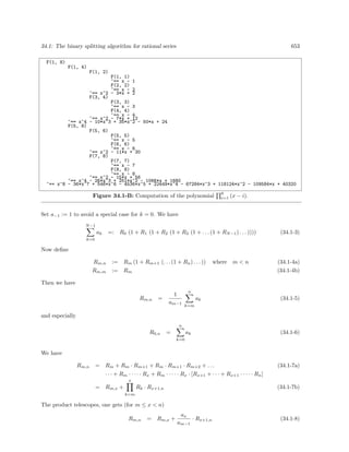


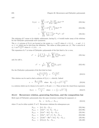


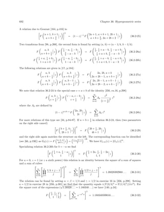


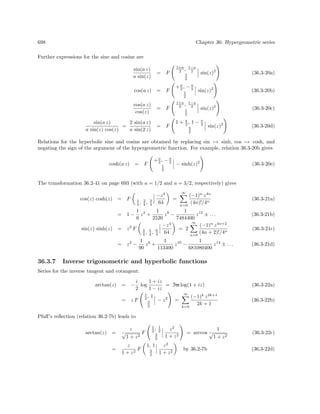


Algorithms for programers
- 1. Matters Computational Ideas, Algorithms, Source Code J¨org Arndt
- 2. ii
- 3. CONTENTS iii Contents Preface xi I Low level algorithms 1 1 Bit wizardry 2 1.1 Trivia . . . . . . . . . . . . . . . . . . . . . . . . . . . . . . . . . . . . . . . . . . . . . . . 2 1.2 Operations on individual bits . . . . . . . . . . . . . . . . . . . . . . . . . . . . . . . . . . 7 1.3 Operations on low bits or blocks of a word . . . . . . . . . . . . . . . . . . . . . . . . . . 8 1.4 Extraction of ones, zeros, or blocks near transitions . . . . . . . . . . . . . . . . . . . . . 11 1.5 Computing the index of a single set bit . . . . . . . . . . . . . . . . . . . . . . . . . . . . 13 1.6 Operations on high bits or blocks of a word . . . . . . . . . . . . . . . . . . . . . . . . . . 14 1.7 Functions related to the base-2 logarithm . . . . . . . . . . . . . . . . . . . . . . . . . . . 17 1.8 Counting the bits and blocks of a word . . . . . . . . . . . . . . . . . . . . . . . . . . . . 18 1.9 Words as bitsets . . . . . . . . . . . . . . . . . . . . . . . . . . . . . . . . . . . . . . . . . 23 1.10 Index of the i-th set bit . . . . . . . . . . . . . . . . . . . . . . . . . . . . . . . . . . . . . 25 1.11 Avoiding branches . . . . . . . . . . . . . . . . . . . . . . . . . . . . . . . . . . . . . . . . 25 1.12 Bit-wise rotation of a word . . . . . . . . . . . . . . . . . . . . . . . . . . . . . . . . . . . 27 1.13 Binary necklaces ‡ . . . . . . . . . . . . . . . . . . . . . . . . . . . . . . . . . . . . . . . . 29 1.14 Reversing the bits of a word . . . . . . . . . . . . . . . . . . . . . . . . . . . . . . . . . . 33 1.15 Bit-wise zip . . . . . . . . . . . . . . . . . . . . . . . . . . . . . . . . . . . . . . . . . . . . 38 1.16 Gray code and parity . . . . . . . . . . . . . . . . . . . . . . . . . . . . . . . . . . . . . . 41 1.17 Bit sequency ‡ . . . . . . . . . . . . . . . . . . . . . . . . . . . . . . . . . . . . . . . . . . 46 1.18 Powers of the Gray code ‡ . . . . . . . . . . . . . . . . . . . . . . . . . . . . . . . . . . . 48 1.19 Invertible transforms on words ‡ . . . . . . . . . . . . . . . . . . . . . . . . . . . . . . . . 49 1.20 Scanning for zero bytes . . . . . . . . . . . . . . . . . . . . . . . . . . . . . . . . . . . . . 55 1.21 Inverse and square root modulo 2n . . . . . . . . . . . . . . . . . . . . . . . . . . . . . . . 56 1.22 Radix −2 (minus two) representation . . . . . . . . . . . . . . . . . . . . . . . . . . . . . 58 1.23 A sparse signed binary representation . . . . . . . . . . . . . . . . . . . . . . . . . . . . . 61 1.24 Generating bit combinations . . . . . . . . . . . . . . . . . . . . . . . . . . . . . . . . . . 62 1.25 Generating bit subsets of a given word . . . . . . . . . . . . . . . . . . . . . . . . . . . . 68 1.26 Binary words in lexicographic order for subsets . . . . . . . . . . . . . . . . . . . . . . . . 70 1.27 Fibonacci words ‡ . . . . . . . . . . . . . . . . . . . . . . . . . . . . . . . . . . . . . . . . 74 1.28 Binary words and parentheses strings ‡ . . . . . . . . . . . . . . . . . . . . . . . . . . . . 78 1.29 Permutations via primitives ‡ . . . . . . . . . . . . . . . . . . . . . . . . . . . . . . . . . . 80 1.30 CPU instructions often missed . . . . . . . . . . . . . . . . . . . . . . . . . . . . . . . . . 82 1.31 Some space filling curves ‡ . . . . . . . . . . . . . . . . . . . . . . . . . . . . . . . . . . . 83 2 Permutations and their operations 102 2.1 Basic definitions and operations . . . . . . . . . . . . . . . . . . . . . . . . . . . . . . . . 102 2.2 Representation as disjoint cycles . . . . . . . . . . . . . . . . . . . . . . . . . . . . . . . . 104 2.3 Compositions of permutations . . . . . . . . . . . . . . . . . . . . . . . . . . . . . . . . . 105
- 4. iv CONTENTS 2.4 In-place methods to apply permutations to data . . . . . . . . . . . . . . . . . . . . . . . 109 2.5 Random permutations . . . . . . . . . . . . . . . . . . . . . . . . . . . . . . . . . . . . . . 111 2.6 The revbin permutation . . . . . . . . . . . . . . . . . . . . . . . . . . . . . . . . . . . . . 118 2.7 The radix permutation . . . . . . . . . . . . . . . . . . . . . . . . . . . . . . . . . . . . . 121 2.8 In-place matrix transposition . . . . . . . . . . . . . . . . . . . . . . . . . . . . . . . . . . 122 2.9 Rotation by triple reversal . . . . . . . . . . . . . . . . . . . . . . . . . . . . . . . . . . . 123 2.10 The zip permutation . . . . . . . . . . . . . . . . . . . . . . . . . . . . . . . . . . . . . . . 125 2.11 The XOR permutation . . . . . . . . . . . . . . . . . . . . . . . . . . . . . . . . . . . . . 127 2.12 The Gray permutation . . . . . . . . . . . . . . . . . . . . . . . . . . . . . . . . . . . . . 128 2.13 The reversed Gray permutation . . . . . . . . . . . . . . . . . . . . . . . . . . . . . . . . 131 3 Sorting and searching 134 3.1 Sorting algorithms . . . . . . . . . . . . . . . . . . . . . . . . . . . . . . . . . . . . . . . . 134 3.2 Binary search . . . . . . . . . . . . . . . . . . . . . . . . . . . . . . . . . . . . . . . . . . . 141 3.3 Variants of sorting methods . . . . . . . . . . . . . . . . . . . . . . . . . . . . . . . . . . . 142 3.4 Searching in unsorted arrays . . . . . . . . . . . . . . . . . . . . . . . . . . . . . . . . . . 147 3.5 Determination of equivalence classes . . . . . . . . . . . . . . . . . . . . . . . . . . . . . . 148 4 Data structures 153 4.1 Stack (LIFO) . . . . . . . . . . . . . . . . . . . . . . . . . . . . . . . . . . . . . . . . . . . 153 4.2 Ring buffer . . . . . . . . . . . . . . . . . . . . . . . . . . . . . . . . . . . . . . . . . . . . 155 4.3 Queue (FIFO) . . . . . . . . . . . . . . . . . . . . . . . . . . . . . . . . . . . . . . . . . . 156 4.4 Deque (double-ended queue) . . . . . . . . . . . . . . . . . . . . . . . . . . . . . . . . . . 158 4.5 Heap and priority queue . . . . . . . . . . . . . . . . . . . . . . . . . . . . . . . . . . . . . 160 4.6 Bit-array . . . . . . . . . . . . . . . . . . . . . . . . . . . . . . . . . . . . . . . . . . . . . 164 4.7 Left-right array . . . . . . . . . . . . . . . . . . . . . . . . . . . . . . . . . . . . . . . . . 166 II Combinatorial generation 171 5 Conventions and considerations 172 5.1 Representations and orders . . . . . . . . . . . . . . . . . . . . . . . . . . . . . . . . . . . 172 5.2 Ranking, unranking, and counting . . . . . . . . . . . . . . . . . . . . . . . . . . . . . . . 172 5.3 Characteristics of the algorithms . . . . . . . . . . . . . . . . . . . . . . . . . . . . . . . . 173 5.4 Optimization techniques . . . . . . . . . . . . . . . . . . . . . . . . . . . . . . . . . . . . . 174 5.5 Implementations, demo-programs, and timings . . . . . . . . . . . . . . . . . . . . . . . . 174 6 Combinations 176 6.1 Binomial coefficients . . . . . . . . . . . . . . . . . . . . . . . . . . . . . . . . . . . . . . . 176 6.2 Lexicographic and co-lexicographic order . . . . . . . . . . . . . . . . . . . . . . . . . . . 177 6.3 Order by prefix shifts (cool-lex) . . . . . . . . . . . . . . . . . . . . . . . . . . . . . . . . 180 6.4 Minimal-change order . . . . . . . . . . . . . . . . . . . . . . . . . . . . . . . . . . . . . . 182 6.5 The Eades-McKay strong minimal-change order . . . . . . . . . . . . . . . . . . . . . . . 183 6.6 Two-close orderings via endo/enup moves . . . . . . . . . . . . . . . . . . . . . . . . . . . 186 6.7 Recursive generation of certain orderings . . . . . . . . . . . . . . . . . . . . . . . . . . . 191 7 Compositions 194 7.1 Co-lexicographic order . . . . . . . . . . . . . . . . . . . . . . . . . . . . . . . . . . . . . . 194 7.2 Co-lexicographic order for compositions into exactly k parts . . . . . . . . . . . . . . . . 196 7.3 Compositions and combinations . . . . . . . . . . . . . . . . . . . . . . . . . . . . . . . . 198 7.4 Minimal-change orders . . . . . . . . . . . . . . . . . . . . . . . . . . . . . . . . . . . . . 199 8 Subsets 202 8.1 Lexicographic order . . . . . . . . . . . . . . . . . . . . . . . . . . . . . . . . . . . . . . . 202 8.2 Minimal-change order . . . . . . . . . . . . . . . . . . . . . . . . . . . . . . . . . . . . . . 204
- 5. CONTENTS v 8.3 Ordering with De Bruijn sequences . . . . . . . . . . . . . . . . . . . . . . . . . . . . . . 208 8.4 Shifts-order for subsets . . . . . . . . . . . . . . . . . . . . . . . . . . . . . . . . . . . . . 208 8.5 k-subsets where k lies in a given range . . . . . . . . . . . . . . . . . . . . . . . . . . . . . 210 9 Mixed radix numbers 217 9.1 Counting (lexicographic) order . . . . . . . . . . . . . . . . . . . . . . . . . . . . . . . . . 217 9.2 Minimal-change (Gray code) order . . . . . . . . . . . . . . . . . . . . . . . . . . . . . . . 220 9.3 gslex order . . . . . . . . . . . . . . . . . . . . . . . . . . . . . . . . . . . . . . . . . . . . 224 9.4 endo order . . . . . . . . . . . . . . . . . . . . . . . . . . . . . . . . . . . . . . . . . . . . 226 9.5 Gray code for endo order . . . . . . . . . . . . . . . . . . . . . . . . . . . . . . . . . . . . 228 9.6 Fixed sum of digits . . . . . . . . . . . . . . . . . . . . . . . . . . . . . . . . . . . . . . . 229 10 Permutations 232 10.1 Factorial representations of permutations . . . . . . . . . . . . . . . . . . . . . . . . . . . 232 10.2 Lexicographic order . . . . . . . . . . . . . . . . . . . . . . . . . . . . . . . . . . . . . . . 242 10.3 Co-lexicographic order . . . . . . . . . . . . . . . . . . . . . . . . . . . . . . . . . . . . . . 243 10.4 An order from reversing prefixes . . . . . . . . . . . . . . . . . . . . . . . . . . . . . . . . 245 10.5 Minimal-change order (Heap’s algorithm) . . . . . . . . . . . . . . . . . . . . . . . . . . . 248 10.6 Lipski’s Minimal-change orders . . . . . . . . . . . . . . . . . . . . . . . . . . . . . . . . . 250 10.7 Strong minimal-change order (Trotter’s algorithm) . . . . . . . . . . . . . . . . . . . . . . 254 10.8 Star-transposition order . . . . . . . . . . . . . . . . . . . . . . . . . . . . . . . . . . . . . 257 10.9 Minimal-change orders from factorial numbers . . . . . . . . . . . . . . . . . . . . . . . . 258 10.10 Derangement order . . . . . . . . . . . . . . . . . . . . . . . . . . . . . . . . . . . . . . . 264 10.11 Orders where the smallest element always moves right . . . . . . . . . . . . . . . . . . . . 267 10.12 Single track orders . . . . . . . . . . . . . . . . . . . . . . . . . . . . . . . . . . . . . . . . 271 11 Permutations with special properties 277 11.1 The number of certain permutations . . . . . . . . . . . . . . . . . . . . . . . . . . . . . . 277 11.2 Permutations with distance restrictions . . . . . . . . . . . . . . . . . . . . . . . . . . . . 282 11.3 Self-inverse permutations (involutions) . . . . . . . . . . . . . . . . . . . . . . . . . . . . . 284 11.4 Cyclic permutations . . . . . . . . . . . . . . . . . . . . . . . . . . . . . . . . . . . . . . . 285 12 k-permutations 291 12.1 Lexicographic order . . . . . . . . . . . . . . . . . . . . . . . . . . . . . . . . . . . . . . . 292 12.2 Minimal-change order . . . . . . . . . . . . . . . . . . . . . . . . . . . . . . . . . . . . . . 293 13 Multisets 295 13.1 Subsets of a multiset . . . . . . . . . . . . . . . . . . . . . . . . . . . . . . . . . . . . . . 295 13.2 Permutations of a multiset . . . . . . . . . . . . . . . . . . . . . . . . . . . . . . . . . . . 296 14 Gray codes for strings with restrictions 304 14.1 List recursions . . . . . . . . . . . . . . . . . . . . . . . . . . . . . . . . . . . . . . . . . . 304 14.2 Fibonacci words . . . . . . . . . . . . . . . . . . . . . . . . . . . . . . . . . . . . . . . . . 305 14.3 Generalized Fibonacci words . . . . . . . . . . . . . . . . . . . . . . . . . . . . . . . . . . 307 14.4 Run-length limited (RLL) words . . . . . . . . . . . . . . . . . . . . . . . . . . . . . . . . 310 14.5 Digit x followed by at least x zeros . . . . . . . . . . . . . . . . . . . . . . . . . . . . . . . 311 14.6 Generalized Pell words . . . . . . . . . . . . . . . . . . . . . . . . . . . . . . . . . . . . . 313 14.7 Sparse signed binary words . . . . . . . . . . . . . . . . . . . . . . . . . . . . . . . . . . . 315 14.8 Strings with no two consecutive nonzero digits . . . . . . . . . . . . . . . . . . . . . . . . 317 14.9 Strings with no two consecutive zeros . . . . . . . . . . . . . . . . . . . . . . . . . . . . . 318 14.10 Binary strings without substrings 1x1 or 1xy1 ‡ . . . . . . . . . . . . . . . . . . . . . . . 320 15 Parentheses strings 323 15.1 Co-lexicographic order . . . . . . . . . . . . . . . . . . . . . . . . . . . . . . . . . . . . . . 323 15.2 Gray code via restricted growth strings . . . . . . . . . . . . . . . . . . . . . . . . . . . . 325
- 6. vi CONTENTS 15.3 Order by prefix shifts (cool-lex) . . . . . . . . . . . . . . . . . . . . . . . . . . . . . . . . 330 15.4 Catalan numbers . . . . . . . . . . . . . . . . . . . . . . . . . . . . . . . . . . . . . . . . . 331 15.5 Increment-i RGS, k-ary Dyck words, and k-ary trees . . . . . . . . . . . . . . . . . . . . . 333 16 Integer partitions 339 16.1 Solution of a generalized problem . . . . . . . . . . . . . . . . . . . . . . . . . . . . . . . 339 16.2 Iterative algorithm . . . . . . . . . . . . . . . . . . . . . . . . . . . . . . . . . . . . . . . . 341 16.3 Partitions into m parts . . . . . . . . . . . . . . . . . . . . . . . . . . . . . . . . . . . . . 342 16.4 The number of integer partitions . . . . . . . . . . . . . . . . . . . . . . . . . . . . . . . . 344 17 Set partitions 354 17.1 Recursive generation . . . . . . . . . . . . . . . . . . . . . . . . . . . . . . . . . . . . . . . 354 17.2 The number of set partitions: Stirling set numbers and Bell numbers . . . . . . . . . . . 358 17.3 Restricted growth strings . . . . . . . . . . . . . . . . . . . . . . . . . . . . . . . . . . . . 360 18 Necklaces and Lyndon words 370 18.1 Generating all necklaces . . . . . . . . . . . . . . . . . . . . . . . . . . . . . . . . . . . . . 371 18.2 Lex-min De Bruijn sequence from necklaces . . . . . . . . . . . . . . . . . . . . . . . . . . 377 18.3 The number of binary necklaces . . . . . . . . . . . . . . . . . . . . . . . . . . . . . . . . 379 18.4 Sums of roots of unity that are zero ‡ . . . . . . . . . . . . . . . . . . . . . . . . . . . . . 383 19 Hadamard and conference matrices 384 19.1 Hadamard matrices via LFSR . . . . . . . . . . . . . . . . . . . . . . . . . . . . . . . . . 384 19.2 Hadamard matrices via conference matrices . . . . . . . . . . . . . . . . . . . . . . . . . . 386 19.3 Conference matrices via finite fields . . . . . . . . . . . . . . . . . . . . . . . . . . . . . . 388 20 Searching paths in directed graphs ‡ 391 20.1 Representation of digraphs . . . . . . . . . . . . . . . . . . . . . . . . . . . . . . . . . . . 392 20.2 Searching full paths . . . . . . . . . . . . . . . . . . . . . . . . . . . . . . . . . . . . . . . 393 20.3 Conditional search . . . . . . . . . . . . . . . . . . . . . . . . . . . . . . . . . . . . . . . . 398 20.4 Edge sorting and lucky paths . . . . . . . . . . . . . . . . . . . . . . . . . . . . . . . . . . 402 20.5 Gray codes for Lyndon words . . . . . . . . . . . . . . . . . . . . . . . . . . . . . . . . . . 403 III Fast transforms 409 21 The Fourier transform 410 21.1 The discrete Fourier transform . . . . . . . . . . . . . . . . . . . . . . . . . . . . . . . . . 410 21.2 Radix-2 FFT algorithms . . . . . . . . . . . . . . . . . . . . . . . . . . . . . . . . . . . . 411 21.3 Saving trigonometric computations . . . . . . . . . . . . . . . . . . . . . . . . . . . . . . 416 21.4 Higher radix FFT algorithms . . . . . . . . . . . . . . . . . . . . . . . . . . . . . . . . . . 418 21.5 Split-radix algorithm . . . . . . . . . . . . . . . . . . . . . . . . . . . . . . . . . . . . . . 425 21.6 Symmetries of the Fourier transform . . . . . . . . . . . . . . . . . . . . . . . . . . . . . . 428 21.7 Inverse FFT for free . . . . . . . . . . . . . . . . . . . . . . . . . . . . . . . . . . . . . . . 430 21.8 Real-valued Fourier transforms . . . . . . . . . . . . . . . . . . . . . . . . . . . . . . . . . 431 21.9 Multi-dimensional Fourier transforms . . . . . . . . . . . . . . . . . . . . . . . . . . . . . 437 21.10 The matrix Fourier algorithm (MFA) . . . . . . . . . . . . . . . . . . . . . . . . . . . . . 438 22 Convolution, correlation, and more FFT algorithms 440 22.1 Convolution . . . . . . . . . . . . . . . . . . . . . . . . . . . . . . . . . . . . . . . . . . . 440 22.2 Correlation . . . . . . . . . . . . . . . . . . . . . . . . . . . . . . . . . . . . . . . . . . . . 444 22.3 Correlation, convolution, and circulant matrices ‡ . . . . . . . . . . . . . . . . . . . . . . 447 22.4 Weighted Fourier transforms and convolutions . . . . . . . . . . . . . . . . . . . . . . . . 448 22.5 Convolution using the MFA . . . . . . . . . . . . . . . . . . . . . . . . . . . . . . . . . . . 451 22.6 The z-transform (ZT) . . . . . . . . . . . . . . . . . . . . . . . . . . . . . . . . . . . . . . 454
- 7. CONTENTS vii 22.7 Prime length FFTs . . . . . . . . . . . . . . . . . . . . . . . . . . . . . . . . . . . . . . . 457 23 The Walsh transform and its relatives 459 23.1 Transform with Walsh-Kronecker basis . . . . . . . . . . . . . . . . . . . . . . . . . . . . 459 23.2 Eigenvectors of the Walsh transform ‡ . . . . . . . . . . . . . . . . . . . . . . . . . . . . . 461 23.3 The Kronecker product . . . . . . . . . . . . . . . . . . . . . . . . . . . . . . . . . . . . . 462 23.4 Higher radix Walsh transforms . . . . . . . . . . . . . . . . . . . . . . . . . . . . . . . . . 465 23.5 Localized Walsh transforms . . . . . . . . . . . . . . . . . . . . . . . . . . . . . . . . . . . 468 23.6 Transform with Walsh-Paley basis . . . . . . . . . . . . . . . . . . . . . . . . . . . . . . . 473 23.7 Sequency-ordered Walsh transforms . . . . . . . . . . . . . . . . . . . . . . . . . . . . . . 474 23.8 XOR (dyadic) convolution . . . . . . . . . . . . . . . . . . . . . . . . . . . . . . . . . . . 481 23.9 Slant transform . . . . . . . . . . . . . . . . . . . . . . . . . . . . . . . . . . . . . . . . . 482 23.10 Arithmetic transform . . . . . . . . . . . . . . . . . . . . . . . . . . . . . . . . . . . . . . 483 23.11 Reed-Muller transform . . . . . . . . . . . . . . . . . . . . . . . . . . . . . . . . . . . . . 486 23.12 The OR-convolution and the AND-convolution . . . . . . . . . . . . . . . . . . . . . . . . 489 23.13 The MAX-convolution ‡ . . . . . . . . . . . . . . . . . . . . . . . . . . . . . . . . . . . . . 491 23.14 Weighted arithmetic transform and subset convolution . . . . . . . . . . . . . . . . . . . . 492 24 The Haar transform 497 24.1 The ‘standard’ Haar transform . . . . . . . . . . . . . . . . . . . . . . . . . . . . . . . . . 497 24.2 In-place Haar transform . . . . . . . . . . . . . . . . . . . . . . . . . . . . . . . . . . . . . 499 24.3 Non-normalized Haar transforms . . . . . . . . . . . . . . . . . . . . . . . . . . . . . . . . 501 24.4 Transposed Haar transforms ‡ . . . . . . . . . . . . . . . . . . . . . . . . . . . . . . . . . 503 24.5 The reversed Haar transform ‡ . . . . . . . . . . . . . . . . . . . . . . . . . . . . . . . . . 505 24.6 Relations between Walsh and Haar transforms . . . . . . . . . . . . . . . . . . . . . . . . 507 24.7 Prefix transform and prefix convolution . . . . . . . . . . . . . . . . . . . . . . . . . . . . 510 24.8 Nonstandard splitting schemes ‡ . . . . . . . . . . . . . . . . . . . . . . . . . . . . . . . . 512 25 The Hartley transform 515 25.1 Definition and symmetries . . . . . . . . . . . . . . . . . . . . . . . . . . . . . . . . . . . 515 25.2 Radix-2 FHT algorithms . . . . . . . . . . . . . . . . . . . . . . . . . . . . . . . . . . . . 515 25.3 Complex FFT by FHT . . . . . . . . . . . . . . . . . . . . . . . . . . . . . . . . . . . . . 521 25.4 Complex FFT by complex FHT and vice versa . . . . . . . . . . . . . . . . . . . . . . . . 522 25.5 Real FFT by FHT and vice versa . . . . . . . . . . . . . . . . . . . . . . . . . . . . . . . 523 25.6 Higher radix FHT algorithms . . . . . . . . . . . . . . . . . . . . . . . . . . . . . . . . . . 524 25.7 Convolution via FHT . . . . . . . . . . . . . . . . . . . . . . . . . . . . . . . . . . . . . . 525 25.8 Localized FHT algorithms . . . . . . . . . . . . . . . . . . . . . . . . . . . . . . . . . . . 529 25.9 2-dimensional FHTs . . . . . . . . . . . . . . . . . . . . . . . . . . . . . . . . . . . . . . . 530 25.10 Automatic generation of transform code . . . . . . . . . . . . . . . . . . . . . . . . . . . . 531 25.11 Eigenvectors of the Fourier and Hartley transform ‡ . . . . . . . . . . . . . . . . . . . . . 533 26 Number theoretic transforms (NTTs) 535 26.1 Prime moduli for NTTs . . . . . . . . . . . . . . . . . . . . . . . . . . . . . . . . . . . . . 535 26.2 Implementation of NTTs . . . . . . . . . . . . . . . . . . . . . . . . . . . . . . . . . . . . 537 26.3 Convolution with NTTs . . . . . . . . . . . . . . . . . . . . . . . . . . . . . . . . . . . . . 542 27 Fast wavelet transforms 543 27.1 Wavelet filters . . . . . . . . . . . . . . . . . . . . . . . . . . . . . . . . . . . . . . . . . . 543 27.2 Implementation . . . . . . . . . . . . . . . . . . . . . . . . . . . . . . . . . . . . . . . . . 544 27.3 Moment conditions . . . . . . . . . . . . . . . . . . . . . . . . . . . . . . . . . . . . . . . 546 IV Fast arithmetic 549 28 Fast multiplication and exponentiation 550
- 8. viii CONTENTS 28.1 Splitting schemes for multiplication . . . . . . . . . . . . . . . . . . . . . . . . . . . . . . 550 28.2 Fast multiplication via FFT . . . . . . . . . . . . . . . . . . . . . . . . . . . . . . . . . . 558 28.3 Radix/precision considerations with FFT multiplication . . . . . . . . . . . . . . . . . . . 560 28.4 The sum-of-digits test . . . . . . . . . . . . . . . . . . . . . . . . . . . . . . . . . . . . . . 562 28.5 Binary exponentiation . . . . . . . . . . . . . . . . . . . . . . . . . . . . . . . . . . . . . . 563 29 Root extraction 567 29.1 Division, square root and cube root . . . . . . . . . . . . . . . . . . . . . . . . . . . . . . 567 29.2 Root extraction for rationals . . . . . . . . . . . . . . . . . . . . . . . . . . . . . . . . . . 570 29.3 Divisionless iterations for the inverse a-th root . . . . . . . . . . . . . . . . . . . . . . . . 572 29.4 Initial approximations for iterations . . . . . . . . . . . . . . . . . . . . . . . . . . . . . . 575 29.5 Some applications of the matrix square root . . . . . . . . . . . . . . . . . . . . . . . . . 576 29.6 Goldschmidt’s algorithm . . . . . . . . . . . . . . . . . . . . . . . . . . . . . . . . . . . . 581 29.7 Products for the a-th root ‡ . . . . . . . . . . . . . . . . . . . . . . . . . . . . . . . . . . 583 29.8 Divisionless iterations for polynomial roots . . . . . . . . . . . . . . . . . . . . . . . . . . 586 30 Iterations for the inversion of a function 587 30.1 Iterations and their rate of convergence . . . . . . . . . . . . . . . . . . . . . . . . . . . . 587 30.2 Schr¨oder’s formula . . . . . . . . . . . . . . . . . . . . . . . . . . . . . . . . . . . . . . . . 588 30.3 Householder’s formula . . . . . . . . . . . . . . . . . . . . . . . . . . . . . . . . . . . . . . 592 30.4 Dealing with multiple roots . . . . . . . . . . . . . . . . . . . . . . . . . . . . . . . . . . . 593 30.5 More iterations . . . . . . . . . . . . . . . . . . . . . . . . . . . . . . . . . . . . . . . . . . 594 30.6 Convergence improvement by the delta squared process . . . . . . . . . . . . . . . . . . . 598 31 The AGM, elliptic integrals, and algorithms for computing π 599 31.1 The arithmetic-geometric mean (AGM) . . . . . . . . . . . . . . . . . . . . . . . . . . . . 599 31.2 The elliptic integrals K and E . . . . . . . . . . . . . . . . . . . . . . . . . . . . . . . . . 600 31.3 Theta functions, eta functions, and singular values . . . . . . . . . . . . . . . . . . . . . . 604 31.4 AGM-type algorithms for hypergeometric functions . . . . . . . . . . . . . . . . . . . . . 611 31.5 Computation of π . . . . . . . . . . . . . . . . . . . . . . . . . . . . . . . . . . . . . . . . 615 32 Logarithm and exponential function 622 32.1 Logarithm . . . . . . . . . . . . . . . . . . . . . . . . . . . . . . . . . . . . . . . . . . . . 622 32.2 Exponential function . . . . . . . . . . . . . . . . . . . . . . . . . . . . . . . . . . . . . . 627 32.3 Logarithm and exponential function of power series . . . . . . . . . . . . . . . . . . . . . 630 32.4 Simultaneous computation of logarithms of small primes . . . . . . . . . . . . . . . . . . 632 32.5 Arctangent relations for π ‡ . . . . . . . . . . . . . . . . . . . . . . . . . . . . . . . . . . . 633 33 Computing the elementary functions with limited resources 641 33.1 Shift-and-add algorithms for logb(x) and bx . . . . . . . . . . . . . . . . . . . . . . . . . . 641 33.2 CORDIC algorithms . . . . . . . . . . . . . . . . . . . . . . . . . . . . . . . . . . . . . . . 646 34 Numerical evaluation of power series 651 34.1 The binary splitting algorithm for rational series . . . . . . . . . . . . . . . . . . . . . . . 651 34.2 Rectangular schemes for evaluation of power series . . . . . . . . . . . . . . . . . . . . . . 658 34.3 The magic sumalt algorithm for alternating series . . . . . . . . . . . . . . . . . . . . . . 662 35 Recurrences and Chebyshev polynomials 666 35.1 Recurrences . . . . . . . . . . . . . . . . . . . . . . . . . . . . . . . . . . . . . . . . . . . 666 35.2 Chebyshev polynomials . . . . . . . . . . . . . . . . . . . . . . . . . . . . . . . . . . . . . 676 36 Hypergeometric series 685 36.1 Definition and basic operations . . . . . . . . . . . . . . . . . . . . . . . . . . . . . . . . . 685 36.2 Transformations of hypergeometric series . . . . . . . . . . . . . . . . . . . . . . . . . . . 688 36.3 Examples: elementary functions . . . . . . . . . . . . . . . . . . . . . . . . . . . . . . . . 694
- 9. CONTENTS ix 36.4 Transformations for elliptic integrals ‡ . . . . . . . . . . . . . . . . . . . . . . . . . . . . . 700 36.5 The function xx ‡ . . . . . . . . . . . . . . . . . . . . . . . . . . . . . . . . . . . . . . . . 702 37 Cyclotomic polynomials, product forms, and continued fractions 704 37.1 Cyclotomic polynomials, M¨obius inversion, Lambert series . . . . . . . . . . . . . . . . . 704 37.2 Conversion of power series to infinite products . . . . . . . . . . . . . . . . . . . . . . . . 709 37.3 Continued fractions . . . . . . . . . . . . . . . . . . . . . . . . . . . . . . . . . . . . . . . 716 38 Synthetic Iterations ‡ 726 38.1 A variation of the iteration for the inverse . . . . . . . . . . . . . . . . . . . . . . . . . . . 726 38.2 An iteration related to the Thue constant . . . . . . . . . . . . . . . . . . . . . . . . . . . 730 38.3 An iteration related to the Golay-Rudin-Shapiro sequence . . . . . . . . . . . . . . . . . . 731 38.4 Iteration related to the ruler function . . . . . . . . . . . . . . . . . . . . . . . . . . . . . 733 38.5 An iteration related to the period-doubling sequence . . . . . . . . . . . . . . . . . . . . . 734 38.6 An iteration from substitution rules with sign . . . . . . . . . . . . . . . . . . . . . . . . 738 38.7 Iterations related to the sum of digits . . . . . . . . . . . . . . . . . . . . . . . . . . . . . 739 38.8 Iterations related to the binary Gray code . . . . . . . . . . . . . . . . . . . . . . . . . . . 741 38.9 A function encoding the Hilbert curve . . . . . . . . . . . . . . . . . . . . . . . . . . . . . 747 38.10 Sparse power series . . . . . . . . . . . . . . . . . . . . . . . . . . . . . . . . . . . . . . . 750 38.11 An iteration related to the Fibonacci numbers . . . . . . . . . . . . . . . . . . . . . . . . 753 38.12 Iterations related to the Pell numbers . . . . . . . . . . . . . . . . . . . . . . . . . . . . . 757 V Algorithms for finite fields 763 39 Modular arithmetic and some number theory 764 39.1 Implementation of the arithmetic operations . . . . . . . . . . . . . . . . . . . . . . . . . 764 39.2 Modular reduction with structured primes . . . . . . . . . . . . . . . . . . . . . . . . . . 768 39.3 The sieve of Eratosthenes . . . . . . . . . . . . . . . . . . . . . . . . . . . . . . . . . . . . 770 39.4 The Chinese Remainder Theorem (CRT) . . . . . . . . . . . . . . . . . . . . . . . . . . . 772 39.5 The order of an element . . . . . . . . . . . . . . . . . . . . . . . . . . . . . . . . . . . . . 774 39.6 Prime modulus: the field Z/pZ = Fp = GF(p) . . . . . . . . . . . . . . . . . . . . . . . . 776 39.7 Composite modulus: the ring Z/mZ . . . . . . . . . . . . . . . . . . . . . . . . . . . . . . 776 39.8 Quadratic residues . . . . . . . . . . . . . . . . . . . . . . . . . . . . . . . . . . . . . . . . 781 39.9 Computation of a square root modulo m . . . . . . . . . . . . . . . . . . . . . . . . . . . 784 39.10 The Rabin-Miller test for compositeness . . . . . . . . . . . . . . . . . . . . . . . . . . . . 786 39.11 Proving primality . . . . . . . . . . . . . . . . . . . . . . . . . . . . . . . . . . . . . . . . 792 39.12 Complex modulus: the field GF(p2 ) . . . . . . . . . . . . . . . . . . . . . . . . . . . . . . 804 39.13 Solving the Pell equation . . . . . . . . . . . . . . . . . . . . . . . . . . . . . . . . . . . . 812 39.14 Multiplication of hypercomplex numbers ‡ . . . . . . . . . . . . . . . . . . . . . . . . . . 815 40 Binary polynomials 822 40.1 The basic arithmetical operations . . . . . . . . . . . . . . . . . . . . . . . . . . . . . . . 822 40.2 Multiplying binary polynomials of high degree . . . . . . . . . . . . . . . . . . . . . . . . 827 40.3 Modular arithmetic with binary polynomials . . . . . . . . . . . . . . . . . . . . . . . . . 832 40.4 Irreducible polynomials . . . . . . . . . . . . . . . . . . . . . . . . . . . . . . . . . . . . . 837 40.5 Primitive polynomials . . . . . . . . . . . . . . . . . . . . . . . . . . . . . . . . . . . . . . 841 40.6 The number of irreducible and primitive polynomials . . . . . . . . . . . . . . . . . . . . 843 40.7 Transformations that preserve irreducibility . . . . . . . . . . . . . . . . . . . . . . . . . . 845 40.8 Self-reciprocal polynomials . . . . . . . . . . . . . . . . . . . . . . . . . . . . . . . . . . . 846 40.9 Irreducible and primitive polynomials of special forms ‡ . . . . . . . . . . . . . . . . . . . 848 40.10 Generating irreducible polynomials from Lyndon words . . . . . . . . . . . . . . . . . . . 856 40.11 Irreducible and cyclotomic polynomials ‡ . . . . . . . . . . . . . . . . . . . . . . . . . . . 857 40.12 Factorization of binary polynomials . . . . . . . . . . . . . . . . . . . . . . . . . . . . . . 858
- 10. x CONTENTS 41 Shift registers 864 41.1 Linear feedback shift registers (LFSR) . . . . . . . . . . . . . . . . . . . . . . . . . . . . . 864 41.2 Galois and Fibonacci setup . . . . . . . . . . . . . . . . . . . . . . . . . . . . . . . . . . . 867 41.3 Error detection by hashing: the CRC . . . . . . . . . . . . . . . . . . . . . . . . . . . . . 868 41.4 Generating all revbin pairs . . . . . . . . . . . . . . . . . . . . . . . . . . . . . . . . . . . 873 41.5 The number of m-sequences and De Bruijn sequences . . . . . . . . . . . . . . . . . . . . 873 41.6 Auto-correlation of m-sequences . . . . . . . . . . . . . . . . . . . . . . . . . . . . . . . . 875 41.7 Feedback carry shift registers (FCSR) . . . . . . . . . . . . . . . . . . . . . . . . . . . . . 876 41.8 Linear hybrid cellular automata (LHCA) . . . . . . . . . . . . . . . . . . . . . . . . . . . 878 41.9 Additive linear hybrid cellular automata . . . . . . . . . . . . . . . . . . . . . . . . . . . 882 42 Binary finite fields: GF(2n ) 886 42.1 Arithmetic and basic properties . . . . . . . . . . . . . . . . . . . . . . . . . . . . . . . . 886 42.2 Minimal polynomials . . . . . . . . . . . . . . . . . . . . . . . . . . . . . . . . . . . . . . 892 42.3 Fast computation of the trace vector . . . . . . . . . . . . . . . . . . . . . . . . . . . . . . 895 42.4 Solving quadratic equations . . . . . . . . . . . . . . . . . . . . . . . . . . . . . . . . . . . 896 42.5 Representation by matrices ‡ . . . . . . . . . . . . . . . . . . . . . . . . . . . . . . . . . . 899 42.6 Representation by normal bases . . . . . . . . . . . . . . . . . . . . . . . . . . . . . . . . 900 42.7 Conversion between normal and polynomial representation . . . . . . . . . . . . . . . . . 910 42.8 Optimal normal bases (ONB) . . . . . . . . . . . . . . . . . . . . . . . . . . . . . . . . . . 912 42.9 Gaussian normal bases . . . . . . . . . . . . . . . . . . . . . . . . . . . . . . . . . . . . . 914 A The electronic version of the book 921 B Machine used for benchmarking 922 C The GP language 923 Bibliography 931 Index 951
- 11. Preface This is a book for the computationalist, whether a working programmer or anyone interested in methods of computation. The focus is on material that does not usually appear in textbooks on algorithms. Where necessary the underlying ideas are explained and the algorithms are given formally. It is assumed that the reader is able to understand the given source code, it is considered part of the text. We use the C++ programming language for low-level algorithms. However, only a minimal set of features beyond plain C is used, most importantly classes and templates. For material where technicalities in the C++ code would obscure the underlying ideas we use either pseudocode or, with arithmetical algorithms, the GP language. Appendix C gives an introduction to GP. Example computations are often given with an algorithm, these are usually made with the demo programs referred to. Most of the listings and figures in this book were created with these programs. A recurring topic is practical efficiency of the implementations. Various optimization techniques are described and the actual performance of many given implementations is indicated. The accompanying software, the FXT [21] and the hfloat [22] libraries, are written for POSIX compliant platforms such as the Linux and BSD operating systems. The license is the GNU General Public License (GPL), version 3 or later, see http://www.gnu.org/licenses/gpl.html. Individual chapters are self-contained where possible and references to related material are given where needed. The symbol ‘ ‡ ’ marks sections that can be skipped at first reading. These typically contain excursions or more advanced material. Each item in the bibliography is followed by a list of page numbers where citations occur. With papers that are available for free download the respective URL is given. Note that the URL may point to a preprint which can differ from the final version of the paper. An electronic version of this book is available online, see appendix A. Given the amount of material treated there must be errors in this book. Corrections and suggestions for improvement are appreciated, the preferred way of communication is electronic mail. A list of errata is online at http://www.jjj.de/ fxt/#fxtbook. Many people helped to improve this book. It is my pleasure to thank them all, particularly helpful were Igal Aharonovich, Max Alekseyev, Marcus Blackburn, Nathan Bullock, Dominique Delande, Mike Engber, Torsten Finke, Sean Furlong, Almaz Gaifullin, Pedro Gimeno, Alexander Gly- zov, R. W. Gosper, Andreas Gr¨unbacher, Lance Gurney, Markus Gyger, Christoph Haenel, Tony Hardie-Bick, Laszlo Hars, Thomas Harte, Stephen Hartke, Christian Hey, Jeff Hurchalla, Derek M. Jones, Gideon Klimer, Richard B. Kreckel, Mike Kundmann, G´al L´aszl´o, Dirk Lat- termann, Avery Lee, Brent Lehman, Marc Lehmann, Paul C. Leopardi, John Lien, Mirko Liss, Robert C. Long, Fred Lunnon, Johannes Middeke, Doug Moore, F´abio Moreira, Andrew Morris, David Nalepa, Samuel Neves, Matthew Oliver, Miroslaw Osys, Christoph Pacher, Kriszti´an Pacz´ari, Scott Paine, Yves Paradis, Gunther Piez, Andr´e Piotrowski, David Garc´ıa Quintas, Andreas Raseghi, Tony Reix, Johan R¨onnblom, Uwe Schmelich, Thomas Schraitle, Clive Scott, Mukund Sivaraman, Michal Staruch, Ralf Stephan, Mikko Tommila, Sebastiano
- 12. Vigna, Michael Roby Wetherfield, Jim White, Vinnie Winkler, John Youngquist, Rui Zhang, and Paul Zimmermann. Special thanks go to Edith Parzefall and Michael Somos for independently proofreading the whole text (the remaining errors are mine), and to Neil Sloane for creating the On-Line Encyclopedia of Integer Sequences [312]. jj N¨urnberg, Germany, June 2010 “Why make things difficult, when it is possible to make them cryptic and totally illogical, with just a little bit more effort?” — Aksel Peter Jørgensen
- 13. 1 Part I Low level algorithms
- 14. 2 Chapter 1: Bit wizardry Chapter 1 Bit wizardry We give low-level functions for binary words, such as isolation of the lowest set bit or counting all set bits. Sometimes the term ‘one’ is used for a set bit and ‘zero’ for an unset bit. Where it cannot cause confusion, the term ‘bit’ is used for a set bit (as in “counting the bits of a word”). The C-type unsigned long is abbreviated as ulong as defined in [FXT: fxttypes.h]. It is assumed that BITS_PER_LONG reflects the size of an unsigned long. It is defined in [FXT: bits/bitsperlong.h] and usually equals the machine word size: 32 on 32-bit architectures, and 64 on 64-bit machines. Further, the quantity BYTES_PER_LONG reflects the number of bytes in a machine word: it equals BITS_PER_LONG divided by eight. For some functions it is assumed that long and ulong have the same number of bits. Many functions will only work on machines that use two’s complement, which is used by all of the current general purpose computers (the only machines using one’s complement appear to be some successors of the UNIVAC system, see [358, entry “UNIVAC 1100/2200 series”]). The examples of assembler code are for the x86 and the AMD64 architecture. They should be simple enough to be understood by readers who know assembler for any CPU. 1.1 Trivia 1.1.1 Little endian versus big endian The order in which the bytes of an integer are stored in memory can start with the least significant byte (little endian machine) or with the most significant byte (big endian machine). The hexadecimal number 0x0D0C0B0A will be stored in the following manner if memory addresses grow from left to right: adr: z z+1 z+2 z+3 mem: 0D 0C 0B 0A // big endian mem: 0A 0B 0C 0D // little endian The difference becomes visible when you cast pointers. Let V be the 32-bit integer with the value above. Then the result of char c = *(char *)(&V); will be 0x0A (value modulo 256) on a little endian machine but 0x0D (value divided by 224 ) on a big endian machine. Though friends of big endian sometimes refer to little endian as ‘wrong endian’, the desired result of the shown pointer cast is much more often the modulo operation. Whenever words are serialized into bytes, as with transfer over a network or to a disk, one will need two code versions, one for big endian and one for little endian machines. The C-type union (with words and bytes) may also require separate treatment for big and little endian architectures. 1.1.2 Size of pointer is not size of int If programming for a 32-bit architecture (where the size of int and long coincide), casting pointers to integers (and back) will usually work. The same code will fail on 64-bit machines. If you have to cast pointers to an integer type, cast them to a sufficiently big type. For portable code it is better to avoid casting pointers to integer types.
- 15. 1.1: Trivia 3 1.1.3 Shifts and division With two’s complement arithmetic division and multiplication by a power of 2 is a right and left shift, respectively. This is true for unsigned types and for multiplication (left shift) with signed types. Division with signed types rounds toward zero, as one would expect, but right shift is a division (by a power of 2) that rounds to −∞: int a = -1; int c = a >> 1; // c == -1 int d = a / 2; // d == 0 The compiler still uses a shift instruction for the division, but with a ‘fix’ for negative values: 9:test.cc @ int foo(int a) 10:test.cc @ { 285 0003 8B442410 movl 16(%esp),%eax // move argument to %eax 11:test.cc @ int s = a >> 1; 289 0007 89C1 movl %eax,%ecx 290 0009 D1F9 sarl $1,%ecx 12:test.cc @ int d = a / 2; 293 000b 89C2 movl %eax,%edx 294 000d C1EA1F shrl $31,%edx // fix: %edx=(%edx<0?1:0) 295 0010 01D0 addl %edx,%eax // fix: add one if a<0 296 0012 D1F8 sarl $1,%eax For unsigned types the shift would suffice. One more reason to use unsigned types whenever possible. The assembler listing was generated from C code via the following commands: # create assembler code: c++ -S -fverbose-asm -g -O2 test.cc -o test.s # create asm interlaced with source lines: as -alhnd test.s > test.lst There are two types of right shifts: a logical and an arithmetical shift. The logical version (shrl in the above fragment) always fills the higher bits with zeros, corresponding to division of unsigned types. The arithmetical shift (sarl in the above fragment) fills in ones or zeros, according to the most significant bit of the original word. Computing remainders modulo a power of 2 with unsigned types is equivalent to a bit-and: ulong a = b % 32; // == b & (32-1) All of the above is done by the compiler’s optimization wherever possible. Division by (compile time) constants can be replaced by multiplications and shifts. The compiler does it for you. A division by the constant 10 is compiled to: 5:test.cc @ ulong foo(ulong a) 6:test.cc @ { 7:test.cc @ ulong b = a / 10; 290 0000 8B442404 movl 4(%esp),%eax 291 0004 F7250000 mull .LC33 // value == 0xcccccccd 292 000a 89D0 movl %edx,%eax 293 000c C1E803 shrl $3,%eax Therefore it is sometimes reasonable to have separate code branches with explicit special values. Similar optimizations can be used for the modulo operation if the modulus is a compile time constant. For example, using modulus 10,000: 8:test.cc @ ulong foo(ulong a) 9:test.cc @ { 53 0000 8B4C2404 movl 4(%esp),%ecx 10:test.cc @ ulong b = a % 10000; 57 0004 89C8 movl %ecx,%eax 58 0006 F7250000 mull .LC0 // value == 0xd1b71759 59 000c 89D0 movl %edx,%eax 60 000e C1E80D shrl $13,%eax 61 0011 69C01027 imull $10000,%eax,%eax 62 0017 29C1 subl %eax,%ecx 63 0019 89C8 movl %ecx,%eax Algorithms to replace divisions by a constant with multiplications and shifts are given in [168], see also [346].
- 16. 4 Chapter 1: Bit wizardry Note that the C standard leaves the behavior of a right shift of a signed integer as ‘implementation- defined’. The described behavior (that a negative value remains negative after right shift) is the default behavior of many commonly used C compilers. 1.1.4 A pitfall (two’s complement) c=................ -c=................ c= 0 -c= 0 <--= c=...............1 -c=1111111111111111 c= 1 -c= -1 c=..............1. -c=111111111111111. c= 2 -c= -2 c=..............11 -c=11111111111111.1 c= 3 -c= -3 c=.............1.. -c=11111111111111.. c= 4 -c= -4 c=.............1.1 -c=1111111111111.11 c= 5 -c= -5 c=.............11. -c=1111111111111.1. c= 6 -c= -6 [--snip--] c=.1111111111111.1 -c=1.............11 c= 32765 -c=-32765 c=.11111111111111. -c=1.............1. c= 32766 -c=-32766 c=.111111111111111 -c=1..............1 c= 32767 -c=-32767 c=1............... -c=1............... c=-32768 -c=-32768 <--= c=1..............1 -c=.111111111111111 c=-32767 -c= 32767 c=1.............1. -c=.11111111111111. c=-32766 -c= 32766 c=1.............11 -c=.1111111111111.1 c=-32765 -c= 32765 c=1............1.. -c=.1111111111111.. c=-32764 -c= 32764 c=1............1.1 -c=.111111111111.11 c=-32763 -c= 32763 c=1............11. -c=.111111111111.1. c=-32762 -c= 32762 [--snip--] c=1111111111111..1 -c=.............111 c= -7 -c= 7 c=1111111111111.1. -c=.............11. c= -6 -c= 6 c=1111111111111.11 -c=.............1.1 c= -5 -c= 5 c=11111111111111.. -c=.............1.. c= -4 -c= 4 c=11111111111111.1 -c=..............11 c= -3 -c= 3 c=111111111111111. -c=..............1. c= -2 -c= 2 c=1111111111111111 -c=...............1 c= -1 -c= 1 Figure 1.1-A: With two’s complement there is one nonzero value that is its own negative. In two’s complement zero is not the only number that is equal to its negative. The value with just the highest bit set (the most negative value) also has this property. Figure 1.1-A (the output of [FXT: bits/gotcha-demo.cc]) shows the situation for words of 16 bits. This is why innocent looking code like the following can simply fail: if ( x<0 ) x = -x; // assume x positive here (WRONG!) 1.1.5 Another pitfall (shifts in the C-language) A shift by more than BITS_PER_LONG−1 is undefined by the C-standard. Therefore the following function can fail if k is zero: 1 static inline ulong first_comb(ulong k) 2 // Return the first combination of (i.e. smallest word with) k bits, 3 // i.e. 00..001111..1 (k low bits set) 4 { 5 ulong t = ~0UL >> ( BITS_PER_LONG - k ); 6 return t; 7 } Compilers usually emit just a shift instruction which on certain CPUs does not give zero if the shift is equal to or greater than BITS_PER_LONG. This is why the line if ( k==0 ) t = 0; // shift with BITS_PER_LONG is undefined has to be inserted just before the return statement. 1.1.6 Shortcuts Test whether at least one of a and b equals zero with if ( !(a && b) ) This works for both signed and unsigned integers. Check whether both are zero with if ( (a|b)==0 ) This obviously generalizes for several variables as if ( (a|b|c|..|z)==0 ) Test whether exactly one of two variables is zero using
- 17. 1.1: Trivia 5 if ( (!a) ^ (!b) ) 1.1.7 Average without overflow A routine for the computation of the average (x+y)/2 of two arguments x and y is [FXT: bits/average.h] 1 static inline ulong average(ulong x, ulong y) 2 // Return floor( (x+y)/2 ) 3 // Use: x+y == ((x&y)<<1) + (x^y) 4 // that is: sum == carries + sum_without_carries 5 { 6 return (x & y) + ((x ^ y) >> 1); 7 } The function gives the correct value even if (x + y) does not fit into a machine word. If it is known that x ≥ y, then we can use the simpler statement return y+(x-y)/2. The following version rounds to infinity: 1 static inline ulong ceil_average(ulong x, ulong y) 2 // Use: x+y == ((x|y)<<1) - (x^y) 3 // ceil_average(x,y) == average(x,y) + ((x^y)&1)) 4 { 5 return (x | y) - ((x ^ y) >> 1); 6 } 1.1.8 Toggling between values To toggle an integer x between two values a and b, use: pre-calculate: t = a ^ b; toggle: x ^= t; // a <--> b The equivalent trick for floating-point types is pre-calculate: t = a + b; toggle: x = t - x; Here an overflow could occur with a and b in the allowed range if both are close to overflow. 1.1.9 Next or previous even or odd value Compute the next or previous even or odd value via [FXT: bits/evenodd.h]: 1 static inline ulong next_even(ulong x) { return x+2-(x&1); } 2 static inline ulong prev_even(ulong x) { return x-2+(x&1); } 3 4 static inline ulong next_odd(ulong x) { return x+1+(x&1); } 5 static inline ulong prev_odd(ulong x) { return x-1-(x&1); } The following functions return the unmodified argument if it has the required property, else the nearest such value: 1 static inline ulong next0_even(ulong x) { return x+(x&1); } 2 static inline ulong prev0_even(ulong x) { return x-(x&1); } 3 4 static inline ulong next0_odd(ulong x) { return x+1-(x&1); } 5 static inline ulong prev0_odd(ulong x) { return x-1+(x&1); } Pedro Gimeno gives [priv. comm.] the following optimized versions: 1 static inline ulong next_even(ulong x) { return (x|1)+1; } 2 static inline ulong prev_even(ulong x) { return (x-1)&~1; } 3 4 static inline ulong next_odd(ulong x) { return (x+1)|1; } 5 static inline ulong prev_odd(ulong x) { return (x&~1)-1; } 1 static inline ulong next0_even(ulong x) { return (x+1)&~1; } 2 static inline ulong prev0_even(ulong x) { return x&~1; } 3 4 static inline ulong next0_odd(ulong x) { return x|1; } 5 static inline ulong prev0_odd(ulong x) { return (x-1)|1; }
- 18. 6 Chapter 1: Bit wizardry 1.1.10 Integer versus float multiplication The floating-point multiplier gives the highest bits of the product. Integer multiplication gives the result modulo 2b where b is the number of bits of the integer type used. As an example we square the number 111111111 using a 32-bit integer type and floating-point types with 24-bit and 53-bit mantissa (significand): a = 111111111 // assignment a*a == 12345678987654321 // true result a*a == 1653732529 // result with 32-bit integer multiplication (a*a)%(2**32) == 1653732529 // ... which is modulo (2**bits_per_int) a*a == 1.2345679481405440e+16 // result with float multiplication (24 bit mantissa) a*a == 1.2345678987654320e+16 // result with float multiplication (53 bit mantissa) 1.1.11 Double precision float to signed integer conversion Conversion of double precision floats that have a 53-bit mantissa to signed integers via [11, p.52-53] 1 #define DOUBLE2INT(i, d) { double t = ((d) + 6755399441055744.0); i = *((int *)(&t)); } 2 double x = 123.0; 3 int i; 4 DOUBLE2INT(i, x); can be a faster alternative to 1 double x = 123.0; 2 int i = x; The constant used is 6755399441055744 = 252 +251 . The method is machine dependent as it relies on the binary representation of the floating-point mantissa. Here it is assumed that, the floating-point number has a 53-bit mantissa with the most significant bit (that is always one with normalized numbers) omitted, and that the address of the number points to the mantissa. 1.1.12 Optimization considerations Never assume that some code is the ‘fastest possible’. There is always another trick that can still improve performance. Many factors can have an influence on performance, like the number of CPU registers or cost of branches. Code that performs well on one machine might perform badly on another. The old trick to swap variables without using a temporary is pretty much out of fashion today: // a=0, b=0 a=0, b=1 a=1, b=0 a=1, b=1 a ^= b; // 0 0 1 1 1 0 0 1 b ^= a; // 0 0 1 0 1 1 0 1 a ^= b; // 0 0 1 0 0 1 1 1 // equivalent to: tmp = a; a = b; b = tmp; However, under some conditions (like extreme register pressure) it may be the way to go. Note that if both operands are identical (memory locations) then the result is zero. The only way to find out which version of a function is faster is to actually do benchmarking (timing). The performance does depend on the sequence of instructions surrounding the machine code, assuming that all of these low-level functions get inlined. Studying the generated CPU instructions helps to understand what happens, but can never replace benchmarking. This means that benchmarks for just the isolated routine can at best give a rough indication. Test your application using different versions of the routine in question. Never ever delete the unoptimized version of some code fragment when introducing a streamlined one. Keep the original in the source. If something nasty happens (think of low level software failures when porting to a different platform), you will be very grateful for the chance to temporarily resort to the slow but correct version. Study the optimization recommendations for your CPU (like [11] and [12] for the AMD64, see also [144]). You can also learn a lot from the documentation for other architectures.
- 19. 1.2: Operations on individual bits 7 Proper documentation is an absolute must for optimized code. Always assume that nobody will under- stand the code without comments. You may not be able to understand uncommented code written by yourself after enough time has passed. 1.2 Operations on individual bits 1.2.1 Testing, setting, and deleting bits The following functions should be self-explanatory. Following the spirit of the C language there is no check whether the indices used are out of bounds. That is, if any index is greater than or equal to BITS_PER_LONG, the result is undefined [FXT: bits/bittest.h]: 1 static inline ulong test_bit(ulong a, ulong i) 2 // Return zero if bit[i] is zero, 3 // else return one-bit word with bit[i] set. 4 { 5 return (a & (1UL << i)); 6 } The following version returns either zero or one: 1 static inline bool test_bit01(ulong a, ulong i) 2 // Return whether bit[i] is set. 3 { 4 return ( 0 != test_bit(a, i) ); 5 } Functions for setting, clearing, and changing a bit are: 1 static inline ulong set_bit(ulong a, ulong i) 2 // Return a with bit[i] set. 3 { 4 return (a | (1UL << i)); 5 } 1 static inline ulong clear_bit(ulong a, ulong i) 2 // Return a with bit[i] cleared. 3 { 4 return (a & ~(1UL << i)); 5 } 1 static inline ulong change_bit(ulong a, ulong i) 2 // Return a with bit[i] changed. 3 { 4 return (a ^ (1UL << i)); 5 } 1.2.2 Copying a bit To copy a bit from one position to another, we generate a one if the bits at the two positions differ. Then an XOR changes the target bit if needed [FXT: bits/bitcopy.h]: 1 static inline ulong copy_bit(ulong a, ulong isrc, ulong idst) 2 // Copy bit at [isrc] to position [idst]. 3 // Return the modified word. 4 { 5 ulong x = ((a>>isrc) ^ (a>>idst)) & 1; // one if bits differ 6 a ^= (x<<idst); // change if bits differ 7 return a; 8 } The situation is more tricky if the bit positions are given as (one bit) masks: 1 static inline ulong mask_copy_bit(ulong a, ulong msrc, ulong mdst) 2 // Copy bit according at src-mask (msrc) 3 // to the bit according to the dest-mask (mdst). 4 // Both msrc and mdst must have exactly one bit set. 5 { 6 ulong x = mdst; 7 if ( msrc & a ) x = 0; // zero if source bit set 8 x ^= mdst; // ==mdst if source bit set, else zero 9 a &= ~mdst; // clear dest bit
- 20. 8 Chapter 1: Bit wizardry 10 a |= x; 11 return a; 12 } The compiler generates branch-free code as the conditional assignment is compiled to a cmov (conditional move) assembler instruction. If one or both masks have several bits set, the routine will set all bits of mdst if any of the bits in msrc is one, or else clear all bits of mdst. 1.2.3 Swapping two bits A function to swap two bits of a word is [FXT: bits/bitswap.h]: 1 static inline ulong bit_swap(ulong a, ulong k1, ulong k2) 2 // Return a with bits at positions [k1] and [k2] swapped. 3 // k1==k2 is allowed (a is unchanged then) 4 { 5 ulong x = ((a>>k1) ^ (a>>k2)) & 1; // one if bits differ 6 a ^= (x<<k2); // change if bits differ 7 a ^= (x<<k1); // change if bits differ 8 return a; 9 } If it is known that the bits do have different values, the following routine should be used: 1 static inline ulong bit_swap_01(ulong a, ulong k1, ulong k2) 2 // Return a with bits at positions [k1] and [k2] swapped. 3 // Bits must have different values (!) 4 // (i.e. one is zero, the other one) 5 // k1==k2 is allowed (a is unchanged then) 6 { 7 return a ^ ( (1UL<<k1) ^ (1UL<<k2) ); 8 } 1.3 Operations on low bits or blocks of a word The underlying idea of functions operating on the lowest set bit is that addition and subtraction of 1 always changes a burst of bits at the lower end of the word. The functions are given in [FXT: bits/bitlow.h]. 1.3.1 Isolating, setting, and deleting the lowest one The lowest one (set bit) is isolated via 1 static inline ulong lowest_one(ulong x) 2 // Return word where only the lowest set bit in x is set. 3 // Return 0 if no bit is set. 4 { 5 return x & -x; // use: -x == ~x + 1 6 } The lowest zero (unset bit) is isolated using the equivalent of lowest_one( ~x ): 1 static inline ulong lowest_zero(ulong x) 2 // Return word where only the lowest unset bit in x is set. 3 // Return 0 if all bits are set. 4 { 5 x = ~x; 6 return x & -x; 7 } Alternatively, we can use either of return (x ^ (x+1)) & ~x; return ((x ^ (x+1)) >> 1 ) + 1;
- 21. 1.3: Operations on low bits or blocks of a word 9 The sequence of returned values for x = 0, 1, . . . is the highest power of 2 that divides x + 1, entry A006519 in [312] (see also entry A001511): x: == x lowest_zero(x) 0: == ........ .......1 1: == .......1 ......1. 2: == ......1. .......1 3: == ......11 .....1.. 4: == .....1.. .......1 5: == .....1.1 ......1. 6: == .....11. .......1 7: == .....111 ....1... 8: == ....1... .......1 9: == ....1..1 ......1. 10: == ....1.1. .......1 The lowest set bit in a word can be cleared by 1 static inline ulong clear_lowest_one(ulong x) 2 // Return word where the lowest bit set in x is cleared. 3 // Return 0 for input == 0. 4 { 5 return x & (x-1); 6 } The lowest unset bit can be set by 1 static inline ulong set_lowest_zero(ulong x) 2 // Return word where the lowest unset bit in x is set. 3 // Return ~0 for input == ~0. 4 { 5 return x | (x+1); 6 } 1.3.2 Computing the index of the lowest one We compute the index (position) of the lowest bit with an assembler instruction if available [FXT: bits/bitasm-amd64.h]: 1 static inline ulong asm_bsf(ulong x) 2 // Bit Scan Forward 3 { 4 asm ("bsfq %0, %0" : "=r" (x) : "0" (x)); 5 return x; 6 } Without the assembler instruction an algorithm that involves O (log2 BITS PER LONG) operations can be used. The function can be implemented as follows (suggested by Nathan Bullock [priv. comm.], 64-bit version) [FXT: bits/bitlow.h]: 1 static inline ulong lowest_one_idx(ulong x) 2 // Return index of lowest bit set. 3 // Examples: 4 // ***1 --> 0 5 // **10 --> 1 6 // *100 --> 2 7 // Return 0 (also) if no bit is set. 8 { 9 ulong r = 0; 10 x &= -x; // isolate lowest bit 11 if ( x & 0xffffffff00000000UL ) r += 32; 12 if ( x & 0xffff0000ffff0000UL ) r += 16; 13 if ( x & 0xff00ff00ff00ff00UL ) r += 8; 14 if ( x & 0xf0f0f0f0f0f0f0f0UL ) r += 4; 15 if ( x & 0xccccccccccccccccUL ) r += 2; 16 if ( x & 0xaaaaaaaaaaaaaaaaUL ) r += 1; 17 return r; 18 } The function returns zero for two inputs, one and zero. If a special value for the input zero is needed, a statement as the following should be added as the first line of the function: if ( 1>=x ) return x-1; // 0 if 1, ~0 if 0 The following function returns the parity of the index of the lowest set bit in a binary word 1 static inline ulong lowest_one_idx_parity(ulong x) 2 { 3 x &= -x; // isolate lowest bit
- 22. 10 Chapter 1: Bit wizardry 4 return 0 != (x & 0xaaaaaaaaaaaaaaaaUL); 5 } The sequence of values for x = 0, 1, 2, . . . is 0010001010100010001000101010001010100010101000100010001010100010... This is the complement of the period-doubling sequence, entry A035263 in [312]. See section 38.5.1 on page 735 for the connection to the towers of Hanoi puzzle. 1.3.3 Isolating blocks of zeros or ones at the low end Isolate the burst of low ones as follows [FXT: bits/bitlow.h]: 1 static inline ulong low_ones(ulong x) 2 // Return word where all the (low end) ones are set. 3 // Example: 01011011 --> 00000011 4 // Return 0 if lowest bit is zero: 5 // 10110110 --> 0 6 { 7 x = ~x; 8 x &= -x; 9 --x; 10 return x; 11 } The isolation of the low zeros is slightly cheaper: 1 static inline ulong low_zeros(ulong x) 2 // Return word where all the (low end) zeros are set. 3 // Example: 01011000 --> 00000111 4 // Return 0 if all bits are set. 5 { 6 x &= -x; 7 --x; 8 return x; 9 } The lowest block of ones (which may have zeros to the right of it) can be isolated by 1 static inline ulong lowest_block(ulong x) 2 // Isolate lowest block of ones. 3 // e.g.: 4 // x = *****011100 5 // l = 00000000100 6 // y = *****100000 7 // x^y = 00000111100 8 // ret = 00000011100 9 { 10 ulong l = x & -x; // lowest bit 11 ulong y = x + l; 12 x ^= y; 13 return x & (x>>1); 14 } 1.3.4 Creating a transition at the lowest one Use the following routines to set a rising or falling edge at the position of the lowest set bit [FXT: bits/bitlow-edge.h]: 1 static inline ulong lowest_one_10edge(ulong x) 2 // Return word where all bits from (including) the 3 // lowest set bit to most significant bit are set. 4 // Return 0 if no bit is set. 5 // Example: 00110100 --> 11111100 6 { 7 return ( x | -x ); 8 } 1 static inline ulong lowest_one_01edge(ulong x) 2 // Return word where all bits from (including) the 3 // lowest set bit to the least significant are set. 4 // Return 0 if no bit is set. 5 // Example: 00110100 --> 00000111
- 23. 1.4: Extraction of ones, zeros, or blocks near transitions 11 6 { 7 if ( 0==x ) return 0; 8 return x^(x-1); 9 } 1.3.5 Isolating the lowest run of matching bits Let x = ∗0W and y = ∗1W, the following function computes W: 1 static inline ulong low_match(ulong x, ulong y) 2 { 3 x ^= y; // bit-wise difference 4 x &= -x; // lowest bit that differs in both words 5 x -= 1; // mask that covers equal bits at low end 6 x &= y; // isolate matching bits 7 return x; 8 } 1.4 Extraction of ones, zeros, or blocks near transitions We give functions for the creation or extraction of bit-blocks and the isolation of values near transitions. A transition is a place where adjacent bits have different values. A block is a group of adjacent bits of the same value. 1.4.1 Creating blocks of ones The following functions are given in [FXT: bits/bitblock.h]. 1 static inline ulong bit_block(ulong p, ulong n) 2 // Return word with length-n bit block starting at bit p set. 3 // Both p and n are effectively taken modulo BITS_PER_LONG. 4 { 5 ulong x = (1UL<<n) - 1; 6 return x << p; 7 } A version with indices wrapping around is 1 static inline ulong cyclic_bit_block(ulong p, ulong n) 2 // Return word with length-n bit block starting at bit p set. 3 // The result is possibly wrapped around the word boundary. 4 // Both p and n are effectively taken modulo BITS_PER_LONG. 5 { 6 ulong x = (1UL<<n) - 1; 7 return (x<<p) | (x>>(BITS_PER_LONG-p)); 8 } 1.4.2 Finding isolated ones or zeros The following functions are given in [FXT: bits/bit-isolate.h]: 1 static inline ulong single_ones(ulong x) 2 // Return word with only the isolated ones of x set. 3 { 4 return x & ~( (x<<1) | (x>>1) ); 5 } We can assume a word is embedded in zeros or ignore the bits outside the word: 1 static inline ulong single_zeros_xi(ulong x) 2 // Return word with only the isolated zeros of x set. 3 { 4 return single_ones( ~x ); // ignore outside values 5 } 1 static inline ulong single_zeros(ulong x) 2 // Return word with only the isolated zeros of x set. 3 { 4 return ~x & ( (x<<1) & (x>>1) ); // assume outside values == 0 5 }
- 24. 12 Chapter 1: Bit wizardry 1 static inline ulong single_values(ulong x) 2 // Return word where only the isolated ones and zeros of x are set. 3 { 4 return (x ^ (x<<1)) & (x ^ (x>>1)); // assume outside values == 0 5 } 1 static inline ulong single_values_xi(ulong x) 2 // Return word where only the isolated ones and zeros of x are set. 3 { 4 return single_ones(x) | single_zeros_xi(x); // ignore outside values 5 } 1.4.3 Isolating single ones or zeros at the word boundary 1 static inline ulong border_ones(ulong x) 2 // Return word where only those ones of x are set that lie next to a zero. 3 { 4 return x & ~( (x<<1) & (x>>1) ); 5 } 1 static inline ulong border_values(ulong x) 2 // Return word where those bits of x are set that lie on a transition. 3 { 4 return (x ^ (x<<1)) | (x ^ (x>>1)); 5 } 1.4.4 Isolating transitions 1 static inline ulong high_border_ones(ulong x) 2 // Return word where only those ones of x are set 3 // that lie right to (i.e. in the next lower bin of) a zero. 4 { 5 return x & ( x ^ (x>>1) ); 6 } 1 static inline ulong low_border_ones(ulong x) 2 // Return word where only those ones of x are set 3 // that lie left to (i.e. in the next higher bin of) a zero. 4 { 5 return x & ( x ^ (x<<1) ); 6 } 1.4.5 Isolating ones or zeros at block boundaries 1 static inline ulong block_border_ones(ulong x) 2 // Return word where only those ones of x are set 3 // that are at the border of a block of at least 2 bits. 4 { 5 return x & ( (x<<1) ^ (x>>1) ); 6 } 1 static inline ulong low_block_border_ones(ulong x) 2 // Return word where only those bits of x are set 3 // that are at left of a border of a block of at least 2 bits. 4 { 5 ulong t = x & ( (x<<1) ^ (x>>1) ); // block_border_ones() 6 return t & (x>>1); 7 } 1 static inline ulong high_block_border_ones(ulong x) 2 // Return word where only those bits of x are set 3 // that are at right of a border of a block of at least 2 bits. 4 { 5 ulong t = x & ( (x<<1) ^ (x>>1) ); // block_border_ones() 6 return t & (x<<1); 7 } 1 static inline ulong block_ones(ulong x) 2 // Return word where only those bits of x are set 3 // that are part of a block of at least 2 bits. 4 { 5 return x & ( (x<<1) | (x>>1) ); 6 }
- 25. 1.5: Computing the index of a single set bit 13 1.5 Computing the index of a single set bit In the function lowest_one_idx() given in section 1.3.2 on page 9 we first isolated the lowest one of a word x by first setting x&=-x. At this point, x contains just one set bit (or x==0). The following lines in the routine compute the index of the only bit set. This section gives some alternative techniques to compute the index of the one in a single-bit word. 1.5.1 Cohen’s trick modulus m=11 k = 0 1 2 3 4 5 6 7 mt[k]= 0 0 1 8 2 4 9 7 Lowest bit == 0: x= .......1 = 1 x % m= 1 ==> lookup = 0 Lowest bit == 1: x= ......1. = 2 x % m= 2 ==> lookup = 1 Lowest bit == 2: x= .....1.. = 4 x % m= 4 ==> lookup = 2 Lowest bit == 3: x= ....1... = 8 x % m= 8 ==> lookup = 3 Lowest bit == 4: x= ...1.... = 16 x % m= 5 ==> lookup = 4 Lowest bit == 5: x= ..1..... = 32 x % m= 10 ==> lookup = 5 Lowest bit == 6: x= .1...... = 64 x % m= 9 ==> lookup = 6 Lowest bit == 7: x= 1....... = 128 x % m= 7 ==> lookup = 7 Figure 1.5-A: Determination of the position of a single bit with 8-bit words. A nice trick is presented in [110]: for N-bit words find a number m such that all powers of 2 are different modulo m. That is, the (multiplicative) order of 2 modulo m must be greater than or equal to N. We use a table mt[] of size m that contains the power of 2: mt[(2**j) mod m] = j for j > 0. To look up the index of a one-bit-word x it is reduced modulo m and mt[x] is returned. We demonstrate the method for N = 8 where m = 11 is the smallest number with the required property. The setup routine for the table is 1 const ulong m = 11; // the modulus 2 ulong mt[m+1]; 3 static void mt_setup() 4 { 5 mt[0] = 0; // special value for the zero word 6 ulong t = 1; 7 for (ulong i=1; i<m; ++i) 8 { 9 mt[t] = i-1; 10 t *= 2; 11 if ( t>=m ) t -= m; // modular reduction 12 } 13 } The entry in mt[0] will be accessed when the input is the zero word. We can use any value to be returned for input zero. Here we simply use zero to always have the same return value as with lowest_one_idx(). The index can be computed by 1 static inline ulong m_lowest_one_idx(ulong x) 2 { 3 x &= -x; // isolate lowest bit 4 x %= m; // power of 2 modulo m 5 return mt[x]; // lookup 6 } The code is given in the program [FXT: bits/modular-lookup-demo.cc], the output with N = 8 (edited for size) is shown in figure 1.5-A. The following moduli m(N) can be used for N-bit words: N: 4 8 16 32 64 128 256 512 1024 m: 5 11 19 37 67 131 269 523 1061 The modulus m(N) is the smallest prime greater than N such that 2 is a primitive root modulo m(N).
- 26. 14 Chapter 1: Bit wizardry db=...1.111 (De Bruijn sequence) k = 0 1 2 3 4 5 6 7 dbt[k] = 0 1 2 4 7 3 6 5 Lowest bit == 0: x = .......1 db * x = ...1.111 shifted = ........ == 0 ==> lookup = 0 Lowest bit == 1: x = ......1. db * x = ..1.111. shifted = .......1 == 1 ==> lookup = 1 Lowest bit == 2: x = .....1.. db * x = .1.111.. shifted = ......1. == 2 ==> lookup = 2 Lowest bit == 3: x = ....1... db * x = 1.111... shifted = .....1.1 == 5 ==> lookup = 3 Lowest bit == 4: x = ...1.... db * x = .111.... shifted = ......11 == 3 ==> lookup = 4 Lowest bit == 5: x = ..1..... db * x = 111..... shifted = .....111 == 7 ==> lookup = 5 Lowest bit == 6: x = .1...... db * x = 11...... shifted = .....11. == 6 ==> lookup = 6 Lowest bit == 7: x = 1....... db * x = 1....... shifted = .....1.. == 4 ==> lookup = 7 Figure 1.5-B: Computing the position of the single set bit in 8-bit words with a De Bruijn sequence. 1.5.2 Using De Bruijn sequences The following method (given in [228]) is even more elegant. It uses binary De Bruijn sequences of size N. A binary De Bruijn sequence of length 2N contains all binary words of length N, see section 41.1 on page 864. These are the sequences for 32 and 64 bit, as binary words: #if BITS_PER_LONG == 32 const ulong db = 0x4653ADFUL; // == 00000100011001010011101011011111 const ulong s = 32-5; #else const ulong db = 0x218A392CD3D5DBFUL; // == 0000001000011000101000111001001011001101001111010101110110111111 const ulong s = 64-6; #endif Let wi be the i-th sub-word from the left (high end). We create a table such that the entry with index wi points to i: 1 ulong dbt[BITS_PER_LONG]; 2 static void dbt_setup() 3 { 4 for (ulong i=0; i<BITS_PER_LONG; ++i) dbt[ (db<<i)>>s ] = i; 5 } The computation of the index involves a multiplication and a table lookup: 1 static inline ulong db_lowest_one_idx(ulong x) 2 { 3 x &= -x; // isolate lowest bit 4 x *= db; // multiplication by a power of 2 is a shift 5 x >>= s; // use log_2(BITS_PER_LONG) highest bits 6 return dbt[x]; // lookup 7 } The used sequences must start with at least log2(N) − 1 zeros because in the line x *= db the word x is shifted (not rotated). The code is given in the demo [FXT: bits/debruijn-lookup-demo.cc], the output with N = 8 (edited for size, dots denote zeros) is shown in figure 1.5-B. 1.5.3 Using floating-point numbers Floating-point numbers are normalized so that the highest bit in the mantissa is set. Therefore if we convert an integer into a float, the position of the highest set bit can be read off the exponent. By isolating the lowest bit before that operation, the index can be found with the same trick. However, the conversion between integers and floats is usually slow. Further, the technique is highly machine dependent. 1.6 Operations on high bits or blocks of a word For functions operating on the highest bit there is no method as trivial as shown for the lower end of the word. With a bit-reverse CPU-instruction available life would be significantly easier. However, almost no CPU seems to have it.
- 27. 1.6: Operations on high bits or blocks of a word 15 1.6.1 Isolating the highest one and finding its index ................1111....1111.111 = 0xf0f7 == word ................1............... = highest_one ................1111111111111111 = highest_one_01edge 11111111111111111............... = highest_one_10edge 15 = highest_one_idx ................................ = low_zeros .............................111 = low_ones ...............................1 = lowest_one ...............................1 = lowest_one_01edge 11111111111111111111111111111111 = lowest_one_10edge 0 = lowest_one_idx .............................111 = lowest_block ................1111....1111.11. = clear_lowest_one ............................1... = lowest_zero ................1111....11111111 = set_lowest_zero ................................ = high_ones 1111111111111111................ = high_zeros 1............................... = highest_zero 1...............1111....1111.111 = set_highest_zero 1111111111111111....1111....1... = 0xffff0f08 == word 1............................... = highest_one 11111111111111111111111111111111 = highest_one_01edge 1............................... = highest_one_10edge 31 = highest_one_idx .............................111 = low_zeros ................................ = low_ones ............................1... = lowest_one ............................1111 = lowest_one_01edge 11111111111111111111111111111... = lowest_one_10edge 3 = lowest_one_idx ............................1... = lowest_block 1111111111111111....1111........ = clear_lowest_one ...............................1 = lowest_zero 1111111111111111....1111....1..1 = set_lowest_zero 1111111111111111................ = high_ones ................................ = high_zeros ................1............... = highest_zero 11111111111111111...1111....1... = set_highest_zero Figure 1.6-A: Operations on the highest and lowest bits (and blocks) of a binary word for two different 32-bit input words. Dots denote zeros. Isolation of the highest set bit is easy if a bit-scan instruction is available [FXT: bits/bitasm-i386.h]: 1 static inline ulong asm_bsr(ulong x) 2 // Bit Scan Reverse 3 { 4 asm ("bsrl %0, %0" : "=r" (x) : "0" (x)); 5 return x; 6 } Without a bit-scan instruction, we use the auxiliary function [FXT: bits/bithigh-edge.h] 1 static inline ulong highest_one_01edge(ulong x) 2 // Return word where all bits from (including) the 3 // highest set bit to bit 0 are set. 4 // Return 0 if no bit is set. 5 { 6 x |= x>>1; 7 x |= x>>2; 8 x |= x>>4; 9 x |= x>>8; 10 x |= x>>16; 11 #if BITS_PER_LONG >= 64 12 x |= x>>32; 13 #endif 14 return x; 15 } The resulting code is [FXT: bits/bithigh.h]
- 28. 16 Chapter 1: Bit wizardry 1 static inline ulong highest_one(ulong x) 2 // Return word where only the highest bit in x is set. 3 // Return 0 if no bit is set. 4 { 5 #if defined BITS_USE_ASM 6 if ( 0==x ) return 0; 7 x = asm_bsr(x); 8 return 1UL<<x; 9 #else 10 x = highest_one_01edge(x); 11 return x ^ (x>>1); 12 #endif // BITS_USE_ASM 13 } To determine the index of the highest set bit, use 1 static inline ulong highest_one_idx(ulong x) 2 // Return index of highest bit set. 3 // Return 0 if no bit is set. 4 { 5 #if defined BITS_USE_ASM 6 return asm_bsr(x); 7 #else // BITS_USE_ASM 8 9 if ( 0==x ) return 0; 10 11 ulong r = 0; 12 #if BITS_PER_LONG >= 64 13 if ( x & 0xffffffff00000000UL ) { x >>= 32; r += 32; } 14 #endif 15 if ( x & 0xffff0000UL ) { x >>= 16; r += 16; } 16 if ( x & 0x0000ff00UL ) { x >>= 8; r += 8; } 17 if ( x & 0x000000f0UL ) { x >>= 4; r += 4; } 18 if ( x & 0x0000000cUL ) { x >>= 2; r += 2; } 19 if ( x & 0x00000002UL ) { r += 1; } 20 return r; 21 #endif // BITS_USE_ASM 22 } The branches in the non-assembler part of the routine can be avoided by a technique given in [215, rel.96, sect.7.1.3] (version for 64-bit words): 1 static inline ulong highest_one_idx(ulong x) 2 { 3 #define MU0 0x5555555555555555UL // MU0 == ((-1UL)/3UL) == ...01010101_2 4 #define MU1 0x3333333333333333UL // MU1 == ((-1UL)/5UL) == ...00110011_2 5 #define MU2 0x0f0f0f0f0f0f0f0fUL // MU2 == ((-1UL)/17UL) == ...00001111_2 6 #define MU3 0x00ff00ff00ff00ffUL // MU3 == ((-1UL)/257UL) == (8 ones) 7 #define MU4 0x0000ffff0000ffffUL // MU4 == ((-1UL)/65537UL) == (16 ones) 8 #define MU5 0x00000000ffffffffUL // MU5 == ((-1UL)/4294967297UL) == (32 ones) 9 ulong r = ld_neq(x, x & MU0) 10 + (ld_neq(x, x & MU1) << 1) 11 + (ld_neq(x, x & MU2) << 2) 12 + (ld_neq(x, x & MU3) << 3) 13 + (ld_neq(x, x & MU4) << 4) 14 + (ld_neq(x, x & MU5) << 5); 15 return r; 16 } The auxiliary function ld_neq() is given in [FXT: bits/bitldeq.h]: 1 static inline bool ld_neq(ulong x, ulong y) 2 // Return whether floor(log2(x))!=floor(log2(y)) 3 { return ( (x^y) > (x&y) ); } The following version for 64-bit words provided by Sebastiano Vigna [priv. comm.] is an implementation of Brodal’s algorithm [215, alg.B, sect.7.1.3]: 1 static inline ulong highest_one_idx(ulong x) 2 { 3 if ( x == 0 ) return 0; 4 ulong r = 0; 5 if ( x & 0xffffffff00000000UL ) { x >>= 32; r += 32; } 6 if ( x & 0xffff0000UL ) { x >>= 16; r += 16; } 7 x |= (x << 16); 8 x |= (x << 32); 9 const ulong y = x & 0xff00f0f0ccccaaaaUL;
- 29. 1.7: Functions related to the base-2 logarithm 17 10 const ulong z = 0x8000800080008000UL; 11 ulong t = z & ( y | (( y | z ) - ( x ^ y ))); 12 t |= (t << 15); 13 t |= (t << 30); 14 t |= (t << 60); 15 return r + ( t >> 60 ); 16 } 1.6.2 Isolating the highest block of ones or zeros Isolate the left block of zeros with the function 1 static inline ulong high_zeros(ulong x) 2 // Return word where all the (high end) zeros are set. 3 // e.g.: 00011001 --> 11100000 4 // Returns 0 if highest bit is set: 5 // 11011001 --> 00000000 6 { 7 x |= x>>1; 8 x |= x>>2; 9 x |= x>>4; 10 x |= x>>8; 11 x |= x>>16; 12 #if BITS_PER_LONG >= 64 13 x |= x>>32; 14 #endif 15 return ~x; 16 } The left block of ones can be isolated using arithmetical right shifts: 1 static inline ulong high_ones(ulong x) 2 // Return word where all the (high end) ones are set. 3 // e.g. 11001011 --> 11000000 4 // Returns 0 if highest bit is zero: 5 // 01110110 --> 00000000 6 { 7 long y = (long)x; 8 y &= y>>1; 9 y &= y>>2; 10 y &= y>>4; 11 y &= y>>8; 12 y &= y>>16; 13 #if BITS_PER_LONG >= 64 14 y &= y>>32; 15 #endif 16 return (ulong)y; 17 } If arithmetical shifts are more expensive than unsigned shifts, use 1 static inline ulong high_ones(ulong x) { return high_zeros( ~x ); } A demonstration of selected functions operating on the highest or lowest bit (or block) of binary words is given in [FXT: bits/bithilo-demo.cc]. Part of its output is shown in figure 1.6-A. 1.7 Functions related to the base-2 logarithm The following functions are given in [FXT: bits/bit2pow.h]. A function that returns log2(x) can be implemented using the obvious algorithm: 1 static inline ulong ld(ulong x) 2 // Return floor(log2(x)), 3 // i.e. return k so that 2^k <= x < 2^(k+1) 4 // If x==0, then 0 is returned (!) 5 { 6 ulong k = 0; 7 while ( x>>=1 ) { ++k; } 8 return k; 9 } The result is the same as returned by highest_one_idx():
- 30. 18 Chapter 1: Bit wizardry 1 static inline ulong ld(ulong x) { return highest_one_idx(x); } The bit-wise algorithm can be faster if the average result is known to be small. Use the function one_bit_q() to determine whether its argument is a power of 2: 1 static inline bool one_bit_q(ulong x) 2 // Return whether x in {1,2,4,8,16,...} 3 { 4 ulong m = x-1; 5 return (((x^m)>>1) == m); 6 } The following function does the same except that it returns true also for the zero argument: 1 static inline bool is_pow_of_2(ulong x) 2 // Return whether x == 0(!) or x == 2**k 3 { return !(x & (x-1)); } With FFTs where the length of the transform is often restricted to power of 2 the following functions are useful: 1 static inline ulong next_pow_of_2(ulong x) 2 // Return x if x=2**k 3 // else return 2**ceil(log_2(x)) 4 // Exception: returns 0 for x==0 5 { 6 if ( is_pow_of_2(x) ) return x; 7 x |= x >> 1; 8 x |= x >> 2; 9 x |= x >> 4; 10 x |= x >> 8; 11 x |= x >> 16; 12 #if BITS_PER_LONG == 64 13 x |= x >> 32; 14 #endif 15 return x + 1; 16 } 1 static inline ulong next_exp_of_2(ulong x) 2 // Return k if x=2**k else return k+1. 3 // Exception: returns 0 for x==0. 4 { 5 if ( x <= 1 ) return 0; 6 return ld(x-1) + 1; 7 } The following version should be faster if inline assembler is used for ld(): 1 static inline ulong next_pow_of_2(ulong x) 2 { 3 if ( is_pow_of_2(x) ) return x; 4 ulong n = 1UL<<ld(x); // n<x 5 return n<<1; 6 } The following routine for comparison of base-2 logarithms without actually computing them is suggested by [215, rel.58, sect.7.1.3] [FXT: bits/bitldeq.h]: 1 static inline bool ld_eq(ulong x, ulong y) 2 // Return whether floor(log2(x))==floor(log2(y)) 3 { return ( (x^y) <= (x&y) ); } 1.8 Counting the bits and blocks of a word The following functions count the ones in a binary word. They need O (log2(BITS PER LONG)) operations. We give mostly the 64-bit versions [FXT: bits/bitcount.h]: 1 static inline ulong bit_count(ulong x) 2 // Return number of bits set 3 { 4 x = (0x5555555555555555UL & x) + (0x5555555555555555UL & (x>> 1)); // 0-2 in 2 bits 5 x = (0x3333333333333333UL & x) + (0x3333333333333333UL & (x>> 2)); // 0-4 in 4 bits 6 x = (0x0f0f0f0f0f0f0f0fUL & x) + (0x0f0f0f0f0f0f0f0fUL & (x>> 4)); // 0-8 in 8 bits 7 x = (0x00ff00ff00ff00ffUL & x) + (0x00ff00ff00ff00ffUL & (x>> 8)); // 0-16 in 16 bits
- 31. 1.8: Counting the bits and blocks of a word 19 8 x = (0x0000ffff0000ffffUL & x) + (0x0000ffff0000ffffUL & (x>>16)); // 0-32 in 32 bits 9 x = (0x00000000ffffffffUL & x) + (0x00000000ffffffffUL & (x>>32)); // 0-64 in 64 bits 10 return x; 11 } The underlying idea is to do a search via bit masks. The code can be improved to either 1 x = ((x>>1) & 0x5555555555555555UL) + (x & 0x5555555555555555UL); // 0-2 in 2 bits 2 x = ((x>>2) & 0x3333333333333333UL) + (x & 0x3333333333333333UL); // 0-4 in 4 bits 3 x = ((x>>4) + x) & 0x0f0f0f0f0f0f0f0fUL; // 0-8 in 8 bits 4 x += x>> 8; // 0-16 in 8 bits 5 x += x>>16; // 0-32 in 8 bits 6 x += x>>32; // 0-64 in 8 bits 7 return x & 0xff; or (taken from [10]) 1 x -= (x>>1) & 0x5555555555555555UL; // 0-2 in 2 bits 2 x = ((x>>2) & 0x3333333333333333UL) + (x & 0x3333333333333333UL); // 0-4 in 4 bits 3 x = ((x>>4) + x) & 0x0f0f0f0f0f0f0f0fUL; // 0-8 in 8 bits 4 x *= 0x0101010101010101UL; 5 return x>>56; Which of the latter two versions is faster mainly depends on the speed of integer multiplication. The following code for 32-bit words (given by Johan R¨onnblom [priv. comm.]) may be advantageous if loading constants is expensive. Note some constants are in octal notation: 1 static inline uint CountBits32(uint a) 2 { 3 uint mask = 011111111111UL; 4 a = (a - ((a&~mask)>>1)) - ((a>>2)&mask); 5 a += a>>3; 6 a = (a & 070707) + ((a>>18) & 070707); 7 a *= 010101; 8 return ((a>>12) & 0x3f); 9 } If the table holds the bit-counts of the numbers 0. . . 255, then the bits can be counted as follows: 1 ulong bit_count(ulong x) 2 { 3 unsigned char ct = 0; 4 ct += tab[ x & 0xff ]; x >>= 8; 5 ct += tab[ x & 0xff ]; x >>= 8; 6 [--snip--] /* BYTES_PER_LONG times */ 7 ct += tab[ x & 0xff ]; 8 return ct; 9 } However, while table driven methods tend to excel in synthetic benchmarks, they can be very slow if they cause cache misses. We give a method to count the bits of a word of a special form: 1 static inline ulong bit_count_01(ulong x) 2 // Return number of bits in a word 3 // for words of the special form 00...0001...11 4 { 5 ulong ct = 0; 6 ulong a; 7 #if BITS_PER_LONG == 64 8 a = (x & (1UL<<32)) >> (32-5); // test bit 32 9 x >>= a; ct += a; 10 #endif 11 a = (x & (1UL<<16)) >> (16-4); // test bit 16 12 x >>= a; ct += a; 13 14 a = (x & (1UL<<8)) >> (8-3); // test bit 8 15 x >>= a; ct += a; 16 17 a = (x & (1UL<<4)) >> (4-2); // test bit 4 18 x >>= a; ct += a; 19 20 a = (x & (1UL<<2)) >> (2-1); // test bit 2 21 x >>= a; ct += a; 22 23 a = (x & (1UL<<1)) >> (1-0); // test bit 1
- 32. 20 Chapter 1: Bit wizardry 24 x >>= a; ct += a; 25 26 ct += x & 1; // test bit 0 27 28 return ct; 29 } All branches are avoided, thereby the code may be useful on a planet with pink air, for further details see [301]. 1.8.1 Sparse counting If the (average input) word is known to have only a few bits set, the following sparse count variant can be advantageous: 1 static inline ulong bit_count_sparse(ulong x) 2 // Return number of bits set. 3 { 4 ulong n = 0; 5 while ( x ) { ++n; x &= (x-1); } 6 return n; 7 } The loop will execute once for each set bit. Partial unrolling of the loop should be an improvement for most cases: 1 ulong n = 0; 2 do 3 { 4 n += (x!=0); x &= (x-1); 5 n += (x!=0); x &= (x-1); 6 n += (x!=0); x &= (x-1); 7 n += (x!=0); x &= (x-1); 8 } 9 while ( x ); 10 return n; If the number of bits is close to the maximum, use the given routine with the complement: 1 static inline ulong bit_count_dense(ulong x) 2 // Return number of bits set. 3 // The loop (of bit_count_sparse()) will execute once for 4 // each unset bit (i.e. zero) of x. 5 { 6 return BITS_PER_LONG - bit_count_sparse( ~x ); 7 } If the number of ones is guaranteed to be less than 16, then the following routine (suggested by Gunther Piez [priv. comm.]) can be used: 1 static inline ulong bit_count_15(ulong x) 2 // Return number of set bits, must have at most 15 set bits. 3 { 4 x -= (x>>1) & 0x5555555555555555UL; // 0-2 in 2 bits 5 x = ((x>>2) & 0x3333333333333333UL) + (x & 0x3333333333333333UL); // 0-4 in 4 bits 6 x *= 0x1111111111111111UL; 7 return x>>60; 8 } A routine for words with no more than 3 set bits is 1 static inline ulong bit_count_3(ulong x) 2 { 3 x -= (x>>1) & 0x5555555555555555UL; // 0-2 in 2 bits 4 x *= 0x5555555555555555UL; 5 return x>>62; 6 } 1.8.2 Counting blocks Compute the number of bit-blocks in a binary word with the following function: 1 static inline ulong bit_block_count(ulong x) 2 // Return number of bit blocks. 3 // E.g.: 4 // ..1..11111...111. -> 3
- 33. 1.8: Counting the bits and blocks of a word 21 5 // ...1..11111...111 -> 3 6 // ......1.....1.1.. -> 3 7 // .........111.1111 -> 2 8 { 9 return (x & 1) + bit_count( (x^(x>>1)) ) / 2; 10 } Similarly, the number of blocks with two or more bits can be counted via: 1 static inline ulong bit_block_ge2_count(ulong x) 2 // Return number of bit blocks with at least 2 bits. 3 // E.g.: 4 // ..1..11111...111. -> 2 5 // ...1..11111...111 -> 2 6 // ......1.....1.1.. -> 0 7 // .........111.1111 -> 2 8 { 9 return bit_block_count( x & ( (x<<1) & (x>>1) ) ); 10 } 1.8.3 GCC built-in functions ‡ Newer versions of the C compiler of the GNU Compiler Collection (GCC [146], starting with version 3.4) include a function __builtin_popcountl(ulong) that counts the bits of an unsigned long integer. The following list is taken from [147]: int __builtin_ffs (unsigned int x) Returns one plus the index of the least significant 1-bit of x, or if x is zero, returns zero. int __builtin_clz (unsigned int x) Returns the number of leading 0-bits in x, starting at the most significant bit position. If x is 0, the result is undefined. int __builtin_ctz (unsigned int x) Returns the number of trailing 0-bits in x, starting at the least significant bit position. If x is 0, the result is undefined. int __builtin_popcount (unsigned int x) Returns the number of 1-bits in x. int __builtin_parity (unsigned int x) Returns the parity of x, i.e. the number of 1-bits in x modulo 2. The names of the corresponding versions for arguments of type unsigned long are obtained by adding ‘l’ (ell) to the names, for the type unsigned long long append ‘ll’. Two more useful built-ins are: void __builtin_prefetch (const void *addr, ...) Prefetch memory location addr long __builtin_expect (long exp, long c) Function to provide the compiler with branch prediction information. 1.8.4 Counting the bits of many words ‡ x[ 0]=11111111 a0=11111111 a1=........ a2=........ a3=........ a4=........ x[ 1]=11111111 a0=........ a1=11111111 a2=........ a3=........ a4=........ x[ 2]=11111111 a0=11111111 a1=11111111 a2=........ a3=........ a4=........ x[ 3]=11111111 a0=........ a1=........ a2=11111111 a3=........ a4=........ x[ 4]=11111111 a0=11111111 a1=........ a2=11111111 a3=........ a4=........ x[ 5]=11111111 a0=........ a1=11111111 a2=11111111 a3=........ a4=........ x[ 6]=11111111 a0=11111111 a1=11111111 a2=11111111 a3=........ a4=........ x[ 7]=11111111 a0=........ a1=........ a2=........ a3=11111111 a4=........ x[ 8]=11111111 a0=11111111 a1=........ a2=........ a3=11111111 a4=........ x[ 9]=11111111 a0=........ a1=11111111 a2=........ a3=11111111 a4=........ x[10]=11111111 a0=11111111 a1=11111111 a2=........ a3=11111111 a4=........ x[11]=11111111 a0=........ a1=........ a2=11111111 a3=11111111 a4=........ x[12]=11111111 a0=11111111 a1=........ a2=11111111 a3=11111111 a4=........ x[13]=11111111 a0=........ a1=11111111 a2=11111111 a3=11111111 a4=........ x[14]=11111111 a0=11111111 a1=11111111 a2=11111111 a3=11111111 a4=........ x[15]=11111111 a0=........ a1=........ a2=........ a3=........ a4=11111111 x[16]=11111111 a0=11111111 a1=........ a2=........ a3=........ a4=11111111 Figure 1.8-A: Counting the bits of an array (where all bits are set) via vertical addition.
- 34. 22 Chapter 1: Bit wizardry For counting the bits in a long array the technique of vertical addition can be useful. For ordinary addition the following relation holds: a + b == (a^b) + ((a&b)<<1) The carry term (a&b) is propagated to the left. We now replace this ‘horizontal’ propagation by a ‘vertical’ one, that is, propagation into another word. An implementation of this idea is [FXT: bits/bitcount-v- demo.cc]: 1 ulong 2 bit_count_leq31(const ulong *x, ulong n) 3 // Return sum(j=0, n-1, bit_count(x[j]) ) 4 // Must have n<=31 5 { 6 ulong a0=0, a1=0, a2=0, a3=0, a4=0; 7 // 1, 3, 7, 15, 31, <--= max n 8 for (ulong k=0; k<n; ++k) 9 { 10 ulong cy = x[k]; 11 { ulong t = a0 & cy; a0 ^= cy; cy = t; } 12 { ulong t = a1 & cy; a1 ^= cy; cy = t; } 13 { ulong t = a2 & cy; a2 ^= cy; cy = t; } 14 { ulong t = a3 & cy; a3 ^= cy; cy = t; } 15 { a4 ^= cy; } 16 // [ PRINT x[k], a0, a1, a2, a3, a4 ] 17 } 18 19 ulong b = bit_count(a0); 20 b += (bit_count(a1)<<1); 21 b += (bit_count(a2)<<2); 22 b += (bit_count(a3)<<3); 23 b += (bit_count(a4)<<4); 24 return b; 25 } Figure 1.8-A shows the intermediate values with the computation of a length-17 array of all-ones words. After the loop the values of the variables a0, . . . , a4 are a4=11111111 a3=........ a2=........ a1=........ a0=11111111 The columns, read as binary numbers, tell us that in all positions of all words there were a total of 17 = 100012 bits. The remaining instructions compute the total bit-count. After some simplifications and loop-unrolling a routine for counting the bits of 15 words can be given as [FXT: bits/bitcount-v.cc]: 1 static inline ulong bit_count_v15(const ulong *x) 2 // Return sum(j=0, 14, bit_count(x[j]) ) 3 // Technique is "vertical" addition. 4 { 5 #define VV(A) { ulong t = A & cy; A ^= cy; cy = t; } 6 ulong a1, a2, a3; 7 ulong a0=x[0]; 8 { ulong cy = x[ 1]; VV(a0); a1 = cy; } 9 { ulong cy = x[ 2]; VV(a0); a1 ^= cy; } 10 { ulong cy = x[ 3]; VV(a0); VV(a1); a2 = cy; } 11 { ulong cy = x[ 4]; VV(a0); VV(a1); a2 ^= cy; } 12 { ulong cy = x[ 5]; VV(a0); VV(a1); a2 ^= cy; } 13 { ulong cy = x[ 6]; VV(a0); VV(a1); a2 ^= cy; } 14 { ulong cy = x[ 7]; VV(a0); VV(a1); VV(a2); a3 = cy; } 15 { ulong cy = x[ 8]; VV(a0); VV(a1); VV(a2); a3 ^= cy; } 16 { ulong cy = x[ 9]; VV(a0); VV(a1); VV(a2); a3 ^= cy; } 17 { ulong cy = x[10]; VV(a0); VV(a1); VV(a2); a3 ^= cy; } 18 { ulong cy = x[11]; VV(a0); VV(a1); VV(a2); a3 ^= cy; } 19 { ulong cy = x[12]; VV(a0); VV(a1); VV(a2); a3 ^= cy; } 20 { ulong cy = x[13]; VV(a0); VV(a1); VV(a2); a3 ^= cy; } 21 { ulong cy = x[14]; VV(a0); VV(a1); VV(a2); a3 ^= cy; } 22 #undef VV 23 24 ulong b = bit_count(a0); 25 b += (bit_count(a1)<<1);
- 35. 1.9: Words as bitsets 23 26 b += (bit_count(a2)<<2); 27 b += (bit_count(a3)<<3); 28 return b; 29 } Each of the macros VV gives three machine instructions, one AND, XOR, and MOVE. The routine for the user is 1 ulong 2 bit_count_v(const ulong *x, ulong n) 3 // Return sum(j=0, n-1, bit_count(x[j]) ) 4 { 5 ulong b = 0; 6 const ulong *xe = x + n + 1; 7 while ( x+15 < xe ) // process blocks of 15 elements 8 { 9 b += bit_count_v15(x); 10 x += 15; 11 } 12 13 // process remaining elements: 14 const ulong r = (ulong)(xe-x-1); 15 for (ulong k=0; k<r; ++k) b+=bit_count(x[k]); 16 17 return b; 18 } Compared to the obvious method of bit-counting 1 ulong bit_count_v2(const ulong *x, ulong n) 2 { 3 ulong b = 0; 4 for (ulong k=0; k<n; ++k) b += bit_count(x[k]); 5 return b; 6 } our routine uses roughly 30 percent less time when an array of 100,000,000 words is processed. There are many possible modifications of the method. If the bit-count routine is rather slow, one may want to avoid the four calls to it after the processing of every 15 words. Instead, the variables a0, . . . , a3 could be added (vertically!) to an array of more elements. If that array has n elements, then only with each block of 2n − 1 words n calls to the bit-count routine are necessary. 1.9 Words as bitsets 1.9.1 Testing whether subset of given bitset The following function tests whether a word u, as a bitset, is a subset of the bitset given as the word e [FXT: bits/bitsubsetq.h]: 1 static inline bool is_subset(ulong u, ulong e) 2 // Return whether the set bits of u are a subset of the set bits of e. 3 // That is, as bitsets, test whether u is a subset of e. 4 { 5 return ( (u & e)==u ); 6 // return ( (u & ~e)==0 ); 7 // return ( (~u | e)!=0 ); 8 } If u contains any bits not set in e, then these bits are cleared in the AND-operation and the test for equality will fail. The second version tests whether no element of u lies outside of e, the third is obtained by complementing the equality. A proper subset of e is a subset = e: 1 static inline bool is_proper_subset(ulong u, ulong e) 2 // Return whether u (as bitset) is a proper subset of e. 3 { 4 return ( (u<e) && ((u & e)==u) ); 5 } The generated machine code contains a branch: 101 xorl %eax, %eax # prephitmp.71 102 cmpq %rsi, %rdi # e, u
- 36. 24 Chapter 1: Bit wizardry 103 jae .L6 #, /* branch to end of function */ 104 andq %rdi, %rsi # u, e 106 xorl %eax, %eax # prephitmp.71 107 cmpq %rdi, %rsi # u, e 108 sete %al #, prephitmp.71 Replace the Boolean operator ‘&&’ by the bit-wise operator ‘&’ to obtain branch-free machine code: 101 cmpq %rsi, %rdi # e, u 102 setb %al #, tmp63 103 andq %rdi, %rsi # u, e 105 cmpq %rdi, %rsi # u, e 106 sete %dl #, tmp66 107 andl %edx, %eax # tmp66, tmp63 108 movzbl %al, %eax # tmp63, tmp61 1.9.2 Testing whether an element is in a given set We determine whether a given number is an element of a given set (which must be a subset of the set {0, 1, 2, . . . , BITS_PER_LONG−1}). For example, to determine whether x is a prime less than 32, use the function 1 ulong m = (1UL<<2) | (1UL<<3) | (1UL<<5) | ... | (1UL<<31); // precomputed 2 static inline ulong is_tiny_prime(ulong x) 3 { 4 return m & (1UL << x); 5 } The same idea can be applied to look up tiny factors [FXT: bits/tinyfactors.h]: 1 static inline bool is_tiny_factor(ulong x, ulong d) 2 // For x,d < BITS_PER_LONG (!) 3 // return whether d divides x (1 and x included as divisors) 4 // no need to check whether d==0 5 // 6 { 7 return ( 0 != ( (tiny_factors_tab[x]>>d) & 1 ) ); 8 } The function uses the precomputed array [FXT: bits/tinyfactors.cc]: 1 extern const ulong tiny_factors_tab[] = 2 { 3 0x0UL, // x = 0: ( bits: ........) 4 0x2UL, // x = 1: 1 ( bits: ......1.) 5 0x6UL, // x = 2: 1 2 ( bits: .....11.) 6 0xaUL, // x = 3: 1 3 ( bits: ....1.1.) 7 0x16UL, // x = 4: 1 2 4 ( bits: ...1.11.) 8 0x22UL, // x = 5: 1 5 ( bits: ..1...1.) 9 0x4eUL, // x = 6: 1 2 3 6 ( bits: .1..111.) 10 0x82UL, // x = 7: 1 7 ( bits: 1.....1.) 11 0x116UL, // x = 8: 1 2 4 8 12 0x20aUL, // x = 9: 1 3 9 13 [--snip--] 14 0x20000002UL, // x = 29: 1 29 15 0x4000846eUL, // x = 30: 1 2 3 5 6 10 15 30 16 0x80000002UL, // x = 31: 1 31 17 #if ( BITS_PER_LONG > 32 ) 18 0x100010116UL, // x = 32: 1 2 4 8 16 32 19 0x20000080aUL, // x = 33: 1 3 11 33 20 [--snip--] 21 0x2000000000000002UL, // x = 61: 1 61 22 0x4000000080000006UL, // x = 62: 1 2 31 62 23 0x800000000020028aUL // x = 63: 1 3 7 9 21 63 24 #endif // ( BITS_PER_LONG > 32 ) 25 }; Bit-arrays of arbitrary size are discussed in section 4.6 on page 164.
- 37. 1.10: Index of the i-th set bit 25 1.10 Index of the i-th set bit To determine the index of the i-th set bit, we use a technique similar to the method for counting the bits of a word. Only the 64-bit version is shown [FXT: bits/ith-one-idx.h]: 1 static inline ulong ith_one_idx(ulong x, ulong i) 2 // Return index of the i-th set bit of x where 0 <= i < bit_count(x). 3 { 4 ulong x2 = x - ((x>>1) & 0x5555555555555555UL); // 0-2 in 2 bits 5 ulong x4 = ((x2>>2) & 0x3333333333333333UL) + 6 (x2 & 0x3333333333333333UL); // 0-4 in 4 bits 7 ulong x8 = ((x4>>4) + x4) & 0x0f0f0f0f0f0f0f0fUL; // 0-8 in 8 bits 8 ulong ct = (x8 * 0x0101010101010101UL) >> 56; // bit count 9 10 ++i; 11 if ( ct < i ) return ~0UL; // less than i bits set 12 13 ulong x16 = (0x00ff00ff00ff00ffUL & x8) + (0x00ff00ff00ff00ffUL & (x8>>8)); // 0-16 14 ulong x32 = (0x0000ffff0000ffffUL & x16) + (0x0000ffff0000ffffUL & (x16>>16)); // 0-32 15 16 ulong w, s = 0; 17 18 w = x32 & 0xffffffffUL; 19 if ( w < i ) { s += 32; i -= w; } 20 21 x16 >>= s; 22 w = x16 & 0xffff; 23 if ( w < i ) { s += 16; i -= w; } 24 25 x8 >>= s; 26 w = x8 & 0xff; 27 if ( w < i ) { s += 8; i -= w; } 28 29 x4 >>= s; 30 w = x4 & 0xf; 31 if ( w < i ) { s += 4; i -= w; } 32 33 x2 >>= s; 34 w = x2 & 3; 35 if ( w < i ) { s += 2; i -= w; } 36 37 x >>= s; 38 s += ( (x&1) != i ); 39 40 return s; 41 } 1.11 Avoiding branches Branches are expensive operations with many CPUs, especially if the CPU pipeline is very long. A useful trick is to replace if ( (x<0) || (x>m) ) { ... } where x might be a signed integer, by if ( (unsigned)x > m ) { ... } The obvious code to test whether a point (x, y) lies outside a square box of size m is if ( (x<0) || (x>m) || (y<0) || (y>m) ) { ... } If m is a power of 2, it is better to use if ( ( (ulong)x | (ulong)y ) > (unsigned)m ) { ... } The following functions are given in [FXT: bits/branchless.h]. This function returns max(0, x). That is, zero is returned for negative input, else the unmodified input: 1 static inline long max0(long x) 2 { 3 return x & ~(x >> (BITS_PER_LONG-1)); 4 } There is no restriction on the input range. The trick used is that with negative x the arithmetic shift will give a word of all ones which is then negated and the AND-operation clears all bits. Note this function
- 38. 26 Chapter 1: Bit wizardry will only work if the compiler emits an arithmetic right shift, see section 1.1.3 on page 3. The following routine computes min(0, x): 1 static inline long min0(long x) 2 // Return min(0, x), i.e. return zero for positive input 3 { 4 return x & (x >> (BITS_PER_LONG-1)); 5 } The following upos_*() functions only work for a limited range. The highest bit must not be set as it is used to emulate the carry flag. Branchless computation of the absolute difference |a − b|: 1 static inline ulong upos_abs_diff(ulong a, ulong b) 2 { 3 long d1 = b - a; 4 long d2 = (d1 & (d1>>(BITS_PER_LONG-1)))<<1; 5 return d1 - d2; // == (b - d) - (a + d); 6 } The following routine sorts two values: 1 static inline void upos_sort2(ulong &a, ulong &b) 2 // Set {a, b} := {min(a, b), max(a,b)} 3 // Both a and b must not have the most significant bit set 4 { 5 long d = b - a; 6 d &= (d>>(BITS_PER_LONG-1)); 7 a += d; 8 b -= d; 9 } Johan R¨onnblom gives [priv. comm.] the following versions for signed integer minimum, maximum, and absolute value, that can be advantageous for CPUs where immediates are expensive: 1 #define B1 (BITS_PER_LONG-1) // bits of signed int minus one 2 #define MINI(x,y) (((x) & (((int)((x)-(y)))>>B1)) + ((y) & ~(((int)((x)-(y)))>>B1))) 3 #define MAXI(x,y) (((x) & ~(((int)((x)-(y)))>>B1)) + ((y) & (((int)((x)-(y))>>B1)))) 4 #define ABSI(x) (((x) & ~(((int)(x))>>B1)) - ((x) & (((int)(x))>>B1))) Your compiler may be smarter than you thought The machine code generated for x = x & ~(x >> (BITS_PER_LONG-1)); // max0() is 35: 48 99 cqto 37: 48 83 c4 08 add $0x8,%rsp // stack adjustment 3b: 48 f7 d2 not %rdx 3e: 48 21 d0 and %rdx,%rax The variable x resides in the register rAX both at start and end of the function. The compiler uses a special (AMD64) instruction cqto. Quoting [13]: Copies the sign bit in the rAX register to all bits of the rDX register. The effect of this instruction is to convert a signed word, doubleword, or quadword in the rAX register into a signed doubleword, quadword, or double-quadword in the rDX:rAX registers. This action helps avoid overflow problems in signed number arithmetic. Now the equivalent x = ( x<0 ? 0 : x ); // max0() "simple minded" is compiled to: 35: ba 00 00 00 00 mov $0x0,%edx 3a: 48 85 c0 test %rax,%rax 3d: 48 0f 48 c2 cmovs %rdx,%rax // note %edx is %rdx A conditional move (cmovs) instruction is used here. That is, the optimized version is (on my machine) actually worse than the straightforward equivalent.
- 39. 1.12: Bit-wise rotation of a word 27 A second example is a function to adjust a given value when it lies outside a given range [FXT: bits/branchless.h]: 1 static inline long clip_range(long x, long mi, long ma) 2 // Code equivalent to (for mi<=ma): 3 // if ( x<mi ) x = mi; 4 // else if ( x>ma ) x = ma; 5 { 6 x -= mi; 7 x = clip_range0(x, ma-mi); 8 x += mi; 9 return x; 10 } The auxiliary function used involves one branch: 1 static inline long clip_range0(long x, long m) 2 // Code equivalent (for m>0) to: 3 // if ( x<0 ) x = 0; 4 // else if ( x>m ) x = m; 5 // return x; 6 { 7 if ( (ulong)x > (ulong)m ) x = m & ~(x >> (BITS_PER_LONG-1)); 8 return x; 9 } The generated machine code is 0: 48 89 f8 mov %rdi,%rax 3: 48 29 f2 sub %rsi,%rdx 6: 31 c9 xor %ecx,%ecx 8: 48 29 f0 sub %rsi,%rax b: 78 0a js 17 <_Z2CLlll+0x17> // the branch d: 48 39 d0 cmp %rdx,%rax 10: 48 89 d1 mov %rdx,%rcx 13: 48 0f 4e c8 cmovle %rax,%rcx 17: 48 8d 04 0e lea (%rsi,%rcx,1),%rax Now we replace the code by 1 static inline long clip_range(long x, long mi, long ma) 2 { 3 x -= mi; 4 if ( x<0 ) x = 0; 5 // else // commented out to make (compiled) function really branchless 6 { 7 ma -= mi; 8 if ( x>ma ) x = ma; 9 } 10 x += mi; 11 } Then the compiler generates branchless code: 0: 48 89 f8 mov %rdi,%rax 3: b9 00 00 00 00 mov $0x0,%ecx 8: 48 29 f0 sub %rsi,%rax b: 48 0f 48 c1 cmovs %rcx,%rax f: 48 29 f2 sub %rsi,%rdx 12: 48 39 d0 cmp %rdx,%rax 15: 48 0f 4f c2 cmovg %rdx,%rax 19: 48 01 f0 add %rsi,%rax Still, with CPUs that do not have a conditional move instruction (or some branchless equivalent of it) the techniques shown in this section can be useful. 1.12 Bit-wise rotation of a word Neither C nor C++ have a statement for bit-wise rotation of a binary word (which may be considered a missing feature). The operation can be emulated via [FXT: bits/bitrotate.h]: 1 static inline ulong bit_rotate_left(ulong x, ulong r) 2 // Return word rotated r bits to the left 3 // (i.e. toward the most significant bit)
- 40. 28 Chapter 1: Bit wizardry 4 { 5 return (x<<r) | (x>>(BITS_PER_LONG-r)); 6 } As already mentioned, GCC emits exactly the CPU instruction that is meant here, even with non-constant argument r. Explicit use of the corresponding assembler instruction should not do any harm: 1 static inline ulong bit_rotate_right(ulong x, ulong r) 2 // Return word rotated r bits to the right 3 // (i.e. toward the least significant bit) 4 { 5 #if defined BITS_USE_ASM // use x86 asm code 6 return asm_ror(x, r); 7 #else 8 return (x>>r) | (x<<(BITS_PER_LONG-r)); 9 #endif 10 } Here we use an assembler instruction when available [FXT: bits/bitasm-amd64.h]: 1 static inline ulong asm_ror(ulong x, ulong r) 2 { 3 asm ("rorq %%cl, %0" : "=r" (x) : "0" (x), "c" (r)); 4 return x; 5 } Rotation using only a part of the word length can be implemented as 1 static inline ulong bit_rotate_left(ulong x, ulong r, ulong ldn) 2 // Return ldn-bit word rotated r bits to the left 3 // (i.e. toward the most significant bit) 4 // Must have 0 <= r <= ldn 5 { 6 ulong m = ~0UL >> ( BITS_PER_LONG - ldn ); 7 x &= m; 8 x = (x<<r) | (x>>(ldn-r)); 9 x &= m; 10 return x; 11 } and 1 static inline ulong bit_rotate_right(ulong x, ulong r, ulong ldn) 2 // Return ldn-bit word rotated r bits to the right 3 // (i.e. toward the least significant bit) 4 // Must have 0 <= r <= ldn 5 { 6 ulong m = ~0UL >> ( BITS_PER_LONG - ldn ); 7 x &= m; 8 x = (x>>r) | (x<<(ldn-r)); 9 x &= m; 10 return x; 11 } Finally, the functions 1 static inline ulong bit_rotate_sgn(ulong x, long r, ulong ldn) 2 // Positive r --> shift away from element zero 3 { 4 if ( r > 0 ) return bit_rotate_left(x, (ulong)r, ldn); 5 else return bit_rotate_right(x, (ulong)-r, ldn); 6 } and (full-word version) 1 static inline ulong bit_rotate_sgn(ulong x, long r) 2 // Positive r --> shift away from element zero 3 { 4 if ( r > 0 ) return bit_rotate_left(x, (ulong)r); 5 else return bit_rotate_right(x, (ulong)-r); 6 } are sometimes convenient.
- 41. 1.13: Binary necklaces ‡ 29 1.13 Binary necklaces ‡ We give several functions related to cyclic rotations of binary words and a class to generate binary necklaces. 1.13.1 Cyclic matching, minimum, and maximum The following function determines whether there is a cyclic right shift of its second argument so that it matches the first argument. It is given in [FXT: bits/bitcyclic-match.h]: 1 static inline ulong bit_cyclic_match(ulong x, ulong y) 2 // Return r if x==rotate_right(y, r) else return ~0UL. 3 // In other words: return 4 // how often the right arg must be rotated right (to match the left) 5 // or, equivalently: 6 // how often the left arg must be rotated left (to match the right) 7 { 8 ulong r = 0; 9 do 10 { 11 if ( x==y ) return r; 12 y = bit_rotate_right(y, 1); 13 } 14 while ( ++r < BITS_PER_LONG ); 15 16 return ~0UL; 17 } The functions shown work on the full length of the words, equivalents for the sub-word of the lowest ldn bits are given in the respective files. Just one example: 1 static inline ulong bit_cyclic_match(ulong x, ulong y, ulong ldn) 2 // Return r if x==rotate_right(y, r, ldn) else return ~0UL 3 // (using ldn-bit words) 4 { 5 ulong r = 0; 6 do 7 { 8 if ( x==y ) return r; 9 y = bit_rotate_right(y, 1, ldn); 10 } 11 while ( ++r < ldn ); 12 13 return ~0UL; 14 } The minimum among all cyclic shifts of a word can be computed via the following function given in [FXT: bits/bitcyclic-minmax.h]: 1 static inline ulong bit_cyclic_min(ulong x) 2 // Return minimum of all rotations of x 3 { 4 ulong r = 1; 5 ulong m = x; 6 do 7 { 8 x = bit_rotate_right(x, 1); 9 if ( x<m ) m = x; 10 } 11 while ( ++r < BITS_PER_LONG ); 12 13 return m; 14 }
- 42. 30 Chapter 1: Bit wizardry 1.13.2 Cyclic period and binary necklaces Selecting from all n-bit words those that are equal to their cyclic minimum gives the sequence of the binary length-n necklaces, see chapter 18 on page 370. For example, with 6-bit words we find: word period word period ...... 1 ..11.1 6 .....1 6 ..1111 6 ....11 6 .1.1.1 2 ...1.1 6 .1.111 6 ...111 6 .11.11 3 ..1..1 3 .11111 6 ..1.11 6 111111 1 The values in each right column can be computed using [FXT: bits/bitcyclic-period.h]: 1 static inline ulong bit_cyclic_period(ulong x, ulong ldn) 2 // Return minimal positive bit-rotation that transforms x into itself. 3 // (using ldn-bit words) 4 // The returned value is a divisor of ldn. 5 { 6 ulong y = bit_rotate_right(x, 1, ldn); 7 return bit_cyclic_match(x, y, ldn) + 1; 8 } It is possible to completely avoid the rotation of partial words: let d be a divisor of the word length n. Then the rightmost (n − 1) d bits of the word computed as x^(x>>d) are zero if and only if the word has period d. So we can use the following function body: 1 ulong sl = BITS_PER_LONG-ldn; 2 for (ulong s=1; s<ldn; ++s) 3 { 4 ++sl; 5 if ( 0==( (x^(x>>s)) << sl ) ) return s; 6 } 7 return ldn; Testing for periods that are not divisors of the word length can be avoided as follows: 1 ulong f = tiny_factors_tab[ldn]; 2 ulong sl = BITS_PER_LONG-ldn; 3 for (ulong s=1; s<ldn; ++s) 4 { 5 ++sl; 6 f >>= 1; 7 if ( 0==(f&1) ) continue; 8 if ( 0==( (x^(x>>s)) << sl ) ) return s; 9 } 10 return ldn; The table of tiny factors used is shown in section 1.9.2 on page 24. The version for ldn==BITS_PER_LONG can be optimized similarly: 1 static inline ulong bit_cyclic_period(ulong x) 2 // Return minimal positive bit-rotation that transforms x into itself. 3 // (same as bit_cyclic_period(x, BITS_PER_LONG) ) 4 // 5 // The returned value is a divisor of the word length, 6 // i.e. 1,2,4,8,...,BITS_PER_LONG. 7 { 8 ulong r = 1; 9 do 10 { 11 ulong y = bit_rotate_right(x, r); 12 if ( x==y ) return r; 13 r <<= 1; 14 } 15 while ( r < BITS_PER_LONG ); 16 17 return r; // == BITS_PER_LONG 18 } 1.13.3 Generating all binary necklaces We can generate all necklaces by the FKM algorithm given in section 18.1.1 on page 371. Here we special- ize the method for binary words. The words generated are the cyclic maxima [FXT: class bit necklace
- 43. 1.13: Binary necklaces ‡ 31 in bits/bit-necklace.h]: 1 class bit_necklace 2 { 3 public: 4 ulong a_; // necklace 5 ulong j_; // period of the necklace 6 ulong n2_; // bit representing n: n2==2**(n-1) 7 ulong j2_; // bit representing j: j2==2**(j-1) 8 ulong n_; // number of bits in words 9 ulong mm_; // mask of n ones 10 ulong tfb_; // for fast factor lookup 11 12 public: 13 bit_necklace(ulong n) { init(n); } 14 ~bit_necklace() { ; } 15 16 void init(ulong n) 17 { 18 if ( 0==n ) n = 1; // avoid hang 19 if ( n>=BITS_PER_LONG ) n = BITS_PER_LONG; 20 n_ = n; 21 22 n2_ = 1UL<<(n-1); 23 mm_ = (~0UL) >> (BITS_PER_LONG-n); 24 tfb_ = tiny_factors_tab[n] >> 1; 25 tfb_ |= n2_; // needed for n==BITS_PER_LONG 26 first(); 27 } 28 29 void first() 30 { 31 a_ = 0; 32 j_ = 1; 33 j2_ = 1; 34 } 35 36 ulong data() const { return a_; } 37 ulong period() const { return j_; } The method for computing the successor is 1 ulong next() 2 // Create next necklace. 3 // Return the period, zero when current necklace is last. 4 { 5 if ( a_==mm_ ) { first(); return 0; } 6 7 do 8 { 9 // next lines compute index of highest zero, same result as 10 // j_ = highest_zero_idx( a_ ^ (~mm_) ); 11 // but the direct computation is faster: 12 j_ = n_ - 1; 13 ulong jb = 1UL << j_; 14 while ( 0!=(a_ & jb) ) { --j_; jb>>=1; } 15 16 j2_ = 1UL << j_; 17 ++j_; 18 a_ |= j2_; 19 a_ = bit_copy_periodic(a_, j_, n_); 20 } 21 while ( 0==(tfb_ & j2_) ); // necklaces only 22 23 return j_; 24 } It uses the following function for periodic copying [FXT: bits/bitperiodic.h]: 1 static inline ulong bit_copy_periodic(ulong a, ulong p, ulong ldn) 2 // Return word that consists of the lowest p bits of a repeated 3 // in the lowest ldn bits (higher bits are zero). 4 // E.g.: if p==3, ldn=7 and a=*****xyz (8-bit), the return 0zxyzxyz. 5 // Must have p>0 and ldn>0. 6 { 7 a &= ( ~0UL >> (BITS_PER_LONG-p) );
- 44. 32 Chapter 1: Bit wizardry 8 for (ulong s=p; s<ldn; s<<=1) { a |= (a<<s); } 9 a &= ( ~0UL >> (BITS_PER_LONG-ldn) ); 10 return a; 11 } Finally, we can easily detect whether a necklace is a Lyndon word: 1 ulong is_lyndon_word() const { return (j2_ & n2_); } 2 3 ulong next_lyn() 4 // Create next Lyndon word. 5 // Return the period (==n), zero when current necklace is last. 6 { 7 if ( a_==mm_ ) { first(); return 0; } 8 do { next(); } while ( !is_lyndon_word() ); 9 return n_; 10 } 11 }; About 54 million necklaces per second are generated (with n = 32), corresponding to a rate of 112 M/s for pre-necklaces [FXT: bits/bit-necklace-demo.cc]. 1.13.4 Computing the cyclic distance A function to compute the cyclic distance between two words [FXT: bits/bitcyclic-dist.h] is: 1 static inline ulong bit_cyclic_dist(ulong a, ulong b) 2 // Return minimal bitcount of (t ^ b) 3 // where t runs through the cyclic rotations of a. 4 { 5 ulong d = ~0UL; 6 ulong t = a; 7 do 8 { 9 ulong z = t ^ b; 10 ulong e = bit_count( z ); 11 if ( e < d ) d = e; 12 t = bit_rotate_right(t, 1); 13 } 14 while ( t!=a ); 15 return d; 16 } If the arguments are cyclic shifts of each other, then zero is returned. A version for partial words is 1 static inline ulong bit_cyclic_dist(ulong a, ulong b, ulong ldn) 2 { 3 ulong d = ~0UL; 4 const ulong m = (~0UL>>(BITS_PER_LONG-ldn)); 5 b &= m; 6 a &= m; 7 ulong t = a; 8 do 9 { 10 ulong z = t ^ b; 11 ulong e = bit_count( z ); 12 if ( e < d ) d = e; 13 t = bit_rotate_right(t, 1, ldn); 14 } 15 while ( t!=a ); 16 return d; 17 } 1.13.5 Cyclic XOR and its inverse The functions [FXT: bits/bitcyclic-xor.h] 1 static inline ulong bit_cyclic_rxor(ulong x) 2 { 3 return x ^ bit_rotate_right(x, 1); 4 } and
- 45. 1.14: Reversing the bits of a word 33 1 static inline ulong bit_cyclic_lxor(ulong x) 2 { 3 return x ^ bit_rotate_left(x, 1); 4 } return a word whose number of set bits is even. A word and its complement produce the same result. The inverse functions need no rotation at all, the inverse of bit_cyclic_rxor() is the inverse Gray code (see section 1.16 on page 41): 1 static inline ulong bit_cyclic_inv_rxor(ulong x) 2 // Return v so that bit_cyclic_rxor(v) == x. 3 { 4 return inverse_gray_code(x); 5 } The argument x must have an even number of bits. If this is the case, the lowest bit of the result is zero. The complement of the returned value is also an inverse of bit_cyclic_rxor(). The inverse of bit_cyclic_lxor() is the inverse reversed code (see section 1.16.6 on page 45): 1 static inline ulong bit_cyclic_inv_lxor(ulong x) 2 // Return v so that bit_cyclic_lxor(v) == x. 3 { 4 return inverse_rev_gray_code(x); 5 } We do not need to mask out the lowest bit because for valid arguments (that have an even number of bits) the high bits of the result are zero. This function can be used to solve the quadratic equation v2 + v = x in the finite field GF(2n ) when normal bases are used, see section 42.6.2 on page 903. 1.14 Reversing the bits of a word The bits of a binary word can efficiently be reversed by a sequence of steps that reverse the order of certain blocks. For 16-bit words, we need 4 = log2(16) such steps [FXT: bits/revbin-steps-demo.cc]: [ 0 1 2 3 4 5 6 7 8 9 a b c d e f ] [ 1 0 3 2 5 4 7 6 9 8 b a d c f e ] <--= pairs swapped [ 3 2 1 0 7 6 5 4 b a 9 8 f e d c ] <--= groups of 2 swapped [ 7 6 5 4 3 2 1 0 f e d c b a 9 8 ] <--= groups of 4 swapped [ f e d c b a 9 8 7 6 5 4 3 2 1 0 ] <--= groups of 8 swapped 1.14.1 Swapping adjacent bit blocks We need a couple of auxiliary functions given in [FXT: bits/bitswap.h]. Pairs of adjacent bits can be swapped via 1 static inline ulong bit_swap_1(ulong x) 2 // Return x with neighbor bits swapped. 3 { 4 #if BITS_PER_LONG == 32 5 ulong m = 0x55555555UL; 6 #else 7 #if BITS_PER_LONG == 64 8 ulong m = 0x5555555555555555UL; 9 #endif 10 #endif 11 return ((x & m) << 1) | ((x & (~m)) >> 1); 12 } The 64-bit branch is omitted in the following examples. Adjacent groups of 2 bits are swapped by 1 static inline ulong bit_swap_2(ulong x) 2 // Return x with groups of 2 bits swapped. 3 { 4 ulong m = 0x33333333UL; 5 return ((x & m) << 2) | ((x & (~m)) >> 2); 6 } Equivalently,
- 46. 34 Chapter 1: Bit wizardry 1 static inline ulong bit_swap_4(ulong x) 2 // Return x with groups of 4 bits swapped. 3 { 4 ulong m = 0x0f0f0f0fUL; 5 return ((x & m) << 4) | ((x & (~m)) >> 4); 6 } and 1 static inline ulong bit_swap_8(ulong x) 2 // Return x with groups of 8 bits swapped. 3 { 4 ulong m = 0x00ff00ffUL; 5 return ((x & m) << 8) | ((x & (~m)) >> 8); 6 } When swapping half-words (here for 32-bit architectures) 1 static inline ulong bit_swap_16(ulong x) 2 // Return x with groups of 16 bits swapped. 3 { 4 ulong m = 0x0000ffffUL; 5 return ((x & m) << 16) | ((x & (m<<16)) >> 16); 6 } we could also use the bit-rotate function from section 1.12 on page 27, or return (x << 16) | (x >> 16); The GCC compiler recognizes that the whole operation is equivalent to a (left or right) word rotation and indeed emits just a single rotate instruction. 1.14.2 Bit-reversing binary words The following is a function to reverse the bits of a binary word [FXT: bits/revbin.h]: 1 static inline ulong revbin(ulong x) 2 // Return x with reversed bit order. 3 { 4 x = bit_swap_1(x); 5 x = bit_swap_2(x); 6 x = bit_swap_4(x); 7 x = bit_swap_8(x); 8 x = bit_swap_16(x); 9 #if BITS_PER_LONG >= 64 10 x = bit_swap_32(x); 11 #endif 12 return x; 13 } The steps after bit_swap_4() correspond to a byte-reverse operation. This operation is just one assem- bler instruction for many CPUs. The inline assembler with GCC for AMD64 CPUs is given in [FXT: bits/bitasm-amd64.h]: 1 static inline ulong asm_bswap(ulong x) 2 { 3 asm ("bswap %0" : "=r" (x) : "0" (x)); 4 return x; 5 } We use it for byte reversal if available: 1 static inline ulong bswap(ulong x) 2 // Return word with reversed byte order. 3 { 4 #ifdef BITS_USE_ASM 5 x = asm_bswap(x); 6 #else 7 x = bit_swap_8(x); 8 x = bit_swap_16(x); 9 #if BITS_PER_LONG >= 64 10 x = bit_swap_32(x); 11 #endif 12 #endif // def BITS_USE_ASM 13 return x;
- 47. 1.14: Reversing the bits of a word 35 14 } The function actually used for bit reversal is good for both 32 and 64 bit words: 1 static inline ulong revbin(ulong x) 2 { 3 x = bit_swap_1(x); 4 x = bit_swap_2(x); 5 x = bit_swap_4(x); 6 x = bswap(x); 7 return x; 8 } The masks can be generated in the process: 1 static inline ulong revbin(ulong x) 2 { 3 ulong s = BITS_PER_LONG >> 1; 4 ulong m = ~0UL >> s; 5 while ( s ) 6 { 7 x = ( (x & m) << s ) ^ ( (x & (~m)) >> s ); 8 s >>= 1; 9 m ^= (m<<s); 10 } 11 return x; 12 } The above function will not always beat the obvious, bit-wise algorithm: 1 static inline ulong revbin(ulong x) 2 { 3 ulong r = 0, ldn = BITS_PER_LONG; 4 while ( ldn-- != 0 ) 5 { 6 r <<= 1; 7 r += (x&1); 8 x >>= 1; 9 } 10 return r; 11 } Therefore the function 1 static inline ulong revbin(ulong x, ulong ldn) 2 // Return word with the ldn least significant bits 3 // (i.e. bit_0 ... bit_{ldn-1}) of x reversed, 4 // the other bits are set to zero. 5 { 6 return revbin(x) >> (BITS_PER_LONG-ldn); 7 } should only be used if ldn is not too small, else be replaced by the trivial algorithm. We can use table lookups so that, for example, eight bits are reversed at a time using a 256-byte table. The routine for full words is 1 unsigned char revbin_tab[256]; // reversed 8-bit words 2 ulong revbin_t(ulong x) 3 { 4 ulong r = 0; 5 for (ulong k=0; k<BYTES_PER_LONG; ++k) 6 { 7 r <<= 8; 8 r |= revbin_tab[ x & 255 ]; 9 x >>= 8; 10 } 11 return r; 12 } The routine can be optimized by unrolling to avoid all branches: 1 static inline ulong revbin_t(ulong x) 2 { 3 ulong r = revbin_tab[ x & 255 ]; x >>= 8; 4 r <<= 8; r |= revbin_tab[ x & 255 ]; x >>= 8; 5 r <<= 8; r |= revbin_tab[ x & 255 ]; x >>= 8; 6 #if BYTES_PER_LONG > 4
- 48. 36 Chapter 1: Bit wizardry 7 r <<= 8; r |= revbin_tab[ x & 255 ]; x >>= 8; 8 r <<= 8; r |= revbin_tab[ x & 255 ]; x >>= 8; 9 r <<= 8; r |= revbin_tab[ x & 255 ]; x >>= 8; 10 r <<= 8; r |= revbin_tab[ x & 255 ]; x >>= 8; 11 #endif 12 r <<= 8; r |= revbin_tab[ x ]; 13 return r; 14 } However, reversing the first 230 binary words with this routine takes (on a 64-bit machine) longer than with the routine using the bit_swap_NN() calls, see [FXT: bits/revbin-tab-demo.cc]. 1.14.3 Generating the bit-reversed words in order If the bit-reversed words have to be generated in the (reversed) counting order, there is a significantly cheaper way to do the update [FXT: bits/revbin-upd.h]: 1 static inline ulong revbin_upd(ulong r, ulong h) 2 // Let n=2**ldn and h=n/2. 3 // Then, with r == revbin(x, ldn) at entry, return revbin(x+1, ldn) 4 // Note: routine will hang if called with r the all-ones word 5 { 6 while ( !((r^=h)&h) ) h >>= 1; 7 return r; 8 } Now assume we want to generate the bit-reversed words of all N = 2n − 1 words less than 2n . The total number of branches with the while-loop can be estimated by observing that for half of the updates just one bit changes, two bits change for a quarter, three bits change for one eighth of all updates, and so on. So the loop executes less than 2 N times: N 1 2 + 2 4 + 3 8 + 4 16 + · · · + log2(N) N = N log2(N) j=1 j 2j < 2 N (1.14-1) For large values of N the following method can be significantly faster if a fast routine is available for the computation of the least significant bit in a word. The underlying observation is that for a fixed word of size n there are just n different patterns of bit-changes with incrementing. We generate a lookup table of the bit-reversed patterns, utab[], an array of BITS_PER_LONG elements: 1 static inline void make_revbin_upd_tab(ulong ldn) 2 // Initialize lookup table used by revbin_tupd() 3 { 4 utab[0] = 1UL<<(ldn-1); 5 for (ulong k=1; k<ldn; ++k) utab[k] = utab[k-1] | (utab[k-1]>>1); 6 } The change patterns for n = 5 start as pattern reversed pattern ....1 1.... ...11 11... ....1 1.... ..111 111.. ....1 1.... ...11 11... ....1 1.... .1111 1111. ....1 1.... ...11 11... The pattern with x set bits is used for the update of k to k + 1 when the lowest zero of k is at position x − 1: used when the lowest reversed zero of k is at index: utab[0]= 1.... 0 utab[1]= 11... 1 utab[2]= 111.. 2 utab[3]= 1111. 3 utab[4]= 11111 4 The update routine can now be implemented as
- 49. 1.14: Reversing the bits of a word 37 1 static inline ulong revbin_tupd(ulong r, ulong k) 2 // Let r==revbin(k, ldn) then 3 // return revbin(k+1, ldn). 4 // NOTE 1: need to call make_revbin_upd_tab(ldn) before usage 5 // where ldn=log_2(n) 6 // NOTE 2: different argument structure than revbin_upd() 7 { 8 k = lowest_one_idx(~k); // lowest zero idx 9 r ^= utab[k]; 10 return r; 11 } The revbin-update routines are used for the revbin permutation described in section 2.6. 30 bits 16 bits 8 bits Update, bit-wise 1.00 1.00 1.00 revbin upd() Update, table 0.99 1.08 1.15 revbin tupd() Full, masks 0.74 0.81 0.86 revbin() Full, 8-bit table 1.77 1.94 2.06 revbin t() Full32, 8-bit table 0.83 0.90 0.96 revbin t le32() Full16, 8-bit table — 0.54 0.58 revbin t le16() Full, generated masks 2.97 3.25 3.45 [page 35] Full, bit-wise 8.76 5.77 2.50 [page 35] Figure 1.14-A: Relative performance of the revbin-update and (full) revbin routines. The timing of the bit-wise update routine is normalized to 1. Values in each column should be compared, smaller values correspond to faster routines. A column labeled “N bits” gives the timing for reversing the N least significant bits of a word. The relative performance of the different revbin routines is shown in figure 1.14-A. As a surprise, the full-word revbin function is consistently faster than both of the update routines, mainly because the machine used (see appendix B on page 922) has a byte swap instruction. As the performance of table lookups is highly machine dependent your results can be very different. 1.14.4 Alternative techniques for in-order generation The following loop, due to Brent Lehmann [priv. comm.], also generates the bit-reversed words in suc- cession: 1 ulong n = 32; // a power of 2 2 ulong p = 0, s = 0, n2 = 2*n; 3 do 4 { 5 // here: s is the bit-reversed word 6 p += 2; 7 s ^= n - (n / (p&-p)); 8 } 9 while ( p<n2 ); The revbin-increment is branchless but involves a division which usually is an expensive operation. With a fast bit-scan function the loop should be replaced by 1 do 2 { 3 p += 1; 4 s ^= n - (n >> (lowest_one_idx(p)+1)); 5 } 6 while ( p<n ); A recursive algorithm for the generation of the bit-reversed words in order is given in [FXT: bits/revbin- rec-demo.cc]: 1 ulong N; 2 void revbin_rec(ulong f, ulong n) 3 { 4 // visit( f ) 5 for (ulong m=N>>1; m>n; m>>=1) revbin_rec(f+m, m);
- 50. 38 Chapter 1: Bit wizardry 6 } Call revbin_rec(0, 0) to generate all N-bit bit-reversed words. A technique to generate all revbin pairs in a pseudo random order is given in section 41.4 on page 873. 1.15 Bit-wise zip The bit-wise zip (bit-zip) operation moves the bits in the lower half to even indices and the bits in the upper half to odd indices. For example, with 8-bit words the permutation of bits is [ a b c d A B C D ] |--> [ a A b B c C d D ] A straightforward implementation is 1 ulong bit_zip(ulong a, ulong b) 2 { 3 ulong x = 0; 4 ulong m = 1, s = 0; 5 for (ulong k=0; k<(BITS_PER_LONG/2); ++k) 6 { 7 x |= (a & m) << s; 8 ++s; 9 x |= (b & m) << s; 10 m <<= 1; 11 } 12 return x; 13 } Its inverse (bit-unzip) moves even indexed bits to the lower half-word and odd indexed bits to the upper half-word: 1 void bit_unzip(ulong x, ulong &a, ulong &b) 2 { 3 a = 0; b = 0; 4 ulong m = 1, s = 0; 5 for (ulong k=0; k<(BITS_PER_LONG/2); ++k) 6 { 7 a |= (x & m) >> s; 8 ++s; 9 m <<= 1; 10 b |= (x & m) >> s; 11 m <<= 1; 12 } 13 } For a faster implementation we will use the butterfly_*()-functions which are defined in [FXT: bits/bitbutterfly.h] (64-bit version): 1 static inline ulong butterfly_4(ulong x) 2 // Swap in each block of 16 bits the two central blocks of 4 bits. 3 { 4 const ulong ml = 0x0f000f000f000f00UL; 5 const ulong s = 4; 6 const ulong mr = ml >> s; 7 const ulong t = ((x & ml) >> s ) | ((x & mr) << s ); 8 x = (x & ~(ml | mr)) | t; 9 return x; 10 } The following version of the function may look more elegant but is actually slower: 1 static inline ulong butterfly_4(ulong x) 2 { 3 const ulong m = 0x0ff00ff00ff00ff0UL; 4 ulong c = x & m; 5 c ^= (c<<4) ^ (c>>4); 6 c &= m; 7 return x ^ c; 8 } The optimized versions of the bit-zip and bit-unzip routines are [FXT: bits/bitzip.h]: 1 static inline ulong bit_zip(ulong x) 2 {
- 51. 1.15: Bit-wise zip 39 3 #if BITS_PER_LONG == 64 4 x = butterfly_16(x); 5 #endif 6 x = butterfly_8(x); 7 x = butterfly_4(x); 8 x = butterfly_2(x); 9 x = butterfly_1(x); 10 return x; 11 } and 1 static inline ulong bit_unzip(ulong x) 2 { 3 x = butterfly_1(x); 4 x = butterfly_2(x); 5 x = butterfly_4(x); 6 x = butterfly_8(x); 7 #if BITS_PER_LONG == 64 8 x = butterfly_16(x); 9 #endif 10 return x; 11 } Laszlo Hars suggests [priv. comm.] the following routine (version for 32-bit words), which can be obtained by making the compile-time constants explicit: 1 static inline uint32 bit_zip(uint32 x) 2 { 3 x = ((x & 0x0000ff00) << 8) | ((x >> 8) & 0x0000ff00) | (x & 0xff0000ff); 4 x = ((x & 0x00f000f0) << 4) | ((x >> 4) & 0x00f000f0) | (x & 0xf00ff00f); 5 x = ((x & 0x0c0c0c0c) << 2) | ((x >> 2) & 0x0c0c0c0c) | (x & 0xc3c3c3c3); 6 x = ((x & 0x22222222) << 1) | ((x >> 1) & 0x22222222) | (x & 0x99999999); 7 return x; 8 } A bit-zip version for words whose upper half is zero is (64-bit version) 1 static inline ulong bit_zip0(ulong x) 2 // Return word with lower half bits in even indices. 3 { 4 x = (x | (x<<16)) & 0x0000ffff0000ffffUL; 5 x = (x | (x<<8)) & 0x00ff00ff00ff00ffUL; 6 x = (x | (x<<4)) & 0x0f0f0f0f0f0f0f0fUL; 7 x = (x | (x<<2)) & 0x3333333333333333UL; 8 x = (x | (x<<1)) & 0x5555555555555555UL; 9 return x; 10 } Its inverse is 1 static inline ulong bit_unzip0(ulong x) 2 // Bits at odd positions must be zero. 3 { 4 x = (x | (x>>1)) & 0x3333333333333333UL; 5 x = (x | (x>>2)) & 0x0f0f0f0f0f0f0f0fUL; 6 x = (x | (x>>4)) & 0x00ff00ff00ff00ffUL; 7 x = (x | (x>>8)) & 0x0000ffff0000ffffUL; 8 x = (x | (x>>16)) & 0x00000000ffffffffUL; 9 return x; 10 } The simple structure of the routines suggests trying the following versions of bit-zip and its inverse: 1 static inline ulong bit_zip(ulong x) 2 { 3 ulong y = (x >> 32); 4 x &= 0xffffffffUL; 5 x = (x | (x<<16)) & 0x0000ffff0000ffffUL; 6 y = (y | (y<<16)) & 0x0000ffff0000ffffUL; 7 x = (x | (x<<8)) & 0x00ff00ff00ff00ffUL; 8 y = (y | (y<<8)) & 0x00ff00ff00ff00ffUL; 9 x = (x | (x<<4)) & 0x0f0f0f0f0f0f0f0fUL; 10 y = (y | (y<<4)) & 0x0f0f0f0f0f0f0f0fUL; 11 x = (x | (x<<2)) & 0x3333333333333333UL; 12 y = (y | (y<<2)) & 0x3333333333333333UL; 13 x = (x | (x<<1)) & 0x5555555555555555UL;
- 52. 40 Chapter 1: Bit wizardry 14 y = (y | (y<<1)) & 0x5555555555555555UL; 15 x |= (y<<1); 16 return x; 17 } 1 static inline ulong bit_unzip(ulong x) 2 { 3 ulong y = (x >> 1) & 0x5555555555555555UL; 4 x &= 0x5555555555555555UL; 5 x = (x | (x>>1)) & 0x3333333333333333UL; 6 y = (y | (y>>1)) & 0x3333333333333333UL; 7 x = (x | (x>>2)) & 0x0f0f0f0f0f0f0f0fUL; 8 y = (y | (y>>2)) & 0x0f0f0f0f0f0f0f0fUL; 9 x = (x | (x>>4)) & 0x00ff00ff00ff00ffUL; 10 y = (y | (y>>4)) & 0x00ff00ff00ff00ffUL; 11 x = (x | (x>>8)) & 0x0000ffff0000ffffUL; 12 y = (y | (y>>8)) & 0x0000ffff0000ffffUL; 13 x = (x | (x>>16)) & 0x00000000ffffffffUL; 14 y = (y | (y>>16)) & 0x00000000ffffffffUL; 15 x |= (y<<32); 16 return x; 17 } As the statements involving the variables x and y are independent the CPU-internal parallelism can be used. However, these versions turn out to be slightly slower than those given before. The following function moves the bits of the lower half-word of x into the even positions of lo and the bits of the upper half-word into hi (two versions given): 1 #define BPLH (BITS_PER_LONG/2) 2 3 static inline void bit_zip2(ulong x, ulong &lo, ulong &hi) 4 { 5 #if 1 6 x = bit_zip(x); 7 lo = x & 0x5555555555555555UL; 8 hi = (x>>1) & 0x5555555555555555UL; 9 #else 10 hi = bit_zip0( x >> BPLH ); 11 lo = bit_zip0( (x << BPLH) >> (BPLH) ); 12 #endif 13 } The inverse function is 1 static inline ulong bit_unzip2(ulong lo, ulong hi) 2 // Inverse of bit_zip2(x, lo, hi). 3 { 4 #if 1 5 return bit_unzip( (hi<<1) | lo ); 6 #else 7 return bit_unzip0(lo) | (bit_unzip0(hi) << BPLH); 8 #endif 9 } Functions that zip/unzip the bits of the lower half of two words are 1 static inline ulong bit_zip2(ulong x, ulong y) 2 // 2-word version: 3 // only the lower half of x and y are merged 4 { 5 return bit_zip( (y<<BPLH) + x ); 6 } and (64-bit version) 1 static inline void bit_unzip2(ulong t, ulong &x, ulong &y) 2 // 2-word version: 3 // only the lower half of x and y are filled 4 { 5 t = bit_unzip(t); 6 y = t >> BPLH; 7 x = t & 0x00000000ffffffffUL; 8 }
- 53. 1.16: Gray code and parity 41 1.16 Gray code and parity k: bin(k) g(k) g^-1(k) g(2*k) g(2*k+1) 0: ....... ....... ....... ....... ......1 1: ......1 ......1 ......1 .....11 .....1. 2: .....1. .....11 .....11 ....11. ....111 3: .....11 .....1. .....1. ....1.1 ....1.. 4: ....1.. ....11. ....111 ...11.. ...11.1 5: ....1.1 ....111 ....11. ...1111 ...111. 6: ....11. ....1.1 ....1.. ...1.1. ...1.11 7: ....111 ....1.. ....1.1 ...1..1 ...1... 8: ...1... ...11.. ...1111 ..11... ..11..1 9: ...1..1 ...11.1 ...111. ..11.11 ..11.1. 10: ...1.1. ...1111 ...11.. ..1111. ..11111 11: ...1.11 ...111. ...11.1 ..111.1 ..111.. 12: ...11.. ...1.1. ...1... ..1.1.. ..1.1.1 13: ...11.1 ...1.11 ...1..1 ..1.111 ..1.11. 14: ...111. ...1..1 ...1.11 ..1..1. ..1..11 15: ...1111 ...1... ...1.1. ..1...1 ..1.... 16: ..1.... ..11... ..11111 .11.... .11...1 17: ..1...1 ..11..1 ..1111. .11..11 .11..1. 18: ..1..1. ..11.11 ..111.. .11.11. .11.111 19: ..1..11 ..11.1. ..111.1 .11.1.1 .11.1.. 20: ..1.1.. ..1111. ..11... .1111.. .1111.1 21: ..1.1.1 ..11111 ..11..1 .111111 .11111. 22: ..1.11. ..111.1 ..11.11 .111.1. .111.11 23: ..1.111 ..111.. ..11.1. .111..1 .111... 24: ..11... ..1.1.. ..1.... .1.1... .1.1..1 25: ..11..1 ..1.1.1 ..1...1 .1.1.11 .1.1.1. 26: ..11.1. ..1.111 ..1..11 .1.111. .1.1111 27: ..11.11 ..1.11. ..1..1. .1.11.1 .1.11.. 28: ..111.. ..1..1. ..1.111 .1..1.. .1..1.1 29: ..111.1 ..1..11 ..1.11. .1..111 .1..11. 30: ..1111. ..1...1 ..1.1.. .1...1. .1...11 31: ..11111 ..1.... ..1.1.1 .1....1 .1..... Figure 1.16-A: Binary words, their Gray code, inverse Gray code, and Gray codes of even and odd values (from left to right). The Gray code of a binary word can easily be computed by [FXT: bits/graycode.h] 1 static inline ulong gray_code(ulong x) { return x ^ (x>>1); } Gray codes of consecutive values differ in one bit. Gray codes of values that differ by a power of 2 differ in two bits. Gray codes of even/odd values have an even/odd number of bits set, respectively. This is demonstrated in [FXT: bits/gray-demo.cc], whose output is given in figure 1.16-A. To produce a random value with an even/odd number of bits set, set the lowest bit of a random number to 0/1, respectively, and return its Gray code. Computing the inverse Gray code is slightly more expensive. As the Gray code is the bit-wise difference modulo 2, we can compute the inverse as bit-wise sums modulo 2: 1 static inline ulong inverse_gray_code(ulong x) 2 { 3 // VERSION 1 (integration modulo 2): 4 ulong h=1, r=0; 5 do 6 { 7 if ( x & 1 ) r^=h; 8 x >>= 1; 9 h = (h<<1)+1; 10 } 11 while ( x!=0 ); 12 return r; 13 } For n-bit words, n-fold application of the Gray code gives back the original word. Using the symbol G for the Gray code (operator), we have Gn = id, so Gn−1 ◦ G = id = G−1 ◦ G. That is, applying the Gray code computation n − 1 times gives the inverse Gray code. Thus we can simplify to 1 // VERSION 2 (apply graycode BITS_PER_LONG-1 times): 2 ulong r = BITS_PER_LONG; 3 while ( --r ) x ^= x>>1; 4 return x;
- 54. 42 Chapter 1: Bit wizardry Applying the Gray code twice is identical to x^=x>>2;, applying it four times is x^=x>>4;, and the idea holds for all power of 2. This leads to the most efficient way to compute the inverse Gray code: 1 // VERSION 3 (use: gray ** BITSPERLONG == id): 2 x ^= x>>1; // gray ** 1 3 x ^= x>>2; // gray ** 2 4 x ^= x>>4; // gray ** 4 5 x ^= x>>8; // gray ** 8 6 x ^= x>>16; // gray ** 16 7 // here: x = gray**31(input) 8 // note: the statements can be reordered at will 9 #if BITS_PER_LONG >= 64 10 x ^= x>>32; // for 64bit words 11 #endif 12 return x; 1.16.1 The parity of a binary word The parity of a word is its bit-count modulo 2. The lowest bit of the inverse Gray code of a word contains the parity of the word. So we can compute the parity as [FXT: bits/parity.h]: 1 static inline ulong parity(ulong x) 2 // Return 0 if the number of set bits is even, else 1 3 { 4 return inverse_gray_code(x) & 1; 5 } Each bit of the inverse Gray code contains the parity of the partial input left from it (including itself). Be warned that the parity flag of many CPUs is the complement of the above. With the x86-architecture the parity bit also only takes into account the lowest byte. The following routine computes the parity of a full word [FXT: bits/bitasm-i386.h]: 1 static inline ulong asm_parity(ulong x) 2 { 3 x ^= (x>>16); 4 x ^= (x>>8); 5 asm ("addl $0, %0 n" 6 "setnp %%al n" 7 "movzx %%al, %0" 8 : "=r" (x) : "0" (x) : "eax"); 9 return x; 10 } The equivalent code for the AMD64 CPU is [FXT: bits/bitasm-amd64.h]: 1 static inline ulong asm_parity(ulong x) 2 { 3 x ^= (x>>32); 4 x ^= (x>>16); 5 x ^= (x>>8); 6 asm ("addq $0, %0 n" 7 "setnp %%al n" 8 "movzx %%al, %0" 9 : "=r" (x) : "0" (x) : "rax"); 10 return x; 11 } 1.16.2 Byte-wise Gray code and parity A byte-wise Gray code can be computed using (32-bit version) 1 static inline ulong byte_gray_code(ulong x) 2 // Return the Gray code of bytes in parallel 3 { 4 return x ^ ((x & 0xfefefefe)>>1); 5 } Its inverse is 1 static inline ulong byte_inverse_gray_code(ulong x) 2 // Return the inverse Gray code of bytes in parallel 3 {
- 55. 1.16: Gray code and parity 43 4 x ^= ((x & 0xfefefefeUL)>>1); 5 x ^= ((x & 0xfcfcfcfcUL)>>2); 6 x ^= ((x & 0xf0f0f0f0UL)>>4); 7 return x; 8 } And the parities of all bytes can be computed as 1 static inline ulong byte_parity(ulong x) 2 // Return the parities of bytes in parallel 3 { 4 return byte_inverse_gray_code(x) & 0x01010101UL; 5 } 1.16.3 Incrementing (counting) in Gray code k: g(k) g(2*k) g(k) p diff p set 0: ....... ....... ...... . ...... . {} 1: ......1 .....11 .....1 1 .....+ 1 {0} 2: .....11 ....11. ....11 . ....+1 . {0, 1} 3: .....1. ....1.1 ....1. 1 ....1- 1 {1} 4: ....11. ...11.. ...11. . ...+1. . {1, 2} 5: ....111 ...1111 ...111 1 ...11+ 1 {0, 1, 2} 6: ....1.1 ...1.1. ...1.1 . ...1-1 . {0, 2} 7: ....1.. ...1..1 ...1.. 1 ...1.- 1 {2} 8: ...11.. ..11... ..11.. . ..+1.. . {2, 3} 9: ...11.1 ..11.11 ..11.1 1 ..11.+ 1 {0, 2, 3} 10: ...1111 ..1111. ..1111 . ..11+1 . {0, 1, 2, 3} 11: ...111. ..111.1 ..111. 1 ..111- 1 {1, 2, 3} 12: ...1.1. ..1.1.. ..1.1. . ..1-1. . {1, 3} 13: ...1.11 ..1.111 ..1.11 1 ..1.1+ 1 {0, 1, 3} 14: ...1..1 ..1..1. ..1..1 . ..1.-1 . {0, 3} 15: ...1... ..1...1 ..1... 1 ..1..- 1 {3} 16: ..11... .11.... .11... . .+1... . {3, 4} 17: ..11..1 .11..11 .11..1 1 .11..+ 1 {0, 3, 4} Figure 1.16-B: The Gray code equals the Gray code of doubled value shifted to the right once. Equiv- alently, we can separate the lowest bit which equals the parity of the other bits. The last column shows that the changes with each increment always happen one position left of the rightmost bit. Let g(k) be the Gray code of a number k. We are interested in efficiently generating g(k + 1). We can implement a fast Gray counter if we use a spare bit to keep track of the parity of the Gray code word, see figure 1.16-B The following routine does this [FXT: bits/nextgray.h]: 1 static inline ulong next_gray2(ulong x) 2 // With input x==gray_code(2*k) the return is gray_code(2*k+2). 3 // Let x1 be the word x shifted right once 4 // and i1 its inverse Gray code. 5 // Let r1 be the return r shifted right once. 6 // Then r1 = gray_code(i1+1). 7 // That is, we have a Gray code counter. 8 // The argument must have an even number of bits. 9 { 10 x ^= 1; 11 x ^= (lowest_one(x) << 1); 12 return x; 13 } Start with x=0, increment with x=next_gray2(pg) and use the words g=x>>1: 1 ulong x = 0; 2 for (ulong k=0; k<n2; ++k) 3 { 4 ulong g = x>>1; 5 x = next_gray2(x); 6 // here: g == gray_code(k); 7 } 8 This is shown in [FXT: bits/bit-nextgray-demo.cc]. To start at an arbitrary (Gray code) value g, compute
- 56. 44 Chapter 1: Bit wizardry x = (g<<1) ^ parity(g) Then use the statement x=next_gray2(x) for later increments. If working with a set whose elements are the set bits in the Gray code, the parity is the set size k modulo 2. Compute the increment as follows: 1. If k is even, then goto step 2, else goto step 3. 2. If the first element is zero, then remove it, else prepend the element zero. 3. If the first element equals the second minus one, then remove the second element, else insert at the second position the element equal to the first element plus one. A method to decrement is obtained by simply swapping the actions for even and odd parity. When working with an array that contains the elements of the set, it is more convenient to do the described operations at the end of the array. This leads to the (loopless) algorithm for subsets in minimal-change order given in section 8.2.2 on page 206. Properties of the Gray code are discussed in [127]. 1.16.4 The Thue-Morse sequence The sequence of parities of the binary words 011010011001011010010110011010011001011001101001... is called the Thue-Morse sequence (entry A010060 in [312]). It appears in various seemingly unrelated con- texts, see [8] and section 38.1 on page 726. The sequence can be generated with [FXT: class thue morse in bits/thue-morse.h]: 1 class thue_morse 2 // Thue-Morse sequence 3 { 4 public: 5 ulong k_; 6 ulong tm_; 7 8 public: 9 thue_morse(ulong k=0) { init(k); } 10 ~thue_morse() { ; } 11 12 ulong init(ulong k=0) 13 { 14 k_ = k; 15 tm_ = parity(k_); 16 return tm_; 17 } 18 19 ulong data() { return tm_; } 20 21 ulong next() 22 { 23 ulong x = k_ ^ (k_ + 1); 24 ++k_; 25 x ^= x>>1; // highest bit that changed with increment 26 x &= 0x5555555555555555UL; // 64-bit version 27 tm_ ^= ( x!=0 ); // change if highest changed bit was at even index 28 return tm_; 29 } 30 }; The rate of generation is about 366 M/s (6 cycles per update) [FXT: bits/thue-morse-demo.cc]. 1.16.5 The Golay-Rudin-Shapiro sequence ‡ The function [FXT: bits/grsnegative.h] 1 static inline ulong grs_negative_q(ulong x) { return parity( x & (x>>1) ); } returns +1 for indices where the Golay-Rudin-Shapiro sequence (or GRS sequence, entry A020985 in [312]) has the value −1. The algorithm is to count the bit-pairs modulo 2. The pairs may overlap: the
- 57. 1.16: Gray code and parity 45 ++ +++- +++- ++-+ +++- ++-+ +++- --+- +++- ++-+ +++- --+- +++- ++-+ ---+ ++-+ +++- ++-+ +++- --+- +++- ++-+ ---+ ++-+ +++- ++-+ +++- --+- ... ^ ^ ^ ^^ ^ ^ ^ ... 3, 6, 11,12,13,15, 19, 22, ... Figure 1.16-C: A construction for the Golay-Rudin-Shapiro (GRS) sequence. sequence [1111] contains the three bit-pairs [11..], [.11.], and [..11]. The function returns +1 for x in the sequence 3, 6, 11, 12, 13, 15, 19, 22, 24, 25, 26, 30, 35, 38, 43, 44, 45, 47, 48, 49, 50, 52, 53, ... This is entry A022155 in [312], see also section 38.3 on page 731. The sequence can be computed by starting with two ones, and appending the left half and the negated right half of the values so far in each step, see figure 1.16-C. To compute the successor in the GRS sequence, use 1 static inline ulong grs_next(ulong k, ulong g) 2 // With g == grs_negative_q(k), compute grs_negative_q(k+1). 3 { 4 const ulong cm = 0x5555555555555554UL; // 64-bit version 5 ulong h = ~k; h &= -h; // == lowest_zero(k); 6 g ^= ( ((h&cm) ^ ((k>>1)&h)) !=0 ); 7 return g; 8 } With incrementing k, the lowest run of ones of k is replaced by a one at the lowest zero of k. If the length of the lowest run is odd and ≥ 2 then a change of parity happens. This is the case if the lowest zero of k is at one of the positions bin 0101 0101 0101 0100 == hex 5 5 5 4 == cm If the position of the lowest zero is adjacent to the next block of ones, another change of parity will occur. The element of the GRS sequence changes if exactly one of the parity changes takes place. The update function can be used as shown in [FXT: bits/grs-next-demo.cc]: 1 ulong n = 65; // Generate this many values of the sequence. 2 ulong k0 = 0; // Start point of the sequence. 3 ulong g = grs_negative_q(k0); 4 for (ulong k=k0; k<k0+n; ++k) 5 { 6 // Do something with g here. 7 g = grs_next(k, g); 8 } The rate of generation is about 347 M/s, direct computation gives a rate of 313 M/s. 1.16.6 The reversed Gray code We define the reversed Gray code to be the bit-reversed word of the Gray code of the bit-reversed word. That is, rev_gray_code(x) := revbin( gray_code( revbin(x) ) ) It turns out that the corresponding functions are identical to the Gray code versions up to the reversed shift operations (C-language operators ‘>>’ replaced by ‘<<’). So computing the reversed Gray code is as easy as [FXT: bits/revgraycode.h]: 1 static inline ulong rev_gray_code(ulong x) { return x ^ (x<<1); } Its inverse is 1 static inline ulong inverse_rev_gray_code(ulong x) 2 { 3 // use: rev_gray ** BITSPERLONG == id: 4 x ^= x<<1; // rev_gray ** 1 5 x ^= x<<2; // rev_gray ** 2 6 x ^= x<<4; // rev_gray ** 4
- 58. 46 Chapter 1: Bit wizardry ---------------------------------------------------------- 111.1111....1111................ = 0xef0f0000 == word 1..11...1...1...1............... = gray_code ..11...1...1...1................ = rev_gray_code 1.11.1.11111.1.11111111111111111 = inverse_gray_code 1.1..1.1.....1.1................ = inverse_rev_gray_code ---------------------------------------------------------- ...1....1111....1111111111111111 = 0x10f0ffff == word ...11...1...1...1............... = gray_code ..11...1...1...1...............1 = rev_gray_code ...11111.1.11111.1.1.1.1.1.1.1.1 = inverse_gray_code 1111.....1.1.....1.1.1.1.1.1.1.1 = inverse_rev_gray_code ---------------------------------------------------------- ......1......................... = 0x2000000 == word ......11........................ = gray_code .....11......................... = rev_gray_code ......11111111111111111111111111 = inverse_gray_code 1111111......................... = inverse_rev_gray_code ---------------------------------------------------------- 111111.1111111111111111111111111 = 0xfdffffff == word 1.....11........................ = gray_code .....11........................1 = rev_gray_code 1.1.1..1.1.1.1.1.1.1.1.1.1.1.1.1 = inverse_gray_code 1.1.1.11.1.1.1.1.1.1.1.1.1.1.1.1 = inverse_rev_gray_code ---------------------------------------------------------- Figure 1.16-D: Examples of the Gray code, reversed Gray code, and their inverses with 32-bit words. 7 x ^= x<<8; // rev_gray ** 8 8 x ^= x<<16; // rev_gray ** 16 9 // here: x = rev_gray**31(input) 10 // note: the statements can be reordered at will 11 #if BITS_PER_LONG >= 64 12 x ^= x<<32; // for 64bit words 13 #endif 14 return x; 15 } Some examples with 32-bit words are shown in figure 1.16-D. Let G and E denote be the Gray code and reversed Gray code of a word X, respectively. Write G−1 and E−1 for their inverses. Then E preserves the lowest bit of X, while E preserves the highest. Also E preserves the lowest set bit of X, while E preserves the highest. Further, E−1 contains at each bit the parity of all bits of X right from it, including the bit itself. Especially, the word parity can be found in the highest bit of E−1 . Let X denote the complement of X, p its parity, and let S the right shift by one of G−1 . Then we have G−1 XOR E−1 = X if p = 0 X otherwise (1.16-1a) S XOR E−1 = 0 if p = 0 0 otherwise (1.16-1b) We note that taking the reversed Gray code of a binary word corresponds to multiplication with the binary polynomial x + 1 and the inverse reversed Gray code is a method for fast exact division by x + 1, see section 40.1.6 on page 826. The inverse reversed Gray code can be used to solve the reduced quadratic equation for binary normal bases, see section 42.6.2 on page 903. 1.17 Bit sequency ‡ The sequency of a binary word is the number of zero-one transitions in the word. A function to determine the sequency is [FXT: bits/bitsequency.h]: 1 static inline ulong bit_sequency(ulong x) { return bit_count( gray_code(x) ); }
- 59. 1.17: Bit sequency ‡ 47 seq= 0 1 2 3 4 5 6 ...... .....1 ....1. ...1.1 ..1.1. .1.1.1 1.1.1. ....11 ...11. ..11.1 .11.1. 11.1.1 ...111 ...1.. ..1..1 .1..1. 1..1.1 ..1111 ..111. ..1.11 .1.11. 1.11.1 .11111 ..11.. .111.1 .1.1.. 1.1..1 111111 ..1... .11..1 111.1. 1.1.11 .1111. .11.11 11..1. .111.. .1...1 11.11. .11... .1..11 11.1.. .1.... .1.111 1...1. 11111. 1111.1 1..11. 1111.. 111..1 1..1.. 111... 111.11 1.111. 11.... 11...1 1.11.. 1..... 11..11 1.1... 11.111 1....1 1...11 1..111 1.1111 Figure 1.17-A: 6-bit words of prescribed sequency as generated by next sequency(). The function assumes that all bits to the left of the word are zero and all bits to the right are equal to the lowest bit, see figure 1.17-A. For example, the sequency of the 8-bit word [00011111] is one. To take the lowest bit into account, add it to the sequency (then all sequencies are even). The minimal binary word with given sequency can be computed as follows: 1 static inline ulong first_sequency(ulong k) 2 // Return the first (i.e. smallest) word with sequency k, 3 // e.g. 00..00010101010 (seq 8) 4 // e.g. 00..00101010101 (seq 9) 5 // Must have: 0 <= k <= BITS_PER_LONG 6 { 7 return inverse_gray_code( first_comb(k) ); 8 } A faster version is (32-bit branch only): 1 if ( k==0 ) return 0; 2 const ulong m = 0xaaaaaaaaUL; 3 return m >> (BITS_PER_LONG-k); The maximal binary word with given sequency can be computed via 1 static inline ulong last_sequency(ulong k) 2 // Return the last (i.e. biggest) word with sequency k. 3 { 4 return inverse_gray_code( last_comb(k) ); 5 } The functions first_comb(k) and last_comb(k) return a word with k bits set at the low and high end, respectively (see section 1.24 on page 62). For the generation of all words with a given sequency, starting with the smallest, we use a function that computes the next word with the same sequency: 1 static inline ulong next_sequency(ulong x) 2 { 3 x = gray_code(x); 4 x = next_colex_comb(x); 5 x = inverse_gray_code(x); 6 return x; 7 } The inverse function, returning the previous word with the same sequency, is 1 static inline ulong prev_sequency(ulong x) 2 { 3 x = gray_code(x); 4 x = prev_colex_comb(x); 5 x = inverse_gray_code(x); 6 return x;
- 60. 48 Chapter 1: Bit wizardry 7 } The list of all 6-bit words ordered by sequency is shown in figure 1.17-A. It was created with the program [FXT: bits/bitsequency-demo.cc]. The sequency of a word can be complemented as follows (32-bit version): 1 static inline ulong complement_sequency(ulong x) 2 // Return word whose sequency is BITS_PER_LONG - s 3 // where s is the sequency of x 4 { 5 return x ^ 0xaaaaaaaaUL; 6 } 1.18 Powers of the Gray code ‡ 1....... 11...... 1.1..... 1111.... 1...1... 11..11.. 1.1.1.1. 11111111 .1...... .11..... .1.1.... .1111... .1...1.. .11..11. .1.1.1.1 .1111111 ..1..... ..11.... ..1.1... ..1111.. ..1...1. ..11..11 ..1.1.1. ..111111 ...1.... ...11... ...1.1.. ...1111. ...1...1 ...11..1 ...1.1.1 ...11111 ....1... ....11.. ....1.1. ....1111 ....1... ....11.. ....1.1. ....1111 .....1.. .....11. .....1.1 .....111 .....1.. .....11. .....1.1 .....111 ......1. ......11 ......1. ......11 ......1. ......11 ......1. ......11 .......1 .......1 .......1 .......1 .......1 .......1 .......1 .......1 G^0=id G^1=G G^2 G^3 G^4 G^5 G^6 G^7=G^(-1) 1....... 1....... 1....... 1....... 1....... 1....... 1....... 1....... .1...... 11...... .1...... 11...... .1...... 11...... .1...... 11...... ..1..... .11..... 1.1..... 111..... ..1..... .11..... 1.1..... 111..... ...1.... ..11.... .1.1.... 1111.... ...1.... ..11.... .1.1.... 1111.... ....1... ...11... ..1.1... .1111... 1...1... 1..11... 1.1.1... 11111... .....1.. ....11.. ...1.1.. ..1111.. .1...1.. 11..11.. .1.1.1.. 111111.. ......1. .....11. ....1.1. ...1111. ..1...1. .11..11. 1.1.1.1. 1111111. .......1 ......11 .....1.1 ....1111 ...1...1 ..11..11 .1.1.1.1 11111111 E^0=id E^1=E E^2 E^3 E^4 E^5 E^6 E^7=E^(-1) Figure 1.18-A: Powers of the matrices for the Gray code (top) and the reversed Gray code (bottom). The Gray code is a bit-wise linear transform of a binary word. The 2k -th power of the Gray code of x can be computed as x ^ (x>>k). The e-th power can be computed as the bit-wise sum of the powers corresponding to the bits in the exponent. This motivates [FXT: bits/graypower.h]: 1 static inline ulong gray_pow(ulong x, ulong e) 2 // Return (gray_code**e)(x) 3 // gray_pow(x, 1) == gray_code(x) 4 // gray_pow(x, BITS_PER_LONG-1) == inverse_gray_code(x) 5 { 6 e &= (BITS_PER_LONG-1); // modulo BITS_PER_LONG 7 ulong s = 1; 8 while ( e ) 9 { 10 if ( e & 1 ) x ^= x >> s; // gray ** s 11 s <<= 1; 12 e >>= 1; 13 } 14 return x; 15 } The Gray code g = [g0, g1, . . . , g7] of a 8-bit binary word x = [x0, x1, . . . , x7] can be expressed as a matrix multiplication over GF(2) (dots for zeros): g = G x [g0] [ 11...... ] [x0] [g1] [ .11..... ] [x1] [g2] [ ..11.... ] [x2] [g3] = [ ...11... ] [x3] [g4] [ ....11.. ] [x4] [g5] [ .....11. ] [x5] [g6] [ ......11 ] [x6] [g7] [ .......1 ] [x7] The powers of the Gray code correspond to multiplication with powers of the matrix G, shown in fig- ure 1.18-A (bottom). The powers of the inverse Gray code for N-bit words (where N is a power of 2)
- 61. 1.19: Invertible transforms on words ‡ 49 can be computed by the relation Ge GN−e = GN = id. 1 static inline ulong inverse_gray_pow(ulong x, ulong e) 2 // Return (inverse_gray_code**(e))(x) 3 // == (gray_code**(-e))(x) 4 // inverse_gray_pow(x, 1) == inverse_gray_code(x) 5 // inverse_gray_pow(x, BITS_PER_LONG-1) == gray_code(x) 6 { 7 return gray_pow(x, -e); 8 } The matrices corresponding to the powers of the reversed Gray code are shown in figure 1.18-A (bottom). We just have to reverse the shift operator in the functions: 1 static inline ulong rev_gray_pow(ulong x, ulong e) 2 // Return (rev_gray_code**e)(x) 3 { 4 e &= (BITS_PER_LONG-1); // modulo BITS_PER_LONG 5 ulong s = 1; 6 while ( e ) 7 { 8 if ( e & 1 ) x ^= x << s; // rev_gray ** s 9 s <<= 1; 10 e >>= 1; 11 } 12 return x; 13 } The inverse function is 1 static inline ulong inverse_rev_gray_pow(ulong x, ulong e) 2 // Return (inverse_rev_gray_code**(e))(x) 3 { 4 return rev_gray_pow(x, -e); 5 } 1.19 Invertible transforms on words ‡ The functions presented in this section are invertible transforms on binary words. The names are chosen as ‘some code’, emphasizing the result of the transforms, similar to the convention used with the name ‘Gray code’. The functions are given in [FXT: bits/bittransforms.h]. In the transform (blue code) 1 static inline ulong blue_code(ulong a) 2 { 3 ulong s = BITS_PER_LONG >> 1; 4 ulong m = ~0UL << s; 5 do 6 { 7 a ^= ( (a&m) >> s ); 8 s >>= 1; 9 m ^= (m>>s); 10 } 11 while ( s ); 12 return a; 13 } the masks ‘m’ are (32-bit binary) 1111111111111111................ 11111111........11111111........ 1111....1111....1111....1111.... 11..11..11..11..11..11..11..11.. 1.1.1.1.1.1.1.1.1.1.1.1.1.1.1.1. The same masks are used in the yellow code 1 static inline ulong yellow_code(ulong a) 2 { 3 ulong s = BITS_PER_LONG >> 1; 4 ulong m = ~0UL >> s; 5 do 6 { 7 a ^= ( (a&m) << s ); 8 s >>= 1;
- 62. 50 Chapter 1: Bit wizardry 9 m ^= (m<<s); 10 } 11 while ( s ); 12 return a; 13 } Both need O (log2 BITS PER LONG) operations. The blue_code can be used as a fast implementation for the composition of a binary polynomial with x + 1, see section 40.7.2 on page 845. The yellow code can also be computed by the statement revbin( blue_code( revbin(x) ) ); So we could have called it reversed blue code. Note the names ‘blue code’ etc. are ad hoc terminology and not standard. See section 23.11 on page 486 for the closely related Reed-Muller transform. blue yellow 0: ...... 0* ................................ 0 1: .....1 1* 11111111111111111111111111111111 32 2: ....11 2 1.1.1.1.1.1.1.1.1.1.1.1.1.1.1.1. 16 3: ....1. 1 .1.1.1.1.1.1.1.1.1.1.1.1.1.1.1.1 16 4: ...1.1 2 11..11..11..11..11..11..11..11.. 16 5: ...1.. 1 ..11..11..11..11..11..11..11..11 16 6: ...11. 2* .11..11..11..11..11..11..11..11. 16 7: ...111 3* 1..11..11..11..11..11..11..11..1 16 8: ..1111 4 1...1...1...1...1...1...1...1... 8 9: ..111. 3 .111.111.111.111.111.111.111.111 24 10: ..11.. 2 ..1...1...1...1...1...1...1...1. 8 11: ..11.1 3 11.111.111.111.111.111.111.111.1 24 12: ..1.1. 2 .1...1...1...1...1...1...1...1.. 8 13: ..1.11 3 1.111.111.111.111.111.111.111.11 24 14: ..1..1 2 111.111.111.111.111.111.111.111. 24 15: ..1... 1 ...1...1...1...1...1...1...1...1 8 16: .1...1 2 1111....1111....1111....1111.... 16 17: .1.... 1 ....1111....1111....1111....1111 16 18: .1..1. 2* .1.11.1..1.11.1..1.11.1..1.11.1. 16 19: .1..11 3* 1.1..1.11.1..1.11.1..1.11.1..1.1 16 20: .1.1.. 2* ..1111....1111....1111....1111.. 16 21: .1.1.1 3* 11....1111....1111....1111....11 16 22: .1.111 4 1..1.11.1..1.11.1..1.11.1..1.11. 16 23: .1.11. 3 .11.1..1.11.1..1.11.1..1.11.1..1 16 24: .1111. 4 .1111....1111....1111....1111... 16 25: .11111 5 1....1111....1111....1111....111 16 26: .111.1 4 11.1..1.11.1..1.11.1..1.11.1..1. 16 27: .111.. 3 ..1.11.1..1.11.1..1.11.1..1.11.1 16 28: .11.11 4 1.11.1..1.11.1..1.11.1..1.11.1.. 16 29: .11.1. 3 .1..1.11.1..1.11.1..1.11.1..1.11 16 30: .11... 2 ...1111....1111....1111....1111. 16 31: .11..1 3 111....1111....1111....1111....1 16 Figure 1.19-A: Blue and yellow transforms of the binary words 0, 1, . . . , 31. Bit-counts are shown at the right of each column. Fixed points are marked with asterisks. The transforms of the binary words up to 31 are shown in figure 1.19-A, the lists were created with the program [FXT: bits/bittransforms-blue-demo.cc]. The parity of B(a) is equal to the lowest bit of a. Up to the a = 47 the bit-count varies by ±1 between successive values of B(a), the transition B(47) → B(48) changes the bit-count by 3. The sequence of the indices a where the bit-count changes by more than one is 47, 51, 59, 67, 75, 79, 175, 179, 187, 195, 203, 207, 291, 299, 339, 347, 419, 427, ... The yellow code might be a good candidate for ‘randomization’ of binary words. The blue code maps any range [0 . . . 2k − 1] onto itself. Both the blue code and the yellow code are involutions (self-inverse). The transforms (red code) 1 static inline ulong red_code(ulong a) 2 { 3 ulong s = BITS_PER_LONG >> 1; 4 ulong m = ~0UL >> s; 5 do 6 { 7 ulong u = a & m; 8 ulong v = a ^ u; 9 a = v ^ (u<<s); 10 a ^= (v>>s); 11 s >>= 1;
- 63. 1.19: Invertible transforms on words ‡ 51 red green 0: ................................ 0 ................................ 0 1: 1............................... 1 11111111111111111111111111111111 32 2: 11.............................. 2 .1.1.1.1.1.1.1.1.1.1.1.1.1.1.1.1 16 3: .1.............................. 1 1.1.1.1.1.1.1.1.1.1.1.1.1.1.1.1. 16 4: 1.1............................. 2 ..11..11..11..11..11..11..11..11 16 5: ..1............................. 1 11..11..11..11..11..11..11..11.. 16 6: .11............................. 2 .11..11..11..11..11..11..11..11. 16 7: 111............................. 3 1..11..11..11..11..11..11..11..1 16 8: 1111............................ 4 ...1...1...1...1...1...1...1...1 8 9: .111............................ 3 111.111.111.111.111.111.111.111. 24 10: ..11............................ 2 .1...1...1...1...1...1...1...1.. 8 11: 1.11............................ 3 1.111.111.111.111.111.111.111.11 24 12: .1.1............................ 2 ..1...1...1...1...1...1...1...1. 8 13: 11.1............................ 3 11.111.111.111.111.111.111.111.1 24 14: 1..1............................ 2 .111.111.111.111.111.111.111.111 24 15: ...1............................ 1 1...1...1...1...1...1...1...1... 8 16: 1...1........................... 2 ....1111....1111....1111....1111 16 17: ....1........................... 1 1111....1111....1111....1111.... 16 18: .1..1........................... 2 .1.11.1..1.11.1..1.11.1..1.11.1. 16 19: 11..1........................... 3 1.1..1.11.1..1.11.1..1.11.1..1.1 16 20: ..1.1........................... 2 ..1111....1111....1111....1111.. 16 21: 1.1.1........................... 3 11....1111....1111....1111....11 16 22: 111.1........................... 4 .11.1..1.11.1..1.11.1..1.11.1..1 16 23: .11.1........................... 3 1..1.11.1..1.11.1..1.11.1..1.11. 16 24: .1111........................... 4 ...1111....1111....1111....1111. 16 25: 11111........................... 5 111....1111....1111....1111....1 16 26: 1.111........................... 4 .1..1.11.1..1.11.1..1.11.1..1.11 16 27: ..111........................... 3 1.11.1..1.11.1..1.11.1..1.11.1.. 16 28: 11.11........................... 4 ..1.11.1..1.11.1..1.11.1..1.11.1 16 29: .1.11........................... 3 11.1..1.11.1..1.11.1..1.11.1..1. 16 30: ...11........................... 2 .1111....1111....1111....1111... 16 31: 1..11........................... 3 1....1111....1111....1111....111 16 Figure 1.19-B: Red and green transforms of the binary words 0, 1, . . . , 31. 12 m ^= (m<<s); 13 } 14 while ( s ); 15 return a; 16 } and (green code) 1 static inline ulong green_code(ulong a) 2 { 3 ulong s = BITS_PER_LONG >> 1; 4 ulong m = ~0UL << s; 5 do 6 { 7 ulong u = a & m; 8 ulong v = a ^ u; 9 a = v ^ (u>>s); 10 a ^= (v<<s); 11 s >>= 1; 12 m ^= (m>>s); 13 } 14 while ( s ); 15 return a; 16 } use the masks ................1111111111111111 ........11111111........11111111 ....1111....1111....1111....1111 ..11..11..11..11..11..11..11..11 .1.1.1.1.1.1.1.1.1.1.1.1.1.1.1.1 The transforms of the binary words up to 31 are shown in figure 1.19-B, which was created with the program [FXT: bits/bittransforms-red-demo.cc]. The red code can also be computed by the statement revbin( blue_code( x ) ); and the green code by blue_code( revbin( x ) );
- 64. 52 Chapter 1: Bit wizardry i r B Y R E i i r B Y R E r r i R* E* B* Y* B B E* i R* Y* r* Y Y R* E* i r* B* R R Y* r* B* E i E E B* Y* r* i R Figure 1.19-C: Multiplication table for the transforms. 1.19.1 Relations between the transforms We write B for the blue code (transform), Y for the yellow code and r for bit-reversal (the revbin- function). We have the following relations between B and Y : B = Y r Y = r Y r (1.19-1a) Y = B r B = r B r (1.19-1b) r = Y B Y = B Y B (1.19-1c) As said, B and Y are self-inverse: B−1 = B, B B = id (1.19-2a) Y −1 = Y, Y Y = id (1.19-2b) We write R for the red code, and E for the green code. The red code and the green code are not involutions (square roots of identity) but third roots of identity: R R R = id, R−1 = R R = E (1.19-3a) E E E = id, E−1 = E E = R (1.19-3b) R E = E R = id (1.19-3c) Figure 1.19-C shows the multiplication table. The R in the third column of the second row says that r B = R. The letter i is used for identity (id). An asterisk says that x y = y x. By construction we have R = r B (1.19-4a) E = r Y (1.19-4b) Relations between R and E are: R = E r E = r E r (1.19-5a) E = R r R = r R r (1.19-5b) R = R E R (1.19-5c) E = E R E (1.19-5d) For the bit-reversal we have r = Y R = R B = B E = E Y (1.19-6) Some products for the transforms are B = R Y = Y E = R B R = E B E (1.19-7a) Y = E B = B R = R Y R = E Y E (1.19-7b) R = B Y = B E B = Y E Y (1.19-7c) E = Y B = B R B = Y R Y (1.19-7d)
- 65. 1.19: Invertible transforms on words ‡ 53 Some triple products that give the identical transform are id = B Y E = R Y B (1.19-8a) id = E B Y = B R Y (1.19-8b) id = Y E B = Y B R (1.19-8c) 1.19.2 Relations to Gray code and reversed Gray code Write g for the Gray code, then: g B g B = id (1.19-9a) g B g = B (1.19-9b) g−1 B g−1 = B (1.19-9c) g B = B g−1 (1.19-9d) Let Sk be the operator that rotates a word by k bits (bit 0 is moved to position k), then Y S+1 Y = g (1.19-10a) Y S−1 Y = g−1 (1.19-10b) Y Sk Y = gk (1.19-10c) Shift in the sequency domain is bit-wise derivative in time domain. Relation 1.19-10c, together with an algorithm to generate the cycle leaders of the Gray permutation (section 2.12.1 on page 128) gives a curious method to generate the binary necklaces whose length is a power of 2, described in section 18.1.6 on page 376. Let e be the operator for the reversed Gray code, then B S+1 B = e−1 (1.19-11a) B S−1 B = e (1.19-11b) B Sk B = e−k (1.19-11c) 1.19.3 Fixed points of the blue code ‡ 0 = ...... : .......... = 0 16 = .1.... : .1...1.... = 272 1 = .....1 : .........1 = 1 17 = .1...1 : .1.11.1... = 360 2 = ....1. : .......11. = 6 18 = .1..1. : .1.....1.. = 260 3 = ....11 : .......111 = 7 19 = .1..11 : .1.11111.. = 380 4 = ...1.. : .....1.1.. = 20 20 = .1.1.. : .1...1.11. = 278 5 = ...1.1 : .....1..1. = 18 21 = .1.1.1 : .1.11.111. = 366 6 = ...11. : .....1.1.1 = 21 22 = .1.11. : .1......1. = 258 7 = ...111 : .....1..11 = 19 23 = .1.111 : .1.1111.1. = 378 8 = ..1... : ...1111... = 120 24 = .11... : .1...1...1 = 273 9 = ..1..1 : ...11.11.. = 108 25 = .11..1 : .1.11.1..1 = 361 10 = ..1.1. : ...111111. = 126 26 = .11.1. : .1.....1.1 = 261 11 = ..1.11 : ...11.1.1. = 106 27 = .11.11 : .1.11111.1 = 381 12 = ..11.. : ...1111..1 = 121 28 = .111.. : .1...1.111 = 279 13 = ..11.1 : ...11.11.1 = 109 29 = .111.1 : .1.11.1111 = 367 14 = ..111. : ...1111111 = 127 30 = .1111. : .1......11 = 259 15 = ..1111 : ...11.1.11 = 107 31 = .11111 : .1.1111.11 = 379 Figure 1.19-D: The first fixed points of the blue code. The highest bit of all fixed points lies at an even index. There are 2n/2 fixed points with highest bit at index n. The sequence of fixed points of the blue code is (entry A118666 in [312]) 0, 1, 6, 7, 18, 19, 20, 21, 106, 107, 108, 109, 120, 121, 126, 127, 258, 259, ... If f is a fixed point, then f XOR 1 is also a fixed point. Further, 2 (f XOR (2 f)) is a fixed point. These facts can be cast into a function that returns a unique fixed point for each argument [FXT: bits/blue- fixed-points.h]:
- 66. 54 Chapter 1: Bit wizardry 1 static inline ulong blue_fixed_point(ulong s) 2 { 3 if ( 0==s ) return 0; 4 ulong f = 1; 5 while ( s>1 ) 6 { 7 f ^= (f<<1); 8 f <<= 1; 9 f |= (s&1); 10 s >>= 1; 11 } 12 return f; 13 } The output for the first few arguments is shown in figure 1.19-D. Note that the fixed points are not in ascending order. The list was created by the program [FXT: bits/bittransforms-blue-fp-demo.cc]. Now write f(x) for the binary polynomial corresponding to f (see chapter 40 on page 822), if f(x) is a fixed point (that is, B f(x) = f(x + 1) = f(x)), then both (x2 + x) f(x) and 1 + (x2 + x) f(x) are fixed points. The function blue_fixed_point() repeatedly multiplies by x2 + x and adds one if the corresponding bit of the argument is set. For the inverse function, we exploit that polynomial division by x + 1 can be done with the inverse reversed Gray code (see section 1.16.6 on page 45) if the polynomial is divisible by x + 1: 1 static inline ulong blue_fixed_point_idx(ulong f) 2 // Inverse of blue_fixed_point() 3 { 4 ulong s = 1; 5 while ( f ) 6 { 7 s <<= 1; 8 s ^= (f & 1); 9 f >>= 1; 10 f = inverse_rev_gray_code(f); // == bitpol_div(f, 3); 11 } 12 return s >> 1; 13 } 1.19.4 More transforms by symbolic powering The idea of powering a transform (as with the Gray code, see section 1.18 on page 48) can be applied to the ‘color’-transforms as exemplified for the blue code: 1 static inline ulong blue_xcode(ulong a, ulong x) 2 { 3 x &= (BITS_PER_LONG-1); // modulo BITS_PER_LONG 4 ulong s = BITS_PER_LONG >> 1; 5 ulong m = ~0UL << s; 6 while ( s ) 7 { 8 if ( x & 1 ) a ^= ( (a&m) >> s ); 9 x >>= 1; 10 s >>= 1; 11 m ^= (m>>s); 12 } 13 return a; 14 } The result is not the power of the blue code which would be pretty boring as B B = id. The transforms (and the equivalents for Y , R and E, see [FXT: bits/bitxtransforms.h]) are more interesting: all relations between the transforms are still valid, if the symbolic exponent is identical with all terms in the relation. For example, we had B B = id, now Bx Bx = id is true for all x. Similarly, E E = R now has to be Ex Ex = Rx . That is, we have BITS_PER_LONG different versions of our four transforms that share their properties with the ‘simple’ versions. Among them are BITS_PER_LONG transforms Bx and Y x that are involutions and Ex and Rx that are third roots of the identity: Ex Ex Ex = Rx Rx Rx = id. While not powers of the simple versions, we still have B0 = Y 0 = R0 = E0 = id. Further, let e be the ‘exponent’ of all ones and Z be any of the transforms, then Ze = Z. Writing ‘+’ for the XOR operation,
- 67. 1.20: Scanning for zero bytes 55 we have Zx Zy = Zx+y and so Zx Zy = Z whenever x + y = e. 1.19.5 The building blocks of the transforms Consider the following transforms on 2-bit words where addition is bit-wise (that is, XOR): id2 v = 1 0 0 1 a b = a b (1.19-12a) r2 v = 0 1 1 0 a b = b a (1.19-12b) B2 v = 1 1 0 1 a b = a + b b (1.19-12c) Y2 v = 1 0 1 1 a b = a a + b (1.19-12d) R2 v = 0 1 1 1 a b = b a + b (1.19-12e) E2 v = 1 1 1 0 a b = a + b a (1.19-12f) It can easily be verified that for these the same relations hold as for id, r, B, Y , R, E. In fact the ‘color-transforms’, bit-reversal, and identity are the transforms obtained as repeated Kronecker-products of the matrices (see section 23.3 on page 462). The transforms are linear over GF(2): Z(α a + β b) = α Z(a) + β Z(b) (1.19-13) The corresponding version of the bit-reversal is [FXT: bits/revbin.h]: 1 static inline ulong xrevbin(ulong a, ulong x) 2 { 3 x &= (BITS_PER_LONG-1); // modulo BITS_PER_LONG 4 ulong s = BITS_PER_LONG >> 1; 5 ulong m = ~0UL >> s; 6 while ( s ) 7 { 8 if ( x & 1 ) a = ( (a & m) << s ) ^ ( (a & (~m)) >> s ); 9 x >>= 1; 10 s >>= 1; 11 m ^= (m<<s); 12 } 13 return a; 14 } Then, for example, Rx = rx Bx (see relation 1.19-4a on page 52). The yellow code is the bit-wise Reed- Muller transform (described in section 23.11 on page 486) of a binary word. The symbolic powering is equivalent to selecting individual levels of the transform. 1.20 Scanning for zero bytes The following function (32-bit version) determines if any sub-byte of the argument is zero from [FXT: bits/zerobyte.h]: 1 static inline ulong contains_zero_byte(ulong x) 2 { 3 return ((x-0x01010101UL)^x) & (~x) & 0x80808080UL; 4 } It returns zero when x contains no zero-byte and nonzero when it does. The idea is to subtract one from each of the bytes and then look for bytes where the borrow propagated all the way to the most significant bit. A simplified version is given in [215, sect.7.1.3, rel.90]: 1 return 0x80808080UL & ( x - 0x01010101UL ) & ~x;
- 68. 56 Chapter 1: Bit wizardry To scan for other values than zero (e.g. 0xa5), we can use contains_zero_byte( x ^ 0xa5a5a5a5UL ) For very long strings and word sizes of 64 or more bits the following function may be a win [FXT: aux1/bytescan.cc]: 1 ulong long_strlen(const char *str) 2 // Return length of string starting at str. 3 { 4 ulong x; 5 const char *p = str; 6 7 // Alignment: scan bytes up to word boundary: 8 while ( (ulong)p % BYTES_PER_LONG ) 9 { 10 if ( 0 == *p ) return (ulong)(p-str); 11 ++p; 12 } 13 14 x = *(ulong *)p; 15 while ( ! contains_zero_byte(x) ) 16 { 17 p += BYTES_PER_LONG; 18 x = *(ulong *)p; 19 } 20 21 // now a zero byte is somewhere in x: 22 while ( 0 != *p ) { ++p; } 23 24 return (ulong)(p-str); 25 } 1.21 Inverse and square root modulo 2n 1.21.1 Computation of the inverse The inverse modulo 2n where n is the number of bits in a word can be computed using an iteration (see section 29.1.5 on page 569) with quadratic convergence. The number to be inverted has to be odd [FXT: bits/bit2adic.h]: 1 static inline ulong inv2adic(ulong x) 2 // Return inverse modulo 2**BITS_PER_LONG 3 // x must be odd 4 // The number of correct bits is doubled with each step 5 // ==> loop is executed prop. log_2(BITS_PER_LONG) times 6 // precision is 3, 6, 12, 24, 48, 96, ... bits (or better) 7 { 8 if ( 0==(x&1) ) return 0; // not invertible 9 ulong i = x; // correct to three bits at least 10 ulong p; 11 do 12 { 13 p = i * x; 14 i *= (2UL - p); 15 } 16 while ( p!=1 ); 17 return i; 18 } Let m be the modulus (a power of 2), then the computed value i is the inverse of x modulo m: i ≡ x−1 mod m. It can be used for the exact division: to compute the quotient a/x for a number a that is known to be divisible by x, simply multiply by i. This works because a = b x (a is divisible by x), so a i ≡ b x i ≡ b mod m.
- 69. 1.21: Inverse and square root modulo 2n 57 1.21.2 Exact division by C = 2k ± 1 We use the following relation where Y = 1 − C: A C = A 1 − Y = A (1 + Y ) (1 + Y 2 ) (1 + Y 4 ) (1 + Y 8 ) . . . (1 + Y 2n ) mod Y 2n+1 (1.21-1) The relation can be used for efficient exact division over Z by C = 2k ± 1. For C = 2k + 1 use A C = A (1 − 2k ) (1 + 2k 2 ) (1 + 2k 4 ) (1 + 2k 8 ) · · · (1 + 2k 2u ) mod 2N (1.21-2) where k 2u ≥ N. For C = 2k − 1 use (A/C = −A/ − C) A C = −A (1 + 2k ) (1 + 2k 2 ) (1 + 2k 4 ) (1 + 2k 8 ) · · · (1 + 2k 2u ) mod 2N (1.21-3) The equivalent method for exact division by polynomials (over GF(2)) is given in section 40.1.6 on page 826. 1.21.3 Computation of the square root x = ...............................1 = 1 x = .............................1.1 = 5 inv = ...............................1 inv = 11..11..11..11..11..11..11..11.1 sqrt = ...............................1 x = 11111111111111111111111111111.11 = -5 x = 11111111111111111111111111111111 = -1 inv = ..11..11..11..11..11..11..11..11 inv = 11111111111111111111111111111111 x = .............................11. = 6 x = ..............................1. = 2 x = 11111111111111111111111111111.1. = -6 x = 1111111111111111111111111111111. = -2 x = .............................111 = 7 x = ..............................11 = 3 inv = 1.11.11.11.11.11.11.11.11.11.111 inv = 1.1.1.1.1.1.1.1.1.1.1.1.1.1.1.11 x = 11111111111111111111111111111..1 = -7 x = 111111111111111111111111111111.1 = -3 inv = .1..1..1..1..1..1..1..1..1..1..1 inv = .1.1.1.1.1.1.1.1.1.1.1.1.1.1.1.1 sqrt = 1..111..1..11...11......1.11.1.1 x = .............................1.. = 4 x = ............................1... = 8 sqrt = ..............................1. x = 11111111111111111111111111111... = -8 x = 111111111111111111111111111111.. = -4 x = ............................1..1 = 9 inv = ..111...111...111...111...111..1 sqrt = 111111111111111111111111111111.1 Figure 1.21-A: Examples of the inverse and square root modulo 2n of x where −9 ≤ x ≤ +9. Where no inverse or square root is given, it does not exist. With the inverse square root we choose the start value to match d/2 + 1 as that guarantees four bits of initial precision. Moreover, we control which of the two possible values of the inverse square root is computed. The argument modulo 8 has to be equal to 1. 1 static inline ulong invsqrt2adic(ulong d) 2 // Return inverse square root modulo 2**BITS_PER_LONG 3 // Must have: d==1 mod 8 4 // The number of correct bits is doubled with each step 5 // ==> loop is executed prop. log_2(BITS_PER_LONG) times 6 // precision is 4, 8, 16, 32, 64, ... bits (or better) 7 { 8 if ( 1 != (d&7) ) return 0; // no inverse sqrt 9 // start value: if d == ****10001 ==> x := ****1001 10 ulong x = (d >> 1) | 1; 11 ulong p, y; 12 do 13 { 14 y = x; 15 p = (3 - d * y * y); 16 x = (y * p) >> 1; 17 } 18 while ( x!=y ); 19 return x; 20 }
- 70. 58 Chapter 1: Bit wizardry The square root is computed as d · 1/ √ d: 1 static inline ulong sqrt2adic(ulong d) 2 // Return square root modulo 2**BITS_PER_LONG 3 // Must have: d==1 mod 8 or d==4 mod 32, d==16 mod 128 4 // ... d==4**k mod 4**(k+3) 5 // Result undefined if condition does not hold 6 { 7 if ( 0==d ) return 0; 8 ulong s = 0; 9 while ( 0==(d&1) ) { d >>= 1; ++s; } 10 d *= invsqrt2adic(d); 11 d <<= (s>>1); 12 return d; 13 } Note that the square root modulo 2n is something completely different from the integer square root in general. If the argument d is a perfect square, then the result is ± √ d. The output of the program [FXT: bits/bit2adic-demo.cc] is shown in figure 1.21-A. For further information see [213, ex.31, p.213], [135, chap.6, p.126], and also [208]. 1.22 Radix −2 (minus two) representation The radix −2 representation of a number n is n = ∞ k=0 tk (−2)k (1.22-1) where the tk are zero or one. For integers n the sum is terminating: the highest nonzero tk is at most two positions beyond the highest bit of the binary representation of the absolute value of n (with two’s complement). 1.22.1 Conversion from binary k: bin(k) m=bin2neg(k) g=gray(m) dec(g) 0: ....... ....... ....... 0 <= 0 1: ......1 ......1 ......1 1 <= 1 2: .....1. ....11. ....1.1 5 3: .....11 ....111 ....1.. 4 4: ....1.. ....1.. ....11. 2 5: ....1.1 ....1.1 ....111 3 <= 5 6: ....11. ..11.1. ..1.111 19 7: ....111 ..11.11 ..1.11. 18 8: ...1... ..11... ..1.1.. 20 9: ...1..1 ..11..1 ..1.1.1 21 10: ...1.1. ..1111. ..1...1 17 11: ...1.11 ..11111 ..1.... 16 12: ...11.. ..111.. ..1..1. 14 13: ...11.1 ..111.1 ..1..11 15 14: ...111. ..1..1. ..11.11 7 15: ...1111 ..1..11 ..11.1. 6 16: ..1.... ..1.... ..11... 8 17: ..1...1 ..1...1 ..11..1 9 18: ..1..1. ..1.11. ..111.1 13 19: ..1..11 ..1.111 ..111.. 12 20: ..1.1.. ..1.1.. ..1111. 10 21: ..1.1.1 ..1.1.1 ..11111 11 <= 21 22: ..1.11. 11.1.1. 1.11111 75 23: ..1.111 11.1.11 1.1111. 74 24: ..11... 11.1... 1.111.. 76 25: ..11..1 11.1..1 1.111.1 77 26: ..11.1. 11.111. 1.11..1 73 27: ..11.11 11.1111 1.11... 72 28: ..111.. 11.11.. 1.11.1. 70 29: ..111.1 11.11.1 1.11.11 71 30: ..1111. 11...1. 1.1..11 79 31: ..11111 11...11 1.1..1. 78 Figure 1.22-A: Radix −2 representations and their Gray codes. Lines ending in ‘<=N’ indicate that all values ≤ N occur in the last column up to that point.
- 71. 1.22: Radix −2 (minus two) representation 59 A surprisingly simple algorithm to compute the coefficients tk of the radix −2 representation of a binary number is [39, item 128] [FXT: bits/negbin.h]: 1 static inline ulong bin2neg(ulong x) 2 // binary --> radix(-2) 3 { 4 const ulong m = 0xaaaaaaaaUL; // 32 bit version 5 x += m; 6 x ^= m; 7 return x; 8 } An example: 14 --> ..1..1. == 16 - 2 == (-2)^4 + (-2)^1 The inverse routine executes the inverse of the two steps in reversed order: 1 static inline ulong neg2bin(ulong x) 2 // radix(-2) --> binary 3 // inverse of bin2neg() 4 { 5 const ulong m = 0xaaaaaaaaUL; // 32-bit version 6 x ^= m; 7 x -= m; 8 return x; 9 } Figure 1.22-A shows the output of the program [FXT: bits/negbin-demo.cc]. The sequence of Gray codes of the radix −2 representation is a Gray code for the numbers in the range 0, . . . , k for the following values of k (entry A002450 in [312]): k = 1, 5, 21, 85, 341, 1365, 5461, 21845, 87381, 349525, 1398101, . . . , (4n − 1)/3 1.22.2 Fixed points of the conversion ‡ 0: ........... 64: ....1...... 256: ..1........ 320: ..1.1...... 1: ..........1 65: ....1.....1 257: ..1.......1 321: ..1.1.....1 4: ........1.. 68: ....1...1.. 260: ..1.....1.. 324: ..1.1...1.. 5: ........1.1 69: ....1...1.1 261: ..1.....1.1 325: ..1.1...1.1 16: ......1.... 80: ....1.1.... 272: ..1...1.... 336: ..1.1.1.... 17: ......1...1 81: ....1.1...1 273: ..1...1...1 337: ..1.1.1...1 20: ......1.1.. 84: ....1.1.1.. 276: ..1...1.1.. 340: ..1.1.1.1.. 21: ......1.1.1 85: ....1.1.1.1 277: ..1...1.1.1 341: ..1.1.1.1.1 Figure 1.22-B: The fixed points of the conversion and their binary representations (dots denote zeros). The sequence of fixed points of the conversion starts as 0, 1, 4, 5, 16, 17, 20, 21, 64, 65, 68, 69, 80, 81, 84, 85, 256, ... The binary representations have ones only at even positions (see figure 1.22-B). This is the Moser – De Bruijn sequence, entry A000695 in [312]. The generating function of the sequence is 1 1 − x ∞ j=0 4j x2j 1 + x2j = x + 4 x2 + 5 x3 + 16 x4 + 17 x5 + 20 x6 + 21 x7 + 64 x8 + 65 x9 + . . . (1.22-2) The sequence also appears as exponents in the power series (see also section 38.10.1 on page 750) ∞ k=0 1 + x4k = 1 + x + x4 + x5 + x16 + x17 + x20 + x21 + x64 + x65 + x68 + . . . (1.22-3) The k-th fixed point is computed by moving all bits of the binary representation of k to position 2 x where x ≥ 0 is the index of the bit under consideration:
- 72. 60 Chapter 1: Bit wizardry 1 static inline ulong negbin_fixed_point(ulong k) 2 { 3 return bit_zip0(k); 4 } The bit-zip function is given in section 1.15 on page 39. The sequence of radix −2 representations of 0, 1, 2, . . ., interpreted as binary numbers, is entry A005351 in [312]: 0,1,6,7,4,5,26,27,24,25,30,31,28,29,18,19,16,17,22,23,20,21,106,107,104,105,110,111, ... The corresponding sequence for the negative numbers −1, −2, −3, . . . is entry A005352: 3,2,13,12,15,14,9,8,11,10,53,52,55,54,49,48,51,50,61,60,63,62,57,56,59,58,37,36,39,38, ... More information about ‘non-standard’ representations of numbers can be found in [213]. 1.22.3 Generating negbin words in order ................................................................ ......................111111111111111111111111111111111111111111 ......................11111111111111111111111111111111.......... ......1111111111111111................1111111111111111.......... ......11111111........11111111........11111111........11111111.. ..1111....1111....1111....1111....1111....1111....1111....1111.. ..11..11..11..11..11..11..11..11..11..11..11..11..11..11..11..11 .1.1.1.1.1.1.1.1.1.1.1.1.1.1.1.1.1.1.1.1.1.1.1.1.1.1.1.1.1.1.1.1 ................................................................ ...........................................111111111111111111111 ...........................................111111111111111111111 ...........11111111111111111111111111111111..................... ...........1111111111111111................1111111111111111..... ...11111111........11111111........11111111........11111111..... ...1111....1111....1111....1111....1111....1111....1111....1111. .11..11..11..11..11..11..11..11..11..11..11..11..11..11..11..11. .1.1.1.1.1.1.1.1.1.1.1.1.1.1.1.1.1.1.1.1.1.1.1.1.1.1.1.1.1.1.1.1 Figure 1.22-C: Radix −2 representations of the numbers 0 . . . + 63 (top) and 0 . . . − 63 (bottom). A radix −2 representation can be incremented by the function [FXT: bits/negbin.h] (32-bit versions in what follows): 1 static inline ulong next_negbin(ulong x) 2 // With x the radix(-2) representation of n 3 // return radix(-2) representation of n+1. 4 { 5 const ulong m = 0xaaaaaaaaUL; 6 x ^= m; 7 ++x; 8 x ^= m; 9 return x; 10 } A version without constants is 1 ulong s = x << 1; 2 ulong y = x ^ s; 3 y += 1; 4 s ^= y; 5 return s; Decrementing can be done via 1 static inline ulong prev_negbin(ulong x) 2 // With x the radix(-2) representation of n 3 // return radix(-2) representation of n-1. 4 { 5 const ulong m = 0xaaaaaaaaUL; 6 x ^= m; 7 --x; 8 x ^= m; 9 return x; 10 } or via
- 73. 1.23: A sparse signed binary representation 61 1 const ulong m = 0x55555555UL; 2 x ^= m; 3 ++x; 4 x ^= m; 5 return x; The functions are quite fast, about 730 million words per second are generated (3 cycles per increment or decrement). Figure 1.22-C shows the generated words in forward (top) and backward (bottom) order. It was created with the program [FXT: bits/negbin2-demo.cc]. 1.23 A sparse signed binary representation 0: ....... ....... 0 = 1: ......1 ......P 1 = +1 2: .....1. .....P. 2 = +2 3: .....11 ....P.M 3 = +4 -1 4: ....1.. ....P.. 4 = +4 5: ....1.1 ....P.P 5 = +4 +1 6: ....11. ...P.M. 6 = +8 -2 7: ....111 ...P..M 7 = +8 -1 8: ...1... ...P... 8 = +8 9: ...1..1 ...P..P 9 = +8 +1 10: ...1.1. ...P.P. 10 = +8 +2 11: ...1.11 ..P.M.M 11 = +16 -4 -1 12: ...11.. ..P.M.. 12 = +16 -4 13: ...11.1 ..P.M.P 13 = +16 -4 +1 14: ...111. ..P..M. 14 = +16 -2 15: ...1111 ..P...M 15 = +16 -1 16: ..1.... ..P.... 16 = +16 17: ..1...1 ..P...P 17 = +16 +1 18: ..1..1. ..P..P. 18 = +16 +2 19: ..1..11 ..P.P.M 19 = +16 +4 -1 20: ..1.1.. ..P.P.. 20 = +16 +4 21: ..1.1.1 ..P.P.P 21 = +16 +4 +1 22: ..1.11. .P.M.M. 22 = +32 -8 -2 23: ..1.111 .P.M..M 23 = +32 -8 -1 24: ..11... .P.M... 24 = +32 -8 25: ..11..1 .P.M..P 25 = +32 -8 +1 26: ..11.1. .P.M.P. 26 = +32 -8 +2 27: ..11.11 .P..M.M 27 = +32 -4 -1 28: ..111.. .P..M.. 28 = +32 -4 29: ..111.1 .P..M.P 29 = +32 -4 +1 30: ..1111. .P...M. 30 = +32 -2 31: ..11111 .P....M 31 = +32 -1 32: .1..... .P..... 32 = +32 Figure 1.23-A: Sparse signed binary representations (nonadjacent form, NAF). The symbols ‘P’ and ‘M’ are respectively used for +1 and −1, dots denote zeros. 0: ........ ........ 0 = 1: .......1 .......P 1 = +1 2: ......1. ......P. 2 = +2 4: .....1.. .....P.. 4 = +4 5: .....1.1 .....P.P 5 = +4 +1 8: ....1... ....P... 8 = +8 9: ....1..1 ....P..P 9 = +8 +1 10: ....1.1. ....P.P. 10 = +8 +2 16: ...1.... ...P.... 16 = +16 17: ...1...1 ...P...P 17 = +16 +1 18: ...1..1. ...P..P. 18 = +16 +2 20: ...1.1.. ...P.P.. 20 = +16 +4 21: ...1.1.1 ...P.P.P 21 = +16 +4 +1 32: ..1..... ..P..... 32 = +32 33: ..1....1 ..P....P 33 = +32 +1 34: ..1...1. ..P...P. 34 = +32 +2 36: ..1..1.. ..P..P.. 36 = +32 +4 37: ..1..1.1 ..P..P.P 37 = +32 +4 +1 40: ..1.1... ..P.P... 40 = +32 +8 41: ..1.1..1 ..P.P..P 41 = +32 +8 +1 42: ..1.1.1. ..P.P.P. 42 = +32 +8 +2 64: .1...... .P...... 64 = +64 Figure 1.23-B: The numbers whose negative part in the NAF representation is zero.
- 74. 62 Chapter 1: Bit wizardry An algorithm to compute a representation of a number x as x = ∞ k=0 sk · 2k where sk ∈ {−1, 0, +1} (1.23-1) such that two consecutive digits sk, sk+1 are never simultaneously nonzero is given in [275]. Figure 1.23-A gives the representation of several small numbers. It is the output of [FXT: bits/bin2naf-demo.cc]. We can convert the binary representation of x into a pair of binary numbers that correspond to the positive and negative digits [FXT: bits/bin2naf.h]: 1 static inline void bin2naf(ulong x, ulong &np, ulong &nm) 2 // Compute (nonadjacent form, NAF) signed binary representation of x: 3 // the unique representation of x as 4 // x=sum_{k}{d_k*2^k} where d_j in {-1,0,+1} 5 // and no two adjacent digits d_j, d_{j+1} are both nonzero. 6 // np has bits j set where d_j==+1 7 // nm has bits j set where d_j==-1 8 // We have: x = np - nm 9 { 10 ulong xh = x >> 1; // x/2 11 ulong x3 = x + xh; // 3*x/2 12 ulong c = xh ^ x3; 13 np = x3 & c; 14 nm = xh & c; 15 } Converting back to binary is trivial: 1 static inline ulong naf2bin(ulong np, ulong nm) { return ( np - nm ); } The representation is one example of a nonadjacent form (NAF). A method for the computation of certain nonadjacent forms (w-NAF) is given in [255]. A Gray code for the signed binary words is described in section 14.7 on page 315. If a binary word contains no consecutive ones, then the negative part of the NAF representation is zero. The sequence of values is [0, 1, 2, 4, 5, 8, 9, 10, 16, . . .], entry A003714 in [312], see figure 1.23-B. The numbers are called the Fibbinary numbers. 1.24 Generating bit combinations 1.24.1 Co-lexicographic (colex) order Given a binary word with k bits set the following routine computes the binary word that is the next combination of k bits in co-lexicographic order. In the co-lexicographic order the reversed sets are sorted, see figure 1.24-A. The method to determine the successor is to determine the lowest block of ones and move its highest bit one position up. Then the rest of the block is moved to the low end of the word [FXT: bits/bitcombcolex.h]: 1 static inline ulong next_colex_comb(ulong x) 2 { 3 ulong r = x & -x; // lowest set bit 4 x += r; // replace lowest block by a one left to it 5 6 if ( 0==x ) return 0; // input was last combination 7 8 ulong z = x & -x; // first zero beyond lowest block 9 z -= r; // lowest block (cf. lowest_block()) 10 11 while ( 0==(z&1) ) { z >>= 1; } // move block to low end of word 12 return x | (z>>1); // need one bit less of low block 13 } One could replace the while-loop by a bit scan and shift combination. The combinations 32 20 are generated at a rate of about 142 million per second. The rate is about 120 M/s for the combinations 32 12 , the rate with 60 7 is 70 M/s, and with 60 53 it is 160 M/s.
- 75. 1.24: Generating bit combinations 63 word = set = set (reversed) 1: ...111 = { 0, 1, 2 } = { 2, 1, 0 } 2: ..1.11 = { 0, 1, 3 } = { 3, 1, 0 } 3: ..11.1 = { 0, 2, 3 } = { 3, 2, 0 } 4: ..111. = { 1, 2, 3 } = { 3, 2, 1 } 5: .1..11 = { 0, 1, 4 } = { 4, 1, 0 } 6: .1.1.1 = { 0, 2, 4 } = { 4, 2, 0 } 7: .1.11. = { 1, 2, 4 } = { 4, 2, 1 } 8: .11..1 = { 0, 3, 4 } = { 4, 3, 0 } 9: .11.1. = { 1, 3, 4 } = { 4, 3, 1 } 10: .111.. = { 2, 3, 4 } = { 4, 3, 2 } 11: 1...11 = { 0, 1, 5 } = { 5, 1, 0 } 12: 1..1.1 = { 0, 2, 5 } = { 5, 2, 0 } 13: 1..11. = { 1, 2, 5 } = { 5, 2, 1 } 14: 1.1..1 = { 0, 3, 5 } = { 5, 3, 0 } 15: 1.1.1. = { 1, 3, 5 } = { 5, 3, 1 } 16: 1.11.. = { 2, 3, 5 } = { 5, 3, 2 } 17: 11...1 = { 0, 4, 5 } = { 5, 4, 0 } 18: 11..1. = { 1, 4, 5 } = { 5, 4, 1 } 19: 11.1.. = { 2, 4, 5 } = { 5, 4, 2 } 20: 111... = { 3, 4, 5 } = { 5, 4, 3 } Figure 1.24-A: Combinations 6 3 in co-lexicographic order. The reversed sets are sorted. A variant of the method which involves a division appears in [39, item 175]. The routine given here is due to Doug Moore and Glenn Rhoads. The following routine computes the predecessor of a combination: 1 static inline ulong prev_colex_comb(ulong x) 2 // Inverse of next_colex_comb() 3 { 4 x = next_colex_comb( ~x ); 5 if ( 0!=x ) x = ~x; 6 return x; 7 } The first and last combination can be computed via 1 static inline ulong first_comb(ulong k) 2 // Return the first combination of (i.e. smallest word with) k bits, 3 // i.e. 00..001111..1 (k low bits set) 4 // Must have: 0 <= k <= BITS_PER_LONG 5 { 6 ulong t = ~0UL >> ( BITS_PER_LONG - k ); 7 if ( k==0 ) t = 0; // shift with BITS_PER_LONG is undefined 8 return t; 9 } and 1 static inline ulong last_comb(ulong k, ulong n=BITS_PER_LONG) 2 // return the last combination of (biggest n-bit word with) k bits 3 // i.e. 1111..100..00 (k high bits set) 4 // Must have: 0 <= k <= n <= BITS_PER_LONG 5 { 6 return first_comb(k) << (n - k); 7 } The if-statement in first_comb() is needed because a shift by more than BITS_PER_LONG−1 is undefined by the C-standard, see section 1.1.5 on page 4. The listing in figure 1.24-A can be created with the program [FXT: bits/bitcombcolex-demo.cc]: 1 ulong n = 6, k = 3; 2 ulong last = last_comb(k, n); 3 ulong g = first_comb(k); 4 ulong gg = 0; 5 do 6 { 7 // visit combination given as word g 8 gg = g;
- 76. 64 Chapter 1: Bit wizardry 9 g = next_colex_comb(g); 10 } 11 while ( gg!=last ); 1.24.2 Lexicographic (lex) order lex (5, 3) colex (5, 2) word = set word = set 1: ..111 = { 0, 1, 2 } ...11 = { 0, 1 } 2: .1.11 = { 0, 1, 3 } ..1.1 = { 0, 2 } 3: 1..11 = { 0, 1, 4 } ..11. = { 1, 2 } 4: .11.1 = { 0, 2, 3 } .1..1 = { 0, 3 } 5: 1.1.1 = { 0, 2, 4 } .1.1. = { 1, 3 } 6: 11..1 = { 0, 3, 4 } .11.. = { 2, 3 } 7: .111. = { 1, 2, 3 } 1...1 = { 0, 4 } 8: 1.11. = { 1, 2, 4 } 1..1. = { 1, 4 } 9: 11.1. = { 1, 3, 4 } 1.1.. = { 2, 4 } 10: 111.. = { 2, 3, 4 } 11... = { 3, 4 } Figure 1.24-B: Combinations 5 3 in lexicographic order (left). The sets are sorted. The binary words with lex order are the bit-reversed complements of the words with colex order (right). The binary words corresponding to combinations n k in lexicographic order are the bit-reversed com- plements of the words for the combinations n n−k in co-lexicographic order, see figure 1.24-B. A more precise term for the order is subset-lex (for sets written with elements in increasing order). The sequence is identical to the delta-set-colex order backwards. The program [FXT: bits/bitcomblex-demo.cc] shows how to compute the subset-lex sequence efficiently: 1 ulong n = 5, k = 3; 2 ulong x = first_comb(n-k); // first colex (n-k choose n) 3 const ulong m = first_comb(n); // aux mask 4 const ulong l = last_comb(k, n); // last colex 5 ulong ct = 0; 6 ulong y; 7 do 8 { 9 y = revbin(~x, n) & m; // lex order 10 // visit combination given as word y 11 x = next_colex_comb(x); 12 } 13 while ( y != l ); The bit-reversal routine revbin() is shown in section 1.14 on page 33. Sections 6.2.1 on page 177 and section 6.2.2 give iterative algorithms for combinations (represented by arrays) in lex and colex order, respectively. 1.24.3 Shifts-order 1: 1.... 1: 11... 1: 111.. 1: 1111. 2: .1... 2: .11.. 2: .111. 2: .1111 3: ..1.. 3: ..11. 3: ..111 3: 111.1 4: ...1. 4: ...11 4: 11.1. 4: 11.11 5: ....1 5: 1.1.. 5: .11.1 5: 1.111 6: .1.1. 6: 11..1 7: ..1.1 7: 1.11. 8: 1..1. 8: .1.11 9: .1..1 9: 1.1.1 10: 1...1 10: 1..11 Figure 1.24-C: Combinations 5 k , for k = 1, 2, 3, 4 in shifts-order. Figure 1.24-C shows combinations in shifts-order. The order for combinations n k is obtained from the shifts-order for subsets (section 8.4 on page 208) by discarding all subsets whose number of elements are = k and reversing the list order. The first combination is [1k 0n−k ] and the successor is computed as follows (see figure 1.24-D):
- 77. 1.24: Generating bit combinations 65 1: 1111... 18: .11..11 2: .1111.. 19: 11..1.1 < S 3: ..1111. 20: 11...11 < S-2 4: ...1111 21: 1.111.. < S-2 5: 111.1.. < S 22: .1.111. 6: .111.1. 23: ..1.111 7: ..111.1 24: 1.11.1. < S 8: 111..1. < S 25: .1.11.1 9: .111..1 26: 1.11..1 < S 10: 111...1 < S 27: 1.1.11. < S-2 11: 11.11.. < S-2 28: .1.1.11 12: .11.11. 29: 1.1.1.1 < S 13: ..11.11 30: 1.1..11 < S-2 14: 11.1.1. < S 31: 1..111. < S-2 15: .11.1.1 32: .1..111 16: 11.1..1 < S 33: 1..11.1 < S 17: 11..11. < S-2 34: 1..1.11 < S-2 18: .11..11 35: 1...111 < S-2 Figure 1.24-D: Updates with combinations 7 4 : simple split ‘S’, split second ‘S-2’, easy case unmarked. 1. Easy case: if the rightmost one is not in position zero (least significant bit), then shift the word to the right and return the combination. 2. Finished?: if the combination is the last one ([0n ], [0n−1 1], [10n−k 1k−1 ]), then return zero. 3. Shift back: shift the word to the left such that the leftmost one is in the leftmost position (this can be a no-op). 4. Simple split: if the rightmost one is not the least significant bit, then move it one position to the right and return the combination. 5. Split second block: move the rightmost bit of the second block (from the right) of ones one position to the right and attach the lowest block of ones and return the combination. An implementation is given in [FXT: bits/bitcombshifts.h]: 1 class bit_comb_shifts 2 { 3 public: 4 ulong x_; // the combination 5 ulong s_; // how far shifted to the right 6 ulong n_, k_; // combinations (n choose k) 7 ulong last_; // last combination 8 9 public: 10 bit_comb_shifts(ulong n, ulong k) 11 { 12 n_ = n; k_ = k; 13 first(); 14 } 15 16 ulong first(ulong n, ulong k) 17 { 18 s_ = 0; 19 x_ = last_comb(k, n); 20 21 if ( k>1 ) last_ = first_comb(k-1) | (1UL<<(n_-1)); // [10000111] 22 else last_ = k; // [000001] or [000000] 23 24 return x_; 25 } 26 27 ulong first() { return first(n_, k_); } 28 29 ulong next() 30 { 31 if ( 0==(x_&1) ) // easy case: 32 { 33 ++s_; 34 x_ >>= 1; 35 return x_; 36 } 37 else // splitting cases:
- 78. 66 Chapter 1: Bit wizardry 38 { 39 if ( x_ == last_ ) return 0; // combination was last 40 41 x_ <<= s_; s_ = 0; // shift back to the left 42 ulong b = x_ & -x_; // lowest bit 43 44 45 if ( b!=1UL ) // simple split 46 { 47 x_ -= (b>>1); // move rightmost bit to the right 48 return x_; 49 } 50 else // split second block and attach first 51 { 52 ulong t = low_ones(x_); // block of ones at lower end 53 x_ ^= t; // remove block 54 ulong b2 = x_ & -x_; // (second) lowest bit 55 56 b2 >>= 1; 57 x_ -= b2; // move bit to the right 58 59 // attach block: 60 do { t<<=1; } while ( 0==(t&x_) ); 61 x_ |= (t>>1); 62 return x_; 63 } 64 } 65 } 66 }; The combinations 32 20 are generated at a rate of about 150 M/s, for the combinations 32 12 the rate is about 220 M/s [FXT: bits/bitcombshifts-demo.cc]. The rate with the combinations 60 7 is 415 M/s and with 60 53 it is 110 M/s. The generation is very fast for the sparse case. 1.24.4 Minimal-change order ‡ The following routine is due to Doug Moore [FXT: bits/bitcombminchange.h]: 1 static inline ulong igc_next_minchange_comb(ulong x) 2 // Return the inverse Gray code of the next combination in minimal-change order. 3 // Input must be the inverse Gray code of the current combination. 4 { 5 ulong g = rev_gray_code(x); 6 ulong i = 2; 7 ulong cb; // ==candidate bits; 8 do 9 { 10 ulong y = (x & ~(i-1)) + i; 11 ulong j = lowest_one(y) << 1; 12 ulong h = !!(y & j); 13 cb = ((j-h) ^ g) & (j-i); 14 i = j; 15 } 16 while ( 0==cb ); 17 18 return x + lowest_one(cb); 19 } It can be used as suggested by the routine 1 static inline ulong next_minchange_comb(ulong x, ulong last) 2 // Not efficient, just to explain the usage of igc_next_minchange_comb() 3 // Must have: last==igc_last_comb(k, n) 4 { 5 x = inverse_gray_code(x); 6 if ( x==last ) return 0; 7 x = igc_next_minchange_comb(x); 8 return gray_code(x); 9 } The auxiliary function igc_last_comb() is (32-bit version only) 1 static inline ulong igc_last_comb(ulong k, ulong n) 2 // Return the (inverse Gray code of the) last combination
- 79. 1.24: Generating bit combinations 67 3 // as in igc_next_minchange_comb() 4 { 5 if ( 0==k ) return 0; 6 7 const ulong f = 0xaaaaaaaaUL >> (BITS_PER_LONG-k); // == first_sequency(k); 8 const ulong c = ~0UL >> (BITS_PER_LONG-n); // == first_comb(n); 9 return c ^ (f>>1); 10 // =^= (by Doug Moore) 11 // return ((1UL<<n) - 1) ^ (((1UL<<k) - 1) / 3); 12 } Successive combinations differ in exactly two positions. For example, with n = 5 and k = 3: x inverse_gray_code(x) ..111 ..1.1 == first_sequency(k) .11.1 .1..1 .111. .1.11 .1.11 .11.1 11..1 1...1 11.1. 1..11 111.. 1.111 1.1.1 11..1 1.11. 11.11 1..11 111.1 == igc_last_comb(k, n) The same run of bit combinations would be generated by going through the Gray codes and omitting all words where the bit-count is not equal to k. The algorithm shown here is much more efficient. For greater efficiency one may prefer code which avoids the repeated computation of the inverse Gray code, for example: 1 ulong last = igc_last_comb(k, n); 2 ulong c, nc = first_sequency(k); 3 do 4 { 5 c = nc; 6 nc = igc_next_minchange_comb(c); 7 ulong g = gray_code(c); 8 // Here g contains the bit-combination 9 } 10 while ( c!=last ); n = 6 k = 2 n = 6 k = 3 n = 6 k = 4 ....11 ....1. ....1. ...111 ...1.1 ...1.. ..1111 ..1.1. ..1... ...11. ...1.. ....1. ..11.1 ..1..1 ....1. .11.11 .1..1. ....1. ...1.1 ...11. ....1. ..111. ..1.11 ....1. .1111. .1.1.. ....1. ..11.. ..1... ...1.. ..1.11 ..11.1 ...1.. .111.1 .1.11. ...1.. ..1.1. ..11.. ....1. .11..1 .1...1 ....1. .1.111 .11.1. ..1... ..1..1 ..111. ....1. .11.1. .1..11 ...1.. 11..11 1...1. ....1. .11... .1.... ..1... .111.. .1.111 ....1. 11.11. 1..1.. ....1. .1.1.. .11... ...1.. .1.1.1 .11..1 ....1. 11.1.1 1..11. ....1. .1..1. .111.. ....1. .1.11. .11.11 ....1. 1111.. 1.1... ...1.. .1...1 .1111. ....1. .1..11 .111.1 ...1.. 111.1. 1.11.. ....1. 11.... 1..... .1.... 11...1 1....1 ....1. 111..1 1.111. ...1.. 1.1... 11.... ..1... 11..1. 1...11 ...1.. 1.1.11 11..1. ....1. 1..1.. 111... ...1.. 11.1.. 1..111 ..1... 1.111. 11.1.. ....1. 1...1. 1111.. ....1. 111... 1.1111 ....1. 1.11.1 11.11. ...1.. 1....1 11111. ....1. 1.1..1 11...1 ....1. 1..111 111.1. ..1... 1.1.1. 11..11 ...1.. 1.11.. 11.111 ....1. 1..1.1 111..1 ....1. 1..11. 111.11 ....1. 1...11 1111.1 ...1.. Figure 1.24-E: Minimal-change combinations, their inverse Gray codes, and the differences of the inverse Gray codes. The differences are powers of 2. The difference of the inverse Gray codes of two successive combinations is always a power of 2, see figure 1.24-E (the listings were created with the program [FXT: bits/bitcombminchange-demo.cc]). With this observation we can derive a different version that checks the pattern of the change: 1 static inline ulong igc_next_minchange_comb(ulong x) 2 // Alternative version. 3 { 4 ulong gx = gray_code( x ); 5 ulong i = 2; 6 do 7 {
- 80. 68 Chapter 1: Bit wizardry 8 ulong y = x + i; 9 i <<= 1; 10 ulong gy = gray_code( y ); 11 ulong r = gx ^ gy; 12 13 // Check that change consists of exactly one bit 14 // of the new and one bit of the old pattern: 15 if ( is_pow_of_2( r & gy ) && is_pow_of_2( r & gx ) ) break; 16 // is_pow_of_2(x):=((x & -x) == x) returns 1 also for x==0. 17 // But this cannot happen for both tests at the same time 18 } 19 while ( 1 ); 20 return y; 21 } This version is the fastest: the combinations 32 12 are generated at a rate of about 96 million per second, the combinations 32 20 at a rate of about 83 million per second. Here is another version which needs the number of set bits as a second parameter: 1 static inline ulong igc_next_minchange_comb(ulong x, ulong k) 2 // Alternative version, uses the fact that the difference 3 // of two successive x is the smallest possible power of 2. 4 { 5 ulong y, i = 2; 6 do 7 { 8 y = x + i; 9 i <<= 1; 10 } 11 while ( bit_count( gray_code(y) ) != k ); 12 return y; 13 } The routine will be fast if the CPU has a bit-count instruction. The necessary modification for the generation of the previous combination is trivial: 1 static inline ulong igc_prev_minchange_comb(ulong x, ulong k) 2 // Returns the inverse graycode of the previous combination in minimal-change order. 3 // Input must be the inverse graycode of the current combination. 4 // With input==first the output is the last for n=BITS_PER_LONG 5 { 6 ulong y, i = 2; 7 do 8 { 9 y = x - i; 10 i <<= 1; 11 } 12 while ( bit_count( gray_code(y) ) != k ); 13 return y; 14 } 1.25 Generating bit subsets of a given word 1.25.1 Counting order To generate all subsets of the set of ones of a binary word we use the sparse counting idea shown in section 1.8.1 on page 20. The implementation is [FXT: class bit subset in bits/bitsubset.h]: 1 class bit_subset 2 { 3 public: 4 ulong u_; // current subset 5 ulong v_; // the full set 6 7 public: 8 bit_subset(ulong v) : u_(0), v_(v) { ; } 9 ~bit_subset() { ; } 10 ulong current() const { return u_; } 11 ulong next() { u_ = (u_ - v_) & v_; return u_; } 12 ulong prev() { u_ = (u_ - 1 ) & v_; return u_; } 13
- 81. 1.25: Generating bit subsets of a given word 69 14 ulong first(ulong v) { v_=v; u_=0; return u_; } 15 ulong first() { first(v_); return u_; } 16 17 ulong last(ulong v) { v_=v; u_=v; return u_; } 18 ulong last() { last(v_); return u_; } 19 }; With the word [...11.1.] the following sequence of words is produced by subsequent next()-calls: ......1. ....1... ....1.1. ...1.... ...1..1. ...11... ...11.1. ........ A block of ones at the right will result in the binary counting sequence. About 1.1 billion subsets per second are generated with both next() and prev() [FXT: bits/bitsubset-demo.cc]. 1.25.2 Minimal-change order We use a method to isolate the changing bit from counting order that does not depend on shifting: *******0111 = u *******1000 = u+1 00000001111 = (u+1) ^ u 00000001000 = ((u+1) ^ u) & (u+1) <--= bit to change The method still works if the set bits are separated by any amount of zeros. In fact, we want to find the single bit that changed from 0 to 1. The bits that switched from 0 to 1 in the transition from the word A to B can also be isolated via X=B&~A. The implementation is [FXT: class bit subset gray in bits/bitsubset-gray.h]: 1 class bit_subset_gray 2 { 3 public: 4 bit_subset S_; 5 ulong g_; // subsets in Gray code order 6 ulong h_; // highest bit in S_.v_; needed for the prev() method 7 8 public: 9 bit_subset_gray(ulong v) : S_(v), g_(0), h_(highest_one(v)) { ; } 10 ~bit_subset_gray() { ; } 11 12 ulong current() const { return g_; } 13 ulong next() 14 { 15 ulong u0 = S_.current(); 16 if ( u0 == S_.v_ ) return first(); 17 ulong u1 = S_.next(); 18 ulong x = ~u0 & u1; 19 g_ ^= x; 20 return g_; 21 } 22 23 ulong first(ulong v) { S_.first(v); h_=highest_one(v); g_=0; return g_; } 24 ulong first() { S_.first(); g_=0; return g_; } 25 [--snip--] With the word [...11.1.] the following sequence of words is produced by subsequent next()-calls: ......1. ....1.1. ....1... ...11... ...11.1. ...1..1. ...1.... ........ A block of ones at the right will result in the binary Gray code sequence, see [FXT: bits/bitsubset-gray- demo.cc]. The method prev() computes the previous word in the sequence, note the swapped roles of the variables u0 and u1: 1 [--snip--] 2 ulong prev() 3 {
- 82. 70 Chapter 1: Bit wizardry 4 ulong u1 = S_.current(); 5 if ( u1 == 0 ) return last(); 6 ulong u0 = S_.prev(); 7 ulong x = ~u0 & u1; 8 g_ ^= x; 9 return g_; 10 } 11 12 ulong last(ulong v) { S_.last(v); h_=highest_one(v); g_=h_; return g_; } 13 ulong last() { S_.last(); g_=h_; return g_; } 14 }; About 365 million subsets per second are generated with both next() and prev(). 1.26 Binary words in lexicographic order for subsets 1.26.1 Next and previous word in lexicographic order 1: 1... = 8 {0} 2: 11.. = 12 {0, 1} 3: 111. = 14 {0, 1, 2} 4: 1111 = 15 {0, 1, 2, 3} 5: 11.1 = 13 {0, 1, 3} 6: 1.1. = 10 {0, 2} 7: 1.11 = 11 {0, 2, 3} 8: 1..1 = 9 {0, 3} 9: .1.. = 4 {1} 10: .11. = 6 {1, 2} 11: .111 = 7 {1, 2, 3} 12: .1.1 = 5 {1, 3} 13: ..1. = 2 {2} 14: ..11 = 3 {2, 3} 15: ...1 = 1 {3} Figure 1.26-A: Binary words corresponding to nonempty subsets of the 4-element set in lexicographic order with respect to subsets. Note the first element of the subsets corresponds to the highest set bit. [0: ...... = 0 *] 16: .1...1 = 17 32: 1....1 = 33 48: 11..11 = 51 1: .....1 = 1 * 17: .1..11 = 19 33: 1...11 = 35 49: 11..1. = 50 2: ....11 = 3 18: .1..1. = 18 * 34: 1...1. = 34 * 50: 11.1.1 = 53 3: ....1. = 2 19: .1.1.1 = 21 35: 1..1.1 = 37 51: 11.111 = 55 4: ...1.1 = 5 20: .1.111 = 23 36: 1..111 = 39 52: 11.11. = 54 5: ...111 = 7 21: .1.11. = 22 37: 1..11. = 38 53: 11.1.. = 52 6: ...11. = 6 * 22: .1.1.. = 20 38: 1..1.. = 36 54: 111..1 = 57 7: ...1.. = 4 23: .11..1 = 25 39: 1.1..1 = 41 55: 111.11 = 59 8: ..1..1 = 9 24: .11.11 = 27 40: 1.1.11 = 43 56: 111.1. = 58 9: ..1.11 = 11 25: .11.1. = 26 41: 1.1.1. = 42 57: 1111.1 = 61 10: ..1.1. = 10 * 26: .111.1 = 29 42: 1.11.1 = 45 58: 111111 = 63 11: ..11.1 = 13 27: .11111 = 31 43: 1.1111 = 47 59: 11111. = 62 12: ..1111 = 15 28: .1111. = 30 44: 1.111. = 46 60: 1111.. = 60 * 13: ..111. = 14 29: .111.. = 28 45: 1.11.. = 44 61: 111... = 56 14: ..11.. = 12 30: .11... = 24 46: 1.1... = 40 62: 11.... = 48 15: ..1... = 8 31: .1.... = 16 47: 11...1 = 49 63: 1..... = 32 Figure 1.26-B: Binary words corresponding to the subsets of the 6-element set, as generated by prev lexrev(). Fixed points are marked with asterisk. The (bit-reversed) binary words in lexicographic order with respect to the subsets shown in figure 1.26-A can be generated by successive calls to the following function [FXT: bits/bitlex.h]: 1 static inline ulong next_lexrev(ulong x) 2 // Return next word in subset-lex order. 3 { 4 ulong x0 = x & -x; // lowest bit 5 if ( 1!=x0 ) // easy case: set bit right of lowest bit 6 { 7 x0 >>= 1; 8 x ^= x0; 9 return x;
- 83. 1.26: Binary words in lexicographic order for subsets 71 10 } 11 else // lowest bit at word end 12 { 13 x ^= x0; // clear lowest bit 14 x0 = x & -x; // new lowest bit ... 15 x0 >>= 1; x -= x0; // ... is moved one to the right 16 return x; 17 } 18 } The bit-reversed representation was chosen because the isolation of the lowest bit is often cheaper than the same operation on the highest bit. Starting with a one-bit word at position n − 1, we generate the 2n subsets of the word of n ones. The function is used as follows [FXT: bits/bitlex-demo.cc]: ulong n = 4; // n-bit binary words ulong x = 1UL<<(n-1); // first subset do { // visit word x } while ( (x=next_lexrev(x)) ); The following function goes backward: 1 static inline ulong prev_lexrev(ulong x) 2 // Return previous word in subset-lex order. 3 { 4 ulong x0 = x & -x; // lowest bit 5 if ( x & (x0<<1) ) // easy case: next higher bit is set 6 { 7 x ^= x0; // clear lowest bit 8 return x; 9 } 10 else 11 { 12 x += x0; // move lowest bit to the left 13 x |= 1; // set rightmost bit 14 return x; 15 } 16 } The sequence of all n-bit words is generated by 2n calls to prev_lexrev(), starting with zero. The words corresponding to subsets of the 6-element set are shown in figure 1.26-B. The sequence [1, 3, 2, 5, 7, 6, 4, 9, . . . ] in the right column is entry A108918 in [312]. The rate of generation using next() is about 274 million per second and about 253 million per second with prev(). An equivalent routine for arrays is given in section 8.1.2 on page 203. The routines are useful for a special version of fast Walsh transforms described in section 23.5.3 on page 472. 1.26.2 Conversion between binary and lex-ordered words A little contemplation on the structure of the binary words in lexicographic order leads to the routine that allows random access to the k-th lex-rev word (unrank algorithm) [FXT: bits/bitlex.h]: 1 static inline ulong negidx2lexrev(ulong k) 2 { 3 ulong z = 0; 4 ulong h = highest_one(k); 5 while ( k ) 6 { 7 while ( 0==(h&k) ) h >>= 1; 8 z ^= h; 9 ++k; 10 k &= h - 1; 11 } 12 return z; 13 } Let the inverse function be T(x), then we have T(0) = 0 and, with h(x) being the highest power of 2 not greater than x, T(x) = h(x) − 1 + T (x − h(x)) if x − h(x) = 0 h(x) otherwise (1.26-1)
- 84. 72 Chapter 1: Bit wizardry The ranking algorithm starts with the lowest bit: 1 static inline ulong lexrev2negidx(ulong x) 2 { 3 if ( 0==x ) return 0; 4 ulong h = x & -x; // lowest bit 5 ulong r = (h-1); 6 while ( x^=h ) 7 { 8 r += (h-1); 9 h = x & -x; // next higher bit 10 } 11 r += h; // highest bit 12 return r; 13 } 1.26.3 Minimal decompositions into terms 2k − 1 ‡ ....1 1 ....1 = 1 = 1 ...11 2 ...1. = 2 = 1 + 1 ...1. 1 ...11 = 3 = 3 ..1.1 2 ..1.. = 4 = 3 + 1 ..111 3 ..1.1 = 5 = 3 + 1 + 1 ..11. 2 ..11. = 6 = 3 + 3 ..1.. 1 ..111 = 7 = 7 .1..1 2 .1... = 8 = 7 + 1 .1.11 3 .1..1 = 9 = 7 + 1 + 1 .1.1. 2 .1.1. = 10 = 7 + 3 .11.1 3 .1.11 = 11 = 7 + 3 + 1 .1111 4 .11.. = 12 = 7 + 3 + 1 + 1 .111. 3 .11.1 = 13 = 7 + 3 + 3 .11.. 2 .111. = 14 = 7 + 7 .1... 1 .1111 = 15 = 15 1...1 2 1.... = 16 = 15 + 1 1..11 3 1...1 = 17 = 15 + 1 + 1 1..1. 2 1..1. = 18 = 15 + 3 1.1.1 3 1..11 = 19 = 15 + 3 + 1 1.111 4 1.1.. = 20 = 15 + 3 + 1 + 1 1.11. 3 1.1.1 = 21 = 15 + 3 + 3 1.1.. 2 1.11. = 22 = 15 + 7 11..1 3 1.111 = 23 = 15 + 7 + 1 11.11 4 11... = 24 = 15 + 7 + 1 + 1 11.1. 3 11..1 = 25 = 15 + 7 + 3 111.1 4 11.1. = 26 = 15 + 7 + 3 + 1 11111 5 11.11 = 27 = 15 + 7 + 3 + 1 + 1 1111. 4 111.. = 28 = 15 + 7 + 3 + 3 111.. 3 111.1 = 29 = 15 + 7 + 7 11... 2 1111. = 30 = 15 + 15 1.... 1 11111 = 31 = 31 Figure 1.26-C: Binary words in subset-lex order and their bit counts (left columns). The least number of terms of the form 2k − 1 needed in the sum x = k 2k − 1 (right columns) equals the bit count. The least number of terms needed in the sum x = k 2k − 1 equals the number of bits of the lex-word as shown in figure 1.26-C. The number can be computed as c = bit_count( negidx2lexrev( x ) ); Alternatively, we can subtract the greatest integer of the form 2k −1 until x is zero and count the number of subtractions. The sequence of these numbers is entry A100661 in [312]: 1,2,1,2,3,2,1,2,3,2,3,4,3,2,1,2,3,2,3,4,3,2,3,4,3,4,5,4,3,2,1,2,3,2,3,... The following function can be used to compute the sequence: 1 void S(ulong f, ulong n) // A100661 2 { 3 static int s = 0; 4 ++s; 5 cout << s << ","; 6 for (ulong m=1; m<n; m<<=1) S(f+m, m); 7 --s; 8 cout << s << ","; 9 }
- 85. 1.26: Binary words in lexicographic order for subsets 73 If called with arguments f = 0 and n = 2k , it prints the first 2k+1 − 1 numbers of the sequence followed by a zero. A generating function of the sequence is given by Z(x) := −1 + 2 (1 − x) ∞ n=1 1 + x2n −1 (1 − x)2 = (1.26-2) 1 + 2x + x2 + 2x3 + 3x4 + 2x5 + x6 + 2x7 + 3x8 + 2x9 + 3x10 + 4x11 + 3x12 + 2x13 + . . . 1.26.4 The sequence of fixed points ‡ 0: ........... 514: .1.......1. 1: ..........1 540: .1....111.. 6: ........11. 556: .1...1.11.. 10: .......1.1. [--snip--] 18: ......1..1. 1556: .11....1.1.. 34: .....1...1. 1572: .11...1..1.. 60: .....1111.. 1604: .11..1...1.. 66: ....1....1. 1668: .11.1....1.. 92: ....1.111.. 1796: .111.....1.. 108: ....11.11.. 2040: .11111111... 116: ....111.1.. 2050: 1.........1. 130: ...1.....1. 2076: 1......111.. 156: ...1..111.. 2092: 1.....1.11.. 172: ...1.1.11.. 2100: 1.....11.1.. 180: ...1.11.1.. 2124: 1....1..11.. 204: ...11..11.. 2132: 1....1.1.1.. 212: ...11.1.1.. 2148: 1....11..1.. 228: ...111..1.. [--snip--] 258: ..1......1. 4644: 1..1...1..1.. 284: ..1...111.. 4676: 1..1..1...1.. 300: ..1..1.11.. 4740: 1..1.1....1.. 308: ..1..11.1.. 4868: 1..11.....1.. 332: ..1.1..11.. 5112: 1..1111111... 340: ..1.1.1.1.. 5132: 1.1......11.. 356: ..1.11..1.. 5140: 1.1.....1.1.. 396: ..11...11.. 5156: 1.1....1..1.. 404: ..11..1.1.. 5188: 1.1...1...1.. 420: ..11.1..1.. 5252: 1.1..1....1.. 452: ..111...1.. 5380: 1.1.1.....1.. Figure 1.26-D: Fixed points of the binary to lex-rev conversion. The sequence of fixed points of the conversion to and from indices starts as 0, 1, 6, 10, 18, 34, 60, 66, 92, 108, 116, 130, 156, 172, 180, 204, 212, 228, 258, 284, 300, 308, 332, 340, 356, 396, 404, 420, 452, 514, 540, 556, ... This sequence is entry A079471 in [312]. The values as bit patterns are shown in figure 1.26-D. The crucial observation is that a word is a fixed point if it equals zero or its bit-count equals 2j where j is the index of the lowest set bit. Now we can find out whether x is a fixed point of the sequence by the following function: 1 static inline bool is_lexrev_fixed_point(ulong x) 2 // Return whether x is a fixed point in the prev_lexrev() - sequence 3 { 4 if ( x & 1 ) 5 { 6 if ( 1==x ) return true; 7 else return false; 8 } 9 else 10 { 11 ulong w = bit_count(x); 12 if ( w != (w & -w) ) return false; 13 if ( 0==x ) return true; 14 return 0 != ( (x & -x) & w ); 15 } 16 } Alternatively, use either of the following tests: x == negidx2lexrev(x) x == lexrev2negidx(x)
- 86. 74 Chapter 1: Bit wizardry 1.26.5 Recursive generation and relation to a power series ‡ Start: 1 Rules: 0 --> 0 1 --> 110 ------------- 0: (#=2) 1 1: (#=4) 110 2: (#=8) 1101100 3: (#=16) 110110011011000 4: (#=32) 1101100110110001101100110110000 5: (#=64) 110110011011000110110011011000011011001101100011011001101100000 Figure 1.26-E: String substitution with rules {0 → 0, 1 → 110}. The following function generates the bit-reversed binary words in reversed lexicographic order: 1 void C(ulong f, ulong n, ulong w) 2 { 3 for (ulong m=1; m<n; m<<=1) C(f+m, m, w^m); 4 print_bin(" ", w, 10); // visit 5 } By calling C(0, 64, 0) we generate the list of words shown in figure 1.26-B with the all-zeros word moved to the last position. A slight modification of the function 1 void A(ulong f, ulong n) 2 { 3 cout << "1,"; 4 for (ulong m=1; m<n; m<<=1) A(f+m, m); 5 cout << "0,"; 6 } generates the power series (sequence A079559 in [312]) ∞ n=1 1 + x2n −1 = 1 + x + x3 + x4 + x7 + x8 + x10 + x11 + x15 + x16 + . . . (1.26-3) By calling A(0, 32) we generate the sequence 1,1,0,1,1,0,0,1,1,0,1,1,0,0,0,1,1,0,1,1,0,0,1,1,0,1,1,0,0,0,0, ... Indeed, the lowest bit of the k-th word of the bit-reversed sequence in reversed lexicographic order equals the (k−1)-st coefficient in the power series. The sequence can also be generated by the string substitution shown in figure 1.26-E. The sequence of sums, prepended by 1, 1 + x ∞ n=1 1 + x2n −1 1 − x = 1 + 1 x + 2 x2 + 2 x3 + 3 x4 + 4 x5 + 4 x6 + . . . (1.26-4) has series coefficients 1, 1, 2, 2, 3, 4, 4, 4, 5, 6, 6, 7, 8, 8, 8, 8, 9, 10, 10, 11, 12, 12, 12, 13, ... This sequence is entry A046699 in [312]. We have a(1) = a(2) = 1 and the sequence satisfies the peculiar recurrence a(n) = a(n − a(n − 1)) + a(n − 1 − a(n − 2)) for n > 2 (1.26-5) 1.27 Fibonacci words ‡ A Fibonacci word is a word that does not contain two successive ones. Whether a given binary word is a Fibonacci word can be tested with the function [FXT: bits/fibrep.h]
- 87. 1.27: Fibonacci words ‡ 75 1 static inline bool is_fibrep(ulong f) 2 { 3 return ( 0==(f&(f>>1)) ); 4 } The following functions convert between the binary and the Fibonacci representation: 1 static inline ulong bin2fibrep(ulong b) 2 // Return Fibonacci representation of b 3 // Limitation: the first Fibonacci number greater 4 // than b must be representable as ulong. 5 // 32 bit: b < 2971215073=F(47) [F(48)=4807526976 > 2^32] 6 // 64 bit: b < 12200160415121876738=F(93) [F(94) > 2^64] 7 { 8 ulong f0=1, f1=1, s=1; 9 while ( f1<=b ) { ulong t = f0+f1; f0=f1; f1=t; s<<=1; } 10 ulong f = 0; 11 while ( b ) 12 { 13 s >>= 1; 14 if ( b>=f0 ) { b -= f0; f^=s; } 15 { ulong t = f1-f0; f1=f0; f0=t; } 16 } 17 return f; 18 } 1 static inline ulong fibrep2bin(ulong f) 2 // Return binary representation of f 3 // Inverse of bin2fibrep(). 4 { 5 ulong f0=1, f1=1; 6 ulong b = 0; 7 while ( f ) 8 { 9 if ( f&1 ) b += f1; 10 { ulong t=f0+f1; f0=f1; f1=t; } 11 f >>= 1; 12 } 13 return b; 14 } 1.27.1 Lexicographic order 0: ........ 11: ...1.1.. 22: .1.....1 33: .1.1.1.1 44: 1..1..1. 1: .......1 12: ...1.1.1 23: .1....1. 34: 1....... 45: 1..1.1.. 2: ......1. 13: ..1..... 24: .1...1.. 35: 1......1 46: 1..1.1.1 3: .....1.. 14: ..1....1 25: .1...1.1 36: 1.....1. 47: 1.1..... 4: .....1.1 15: ..1...1. 26: .1..1... 37: 1....1.. 48: 1.1....1 5: ....1... 16: ..1..1.. 27: .1..1..1 38: 1....1.1 49: 1.1...1. 6: ....1..1 17: ..1..1.1 28: .1..1.1. 39: 1...1... 50: 1.1..1.. 7: ....1.1. 18: ..1.1... 29: .1.1.... 40: 1...1..1 51: 1.1..1.1 8: ...1.... 19: ..1.1..1 30: .1.1...1 41: 1...1.1. 52: 1.1.1... 9: ...1...1 20: ..1.1.1. 31: .1.1..1. 42: 1..1.... 53: 1.1.1..1 10: ...1..1. 21: .1...... 32: .1.1.1.. 43: 1..1...1 54: 1.1.1.1. Figure 1.27-A: All 55 Fibonacci words with 8 bits in lexicographic order. The 8-bit Fibonacci words are shown in figure 1.27-A. To generate all Fibonacci words in lexicographic order, use the function [FXT: bits/fibrep.h] 1 static inline ulong next_fibrep(ulong x) 2 // With x the Fibonacci representation of n 3 // return Fibonacci representation of n+1. 4 { 5 // 2 examples: // ex. 1 // ex.2 6 // // x == [*]0 010101 // x == [*]0 01010 7 ulong y = x | (x>>1); // y == [*]? 011111 // y == [*]? 01111 8 ulong z = y + 1; // z == [*]? 100000 // z == [*]? 10000 9 z = z & -z; // z == [0]0 100000 // z == [0]0 10000 10 x ^= z; // x == [*]0 110101 // x == [*]0 11010 11 x &= ~(z-1); // x == [*]0 100000 // x == [*]0 10000 12 13 return x; 14 }
- 88. 76 Chapter 1: Bit wizardry The routine can be used to generate all n-bit words as shown in [FXT: bits/fibrep2-demo.cc]: const ulong f = 1UL << n; ulong t = 0; do { // visit(t) t = next_fibrep(t); } while ( t!=f ); The reversed order can be generated via ulong f = 1UL << n; do { f = prev_fibrep(f); // visit(f) } while ( f ); which uses the function (64-bit version) 1 static inline ulong prev_fibrep(ulong x) 2 // With x the Fibonacci representation of n 3 // return Fibonacci representation of n-1. 4 { 5 // 2 examples: // ex. 1 // ex.2 6 // // x == [*]0 100000 // x == [*]0 10000 7 ulong y = x & -x; // y == [0]0 100000 // y == [0]0 10000 8 x ^= y; // x == [*]0 000000 // x == [*]0 00000 9 ulong m = 0x5555555555555555UL; // m == ...01010101 10 if ( m & y ) m >>= 1; // m == ...01010101 // m == ...0101010 11 m &= (y-1); // m == [0]0 010101 // m == [0]0 01010 12 x ^= m; // x == [*]0 010101 // x == [*]0 01010 13 return x; 14 } The forward version generates about 180 million words per second, the backward version about 170 million words per second. 1.27.2 Gray code order ‡ A Gray code for the binary Fibonacci words (shown in figure 1.27-B) can be derived from the Gray code of the radix −2 representations (see section 1.22 on page 58) of binary words whose difference is of the form 1 ................1 3 ...............11 5 ..............1.1 9 .............1..1 19 ............1..11 37 ...........1..1.1 73 ..........1..1..1 147 .........1..1..11 293 ........1..1..1.1 The algorithm is to try these values as increments starting from the least, same as for the minimal-change combination described in section 1.24.4 on page 66. The next valid word is encountered if it is a valid Fibonacci word, that is, if it does not contain two consecutive set bits. The implementation is [FXT: class bit fibgray in bits/bitfibgray.h]: 1 class bit_fibgray 2 // Fibonacci Gray code with binary words. 3 { 4 public: 5 ulong x_; // current Fibonacci word 6 ulong k_; // aux 7 ulong fw_, lw_; // first and last Fibonacci word in Gray code 8 ulong mw_; // max(fw_, lw_) 9 ulong n_; // Number of bits 10 11 public: 12 bit_fibgray(ulong n) 13 { 14 n_ = n; 15 fw_ = 0;
- 89. 1.27: Fibonacci words ‡ 77 j: k(j) k(j)-k(j-1) x=bin2neg(k) gray(x) 1: ....11...1 .......... ...111...1 ...1..1..1 = 27 2: ....11.... .........1 ...111.... ...1..1... = 26 3: ....1.1111 .........1 ...111..11 ...1..1.1. = 28 4: ....1.11.. ........11 ...11111.. ...1....1. = 23 5: ....1.1.11 .........1 ...1111111 ...1...... = 21 6: ....1.1.1. .........1 ...111111. ...1.....1 = 22 7: ....1.1..1 .........1 ...1111..1 ...1...1.1 = 25 8: ....1.1... .........1 ...1111... ...1...1.. = 24 9: ....1...11 .......1.1 ...11..111 ...1.1.1.. = 32 10: ....1...1. .........1 ...11..11. ...1.1.1.1 = 33 11: ....1....1 .........1 ...11....1 ...1.1...1 = 30 12: ....1..... .........1 ...11..... ...1.1.... = 29 13: .....11111 .........1 ...11...11 ...1.1..1. = 31 14: ......11.. .....1..11 .....111.. .....1..1. = 10 15: ......1.11 .........1 .....11111 .....1.... = 8 16: ......1.1. .........1 .....1111. .....1...1 = 9 17: ......1..1 .........1 .....11..1 .....1.1.1 = 12 18: ......1... .........1 .....11... .....1.1.. = 11 19: ........11 .......1.1 .......111 .......1.. = 3 20: ........1. .........1 .......11. .......1.1 = 4 21: .........1 .........1 .........1 .........1 = 1 22: .......... .........1 .......... .......... = 0 23: 1111111111 .........1 ........11 ........1. = 2 24: 11111111.. ........11 ......11.. ......1.1. = 7 25: 1111111.11 .........1 ......1111 ......1... = 5 26: 1111111.1. .........1 ......111. ......1..1 = 6 27: 111111...1 ......1..1 ....11...1 ....1.1..1 = 19 28: 111111.... .........1 ....11.... ....1.1... = 18 29: 11111.1111 .........1 ....11..11 ....1.1.1. = 20 30: 11111.11.. ........11 ....1111.. ....1...1. = 15 31: 11111.1.11 .........1 ....111111 ....1..... = 13 32: 11111.1.1. .........1 ....11111. ....1....1 = 14 33: 11111.1..1 .........1 ....111..1 ....1..1.1 = 17 34: 11111.1... .........1 ....111... ....1..1.. = 16 Figure 1.27-B: Gray code for the binary Fibonacci words (rightmost column). 16 for (ulong m=(1UL<<(n-1)); m!=0; m>>=3) fw_ |= m; 17 lw_ = fw_ >> 1; 18 if ( 0==(n&1) ) { ulong t=fw_; fw_=lw_; lw_=t; } // swap first/last 19 mw_ = ( lw_>fw_ ? lw_ : fw_ ); 20 x_ = fw_; 21 k_ = inverse_gray_code(fw_); 22 k_ = neg2bin(k_); 23 } 24 25 ~bit_fibgray() {;} 26 27 ulong next() 28 // Return next word in Gray code. 29 // Return ~0 if current word is the last one. 30 { 31 if ( x_ == lw_ ) return ~0UL; 32 ulong s = n_; // shift 33 while ( 1 ) 34 { 35 --s; 36 ulong c = 1 | (mw_ >> s); // possible difference for negbin word 37 ulong i = k_ - c; 38 ulong x = bin2neg(i); 39 x ^= (x>>1); 40 41 if ( 0==(x&(x>>1)) ) // is_fibrep(x) 42 { 43 k_ = i; 44 x_ = x; 45 return x; 46 } 47 } 48 } 49 }; About 130 million words per second are generated. The program [FXT: bits/bitfibgray-demo.cc] shows how to use the class, figure 1.27-B was created with it. Section 14.2 on page 305 gives a recursive algorithm for Fibonacci words in Gray code order.
- 90. 78 Chapter 1: Bit wizardry 1.28 Binary words and parentheses strings ‡ 0 .... P [empty string] ..... [empty string] 1 ...1 P () ....1 () 2 ..1. ...11 (()) 3 ..11 P (()) ..1.1 ()() 4 .1.. ..111 ((())) 5 .1.1 P ()() .1.11 (()()) 6 .11. .11.1 ()(()) 7 .111 P ((())) .1111 (((()))) 8 1... 1..11 (())() 9 1..1 1.1.1 ()()() 10 1.1. 1.111 ((()())) 11 1.11 P (()()) 11.11 (()(())) 12 11.. 111.1 ()((())) 13 11.1 P ()(()) 11111 ((((())))) 14 111. 15 1111 P (((()))) Figure 1.28-A: Left: some of the 4-bit binary words can be interpreted as a string parentheses (marked with ‘P’). Right: all 5-bit words that correspond to well-formed parentheses strings. A subset of the binary words can be interpreted as a (well formed) string of parentheses. The 4-bit binary words that have this property are marked with a ‘P’ in figure 1.28-A (left) [FXT: bits/parenword- demo.cc]. The strings are constructed by scanning the word from the low end and printing a ‘(’ with each one and a ‘)’ with each zero. To find out when to terminate, one adds up +1 for each opening parenthesis and −1 for a closing parenthesis. After the ones in the binary word have been scanned, the s closing parentheses have to be added where s is the value of the sum [FXT: bits/parenwords.h]: 1 static inline void parenword2str(ulong x, char *str) 2 { 3 int s = 0; 4 ulong j = 0; 5 for (j=0; x!=0; ++j) 6 { 7 s += ( x&1 ? +1 : -1 ); 8 str[j] = ")("[x&1]; 9 x >>= 1; 10 } 11 while ( s-- > 0 ) str[j++] = ’)’; // finish string 12 str[j] = 0; // terminate string 13 } The 5-bit binary words that are valid ‘paren words’ together with the corresponding strings are shown in figure 1.28-A (right). Note that the lower bits in the word (right end) correspond to the beginning of the string (left end). If a negative value for the sums occurs at any time of the computation, the word is not a paren word. A function to determine whether a word is a paren word is 1 static inline bool is_parenword(ulong x) 2 { 3 int s = 0; 4 for (ulong j=0; x!=0; ++j) 5 { 6 s += ( x&1 ? +1 : -1 ); 7 if ( s<0 ) break; // invalid word 8 x >>= 1; 9 } 10 return (s>=0); 11 } The sequence 1, 3, 5, 7, 11, 13, 15, 19, 21, 23, 27, 29, 31, 39, 43, 45, 47, 51, 53, 55, 59, 61, 63, ... of nonzero integers x so that is_parenword(x) returns true is entry A036991 in [312]. If we fix the number of paren pairs, then the following functions generate the least and biggest valid paren words. The first paren word is a block of n ones at the low end: 1 static inline ulong first_parenword(ulong n) 2 // Return least binary word corresponding to n pairs of parens 3 // Example, n=5: .....11111 ((((()))))
- 91. 1.28: Binary words and parentheses strings ‡ 79 4 { 5 return first_comb(n); 6 } The last paren word is the word with a sequence of n blocks ‘01’ at the low end: 1 static inline ulong last_parenword(ulong n) 2 // Return biggest binary word corresponding to n pairs of parens. 3 // Must have: 1 <= n <= BITS_PER_LONG/2. 4 // Example, n=5: .1.1.1.1.1 ()()()()() 5 { 6 return 0x5555555555555555UL >> (BITS_PER_LONG-2*n); 7 } ......11111 = ((((())))) ...1...1111 = (((()))()) ..1....1111 = (((())))() .....1.1111 = (((()()))) ...1..1.111 = ((()())()) ..1...1.111 = ((()()))() .....11.111 = ((()(()))) ...1..11.11 = (()(())()) ..1...11.11 = (()(()))() .....111.11 = (()((()))) ...1..111.1 = ()((())()) ..1...111.1 = ()((()))() .....1111.1 = ()(((()))) ...1.1..111 = ((())()()) ..1..1..111 = ((())())() ....1..1111 = (((())())) ...1.1.1.11 = (()()()()) ..1..1.1.11 = (()()())() ....1.1.111 = ((()()())) ...1.1.11.1 = ()(()()()) ..1..1.11.1 = ()(()())() ....1.11.11 = (()(()())) ...1.11..11 = (())(()()) ..1..11..11 = (())(())() ....1.111.1 = ()((()())) ...1.11.1.1 = ()()(()()) ..1..11.1.1 = ()()(())() ....11..111 = ((())(())) ...11...111 = ((()))(()) ..1.1...111 = ((()))()() ....11.1.11 = (()()(())) ...11..1.11 = (()())(()) ..1.1..1.11 = (()())()() ....11.11.1 = ()(()(())) ...11..11.1 = ()(())(()) ..1.1..11.1 = ()(())()() ....111..11 = (())((())) ...11.1..11 = (())()(()) ..1.1.1..11 = (())()()() ....111.1.1 = ()()((())) ...11.1.1.1 = ()()()(()) ..1.1.1.1.1 = ()()()()() Figure 1.28-B: The 42 binary words corresponding to all valid pairings of 5 parentheses, in colex order. The sequence of all binary words corresponding to n pairs of parens in colex order can be generated with the following (slightly cryptic) function: 1 static inline ulong next_parenword(ulong x) 2 // Next (colex order) binary word that is a paren word. 3 { 4 if ( x & 2 ) // Easy case, move highest bit of lowest block to the left: 5 { 6 ulong b = lowest_zero(x); 7 x ^= b; 8 x ^= (b>>1); 9 return x; 10 } 11 else // Gather all low "01"s and split lowest nontrivial block: 12 { 13 if ( 0==(x & (x>>1)) ) return 0; 14 ulong w = 0; // word where the bits are assembled 15 ulong s = 0; // shift for lowest block 16 ulong i = 1; // == lowest_one(x) 17 do // collect low "01"s: 18 { 19 x ^= i; 20 w <<= 1; 21 w |= 1; 22 ++s; 23 i <<= 2; // == lowest_one(x); 24 } 25 while ( 0==(x&(i<<1)) ); 26 27 ulong z = x ^ (x+i); // lowest block 28 x ^= z; 29 z &= (z>>1); 30 z &= (z>>1); 31 w ^= (z>>s); 32 x |= w; 33 return x; 34 } 35 } The program [FXT: bits/parenword-colex-demo.cc] shows how to create a list of binary words corre- sponding to n pairs of parens (code slightly shortened): 1 ulong n = 4; // Number of paren pairs
- 92. 80 Chapter 1: Bit wizardry 2 ulong pn = 2*n+1; 3 char *str = new char[n+1]; str[n] = 0; 4 ulong x = first_parenword(n); 5 while ( x ) 6 { 7 print_bin(" ", x, pn); 8 parenword2str(x, str); 9 cout << " = " << str << endl; 10 11 x = next_parenword(x); 12 } Its output with n = 5 is shown in figure 1.28-B. The 1,767,263,190 paren words for n = 19 are generated at a rate of about 169 million words per second. Chapter 15 on page 323 gives a different formulation of the algorithm. Knuth [215, ex.23, sect.7.1.3] gives a very elegant routine for generating the next paren word, the com- ments are MMIX instructions: 1 static inline ulong next_parenword(ulong x) 2 { 3 const ulong m0 = -1UL/3; 4 ulong t = x ^ m0; // XOR t, x, m0; 5 if ( (t&x)==0 ) return 0; // current is last 6 ulong u = (t-1) ^ t; // SUBU u, t, 1; XOR u, t, u; 7 ulong v = x | u; // OR v, x, u; 8 ulong y = bit_count( u & m0 ); // SADD y, u, m0; 9 ulong w = v + 1; // ADDU w, v, 1; 10 t = v & ~w; // ANDN t, v, w; 11 y = t >> y; // SRU y, t, y; 12 y += w; // ADDU y, w, y; 13 return y; 14 } The routine is slower, however, about 81 million words per second are generated. A bit-count instruction in hardware would speed it up significantly. Treating the case of easy update separately as in the other version, we get a rate of about 137 million words per second. 1.29 Permutations via primitives ‡ We give two methods to specify permutations of the bits of a binary word via one or more control words. The methods are suggestions for machine instructions that can serve as primitives for permutations of the bits of a word. 1.29.1 A restricted method ................1111111111111111 ........11111111........11111111 ....1111....1111....1111....1111 ..11..11..11..11..11..11..11..11 .1.1.1.1.1.1.1.1.1.1.1.1.1.1.1.1 ................1............... bits 15 ... ........1...............1....... bits 7 ... ....1.......1.......1.......1... bits 3 11 ... ..1...1...1...1...1...1...1...1. bits 1 5 9 13 ... .1.1.1.1.1.1.1.1.1.1.1.1.1.1.1.1 bits 0 2 4 6 8 10 12 14 ... Figure 1.29-A: Mask with primitives for permuting bits with 32-bit words (top), and words with ones at the highest bit of each block (bottom). We can specify a subset of all permutations by selecting bit-blocks of the masks as shown for 32-bit words in figure 1.29-A (top). Subsets of the blocks of the masks can be determined with the bits of a word by considering the highest bit of each block (bottom of the figure). We use all bits of a word (except for the highest bit) to select the blocks where the bits defined by the block and those left to it should be
- 93. 1.29: Permutations via primitives ‡ 81 swapped. An implementation of the implied algorithm is given in [FXT: bits/bitperm1-demo.cc]. Arrays are used to give more readable code: 1 void perm1(uchar *a, ulong ldn, const uchar *x) 2 // Permute a[] according to the ’control word’ x[]. 3 // The length of a[] must be 2**ldn. 4 { 5 long n = 1L<<ldn; 6 for (long s=n/2; s>0; s/=2) 7 { 8 for (long k=0; k<n; k+=s+s) 9 { 10 if ( x[k+s-1]!=’0’ ) 11 { 12 // swap regions [a+k,...,a+k+s-1], [a+k+s,...,a+k+2*s-1]: 13 swap(a+k, a+k+s, s); 14 } 15 } 16 } 17 } The routine for the inverse permutation differs in a single line: for (long s=1; s<n; s+=s) No attempt has been made to optimize or parallelize the algorithm. We just explore how useful a machine instruction for the permutation of bits would be. The program uses a fixed size of 16 bits, an ‘x’ is printed whenever the corresponding bit is set: a=0123456789ABCDEF bits of the input word x=0010011000110110 control word 8: 7 4: 3 11x 2: 1 5x 9 13x 1: 0 2x 4 6x 8 10x 12 14x a=01326754CDFEAB98 result This control word leads to the Gray permutation (see 2.12 on page 128). Assume we use words with N bits. We cannot (for N > 2) specify all N! permutations as we can choose between only 2N−1 control words. Now set the word length to N := 2n . The reachable permutations are those where the intervals [k · 2j , . . . , (k + 1) · 2j − 1] contain all numbers [p · 2j , . . . , (p + 1) · 2j − 1] for all j ≤ n and 0 ≤ k < 2n−j , choosing p for each interval arbitrarily (0 ≤ p < 2n−j ). For example, the lower half of the permuted array must contain a permutation of either the lower or the upper half (j = n − 1) and each pair a2y, a2y+1 must contain two elements 2z, 2z +1 (j = 1). The bit-reversal is computed with a control word where all bits are set. Alas, the (important!) zip permutation (bit-zip, see section 1.15 on page 38) is unreachable. A machine instruction could choose between the two routines via the highest bit in the control word. 1.29.2 A general method All permutations of N = 2n elements can be specified with n control words of N bits. Assume we have a machine instruction that collects bits according to a control word. An eight bit example: a = abcdefgh input data x = ..1.11.1 control word (dots for zeros) cefh bits of a where x has a one abdg bits of a where x has a zero abdgcefh result, bits separated according to x We need n such instructions that work on all length-2k sub-words for 1 ≤ k ≤ n. For example, the instruction working on half words of a 16-bit word would work as a = abcdefgh ABCDEFGH input data x = ..1.11.1 1111.... control word (dots for zeros) cefh ABCD bits of a where x has a one abdg EFGH bits of a where x has a zero abdgcefh EFGHABCD result, bits separated according to x Note the bits of the different sub-words are not mixed. Now all permutations can be reached if the control word for the 2k -bit sub-words have exactly 2k−1 bits set in all ranges [j · 2k , . . . , (j + 1) · 2k ].
- 94. 82 Chapter 1: Bit wizardry A control word together with the specification of the instruction used defines the action taken. The following leads to a swap of adjacent bit pairs 1.1.1.1.1.1.1.1.1.1.1.1.1.1.1.1. k= 1 (2-bit sub-words) while this 1.1.1.1.1.1.1.1.1.1.1.1.1.1.1.1. k= 5 (32 bit sub-words) results in gathering the even and odd indexed bits in the halfwords. A complete set of permutation primitives for 16-bit words and their effect on a symbolic array of bits (split into groups of four elements for readability) is 0123 4567 89ab cdef 11111111........ k= 4 ==> 89ab cdef 0123 4567 1111....1111.... k= 3 ==> cdef 89ab 4567 0123 11..11..11..11.. k= 2 ==> efcd ab89 6745 2301 1.1.1.1.1.1.1.1. k= 1 ==> fedc ba98 7654 3210 The top primitive leads to a swap of the left and right half of the bits, the next to a swap of the halves of the half words and so on. The computed permutation is array reversal. Note that we use array notation (least index left) here. The resulting permutation depends on the order in which the primitives are used. When starting with full words we get: 0123 4567 89ab cdef 1.1. 1.1. 1.1. 1.1. k= 4 ==> 1357 9bdf 0246 8ace 1.1. 1.1. 1.1. 1.1. k= 3 ==> 37bf 159d 26ae 048c 1.1. 1.1. 1.1. 1.1. k= 2 ==> 7f3b 5d19 6e2a 4c08 1.1. 1.1. 1.1. 1.1. k= 1 ==> f7b3 d591 e6a2 c480 The result is different when starting with 2-bit sub-words: 0123 4567 89ab cdef 1.1. 1.1. 1.1. 1.1. k= 1 ==> 1032 5476 98ba dcfe 1.1. 1.1. 1.1. 1.1. k= 2 ==> 0213 4657 8a9b cedf 1.1. 1.1. 1.1. 1.1. k= 3 ==> 2367 0145 abef 89cd 1.1. 1.1. 1.1. 1.1. k= 4 ==> 3715 bf9d 2604 ae8c There are 2z z possibilities to have z bits set in a 2z-bit word. There are 2n−k length-2k sub-words in a 2n -bit word so the number of valid control words for that step is 2k 2k−1 2n−k The product of the number of valid words in all steps gives the number of permutations: (2n )! = n k=1 2k 2k−1 2n−k (1.29-1) 1.30 CPU instructions often missed 1.30.1 Essential • Bit-shift and bit-rotate instructions that work properly for shifts greater than or equal to the word length: the shift instruction should zero the word, the rotate instruction should take the shift modulo word length. The C-language standards leave the results for these operations undefined and compilers simply emit the corresponding assembler instructions. The resulting CPU dependent behavior is both a source of errors and makes certain optimizations impossible. • A bit-reverse instruction. A fast byte-swap mitigates the problem, see section 1.14 on page 33. • Instructions that return the index of highest or lowest set bit in a word. They must execute fast. • Fast conversion from integer to float and double (both directions).
- 95. 1.31: Some space filling curves ‡ 83 • A fused multiply-add instruction for floats. • Instructions for the multiplication of complex floating-point numbers, computing A · C − B · D and A · D + B · C from A, B, C, and D. • A sum-diff instruction, computing A + B and A − B from A and B. This can serve as a primitive for fast orthogonal transforms. • An instruction to swap registers. Even better, a conditional version of that. 1.30.2 Nice to have • A parity bit for the complete machine word. The parity of a word is the number of bits modulo 2, not the complement of it. Even better, an instruction for the inverse Gray code, see section 1.16 on page 41. • A bit-count instruction, see section 1.8 on page 18. This would also give the parity at bit zero. • An instruction for computing the index of the i-th set bit of a word, see section 1.10 on page 25. This would be useful even if execution takes a dozen cycles. • A random number generator, LHCAs (see section 41.8 on page 878) may be candidates. At the very least: a decent entropy source. • A conditional version of more than just the move instruction, possibly as an instruction prefix. • A bit-zip and a bit-unzip instruction, see section 1.15 on page 38. Note this is polynomial squaring over GF(2). • Primitives for permutations of bits, see section 1.29.2 on page 81. A bit-gather and a bit-scatter instruction for sub-words of all sizes a power of 2 would allow for arbitrary permutations (see [FXT: bits/bitgather.h] and [FXT: bits/bitseparate.h] for versions working on complete words). • Multiplication corresponding to XOR as addition. This is the multiplication without carries used for polynomials over GF(2), see section 40.1 on page 822. 1.31 Some space filling curves ‡ 1.31.1 The Hilbert curve A rendering of the Hilbert curve (named after David Hilbert [182]) is shown in figure 1.31-A. An efficient algorithm to compute the direction of the n-th move of the Hilbert curve is based on the parity of the number of threes in the radix-4 representation of n (see section 38.9.1 on page 748). Let dx and dy correspond to the moves at step n in the Hilbert curve. Then dx, dy ∈ {−1, 0, +1} and exactly one of them is zero. So for both p := dx + dy and m := dx − dy we have p, m ∈ {−1, +1}. The following function computes p and returns 0, 1 if p = −1, +1, respectively [FXT: bits/hilbert.h]: 1 static inline ulong hilbert_p(ulong t) 2 // Let dx,dy be the horizontal,vertical move 3 // with step t of the Hilbert curve. 4 // Return zero if (dx+dy)==-1, else one (then: (dx+dy)==+1). 5 // Algorithm: count number of threes in radix 4 6 { 7 ulong d = (t & 0x5555555555555555UL) & ((t & 0xaaaaaaaaaaaaaaaaUL) >> 1); 8 return parity( d ); 9 } If 1 is returned the step is to the right or upwards. The function can be slightly optimized as follows (64-bit version only): 1 static inline ulong hilbert_p(ulong t) 2 { 3 t &= ((t & 0xaaaaaaaaaaaaaaaaUL) >> 1);
- 96. 84 Chapter 1: Bit wizardry Figure 1.31-A: The first 255 segments of the Hilbert curve. dx+dy: ++-+++-+++----++++-+++-+++----++++-+++-+++----+---+---+---++++- dx-dy: +----+++-+++-+++-++++---+---+----++++---+---+----++++---+---+-- dir: >^<^^>v>^>vv<v>>^>v>>^<^>^<<v<^^^>v>>^<^>^<<v<^<<v>vv<^<v<^^>^< turn: 0--+0++--++0+--0-++-0--++--0-++00++-0--++--0-++-0--+0++--++0+-- Figure 1.31-B: Moves and turns of the Hilbert curve. 4 t ^= t>>2; 5 t ^= t>>4; 6 t ^= t>>8; 7 t ^= t>>16; 8 t ^= t>>32; 9 return t & 1; 10 } The corresponding value for m can be computed as: 1 static inline ulong hilbert_m(ulong t) 2 // Let dx,dy be the horizontal,vertical move 3 // with step t of the Hilbert curve. 4 // Return zero if (dx-dy)==-1, else one (then: (dx-dy)==+1). 5 { 6 return hilbert_p( -t ); 7 } If the values for p and m are equal the step is in horizontal direction. It remains to merge the values of p and m into a 2-bit value d that encodes the direction of the move: 1 static inline ulong hilbert_dir(ulong t) 2 // Return d encoding the following move with the Hilbert curve. 3 // 4 // d in {0,1,2,3} as follows: 5 // d : direction 6 // 0 : right (+x: dx=+1, dy= 0) 7 // 1 : down (-y: dx= 0, dy=-1) 8 // 2 : up (+y: dx= 0, dy=+1) 9 // 3 : left (-x: dx=-1, dy= 0) 10 {
- 97. 1.31: Some space filling curves ‡ 85 11 ulong p = hilbert_p(t); 12 ulong m = hilbert_m(t); 13 ulong d = p ^ (m<<1); 14 return d; 15 } To print the value of d symbolically, we can print the value of (">v^<")[d]. The sequence of moves can also be generated by the string substitution process shown in figure 1.31-C. Start: A Rules: A --> D>A^A<C B --> C<BvB>D C --> BvC<C^A D --> A^D>DvB > --> > < --> < ^ --> ^ v --> v ------------- 0: (#=1) A 1: (#=7) D>A^A<C 2: (#=31) A^D>DvB>D>A^A<C^D>A^A<C<BvC<C^A 3: (#=127) D>A^A<C^A^D>DvB>A^D>DvBvC<BvB>D>A^D>DvB>D>A^A<C^D>A^A<C<BvC<C^A^A^D>DvB>D>A^A<C^D> ... Figure 1.31-C: Moves of the Hilbert curve by a string substitution process, the symbols ‘A’, ‘B’, ‘C’, and ‘D’, are ignored when drawing the curve. The turn u between steps can be computed as 1 static inline int hilbert_turn(ulong t) 2 // Return the turn (left or right) with the steps 3 // t and t-1 of the Hilbert curve. 4 // Returned value is 5 // 0 for no turn 6 // +1 for right turn 7 // -1 for left turn 8 { 9 ulong d1 = hilbert_dir(t); 10 ulong d2 = hilbert_dir(t-1); 11 d1 ^= (d1>>1); 12 d2 ^= (d2>>1); 13 ulong u = d1 - d2; 14 // at this point, symbolically: cout << ("+.-0+.-")[ u + 3 ]; 15 if ( 0==u ) return 0; 16 if ( (long)u<0 ) u += 4; 17 return (1==u ? +1 : -1); 18 } To print the value of u symbolically, we can print ("-0+")[u+1];. The values of p and m, followed by the direction and turn of the Hilbert curve are shown in figure 1.31-B. The list was created with the program [FXT: bits/hilbert-moves-demo.cc]. Figure 1.31-A was created with the program [FXT: bits/hilbert-texpic-demo.cc]. The computation of a function whose series coefficients are ±1 and ±i according to the Hilbert curve is described in section 38.9 on page 747. A finite state machine (FSM) for the conversion from a 1-dimensional coordinate (linear coordinate of the curve) to the pair of coordinates x and y of the Hilbert curve is described in [39, item 115]. At each step two bits of input are processed. The array htab[] serves as lookup table for the next state and two bits of the result. The FSM has an internal state of two bits [FXT: bits/lin2hilbert.cc]: 1 void 2 lin2hilbert(ulong t, ulong &x, ulong &y) 3 // Transform linear coordinate t to Hilbert x and y 4 { 5 ulong xv = 0, yv = 0; 6 ulong c01 = (0<<2); // (2<<2) for transposed output (swapped x, y) 7 for (ulong i=0; i<(BITS_PER_LONG/2); ++i) 8 { 9 ulong abi = t >> (BITS_PER_LONG-2); 10 t <<= 2;
- 98. 86 Chapter 1: Bit wizardry 11 12 ulong st = htab[ (c01<<2) | abi ]; 13 c01 = st & 3; 14 15 yv <<= 1; 16 yv |= ((st>>2) & 1); 17 xv <<= 1; 18 xv |= (st>>3); 19 } 20 x = xv; y = yv; 21 } OLD NEW NEW OLD C C A B X Y C C C C X Y A B C C 0 1 I I I I 0 1 0 1 I I I I 0 1 0 0 0 0 0 0 1 0 0 0 0 0 0 0 1 0 0 0 0 1 0 1 0 0 0 0 0 1 0 1 0 0 0 0 1 0 1 1 0 0 0 0 1 0 1 1 0 1 0 0 1 1 1 0 0 1 0 0 1 1 1 0 0 0 0 1 0 0 1 1 1 1 0 1 0 0 1 0 0 1 0 1 0 1 0 1 0 1 0 1 0 1 0 1 0 1 0 1 1 0 0 0 0 1 0 1 1 0 1 1 0 0 0 1 1 1 1 0 0 0 0 1 1 1 0 0 1 1 1 0 0 0 0 0 0 0 1 0 0 0 0 0 0 0 1 0 0 1 1 0 1 0 1 0 0 1 1 1 1 1 1 0 1 0 1 1 1 0 1 0 1 0 0 1 1 0 1 0 1 1 0 1 1 1 1 0 1 1 1 0 1 0 1 1 0 0 1 1 0 1 1 1 0 0 1 0 1 1 1 1 0 1 1 0 1 1 1 1 0 1 1 1 1 0 1 1 1 0 0 0 1 1 1 1 1 0 0 1 1 1 1 1 1 1 0 1 1 0 1 1 1 1 0 0 0 1 Figure 1.31-D: The original table from [39] for the finite state machine for the 2-dimensional Hilbert curve (left). All sixteen 4-bit words appear in both the ‘OLD’ and the ‘NEW’ column. So the algorithm is invertible. Swap the columns and sort numerically to obtain the two columns at the right, the table for the inverse function. The table used is defined (see figure 1.31-D) as 1 static const ulong htab[] = { 2 #define HT(xi,yi,c0,c1) ((xi<<3)+(yi<<2)+(c0<<1)+(c1)) 3 // index == HT(c0,c1,ai,bi) 4 HT( 0, 0, 1, 0 ), 5 HT( 0, 1, 0, 0 ), 6 HT( 1, 1, 0, 0 ), 7 HT( 1, 0, 0, 1 ), 8 [--snip--] 9 HT( 0, 0, 1, 1 ), 10 HT( 0, 1, 1, 0 ) 11 }; As indicated in the code, the table maps every four bits c0,c1,ai,bi to four bits xi,yi,c0,c1. The table for the inverse function (again, see figure 1.31-D) is 1 static const ulong ihtab[] = { 2 #define IHT(ai,bi,c0,c1) ((ai<<3)+(bi<<2)+(c0<<1)+(c1)) 3 // index == HT(c0,c1,xi,yi) 4 IHT( 0, 0, 1, 0 ), 5 IHT( 0, 1, 0, 0 ), 6 IHT( 1, 1, 0, 1 ), 7 IHT( 1, 0, 0, 0 ), 8 [--snip--] 9 IHT( 0, 1, 1, 1 ), 10 IHT( 0, 0, 0, 1 ) 11 }; The words have to be processed backwards: 1 ulong 2 hilbert2lin(ulong x, ulong y) 3 // Transform Hilbert x and y to linear coordinate t 4 { 5 ulong t = 0; 6 ulong c01 = 0;
- 99. 1.31: Some space filling curves ‡ 87 7 for (ulong i=0; i<(BITS_PER_LONG/2); ++i) 8 { 9 t <<= 2; 10 ulong xi = x >> (BITS_PER_LONG/2-1); 11 xi &= 1; 12 ulong yi = y >> (BITS_PER_LONG/2-1); 13 yi &= 1; 14 ulong xyi = (xi<<1) | yi; 15 x <<= 1; 16 y <<= 1; 17 18 ulong st = ihtab[ (c01<<2) | xyi ]; 19 c01 = st & 3; 20 21 t |= (st>>2); 22 } 23 24 return t; 25 } 1.31.2 The Z-order Figure 1.31-E: The first 255 segments of the Z-order curve. A 2-dimensional space-filling curve in Z-order traverses all points in each quadrant before it enters the next. Figure 1.31-E shows a rendering of the Z-order curve, created with the program [FXT: bits/zorder- texpic-demo.cc]. The conversion between a linear parameter to a pair of coordinates is done by separating the bits at the even and odd indices [FXT: bits/zorder.h]: static inline void lin2zorder(ulong t, ulong &x, ulong &y) { bit_unzip2(t, x, y); } The routine bit_unzip2() is described in section 1.15 on page 38. The inverse is static inline ulong zorder2lin(ulong x, ulong y) { return bit_zip2(x, y); } The next pair can be computed with the following (constant amortized time) routine: 1 static inline void zorder_next(ulong &x, ulong &y) 2 {
- 100. 88 Chapter 1: Bit wizardry 3 ulong b = 1; 4 do 5 { 6 x ^= b; b &= ~x; 7 y ^= b; b &= ~y; 8 b <<= 1; 9 } 10 while ( b ); 11 } The previous pair is computed similarly: 1 static inline void zorder_prev(ulong &x, ulong &y) 2 { 3 ulong b = 1; 4 do 5 { 6 x ^= b; b &= x; 7 y ^= b; b &= y; 8 b <<= 1; 9 } 10 while ( b ); 11 } The routines are written in a way that generalizes easily to more dimensions: 1 static inline void zorder3d_next(ulong &x, ulong &y, ulong &z) 2 { 3 ulong b = 1; 4 do 5 { 6 x ^= b; b &= ~x; 7 y ^= b; b &= ~y; 8 z ^= b; b &= ~z; 9 b <<= 1; 10 } 11 while ( b ); 12 } 1 static inline void zorder3d_prev(ulong &x, ulong &y, ulong &z) 2 { 3 ulong b = 1; 4 do 5 { 6 x ^= b; b &= x; 7 y ^= b; b &= y; 8 z ^= b; b &= z; 9 b <<= 1; 10 } 11 while ( b ); 12 } Unlike with the Hilbert curve there are steps where the curve advances more than one unit. 1.31.3 Curves via paper-folding sequences The paper-folding sequence, entry A014577 in [312], starts as [FXT: bits/bit-paper-fold-demo.cc]: 11011001110010011101100011001001110110011100100011011000110010011 ... The k-th element (k > 0) is one if k = 2t · (4u + 1), entry A091072 in [312]: 1, 2, 4, 5, 8, 9, 10, 13, 16, 17, 18, 20, 21, 25, 26, 29, 32, 33, ... The k-th element of the paper-folding sequence can be computed by testing the value of the bit left to the lowest (that is, rightmost) one in the binary expansion of k [FXT: bits/bit-paper-fold.h]: 1 static inline bool bit_paper_fold(ulong k) 2 { 3 ulong h = k & -k; // == lowest_one(k) 4 k &= (h<<1); 5 return ( k==0 ); 6 } About 550 million values per second are generated. We use bool as return type to indicate that only zero or one is returned. The value can be used as an integer of arbitrary type, there is no need for a cast.
- 101. 1.31: Some space filling curves ‡ 89 Figure 1.31-F: The first 1024 segments of the dragon curve (two different renderings).
- 102. 90 Chapter 1: Bit wizardry 1.31.3.1 The dragon curve Another name for the sequence is dragon curve sequence, because a space filling curve known as dragon curve (or Heighway dragon) can be generated if we interpret a one as ‘turn left’ and a zero as ‘turn right’. The top of figure 1.31-F shows the first 1024 segments of the curve (created with [FXT: bits/dragon- curve-texpic-demo.cc]). As some points are visited twice we draw the turns with cut off corners, for the (left) turn A → B → C: C C | | | drawn as | | / A --- B A --/B The code is given in [FXT: aux0/tex-line.cc]. The first few moves of the curve can be found by repeatedly folding a strip of paper. Always pick up the right side and fold to the left. Unfold the paper and adjust all corners to be 90 degrees. This gives the first few segments of the dragon curve. When all angles are replaced by diagonals between the midpoints of the lines C C | | drawn as / | / A --- B A / B then the curve appears as shown at the bottom of figure 1.31-F. Start: 0 Rules: 0 --> 01 1 --> 21 2 --> 23 3 --> 03 ------------- 0: 0 1: 01 2: 0121 3: 01212321 4: 0121232123032321 5: 01212321230323212303010323032321 6: 0121232123032321230301032303232123030103012101032303010323032321 +^-^-v-^-v+v-v-^-v+v+^+v-v+v-v-^-v+v+^+v+^-^+^+v-v+v+^+v-v+v-v-^ Figure 1.31-G: Moves of the dragon curve generated by a string substitution process. The net rotation of the dragon-curve after k steps, as multiple of the right angle, can be computed by counting the ones in the Gray code of k. Take the result modulo 4 to ignore multiples of 360 degree [FXT: bits/bit-paper-fold.h]: 1 static inline bool bit_dragon_rot(ulong k) { return bit_count( k ^ (k>>1) ) & 3; } The sequence of rotations is entry A005811 in [312]: seq = 0 1 2 1 2 3 2 1 2 3 4 3 2 3 2 1 2 3 4 3 4 5 4 3 2 3 4 3 2 3 2 1 2 3 ... mod 4 = 0 1 2 1 2 3 2 1 2 3 0 3 2 3 2 1 2 3 0 3 0 1 0 3 2 3 0 3 2 3 2 1 2 3 ... move = + ^ - ^ - v - ^ - v + v - v - ^ - v + v + ^ + v - v + v - v - ^ - v ... The sequence of moves (as symbols, last row) can be computed with [FXT: bits/dragon-curve-moves- demo.cc]. A function related to the paper-folding sequence is described in section 38.8.3 on page 744. 1.31.3.2 The alternate paper-folding sequence If the strip of paper is folded alternately from the left and right, then another paper-folding sequence is obtained. It is entry A106665 in [312] and it starts as [FXT: bits/bit-paper-fold-alt-demo.cc]: 10011100100011011001110110001100100111001000110010011101100011011 ... Compute the sequence via [FXT: bits/bit-paper-fold.h] 1 static inline bool bit_paper_fold_alt(ulong k) 2 { 3 ulong h = k & -k; // == lowest_one(k)
- 103. 1.31: Some space filling curves ‡ 91 Figure 1.31-H: The first 512 segments of the curve from the alternate paper-folding sequence. Start: 0 Rules: 0 --> 01 1 --> 03 2 --> 23 3 --> 21 ------------- 0: 0 1: 01 2: 0103 3: 01030121 4: 0103012101032303 5: 01030121010323030103012123210121 6: 0103012101032303010301212321012101030121010323032321230301032303 +^+v+^-^+^+v-v+v+^+v+^-^-v-^+^-^+^+v+^-^+^+v-v+v-v-^-v+v+^+v-v+v Figure 1.31-I: Moves of the alternate curve generated by a string substitution process.
- 104. 92 Chapter 1: Bit wizardry Start: L Rules: L --> L+R+L-R R --> L+R-L-R + --> + - --> - ------------- 0: (#=1) L 1: (#=7) L+R+L-R 2: (#=31) L+R+L-R+L+R-L-R+L+R+L-R-L+R-L-R 3: (#=127) L+R+L-R+L+R-L-R+L+R+L-R-L+R-L-R+L+R+L-R+L+R-L-R-L+R+L-R-L+R-L-R+L+R+L-R+L+R-L-R+L+ ... Start: L Rules: L --> R+L+R-L R --> R+L-R-L + --> + - --> - ------------- 0: (#=1) L 1: (#=7) R+L+R-L 2: (#=31) R+L-R-L+R+L+R-L+R+L-R-L-R+L+R-L 3: (#=127) R+L-R-L+R+L+R-L-R+L-R-L-R+L+R-L+R+L-R-L+R+L+R-L+R+L-R-L-R+L+R-L+R+L-R-L+R+L+R-L-R+ ... Figure 1.31-J: Moves and turns of the dragon curve (top) and alternate dragon curve (bottom). 4 h <<= 1; 5 ulong t = h & (k ^ 0xaaaaaaaaUL); // 32-bit version 6 return ( t!=0 ); 7 } About 413 million values per second are generated. By interpreting the sequence of zeros and ones as turns we again obtain triangular space-filling curves shown in figure 1.31-H. The orientations can be computed as 1 static inline ulong bit_paper_fold_alt_rot(ulong k) 2 // Return total rotation (as multiple of the right angle) 3 // after k steps in the alternate paper-folding curve. 4 // k= 0, 1, 2, 3, 4, 5, ... 5 // seq(k)= 0, 1, 0, 3, 0, 1, 2, 1, 0, 1, 0, 3, 2, 3, 0, ... 6 // move = + ^ + v + ^ - ^ + ^ + v - v + 7 // (+==right, -==left, ^==up, v==down). 8 // Algorithm: count the ones in (w ^ gray_code(k)). 9 { 10 const ulong w = 0xaaaaaaaaUL; // 32-bit version 11 return bit_count( w ^ (k ^ (k>>1)) ) & 3; // modulo 4 12 } Figure 1.31-J shows a different string substitution process for the generation of the rotations (symbols ‘+’ and ‘-’) for the paper-folding sequences, both symbols ‘L’ and ‘R’ are interpreted as a unit move in the current direction. If the constant in the routine is replaced by a parameter w, then its bits determine whether a left or a right fold was made at each step: 1 static inline bool bit_paper_fold_general(ulong k, ulong w) 2 { 3 ulong h = k & -k; // == lowest_one(k) 4 h <<= 1; 5 ulong t = h & (k^w); 6 return ( t!=0 ); 7 } 1.31.4 Terdragon and hexdragon The terdragon curve turns to the left or right by 120 degrees depending to the sequence 0, 1, 0, 0, 1, 1, 0, 1, 0, 0, 1, 0, 0, 1, 1, 0, 1, 1, 0, 1, 0, 0, 1, 1, 0, 1, ...
- 105. 1.31: Some space filling curves ‡ 93 Figure 1.31-K: The first 729 segments of the terdragon (two different renderings).
- 106. 94 Chapter 1: Bit wizardry Figure 1.31-L: The first 729 segments of the hexdragon. Start: 0 Rules: 0 --> 010 1 --> 011 ------------- 0: (#=1) 0 1: (#=3) 010 2: (#=9) 010011010 3: (#=27) 010011010010011011010011010 4: (#=81) 010011010010011011010011010010011010010011011010011011010011010010011011010011010 Start: F Rules: F --> F+F-F + --> + - --> - ------------- 0: (#=1) F 1: (#=5) F+F-F 2: (#=17) F+F-F+F+F-F-F+F-F 3: (#=53) F+F-F+F+F-F-F+F-F+F+F-F+F+F-F-F+F-F-F+F-F+F+F-F-F+F-F 4: (#=161) F+F-F+F+F-F-F+F-F+F+F-F+F+F-F-F+F-F-F+F-F+F+F-F-F+F-F+F+F-F+F+F-F-F+F-F+F+F-F+F+F- ... Figure 1.31-M: Turns of the terdragon curve, generated by string substitution (top), alternative process for the moves and turns (bottom, identify ‘+’ with ‘0’ and ‘-’ with ‘1’).
- 107. 1.31: Some space filling curves ‡ 95 Start: F Rules: F --> F+L+F-L-F + --> + - --> - L --> L ------------- 0: (#=1) F 1: (#=9) F+L+F-L-F 2: (#=33) F+L+F-L-F+L+F+L+F-L-F-L-F+L+F-L-F 3: (#=105) F+L+F-L-F+L+F+L+F-L-F-L-F+L+F-L-F+L+F+L+F-L-F+L+F+L+F-L-F-L-F+L+F-L-F-L-F+L+F-L-F+ ... Figure 1.31-N: String substitution process for the hexdragon. The sequence is entry A080846 in [312], it can be generated via the string substitution with rules 0 → 101 and 1 → 011, see figure 1.31-M. A fast method to compute the sequence is based on radix-3 counting: let C1(k) be the number of ones in the radix-3 expansion of k, the sequence is one if C1(k + 1) < C1(k) [FXT: bits/bit-dragon3.h]: 1 static inline bool bit_dragon3_turn(ulong &x) 2 // Increment the radix-3 word x and 3 // return whether the number of ones in x is decreased. 4 { 5 ulong s = 0; 6 while ( (x & 3) == 2 ) { x >>= 2; ++s; } // scan over nines 7 // if ( (x & 3) == 0 ) ==> incremented word will have one more 1 8 // if ( (x & 3) == 1 ) ==> incremented word will have one less 1 9 bool tr = ( (x & 3) != 0 ); // incremented word will have one less 1 10 ++x; // increment next digit 11 x <<= (s<<1); // shift back 12 return tr; 13 } About 220 million values per second are generated. Two renderings of the first 729 segments of the curve are shown in figure 1.31-K (created with [FXT: bits/dragon3-texpic-demo.cc]). If we replace each turn by 120 degrees (followed by a line) by two turns by 60 degrees (each followed by a line) we obtain what may be called a hexdragon, shown in figure 1.31-L (created with [FXT: bits/dragon- hex-texpic-demo.cc]). A string substitution process for the hexdragon is shown in figure 1.31-N. 1.31.5 Dragon curves based on radix-R counting Another dragon curve can be generated on radix-5 counting (we will call the curve R5-dragon) [FXT: bits/bit-dragon-r5.h]: 1 static inline bool bit_dragon_r5_turn(ulong &x) 2 // Increment the radix-5 word x and 3 // return (tr) whether the lowest nonzero digit 4 // of the incremented word is > 2. 5 { 6 ulong s = 0; 7 while ( (x & 7) == 4 ) { x >>= 3; ++s; } // scan over nines 8 bool tr = ( (x & 7) >= 2 ); // whether digit will be > 2 9 ++x; // increment next digit 10 x <<= (3*s); // shift back 11 return tr; 12 } About 310 million values per second are generated. The turns are by 90 degrees. Two renderings of the R5-dragon are shown in figure 1.31-O (created with [FXT: bits/dragon-r5-texpic-demo.cc]). The sequence of returned values (entry A175337 in [312]) can be computed via the string substitution shown in figure 1.31-R (top). Based on radix-7 counting we can generate a curve that will be called the R7-dragon, the turns are be 120 degrees [FXT: bits/bit-dragon-r7.h]: 1 static inline bool bit_dragon_r7_turn(ulong &x) 2 // Increment the radix-7 word x and
- 108. 96 Chapter 1: Bit wizardry Figure 1.31-O: The first 625 segments of the R5-dragon (two different renderings).
- 109. 1.31: Some space filling curves ‡ 97 Figure 1.31-P: The first 2401 segments of the R7-dragon (two different renderings). 3 // return (tr) whether the lowest nonzero digit 4 // of the incremented word is either 2, 3, or 6.
- 110. 98 Chapter 1: Bit wizardry Figure 1.31-Q: The first 2401 segments of the second R7-dragon (two different renderings).
- 111. 1.31: Some space filling curves ‡ 99 Start: 0 Rules: 0 --> 00110 1 --> 00111 ------------- 0: (#=1) 0 1: (#=5) 00110 2: (#=25) 0011000110001110011100110 3: (#=125) 00110001100011100111001100011000110001110011100110001100011000111001110011100 110001100011100111001110011000110001110011100110 Start: 0 Rules: 0 --> 0100110 1 --> 0110110 ------------- 0: (#=1) 0 1: (#=7) 0100110 2: (#=49) 0100110011011001001100100110011011001101100100110 3: (#=343) 010011001101100100110010011001101100110110010011001001100110110011011001001 ... Start: 0 Rules: 0 --> 0++--00 + --> 0++--0+ - --> 0++--0- ------------- 0: (#=1) 0 1: (#=7) 0++--00 2: (#=49) 0++--000++--0+0++--0+0++--0-0++--0-0++--000++--00 3: (#=343) 0++--000++--0+0++--0+0++--0-0++--0-0++--000++--000++--000++--0+0++--0+0++-- ... Figure 1.31-R: Turns of the R5-dragon (top), the R7-dragon (middle), and the second R7-dragon (bottom), generated by string substitution. 5 { 6 ulong s = 0; 7 while ( (x & 7) == 6 ) { x >>= 3; ++s; } // scan over nines 8 ++x; // increment next digit 9 bool tr = ( x & 2 ); // whether digit is either 2, 3, or 6 10 x <<= (3*s); // shift back 11 return tr; 12 } 13 Two renderings of the R7-dragon are shown in figure 1.31-P (created with [FXT: bits/dragon-r7-texpic- demo.cc]). The sequence of returned values (entry A176405 in [312]) can be computed via the string substitution shown in figure 1.31-R (middle). Turns for another curve based on radix-7 counting (shown in figure 1.31-Q, created with [FXT: bits/dragon-r7-2-texpic-demo.cc]) can be computed as follows: 1 static inline int bit_dragon_r7_2_turn(ulong &x) 2 // Increment the radix-7 word x and 3 // return (tr) according to the lowest nonzero digit d 4 // of the incremented word: 5 // d==[1,2,3,4,5,6] ==> rt:=[0,+1,+1,-1,-1,0] 6 // (tr * 120deg) is the turn with the second R7-dragon. 7 { 8 ulong s = 0; 9 while ( (x & 7) == 6 ) { x >>= 3; ++s; } // scan over nines 10 ++x; // increment next digit 11 int tr = 2 - ( (0x2f58 >> (2*(x&7)) ) & 3 ); 12 x <<= (3*s); // shift back 13 return tr; 14 } The sequence of turns can be generated by the string substitution shown in figure 1.31-R (bottom), it is
- 112. 100 Chapter 1: Bit wizardry Start: F Rules: F --> F+F+F-F-F + --> + - --> - ------------- 0: (#=1) F 1: (#=9) F+F+F-F-F 2: (#=49) F+F+F-F-F+F+F+F-F-F+F+F+F-F-F-F+F+F-F-F-F+F+F-F-F 3: (#=249) F+F+F-F-F+F+F+F-F-F+F+F+F-F-F-F+F+F-F-F-F+F+F-F-F+F+F+F-F-F+F+F+F-F-F+F+F+F-F-F-F+ ... Start: F Rules: F --> F+F-F-F+F+F-F + --> + - --> - ------------- 0: (#=1) F 1: (#=13) F+F-F-F+F+F-F 2: (#=97) F+F-F-F+F+F-F+F+F-F-F+F+F-F-F+F-F-F+F+F-F-F+F-F-F+F+F-F+F+F-F-F+F+F-F+F+F-F-F+F+F- ... Start: F Rules: F --> F0F+F+F-F-F0F + --> + - --> - 0 --> 0 ------------- 0: (#=1) F 1: (#=13) F0F+F+F-F-F0F 2: (#=97) F0F+F+F-F-F0F0F0F+F+F-F-F0F+F0F+F+F-F-F0F+F0F+F+F-F-F0F-F0F+F+F-F-F0F-F0F+F+F-F-F0 ... Figure 1.31-S: String substitution processes for the turns (symbols ‘+’ and ‘-’) and moves (symbol ‘F’ is a unit move in the current direction) of the R5-dragon (top), the R7-dragon (middle), and the second R7-dragon (bottom). entry A176416 in [312]. Two curves respectively based on radix-9 and radix-13 counting are shown in figure 1.31-T. The corre- sponding routines are given in [FXT: bits/bit-dragon-r9.h] 1 static inline bool bit_dragon_r9_turn(ulong &x) 2 // Increment the radix-9 word x and 3 // return (tr) whether the lowest nonzero digit 4 // of the incremented word is either 2, 3, 5, or 8. 5 // tr determines whether to turn left or right (by 120 degrees) 6 // with the R9-dragon fractal. 7 // The sequence tr is the fixed point 8 // of the morphism 0 |--> 011010010, 1 |--> 011010011. 9 // Also fixed point of morphism (identify + with 0 and - with 1) 10 // F |--> F+F-F-F+F-F+F+F-F, + |--> +, - |--> - 11 // Also fixed point of morphism 12 // F |--> G+G-G, G |--> F-F+F, + |--> +, - |--> - 13 { 14 ulong s = 0; 15 while ( (x & 15) == 8 ) { x >>= 4; ++s; } // scan over nines 16 ++x; // increment next digit 17 bool tr = ( (0x12c >> (x&15)) & 1 ); // whether digit is either 2, 3, 5, or 8 18 x <<= (4*s); // shift back 19 return tr; 20 } and [FXT: bits/bit-dragon-r13.h] 1 static inline bool bit_dragon_r13_turn(ulong &x) 2 // Increment the radix-13 word x and 3 // return (tr) whether the lowest nonzero digit 4 // of the incremented word is either 3, 6, 8, 9, 11, or 12. 5 // tr determines whether to turn left or right (by 90 degrees) 6 // with the R13-dragon fractal. 7 // The sequence tr is the fixed point 8 // of the morphism 0 |--> 0010010110110, 1 |--> 0010010110111. 9 // Also fixed point of morphism (identify + with 0 and - with 1) 10 // F |--> F+F+F-F+F+F-F+F-F-F+F-F-F, + |--> +, - |--> - 11 { 12 ulong s = 0;
- 113. 1.31: Some space filling curves ‡ 101 13 while ( (x & 15) == 12 ) { x >>= 4; ++s; } // scan over nines 14 ++x; // increment next digit 15 bool tr = ( (0x1b48 >> (x&15)) & 1 ); // whether digit is either 3, 6, 8, 9, 11, or 12 16 x <<= (4*s); // shift back 17 return tr; 18 } Figure 1.31-T: The R9-dragon (top) and the R13-dragon (bottom).
- 114. 102 Chapter 2: Permutations and their operations Chapter 2 Permutations and their operations We study permutations together with the operations on them, like composition and inversion. We further discuss the decomposition of permutations into cycles and give methods for generating random permutations, cyclic permutations, involutions, and derangements. In-place algorithms for applying several special permutations like the revbin permutation, the Gray permutation, and matrix transposition are given. Algorithms for the generation of all permutations of a given number of objects and bijections between permutations and mixed radix numbers in factorial base are given in chapter 10. 2.1 Basic definitions and operations A permutation of n elements can be represented by an array X = [x0, x1, . . . , xn−1]. When the permu- tation X is applied to F = [f0, f1, . . . , fn−1], then the element at position k is moved to position xk. A routine for the operation is [FXT: perm/permapply.h]: 1 template <typename Type> 2 void apply_permutation(const ulong *x, const Type *f, Type * restrict g, ulong n) 3 // Apply the permutation x[] to the array f[], 4 // i.e. set g[x[k]] <-- f[k] for all k 5 { 6 for (ulong k=0; k<n; ++k) g[x[k]] = f[k]; 7 } Routines to test various properties of permutations are given in [FXT: perm/permq.cc]. The length- n sequence [0, 1, 2, . . . , n − 1] represents the identical permutation which leaves all elements in their position. To check whether a given permutation is the identity is trivial: 1 bool is_identity(const ulong *f, ulong n) 2 // Return whether f[] is the identical permutation, 3 // i.e. whether f[k]==k for all k= 0...n-1 4 { 5 for (ulong k=0; k<n; ++k) if ( f[k] != k ) return false; 6 return true; 7 } A fixed point of a permutation is an index where the element is not moved: 1 ulong count_fixed_points(const ulong *f, ulong n) 2 // Return number of fixed points in f[] 3 { 4 ulong ct = 0; 5 for (ulong k=0; k<n; ++k) ct += ( f[k] == k ); 6 return ct; 7 } A derangement is a permutation that has no fixed points. A routine to check whether a permutation is a derangement is 1 bool is_derangement(const ulong *f, ulong n) 2 // Return whether f[] is a derangement of identity, 3 // i.e. whether f[k]!=k for all k 4 { 5 for (ulong k=0; k<n; ++k) if ( f[k] == k ) return false;
- 115. 2.1: Basic definitions and operations 103 6 return true; 7 } Whether two arrays are mutual derangements (that is, fk = gk for all k) can be determined by: 1 bool is_derangement(const ulong *f, const ulong *g, ulong n) 2 // Return whether f[] is a derangement of g[], 3 // i.e. whether f[k]!=g[k] for all k 4 { 5 for (ulong k=0; k<n; ++k) if ( f[k] == g[k] ) return false; 6 return true; 7 } A connected (or indecomposable) permutation contains no proper prefix mapped to itself. We test whether max(f0, f1, . . . , fk) > k for all k < n − 1: 1 bool 2 is_connected(const ulong *f, ulong n) 3 { 4 if ( n<=1 ) return true; 5 ulong m = 0; // maximum 6 for (ulong k=0; k<n-1; ++k) // for all proper prefixes 7 { 8 const ulong fk = f[k]; 9 if ( fk>m ) m = fk; 10 if ( m<=k ) return false; 11 } 12 return true; 13 } To check whether an array is a valid permutation, we need to verify that each index in the valid range appears exactly once. The bit-array described in section 4.6 on page 164 allows doing the job without modifying the input: 1 bool 2 is_valid_permutation(const ulong *f, ulong n, bitarray *bp/*=0*/) 3 // Return whether all values 0...n-1 appear exactly once, 4 // i.e. whether f represents a permutation of [0,1,...,n-1]. 5 { 6 // check whether any element is out of range: 7 for (ulong k=0; k<n; ++k) if ( f[k]>=n ) return false; 8 9 // check whether values are unique: 10 bitarray *tp = bp; 11 if ( 0==bp ) tp = new bitarray(n); // tags 12 tp->clear_all(); 13 14 ulong k; 15 for (k=0; k<n; ++k) if ( tp->test_set(f[k]) ) break; 16 17 if ( 0==bp ) delete tp; 18 19 return (k==n); 20 } The complement of a permutation is computed by replacing every element v by n − 1 − v [FXT: perm/permcomplement.h]: 1 inline void make_complement(const ulong *f, ulong *g, ulong n) 2 // Set (as permutation) g to the complement of f. 3 // Can have f==g. 4 { 5 for (ulong k=0; k<n; ++k) g[k] = n - 1 - f[k]; 6 } The reversal of a permutation is simply the reversed array [FXT: perm/reverse.h]: 1 template <typename Type> 2 inline void reverse(Type *f, ulong n) 3 // Reverse order of array f. 4 { 5 for (ulong k=0, i=n-1; k<i; ++k, --i) swap2(f[k], f[i]); 6 }
- 116. 104 Chapter 2: Permutations and their operations 2.2 Representation as disjoint cycles Every permutation consists entirely of disjoint cycles. A cycle of a permutation is a subset of the indices that is rotated (by one position) by the permutation. The term disjoint means that the cycles do not ‘cross’ each other. While this observation may appear trivial it gives a recipe for many operations: follow the cycles of the permutation, one by one, and do the necessary operation on each of them. Consider the following permutation of length 8: [ 0, 2, 4, 6, 1, 3, 5, 7 ] There are two fixed points (0 and 7, which we omit) and these cycles: ( 1 --> 2 --> 4 ) ( 3 --> 6 --> 5 ) The cycles do ‘wrap around’, for example, the final 4 of the fist cycle goes to position 1, the first element of the cycle. The inverse permutation is found by reversing every arrow in each cycle: ( 1 <-- 2 <-- 4 ) ( 3 <-- 6 <-- 5 ) Equivalently, we can reverse the order of the elements in each cycle: ( 4 --> 2 --> 1 ) ( 5 --> 6 --> 3 ) If we begin each cycle with its smallest element, the inverse permutation is written as ( 1 --> 4 --> 2 ) ( 3 --> 5 --> 6 ) This form is obtained by reversing all elements except the first in each cycle of the (forward) permutation. The last three sets of cycles all describe the same permutation, it is [ 0, 4, 1, 5, 2, 6, 3, 7 ] Permutation: [ 0 2 4 6 1 3 5 7 ] Inverse: [ 0 4 1 5 2 6 3 7 ] Cycles: (0) #=1 (1, 2, 4) #=3 (3, 6, 5) #=3 (7) #=1 Code: template <typename Type> inline void foo_perm_8(Type *f) { { Type t=f[1]; f[1]=f[4]; f[4]=f[2]; f[2]=t; } { Type t=f[3]; f[3]=f[5]; f[5]=f[6]; f[6]=t; } } Figure 2.2-A: A permutation of 8 elements, its inverse, its cycles, and code for the permutation. The cycles form of a permutation can be printed with [FXT: perm/printcycles.cc]: 1 void 2 print_cycles(const ulong *f, ulong n, bitarray *tb/*=0*/) 3 // Print cycle form of the permutation in f[]. 4 // Examples (first permutations of 4 elements in lex order): 5 // array form cycle form 6 // 0: [ 0 1 2 3 ] (0) (1) (2) (3) 7 // 1: [ 0 1 3 2 ] (0) (1) (2, 3) 8 // 2: [ 0 2 1 3 ] (0) (1, 2) (3) 9 // 3: [ 0 2 3 1 ] (0) (1, 2, 3) 10 // 4: [ 0 3 1 2 ] (0) (1, 3, 2) 11 // 5: [ 0 3 2 1 ] (0) (1, 3) (2) 12 // 6: [ 1 0 2 3 ] (0, 1) (2) (3) 13 // 7: [ 1 0 3 2 ] (0, 1) (2, 3) 14 // 8: [ 1 2 0 3 ] (0, 1, 2) (3) 15 { 16 bitarray *b = tb;
- 117. 2.3: Compositions of permutations 105 17 if ( tb==0 ) b = new bitarray(n); 18 b->clear_all(); 19 20 for (ulong k=0; k<n; ++k) 21 { 22 if ( b->test(k) ) continue; // already processed 23 24 cout << "("; 25 ulong i = k; // next in cycle 26 const char *cm = ""; 27 do 28 { 29 cout << cm << i; 30 cm = ", "; 31 b->set(i); 32 } 33 while ( (i=f[i]) != k ); // until we meet cycle leader again 34 cout << ") "; 35 } 36 37 if ( tb==0 ) delete b; 38 } The bit-array (see section 4.6 on page 164 for the implementation) is used to keep track of the elements already processed. The routine can be modified to generate code for applying a given permutation to an array. The program [FXT: perm/cycles-demo.cc] prints cycles and code for a permutation, see figure 2.2-A. 2.2.1 Cyclic permutations A permutation consisting of exactly one cycle is called cyclic. Whether a given permutation has this property can be tested with [FXT: perm/permq.cc]: 1 bool 2 is_cyclic(const ulong *f, ulong n) 3 // Return whether permutation is exactly one cycle. 4 { 5 if ( n<=1 ) return true; 6 ulong k = 0, e = 0; 7 do { e=f[e]; ++k; } while ( e!=0 ); 8 return (k==n); 9 } The method used is to follow the cycle starting at position zero and counting how long it is. If the length found equals the array length, then the permutation is cyclic. There are (n − 1)! cyclic permutations of n elements. 2.2.2 Sign and parity of a permutation Every permutation can be written as a composition of transpositions (cycles of length 2). This number of transpositions is not unique, but modulo 2 it is unique. The sign of a permutation is defined to be +1 if the number is even and −1 if the number is odd. The minimal number of transpositions whose composition give a cycle of length l is l − 1. So the minimal number of transpositions for a permutation consisting of k cycles where the length of the j-th cycle is lj equals k j=1 (lj − 1) = ( k j=1 lj) − k. The transposition count modulo 2 is called the parity of a permutation. 2.3 Compositions of permutations We can apply several permutations to an array, one by one. The resulting permutation is called the composition of the applied permutations. The operation of composition is not commutative: in general f · g = g · f for f = g. We note that the permutations of n elements form a group (of n! elements), the group operation is composition.
- 118. 106 Chapter 2: Permutations and their operations 2.3.1 The inverse of a permutation A permutation f is the inverse of the permutation g if it undoes its effect: f · g = id. A test whether two permutations f and g are mutual inverses is 1 bool is_inverse(const ulong *f, const ulong *g, ulong n) 2 // Return whether f[] is the inverse of g[] 3 { 4 for (ulong k=0; k<n; ++k) if ( f[g[k]] != k ) return false; 5 return true; 6 } We have g · f = f · g = id, in a group the left-inverse is equal to the right-inverse, so we can simply call g ‘the inverse’ of f. A permutation which is its own inverse is called an involution. Checking for this is easy: 1 bool is_involution(const ulong *f, ulong n) 2 // Return whether max cycle length is <= 2, 3 // i.e. whether f * f = id. 4 { 5 for (ulong k=0; k<n; ++k) if ( f[f[k]] != k ) return false; 6 return true; 7 } The following routine computes the inverse of a given permutation [FXT: perm/perminvert.cc]: 1 void make_inverse(const ulong *f, ulong * restrict g, ulong n) 2 // Set (as permutation) g to the inverse of f 3 { 4 for (ulong k=0; k<n; ++k) g[f[k]] = k; 5 } For the in-place computation of the inverse we have to reverse each cycle [FXT: perm/perminvert.cc]: 1 void make_inverse(ulong *f, ulong n, bitarray *bp/*=0*/) 2 // Set (as permutation) f to its own inverse. 3 { 4 bitarray *tp = bp; 5 if ( 0==bp ) tp = new bitarray(n); // tags 6 tp->clear_all(); 7 8 for (ulong k=0; k<n; ++k) 9 { 10 if ( tp->test_clear(k) ) continue; // already processed 11 tp->set(k); 12 13 // invert a cycle: 14 ulong i = k; 15 ulong g = f[i]; // next index 16 while ( 0==(tp->test_set(g)) ) 17 { 18 ulong t = f[g]; 19 f[g] = i; 20 i = g; 21 g = t; 22 } 23 f[g] = i; 24 } 25 26 if ( 0==bp ) delete tp; 27 } The extra array of tag-bits can be avoided by using the highest bit of each word as a tag-bit. The scheme would fail if any word of the permutation array had the highest bit set. However, on byte-addressable machines such an array will not fit into memory (for word sizes of 16 or more bits). To keep the code similar to the version using the bit-array, we define 1 static const ulong s1 = 1UL << (BITS_PER_LONG - 1); // highest bit is tag-bit 2 static const ulong s0 = ~s1; // all bits but tag-bit 3 4 static inline void SET(ulong *f, ulong k) { f[k&s0] |= s1; } 5 static inline void CLEAR(ulong *f, ulong k) { f[k&s0] &= s0; } 6 static inline bool TEST(ulong *f, ulong k) { return (0!=(f[k&s0]&s1)); }
- 119. 2.3: Compositions of permutations 107 We have to mask out the tag-bit when using the index variable k. The routine can be implemented as 1 void 2 make_inverse(ulong *f, ulong n) 3 // Set (as permutation) f to its own inverse. 4 // In-place version using highest bits of array as tag-bits. 5 { 6 for (ulong k=0; k<n; ++k) 7 { 8 if ( TEST(f, k) ) { CLEAR(f, k); continue; } // already processed 9 SET(f, k); 10 11 // invert a cycle: 12 ulong i = k; 13 ulong g = f[i]; // next index 14 while ( 0==TEST(f, g) ) 15 { 16 ulong t = f[g]; 17 f[g] = i; 18 SET(f, g); 19 i = g; 20 g = t; 21 } 22 f[g] = i; 23 24 CLEAR(f, k); // leave no tag-bits set 25 } 26 } The extra CLEAR() statement at the end removes the tag-bit of the cycle minima. Its effect is that no tag-bits are set after the routine has finished. This routine has about the same performance as the bit-array version. 2.3.2 The square of a permutation The square of a permutation is the composition with itself. The routine for squaring is [FXT: perm/permcompose.cc] 1 void make_square(const ulong *f, ulong * restrict g, ulong n) 2 // Set (as permutation) g = f * f 3 { 4 for (ulong k=0; k<n; ++k) g[k] = f[f[k]]; 5 } The in-place version is 1 void make_square(ulong *f, ulong n, bitarray *bp/*=0*/) 2 // Set (as permutation) f = f * f 3 // In-place version. 4 { 5 bitarray *tp = bp; 6 if ( 0==bp ) tp = new bitarray(n); // tags 7 tp->clear_all(); 8 9 for (ulong k=0; k<n; ++k) 10 { 11 if ( tp->test_clear(k) ) continue; // already processed 12 tp->set(k); 13 14 // square a cycle: 15 ulong i = k; 16 ulong t = f[i]; // save 17 ulong g = f[i]; // next index 18 while ( 0==(tp->test_set(g)) ) 19 { 20 f[i] = f[g]; 21 i = g; 22 g = f[g]; 23 } 24 f[i] = t; 25 } 26 27 if ( 0==bp ) delete tp;
- 120. 108 Chapter 2: Permutations and their operations 28 } 2.3.3 Composing and powering permutations The composition of two permutations can be computed as 1 void 2 compose(const ulong *f, const ulong *g, ulong * restrict h, ulong n) 3 // Set (as permutation) h = f * g 4 { 5 for (ulong k=0; k<n; ++k) h[k] = f[g[k]]; 6 } The following version will be used in the powering routine for permutations: 1 void 2 compose(const ulong *f, ulong * restrict g, ulong n) 3 // Set (as permutation) g = f * g 4 { 5 for (ulong k=0; k<n; ++k) g[k] = f[g[k]]; // yes, this works 6 } The e-th power of a permutation f is computed (and returned in g) by a version of the binary exponen- tiation algorithm described in section 28.5 on page 563 [FXT: perm/permcompose.cc]: 1 void 2 power(const ulong *f, ulong * restrict g, ulong n, long e, 3 ulong * restrict t/*=0*/) 4 // Set (as permutation) g = f ** e 5 { 6 if ( e==0 ) 7 { 8 for (ulong k=0; k<n; ++k) g[k] = k; 9 return; 10 } 11 12 if ( e==1 ) 13 { 14 acopy(f, g, n); 15 return; 16 } 17 18 if ( e==-1 ) 19 { 20 make_inverse(f, g, n); 21 return; 22 } 23 24 // here: abs(e) > 1 25 ulong x = e>0 ? e : -e; 26 27 if ( is_pow_of_2(x) ) // special case x==2^n 28 { 29 make_square(f, g, n); 30 while ( x>2 ) { make_square(g, n); x /= 2; } 31 } 32 else 33 { 34 ulong *tt = t; 35 if ( 0==t ) { tt = new ulong[n]; } 36 acopy(f, tt, n); 37 38 int firstq = 1; 39 while ( 1 ) 40 { 41 if ( x&1 ) // odd 42 { 43 if ( firstq ) // avoid multiplication by 1 44 { 45 acopy(tt, g, n); 46 firstq = 0; 47 } 48 else compose(tt, g, n); 49 50 if ( x==1 ) goto dort; 51 } 52
- 121. 2.4: In-place methods to apply permutations to data 109 53 make_square(tt, n); 54 x /= 2; 55 } 56 57 dort: 58 if ( 0==t ) delete [] tt; 59 } 60 61 if ( e<0 ) make_inverse(g, n); 62 } The routine involves O (n log(n)) operations. By extracting the cycles of the permutation, computing their e-th powers, and copying them back, we could reduce the complexity to only O(n). The e-th power of a cycle is a cyclic shift by e positions, as described in section 2.9 on page 123. 2.4 In-place methods to apply permutations to data We repeat the routine for applying a permutation [FXT: perm/permapply.h]: 1 template <typename Type> 2 void apply_permutation(const ulong *x, const Type *f, Type * restrict g, ulong n) 3 // Apply the permutation x[] to the array f[], 4 // i.e. set g[x[k]] <-- f[k] for all k 5 { 6 for (ulong k=0; k<n; ++k) g[x[k]] = f[k]; 7 } The in-place version follows the cycles of the permutation: 1 template <typename Type> 2 void apply_permutation(const ulong *x, Type * restrict f, ulong n, bitarray *bp=0) 3 { 4 bitarray *tp = bp; 5 if ( 0==bp ) tp = new bitarray(n); // tags 6 tp->clear_all(); 7 8 for (ulong k=0; k<n; ++k) 9 { 10 if ( tp->test_clear(k) ) continue; // already processed 11 tp->set(k); 12 13 // --- do cycle: --- 14 ulong i = k; // start of cycle 15 Type t = f[i]; 16 ulong g = x[i]; 17 while ( 0==(tp->test_set(g)) ) // cf. gray_permute() 18 { 19 Type tt = f[g]; 20 f[g] = t; 21 t = tt; 22 g = x[g]; 23 } 24 f[g] = t; 25 // --- end (do cycle) --- 26 } 27 28 if ( 0==bp ) delete tp; 29 } To apply the inverse of a permutation without inverting the permutation itself, use 1 template <typename Type> 2 void apply_inverse_permutation(const ulong *x, const Type *f, Type * restrict g, ulong n) 3 { 4 for (ulong k=0; k<n; ++k) g[k] = f[x[k]]; 5 } The in-place version is 1 template <typename Type> 2 void apply_inverse_permutation(const ulong *x, Type * restrict f, ulong n, bitarray *bp=0) 3 { 4 bitarray *tp = bp;
- 122. 110 Chapter 2: Permutations and their operations 5 if ( 0==bp ) tp = new bitarray(n); // tags 6 tp->clear_all(); 7 8 for (ulong k=0; k<n; ++k) 9 { 10 if ( tp->test_clear(k) ) continue; // already processed 11 tp->set(k); 12 13 // --- do cycle: --- 14 ulong i = k; // start of cycle 15 Type t = f[i]; 16 ulong g = x[i]; 17 while ( 0==(tp->test_set(g)) ) // cf. inverse_gray_permute() 18 { 19 f[i] = f[g]; 20 i = g; 21 g = x[i]; 22 } 23 f[i] = t; 24 // --- end (do cycle) --- 25 } 26 27 if ( 0==bp ) delete tp; 28 } A permutation of n elements can be given as a function X(k) (where 0 ≤ X(k) <= n for 0 ≤ k < n, and X(i) = X(j) for i = j). The permutation given as function X can be applied to an array f via [FXT: perm/permapplyfunc.h]: 1 template <typename Type> 2 void apply_permutation(ulong (*x)(ulong), const Type *f, Type * restrict g, ulong n) 3 // Set g[x(k)] <-- f[k] for all k 4 { 5 for (ulong k=0; k<n; ++k) g[x(k)] = f[k]; 6 } For example, the following statements are equivalent: apply_permutation(gray_code, f, g, n); gray_permute(f, g, n); The inverse routine is 1 template <typename Type> 2 void apply_inverse_permutation(ulong (*x)(ulong), const Type *f, Type * restrict g, ulong n) 3 { 4 for (ulong k=0; k<n; ++k) g[k] = f[x(k)]; 5 } The in-place versions of these routines are almost identical to the routines that apply permutations given as arrays. Only a tiny change must be made in the processing of the cycles. For example, the fragment 1 void apply_permutation(const ulong *x, Type * restrict f, ulong n, bitarray *bp=0) 2 [--snip--] 3 ulong i = k; // start of cycle 4 Type t = f[i]; 5 ulong g = x[i]; 6 while ( 0==(tp->test_set(g)) ) // cf. gray_permute() 7 { 8 Type tt = f[g]; 9 f[g] = t; 10 t = tt; 11 g = x[g]; 12 } 13 f[g] = t; 14 [--snip--] must be modified by replacing all occurrences of ‘x[i]’ with ‘x(i)’: 1 void apply_permutation(ulong (*x)(ulong), Type *f, ulong n, bitarray *bp=0) 2 [--snip--] 3 ulong i = k; // start of cycle 4 Type t = f[i]; 5 ulong g = x(i); // <--= 6 while ( 0==(tp->test_set(g)) ) // cf. gray_permute()
- 123. 2.5: Random permutations 111 7 { 8 Type tt = f[g]; 9 f[g] = t; 10 t = tt; 11 g = x(g); // <--= 12 } 13 f[g] = t; 14 [--snip--] 2.5 Random permutations The following routine randomly permutes an array with arbitrary elements [FXT: perm/permrand.h]: 1 template <typename Type> 2 void random_permute(Type *f, ulong n) 3 { 4 for (ulong k=n; k>1; --k) 5 { 6 const ulong i = rand_idx(k); 7 swap2(f[k-1], f[i]); 8 } 9 } An alternative version for the loop is: 1 for (ulong k=1; k<n; ++k) 2 { 3 const ulong i = rand_idx(k+1); 4 swap2(f[k], f[i]); 5 } The method is given in [132], it is sometimes called Knuth shuffle or Fisher-Yates shuffle, see [213, alg.P, sect.3.4.2]. We use the auxiliary routine [FXT: aux0/rand-idx.h] 1 inline ulong rand_idx(ulong m) 2 // Return random number in the range [0, 1, ..., m-1]. 3 // Must have m>0. 4 { 5 if ( m==1 ) return 0; // could also use % 1 6 ulong x = (ulong)rand(); 7 x ^= x>>16; // avoid using low bits of rand() alone 8 return x % m; 9 } A random permutation is computed by applying the function to the identical permutation: 1 void random_permutation(ulong *f, ulong n) 2 // Create a random permutation 3 { 4 for (ulong k=0; k<n; ++k) f[k] = k; 5 random_permute(f, n); 6 } A slight modification of the underlying idea can be used for a routine for random selection from a list with only one linear read. Let L be a list of n items L1, . . . , Ln. 1. Set t = L1, set k = 1. 2. Set k = k + 1. If k > n return t. 3. With probability 1/k set t = Lk. 4. Go to step 2. Note that one does not need to know n, the number of elements in the list, in advance: replace the second statement in step 2 by “If there are no more elements, return t”.
- 124. 112 Chapter 2: Permutations and their operations 2.5.1 Random cyclic permutation A routine to apply a random cyclic permutation (as defined in section 2.2.1 on page 105) to an array is [FXT: perm/permrand-cyclic.h] 1 template <typename Type> 2 void random_permute_cyclic(Type *f, ulong n) 3 // Permute the elements of f by a random cyclic permutation. 4 { 5 for (ulong k=n-1; k>0; --k) 6 { 7 const ulong i = rand_idx(k); 8 swap2(f[k], f[i]); 9 } 10 } The method is called Sattolo’s algorithm, see [296], and also [171] and [362]. It can be described as a method to arrange people in a cycle: Assume there are n people in a room. Let the first person choose a successor out of the remaining persons not yet chosen. Then let the person just chosen make the next choice of a successor. Repeat until everyone has been chosen. Finally, let the first person be the successor of the last person chosen. The cycle representation of a random cyclic permutation can be computed by applying a random per- mutation to all elements (of the identical permutation) except for the first element. 2.5.2 Random prefix of a permutation A length-m prefix of a random permutation of n elements is computed by the following routine that uses just O(m) operations [FXT: perm/permrand-pref.h]: 1 template <typename Type> 2 void random_permute_pref(Type *f, ulong n, ulong m) 3 // Set the first m elements to a prefix of a random permutation. 4 // Same as: set the first m elements of f to a random permutation 5 // of a random selection of all n elements. 6 // Must have m<=n-1. 7 // Same as random_permute() if m>=n-1. 8 { 9 if ( m>n-1 ) m = n-1; // m>n is not admissable 10 for (ulong k=0,j=n; k<m; ++k,--j) 11 { 12 const ulong i = k + rand_idx(j); // k<=i<n 13 swap2(f[k], f[i]); 14 } 15 } The first element is randomly selected from all n elements, the second from the remaining n−1 elements, and so on. Thus there are n (n − 1) . . . (n − m + 1) = n!/(n − m)! length-m prefixes of permutations of n elements. 2.5.3 Random permutation with prescribed parity To compute a random permutation with prescribed parity (as defined in section 2.2.2 on page 105) we keep track of the parity of the generated permutation and change it via a single transposition if necessary [FXT: perm/permrand-parity.h]: 1 template <typename Type> 2 void random_permute_parity(Type *f, ulong n, bool par) 3 // Randomly permute the elements of f, such that the 4 // parity of the permutation equals par. 5 // I.e. the minimal number of transpositions of the 6 // permutation is even if par==0, else odd. 7 // Note: with n<=1 there is no odd permutation. 8 { 9 if ( (par==1) && (n<2) ) return; // not admissable 10 11 bool pr = 0; // identity has even parity 12 for (ulong k=1; k<n; ++k)
- 125. 2.5: Random permutations 113 13 { 14 const ulong i = rand_idx(k+1); 15 swap2(f[k], f[i]); 16 pr ^= ( k != i ); // parity changes with swap 17 } 18 19 if ( par!=pr ) swap2(f[0], f[1]); // need to change parity 20 } 2.5.4 Random permutation with m smallest elements in prescribed order In the last algorithm we conditionally changed the positions 0 and 1. Now we conditionally change the elements 0 and 1 to preserve their relative order [FXT: perm/permrand-ord.h]: 1 template <typename Type> 2 void random_ord01_permutation(Type *f, ulong n) 3 // Random permutation such that elements 0 and 1 are in order. 4 { 5 random_permutation(f, n); 6 ulong t = 0; 7 while ( f[t]>1 ) ++t; 8 if ( f[t]==0 ) return; // already in correct order 9 f[t] = 0; 10 do { ++t; } while ( f[t]!=0 ); 11 f[t] = 1; 12 } The routine generates half of all the permutations but not their reversals. The following routine fixes the relative order of the m smallest elements: 1 template <typename Type> 2 void random_ordm_permutation(Type *f, ulong n, ulong m) 3 // Random permutation such that the m smallest elements are in order. 4 // Must have m<=n. 5 { 6 random_permutation(f, n); 7 for (ulong t=0,j=0; j<m; ++t) if ( f[t]<m ) { f[t]=j; ++j; } 8 } A random permutation where 0 appears as the last of the m smallest elements is computed by: 1 template <typename Type> 2 void random_lastm_permutation(Type *f, ulong n, ulong m) 3 // Random permutation such that 0 appears as last of the m smallest elements. 4 // Must have m<=n. 5 { 6 random_permutation(f, n); 7 if ( m<=1 ) return; 8 9 ulong p0=0, pl=0; // position of 0, and last (in m smallest elements) 10 for (ulong t=0, j=0; j<m; ++t) 11 { 12 if ( f[t]<m ) 13 { 14 pl = t; // update position of last 15 if ( f[t]==0 ) { p0 = t; } // record position of 0 16 ++j; // j out of m smallest found 17 } 18 } 19 // here t is the position of the last of the m smallest elements 20 swap2( f[p0], f[pl] ); 21 } 2.5.5 Random permutation with prescribed cycle type To create a random permutation with given cycle type (see section 11.1.2 on page 278) we first give a routine for permuting by one cycle of prescribed length. We need to keep track of the set of unprocessed elements. The positions of those (available) elements are stored in an array r[]. After an element is processed its index is swapped with the last available index [FXT: perm/permrand-cycle-type.h]: 1 template <typename Type> 2 inline ulong random_cycle(Type *f, ulong cl, ulong *r, ulong nr) 3 // Permute a random set of elements (whose positions are given in
- 126. 114 Chapter 2: Permutations and their operations 4 // r[0], ..., r[nr-1]) by a random cycle of length cl. 5 // Must have nr >= cl and cl != 0. 6 { 7 if ( cl==1 ) // just remove a random position from r[] 8 { 9 const ulong i = rand_idx(nr); 10 --nr; swap2( r[nr], r[i] ); // remove position from set 11 } 12 else // cl >= 2 13 { 14 const ulong i0 = rand_idx(nr); 15 const ulong k0 = r[i0]; // position of cycle leader 16 const Type f0 = f[k0]; // cycle leader 17 --cl; 18 --nr; swap2( r[nr], r[i0] ); // remove position from set 19 20 ulong kp = k0; // position of predecessor in cycle 21 do // create cycle 22 { 23 const ulong i = rand_idx(nr); 24 const ulong k = r[i]; // random available position 25 f[kp] = f[k]; // move element 26 --nr; swap2( r[nr], r[i] ); // remove position from set 27 kp = k; // update predecessor 28 } 29 while ( --cl ); 30 31 f[kp] = f0; // close cycle 32 } 33 34 return nr; 35 } To permute according to a cycle type, we call the routine according to the elements of an array c[] that specifies how many cycles of each length are required: 1 template <typename Type> 2 inline void random_permute_cycle_type(Type *f, ulong n, const ulong *c, ulong *tr=0) 3 // Permute the elements of f by a random permutation of prescribed cycle type. 4 // The permutation will have c[k] cycles of length k+1. 5 // Must have s <= n where s := sum(k=0, n-1, c[k]). 6 // If s < n then the permutation will have n-s fixed points. 7 { 8 ulong *r = tr; 9 if ( tr==0 ) r = new ulong[n]; 10 for (ulong k=0; k<n; ++k) r[k] = k; // initialize set 11 ulong nr = n; // number of elements available 12 // available positions are r[0], ..., r[nr-1] 13 14 for (ulong k=0; k<n; ++k) 15 { 16 ulong nc = c[k]; // number of cycles of length k+1; 17 if ( nc==0 ) continue; // no cycles of this length 18 const ulong cl = k+1; // cycle length 19 do 20 { 21 nr = random_cycle(f, cl, r, nr); 22 } 23 while ( --nc ); 24 } 25 26 if ( tr==0 ) delete [] r; 27 } 2.5.6 Random self-inverse permutation For the self-inverse permutations (involutions) we need to compute certain branch probabilities. At each step either a 2-cycle or a fixed point is generated. The probability that the next step generates a fixed point is R(n) = I(n − 1)/I(n) where I(n) is the number of involutions of n elements. This can be seen by dividing relation 11.1-6 on page 279 by I(n): 1 = I(n − 1) I(n) + (n − 1) I(n − 2) I(n) (2.5-1)
- 127. 2.5: Random permutations 115 At each step we generate a random number t where 0 ≤ t < 1, if t > R(n) then a 2-cycle is created, else a fixed point. The quantities I(n) cannot be used with fixed precision arithmetic because an overflow would occur for large n. Instead, we update R(n) via R(n + 1) = 1 1 + n R(n) (2.5-2) The recurrence is numerically stable [FXT: perm/permrand-self-inverse.h]: 1 inline void next_involution_branch_ratio(double &rat, double &n1) 2 { 3 n1 += 1.0; 4 rat = 1.0/( 1.0 + n1*rat ); 5 } The following routine initializes the array of values R(n): 1 inline void init_involution_branch_ratios(double *b, ulong n) 2 { 3 b[0] = 1.0; 4 double rat = 0.5, n1 = 1.0; 5 for (ulong k=1; k<n; ++k) 6 { 7 b[k] = rat; 8 next_involution_branch_ratio(rat, n1); 9 } 10 } 1 template <typename Type> 2 inline void random_permute_self_inverse(Type *f, ulong n, 3 ulong *tr=0, double *tb=0, bool bi=false) 4 // Permute the elements of f by a random self-inverse permutation (an involution). 5 // Set bi:=true to signal that the branch probabilities in tb[] 6 // have been precomputed (via init_involution_branch_ratios()). 7 { 8 ulong *r = tr; 9 if ( tr==0 ) r = new ulong[n]; 10 for (ulong k=0; k<n; ++k) r[k] = k; 11 ulong nr = n; // number of elements available 12 // available positions are r[0], ..., r[nr-1] 13 14 double *b = tb; 15 if ( tb==0 ) { b = new double[n]; bi=false; } 16 if ( !bi ) init_involution_branch_ratios(b, n); 17 18 while ( nr>=2 ) 19 { 20 const ulong x1 = nr-1; 21 const ulong r1 = r[x1]; // available position 22 --nr; // no swap needed if x1==last 23 24 const double rat = b[nr]; // probability to choose fixed point 25 26 const double t = rnd01(); // 0 <= t < 1 27 if ( t > rat ) // 2-cycle 28 { 29 const ulong x2 = rand_idx(nr); 30 const ulong r2 = r[x2]; // random available position != r1 31 --nr; swap2(r[x2], r[nr]); 32 swap2( f[r1], f[r2] ); 33 } 34 // else // fixed point, nothing to do 35 } 36 37 if ( tr==0 ) delete [] r; 38 if ( tb==0 ) delete [] b; 39 } The auxiliary function rand01() returns a random number t where 0 ≤ t < 1 [FXT: aux0/randf.cc]. 2.5.7 Random derangement In each step of the routine for a random permutation without fixed points (a derangement) we join two cycles and decide whether to close the resulting cycle. The probability of closing is B(n) = (n−1) D(n−
- 128. 116 Chapter 2: Permutations and their operations 2)/D(n) where D(n) is the number of derangements of n elements. This can be seen by dividing relation 11.1-12a on page 280 by D(n): 1 = (n − 1) D(n − 1) D(n) + (n − 1) D(n − 2) D(n) (2.5-3) The probability B(n) is close to 1/n for large n. Already for n > 30 the relative error (for B(n) versus 1/n) is less than 10−32 , so B(n) is indistinguishable from 1/n with floating-point types where the mantissa has at most 106 bits. We compute a table of just 32 values B(n) [FXT: perm/permrand-derange.h]: 1 // number of precomputed branch ratios: 2 #define NUM_PBR 32 // OK for up to 106-bit mantissa 3 4 inline void init_derange_branch_ratios(double *b) 5 { 6 b[0] = 0.0; b[1] = 1.0; 7 double dn0 = 1.0, dn1 = 0.0, n1 = 1.0; 8 for (ulong k=2; k<NUM_PBR; ++k) 9 { 10 const double dn2 = dn1; 11 next_num_derangements(dn0, dn1, n1); 12 const double rat = (n1) * dn2/dn0; // == (n-1) * D(n-2) / D(n) 13 b[k] = rat; 14 } 15 } The D(n) are updated using D(n) = (n − 1) [D(n − 1) + D(n − 2)]: 1 inline void next_num_derangements(double &dn0, double &dn1, double &n1) 2 { 3 const double dn2 = dn1; dn1 = dn0; n1 += 1.0; 4 dn0 = n1*(dn1 + dn2); 5 } Now the B(n) are computed as 1 inline double derange_branch_ratio(const double *b, ulong n) 2 { 3 if ( n<NUM_PBR ) return b[n]; 4 else return 1.0/(double)n; // relative error < 1.0e-32 5 } The routine for a random derangement is 1 template <typename Type> 2 inline void random_derange(Type *f, ulong n, 3 ulong *tr=0, 4 double *tb=0, bool bi=false) 5 // Permute the elements of f by a random derangement. 6 // Set bi:=true to signal that the branch probabilities in tb[] 7 // have been precomputed (via init_derange_branch_ratios()). 8 // Must have n > 1. 9 { 10 ulong *r = tr; 11 if ( tr==0 ) r = new ulong[n]; 12 for (ulong k=0; k<n; ++k) r[k] = k; 13 ulong nr = n; // number of elements available 14 // available positions are r[0], ..., r[nr-1] 15 16 double *b = tb; 17 if ( tb==0 ) { b = new double[NUM_PBR]; bi=false; } 18 if ( !bi ) init_derange_branch_ratios(b); 19 20 while ( nr>=2 ) 21 { 22 const ulong x1 = nr-1; // last element 23 const ulong r1 = r[x1]; 24 25 const ulong x2 = rand_idx(nr-1); // random element !=last 26 const ulong r2 = r[x2]; 27 28 swap2( f[r1], f[r2] ); // join cycles containing f[r1] and f[r2] 29 30 // remove r[x1]=r1 from set: 31 --nr; // swap2(r[x1], r[nr]); // swap not needed if x1==last
- 129. 2.5: Random permutations 117 32 33 const double rat = derange_branch_ratio(b, nr); 34 const double t = rnd01(); // 0 <= t < 1 35 if ( t < rat ) // close cycle 36 { 37 // remove r[x2]=r2 from set: 38 --nr; swap2(r[x2], r[nr]); 39 } 40 // else cycle stays open 41 } 42 43 if ( tr==0 ) delete [] r; 44 if ( tb==0 ) delete [] b; 45 } The method is (essentially) given in [245]. A generalization for permutations with all cycles of length ≥ m is given in [24]. 2.5.8 Random connected permutation A random connected (indecomposable) permutation can be computed via the rejection method: create a random permutation, if it is not connected, repeat. An implementation is [FXT: perm/permrand- connected.h] 1 inline void random_connected_permutation(ulong *f, ulong n) 2 { 3 for (ulong k=0; k<n; ++k) f[k] = k; 4 do { random_permute(f, n); } while ( ! is_connected(f, n) ); 5 } The method is efficient because the number of connected permutations is (asymptotically) given by C(n) = n! 1 − 2 n − O 1 n2 (2.5-4) That is, the test for connectedness is expected to fail with a probability of about 2/n for large n. The probability of failure can be reduced to about 2/n2 by avoiding the permutations that fix either the first or the last element. The small cases (n ≤ 3) are treated separately: 1 if ( n<=3 ) 2 { 3 for (ulong k=0; k<n; ++k) f[k] = k; 4 if ( n<2 ) return; // [] or [0] 5 swap2(f[0], f[n-1]); 6 if ( n==2 ) return; // [1,0] 7 // here: [2,1,0] 8 const ulong i = rand_idx(3); 9 swap2(f[1], f[i]); 10 // i = 0 ==> [1,2,0] 11 // i = 1 ==> [2,1,0] 12 // i = 2 ==> [2,0,1] 13 return; 14 } 15 16 do 17 { 18 for (ulong k=0; k<n; ++k) f[k] = k; 19 20 while ( 1 ) 21 { 22 const ulong i0 = 1 + rand_idx(n-1); // first element must move 23 const ulong i1 = 1 + rand_idx(n-1); // f[1] will be last element 24 swap2( f[0], f[i0] ); 25 swap2( f[1], f[i1] ); 26 if ( f[1]==n-1 ) // undo swap and repeat (here: f[0]!=0) 27 { 28 swap2( f[1], f[i1] ); 29 swap2( f[0], f[i0] ); 30 continue; // probability 1/n but work only O(1) 31 } 32 else break; 33 }
- 130. 118 Chapter 2: Permutations and their operations 34 35 swap2(f[1], f[n-1]); // move f[1] to last 36 // here: f[0] != 0 and f[n-1] != n-1 37 random_permute(f+1, n-2); // permute 2nd ... 2nd last element 38 } 39 while ( ! is_connected(f, n) ); 2.6 The revbin permutation 0: [ * ] 1: [ * ] 2: [ * ] 3: [ * ] 4: [ * ] 5: [ * ] 6: [ * ] 7: [ * ] 8: [ * ] 0: [ * ] 9: [ * ] 1: [ * ] 10: [ * ] 2: [ * ] 11: [ * ] 3: [ * ] 12: [ * ] 4: [ * ] 0: [ * ] 13: [ * ] 5: [ * ] 1: [ * ] 14: [ * ] 6: [ * ] 2: [ * ] 15: [ * ] 7: [ * ] 3: [ * ] Figure 2.6-A: Permutation matrices of the revbin permutation for sizes 16, 8 and 4. The permutation is self-inverse. The permutation that swaps elements whose binary indices are mutual reversals is called revbin permu- tation (sometimes also bit-reversal or bitrev permutation). For example, for length n = 256 the element with index x = 4310 = 001010112 is swapped with the element whose index is ˜x = 110101002 = 21210. Note that ˜x depends on both x and on n. Pseudocode for a naive implementation is 1 procedure revbin_permute(a[], n) 2 // a[0..n-1] input,result 3 { 4 for x:=0 to n-1 5 { 6 r := revbin(x, n) 7 if r>x then swap(a[x], a[r]) 8 } 9 } The condition r>x before the swap() statement makes sure that the swapping is not undone later when the loop variable x has the value of the present r. 2.6.1 Computation using revbin-update The key ingredient for a fast permutation routine is the observation that we only need to update the bit-reversed values: given ˜x we can compute x + 1 efficiently as described in section 1.14.3 on page 36. A faster routine will be of the form 1 procedure revbin_permute(a[], n) 2 // a[0..n-1] input,result 3 { 4 if n<=2 return 5 r := 0 // the reversed 0 6 for x:=1 to n-1 7 { 8 r := revbin_upd(r, n/2) 9 if r>x then swap(a[x], a[r]) 10 } 11 } About (n − √ n)/2 swap() statements are executed with the revbin permutation of n elements. That is, almost every element is moved for large n, as there are only a few numbers with symmetric bit patterns:
- 131. 2.6: The revbin permutation 119 n: 2 # swaps # symm. pairs 2: 0 2 4: 2 2 8: 4 4 16: 12 4 32: 24 8 64: 56 8 210 : 992 32 220 : 0.999 · 220 210 ∞ : n − √ n √ n The sequence is entry A045687 in [312]: 0, 2, 4, 12, 24, 56, 112, 238, 480, 992, 1980, 4032, 8064, 16242, 32512, 65280, ... 2.6.2 Exploiting the symmetries of the permutation Symmetry can be used for further optimization: if for even x < n 2 there is a swap for the pair (x, ˜x), then there is also a swap for the pair (n − 1 − x, n − 1 − ˜x). As x < n 2 and ˜x < n 2 , one has n − 1 − x > n 2 and n − 1 − ˜x > n 2 . That is, the swaps are independent. A routine that uses these observations is 1 procedure revbin_permute(a[], n) 2 { 3 if n<=2 return 4 nh := n/2 5 r := 0 // the reversed 0 6 x := 1 7 while x<nh 8 { 9 // x odd: 10 r := r + nh 11 swap(a[x], a[r]) 12 x := x + 1 13 14 // x even: 15 r := revbin_upd(r, n/2) 16 if r>x then 17 { 18 swap(a[x], a[r]) 19 swap(a[n-1-x], a[n-1-r]) 20 } 21 x := x + 1 22 } 23 } The code above can be used to derive an optimized version for zero padded data (used with linear convolution, see section 22.1.4 on page 443): 1 procedure revbin_permute0(a[], n) 2 { 3 if n<=2 return 4 nh := n/2 5 r := 0 // the reversed 0 6 x := 1 7 while x<nh 8 { 9 // x odd: 10 r := r + nh 11 a[r] := a[x] 12 a[x] := 0 13 x := x + 1 14 15 // x even: 16 r := revbin_upd(r, n) 17 if r>x then swap(a[x], a[r]) 18 // Omit swap of a[n-1-x] and a[n-1-r] as both are zero 19 x := x + 1 20 } 21 } We can carry the scheme further, distinguishing whether x mod 4 = 0, 1, 2, or 3, as done in the implemen- tation [FXT: perm/revbinpermute.h]. The following parameters determine how much of the symmetry is used and which version of the revbin-update routine is chosen:
- 132. 120 Chapter 2: Permutations and their operations 1 #define RBP_SYMM 4 // amount of symmetry used: 1, 2, 4 (default is 4) 2 #define FAST_REVBIN // define if using revbin(x, ldn) is faster than updating We further define a macro to swap elements: 1 #define idx_swap(k, r) { ulong kx=(k), rx=(r); swap2(f[kx], f[rx]); } The main routine uses unrolled versions of the revbin permutation for small values of n. These are given in [FXT: perm/shortrevbinpermute.h]. For example, the unrolled routine for n = 16 is 1 template <typename Type> 2 inline void revbin_permute_16(Type *f) 3 { 4 swap2(f[1], f[8]); 5 swap2(f[2], f[4]); 6 swap2(f[3], f[12]); 7 swap2(f[5], f[10]); 8 swap2(f[7], f[14]); 9 swap2(f[11], f[13]); 10 } The code was generated with the program [FXT: perm/cycles-demo.cc], see section 2.2 on page 104. The routine revbin_permute_leq_64(f,n), which is called for n ≤ 64, selects the correct routine for the parameter n: 1 template <typename Type> 2 void revbin_permute(Type *f, ulong n) 3 { 4 if ( n<=64 ) 5 { 6 revbin_permute_leq_64(f, n); 7 return; 8 } 9 [--snip--] In what follows we set RBP_SYMM to 4, define FAST_REVBIN, and omit the corresponding preprocessor statements. Some auxiliary constants have to be computed: 1 const ulong ldn = ld(n); 2 const ulong nh = (n>>1); 3 const ulong n1 = n - 1; // = 11111111 4 const ulong nx1 = nh - 2; // = 01111110 5 const ulong nx2 = n1 - nx1; // = 10111101 The main loop is 1 ulong k = 0, r = 0; 2 while ( k < (n/RBP_SYMM) ) // n>=16, n/2>=8, n/4>=4 3 { 4 // ----- k%4 == 0: 5 if ( r>k ) 6 { 7 idx_swap(k, r); // <nh, <nh 11 8 idx_swap(n1^k, n1^r); // >nh, >nh 00 9 idx_swap(nx1^k, nx1^r); // <nh, <nh 11 10 idx_swap(nx2^k, nx2^r); // >nh, >nh 00 11 } 12 13 ++k; 14 r ^= nh; 15 16 // ----- k%4 == 1: 17 if ( r>k ) 18 { 19 idx_swap(k, r); // <nh, >nh 10 20 idx_swap(n1^k, n1^r); // >nh, <nh 01 21 } 22 23 ++k; 24 r = revbin(k, ldn); 25 26 // ----- k%4 == 2: 27 if ( r>k ) 28 { 29 idx_swap(k, r); // <nh, <nh 11 30 idx_swap(n1^k, n1^r); // >nh, >nh 00
- 133. 2.7: The radix permutation 121 31 } 32 33 ++k; 34 r ^= nh; 35 36 // ----- k%4 == 3: 37 if ( r>k ) 38 { 39 idx_swap(k, r); // <nh, >nh 10 40 idx_swap(nx1^k, nx1^r); // <nh, >nh 10 41 } 42 43 ++k; 44 r = revbin(k, ldn); 45 } 46 } // end of the routine For large n the routine takes about six times longer than a simple array reversal. Much of the time is spent waiting for memory which suggests that further optimizations would best be attempted with special machine instructions to bypass the cache or with non-temporal writes. A specialized implementation optimized for zero padded data is given in [FXT: perm/revbinpermute0.h]. Some memory accesses can be avoided for that case. For example, revbin-pairs with both indices greater than n/2 need no processing at all. 2.6.3 A pitfall When working with separate arrays for the real and imaginary parts of complex data, one could remove half of the bookkeeping as follows: 1 procedure revbin_permute(a[], b[], n) 2 { 3 if n<=2 return 4 r := 0 // the reversed 0 5 for x:=1 to n-1 6 { 7 r := revbin_upd(r, n/2) // inline me 8 if r>x then 9 { 10 swap(a[x], a[r]) 11 swap(b[x], b[r]) 12 } 13 } 14 } If both the real and the imaginary part fit into level-1 cache the method can lead to a speedup. However, for large arrays the routine can be much slower than two separate calls of the simple method: with FFTs the real and imaginary element for the same index typically lie apart in memory by a power of 2, leading to a high percentage of cache misses with large arrays. 2.7 The radix permutation The radix permutation is the generalization of the revbin permutation to arbitrary radices. Pairs of elements are swapped when their indices, written in radix r, are reversed. For example, in radix 10 and n = 1000 the elements with indices 123 and 321 will be swapped. The radix permutation is self-inverse. Code for the radix r permutation of the array f[ ] is given in [FXT: perm/radixpermute.h]. The routine must be called with n a perfect power of the radix r. Radix r = 2 gives the revbin permutation. 1 extern ulong radix_permute_nt[]; // == 9, 90, 900, ... for r=10 2 extern ulong radix_permute_kt[]; // == 1, 10, 100, ... for r=10 3 #define NT radix_permute_nt 4 #define KT radix_permute_kt 5 6 template <typename Type> 7 void radix_permute(Type *f, ulong n, ulong r) 8 { 9 ulong x = 0; 10 NT[0] = r-1; 11 KT[0] = 1;
- 134. 122 Chapter 2: Permutations and their operations 12 while ( 1 ) 13 { 14 ulong z = KT[x] * r; 15 if ( z>n ) break; 16 ++x; 17 KT[x] = z; 18 19 NT[x] = NT[x-1] * r; 20 } 21 // here: n == p**x 22 23 for (ulong i=0, j=0; i < n-1; i++) 24 { 25 if ( i<j ) swap2(f[i], f[j]); 26 27 ulong t = x - 1; 28 ulong k = NT[t]; // =^= k = (r-1) * n / r; 29 30 while ( k<=j ) 31 { 32 j -= k; 33 k = NT[--t]; // =^= k /= r; 34 } 35 36 j += KT[t]; // =^= j += (k/(r-1)); 37 } 38 } 2.8 In-place matrix transposition Transposing a matrix is easy when it is not done in-place. The following routine does the job [FXT: aux2/transpose.h]: 1 template <typename Type> 2 void transpose(const Type * restrict f, Type * restrict g, ulong nr, ulong nc) 3 // Transpose nr x nc matrix f[] into an nc x nr matrix g[]. 4 { 5 for (ulong r=0; r<nr; r++) 6 { 7 ulong isrc = r * nc; 8 ulong idst = r; 9 for (ulong c=0; c<nc; c++) 10 { 11 g[idst] = f[isrc]; 12 isrc += 1; 13 idst += nr; 14 } 15 } 16 } Matters get more complicated for the in-place equivalent. We have to find the cycles (see section 2.2 on page 104) of the underlying permutation. To transpose a nr × nc matrix first identify the position i of the entry in row r and column c: i = r · nc + c (2.8-1) After the transposition the element will be at position i in the transposed nr × nc matrix i = r · nc + c (2.8-2) We have r = c, c = r, nr = nc and nc = nr, so i = c · nr + r (2.8-3) Multiplying the last equation by nc gives i · nc = c · nr · nc + r · nc (2.8-4)
- 135. 2.9: Rotation by triple reversal 123 With n := nr · nc and r · nc = i − c we find i · nc = c · n + i − c (2.8-5) i = i · nc − c · (n − 1) (2.8-6) Take the equation modulo n − 1 to obtain i ≡ i · nc mod n − 1 (2.8-7) That is, the transposition moves the element i = i · nc to position i . Multiply by nr to find the inverse: i · nr ≡ i · nc · nr ≡ i · (n − 1 + 1) ≡ i (2.8-8) That is, element i will be moved to i = i · nr mod n − 1. The following routine uses a bit-array to keep track of the elements processed so far [FXT: aux2/transpose.h]: 1 #define SRC(k) (((unsigned long long)(k)*nc)%n1) 2 3 template <typename Type> 4 void transpose(Type *f, ulong nr, ulong nc, bitarray *ba=0) 5 // In-place transposition of an nr X nc array 6 // that lies in contiguous memory. 7 { 8 if ( 1>=nr ) return; 9 if ( 1>=nc ) return; 10 11 if ( nr==nc ) transpose_square(f, nr); 12 else 13 { 14 const ulong n1 = nr * nc - 1; 15 16 bitarray *tba = 0; 17 if ( 0==ba ) tba = new bitarray(n1); 18 else tba = ba; 19 tba->clear_all(); 20 21 for (ulong k=1; k<n1; k=tba->next_clear(++k) ) // 0 and n1 are fixed points 22 { 23 // do a cycle: 24 ulong ks = SRC(k); 25 ulong kd = k; 26 tba->set(kd); 27 Type t = f[kd]; 28 while ( ks != k ) 29 { 30 f[kd] = f[ks]; 31 kd = ks; 32 tba->set(kd); 33 ks = SRC(ks); 34 } 35 f[kd] = t; 36 } 37 38 if ( 0==ba ) delete tba; 39 } 40 } One should take care of possible overflows in the calculation of i · nc. In case that n is a power of 2 (and so are both nr and nc) the multiplications modulo n − 1 are cyclic shifts. Thus any overflow can be avoided and the computation is also significantly cheaper. An implementation is given in [FXT: aux2/transpose2.h]. 2.9 Rotation by triple reversal To rotate a length-n array by s positions without using any temporary memory, reverse three times as in the following routine [FXT: perm/rotate.h]: 1 template <typename Type> 2 void rotate_left(Type *f, ulong n, ulong s)
- 136. 124 Chapter 2: Permutations and their operations Rotate left by 3 positions: [ 1 2 3 4 5 6 7 8 ] original array [ 3 2 1 4 5 6 7 8 ] reverse first 3 elements [ 3 2 1 8 7 6 5 4 ] reverse last 8-3=5 elements [ 4 5 6 7 8 1 2 3 ] reverse whole array Rotate right by 3 positions: [ 1 2 3 4 5 6 7 8 ] original array [ 5 4 3 2 1 6 7 8 ] reverse first 8-3=5 elements [ 5 4 3 2 1 8 7 6 ] reverse last 3 elements [ 6 7 8 1 2 3 4 5 ] reverse whole array Figure 2.9-A: Rotation of a length-8 array by 3 positions to the left (top) and right (bottom). 3 // Rotate towards element #0 4 // Shift is taken modulo n 5 { 6 if ( s>=n ) 7 { 8 if (n<2) return; 9 s %= n; 10 } 11 if ( s==0 ) return; 12 13 reverse(f, s); 14 reverse(f+s, n-s); 15 reverse(f, n); 16 } We will call this trick the triple reversal technique. For example, left-rotating an 8-element array by 3 positions is achieved by the steps shown in figure 2.9-A (top). A right rotation of an n-element array by s positions is identical to a left rotation by n − s positions (bottom of figure 2.9-A): 1 template <typename Type> 2 void rotate_right(Type *f, ulong n, ulong s) 3 // Rotate away from element #0 4 // Shift is taken modulo n 5 { 6 if ( s>=n ) 7 { 8 if (n<2) return; 9 s %= n; 10 } 11 if ( s==0 ) return; 12 13 reverse(f, n-s); 14 reverse(f+n-s, s); 15 reverse(f, n); 16 } We could also execute the (self-inverse) steps of the left-shift routine in reversed order: reverse(f, n); reverse(f+s, n-s); reverse(f, s); v v v v v v v v v <--= want to swap these blocks [ 0 1 2 3 4 a b c d e 7 8 w x y z N N ] original array [ 0 1 2 3 4 e d c b a 7 8 w x y z N N ] reverse first block [ 0 1 2 3 4 e d c b a 8 7 w x y z N N ] reverse range between blocks [ 0 1 2 3 4 e d c b a 8 7 z y x w N N ] reverse second block [ 0 1 2 3 4 w x y z 7 8 a b c d e N N ] reverse whole range ^ ^ ^ ^ ^ ^ ^ ^ ^ <--= the swapped blocks Figure 2.9-B: Swapping the blocks [a b c d e] and [w x y z] via 4 reversals. The triple reversal trick can also be used to swap two blocks in an array: first reverse the three ranges (first blocks, range between blocks, last block), then reverse the range that consists of all three. We will call this trick the quadruple reversal technique. The corresponding code is given in [FXT: perm/swapblocks.h]:
- 137. 2.10: The zip permutation 125 1 template <typename Type> 2 void swap_blocks(Type *f, ulong x1, ulong n1, ulong x2, ulong n2) 3 // Swap the blocks starting at indices x1 and x2 4 // n1 and n2 are the block lengths 5 { 6 if ( x1>x2 ) { swap2(x1,x2); swap2(n1,n2); } 7 f += x1; 8 x2 -= x1; 9 ulong n = x2 + n2; 10 reverse(f, n1); 11 reverse(f+n1, n-n1-n2); 12 reverse(f+x2, n2); 13 reverse(f, n); 14 } The elements before x1 and after x2+n2 are not accessed. An example is shown in figure 2.9-B. The listing was created with the program [FXT: perm/swap-blocks-demo.cc]. A routine to undo the effect of swap_blocks(f, x1, n1, x2, n2) can be obtained by reversing the order of the steps: 1 template <typename Type> 2 void inverse_swap_blocks(Type *f, ulong x1, ulong n1, ulong x2, ulong n2) 3 { 4 if ( x1>x2 ) { swap2(x1,x2); swap2(n1,n2); } 5 f += x1; 6 x2 -= x1; 7 ulong n = x2 + n2; 8 reverse(f, n); 9 reverse(f+x2, n2); 10 reverse(f+n1, n-n1-n2); 11 reverse(f, n1); 12 } An alternative method is to call swap_blocks(f, x1, n2, x2+n2-n1, n1). 2.10 The zip permutation 0: [ * ] 0: [ * ] 1: [ * ] 1: [ * ] 2: [ * ] 2: [ * ] 3: [ * ] 3: [ * ] 4: [ * ] 4: [ * ] 5: [ * ] 5: [ * ] 6: [ * ] 6: [ * ] 7: [ * ] 7: [ * ] 8: [ * ] 8: [ * ] 9: [ * ] 9: [ * ] 10: [ * ] 10: [ * ] 11: [ * ] 11: [ * ] 12: [ * ] 12: [ * ] 13: [ * ] 13: [ * ] 14: [ * ] 14: [ * ] 15: [ * ] 15: [ * ] Figure 2.10-A: Permutation matrices of the zip permutation (left) and its inverse (right). The zip permutation moves the elements from the lower half to the even indices and the elements from the upper half to the odd indices. Symbolically, [ a b c d A B C D ] |--> [ a A b B c C d D ] The size of the array must be even. A routine for the permutation is [FXT: perm/zip.h] 1 template <typename Type> 2 void zip(const Type * restrict f, Type * restrict g, ulong n) 3 { 4 ulong nh = n/2; 5 for (ulong k=0, k2=0; k<nh; ++k, k2+=2) g[k2] = f[k];
- 138. 126 Chapter 2: Permutations and their operations 6 for (ulong k=nh, k2=1; k<n; ++k, k2+=2) g[k2] = f[k]; 7 } The inverse of the zip permutation is the unzip permutation, it moves the even indices to the lower half and the odd indices to the upper half: 1 template <typename Type> 2 void unzip(const Type * restrict f, Type * restrict g, ulong n) 3 { 4 ulong nh = n/2; 5 for (ulong k=0, k2=0; k<nh; ++k, k2+=2) g[k] = f[k2]; 6 for (ulong k=nh, k2=1; k<n; ++k, k2+=2) g[k] = f[k2]; 7 } 0: [ * ] 0: [ * ] 1: [ * ] 1: [ * ] 2: [ * ] 2: [ * ] 3: [ * ] 3: [ * ] 4: [ * ] 4: [ * ] 5: [ * ] 5: [ * ] 6: [ * ] 6: [ * ] 7: [ * ] 7: [ * ] 8: [ * ] 8: [ * ] 9: [ * ] 9: [ * ] 10: [ * ] 10: [ * ] 11: [ * ] 11: [ * ] 12: [ * ] 12: [ * ] 13: [ * ] 13: [ * ] 14: [ * ] 14: [ * ] 15: [ * ] 15: [ * ] Figure 2.10-B: Revbin permutation matrices that, when multiplied together, give the zip permutation and its inverse. Let L and R be the permutations given on the left and right side, respectively. Then Z = R L and Z−1 = L R. If the array size n is a power of 2, we can compute the zip permutation as a transposition of a 2 × n/2- matrix: 1 template <typename Type> 2 void zip(Type *f, ulong n) 3 { 4 ulong nh = n/2; 5 revbin_permute(f, nh); revbin_permute(f+nh, nh); 6 revbin_permute(f, n); 7 } The in-place version for the unzip permutation for arrays whose size is a power of 2 is 1 template <typename Type> 2 void unzip(Type *f, ulong n) 3 { 4 ulong nh = n/2; 5 revbin_permute(f, n); 6 revbin_permute(f, nh); revbin_permute(f+nh, nh); 7 } If the type Complex consists of two doubles lying contiguous in memory, then we can optimize the procedures as follows: 1 void zip(double *f, long n) 2 { 3 revbin_permute(f, n); 4 revbin_permute((Complex *)f, n/2); 5 } 1 void unzip(double *f, long n) 2 { 3 revbin_permute((Complex *)f, n/2); 4 revbin_permute(f, n); 5 }
- 139. 2.11: The XOR permutation 127 For arrays whose size n is not a power of 2 the in-place zip permutation can be computed by transposing the data as a 2 × n/2 matrix: transpose(f, 2, n/2); // =^= zip(f, n) The routines for in-place transposition are given in section 2.8 on page 122. The inverse is computed by transposing the data as an n/2 × 2 matrix: transpose(f, n/2, 2); // =^= unzip(f, n) While the above mentioned technique is usually not a gain for doing a transposition it may be used to speed up the revbin permutation itself. 2.11 The XOR permutation 0: [ * ] [ * ] [ * ] [ * ] 1: [ * ] [ * ] [ * ] [ * ] 2: [ * ] [ * ] [ * ] [ * ] 3: [ * ] [ * ] [ * ] [ * ] 4: [ * ] [ * ] [ * ] [ * ] 5: [ * ] [ * ] [ * ] [ * ] 6: [ * ] [ * ] [ * ] [ * ] 7: [ * ] [ * ] [ * ] [ * ] x = 0 x = 1 x = 2 x = 3 0: [ * ] [ * ] [ * ] [ * ] 1: [ * ] [ * ] [ * ] [ * ] 2: [ * ] [ * ] [ * ] [ * ] 3: [ * ] [ * ] [ * ] [ * ] 4: [ * ] [ * ] [ * ] [ * ] 5: [ * ] [ * ] [ * ] [ * ] 6: [ * ] [ * ] [ * ] [ * ] 7: [ * ] [ * ] [ * ] [ * ] x = 4 x = 5 x = 6 x = 7 Figure 2.11-A: Permutation matrices of the XOR permutation for length 8 with parameter x = 0 . . . 7. Compare to the table for the dyadic convolution shown in figure 23.8-A on page 481. The XOR permutation (with parameter x) swaps the element at index k with the element at index x XOR k (see figure 2.11-A). The implementation is easy [FXT: perm/xorpermute.h]: 1 template <typename Type> 2 void xor_permute(Type *f, ulong n, ulong x) 3 { 4 if ( 0==x ) return; 5 for (ulong k=0; k<n; ++k) 6 { 7 ulong r = k^x; 8 if ( r>k ) swap2(f[r], f[k]); 9 } 10 } The XOR permutation is clearly self-inverse. The array length n must be divisible by the smallest power of 2 that is greater than x. For example, n must be even if x = 1 and n must be divisible by 4 if x = 2 or x = 3. With n a power of 2 and x < n one is on the safe side. The XOR permutation contains a few other permutations as important special cases (for simplicity assume that the array length n is a power of 2): If the third argument x equals n − 1, the permutation is the reversal. With x = 1 neighboring even and odd indexed elements are swapped. With x = n/2 the upper and the lower half of the array are swapped. We have Xa Xb = Xb Xa = Xc where c = a XOR b (2.11-1)
- 140. 128 Chapter 2: Permutations and their operations For the special case a = b the relation does express the self-inverse property as X0 is the identity. The XOR permutation occurs in relations between other permutations where we will use the symbol Xa, the subscript a denoting the third argument in the given routine. 2.12 The Gray permutation 0: [ * ] 0: [ * ] 1: [ * ] 1: [ * ] 2: [ * ] 2: [ * ] 3: [ * ] 3: [ * ] 4: [ * ] 4: [ * ] 5: [ * ] 5: [ * ] 6: [ * ] 6: [ * ] 7: [ * ] 7: [ * ] 8: [ * ] 8: [ * ] 9: [ * ] 9: [ * ] 10: [ * ] 10: [ * ] 11: [ * ] 11: [ * ] 12: [ * ] 12: [ * ] 13: [ * ] 13: [ * ] 14: [ * ] 14: [ * ] 15: [ * ] 15: [ * ] Figure 2.12-A: Permutation matrices of the Gray permutation (left) and its inverse (right). The Gray permutation reorders (length-2n ) arrays according to the binary Gray code described in sec- tion 1.16 on page 41. A routine for the permutation is [FXT: perm/graypermute.h]: 1 template <typename Type> 2 inline void gray_permute(const Type *f, Type * restrict g, ulong n) 3 // Put Gray permutation of f[] to g[], i.e. g[gray_code(k)] == f[k] 4 { 5 for (ulong k=0; k<n; ++k) g[gray_code(k)] = f[k]; 6 } Its inverse is 1 template <typename Type> 2 inline void inverse_gray_permute(const Type *f, Type * restrict g, ulong n) 3 // Put inverse Gray permutation of f[] to g[], i.e. g[k] == f[gray_code(k)] 4 // (same as: g[inverse_gray_code(k)] == f[k]) 5 { 6 for (ulong k=0; k<n; ++k) g[k] = f[gray_code(k)]; 7 } We again use calls to the routine to compute the Gray code because they are cheaper than the compu- tations of the inverse Gray code. 2.12.1 Cycles of the permutation We want to create in-place versions of the Gray permutation routines. It is necessary to identify the cycle leaders of the permutation (see section 2.2 on page 104) and find an efficient way to generate them. It is instructive to study the complementary masks that occur for cycles of different lengths. The cy- cles of the Gray permutation for length 128 are shown in figure 2.12-B. No structure is immediately visible. However, we can generate the cycle maxima as follows: for each range 2k . . . 2k+1 − 1 gener- ate a bit-mask z that consists of the k + 1 leftmost bits of the infinite word that has ones at positions 0, 1, 2, 4, 8, . . . , 2i , . . . : [111010001000000010000000000000001000 ... ] An example: for k = 6 we have z =[1110100]. Then take v to be k + 1 leftmost bits of the complement, v =[0001011] in our example. Now the set of words c = z + s where s is a subset of v contains exactly one element of each cycle in the range 2k . . . 2k+1 − 1 = 64 . . . 127, indeed the maximum of the cycle:
- 141. 2.12: The Gray permutation 129 cycle #=length cycle-min cycle-max 0: ( 2, 3 ) #=2 2 3 1: ( 4, 7, 5, 6 ) #=4 4 7 2: ( 8, 15, 10, 12 ) #=4 8 15 3: ( 9, 14, 11, 13 ) #=4 9 14 4: ( 16, 31, 21, 25, 17, 30, 20, 24 ) #=8 16 31 5: ( 18, 28, 23, 26, 19, 29, 22, 27 ) #=8 18 29 6: ( 32, 63, 42, 51, 34, 60, 40, 48 ) #=8 32 63 7: ( 33, 62, 43, 50, 35, 61, 41, 49 ) #=8 33 62 8: ( 36, 56, 47, 53, 38, 59, 45, 54 ) #=8 36 59 9: ( 37, 57, 46, 52, 39, 58, 44, 55 ) #=8 37 58 10: ( 64,127, 85,102, 68,120, 80, 96 ) #=8 64 127 11: ( 65,126, 84,103, 69,121, 81, 97 ) #=8 65 126 12: ( 66,124, 87,101, 70,123, 82, 99 ) #=8 66 124 13: ( 67,125, 86,100, 71,122, 83, 98 ) #=8 67 125 14: ( 72,112, 95,106, 76,119, 90,108 ) #=8 72 119 15: ( 73,113, 94,107, 77,118, 91,109 ) #=8 73 118 16: ( 74,115, 93,105, 78,116, 88,111 ) #=8 74 116 17: ( 75,114, 92,104, 79,117, 89,110 ) #=8 75 117 126 elements in 18 nontrivial cycles. cycle lengths: 2 ... 8; 2 fixed points: [0. 1] Figure 2.12-B: Cycles of the Gray permutation of length 128. .111.1.. = 116 .111.1.1 = 117 .111.11. = 118 .111.111 = 119 .11111.. = 124 .11111.1 = 125 .111111. = 126 .1111111 = 127 maxima := z XOR subsets(v) where z = .111.1.. and v = ....1.11 The sequence of cycle maxima is entry A175339 in [312]. The minima (entry A175338) of the cycles can be computed similarly: .1...... = 64 .1.....1 = 65 .1....1. = 66 .1....11 = 67 .1..1... = 72 .1..1..1 = 73 .1..1.1. = 74 .1..1.11 = 75 minima := z XOR subsets(v) where z = .1...... and v = ....1.11 The list can be generated with the program [FXT: perm/permgray-leaders-demo.cc] which uses the routine [FXT: class gray cycle leaders in comb/gray-cycle-leaders.h]: 1 class gray_cycle_leaders 2 // Generate cycle leaders for Gray permutation 3 // where highest bit is at position ldn. 4 { 5 public: 6 bit_subset b_; 7 ulong za_; // mask for cycle maxima 8 ulong zi_; // mask for cycle minima 9 ulong len_; // cycle length 10 ulong num_; // number of cycles 11 12 public: 13 gray_cycle_leaders(ulong ldn) // 0<=ldn<BITS_PER_LONG 14 : b_(0) 15 { init(ldn); } 16 17 ~gray_cycle_leaders() {;} 18 19 void init(ulong ldn) 20 { 21 za_ = 1; 22 ulong cz = 0; // ~z 23 len_ = 1; 24 num_ = 1; 25 for (ulong ldm=1; ldm<=ldn; ++ldm)
- 142. 130 Chapter 2: Permutations and their operations 26 { 27 za_ <<= 1; 28 cz <<= 1; 29 if ( is_pow_of_2(ldm) ) 30 { 31 ++za_; 32 len_ <<= 1; 33 } 34 else 35 { 36 ++cz; 37 num_ <<= 1; 38 } 39 } 40 41 zi_ = 1UL << ldn; 42 43 b_.first(cz); 44 } 45 46 ulong current_max() const { return b_.current() | za_; } 47 ulong current_min() const { return b_.current() | zi_; } 48 49 bool next() { return ( 0!=b_.next() ); } 50 51 ulong num_cycles() const { return num_; } 52 ulong cycle_length() const { return len_; } 53 }; The implementation uses the class for subsets of a bitset described in section 1.25 on page 68. 2.12.2 In-place routines The in-place versions of the permutation routines are obtained by inlining the generation of the cycle leaders. The forward version is [FXT: perm/graypermute.h]: 1 template <typename Type> 2 void gray_permute(Type *f, ulong n) 3 { 4 ulong z = 1; // mask for cycle maxima 5 ulong v = 0; // ~z 6 ulong cl = 1; // cycle length 7 for (ulong ldm=1, m=2; m<n; ++ldm, m<<=1) 8 { 9 z <<= 1; 10 v <<= 1; 11 if ( is_pow_of_2(ldm) ) 12 { 13 ++z; 14 cl <<= 1; 15 } 16 else ++v; 17 18 bit_subset b(v); 19 do 20 { 21 // --- do cycle: --- 22 ulong i = z | b.next(); // start of cycle 23 Type t = f[i]; // save start value 24 ulong g = gray_code(i); // next in cycle 25 for (ulong k=cl-1; k!=0; --k) 26 { 27 Type tt = f[g]; 28 f[g] = t; 29 t = tt; 30 g = gray_code(g); 31 } 32 f[g] = t; 33 // --- end (do cycle) --- 34 } 35 while ( b.current() ); 36 } 37 } The function is_pow_of_2() is described in section 1.7 on page 17. The inverse routine differs only in the block that processes the cycles:
- 143. 2.13: The reversed Gray permutation 131 1 template <typename Type> 2 void inverse_gray_permute(Type *f, ulong n) 3 { 4 [--snip--] 5 // --- do cycle: --- 6 ulong i = z | b.next(); // start of cycle 7 Type t = f[i]; // save start value 8 ulong g = gray_code(i); // next in cycle 9 for (ulong k=cl-1; k!=0; --k) 10 { 11 f[i] = f[g]; 12 i = g; 13 g = gray_code(i); 14 } 15 f[i] = t; 16 // --- end (do cycle) --- 17 [--snip--] 18 } The Gray permutation is used with certain Walsh transforms, see section 23.7 on page 474. 2.12.3 Performance of the routines We use the convention that the time for an array reversal is 1.0. The operation is completely cache-friendly and therefore fast. A simple benchmark gives for 16 MB arrays: arg 1: 21 == ldn [Using 2**ldn elements] default=21 arg 2: 10 == rep [Number of repetitions] default=10 Memsize = 16384 kiloByte == 2097152 doubles reverse(f,n); dt= 0.0103524 MB/s= 1546 rel= 1 revbin_permute(f,n); dt= 0.0674235 MB/s= 237 rel= 6.51282 revbin_permute0(f,n); dt= 0.061507 MB/s= 260 rel= 5.94131 gray_permute(f,n); dt= 0.0155019 MB/s= 1032 rel= 1.49742 inverse_gray_permute(f,n); dt= 0.0150641 MB/s= 1062 rel= 1.45512 The revbin permutation takes about 6.5 units, due to its memory access pattern that is very problematic with respect to cache usage. The Gray permutation needs only 1.50 units. The difference gets bigger for machines with relatively slow memory with respect to the CPU. The relative speeds are quite different for small arrays. With 16 kB (2048 doubles) we obtain arg 1: 11 == ldn [Using 2**ldn elements] default=21 arg 2: 100000 == rep [Number of repetitions] default=512 Memsize = 16 kiloByte == 2048 doubles reverse(f,n); dt=1.88726e-06 MB/s= 8279 rel= 1 revbin_permute(f,n); dt=3.22166e-06 MB/s= 4850 rel= 1.70706 revbin_permute0(f,n); dt=2.69212e-06 MB/s= 5804 rel= 1.42647 gray_permute(f,n); dt=4.75155e-06 MB/s= 3288 rel= 2.51769 inverse_gray_permute(f,n); dt=3.69237e-06 MB/s= 4232 rel= 1.95647 Due to the small size, the cache problems are gone. 2.13 The reversed Gray permutation The reversed Gray permutation of a length-n array is computed by permuting the elements in the way that the Gray permutation would permute the upper half of an array of length 2n. The array size n must be a power of 2. An implementation is [FXT: perm/grayrevpermute.h]: 1 template <typename Type> 2 inline void gray_rev_permute(const Type *f, Type * restrict g, ulong n) 3 // gray_rev_permute() =^= 4 // { reverse(); gray_permute(); } 5 { 6 for (ulong k=0, m=n-1; k<n; ++k, --m) g[gray_code(m)] = f[k]; 7 } All cycles have the same length, the cycles with n = 64 elements are
- 144. 132 Chapter 2: Permutations and their operations 0: [ * ] 0: [ * ] 1: [ * ] 1: [ * ] 2: [ * ] 2: [ * ] 3: [ * ] 3: [ * ] 4: [ * ] 4: [ * ] 5: [ * ] 5: [ * ] 6: [ * ] 6: [ * ] 7: [ * ] 7: [ * ] 8: [ * ] 8: [ * ] 9: [ * ] 9: [ * ] 10: [ * ] 10: [ * ] 11: [ * ] 11: [ * ] 12: [ * ] 12: [ * ] 13: [ * ] 13: [ * ] 14: [ * ] 14: [ * ] 15: [ * ] 15: [ * ] Figure 2.13-A: Permutation matrices of the reversed Gray permutation (left) and its inverse (right). 0: ( 0, 63, 21, 38, 4, 56, 16, 32) #=8 1: ( 1, 62, 20, 39, 5, 57, 17, 33) #=8 2: ( 2, 60, 23, 37, 6, 59, 18, 35) #=8 3: ( 3, 61, 22, 36, 7, 58, 19, 34) #=8 4: ( 8, 48, 31, 42, 12, 55, 26, 44) #=8 5: ( 9, 49, 30, 43, 13, 54, 27, 45) #=8 6: ( 10, 51, 29, 41, 14, 52, 24, 47) #=8 7: ( 11, 50, 28, 40, 15, 53, 25, 46) #=8 64 elements in 8 nontrivial cycles. cycle length is == 8 No fixed points. If 64 is added to the indices, the cycles in the upper half of the array as in gray_permute(f, 128) are reproduced. The in-place version of the permutation routine is 1 template <typename Type> 2 void gray_rev_permute(Type *f, ulong n) 3 // n must be a power of 2, n<=2**(BITS_PER_LONG-2) 4 { 5 f -= n; // note! 6 7 ulong z = 1; // mask for cycle maxima 8 ulong v = 0; // ~z 9 ulong cl = 1; // cycle length 10 ulong ldm, m; 11 for (ldm=1, m=2; m<=n; ++ldm, m<<=1) 12 { 13 z <<= 1; v <<= 1; 14 if ( is_pow_of_2(ldm) ) { ++z; cl<<=1; } 15 else ++v; 16 } 17 18 ulong tv = v, tu = 0; // cf. bitsubset.h 19 do 20 { 21 tu = (tu-tv) & tv; 22 ulong i = z | tu; // start of cycle 23 24 // --- do cycle: --- 25 ulong g = gray_code(i); 26 Type t = f[i]; 27 for (ulong k=cl-1; k!=0; --k) 28 { 29 Type tt = f[g]; 30 f[g] = t; 31 t = tt; 32 g = gray_code(g); 33 } 34 f[g] = t; 35 // --- end (do cycle) --- 36 } 37 while ( tu );
- 145. 2.13: The reversed Gray permutation 133 38 } The routine for the inverse permutation again differs only in the way the cycles are processed: 1 template <typename Type> 2 void inverse_gray_rev_permute(Type *f, ulong n) 3 { 4 [--snip--] 5 // --- do cycle: --- 6 Type t = f[i]; // save start value 7 ulong g = gray_code(i); // next in cycle 8 for (ulong k=cl-1; k!=0; --k) 9 { 10 f[i] = f[g]; 11 i = g; 12 g = gray_code(i); 13 } 14 f[i] = t; 15 // --- end (do cycle) --- 16 [--snip--] 17 } Let G denote the Gray permutation, G the reversed Gray permutation, r be the reversal, h the swap of the upper and lower halves, and Xa the XOR permutation (with parameter a) from section 2.11 on page 127. We have G = G r = h G (2.13-1a) G−1 = r G−1 (2.13-1b) G−1 G = G−1 G = r = Xn−1 (2.13-1c) G G−1 = G G−1 = h = Xn/2 (2.13-1d)
- 146. 134 Chapter 3: Sorting and searching Chapter 3 Sorting and searching We give various sorting algorithms and some practical variants of them, like sorting index arrays and pointer sorting. Searching methods both for sorted and for unsorted arrays are described. Finally we give methods for the determination of equivalence classes. 3.1 Sorting algorithms We give sorting algorithms like selection sort, quicksort, merge sort, counting sort and radix sort. A massive amount of literature exists about the topic so we will not explore the details. Very readable texts are [115] and [306], while in-depth information can be found in [214]. 3.1.1 Selection sort [ n o w s o r t m e ] [ e o w s o r t m n ] [ m w s o r t o n ] [ n s o r t o w ] [ o o r t s w ] [ o r t s w ] [ r t s w ] [ s t w ] [ t w ] [ w ] [ e m n o o r s t w ] Figure 3.1-A: Sorting the string ‘nowsortme’ with the selection sort algorithm. There are a several algorithms for sorting that have complexity O n2 where n is the size of the array to be sorted. Here we use selection sort, where the idea is to find the minimum of the array, swap it with the first element, and repeat for all elements but the first. A demonstration of the algorithm is shown in figure 3.1-A, this is the output of [FXT: sort/selection-sort-demo.cc]. The implementation is straightforward [FXT: sort/sort.h]: 1 template <typename Type> 2 void selection_sort(Type *f, ulong n) 3 // Sort f[] (ascending order). 4 // Algorithm is O(n*n), use for short arrays only. 5 { 6 for (ulong i=0; i<n; ++i) 7 { 8 Type v = f[i]; 9 ulong m = i; // position of minimum 10 ulong j = n; 11 while ( --j > i ) // search (index of) minimum 12 { 13 if ( f[j]<v ) 14 { 15 m = j; 16 v = f[m]; 17 } 18 }
- 147. 3.1: Sorting algorithms 135 19 20 swap2(f[i], f[m]); 21 } 22 } A verification routine is always handy: 1 template <typename Type> 2 bool is_sorted(const Type *f, ulong n) 3 // Return whether the sequence f[0], f[1], ..., f[n-1] is ascending. 4 { 5 for (ulong k=1; k<n; ++k) if ( f[k-1] > f[k] ) return false; 6 return true; 7 } A test for descending order is 1 template <typename Type> 2 bool is_falling(const Type *f, ulong n) 3 // Return whether the sequence f[0], f[1], ..., f[n-1] is descending. 4 { 5 for (ulong k=1; k<n; ++k) if ( f[k-1] < f[k] ) return false; 6 return true; 7 } 3.1.2 Quicksort The quicksort algorithm is given in [183], it has complexity O (n log(n)) (in the average case). It does not obsolete the simpler schemes, because for small arrays the simpler algorithms are usually faster, due to their minimal bookkeeping overhead. The main activity of quicksort is partitioning the array. The corresponding routine reorders the array and returns a pivot index p so that max(f0, . . . , fp−1) ≤ min(fp, . . . , fn−1) [FXT: sort/sort.h]: 1 template <typename Type> 2 ulong partition(Type *f, ulong n) 3 { 4 // Avoid worst case with already sorted input: 5 const Type v = median3(f[0], f[n/2], f[n-1]); 6 7 ulong i = 0UL - 1; 8 ulong j = n; 9 while ( 1 ) 10 { 11 do { ++i; } while ( f[i]<v ); 12 do { --j; } while ( f[j]>v ); 13 14 if ( i<j ) swap2(f[i], f[j]); 15 else return j; 16 } 17 } The function median3() is defined in [FXT: sort/minmaxmed23.h]: 1 template <typename Type> 2 static inline Type median3(const Type &x, const Type &y, const Type &z) 3 // Return median of the input values 4 { return x<y ? (y<z ? y : (x<z ? z : x)) : (z<y ? y : (z<x ? z : x)); } The function does 2 or 3 comparisons, depending on the input. One could simply use the element f[0] as pivot. However, the algorithm will need O(n2 ) operations when the array is already sorted. Quicksort calls partition on the whole array, then on the two parts left and right from the partition index, then for the four, eight, etc. parts, until the parts are of length one. Note that the sub-arrays are usually of different lengths. 1 template <typename Type> 2 void quick_sort(Type *f, ulong n) 3 { 4 if ( n<=1 ) return; 5 6 ulong p = partition(f, n); 7 ulong ln = p + 1; 8 ulong rn = n - ln;
- 148. 136 Chapter 3: Sorting and searching 9 quick_sort(f, ln); // f[0] ... f[ln-1] left 10 quick_sort(f+ln, rn); // f[ln] ... f[n-1] right 11 } The actual implementation uses two optimizations: Firstly, if the number of elements to be sorted is less than a certain threshold, selection sort is used. Secondly, the recursive calls are made for the smaller of the two sub-arrays, thereby the stack size is bounded by log2(n) . 1 template <typename Type> 2 void quick_sort(Type *f, ulong n) 3 { 4 start: 5 if ( n<8 ) // parameter: threshold for nonrecursive algorithm 6 { 7 selection_sort(f, n); 8 return; 9 } 10 11 ulong p = partition(f, n); 12 ulong ln = p + 1; 13 ulong rn = n - ln; 14 15 if ( ln>rn ) // recursion for shorter sub-array 16 { 17 quick_sort(f+ln, rn); // f[ln] ... f[n-1] right 18 n = ln; 19 } 20 else 21 { 22 quick_sort(f, ln); // f[0] ... f[ln-1] left 23 n = rn; 24 f += ln; 25 } 26 27 goto start; 28 } The quicksort algorithm will be quadratic with certain inputs. A clever method to construct such inputs is described in [247]. The heapsort algorithm is in-place and O (n log(n)) (also in the worst case). It is described in section 3.1.5 on page 141. Inputs that lead to quadratic time for the quicksort algorithm with median-of-3 partitioning are described in [257]. The paper suggests to use quicksort, but to detect problematic behavior during runtime and switch to heapsort if needed. The corresponding algorithm is called introsort (for introspective sorting). 3.1.3 Counting sort and radix sort We want to sort an n-element array F of (unsigned) 8-bit values. A sorting algorithm which involves only 2 passes through the data proceeds as follows: 1. Allocate an array C of 256 integers and set all its elements to zero. 2. Count: for k = 0, 1, . . . , n − 1 increment C[F[k]]. Now C[x] contains the number of bytes in F with the value x. 3. Set r = 0. For j = 0, 1, . . . , 255 set k = C[j], then set the elements F[r], F[r + 1], . . . , F[r + k − 1] to j, and add k to r. For large values of n this method is significantly faster than any other sorting algorithm. Note that no comparisons are made between the elements of F. Instead they are counted, the algorithm is the counting sort algorithm. It might seem that the idea applies only to very special cases but with a little care it can be used in more general situations. We modify the method so that we are able to sort also (unsigned) integer variables whose range of values would make the method impractical with respect to a subrange of the bits in each word. We need an array G that has as many elements as F: 1. Choose any consecutive run of b bits, these will be represented by a bit mask m. Allocate an array C of 2b integers and set all its elements to zero.
- 149. 3.1: Sorting algorithms 137 2. Let M be a function that maps the (2b ) values of interest (the bits masked out by m) to the range 0, 1, . . . , 2b − 1. 3. Count: for k = 0, 1, . . . , n − 1 increment C[M(F[k])]. Now C[x] contains how many values of M(F[.]) equal x. 4. Cumulate: for j = 1, 2, . . . , 2b − 1 (second to last) add C[j − 1] to C[j]. Now C[x] contains the number of values M(F[.]) less than or equal to x. 5. Copy: for k = n − 1, . . . , 2, 1, 0 (last to first), do as follows: set x := M(F[k]), decrement C[x], set i := C[x], and set G[i] := F[x]. A crucial property of the algorithm is that it is stable: if two (or more) elements compare equal (with respect to a certain bit-mask m), then the relative order between these elements is preserved. Input Counting sort wrt. two lowest bits m = ......11 0: 11111.11< 0: ....1... 1: ....1... 1: ..1111.. 2: ...1.1.1 2: .111.... 3: ..1...1. 3: ...1.1.1 4: ..1.1111< 4: .1..1..1 5: ..1111.. 5: ..1...1. 6: .1..1..1 6: .1.1.11. 7: .1.1.11. 7: 11111.11< 8: .11...11< 8: ..1.1111< 9: .111.... 9: .11...11< The relative order of the three words ending with two set bits (marked with ‘<’) is preserved. A routine that verifies whether an array is sorted with respect to a bit range specified by the variable b0 and m is [FXT: sort/radixsort.cc]: 1 bool 2 is_counting_sorted(const ulong *f, ulong n, ulong b0, ulong m) 3 // Whether f[] is sorted wrt. bits b0,...,b0+z-1 4 // where z is the number of bits set in m. 5 // m must contain a single run of bits starting at bit zero. 6 { 7 m <<= b0; 8 for (ulong k=1; k<n; ++k) 9 { 10 ulong xm = (f[k-1] & m ) >> b0; 11 ulong xp = (f[k] & m ) >> b0; 12 if ( xm>xp ) return false; 13 } 14 return true; 15 } The function M is the combination of a mask-out and a shift operation. A routine that sorts according to b0 and m is: 1 void 2 counting_sort_core(const ulong * restrict f, ulong n, ulong * restrict g, ulong b0, ulong m) 3 // Write to g[] the array f[] sorted wrt. bits b0,...,b0+z-1 4 // where z is the number of bits set in m. 5 // m must contain a single run of bits starting at bit zero. 6 { 7 ulong nb = m + 1; 8 m <<= b0; 9 ALLOCA(ulong, cv, nb); 10 for (ulong k=0; k<nb; ++k) cv[k] = 0; 11 12 // --- count: 13 for (ulong k=0; k<n; ++k) 14 { 15 ulong x = (f[k] & m ) >> b0; 16 ++cv[ x ]; 17 } 18 19 // --- cumulative sums: 20 for (ulong k=1; k<nb; ++k) cv[k] += cv[k-1]; 21 22 // --- reorder: 23 ulong k = n; 24 while ( k-- ) // backwards ==> stable sort 25 {
- 150. 138 Chapter 3: Sorting and searching 26 ulong fk = f[k]; 27 ulong x = (fk & m) >> b0; 28 --cv[x]; 29 ulong i = cv[x]; 30 g[i] = fk; 31 } 32 } Input Stage 1 Stage 2 Stage 3 m = ....11 m = ..11.. m = 11.... vv vv vv 111.11 ..1... 11.... ..1... ..1... 1111.. 1...1. ..1..1 .1.1.1 11.... 1...11 .1.1.1 1...1. .1.1.1 .1.1.1 .1.11. 1.1111 ..1..1 .1.11. 1...1. 1111.. 1...1. ..1... 1...11 ..1..1 .1.11. ..1..1 1.1111 .1.11. 111.11 111.11 11.... 1...11 1.1111 1111.. 111.11 11.... 1...11 1.1111 1111.. Figure 3.1-B: Radix sort of 10 six-bit values when using two-bit masks. Now we can apply counting sort to a set of bit masks that cover the whole range. Figure 3.1-B shows an example with 10 six-bit values and 3 two-bit masks, starting from the least significant bits. This is the output of the program [FXT: sort/radixsort-demo.cc]. The following routine uses 8-bit masks to sort unsigned integers [FXT: sort/radixsort.cc]: 1 void 2 radix_sort(ulong *f, ulong n) 3 { 4 ulong nb = 8; // Number of bits sorted with each step 5 ulong tnb = BITS_PER_LONG; // Total number of bits 6 7 ulong *fi = f; 8 ulong *g = new ulong[n]; 9 10 ulong m = (1UL<<nb) - 1; 11 for (ulong k=1, b0=0; b0<tnb; ++k, b0+=nb) 12 { 13 counting_sort_core(f, n, g, b0, m); 14 swap2(f, g); 15 } 16 17 if ( f!=fi ) // result is actually in g[] 18 { 19 swap2(f, g); 20 for (ulong k=0; k<n; ++k) f[k] = g[k]; 21 } 22 23 delete [] g; 24 } There is room for optimization. Combining copying with counting for the next pass (where possible) would reduce the number of passes almost by a factor of 2. A version of radix sort that starts from the most significant bits is given in [306]. 3.1.4 Merge sort The merge sort algorithm is a method for sorting with complexity O (n log(n)). We need a routine that copies two sorted arrays A and B into an array T such that T is in sorted order. The following implementation requires that A and B are adjacent in memory [FXT: sort/merge-sort.h]: 1 template <typename Type> 2 void merge(Type * const restrict f, ulong na, ulong nb, Type * const restrict t) 3 // Merge the (sorted) arrays 4 // A[] := f[0], f[1], ..., f[na-1] and B[] := f[na], f[na+1], ..., f[na+nb-1] 5 // into t[] := t[0], t[1], ..., t[na+nb-1] such that t[] is sorted. 6 // Must have: na>0 and nb>0
- 151. 3.1: Sorting algorithms 139 [ n o w s o r t m e A D B A C D 5 4 3 2 1 ] [ n o o s w ] [ A e m r t ] [ A e m n o o r s t w ] [ A B C D D ] [ 1 2 3 4 5 ] [ 1 2 3 4 5 A B C D D ] [ A e m n o o r s t w ] [ 1 2 3 4 5 A B C D D ] [ 1 2 3 4 5 A A B C D D e m n o o r s t w ] Figure 3.1-C: Sorting with the merge sort algorithm. 7 { 8 const Type * const A = f; 9 const Type * const B = f + na; 10 ulong nt = na + nb; 11 Type ta = A[--na], tb = B[--nb]; 12 13 while ( true ) 14 { 15 if ( ta > tb ) // copy ta 16 { 17 t[--nt] = ta; 18 if ( na==0 ) // A[] empty? 19 { 20 for (ulong j=0; j<=nb; ++j) t[j] = B[j]; // copy rest of B[] 21 return; 22 } 23 24 ta = A[--na]; // read next element of A[] 25 } 26 else // copy tb 27 { 28 t[--nt] = tb; 29 if ( nb==0 ) // B[] empty? 30 { 31 for (ulong j=0; j<=na; ++j) t[j] = A[j]; // copy rest of A[] 32 return; 33 } 34 35 tb = B[--nb]; // read next element of B[] 36 } 37 } 38 } Two branches are involved, the unavoidable branch with the comparison of the elements, and the test for empty array where an element has been removed. We could sort by merging adjacent blocks of growing size as follows: [ h g f e d c b a ] // input [ g h e f c d a b ] // merge pairs [ e f g h a b c d ] // merge adjacent runs of two [ a b c d e f g h ] // merge adjacent runs of four For a more localized memory access, we use a depth first recursion (compare with the binsplit recursion in section 34.1.1.1 on page 651): 1 template <typename Type> 2 void merge_sort_rec(Type *f, ulong n, Type *t) 3 { 4 if ( n<8 ) 5 { 6 selection_sort(f, n); 7 return; 8 } 9 10 const ulong na = n>>1; 11 const ulong nb = n - na; 12
- 152. 140 Chapter 3: Sorting and searching 13 // PRINT f[0], f[1], ..., f[na-1] 14 merge_sort_rec(f, na, t); 15 // PRINT f[na], f[na+1], ..., f[na+nb-1] 16 merge_sort_rec(f+na, nb, t); 17 18 merge(f, na, nb, t); 19 for (ulong j=0; j<n; ++j) f[j] = t[j]; // copy back 20 // PRINT f[0], f[1], ..., f[na+nb-1] 21 } The comments PRINT indicate the print statements in the program [FXT: sort/merge-sort-demo.cc] that was used to generate figure 3.1-C. The method is (obviously) not in-place. The routine called by the user is 1 template <typename Type> 2 void merge_sort(Type *f, ulong n, Type *tmp=0) 3 { 4 Type *t = tmp; 5 if ( tmp==0 ) t = new Type[n]; 6 merge_sort_rec(f, n, t); 7 if ( tmp==0 ) delete [] t; 8 } Optimized algorithm F: [ n o w s o r t m e A D B A C D 5 4 3 2 1 ] F: [ n o o s w ] F: [ A e m r t ] T: [ A e m n o o r s t w ] F: [ A B C D D ] F: [ 1 2 3 4 5 ] T: [ 1 2 3 4 5 A B C D D ] F: [ 1 2 3 4 5 A A B C D D e m n o o r s t w ] Figure 3.1-D: Sorting with the 4-way merge sort algorithm. The copying from T to F in the recursive routine can be avoided by a 4-way splitting scheme. We sort the left two quarters and merge them into T, then we sort the right two quarters and merge them into T + na. Then we merge T and T + na into F. Figure 3.1-D shows an example where only one recursive step is involved. It was generated with the program [FXT: sort/merge-sort4-demo.cc]. The recursive routine is [FXT: sort/merge-sort.h] 1 template <typename Type> 2 void merge_sort_rec4(Type *f, ulong n, Type *t) 3 { 4 if ( n<8 ) // threshold must be at least 8 5 { 6 selection_sort(f, n); 7 return; 8 } 9 10 // left and right half: 11 const ulong na = n>>1; 12 const ulong nb = n - na; 13 14 // left quarters: 15 const ulong na1 = na>>1; 16 const ulong na2 = na - na1; 17 merge_sort_rec4(f, na1, t); 18 merge_sort_rec4(f+na1, na2, t); 19 20 // right quarters: 21 const ulong nb1 = nb>>1; 22 const ulong nb2 = nb - nb1; 23 merge_sort_rec4(f+na, nb1, t); 24 merge_sort_rec4(f+na+nb1, nb2, t); 25 26 // merge quarters (F-->T): 27 merge(f, na1, na2, t); 28 merge(f+na, nb1, nb2, t+na); 29
- 153. 3.2: Binary search 141 30 // merge halves (T-->F): 31 merge(t, na, nb, f); 32 } The routine called by the user is merge_sort4(). 3.1.5 Heapsort The heapsort algorithm has complexity O (n log(n)). It uses the heap data structure introduced in section 4.5.2 on page 160. A heap can be sorted by swapping the first (and biggest) element with the last and restoring the heap property for the array of size n − 1. Repeat until there is nothing more to sort [FXT: sort/heapsort.h]: 1 template <typename Type> 2 void heap_sort(Type *x, ulong n) 3 { 4 build_heap(x, n); 5 Type *p = x - 1; 6 for (ulong k=n; k>1; --k) 7 { 8 swap2(p[1], p[k]); // move largest to end of array 9 --n; // remaining array has one element less 10 heapify(p, n, 1); // restore heap-property 11 } 12 } Sorting into descending order is not any harder: 1 template <typename Type> 2 void heap_sort_descending(Type *x, ulong n) 3 // Sort x[] into descending order. 4 { 5 build_heap(x, n); 6 Type *p = x - 1; 7 for (ulong k=n; k>1; --k) 8 { 9 ++p; --n; // remaining array has one element less 10 heapify(p, n, 1); // restore heap-property 11 } 12 } A program that demonstrates the algorithm is [FXT: sort/heapsort-demo.cc]. 3.2 Binary search Searching for an element in a sorted array can be done in O (log(n)) operations. The binary search algorithm uses repeated subdivision of the data [FXT: sort/bsearch.h]: 1 2 template <typename Type> 3 ulong bsearch(const Type *f, ulong n, const Type v) 4 // Return index of first element in f[] that equals v 5 // Return n if there is no such element. 6 // f[] must be sorted in ascending order. 7 // Must have n!=0 8 { 9 ulong nlo=0, nhi=n-1; 10 while ( nlo != nhi ) 11 { 12 ulong t = (nhi+nlo)/2; 13 14 if ( f[t] < v ) nlo = t + 1; 15 else nhi = t; 16 } 17 18 if ( f[nhi]==v ) return nhi; 19 else return n; 20 } Only simple modifications are needed to search, for example, for the first element greater than or equal to a given value:
- 154. 142 Chapter 3: Sorting and searching 1 template <typename Type> 2 ulong bsearch_geq(const Type *f, ulong n, const Type v) 3 { 4 ulong nlo=0, nhi=n-1; 5 while ( nlo != nhi ) 6 { 7 ulong t = (nhi+nlo)/2; 8 9 if ( f[t] < v ) nlo = t + 1; 10 else nhi = t; 11 } 12 13 if ( f[nhi]>=v ) return nhi; 14 else return n; 15 } For very large arrays the algorithm can be improved by selecting the new index t different from the midpoint (nhi+nlo)/2, depending on the value sought and the distribution of the values in the array. As a simple example consider an array of floating-point numbers that are equally distributed in the interval [min(v), max(v)]. If the sought value equals v, one starts with the relation n − min(n) max(n) − min(n) = v − min(v) max(v) − min(v) (3.2-1) where n denotes an index and min(n), max(n) denote the minimal and maximal index of the current interval. Solving for n gives the linear interpolation formula n = min(n) + max(n) − min(n) max(v) − min(v) (v − min(v)) (3.2-2) The corresponding interpolation binary search algorithm would select the new subdivision index t ac- cording to the given relation. One could even use quadratic interpolation schemes for the selection of t. For the majority of practical applications the midpoint version of the binary search will be good enough. Approximate matches are found by the following routine [FXT: sort/bsearchapprox.h]: 1 template <typename Type> 2 ulong bsearch_approx(const Type *f, ulong n, const Type v, Type da) 3 // Return index of first element x in f[] for which |(x-v)| <= da 4 // Return n if there is no such element. 5 // f[] must be sorted in ascending order. 6 // da must be positive. 7 // 8 // Makes sense only with inexact types (float or double). 9 // Must have n!=0 10 { 11 ulong k = bsearch_geq(f, n, v-da); 12 if ( k<n ) k = bsearch_leq(f+k, n-k, v+da); 13 return k; 14 } 3.3 Variants of sorting methods Some practical variants of sorting algorithms are described, like sorting index arrays, pointer sorting, and sorting with a supplied comparison function. 3.3.1 Index sorting With normal sorting we order the elements of an array f so that f[k] ≤ f[k + 1]. The index-sort routines order the indices in an array x so that the sequence f[x[k]] is in ascending order, we have f[x[k]] ≤ f[x[k + 1]]. The implementation for the selection sort algorithm is [FXT: sort/sortidx.h]: 1 template <typename Type> 2 void idx_selection_sort(const Type *f, ulong n, ulong *x) 3 // Sort x[] so that the sequence f[x[0]], f[x[1]], ... f[x[n-1]] is ascending. 4 // Algorithm is O(n*n), use for short arrays only.
- 155. 3.3: Variants of sorting methods 143 5 { 6 for (ulong i=0; i<n; ++i) 7 { 8 Type v = f[x[i]]; 9 ulong m = i; // position-ptr of minimum 10 ulong j = n; 11 while ( --j > i ) // search (index of) minimum 12 { 13 if ( f[x[j]]<v ) 14 { 15 m = j; 16 v = f[x[m]]; 17 } 18 } 19 20 swap2(x[i], x[m]); 21 } 22 } The verification code is 1 template <typename Type> 2 bool is_idx_sorted(const Type *f, ulong n, const ulong *x) 3 // Return whether the sequence f[x[0]], f[x[1]], ... f[x[n-1]] is ascending order. 4 { 5 for (ulong k=1; k<n; ++k) if ( f[x[k-1]] > f[x[k]] ) return false; 6 return true; 7 } The transformation of the partition() routine is straightforward: 1 template <typename Type> 2 ulong idx_partition(const Type *f, ulong n, ulong *x) 3 // rearrange index array, so that for some index p 4 // max(f[x[0]] ... f[x[p]]) <= min(f[x[p+1]] ... f[x[n-1]]) 5 { 6 // Avoid worst case with already sorted input: 7 const Type v = median3(*x[0], *x[n/2], *x[n-1], cmp); 8 9 ulong i = 0UL - 1; 10 ulong j = n; 11 while ( 1 ) 12 { 13 do ++i; 14 while ( f[x[i]]<v ); 15 16 do --j; 17 while ( f[x[j]]>v ); 18 19 if ( i<j ) swap2(x[i], x[j]); 20 else return j; 21 } 22 } The index-quicksort itself deserves a minute of contemplation comparing it to the plain version: 1 template <typename Type> 2 void idx_quick_sort(const Type *f, ulong n, ulong *x) 3 // Sort x[] so that the sequence f[x[0]], f[x[1]], ... f[x[n-1]] is ascending. 4 { 5 start: 6 if ( n<8 ) // parameter: threshold for nonrecursive algorithm 7 { 8 idx_selection_sort(f, n, x); 9 return; 10 } 11 12 ulong p = idx_partition(f, n, x); 13 ulong ln = p + 1; 14 ulong rn = n - ln; 15 16 if ( ln>rn ) // recursion for shorter sub-array 17 { 18 idx_quick_sort(f, rn, x+ln); // f[x[ln]] ... f[x[n-1]] right 19 n = ln; 20 } 21 else 22 {
- 156. 144 Chapter 3: Sorting and searching 23 idx_quick_sort(f, ln, x); // f[x[0]] ... f[x[ln-1]] left 24 25 n = rn; 26 x += ln; 27 } 28 29 goto start; 30 } Note that the index-sort routines work perfectly for non-contiguous data. The index-analogues of the binary search algorithms are again straightforward, they are given in [FXT: sort/bsearchidx.h]. The sorting routines do not change the array f, the actual data is not modified. To bring f into sorted order, apply the inverse permutation of x to f (see section 2.4 on page 109): apply_inverse_permutation(x, f, n); To copy f in sorted order into g, use: apply_inverse_permutation(x, f, n, g); Input: After sort_by_key(f, n, key, 1): f[] key[] f[] key[] A 0 A 0 B 1 E 1 C 1 C 1 D 3 B 1 E 1 D 3 F 3 F 3 E 3 E 3 G 7 G 7 Figure 3.3-A: Sorting an array according to an array of keys. The array x can be used for sorting by keys, see figure 3.3-A. The routine is [FXT: sort/sortbykey.h]: 1 template <typename Type1, typename Type2> 2 void sort_by_key(Type1 *f, ulong n, Type2 *key, bool skq=true) 3 // Sort f[] according to key[] in ascending order: 4 // f[k] precedes f[j] if key[k]<key[j]. 5 // If skq is true then key[] is also sorted. 6 { 7 ALLOCA(ulong, x, n); 8 for (ulong k=0; k<n; ++k) x[k] = k; 9 idx_quick_sort(key, n, x); 10 apply_inverse_permutation(x, f, n); 11 if ( skq ) apply_inverse_permutation(x, key, n); 12 } 3.3.2 Pointer sorting Pointer sorting is similar to index sorting. The array of indices is replaced by an array of pointers [FXT: sort/sortptr.h]: 1 template <typename Type> 2 void ptr_selection_sort(/*const Type *f,*/ ulong n, const Type **x) 3 // Sort x[] so that the sequence *x[0], *x[1], ..., *x[n-1] is ascending. 4 { 5 for (ulong i=0; i<n; ++i) 6 { 7 Type v = *x[i]; 8 ulong m = i; // position-ptr of minimum 9 ulong j = n; 10 while ( --j > i ) // search (index of) minimum 11 { 12 if ( *x[j]<v ) 13 { 14 m = j; 15 v = *x[m]; 16 } 17 } 18 swap2(x[i], x[m]);
- 157. 3.3: Variants of sorting methods 145 19 } 20 } The first argument (const Type *f) is not necessary with pointer sorting, it is indicated as a comment to make the argument structure uniform. The verification routine is 1 template <typename Type> 2 bool is_ptr_sorted(/*const Type *f,*/ ulong n, Type const*const*x) 3 // Return whether the sequence *x[0], *x[1], ..., *x[n-1] is ascending. 4 { 5 for (ulong k=1; k<n; ++k) if ( *x[k-1] > *x[k] ) return false; 6 return true; 7 } The pointer versions of the search routines are given in [FXT: sort/bsearchptr.h]. 3.3.3 Sorting by a supplied comparison function The routines in [FXT: sort/sortfunc.h] are similar to the C-quicksort qsort that is part of the standard library. A comparison function cmp has to be supplied by the caller. This allows, for example, sorting compound data types with respect to some key contained within them. Citing the manual page for qsort: The comparison function must return an integer less than, equal to, or greater than zero if the first argument is considered to be respectively less than, equal to, or greater than the second. If two members compare as equal, their order in the sorted array is undefined. As a prototypical example we give the selection sort routine: 1 template <typename Type> 2 void selection_sort(Type *f, ulong n, int (*cmp)(const Type &, const Type &)) 3 // Sort f[] (ascending order) with respect to comparison function cmp(). 4 { 5 for (ulong i=0; i<n; ++i) 6 { 7 Type v = f[i]; 8 ulong m = i; // position of minimum 9 ulong j = n; 10 while ( --j > i ) // search (index of) minimum 11 { 12 if ( cmp(f[j],v) < 0 ) 13 { 14 m = j; 15 v = f[m]; 16 } 17 } 18 19 swap2(f[i], f[m]); 20 } 21 } The other routines are rather straightforward translations of the (plain) sort analogues. Replace the comparison operations involving elements of the array as follows: (a < b) cmp(a,b) < 0 (a > b) cmp(a,b) > 0 (a == b) cmp(a,b) == 0 (a <= b) cmp(a,b) <= 0 (a >= b) cmp(a,b) >= 0 The verification routine is 1 template <typename Type> 2 bool is_sorted(const Type *f, ulong n, int (*cmp)(const Type &, const Type &)) 3 // Return whether the sequence f[0], f[1], ..., f[n-1] 4 // is sorted in ascending order with respect to comparison function cmp(). 5 { 6 for (ulong k=1; k<n; ++k) if ( cmp(f[k-1], f[k]) > 0 ) return false; 7 return true; 8 } The numerous calls to cmp() do have a negative impact on the performance. With C++ you can provide a comparison ‘function’ for a class by overloading the comparison operators <, <, <=, >=, and == and use
- 158. 146 Chapter 3: Sorting and searching the plain sort version. That is, the comparisons are inlined and the performance should be fine. 3.3.3.1 Sorting complex numbers You want to sort complex numbers? Fine with me, but don’t tell your local mathematician. To see the mathematical problem, we ask whether i is less than or greater than zero. Assuming i > 0 it follows that i·i > 0 (we multiplied with a positive value) which is −1 > 0 and that is false. So, is i < 0? Then i·i > 0 (multiplication with a negative value, as assumed), thereby −1 > 0. Oops! The lesson is that there is no way to impose an order on the complex numbers that would justify the usage of the symbols ‘<’ and ‘>’ consistent with the rules to manipulate inequalities. Nevertheless we can invent a relation for sorting: arranging (sorting) the complex numbers according to their absolute value (modulus) leaves infinitely many numbers in one ‘bucket’, namely all those that have the same distance from zero. However, one could use the modulus as the major ordering parameter, the argument (angle) as the minor. Or the real part as the major and the imaginary part as the minor. The latter is realized in 1 static inline int 2 cmp_complex(const Complex &f, const Complex &g) 3 { 4 const double fr = f.real(), gr = g.real(); 5 if ( fr!=gr ) return (fr>gr ? +1 : -1); 6 7 const double fi = f.imag(), gi = g.imag(); 8 if ( fi!=gi ) return (fi>gi ? +1 : -1); 9 10 return 0; 11 } This function, when used as comparison with the following routine, can indeed be the practical tool you had in mind: 1 void complex_sort(Complex *f, ulong n) 2 // major order wrt. real part 3 // minor order wrt. imag part 4 { 5 quick_sort(f, n, cmp_complex); 6 } 3.3.3.2 Index and pointer sorting The index sorting routines that use a supplied comparison function are given in [FXT: sort/sortidxfunc.h]: 1 template <typename Type> 2 void idx_selection_sort(const Type *f, ulong n, ulong *x, 3 int (*cmp)(const Type &, const Type &)) 4 // Sort x[] so that the sequence f[x[0]], f[x[1]], ... f[x[n-1]] 5 // is ascending with respect to comparison function cmp(). 6 { 7 for (ulong i=0; i<n; ++i) 8 { 9 Type v = f[x[i]]; 10 ulong m = i; // position-ptr of minimum 11 ulong j = n; 12 while ( --j > i ) // search (index of) minimum 13 { 14 if ( cmp(f[x[j]], v) < 0 ) 15 { 16 m = j; 17 v = f[x[m]]; 18 } 19 } 20 21 swap2(x[i], x[m]); 22 } 23 } The verification routine is: 1 template <typename Type> 2 bool is_idx_sorted(const Type *f, ulong n, const ulong *x, 3 int (*cmp)(const Type &, const Type &)) 4 // Return whether the sequence f[x[0]], f[x[1]], ... f[x[n-1]] is ascending
- 159. 3.4: Searching in unsorted arrays 147 5 // with respect to comparison function cmp(). 6 { 7 for (ulong k=1; k<n; ++k) if ( cmp(f[x[k-1]], f[x[k]]) > 0 ) return false; 8 return true; 9 } The pointer sorting versions are given in [FXT: sort/sortptrfunc.h] 1 template <typename Type> 2 void ptr_selection_sort(/*const Type *f,*/ ulong n, const Type **x, 3 int (*cmp)(const Type &, const Type &)) 4 // Sort x[] so that the sequence *x[0], *x[1], ..., *x[n-1] 5 // is ascending with respect to comparison function cmp(). 6 { 7 for (ulong i=0; i<n; ++i) 8 { 9 Type v = *x[i]; 10 ulong m = i; // position-ptr of minimum 11 ulong j = n; 12 while ( --j > i ) // search (index of) minimum 13 { 14 if ( cmp(*x[j],v)<0 ) 15 { 16 m = j; 17 v = *x[m]; 18 } 19 } 20 21 swap2(x[i], x[m]); 22 } 23 } The verification routine is: 1 template <typename Type> 2 bool is_ptr_sorted(/*const Type *f,*/ ulong n, Type const*const*x, 3 int (*cmp)(const Type &, const Type &)) 4 // Return whether the sequence *x[0], *x[1], ..., *x[n-1] 5 // is ascending with respect to comparison function cmp(). 6 { 7 for (ulong k=1; k<n; ++k) if ( cmp(*x[k-1],*x[k]) > 0 ) return false; 8 return true; 9 } The corresponding versions of the binary search algorithm are given in [FXT: sort/bsearchidxfunc.h] and [FXT: sort/bsearchptrfunc.h]. 3.4 Searching in unsorted arrays To find the first occurrence of a certain value in an unsorted array use the routine [FXT: sort/usearch.h] 1 template <typename Type> 2 inline ulong first_geq_idx(const Type *f, ulong n, Type v) 3 // Return index of first element == v 4 // Return n if all !=v 5 { 6 ulong k = 0; 7 while ( (k<n) && (f[k]!=v) ) k++; 8 return k; 9 } The functions first_neq_idx(), first_geg_idx() and first_leq_idx() find the first occurrence of an element unequal (to v), greater than or equal and less than or equal, respectively. If the last bit of speed matters, one could use a sentinel, as suggested in [210, p.267]: 1 template <typename Type> 2 inline ulong first_eq_idx(/* NOT const */ Type *f, ulong n, Type v) 3 { 4 Type s = f[n-1]; 5 f[n-1] = v; // sentinel to guarantee that the search stops 6 ulong k = 0; 7 while ( f[k]!=v ) ++k;
- 160. 148 Chapter 3: Sorting and searching 8 f[n-1] = s; // restore value 9 if ( (k==n-1) && (v!=s) ) ++k; 10 return k; 11 } There is only one branch in the inner loop, this can give a significant speedup. However, the technique is only applicable if writing to the array ‘f[]’ is allowed. Another way to optimize the search is partial unrolling of the loop: 1 template <typename Type> 2 inline ulong first_eq_idx_large(const Type *f, ulong n, Type v) 3 { 4 ulong k; 5 for (k=0; k<(n&3); ++k) if ( f[k]==v ) return k; 6 7 while ( k!=n ) // 4-fold unrolled 8 { 9 Type t0 = f[k], t1 = f[k+1], t2 = f[k+2], t3 = f[k+3]; 10 bool qa = ( (t0==v) | (t1==v) ); // note bit-wise OR to avoid branch 11 bool qb = ( (t2==v) | (t3==v) ); 12 if ( qa | qb ) // element v found 13 { 14 while ( 1 ) { if ( f[k]==v ) return k; else ++k; } 15 } 16 k += 4; 17 } 18 19 return n; 20 } The search requires only two branches with every four elements. By using two variables qa and qb better usage of the CPU internal parallelism is attempted. Depending on the data type and CPU architecture 8-fold unrolling may give a speedup. 3.5 Determination of equivalence classes Let S be a set and C := S × S the set of all ordered pairs (x, y) with x, y ∈ S. A binary relation R on S is a subset of C. An equivalence relation is a binary relation with the following properties: • reflexive: x ≡ x ∀x. • symmetric: x ≡ y ⇐⇒ y ≡ x ∀x, y. • transitive: x ≡ y, y ≡ z =⇒ x ≡ z ∀x, y, z. Here we wrote x ≡ y for (x, y) ∈ R where x, y ∈ S. We want to determine the equivalence classes: an equivalence relation partitions a set into 1 ≤ q ≤ n subsets E1, E2, . . . , Eq so that x ≡ y whenever both x and y are in the same subset but x ≡ y if x and y are in different subsets. For example, the usual equality relation is an equivalence relation, with a set of (different) numbers each number is in its own class. With the equivalence relation that x ≡ y whenever x−y is a multiple of some fixed integer m > 0 and the set Z of all natural numbers we obtain m subsets and x ≡ y if and only if x ≡ y mod m. 3.5.1 Algorithm for decomposition into equivalence classes Let S be a set of n elements, represented as a vector. On termination of the following algorithm Qk = j if j is the least index such that Sj ≡ Sk (note that we consider the elements of S to be in a fixed but arbitrary order here): 1. Put each element in its own equivalence class: Qk := k for all 0 ≤ k < n 2. Set k := 1 (index of the second element).
- 161. 3.5: Determination of equivalence classes 149 3. (Search for an equivalent element:) (a) Set j := 0. (b) If Sk ≡ Sj set Qk = Qj and goto step 4. (c) Set j := j + 1 and goto step 3b 4. Set k := k + 1 and if k < n goto step 3, else terminate. The algorithm needs n − 1 equivalence tests when all elements are in the same equivalence class and n (n − 1)/2 equivalence tests when each element is alone in its own equivalence class. In the following implementation the equivalence relation must be supplied as a function equiv_q() that returns true when its arguments are equivalent [FXT: sort/equivclasses.h]: 1 template <typename Type> 2 void equivalence_classes(const Type *s, ulong n, bool (*equiv_q)(Type,Type), ulong *q) 3 // Given an equivalence relation ’==’ (as function equiv_q()) 4 // and a set s[] with n elements, 5 // write to q[k] the index j of the first element s[j] such that s[k]==s[j]. 6 { 7 for (ulong k=0; k<n; ++k) q[k] = k; // each in own class 8 for (ulong k=1; k<n; ++k) 9 { 10 ulong j = 0; 11 while ( ! equiv_q(s[j], s[k]) ) ++j; 12 q[k] = q[j]; 13 } 14 } 3.5.2 Examples of equivalence classes 3.5.2.1 Integers modulo m Choose an integer m ≥ 1 and let any two integers a and b be equivalent if a − b is an integer multiple of m (with m = 1 all integers are in the same class). We can choose the numbers 0, 1 . . . , m − 1 as representatives of the m classes obtained. Now we can do computations with those classes via the modular arithmetic as described in section 39.1 on page 764. This is easily the most important example of all equivalence relations. The concept also make sense for a real (non-integral) modulus m > 0. We still put two numbers a and b into the same class if a − b is an integer multiple of m. Finally, the modulus m = 0 leads to the equivalence relation ‘equality’. 3.5.2.2 Binary necklaces Consider the set S of n-bit binary words with the equivalence relation in which two words x and y are equivalent if and only if there is a cyclic shift hk(x) by 0 ≤ k < n positions such that hk(x) = y. The equivalence relation is supplied as the function [FXT: sort/equivclass-necklaces-demo.cc]: 1 static ulong nb; // number of bits 2 bool n_equiv_q(ulong x, ulong y) // necklaces 3 { 4 ulong d = bit_cyclic_dist(x, y, nb); 5 return (0==d); 6 } The function bit_cyclic_dist() is given in section 1.13.4 on page 32. For n = 4 we find the following list of equivalence classes: 0: .... [#=1] 1: 1... .1.. ...1 ..1. [#=4] 3: 1..1 11.. ..11 .11. [#=4] 5: .1.1 1.1. [#=2] 7: 11.1 111. 1.11 .111 [#=4] 15: 1111 [#=1] # of equivalence classes = 6
- 162. 150 Chapter 3: Sorting and searching These correspond to the binary necklaces of length 4. One usually chooses the cyclic minima (or maxima) among equivalent words as representatives of the classes. 3.5.2.3 Unlabeled binary necklaces Same set but the equivalence relation is defined to identify two words x and y when there is a cyclic shift hk(x) by 0 ≤ k < n positions so that either hk(x) = y or hk(x) = y where y is the complement of y: 1 static ulong mm; // mask to complement 2 bool nu_equiv_q(ulong x, ulong y) // unlabeled necklaces 3 { 4 ulong d = bit_cyclic_dist(x, y, nb); 5 if ( 0!=d ) d = bit_cyclic_dist(mm^x, y, nb); 6 return (0==d); 7 } With n = 4 we find 0: 1111 .... [#=2] 1: 111. 11.1 1.11 1... .111 ...1 ..1. .1.. [#=8] 3: .11. 1..1 11.. ..11 [#=4] 5: .1.1 1.1. [#=2] # of equivalence classes = 4 These correspond to the unlabeled binary necklaces of length 4. 3.5.2.4 Binary bracelets The binary bracelets are obtained by identifying two words that are identical up to rotation and possible reversal. The corresponding comparison function is 1 bool b_equiv_q(ulong x, ulong y) // bracelets 2 { 3 ulong d = bit_cyclic_dist(x, y, b); 4 if ( 0!=d ) d = bit_cyclic_dist(revbin(x,b), y, b); 5 return (0==d); 6 } There are six binary bracelets of length 4: 0: .... [#=1] 1: 1... .1.. ...1 ..1. [#=4] 3: 1..1 11.. ..11 .11. [#=4] 5: .1.1 1.1. [#=2] 7: 11.1 111. 1.11 .111 [#=4] 15: 1111 [#=1] The unlabeled binary bracelets are obtained by additionally allowing for bit-wise complementation: 1 bool bu_equiv_q(ulong x, ulong y) // unlabeled bracelets 2 { 3 ulong d = bit_cyclic_dist(x, y, b); 4 x ^= mm; 5 if ( 0!=d ) d = bit_cyclic_dist(x, y, b); 6 7 x = revbin(x,b); 8 if ( 0!=d ) d = bit_cyclic_dist(x, y, b); 9 x ^= mm; 10 if ( 0!=d ) d = bit_cyclic_dist(x, y, b); 11 12 return (0==d); 13 } There are four unlabeled binary bracelets of length 4: 0: 1111 .... [#=2] 1: 111. 11.1 1.11 1... .111 ...1 ..1. .1.. [#=8] 3: .11. 1..1 11.. ..11 [#=4] 5: .1.1 1.1. [#=2] The shown functions are given in [FXT: sort/equivclass-bracelets-demo.cc] which can be used to produce listings of the equivalence classes. The sequences of numbers of labeled and unlabeled necklaces and bracelets are shown in figure 3.5-A.
- 163. 3.5: Determination of equivalence classes 151 n : N B N/U B/U [312]# A000031 A000029 A000013 A000011 1: 2 2 1 1 2: 3 3 2 2 3: 4 4 2 2 4: 6 6 4 4 5: 8 8 4 4 6: 14 13 8 8 7: 20 18 10 9 8: 36 30 20 18 9: 60 46 30 23 10: 108 78 56 44 11: 188 126 94 63 12: 352 224 180 122 13: 632 380 316 190 14: 1182 687 596 362 15: 2192 1224 1096 612 Figure 3.5-A: The number of binary necklaces ‘N’, bracelets ‘B’, unlabeled necklaces ‘N/U’, and unlabeled bracelets ‘B/U’. The second row gives the sequence number in [312]. 3.5.2.5 Binary words with reversal and complement The set S of n-bit binary words and the equivalence relation identifying two words x and y whenever they are mutual complements or bit-wise reversals. 3 classes with 3-bit words: 10 classes with 5-bit words: 0: 111 ... 0: 11111 ..... 1: ..1 .11 1.. 11. 1: 1111. 1.... .1111 ....1 2: 1.1 .1. 2: 1.111 111.1 .1... ...1. 3: 111.. ...11 ..111 11... 4: ..1.. 11.11 6 classes with 4-bit words: 5: 11.1. 1.1.. ..1.1 .1.11 0: 1111 .... 6: ..11. .11.. 11..1 1..11 1: 111. 1... .111 ...1 9: .11.1 1.11. .1..1 1..1. 2: ..1. .1.. 1.11 11.1 10: .1.1. 1.1.1 3: 11.. ..11 14: 1...1 .111. 5: 1.1. .1.1 6: .11. 1..1 Figure 3.5-B: Equivalence classes of binary words where words are identified if either their reversals or complements are equal. For example, the equivalence classes with 3-, 4- and 5-bit words are shown in figure 3.5-B. The sequence of numbers of equivalence classes for word-sizes n is (entry A005418 in [312]) n: 1, 2, 3, 4, 5, 6, 7, 8, 9, 10, 11, 12, 13, 14, 15, 16, ... #: 1, 2, 3, 6, 10, 20, 36, 72, 136, 272, 528, 1056, 2080, 4160, 8256, 16512, ... The equivalence classes can be computed with the program [FXT: sort/equivclass-bitstring-demo.cc]. We have chosen examples where the resulting equivalence classes can be verified by inspection. For example, we could create the subsets of equivalent necklaces by simply rotating a given word and marking the words visited so far. Such an approach, however, is not possible if the equivalence relation does not have an obvious structure. 3.5.3 The number of equivalence relations for a set of n elements We write B(n) for the number of possible partitionings (and thereby equivalence relations) of the set {1, 2, . . . , n}. These are called Bell numbers. The sequence of Bell numbers is entry A000110 in [312], it starts as (n ≥ 1):
- 164. 152 Chapter 3: Sorting and searching 1, 2, 5, 15, 52, 203, 877, 4140, 21147, 115975, 678570, 4213597, ... The can be computed easily as indicated in the following table: 0: [ 1] 1: [ 1, 2] 2: [ 2, 3, 5] 3: [ 5, 7, 10, 15] 4: [15, 20, 27, 37, 52] 5: [52, 67, 87, 114, 151, 203] n: [B(n), ... ] The first element in each row is the last element of the previous row, the remaining elements are the sum of their left and upper left neighbors. As GP code: 1 N=7; v=w=b=vector(N); v[1]=1; 2 { for(n=1,N-1, 3 b[n] = v[1]; 4 print(n-1, ": ", v); print row 5 w[1] = v[n]; 6 for(k=2,n+1, w[k]=w[k-1]+v[k-1]); 7 v=w; 8 ); } An implementation in C++ is given in [FXT: comb/bell-number-demo.cc]. An alternative way to compute the Bell numbers is shown in section 17.2 on page 358.
- 165. 153 Chapter 4 Data structures We give implementations of selected data structures like stack, ring buffer, queue, double-ended queue (deque), bit-array, heap and priority queue. 4.1 Stack (LIFO) push( 1) 1 - - - #=1 push( 2) 1 2 - - #=2 push( 3) 1 2 3 - #=3 push( 4) 1 2 3 4 #=4 push( 5) 1 2 3 4 5 - - - #=5 push( 6) 1 2 3 4 5 6 - - #=6 push( 7) 1 2 3 4 5 6 7 - #=7 pop== 7 1 2 3 4 5 6 - - #=6 pop== 6 1 2 3 4 5 - - - #=5 push( 8) 1 2 3 4 5 8 - - #=6 pop== 8 1 2 3 4 5 - - - #=5 pop== 5 1 2 3 4 - - - - #=4 push( 9) 1 2 3 4 9 - - - #=5 pop== 9 1 2 3 4 - - - - #=4 pop== 4 1 2 3 - - - - - #=3 push(10) 1 2 3 10 - - - - #=4 pop==10 1 2 3 - - - - - #=3 pop== 3 1 2 - - - - - - #=2 push(11) 1 2 11 - - - - - #=3 pop==11 1 2 - - - - - - #=2 pop== 2 1 - - - - - - - #=1 push(12) 1 12 - - - - - - #=2 pop==12 1 - - - - - - - #=1 pop== 1 - - - - - - - - #=0 push(13) 13 - - - - - - - #=1 pop==13 - - - - - - - - #=0 pop== 0 - - - - - - - - #=0 (stack was empty) push(14) 14 - - - - - - - #=1 pop==14 - - - - - - - - #=0 pop== 0 - - - - - - - - #=0 (stack was empty) push(15) 15 - - - - - - - #=1 Figure 4.1-A: Inserting and retrieving elements with a stack. A stack (or LIFO, for last-in, first-out) is a data structure that supports the operations: push() to save an entry, pop() to retrieve and remove the entry that was entered last, and peek() to retrieve the element that was entered last without removing it. The method poke() modifies the last entry. An implementation with the option to let the stack grow when necessary is [FXT: class stack in ds/stack.h]: 1 template <typename Type> 2 class stack 3 { 4 public: 5 Type *x_; // data 6 ulong s_; // size
- 166. 154 Chapter 4: Data structures 7 ulong p_; // stack pointer (position of next write), top entry @ p-1 8 ulong gq_; // grow gq elements if necessary, 0 for "never grow" 9 10 public: 11 stack(ulong n, ulong growq=0) 12 { 13 s_ = n; 14 x_ = new Type[s_]; 15 p_ = 0; // stack is empty 16 gq_ = growq; 17 } 18 19 ~stack() { delete [] x_; } 20 21 ulong num() const { return p_; } // Return number of entries. Insertion and retrieval from the top of the stack are implemented as follows: 1 ulong push(Type z) 2 // Add element z on top of stack. 3 // Return size of stack, zero on stack overflow. 4 // If gq_ is nonzero the stack grows if needed. 5 { 6 if ( p_ >= s_ ) 7 { 8 if ( 0==gq_ ) return 0; // overflow 9 grow(); 10 } 11 12 x_[p_] = z; 13 ++p_; 14 15 return s_; 16 } 17 18 ulong pop(Type &z) 19 // Retrieve top entry and remove it. 20 // Return number of entries before removing element. 21 // If empty return zero and leave z is undefined. 22 { 23 ulong ret = p_; 24 if ( 0!=p_ ) { --p_; z = x_[p_]; } 25 return ret; 26 } 27 28 ulong poke(Type z) 29 // Modify top entry. 30 // Return number of entries. 31 // If empty return zero and do nothing. 32 { 33 if ( 0!=p_ ) x_[p_-1] = z; 34 return p_; 35 } 36 37 ulong peek(Type &z) 38 // Read top entry, without removing it. 39 // Return number of entries. 40 // If empty return zero and leave z undefined. 41 { 42 if ( 0!=p_ ) z = x_[p_-1]; 43 return p_; 44 } The growth routine is implemented as 1 private: 2 void grow() 3 { 4 ulong ns = s_ + gq_; // new size 5 x_ = ReAlloc<Type>(x_, ns, s_); 6 s_ = ns; 7 } 8 }; here we use the function ReAlloc() that imports the C function realloc(). % man realloc
- 167. 4.2: Ring buffer 155 #include <stdlib.h> void *realloc(void *ptr, size_t size); realloc() changes the size of the memory block pointed to by ptr to size bytes. The contents will be unchanged to the minimum of the old and new sizes; newly allocated memory will be uninitialized. If ptr is NULL, the call is equivalent to malloc(size); if size is equal to zero, the call is equivalent to free(ptr). Unless ptr is NULL, it must have been returned by an earlier call to malloc(), calloc() or realloc(). A program that shows the working of the stack is [FXT: ds/stack-demo.cc]. An example output where the initial size is 4 and the growth-feature enabled (in increments of 4 elements) is shown in figure 4.1-A. 4.2 Ring buffer A ring buffer is an array together with read and write operations that wrap around. That is, when the last position of the array is reached, writing continues at the begin of the array, thereby erasing the oldest entries. The read operation starts at the oldest entry in the array. array x[] x[] ordered n wpos fpos insert(A) A A 1 1 0 insert(B) A B A B 2 2 0 insert(C) A B C A B C 3 3 0 insert(D) A B C D A B C D 4 0 0 insert(E) E B C D B C D E 4 1 1 insert(F) E F C D C D E F 4 2 2 insert(G) E F G D D E F G 4 3 3 insert(H) E F G H E F G H 4 0 0 insert(I) I F G H F G H I 4 1 1 insert(J) I J G H G H I J 4 2 2 Figure 4.2-A: Writing to a ring buffer. Figure 4.2-A shows the contents of a length-4 ring buffer after insertion of the symbols ‘A’, ‘B’, . . . , ‘J’. The listing was created with the program [FXT: ds/ringbuffer-demo.cc]. The implementation used is [FXT: class ringbuffer in ds/ringbuffer.h]: 1 template <typename Type> 2 class ringbuffer 3 { 4 public: 5 Type *x_; // data (ring buffer) 6 ulong s_; // allocated size (# of elements) 7 ulong n_; // current number of entries in buffer 8 ulong wpos_; // next position to write in buffer 9 ulong fpos_; // first position to read in buffer 10 11 public: 12 ringbuffer(ulong n) 13 { 14 s_ = n; 15 x_ = new Type[s_]; 16 n_ = 0; 17 wpos_ = 0; 18 fpos_ = 0; 19 } 20 21 ~ringbuffer() { delete [] x_; } 22 23 ulong num() const { return n_; } If an entry is inserted, it is written to index wpos: 1 void insert(const Type &z) 2 { 3 x_[wpos_] = z; 4 if ( ++wpos_>=s_ ) wpos_ = 0; 5 if ( n_ < s_ ) ++n_;
- 168. 156 Chapter 4: Data structures 6 else fpos_ = wpos_; 7 } 8 9 ulong read(ulong k, Type &z) const 10 // Read entry k (that is, [(fpos_ + k)%s_]). 11 // Return 0 if k>=n, else return k+1. 12 { 13 if ( k>=n_ ) return 0; 14 ulong j = fpos_ + k; 15 if ( j>=s_ ) j -= s_; 16 z = x_[j]; 17 return k + 1; 18 } 19 }; Ring buffers are, for example, useful for logging purposes, if only a certain number of lines can be saved. To do so, enhance the ringbuffer class so that it uses an additional array of (fixed width) strings. The message to log is copied into the array and the pointer set accordingly. A read returns the pointer to the string. 4.3 Queue (FIFO) A queue (or FIFO for first-in, first-out) is a data structure that supports the following operations: push() saves an entry, pop() retrieves (and removes) the entry that was entered least recently, and peek() retrieves the least recently entered element without removing it. array x[] n rpos wpos push( 1) 1 - - - 1 0 1 push( 2) 1 2 - - 2 0 2 push( 3) 1 2 3 - 3 0 3 push( 4) 1 2 3 4 4 0 0 push( 5) 1 2 3 4 5 - - - 5 0 5 push( 6) 1 2 3 4 5 6 - - 6 0 6 push( 7) 1 2 3 4 5 6 7 - 7 0 7 pop== 1 - 2 3 4 5 6 7 - 6 1 7 pop== 2 - - 3 4 5 6 7 - 5 2 7 push( 8) - - 3 4 5 6 7 8 6 2 0 pop== 3 - - - 4 5 6 7 8 5 3 0 pop== 4 - - - - 5 6 7 8 4 4 0 push( 9) 9 - - - 5 6 7 8 5 4 1 pop== 5 9 - - - - 6 7 8 4 5 1 pop== 6 9 - - - - - 7 8 3 6 1 push(10) 9 10 - - - - 7 8 4 6 2 pop== 7 9 10 - - - - - 8 3 7 2 pop== 8 9 10 - - - - - - 2 0 2 push(11) 9 10 11 - - - - - 3 0 3 pop== 9 - 10 11 - - - - - 2 1 3 pop==10 - - 11 - - - - - 1 2 3 push(12) - - 11 12 - - - - 2 2 4 pop==11 - - - 12 - - - - 1 3 4 pop==12 - - - - - - - - 0 4 4 push(13) - - - - 13 - - - 1 4 5 pop==13 - - - - - - - - 0 5 5 pop== 0 - - - - - - - - 0 5 5 (queue was empty) push(14) - - - - - 14 - - 1 5 6 pop==14 - - - - - - - - 0 6 6 pop== 0 - - - - - - - - 0 6 6 (queue was empty) push(15) - - - - - - 15 - 1 6 7 Figure 4.3-A: Inserting and retrieving elements with a queue. We describe a queue with an optional feature of growing when necessary. Figure 4.3-A shows the data for a queue where the initial size is four and the growth-feature enabled (in steps of four elements). The listing was created with the program [FXT: ds/queue-demo.cc].
- 169. 4.3: Queue (FIFO) 157 The implementation is [FXT: class queue in ds/queue.h]: 1 template <typename Type> 2 class queue 3 { 4 public: 5 Type *x_; // pointer to data 6 ulong s_; // allocated size (# of elements) 7 ulong n_; // current number of entries in buffer 8 ulong wpos_; // next position to write in buffer 9 ulong rpos_; // next position to read in buffer 10 ulong gq_; // grow gq elements if necessary, 0 for "never grow" 11 12 public: 13 explicit queue(ulong n, ulong growq=0) 14 { 15 s_ = n; 16 x_ = new Type[s_]; 17 n_ = 0; 18 wpos_ = 0; 19 rpos_ = 0; 20 gq_ = growq; 21 } 22 23 ~queue() { delete [] x_; } 24 25 ulong num() const { return n_; } The method push() writes to x[wpos], peek() and pop() read from x[rpos]: 1 ulong push(const Type &z) 2 // Return number of entries. 3 // Zero is returned on failure 4 // (i.e. space exhausted and 0==gq_) 5 { 6 if ( n_ >= s_ ) 7 { 8 if ( 0==gq_ ) return 0; // growing disabled 9 grow(); 10 } 11 12 x_[wpos_] = z; 13 ++wpos_; 14 if ( wpos_>=s_ ) wpos_ = 0; 15 16 ++n_; 17 return n_; 18 } 19 20 ulong peek(Type &z) 21 // Return number of entries. 22 // if zero is returned the value of z is undefined. 23 { 24 z = x_[rpos_]; 25 return n_; 26 } 27 28 ulong pop(Type &z) 29 // Return number of entries before pop 30 // i.e. zero is returned if queue was empty. 31 // If zero is returned the value of z is undefined. 32 { 33 ulong ret = n_; 34 if ( 0!=n_ ) 35 { 36 z = x_[rpos_]; 37 ++rpos_; 38 if ( rpos_ >= s_ ) rpos_ = 0; 39 --n_; 40 } 41 42 return ret; 43 } The growing feature is implemented as follows: 1 private:
- 170. 158 Chapter 4: Data structures 2 void grow() 3 { 4 ulong ns = s_ + gq_; // new size 5 // move read-position to zero: 6 rotate_left(x_, s_, rpos_); 7 x_ = ReAlloc<Type>(x_, ns, s_); 8 wpos_ = s_; 9 rpos_ = 0; 10 s_ = ns; 11 } 12 }; 4.4 Deque (double-ended queue) A deque (for double-ended queue) combines the data structures stack and queue: insertion and deletion in time O(1) is possible both at the first and the last position. An implementation with the option to let the deque grow when necessary is [FXT: class deque in ds/deque.h] 1 template <typename Type> 2 class deque 3 { 4 public: 5 Type *x_; // data (ring buffer) 6 ulong s_; // allocated size (# of elements) 7 ulong n_; // current number of entries in buffer 8 ulong fpos_; // position of first element in buffer 9 // insert_first() will write to (fpos-1)%n 10 ulong lpos_; // position of last element in buffer plus one 11 // insert_last() will write to lpos, n==(lpos-fpos) (mod s) 12 // entries are at [fpos, ..., lpos-1] (range may be empty) 13 14 ulong gq_; // grow gq elements if necessary, 0 for "never grow" 15 16 public: 17 explicit deque(ulong n, ulong growq=0) 18 { 19 s_ = n; 20 x_ = new Type[s_]; 21 n_ = 0; 22 fpos_ = 0; 23 lpos_ = 0; 24 gq_ = growq; 25 } 26 27 ~deque() { delete [] x_; } 28 29 ulong num() const { return n_; } The insertion at the front and end are implemented as 1 ulong insert_first(const Type &z) 2 // Return number of entries after insertion. 3 // Zero is returned on failure 4 // (i.e. space exhausted and 0==gq_) 5 { 6 if ( n_ >= s_ ) 7 { 8 if ( 0==gq_ ) return 0; // growing disabled 9 grow(); 10 } 11 12 --fpos_; 13 if ( fpos_ == -1UL ) fpos_ = s_ - 1; 14 x_[fpos_] = z; 15 ++n_; 16 return n_; 17 } 18 19 20 ulong insert_last(const Type &z) 21 // Return number of entries after insertion. 22 // Zero is returned on failure 23 // (i.e. space exhausted and 0==gq_)
- 171. 4.4: Deque (double-ended queue) 159 24 { 25 if ( n_ >= s_ ) 26 { 27 if ( 0==gq_ ) return 0; // growing disabled 28 grow(); 29 } 30 31 x_[lpos_] = z; 32 ++lpos_; 33 if ( lpos_>=s_ ) lpos_ = 0; 34 ++n_; 35 return n_; 36 } The extraction methods are 1 ulong extract_first(Type & z) 2 // Return number of elements before extract. 3 // Return 0 if extract on empty deque was attempted. 4 { 5 if ( 0==n_ ) return 0; 6 z = x_[fpos_]; 7 ++fpos_; 8 if ( fpos_ >= s_ ) fpos_ = 0; 9 --n_; 10 return n_ + 1; 11 } 12 13 ulong extract_last(Type & z) 14 // Return number of elements before extract. 15 // Return 0 if extract on empty deque was attempted. 16 { 17 if ( 0==n_ ) return 0; 18 --lpos_; 19 if ( lpos_ == -1UL ) lpos_ = s_ - 1; 20 z = x_[lpos_]; 21 --n_; 22 return n_ + 1; 23 } We can read at the front, end, or an arbitrary index, without changing any data: 1 ulong read_first(Type & z) const 2 // Read (but don’t remove) first entry. 3 // Return number of elements (i.e. on error return zero). 4 { 5 if ( 0==n_ ) return 0; 6 z = x_[fpos_]; 7 return n_; 8 } 9 10 ulong read_last(Type & z) const 11 // Read (but don’t remove) last entry. 12 // Return number of elements (i.e. on error return zero). 13 { 14 return read(n_-1, z); // ok for n_==0 15 } 16 17 ulong read(ulong k, Type & z) const 18 // Read entry k (that is, [(fpos_ + k)%s_]). 19 // Return 0 if k>=n_ else return k+1 20 { 21 if ( k>=n_ ) return 0; 22 ulong j = fpos_ + k; 23 if ( j>=s_ ) j -= s_; 24 z = x_[j]; 25 return k + 1; 26 } 1 private: 2 void grow() 3 { 4 ulong ns = s_ + gq_; // new size 5 // Move read-position to zero: 6 rotate_left(x_, s_, fpos_); 7 x_ = ReAlloc<Type>(x_, ns, s_); 8 fpos_ = 0;
- 172. 160 Chapter 4: Data structures 9 lpos_ = n_; 10 s_ = ns; 11 } 12 }; insert_first( 1) 1 insert_last(51) 1 51 insert_first( 2) 2 1 51 insert_last(52) 2 1 51 52 insert_first( 3) 3 2 1 51 52 insert_last(53) 3 2 1 51 52 53 extract_first()= 3 2 1 51 52 53 extract_last()= 53 2 1 51 52 insert_first( 4) 4 2 1 51 52 insert_last(54) 4 2 1 51 52 54 extract_first()= 4 2 1 51 52 54 extract_last()= 54 2 1 51 52 extract_first()= 2 1 51 52 extract_last()= 52 1 51 extract_first()= 1 51 extract_last()= 51 insert_first( 5) 5 insert_last(55) 5 55 extract_first()= 5 55 extract_last()= 55 extract_first()= (deque is empty) extract_last()= (deque is empty) insert_first( 7) 7 insert_last(57) 7 57 Figure 4.4-A: Inserting and retrieving elements with a queue. Its working is shown in figure 4.4-A which was created with the program [FXT: ds/deque-demo.cc]. 4.5 Heap and priority queue 4.5.1 Indexing scheme for binary trees 1:[...1] 2:[..1.] 3:[..11] 4:[.1..] 5:[.1.1] 6:[.11.] 7:[.111] 8:[1...] 9:[1..1] Figure 4.5-A: Indexing a binary tree: the left child of node k is node 2k, the right child is node 2k + 1. A one-based index array with n elements can be identified with a binary tree as shown in figure 4.5-A. Node 1 is the root node. The left child of node k is node 2k and the right child is node 2k + 1. The parent of node k is node k/2 . We require that consecutive array indices 1, 2, . . ., n are used. Therefore all nodes k where k ≤ n/2 have at least one child. 4.5.2 The binary heap A binary heap is a binary tree of the form just described, where both children are less than or equal to their parent. Figure 4.5-B shows an example of a heap with nine elements. The following function determines whether a given array is a heap [FXT: ds/heap.h]: 1 template <typename Type> 2 ulong test_heap(const Type *x, ulong n)
- 173. 4.5: Heap and priority queue 161 95 91 84 79 91 80 78 76 71 as array: [ 95, 91, 84, 79, 91, 80, 78, 76, 71] Figure 4.5-B: A heap with nine elements, the left or right child is never greater than the parent. 3 // Return 0 if x[] has heap property 4 // else index of node found to be greater than its parent. 5 { 6 const Type *p = x - 1; // make one-based 7 for (ulong k=n; k>1; --k) 8 { 9 ulong t = (k>>1); // parent(k) 10 if ( p[t]<p[k] ) return k-1; // in {1, 2, ..., n} 11 } 12 return 0; // has heap property 13 } Let L = 2k and R = 2k + 1 be the left and right children of node k, respectively. Now assume that the subtrees whose roots are L and R already have the heap property, but node k is less than either L or R. We can restore the heap property between k, L, and R by swapping element k downwards (with L or R, as needed). The process is repeated if necessary until the bottom of the tree is reached: 1 template <typename Type> 2 void heapify(Type *z, ulong n, ulong k) 3 // Data expected in z[1,2,...,n]. 4 { 5 ulong m = k; // index of max of k, left(k), and right(k) 6 7 const ulong l = (k<<1); // left(k); 8 if ( (l <= n) && (z[l] > z[k]) ) m = l; // left child (exists and) greater than k 9 10 const ulong r = (k<<1) + 1; // right(k); 11 if ( (r <= n) && (z[r] > z[m]) ) m = r; // right child (ex. and) greater than max(k,l) 12 13 if ( m != k ) // need to swap 14 { 15 swap2(z[k], z[m]); 16 heapify(z, n, m); 17 } 18 } To reorder an array into a heap, we restore the heap property from the bottom up: 1 template <typename Type> 2 void build_heap(Type *x, ulong n) 3 // Reorder data to a heap. 4 // Data expected in x[0,1,...,n-1]. 5 { 6 Type *z = x - 1; // make one-based 7 ulong j = (n>>1); // max index such that node has at least one child 8 while ( j > 0 ) 9 { 10 heapify(z, n, j); 11 --j; 12 } 13 } The routine has complexity O (n). Let the height of node k be the maximal number of swaps that can happen with heapify(k). There are less than n/2 elements of height 1, n/4 of height 2, n/8 of height 3,
- 174. 162 Chapter 4: Data structures and so on. Let W(n) be the maximal number of swaps with n elements, we have W(n) < 1 n/2 + 2 n/4 + 3 n/8 + . . . + log2(n) 1 < 2 n (4.5-1) So the complexity is indeed linear. A new element can be inserted into a heap in O(log n) time by appending it and moving it towards the root as necessary: 1 template <typename Type> 2 bool heap_insert(Type *x, ulong n, ulong s, Type t) 3 // With x[] a heap of current size n 4 // and max size s (i.e. space for s elements allocated), 5 // insert t and restore heap-property. 6 // Return true if successful, else (i.e. if space exhausted) false. 7 { 8 if ( n > s ) return false; 9 ++n; 10 Type *x1 = x - 1; // make one-based 11 ulong j = n; 12 while ( j > 1 ) // move towards root as needed 13 { 14 ulong k = (j>>1); // k==parent(j) 15 if ( x1[k] >= t ) break; 16 x1[j] = x1[k]; 17 j = k; 18 } 19 x1[j] = t; 20 return true; 21 } Similarly, the maximal element can be removed in time O(log n): 1 template <typename Type> 2 Type heap_extract_max(Type *x, ulong n) 3 // Return maximal element of heap and restore heap structure. 4 // Return value is undefined for 0==n. 5 { 6 Type m = x[0]; 7 if ( 0 != n ) 8 { 9 Type *x1 = x - 1; 10 x1[1] = x1[n]; 11 --n; 12 heapify(x1, n, 1); 13 } 14 return m; 15 } 4.5.3 Priority queue A priority queue is a data structure that supports insertion of an element and extraction of its maximal element, both in time O (log(n)). A priority queue can be used to schedule an event for a certain time and return the next pending event. We use a binary heap to implement a priority queue. Two modifications seem appropriate: Firstly, replace extract_max() by extract_next(), leaving it as a compile time option whether to extract the minimal or the maximal element. We need to change the comparison operators at a few strategic places so that the heap is built either with its maximal or its minimal element first [FXT: class priority queue in ds/priorityqueue.h]: 1 #if 1 2 // next() is the one with the smallest key 3 // i.e. extract_next() is extract_min() 4 #define _CMP_ < 5 #define _CMPEQ_ <= 6 #else 7 // next() is the one with the biggest key 8 // i.e. extract_next() is extract_max() 9 #define _CMP_ > 10 #define _CMPEQ_ >= 11 #endif
- 175. 4.5: Heap and priority queue 163 Secondly, augment the elements by an event description that can be freely defined: 1 template <typename Type1, typename Type2> 2 class priority_queue 3 { 4 public: 5 Type1 *t1_; // time: t1[1..s] one-based array! 6 Type2 *e1_; // events: e1[1..s] one-based array! 7 ulong s_; // allocated size (# of elements) 8 ulong n_; // current number of events 9 ulong gq_; // grow gq elements if necessary, 0 for "never grow" 10 11 public: 12 priority_queue(ulong n, ulong growq=0) 13 { 14 s_ = n; 15 t1_ = new Type1[s_] - 1; 16 e1_ = new Type2[s_] - 1; 17 18 n_ = 0; 19 gq_ = growq; 20 } 21 22 ~priority_queue() 23 { 24 delete [] (t1_+1); 25 delete [] (e1_+1); 26 } 27 [--snip--] The extraction and insertion operations are 1 bool extract_next(Type1 &t, Type2 &e) 2 { 3 if ( n_ == 0 ) return false; 4 5 t = t1_[1]; 6 e = e1_[1]; 7 t1_[1] = t1_[n_]; 8 e1_[1] = e1_[n_]; 9 --n_; 10 heapify(1); 11 12 return true; 13 } 14 15 bool insert(const Type1 &t, const Type2 &e) 16 // Insert event e at time t. 17 // Return true if successful, else false (space exhausted and growth disabled). 18 { 19 if ( n_ >= s_ ) 20 { 21 if ( 0==gq_ ) return false; // growing disabled 22 grow(); 23 } 24 25 ++n_; 26 ulong j = n_; 27 while ( j > 1 ) 28 { 29 ulong k = (j>>1); // k==parent(j) 30 if ( t1_[k] _CMPEQ_ t ) break; 31 t1_[j] = t1_[k]; e1_[j] = e1_[k]; 32 j = k; 33 } 34 t1_[j] = t; 35 e1_[j] = e; 36 37 return true; 38 } 39 40 void reschedule_next(Type1 t) 41 { 42 t1_[1] = t; 43 heapify(1); 44 }
- 176. 164 Chapter 4: Data structures The member function reschedule_next() is more efficient than the sequence extract_next(); insert();, as it calls heapify() only once. The heapify() function is tail-recursive, so we make it iterative: 1 private: 2 void heapify(ulong k) 3 { 4 ulong m = k; 5 6 hstart: 7 ulong l = (k<<1); // left(k); 8 ulong r = l + 1; // right(k); 9 if ( (l <= n_) && (t1_[l] _CMP_ t1_[k]) ) m = l; 10 if ( (r <= n_) && (t1_[r] _CMP_ t1_[m]) ) m = r; 11 12 if ( m != k ) 13 { 14 swap2(t1_[k], t1_[m]); swap2(e1_[k], e1_[m]); 15 // heapify(m); 16 k = m; 17 goto hstart; // tail recursion 18 } 19 } The second argument of the constructor determines the number of elements added in case of growth, it is disabled (equals zero) by default. 1 private: 2 void grow() 3 { 4 ulong ns = s_ + gq_; // new size 5 t1_ = ReAlloc<Type1>(t1_+1, ns, s_) - 1; 6 e1_ = ReAlloc<Type2>(e1_+1, ns, s_) - 1; 7 s_ = ns; 8 } 9 }; The ReAlloc() routine is described in section 4.1 on page 153. Inserting into piority_queue: Extracting from piority_queue: # : event @ time # : event @ time 0: A @ 0.840188 9: F @ 0.197551 1: B @ 0.394383 8: I @ 0.277775 2: C @ 0.783099 7: G @ 0.335223 3: D @ 0.79844 6: B @ 0.394383 4: E @ 0.911647 5: J @ 0.55397 5: F @ 0.197551 4: H @ 0.76823 6: G @ 0.335223 3: C @ 0.783099 7: H @ 0.76823 2: D @ 0.79844 8: I @ 0.277775 1: A @ 0.840188 9: J @ 0.55397 0: E @ 0.911647 Figure 4.5-C: Insertion of events labeled ‘A’, ‘B’, . . . , ‘J’ scheduled for random times into a priority queue (left) and subsequent extraction (right). The program [FXT: ds/priorityqueue-demo.cc] inserts events at random times 0 ≤ t < 1, then extracts all of them. It gives the output shown in figure 4.5-C. A more typical usage would intermix the insertions and extractions. 4.6 Bit-array The use of bit-arrays should be obvious: an array of tag values (like ‘seen’ versus ‘unseen’) where all standard data types would be a waste of space. Besides reading and writing individual bits one should implement a convenient search for the next set (or cleared) bit. The class [FXT: class bitarray in ds/bitarray.h] is used, for example, for lists of small primes [FXT: mod/primes.cc], for in-place transposition routines [FXT: aux2/transpose.h] (see section 2.8 on page 122) and several operations on permutations (see section 2.4 on page 109). 1 class bitarray
- 177. 4.6: Bit-array 165 2 // Bit-array class mostly for use as memory saving array of Boolean values. 3 // Valid index is 0...nb_-1 (as usual in C arrays). 4 { 5 public: 6 ulong *f_; // bit bucket 7 ulong n_; // number of bits 8 ulong nfw_; // number of words where all bits are used, may be zero 9 ulong mp_; // mask for partially used word if there is one, else zero 10 // (ones are at the positions of the _unused_ bits) 11 bool myfq_; // whether f[] was allocated by class 12 [--snip--] The constructor allocates memory by default. If the second argument is nonzero, it must point to an accessible memory range: 1 bitarray(ulong nbits, ulong *f=0) 2 // nbits must be nonzero 3 { 4 ulong nw = ctor_core(nbits); 5 if ( f!=0 ) 6 { 7 f_ = (ulong *)f; 8 myfq_ = false; 9 } 10 else 11 { 12 f_ = new ulong[nw]; 13 myfq_ = true; 14 } 15 } The public methods are 1 // operations on bit n: 2 ulong test(ulong n) const // Test whether n-th bit set 3 void set(ulong n) // Set n-th bit 4 void clear(ulong n) // Clear n-th bit 5 void change(ulong n) // Toggle n-th bit 6 ulong test_set(ulong n) // Test whether n-th bit is set and set it 7 ulong test_clear(ulong n) // Test whether n-th bit is set and clear it 8 ulong test_change(ulong n) // Test whether n-th bit is set and toggle it 9 10 // Operations on all bits: 11 void clear_all() // Clear all bits 12 void set_all() // Set all bits 13 int all_set_q() const; // Return whether all bits are set 14 int all_clear_q() const; // Return whether all bits are clear 15 16 // Scanning the array: 17 // Note: the given index n is included in the search 18 ulong next_set_idx(ulong n) const // Return index of next set or value beyond end 19 ulong next_clear_idx(ulong n) const // Return index of next clear or value beyond end Combined operations like ‘test-and-set-bit’, ‘test-and-clear-bit’, ‘test-and-change-bit’ are often needed in applications that use bit-arrays. This is why modern CPUs often have instructions implementing these operations. The class does not supply overloading of the array-index operator [ ] because the writing variant would cause a performance penalty. One might want to add ‘sparse’-versions of the scan functions (next_set_idx() and next_clear_idx()) for large bit-arrays with only few bits set or unset. On the AMD64 architecture the corresponding CPU instructions are used [FXT: bits/bitasm-amd64.h]: 1 static inline ulong asm_bts(ulong *f, ulong i) 2 // Bit Test and Set 3 { 4 ulong ret; 5 asm ( "btsq %2, %1 n" 6 "sbbq %0, %0" 7 : "=r" (ret) 8 : "m" (*f), "r" (i) ); 9 return ret; 10 }
- 178. 166 Chapter 4: Data structures If no specialized CPU instructions are available, the following two macros are used: 1 #define DIVMOD(n, d, bm) 2 ulong d = n / BITS_PER_LONG; 3 ulong bm = 1UL << (n % BITS_PER_LONG); 1 #define DIVMOD_TEST(n, d, bm) 2 ulong d = n / BITS_PER_LONG; 3 ulong bm = 1UL << (n % BITS_PER_LONG); 4 ulong t = bm & f_[d]; The macro BITS_USE_ASM determines whether the CPU instruction is available: 1 ulong test_set(ulong n) // Test whether n-th bit is set and set it. 2 { 3 #ifdef BITS_USE_ASM 4 return asm_bts(f_, n); 5 #else 6 DIVMOD_TEST(n, d, bm); 7 f_[d] |= bm; 8 return t; 9 #endif 10 } Performance is still good in that case as the modulo operation and division by BITS PER LONG (a power of 2) are replaced with cheap (bit-and and shift) operations. On the machine described in appendix B on page 922 both versions give practically identical performance. The way that out of bounds are handled can be defined at the beginning of the header file: #define CHECK 0 // define to disable check of out of bounds access //#define CHECK 1 // define to handle out of bounds access //#define CHECK 2 // define to fail with out of bounds access 4.7 Left-right array The left-right array (or LR-array) keeps track of a range of indices 0, . . . , n − 1. Every index can have two states, free or set. The LR-array implements the following operations in time O (log n): marking the k-th free index as set; marking the k-th set index as free; for the i-th (absolute) index, finding how many indices of the same type (free or set) are left (or right) to it (including or excluding i). The implementation is given as [FXT: class left right array in ds/left-right-array.h]: 1 class left_right_array 2 { 3 public: 4 ulong *fl_; // Free indices Left (including current element) in bsearch interval 5 bool *tg_; // tags: tg[i]==true if and only if index i is free 6 ulong n_; // total number of indices 7 ulong f_; // number of free indices The arrays used have n elements: 1 public: 2 left_right_array(ulong n) 3 { 4 n_ = n; 5 fl_ = new ulong[n_]; 6 tg_ = new bool[n_]; 7 free_all(); 8 } 9 10 ~left_right_array() 11 { 12 delete [] fl_; 13 delete [] tg_; 14 } 15 16 ulong num_free() const { return f_; } 17 ulong num_set() const { return n_ - f_; } The initialization routine free_all() of the array fl[] uses a variation of the binary search algorithm described in section 3.2 on page 141:
- 179. 4.7: Left-right array 167 1 private: 2 void init_rec(ulong i0, ulong i1) 3 // Set elements of fl[0,...,n-2] according to empty array a[]. 4 // The element fl[n-1] needs to be set to 1 afterwards. 5 // Work is O(n). 6 { 7 if ( (i1-i0)!=0 ) 8 { 9 ulong t = (i1+i0)/2; 10 init_rec(i0, t); 11 init_rec(t+1, i1); 12 } 13 fl_[i1] = i1-i0+1; 14 } 15 16 public: 17 void free_all() 18 // Mark all indices as free. 19 { 20 f_ = n_; 21 for (ulong j=0; j<n_; ++j) tg_[j] = true; 22 init_rec(0, n_-1); 23 fl_[n_-1] = 1; 24 } The crucial observation is that the set of all intervals occurring with binary search is fixed if the size of the searched array is fixed. For any interval [i0, i1] the element fl[t] where t = (i0 + i1)/2 contains the number of free positions in [i0, t]. The following method returns the k-th free index: 1 ulong get_free_idx(ulong k) const 2 // Return the k-th ( 0 <= k < num_free() ) free index. 3 // Return ~0UL if k is out of bounds. 4 // Work is O(log(n)). 5 { 6 if ( k >= num_free() ) return ~0UL; 7 8 ulong i0 = 0, i1 = n_-1; 9 while ( 1 ) 10 { 11 ulong t = (i1+i0)/2; 12 if ( (fl_[t] == k+1) && (tg_[t]) ) return t; 13 14 if ( fl_[t] > k ) // left: 15 { 16 i1 = t; 17 } 18 else // right: 19 { 20 i0 = t+1; k-=fl_[t]; 21 } 22 } 23 } Usually one would have an extra array where one actually does write to the position returned above. Then the data of the LR-array has to be modified accordingly. The following method does this: 1 ulong get_free_idx_chg(ulong k) 2 // Return the k-th ( 0 <= k < num_free() ) free index. 3 // Return ~0UL if k is out of bounds. 4 // Change the arrays and fl[] and tg[] reflecting 5 // that index i will be set afterwards. 6 // Work is O(log(n)). 7 { 8 if ( k >= num_free() ) return ~0UL; 9 10 --f_; 11 12 ulong i0 = 0, i1 = n_-1; 13 while ( 1 ) 14 { 15 ulong t = (i1+i0)/2; 16 17 if ( (fl_[t] == k+1) && (tg_[t]) ) 18 { 19 --fl_[t]; 20 tg_[t] = false; 21 return t;
- 180. 168 Chapter 4: Data structures 22 } 23 24 if ( fl_[t] > k ) // left: 25 { 26 --fl_[t]; 27 i1 = t; 28 } 29 else // right: 30 { 31 i0 = t+1; k-=fl_[t]; 32 } 33 } 34 } fl[]= 1 2 3 1 5 1 2 1 1 a[]= * * * * * * * * * (continued) ------- first: ------- ------- last: ------- fl[]= 0 1 2 1 4 1 2 1 1 fl[]= 0 0 0 1 2 1 1 0 0 a[]= 1 * * * * * * * * a[]= 1 3 5 * * * 6 4 2 ------- last: ------- ------- first: ------- fl[]= 0 1 2 1 4 1 2 1 0 fl[]= 0 0 0 0 1 1 1 0 0 a[]= 1 * * * * * * * 2 a[]= 1 3 5 7 * * 6 4 2 ------- first: ------- ------- last: ------- fl[]= 0 0 1 1 3 1 2 1 0 fl[]= 0 0 0 0 1 0 0 0 0 a[]= 1 3 * * * * * * 2 a[]= 1 3 5 7 * 8 6 4 2 ------- last: ------- ------- first: ------- fl[]= 0 0 1 1 3 1 2 0 0 fl[]= 0 0 0 0 0 0 0 0 0 a[]= 1 3 * * * * * 4 2 a[]= 1 3 5 7 9 8 6 4 2 ------- first: ------- fl[]= 0 0 0 1 2 1 2 0 0 a[]= 1 3 5 * * * * 4 2 Figure 4.7-A: Alternately setting the first and last free position in an LR-array. Asterisks denote free positions, indices i where tg[i] is true. For example, the following program sets alternately the first and last free position until no free position is left [FXT: ds/left-right-array-demo.cc]: 1 ulong n = 9; 2 ulong *A = new ulong[n]; 3 left_right_array LR(n); 4 LR.free_all(); 5 6 // PRINT 7 for (ulong e=0; e<n; ++e) 8 { 9 ulong s = 0; // first free 10 if ( 0!=(e&1) ) s = LR.num_free()-1; // last free 11 12 ulong idx2 = LR.get_free_idx_chg(s); 13 A[idx2] = e+1; 14 // PRINT 15 } Its output is shown in figure 4.7-A. For large n the method get_free_idx_chg() runs at a rate of (very roughly) 2 million per second. The method to free the k-th set position is 1 ulong get_set_idx_chg(ulong k) 2 // Return the k-th ( 0 <= k < num_set() ) set index. 3 // Return ~0UL if k is out of bounds. 4 // Change the arrays and fl[] and tg[] reflecting 5 // that index i will be freed afterwards. 6 // Work is O(log(n)). 7 { 8 if ( k >= num_set() ) return ~0UL; 9 10 ++f_; 11 12 ulong i0 = 0, i1 = n_-1; 13 while ( 1 ) 14 {
- 181. 4.7: Left-right array 169 15 ulong t = (i1+i0)/2; 16 // how many elements to the left are set: 17 ulong slt = t-i0+1 - fl_[t]; 18 19 if ( (slt == k+1) && (tg_[t]==false) ) 20 { 21 ++fl_[t]; 22 tg_[t] = true; 23 return t; 24 } 25 26 if ( slt > k ) // left: 27 { 28 ++fl_[t]; 29 i1 = t; 30 } 31 else // right: 32 { 33 i0 = t+1; k-=slt; 34 } 35 } 36 } The following method returns the number of free indices left of i (and excluding i): 1 ulong num_FLE(ulong i) const 2 // Return number of Free indices Left of (absolute) index i (Excluding i). 3 // Work is O(log(n)). 4 { 5 if ( i >= n_ ) { return ~0UL; } // out of bounds 6 7 ulong i0 = 0, i1 = n_-1; 8 ulong ns = i; // number of set element left to i (including i) 9 while ( 1 ) 10 { 11 if ( i0==i1 ) break; 12 13 ulong t = (i1+i0)/2; 14 if ( i<=t ) // left: 15 { 16 i1 = t; 17 } 18 else // right: 19 { 20 ns -= fl_[t]; 21 i0 = t+1; 22 } 23 } 24 25 return i-ns; 26 } Based on it are methods to determine the number of free/set indices to the left/right, including/excluding the given index. We omit the out-of-bounds clauses in the following: 1 ulong num_FLI(ulong i) const 2 // Return number of Free indices Left of (absolute) index i (Including i). 3 { return num_FLE(i) + tg_[i]; } 4 5 ulong num_FRE(ulong i) const 6 // Return number of Free indices Right of (absolute) index i (Excluding i). 7 { return num_free() - num_FLI(i); } 8 9 ulong num_FRI(ulong i) const 10 // Return number of Free indices Right of (absolute) index i (Including i). 11 { return num_free() - num_FLE(i); } 12 13 ulong num_SLE(ulong i) const 14 // Return number of Set indices Left of (absolute) index i (Excluding i). 15 { return i - num_FLE(i); } 16 17 ulong num_SLI(ulong i) const 18 // Return number of Set indices Left of (absolute) index i (Including i). 19 { return i - num_FLE(i) + !tg_[i]; } 20 21 ulong num_SRE(ulong i) const 22 // Return number of Set indices Right of (absolute) index i (Excluding i).
- 182. 170 Chapter 4: Data structures 23 { return num_set() - num_SLI(i); } 24 25 ulong num_SRI(ulong i) const 26 // Return number of Set indices Right of (absolute) index i (Including i). 27 { return num_set() - i + num_FLE(i); } These can be used for the fast conversion between permutations and inversion tables, see section 10.1.1.1 on page 235.
- 184. 172 Chapter 5: Conventions and considerations Chapter 5 Conventions and considerations We give algorithms for the generation of all combinatorial objects of certain types such as combinations, compositions, subsets, permutations, integer partitions, set partitions, restricted growth strings and neck- laces. Finally, we give some constructions for Hadamard and conference matrices. Several (more esoteric) combinatorial objects that are found via searching in directed graphs are presented in chapter 20. These routines are useful in situations where an exhaustive search over all configurations of a certain kind is needed. Combinatorial algorithms are also fundamental to many programming problems and they can simply be fun! 5.1 Representations and orders For a set of n elements we will take either {0, 1, . . . , n − 1} or {1, 2, . . . , n}. Our convention for the set notation is to start with the smallest element. Often there is more than one useful way to represent a combinatorial object. For example the subset {1, 4, 6} of the set {0, 1, 2, 3, 4, 5, 6} can also be written as a delta set [0100101]. Some sources use the term bit string. We often write dots instead of zeros for readability: [.1..1.1]. Note that in the delta set we put the first element to the left side (array notation), this is in contrast to the usual way of printing binary numbers, where the least significant bit (bit number zero) is shown on the right side. For most objects we will give an algorithm for generation in lexicographic (or simply lex) order. In lexicographic order a string X = [x0, x1, . . .] precedes the string Y = [y0, y1, . . .] if for the smallest index k where the strings differ we have xk < yk. Further, the string X precedes X.W (the concatenation of X with W) for any nonempty string W. The co-lexicographic (or simply colex) order is obtained by sorting with respect to the reversed strings. The order sometimes depends on the representation that is used, for an example see figure 8.1-A on page 202. In a minimal-change order the amount of change between successive objects is the least possible. Such an order is also called a (combinatorial) Gray code. There is in general more than one such order. Often we can impose even stricter conditions, like that (with permutations) the changes are between adjacent positions. The corresponding order is a strong minimal-change order. A very readable survey of Gray codes is given in [343], see also [298]. 5.2 Ranking, unranking, and counting For a particular ordering of combinatorial objects (say, lexicographic order for permutations) we can ask which position in the list a given object has. An algorithm for finding the position is called a ranking algorithm. A method to determine the object, given its position, is called an unranking algorithm. Given both ranking and unranking methods, one can compute the successor of a given object by computing its rank r and unranking r + 1. While this method is usually slow the idea can be used to find more efficient algorithms for computing the successor. In addition the idea often suggests interesting orderings for combinatorial objects.
- 185. 5.3: Characteristics of the algorithms 173 We sometimes give ranking or unranking methods for numbers in special forms such as factorial represen- tations for permutations. Ranking and unranking methods are implicit in generation algorithms based on mixed radix counting given in section 10.9 on page 258. A simple but surprisingly powerful way to discover isomorphisms (one-to-one correspondences) between combinatorial objects is counting them. If the sequences of numbers of two kinds of objects are identical, chances are good of finding a conversion routine between the corresponding objects. For example, there are 2n permutations of n elements such that no element lies more than one position to the right of its original position. With this observation an algorithm for generating these permutations via binary counting can be found, see section 11.2 on page 282. The representation of combinatorial objects as restricted growth strings (as shown in section 15.2 on page 325) follows from the same idea. The resulting generation methods can be very fast and flexible. The number of objects of a given size can often be given by an explicit expression (for example, the number of parentheses strings of n pairs is the Catalan number Cn = 2n n /(n + 1), see section 15.4 on page 331). The ordinary generating function (OGF) for a combinatorial object has a power series whose coefficients count the objects: for the Catalan numbers we have the OGF C(x) = ∞ n=0 Cn xn = 1 − √ 1 − 4 x 2 x (5.2-1) Generating functions can often be given even though no explicit expression for the number of the objects is known. The generating functions sometimes can be used to observe nontrivial identities, for example, that the number of partitions into distinct parts equals the number of partitions into odd parts, given as relation 16.4-23 on page 348. An exponential generating function (EGF) for a type of object where there are En objects of size n has the power series of the form (see, for example, relation 11.1-7 on page 279) ∞ n=0 En xn n! (5.2-2) An excellent introduction to generating functions is given in [166], for in-depth information see [167, vol.2, chap.21, p.1021], [143], and [319]. 5.3 Characteristics of the algorithms In almost all cases we produce the combinatorial objects one by one. Let n be the size of the object. The successor (with respect to the specified order) is computed from the object itself and additional data of a size less than a constant multiple of n. Let B be the total number of combinatorial objects under consideration. Sometimes the cost of a successor computation is O(n). Then the total cost for generating all objects is O(n · B). If the successor computation takes a fixed number of operations (independent of the object size), then we say the algorithm is O(1). If so, there can be no loop in the implementation, we say the algorithm is loopless. Then the total cost for all objects is c · B for some constant c, independent of the object size. A loopless algorithm can only exist if the amount of change between successive objects is bounded by a constant that does not depend on the object size. Natural candidates for loopless algorithms are Gray codes. In many cases the cost of computing all objects is also c · B while the computation of the successor does involve a loop. As an example consider incrementing in binary using arrays: in half of the cases just the lowest bit changes, for half of the remaining cases just two bits change, and so on. The total cost is B · (1 + 1 2 (1 + 1 2 (· · · ))) = 2 · B, independent of the number of bits used. So the total cost is as in the loopless case while the successor computation can be expensive in some cases. Algorithms with this characteristic are said to be constant amortized time (or CAT). Often CAT algorithms are faster than loopless algorithms, typically if their structure is simpler.
- 186. 174 Chapter 5: Conventions and considerations 5.4 Optimization techniques Let x be an array of n elements. The loop ulong k = 0; while ( (k<n) && (x[k]!=0) ) ++k; // find first zero can be replaced by ulong k = 0; while ( x[k]!=0 ) ++k; // find first zero if a single sentinel element x[n]=0 is appended to the end of the array. The latter version will often be faster as less branches occur. The test for equality as in ulong k = 0; while ( k!=n ) { /*...*/ ++k; } is more expensive than the test for equality with zero as in ulong k = n; while ( --k!=0 ) { /*...*/ } Therefore the latter version should be used when applicable. To reduce the number of branches, replace the two tests if ( (x<0) || (x>m) ) { /*...*/ } by the following single test where unsigned integers are used: if ( x>m ) { /*...*/ } Use a do-while construct instead of a while-do loop whenever possible because the latter also tests the loop condition at entry. Even if the do-while version causes some additional work, the gain from avoiding a branch may outweigh it. Note that in the C language the for-loop also tests the condition at loop entry. When computing the next object there may be special cases where the update is easy. If the percentage of these ‘easy cases’ is not too small, an extra branch in the update routine should be created. The performance gain is very visible in most cases (section 10.4 on page 245) and can be dramatic (section 10.5 on page 248). Recursive routines can be quite elegant and versatile, see, for example, section 6.4 on page 182 and section 13.2.1 on page 297. However, expect only about half the speed of a good iterative implementation of the same algorithm. The notation for list recursions is given in section 14.1 on page 304. Address generation can be simpler if arrays are used instead of pointers. This technique is useful for many permutation generators, see chapter 10 on page 232. Change the pointer declarations to array declarations in the corresponding class as follows: //ulong *p_; // permutation data (pointer version) ulong p_[32]; // permutation data (array version) Here we assume that nobody would attempt to compute all permutations of 31 or more elements (31! ≈ 8.22·1033 , taking about 1.3·1018 years to finish). To use arrays uncomment (in the corresponding header files) a line like #define PERM_REV2_FIXARRAYS // use arrays instead of pointers (speedup) This will also disable the statements to allocate and free memory with the pointers. Whether the use of arrays tends to give a speedup is noted in the comment. The performance gain can be spectacular, see section 7.1 on page 194. 5.5 Implementations, demo-programs, and timings Most combinatorial generators are implemented as C++ classes. The first object in the given order is created by the method first(). The method to compute the successor is usually next(). If a method
- 187. 5.5: Implementations, demo-programs, and timings 175 for the computation of the predecessor is given, then it is called prev() and a method last() to compute the last element in the list is given. The current combinatorial object can be accessed through the method data(). To make all data of a class accessible the data is declared public. This way the need for various get_something() methods is avoided. To minimize the danger of accidental modification of class data the variable names end with an underscore. For example, the class for the generation of combinations in lexicographic order starts as class combination_lex { public: ulong *x_; // combination: k elements 0<=x[j]<k in increasing order ulong n_, k_; // Combination (n choose k) The methods for the user of the class are public, the internal methods (which can leave the data in an inconsistent state) are declared private. Timings for the routines are given with most demo-programs. For example, the timings for the generation of subsets in minimal-change order (as delta sets, implemented in [FXT: class subset gray delta in comb/subset-gray-delta.h]) are given near the end of [FXT: comb/subset-gray-delta-demo.cc], together with the parameters used: Timing: time ./bin 30 arg 1: 30 == n [Size of the set] default=5 arg 2: 0 == cq [Whether to start with full set] default=0 ./bin 30 5.90s user 0.02s system 100% cpu 5.912 total ==> 2^30/5.90 == 181,990,139 per second // with SUBSET_GRAY_DELTA_MAX_ARRAY_LEN defined: time ./bin 30 arg 1: 30 == n [Size of the set] default=5 arg 2: 0 == cq [Whether to start with full set] default=0 ./bin 30 5.84s user 0.01s system 99% cpu 5.853 total ==> 2^30/5.84 == 183,859,901 per second For your own measurements simply uncomment the line //#define TIMING // uncomment to disable printing near the top of the demo-program. The rate of generation for a certain object is occasionally given as 123 M/s, meaning that 123 million objects are generated per second. If a generator routine is used in an application, one must do the benchmarking with the application. Choosing the optimal ordering and type of representation (for example, delta sets versus sets) for the given task is crucial for good performance. Further optimization will very likely involve the surrounding code rather than the generator alone.
- 188. 176 Chapter 6: Combinations Chapter 6 Combinations We give algorithms to generate all subsets of the n-element set that contain k elements. For brevity we sometimes refer to the n k combinations of k out of n elements as “the combinations n k ”. 6.1 Binomial coefficients n k 0 1 2 3 4 5 6 7 8 9 10 11 12 13 14 15 0: 1 1: 1 1 2: 1 2 1 3: 1 3 3 1 4: 1 4 6 4 1 5: 1 5 10 10 5 1 6: 1 6 15 20 15 6 1 7: 1 7 21 35 35 21 7 1 8: 1 8 28 56 70 56 28 8 1 9: 1 9 36 84 126 126 84 36 9 1 10: 1 10 45 120 210 252 210 120 45 10 1 11: 1 11 55 165 330 462 462 330 165 55 11 1 12: 1 12 66 220 495 792 924 792 495 220 66 12 1 13: 1 13 78 286 715 1287 1716 1716 1287 715 286 78 13 1 14: 1 14 91 364 1001 2002 3003 3432 3003 2002 1001 364 91 14 1 15: 1 15 105 455 1365 3003 5005 6435 6435 5005 3003 1365 455 105 15 1 Figure 6.1-A: The binomial coefficients n k for 0 ≤ n, k ≤ 15. The number of ways to choose k elements from a set of n elements equals the binomial coefficient (‘n choose k’, or ‘k out of n’): n k = n! k! (n − k)! = n (n − 1) (n − 2) . . . (n − k + 1) k (k − 1) (k − 2) . . . 1 = k j=1 (n − j + 1) k! = nk kk (6.1-1) The last equality uses the falling factorial notation ab := a (a − 1) (a − 2) . . . (a − b + 1). Equivalently, a set of n elements has n k subsets of exactly k elements. These subsets are called the k-subsets (where k is fixed) or k-combinations of an n-set (a set with n elements). To avoid overflow during the computation of the binomial coefficient, use the form n k = (n − k + 1)k 1k = n − k + 1 1 · n − k + 2 2 · n − k + 3 3 · · · n k (6.1-2) An implementation is given in [FXT: aux0/binomial.h]: 1 inline ulong binomial(ulong n, ulong k) 2 { 3 if ( k>n ) return 0; 4 if ( (k==0) || (k==n) ) return 1; 5 if ( 2*k > n ) k = n-k; // use symmetry 6 7 ulong b = n - k + 1; 8 ulong f = b; 9 for (ulong j=2; j<=k; ++j)
- 189. 6.2: Lexicographic and co-lexicographic order 177 10 { 11 ++f; 12 b *= f; 13 b /= j; 14 } 15 return b; 16 } The table of the first binomial coefficients is shown in figure 6.1-A. This table is called Pascal’s triangle, it was generated with the program [FXT: comb/binomial-demo.cc]. Observe that n k = n − 1 k − 1 + n − 1 k (6.1-3) That is, each entry is the sum of its upper and left upper neighbor. The generating function for the k-combinations of an n-set is (1 + x) n = n k=0 n k xk (6.1-4) 6.2 Lexicographic and co-lexicographic order lexicographic co-lexicographic set delta set set delta set set reversed 1: { 0, 1, 2 } 111... 1: { 0, 1, 2 } 111... { 2, 1, 0 } 2: { 0, 1, 3 } 11.1.. 2: { 0, 1, 3 } 11.1.. { 3, 1, 0 } 3: { 0, 1, 4 } 11..1. 3: { 0, 2, 3 } 1.11.. { 3, 2, 0 } 4: { 0, 1, 5 } 11...1 4: { 1, 2, 3 } .111.. { 3, 2, 1 } 5: { 0, 2, 3 } 1.11.. 5: { 0, 1, 4 } 11..1. { 4, 1, 0 } 6: { 0, 2, 4 } 1.1.1. 6: { 0, 2, 4 } 1.1.1. { 4, 2, 0 } 7: { 0, 2, 5 } 1.1..1 7: { 1, 2, 4 } .11.1. { 4, 2, 1 } 8: { 0, 3, 4 } 1..11. 8: { 0, 3, 4 } 1..11. { 4, 3, 0 } 9: { 0, 3, 5 } 1..1.1 9: { 1, 3, 4 } .1.11. { 4, 3, 1 } 10: { 0, 4, 5 } 1...11 10: { 2, 3, 4 } ..111. { 4, 3, 2 } 11: { 1, 2, 3 } .111.. 11: { 0, 1, 5 } 11...1 { 5, 1, 0 } 12: { 1, 2, 4 } .11.1. 12: { 0, 2, 5 } 1.1..1 { 5, 2, 0 } 13: { 1, 2, 5 } .11..1 13: { 1, 2, 5 } .11..1 { 5, 2, 1 } 14: { 1, 3, 4 } .1.11. 14: { 0, 3, 5 } 1..1.1 { 5, 3, 0 } 15: { 1, 3, 5 } .1.1.1 15: { 1, 3, 5 } .1.1.1 { 5, 3, 1 } 16: { 1, 4, 5 } .1..11 16: { 2, 3, 5 } ..11.1 { 5, 3, 2 } 17: { 2, 3, 4 } ..111. 17: { 0, 4, 5 } 1...11 { 5, 4, 0 } 18: { 2, 3, 5 } ..11.1 18: { 1, 4, 5 } .1..11 { 5, 4, 1 } 19: { 2, 4, 5 } ..1.11 19: { 2, 4, 5 } ..1.11 { 5, 4, 2 } 20: { 3, 4, 5 } ...111 20: { 3, 4, 5 } ...111 { 5, 4, 3 } Figure 6.2-A: All combinations 6 3 in lexicographic order (left) and co-lexicographic order (right). The combinations of three elements out of six in lexicographic (or simply lex) order are shown in figure 6.2- A (left). The sequence is such that the sets are ordered lexicographically. Note that for the delta sets the element zero is printed first whereas with binary words (section 1.24 on page 62) the least significant bit (bit zero) is printed last. The sequence for co-lexicographic (or colex) order is such that the sets, when written reversed, are ordered lexicographically. 6.2.1 Lexicographic order The following implementation generates the combinations in lexicographic order as sets [FXT: class combination lex in comb/combination-lex.h]: 1 class combination_lex 2 { 3 public: 4 ulong *x_; // combination: k elements 0<=x[j]<k in increasing order
- 190. 178 Chapter 6: Combinations 5 ulong n_, k_; // Combination (n choose k) 6 7 public: 8 combination_lex(ulong n, ulong k) 9 { 10 n_ = n; k_ = k; 11 x_ = new ulong[k_]; 12 first(); 13 } 14 15 ~combination_lex() { delete [] x_; } 16 17 void first() 18 { 19 for (ulong k=0; k<k_; ++k) x_[k] = k; 20 } 21 22 void last() 23 { 24 for (ulong i=0; i<k_; ++i) x_[i] = n_ - k_ + i; 25 } 26 Computation of the successor and predecessor: 1 ulong next() 2 // Return smallest position that changed, return k with last combination 3 { 4 if ( x_[0] == n_ - k_ ) // current combination is the last 5 { first(); return k_; } 6 7 ulong j = k_ - 1; 8 // easy case: highest element != highest possible value: 9 if ( x_[j] < (n_-1) ) { ++x_[j]; return j; } 10 11 // find highest falling edge: 12 while ( 1 == (x_[j] - x_[j-1]) ) { --j; } 13 14 // move lowest element of highest block up: 15 ulong ret = j - 1; 16 ulong z = ++x_[j-1]; 17 18 // ... and attach rest of block: 19 while ( j < k_ ) { x_[j] = ++z; ++j; } 20 21 return ret; 22 } 1 ulong prev() 2 // Return smallest position that changed, return k with last combination 3 { 4 if ( x_[k_-1] == k_-1 ) // current combination is the first 5 { last(); return k_; } 6 7 // find highest falling edge: 8 ulong j = k_ - 1; 9 while ( 1 == (x_[j] - x_[j-1]) ) { --j; } 10 11 ulong ret = j; 12 --x_[j]; // move down edge element 13 14 // ... and move rest of block to high end: 15 while ( ++j < k_ ) x_[j] = n_ - k_ + j; 16 17 return ret; 18 } The listing in figure 6.2-A was created with the program [FXT: comb/combination-lex-demo.cc]. The routine generates the combinations 32 20 at a rate of about 104 million per second. The combinations 32 12 are generated at a rate of 166 million per second. 6.2.2 Co-lexicographic order The combinations of three elements out of six in co-lexicographic (or colex) order are shown in fig- ure 6.2-A (right). Algorithms to compute the successor and predecessor are implemented in [FXT: class combination colex in comb/combination-colex.h]:
- 191. 6.2: Lexicographic and co-lexicographic order 179 1 class combination_colex 2 { 3 public: 4 ulong *x_; // combination: k elements 0<=x[j]<k in increasing order 5 ulong n_, k_; // Combination (n choose k) 6 7 combination_colex(ulong n, ulong k) 8 { 9 n_ = n; k_ = k; 10 x_ = new ulong[k_+1]; 11 x_[k_] = n_ + 2; // sentinel 12 first(); 13 } 14 15 [--snip--] 16 ulong next() 17 // Return greatest position that changed, return k with last combination 18 { 19 20 if ( x_[0] == n_ - k_ ) // current combination is the last 21 { first(); return k_; } 22 23 ulong j = 0; 24 // until lowest rising edge: attach block at low end 25 while ( 1 == (x_[j+1] - x_[j]) ) { x_[j] = j; ++j; } // can touch sentinel 26 27 ++x_[j]; // move edge element up 28 29 return j; 30 } 31 32 ulong prev() 33 // Return greatest position that changed, return k with last combination 34 { 35 if ( x_[k_-1] == k_-1 ) // current combination is the first 36 { last(); return k_; } 37 38 // find lowest falling edge: 39 ulong j = 0; 40 while ( j == x_[j] ) ++j; // can touch sentinel 41 42 --x_[j]; // move edge element down 43 ulong ret = j; 44 45 // attach rest of low block: 46 while ( 0!=j-- ) x_[j] = x_[j+1] - 1; 47 48 return ret; 49 } 50 [--snip--] The listing in figure 6.2-A was created with the program [FXT: comb/combination-colex-demo.cc]. The combinations are generated 32 20 at a rate of about 140 million objects per second, the combinations 32 12 are generated at a rate of 190 million objects per second. As a toy application of the combinations in co-lexicographic order we compute the products of k of the n smallest primes. We maintain an array of k products shown at the right of figure 6.2-B. If the return value of the method next() is j, then j + 1 elements have to be updated from right to left [FXT: comb/kproducts-colex-demo.cc]: 1 combination_colex C(n, k); 2 const ulong *c = C.data(); // combinations as sets 3 4 ulong *tf = new ulong[n]; // table of Factors (primes) 5 // fill in small primes: 6 for (ulong j=0,f=2; j<n; ++j) { tf[j] = f; f=next_small_prime(f+1); } 7 8 ulong *tp = new ulong[k+1]; // table of Products 9 tp[k] = 1; // one appended (sentinel) 10 11 ulong j = k-1; 12 do 13 { 14 // update products from right: 15 ulong x = tp[j+1]; 16 { ulong i = j;
- 192. 180 Chapter 6: Combinations combination j delta-set products 1: { 0, 1, 2 } 2 111.... [ 30 15 5 1 ] 2: { 0, 1, 3 } 2 11.1... [ 42 21 7 1 ] 3: { 0, 2, 3 } 1 1.11... [ 70 35 7 1 ] 4: { 1, 2, 3 } 0 .111... [ 105 35 7 1 ] 5: { 0, 1, 4 } 2 11..1.. [ 66 33 11 1 ] 6: { 0, 2, 4 } 1 1.1.1.. [ 110 55 11 1 ] 7: { 1, 2, 4 } 0 .11.1.. [ 165 55 11 1 ] 8: { 0, 3, 4 } 1 1..11.. [ 154 77 11 1 ] 9: { 1, 3, 4 } 0 .1.11.. [ 231 77 11 1 ] 10: { 2, 3, 4 } 0 ..111.. [ 385 77 11 1 ] 11: { 0, 1, 5 } 2 11...1. [ 78 39 13 1 ] 12: { 0, 2, 5 } 1 1.1..1. [ 130 65 13 1 ] 13: { 1, 2, 5 } 0 .11..1. [ 195 65 13 1 ] 14: { 0, 3, 5 } 1 1..1.1. [ 182 91 13 1 ] 15: { 1, 3, 5 } 0 .1.1.1. [ 273 91 13 1 ] 16: { 2, 3, 5 } 0 ..11.1. [ 455 91 13 1 ] 17: { 0, 4, 5 } 1 1...11. [ 286 143 13 1 ] 18: { 1, 4, 5 } 0 .1..11. [ 429 143 13 1 ] 19: { 2, 4, 5 } 0 ..1.11. [ 715 143 13 1 ] 20: { 3, 4, 5 } 0 ...111. [ 1001 143 13 1 ] 21: { 0, 1, 6 } 2 11....1 [ 102 51 17 1 ] 22: { 0, 2, 6 } 1 1.1...1 [ 170 85 17 1 ] 23: { 1, 2, 6 } 0 .11...1 [ 255 85 17 1 ] 24: { 0, 3, 6 } 1 1..1..1 [ 238 119 17 1 ] 25: { 1, 3, 6 } 0 .1.1..1 [ 357 119 17 1 ] 26: { 2, 3, 6 } 0 ..11..1 [ 595 119 17 1 ] 27: { 0, 4, 6 } 1 1...1.1 [ 374 187 17 1 ] 28: { 1, 4, 6 } 0 .1..1.1 [ 561 187 17 1 ] 29: { 2, 4, 6 } 0 ..1.1.1 [ 935 187 17 1 ] 30: { 3, 4, 6 } 0 ...11.1 [ 1309 187 17 1 ] 31: { 0, 5, 6 } 1 1....11 [ 442 221 17 1 ] 32: { 1, 5, 6 } 0 .1...11 [ 663 221 17 1 ] 33: { 2, 5, 6 } 0 ..1..11 [ 1105 221 17 1 ] 34: { 3, 5, 6 } 0 ...1.11 [ 1547 221 17 1 ] 35: { 4, 5, 6 } 0 ....111 [ 2431 221 17 1 ] Figure 6.2-B: All products of k = 3 of the n = 7 smallest primes (2, 3, 5, . . . , 17). The products are the leftmost elements of the array on the right side. 17 do 18 { 19 ulong f = tf[ c[i] ]; 20 x *= f; 21 tp[i] = x; 22 } 23 while ( i-- ); 24 } // here: final product is x == tp[0] 25 26 // visit the product x here 27 28 j = C.next(); 29 } 30 while ( j < k ); The leftmost element of this array is the desired product. A sentinel element at the end of the array is used to avoid an extra branch with the loop variable. With lexicographic order the update would go from left to right. 6.3 Order by prefix shifts (cool-lex) An algorithm for generating combinations by prefix shifts is given in [291]. The ordering is called cool-lex in the paper. Figure 6.3-A shows some orders for 5 k , figure 6.3-B shows the combinations 9 3 . The listings were created with the program [FXT: comb/combination-pref-demo.cc] which uses the implementation in [FXT: class combination pref in comb/combination-pref.h]:
- 193. 6.3: Order by prefix shifts (cool-lex) 181 1: 1.... 1: 11... 1: 111.. 1: 1111. 2: .1... 2: .11.. 2: .111. 2: .1111 3: ..1.. 3: 1.1.. 3: 1.11. 3: 1.111 4: ...1. 4: .1.1. 4: 11.1. 4: 11.11 5: ....1 5: ..11. 5: .11.1 5: 111.1 6: 1..1. 6: 1.1.1 7: .1..1 7: .1.11 8: ..1.1 8: ..111 9: ...11 9: 1..11 10: 1...1 10: 11..1 Figure 6.3-A: Combinations 5 k , for k = 1, 2, 3, 4 in an ordering generated by prefix shifts. ........................................................1111111111111111111111111111 ...................................111111111111111111111....................1111111. ....................111111111111111..............111111...............111111.....1.. ..........1111111111.........11111..........11111....1...........11111....1.....1... ....111111.....1111......1111...1.......1111...1....1........1111...1....1.....1.... .111..111...111..1....111..1...1.....111..1...1....1......111..1...1....1.....1..... 111.11.1..11.1..1...11.1..1...1....11.1..1...1....1.....11.1..1...1....1.....1...... 11.11.1..11.1..1...11.1..1...1....11.1..1...1....1.....11.1..1...1....1.....1......1 1.11.1..11.1..1...11.1..1...1....11.1..1...1....1.....11.1..1...1....1.....1......11 Figure 6.3-B: Combinations 9 3 via prefix shifts. 1 class combination_pref 2 { 3 public: 4 ulong *b_; // data as delta set 5 ulong s_, t_, n_; // combination (n choose k) where n=s+t, k=t. 6 private: 7 ulong x, y; // aux 8 9 public: 10 combination_pref(ulong n, ulong k) 11 // Must have: n>=2, k>=1 (i.e. s!=0 and t!=0) 12 { 13 s_ = n - k; 14 t_ = k; 15 n_ = s_ + t_; 16 b_ = new ulong[n_]; 17 first(); 18 } 19 [--snip--] 1 void first() 2 { 3 for (ulong j=0; j<n_; ++j) b_[j] = 0; 4 for (ulong j=0; j<t_; ++j) b_[j] = 1; 5 x = 0; y = 0; 6 } 7 8 bool next() 9 { 10 if ( x==0 ) { x=1; b_[t_]=1; b_[0]=0; return true; } 11 else 12 { 13 if ( x>=n_-1 ) return false; 14 else 15 { 16 b_[x] = 0; ++x; b_[y] = 1; ++y; // X(s,t) 17 if ( b_[x]==0 ) 18 { 19 b_[x] = 1; b_[0] = 0; // Y(s,t) 20 if ( y>1 ) x = 1; // Z(s,t) 21 y = 0; 22 } 23 return true; 24 } 25 } 26 } 27 [--snip--] The combinations 32 20 and 32 12 are generated at a rate of about 200 M/s.
- 194. 182 Chapter 6: Combinations 6.4 Minimal-change order Gray code complemented Gray code 1: { 0, 1, 2 } 111... 1: { 3, 4, 5 } ...111 2: { 0, 2, 3 } 1.11.. 2: { 1, 4, 5 } .1..11 3: { 1, 2, 3 } .111.. 3: { 0, 4, 5 } 1...11 4: { 0, 1, 3 } 11.1.. 4: { 2, 4, 5 } ..1.11 5: { 0, 3, 4 } 1..11. 5: { 1, 2, 5 } .11..1 6: { 1, 3, 4 } .1.11. 6: { 0, 2, 5 } 1.1..1 7: { 2, 3, 4 } ..111. 7: { 0, 1, 5 } 11...1 8: { 0, 2, 4 } 1.1.1. 8: { 1, 3, 5 } .1.1.1 9: { 1, 2, 4 } .11.1. 9: { 0, 3, 5 } 1..1.1 10: { 0, 1, 4 } 11..1. 10: { 2, 3, 5 } ..11.1 11: { 0, 4, 5 } 1...11 11: { 1, 2, 3 } .111.. 12: { 1, 4, 5 } .1..11 12: { 0, 2, 3 } 1.11.. 13: { 2, 4, 5 } ..1.11 13: { 0, 1, 3 } 11.1.. 14: { 3, 4, 5 } ...111 14: { 0, 1, 2 } 111... 15: { 0, 3, 5 } 1..1.1 15: { 1, 2, 4 } .11.1. 16: { 1, 3, 5 } .1.1.1 16: { 0, 2, 4 } 1.1.1. 17: { 2, 3, 5 } ..11.1 17: { 0, 1, 4 } 11..1. 18: { 0, 2, 5 } 1.1..1 18: { 1, 3, 4 } .1.11. 19: { 1, 2, 5 } .11..1 19: { 0, 3, 4 } 1..11. 20: { 0, 1, 5 } 11...1 20: { 2, 3, 4 } ..111. Figure 6.4-A: Combinations 6 3 in Gray order (left) and complemented Gray order (right). The combinations of three elements out of six in a minimal-change order (a Gray code) are shown in figure 6.4-A (left). With each transition exactly one element changes its position. We use a recursion for the list C(n, k) of combinations n k (notation as in relation 14.1-1 on page 304): C(n, k) = [C(n − 1, k) ] [(n) . CR (n − 1, k − 1)] = [0 . C(n − 1, k) ] [1 . CR (n − 1, k − 1)] (6.4-1) The first equality is for the set representation, the second for the delta-set representation. An implemen- tation is given in [FXT: comb/combination-gray-rec-demo.cc]: 1 ulong *x; // elements in combination at x[1] ... x[k] 2 3 void comb_gray(ulong n, ulong k, bool z) 4 { 5 if ( k==n ) 6 { 7 for (ulong j=1; j<=k; ++j) x[j] = j; 8 visit(); 9 return; 10 } 11 12 if ( z ) // forward: 13 { 14 comb_gray(n-1, k, z); 15 if ( k>0 ) { x[k] = n; comb_gray(n-1, k-1, !z); } 16 } 17 else // backward: 18 { 19 if ( k>0 ) { x[k] = n; comb_gray(n-1, k-1, !z); } 20 comb_gray(n-1, k, z); 21 } 22 } The recursion can be partly unfolded as follows C(n, k) = [C(n − 2, k) ] [(n − 1) . CR (n − 2, k − 1)] [(n) . CR (n − 1, k − 1) ] = [0 0 . C(n − 2, k) ] [0 1 . CR (n − 2, k − 1)] [1 . CR (n − 1, k − 1) ] (6.4-2)
- 195. 6.5: The Eades-McKay strong minimal-change order 183 A recursion for the complemented order is C (n, k) = [(n) . C (n − 1, k − 1)] [C R (n − 1, k) ] = [1 . C (n − 1, k − 1)] [0 . C R (n − 1, k) ] (6.4-3) 1 void comb_gray_compl(ulong n, ulong k, bool z) 2 { 3 [--snip--] 4 if ( z ) // forward: 5 { 6 if ( k>0 ) { x[k] = n; comb_gray_compl(n-1, k-1, z); } 7 comb_gray_compl(n-1, k, !z); 8 } 9 else // backward: 10 { 11 comb_gray_compl(n-1, k, !z); 12 if ( k>0 ) { x[k] = n; comb_gray_compl(n-1, k-1, z); } 13 } 14 } A very efficient (revolving door) algorithm to generate the sets for the Gray code is given in [269]. An implementation following [215, alg.R, sect.7.2.1.3] is [FXT: class combination revdoor in comb/combination-revdoor.h]. Usage of the class is shown in [FXT: comb/combination-revdoor-demo.cc]. The routine generates the combinations 32 20 at a rate of about 115 M/s, the combinations 32 12 are gen- erated at a rate of 181 M/s. An implementation geared for good performance for small values of k is given in [223], a C++ adaptation is [FXT: comb/combination-lam-demo.cc]. The combinations 32 12 are generated at a rate of 190 M/s and the combinations 64 7 at a rate of 250 M/s. The routine is limited to values k ≥ 2. 6.5 The Eades-McKay strong minimal-change order In any Gray code order for combinations just one element is moved between successive combinations. When an element is moved across any other, there is more than one change on the set representation. If i elements are crossed, then i + 1 entries in the set change: set delta set { 0, 1, 2, 3 } 1111.. { 1, 2, 3, 4 } .1111. A strong minimal-change order is a Gray code where only one entry in the set representation is changed per step. That is, only zeros in the delta set representation are crossed, the moves are called homogeneous. One such order is the Eades-McKay sequence described in [134]. The Eades-McKay sequence for the combinations 7 3 is shown in figure 6.5-A (left). 6.5.1 Recursive generation The Eades-McKay order can be generated with the program [FXT: comb/combination-emk-rec-demo.cc]: 1 ulong *rv; // elements in combination at rv[1] ... rv[k] 2 3 void 4 comb_emk(ulong n, ulong k, bool z) 5 { 6 if ( k==n ) 7 { 8 for (ulong j=1; j<=k; ++j) rv[j] = j; 9 visit(); 10 return; 11 } 12 13 if ( z ) // forward: 14 { 15 if ( (n>=2) && (k>=2) ) { rv[k] = n; rv[k-1] = n-1; comb_emk(n-2, k-2, z); } 16 if ( (n>=2) && (k>=1) ) { rv[k] = n; comb_emk(n-2, k-1, !z); } 17 if ( (n>=1) ) { comb_emk(n-1, k, z); } 18 } 19 else // backward:
- 196. 184 Chapter 6: Combinations Eades-McKay complemented Eades-McKay 1: { 4, 5, 6 } ....111 1: { 4, 5, 6 } ....111 2: { 3, 5, 6 } ...1.11 2: { 3, 5, 6 } ...1.11 3: { 2, 5, 6 } ..1..11 3: { 2, 5, 6 } ..1..11 4: { 1, 5, 6 } .1...11 4: { 1, 5, 6 } .1...11 5: { 0, 5, 6 } 1....11 5: { 0, 5, 6 } 1....11 6: { 0, 1, 6 } 11....1 6: { 0, 4, 6 } 1...1.1 7: { 0, 2, 6 } 1.1...1 7: { 1, 4, 6 } .1..1.1 8: { 1, 2, 6 } .11...1 8: { 2, 4, 6 } ..1.1.1 9: { 1, 3, 6 } .1.1..1 9: { 3, 4, 6 } ...11.1 10: { 0, 3, 6 } 1..1..1 10: { 2, 3, 6 } ..11..1 11: { 2, 3, 6 } ..11..1 11: { 1, 3, 6 } .1.1..1 12: { 2, 4, 6 } ..1.1.1 12: { 0, 3, 6 } 1..1..1 13: { 1, 4, 6 } .1..1.1 13: { 0, 2, 6 } 1.1...1 14: { 0, 4, 6 } 1...1.1 14: { 1, 2, 6 } .11...1 15: { 3, 4, 6 } ...11.1 15: { 0, 1, 6 } 11....1 16: { 3, 4, 5 } ...111. 16: { 0, 1, 5 } 11...1. 17: { 2, 4, 5 } ..1.11. 17: { 0, 2, 5 } 1.1..1. 18: { 1, 4, 5 } .1..11. 18: { 1, 2, 5 } .11..1. 19: { 0, 4, 5 } 1...11. 19: { 2, 3, 5 } ..11.1. 20: { 0, 1, 5 } 11...1. 20: { 1, 3, 5 } .1.1.1. 21: { 0, 2, 5 } 1.1..1. 21: { 0, 3, 5 } 1..1.1. 22: { 1, 2, 5 } .11..1. 22: { 0, 4, 5 } 1...11. 23: { 1, 3, 5 } .1.1.1. 23: { 1, 4, 5 } .1..11. 24: { 0, 3, 5 } 1..1.1. 24: { 2, 4, 5 } ..1.11. 25: { 2, 3, 5 } ..11.1. 25: { 3, 4, 5 } ...111. 26: { 2, 3, 4 } ..111.. 26: { 2, 3, 4 } ..111.. 27: { 1, 3, 4 } .1.11.. 27: { 1, 3, 4 } .1.11.. 28: { 0, 3, 4 } 1..11.. 28: { 0, 3, 4 } 1..11.. 29: { 0, 1, 4 } 11..1.. 29: { 0, 2, 4 } 1.1.1.. 30: { 0, 2, 4 } 1.1.1.. 30: { 1, 2, 4 } .11.1.. 31: { 1, 2, 4 } .11.1.. 31: { 0, 1, 4 } 11..1.. 32: { 1, 2, 3 } .111... 32: { 0, 1, 3 } 11.1... 33: { 0, 2, 3 } 1.11... 33: { 0, 2, 3 } 1.11... 34: { 0, 1, 3 } 11.1... 34: { 1, 2, 3 } .111... 35: { 0, 1, 2 } 111.... 35: { 0, 1, 2 } 111.... Figure 6.5-A: Combinations in Eades-McKay order (left) and complemented Eades-Mckay order (right). 20 { 21 if ( (n>=1) ) { comb_emk(n-1, k, z); } 22 if ( (n>=2) && (k>=1) ) { rv[k] = n; comb_emk(n-2, k-1, !z); } 23 if ( (n>=2) && (k>=2) ) { rv[k] = n; rv[k-1] = n-1; comb_emk(n-2, k-2, z); } 24 } 25 } The combinations 32 20 are generated at a rate of about 44 million per second, the combinations 32 12 at a rate of 34 million per second. The underlying recursion for the list E(n, k) of combinations n k is (notation as in relation 14.1-1 on page 304) E(n, k) = [(n) . (n − 1) . E(n − 2, k − 2)] [(n) . ER (n − 2, k − 1) ] [E(n − 1, k) ] = [1 1 . E(n − 2, k − 2) ] [1 0 . ER (n − 2, k − 1)] [0 . E(n − 1, k) ] (6.5-1) Again, the first equality is for the set representation, the second for the delta-set representation. Counting the elements on both sides gives the relation n k = n − 2 k − 2 + n − 2 k − 1 + n − 1 k (6.5-2) which is an easy consequence of relation 6.1-3 on page 177. A recursion for the complemented sequence
- 197. 6.5: The Eades-McKay strong minimal-change order 185 (with respect to the delta sets) is E (n, k) = [(n) . E (n − 1, k − 1) ] [(n − 1) . E R (n − 2, k − 1)] [E (n − 2, k) ] = [1 . E (n − 1, k − 1) ] [0 1 . E R (n − 2, k − 1)] [0 0 . E (n − 2, k) ] (6.5-3) Counting on both sides gives n k = n − 2 k + n − 2 k − 1 + n − 1 k − 1 (6.5-4) The condition for the recursion end has to be modified: 1 void 2 comb_emk_compl(ulong n, ulong k, bool z) 3 { 4 if ( (k==0) || (k==n) ) 5 { 6 for (ulong j=1; j<=k; ++j) rv[j] = j; 7 ++ct; 8 visit(); 9 return; 10 } 11 12 if ( z ) // forward: 13 { 14 if ( (n>=1) && (k>=1) ) { rv[k] = n; comb_emk_compl(n-1, k-1, z); } // 1 15 if ( (n>=2) && (k>=1) ) { rv[k] = n-1; comb_emk_compl(n-2, k-1, !z); } // 01 16 if ( (n>=2) ) { comb_emk_compl(n-2, k-0, z); } // 00 17 } 18 else // backward: 19 { 20 if ( (n>=2) ) { comb_emk_compl(n-2, k-0, z); } // 00 21 if ( (n>=2) && (k>=1) ) { rv[k] = n-1; comb_emk_compl(n-2, k-1, !z); } // 01 22 if ( (n>=1) && (k>=1) ) { rv[k] = n; comb_emk_compl(n-1, k-1, z); } // 1 23 } 24 } The complemented sequence is not a strong Gray code. 6.5.2 Iterative generation via modulo moves An iterative algorithm for the Eades-McKay sequence is given in [FXT: class combination emk in comb/combination-emk.h]: 1 class combination_emk 2 { 3 public: 4 ulong *x_; // combination: k elements 0<=x[j]<k in increasing order 5 ulong *s_; // aux: start of range for moves 6 ulong *a_; // aux: actual start position of moves 7 ulong n_, k_; // Combination (n choose k) 8 9 public: 10 combination_emk(ulong n, ulong k) 11 { 12 n_ = n; 13 k_ = k; 14 x_ = new ulong[k_+1]; // incl. high sentinel 15 s_ = new ulong[k_+1]; // incl. high sentinel 16 a_ = new ulong[k_]; 17 x_[k_] = n_; 18 first(); 19 } 20 [--snip--] 21 22 void first() 23 { 24 for (ulong j=0; j<k_; ++j) x_[j] = j; 25 for (ulong j=0; j<k_; ++j) s_[j] = j; 26 for (ulong j=0; j<k_; ++j) a_[j] = x_[j]; 27 }
- 198. 186 Chapter 6: Combinations The computation of the successor uses modulo steps: 1 ulong next() 2 // Return position where track changed, return k with last combination 3 { 4 ulong j = k_; 5 while ( j-- ) // loop over tracks 6 { 7 const ulong sj = s_[j]; 8 const ulong m = x_[j+1] - sj - 1; 9 10 if ( 0!=m ) // unless range empty 11 { 12 ulong u = x_[j] - sj; 13 14 // modulo moves: 15 if ( 0==(j&1) ) 16 { 17 ++u; 18 if ( u>m ) u = 0; 19 } 20 else 21 { 22 --u; 23 if ( u>m ) u = m; 24 } 25 u += sj; 26 27 if ( u != a_[j] ) // next position != start position 28 { 29 x_[j] = u; 30 s_[j+1] = u+1; 31 return j; 32 } 33 } 34 a_[j] = x_[j]; 35 } 36 37 return k_; // current combination is last 38 } 39 }; The combinations 32 20 are generated at a rate of about 60 million per second, the combinations 32 12 at a rate of 85 million per second [FXT: comb/combination-emk-demo.cc]. 6.5.3 Alternative order via modulo moves A slight modification of the successor computation gives an ordering where the first and last combination differ by a single transposition (though not a homogeneous one), see figure 6.5-B. The generator is given in [FXT: class combination mod in comb/combination-mod.h]: 1 class combination_mod 2 { 3 [--snip--] 4 ulong next() 5 { 6 [--snip--] 7 // modulo moves: 8 // if ( 0==(j&1) ) // gives EMK 9 if ( 0!=(j&1) ) // mod 10 [--snip--] The rate of generation is identical with the EMK order [FXT: comb/combination-mod-demo.cc]. 6.6 Two-close orderings via endo/enup moves 6.6.1 The endo and enup orderings for numbers The endo order of the set {0, 1, 2, . . . , m} is obtained by writing all odd numbers of the set in increasing order followed by all even numbers in decreasing order: {1, 3, 5, . . . , 6, 4, 2, 0}. The term endo stands
- 199. 6.6: Two-close orderings via endo/enup moves 187 mod EMK mod EMK 1: 111.... 111.... 1: 1111... 1111... 2: 11....1 11.1... 2: 111.1.. 111...1 3: 11...1. 11..1.. 3: 111..1. 111..1. 4: 11..1.. 11...1. 4: 111...1 111.1.. 5: 11.1... 11....1 5: 11...11 11.11.. 6: 1.11... 1....11 6: 11..1.1 11.1..1 7: 1.1...1 1...1.1 7: 11..11. 11.1.1. 8: 1.1..1. 1...11. 8: 11.1.1. 11..11. 9: 1.1.1.. 1..1.1. 9: 11.1..1 11..1.1 10: 1..11.. 1..1..1 10: 11.11.. 11...11 11: 1..1..1 1..11.. 11: 1.111.. 1...111 12: 1..1.1. 1.1.1.. 12: 1.11.1. 1..1.11 13: 1...11. 1.1..1. 13: 1.11..1 1..11.1 14: 1...1.1 1.1...1 14: 1.1..11 1..111. 15: 1....11 1.11... 15: 1.1.1.1 1.1.11. 16: ....111 .111... 16: 1.1.11. 1.1.1.1 17: ...1.11 .11.1.. 17: 1..111. 1.1..11 18: ...11.1 .11..1. 18: 1..11.1 1.11..1 19: ...111. .11...1 19: 1..1.11 1.11.1. 20: ..1.11. .1...11 20: 1...111 1.111.. 21: ..1.1.1 .1..1.1 21: ...1111 .1111.. 22: ..1..11 .1..11. 22: ..1.111 .111..1 23: ..11..1 .1.1.1. 23: ..11.11 .111.1. 24: ..11.1. .1.1..1 24: ..111.1 .11.11. 25: ..111.. .1.11.. 25: ..1111. .11.1.1 26: .1.11.. ..111.. 26: .1.111. .11..11 27: .1.1..1 ..11.1. 27: .1.11.1 .1..111 28: .1.1.1. ..11..1 28: .1.1.11 .1.1.11 29: .1..11. ..1..11 29: .1..111 .1.11.1 30: .1..1.1 ..1.1.1 30: .11..11 .1.111. 31: .1...11 ..1.11. 31: .11.1.1 ..1111. 32: .11...1 ...111. 32: .11.11. ..111.1 33: .11..1. ...11.1 33: .111.1. ..11.11 34: .11.1.. ...1.11 34: .111..1 ..1.111 35: .111... ....111 35: .1111.. ...1111 Figure 6.5-B: All combinations 7 3 (left) and 7 4 (right) in mod order and EMK order. m endo sequence m enup sequence 1: 1 0 1: 0 1 2: 1 2 0 2: 0 2 1 3: 1 3 2 0 3: 0 2 3 1 4: 1 3 4 2 0 4: 0 2 4 3 1 5: 1 3 5 4 2 0 5: 0 2 4 5 3 1 6: 1 3 5 6 4 2 0 6: 0 2 4 6 5 3 1 7: 1 3 5 7 6 4 2 0 7: 0 2 4 6 7 5 3 1 8: 1 3 5 7 8 6 4 2 0 8: 0 2 4 6 8 7 5 3 1 9: 1 3 5 7 9 8 6 4 2 0 9: 0 2 4 6 8 9 7 5 3 1 Figure 6.6-A: The endo (left) and enup (right) orderings with maximal value m. for ‘Even Numbers DOwn, odd numbers up’. A routine for generating the successor in endo order with maximal value m is [FXT: comb/endo-enup.h]: 1 inline ulong next_endo(ulong x, ulong m) 2 // Return next number in endo order 3 { 4 if ( x & 1 ) // x odd 5 { 6 x += 2; 7 if ( x>m ) x = m - (m&1); // == max even <= m 8 } 9 else // x even 10 { 11 x = ( x==0 ? 1 : x-2 ); 12 } 13 return x; 14 } The sequences for the first few m are shown in figure 6.6-A. The routine computes one for the input zero. An ordering starting with the even numbers in increasing order will be called enup (for ‘Even Numbers UP, odd numbers down’). The computation of the successor can be implemented as 1 static inline ulong next_enup(ulong x, ulong m) 2 {
- 200. 188 Chapter 6: Combinations 3 if ( x & 1 ) // x odd 4 { 5 x = ( x==1 ? 0 : x-2 ); 6 } 7 else // x even 8 { 9 x += 2; 10 if ( x>m ) x = m - !(m&1); // max odd <=m 11 } 12 return x; 13 } The orderings are reversals of each other, so we define: 1 static inline ulong prev_endo(ulong x, ulong m) { return next_enup(x, m); } 2 static inline ulong prev_enup(ulong x, ulong m) { return next_endo(x, m); } A function that returns the x-th number in enup order with maximal digit m is 1 static inline ulong enup_num(ulong x, ulong m) 2 { 3 ulong r = 2*x; 4 if ( r>m ) r = 2*m+1 - r; 5 return r; 6 } The function will only work if x ≤ m. For example, with m = 5: x: 0 1 2 3 4 5 r: 0 2 4 5 3 1 The inverse function is 1 static inline ulong enup_idx(ulong x, ulong m) 2 { 3 const ulong b = x & 1; 4 x >>= 1; 5 return ( b ? m-x : x ); 6 } The function to map into endo order is 1 static inline ulong endo_num(ulong x, ulong m) 2 { 3 // return enup_num(m-x, m); 4 x = m - x; 5 ulong r = 2*x; 6 if ( r>m ) r = 2*m+1 - r; 7 return r; 8 } For example, x: 0 1 2 3 4 5 r: 1 3 5 4 2 0 Its inverse is 1 static inline ulong endo_idx(ulong x, ulong m) 2 { 3 const ulong b = x & 1; 4 x >>= 1; 5 return ( b ? x : m-x ); 6 } 6.6.2 The endo and enup orderings for combinations Two strong minimal-change orderings for combinations can be obtained via moves in enup and endo order. Figure 6.6-B shows an ordering where the moves to the right are on even positions (enup order, left). If the moves to the right are on odd positions (endo order), then Chase’s sequence is obtained (right). Both have the property of being two-close: an element in the delta set moves by at most two positions (and the move is homogeneous, no other element is crossed). An implementation of an iterative algorithm for the computation of the combinations in enup order is [FXT: class combination enup in comb/combination-enup.h]. 1 class combination_enup 2 {
- 201. 6.6: Two-close orderings via endo/enup moves 189 enup moves endo moves 1: { 0, 1, 2 } 111..... 1: { 0, 1, 2 } 111..... 2: { 0, 1, 4 } 11..1... 2: { 0, 1, 3 } 11.1.... 3: { 0, 1, 6 } 11....1. 3: { 0, 1, 5 } 11...1.. 4: { 0, 1, 7 } 11.....1 4: { 0, 1, 7 } 11.....1 5: { 0, 1, 5 } 11...1.. 5: { 0, 1, 6 } 11....1. 6: { 0, 1, 3 } 11.1.... 6: { 0, 1, 4 } 11..1... 7: { 0, 2, 3 } 1.11.... 7: { 0, 3, 4 } 1..11... 8: { 0, 2, 4 } 1.1.1... 8: { 0, 3, 5 } 1..1.1.. 9: { 0, 2, 6 } 1.1...1. 9: { 0, 3, 7 } 1..1...1 10: { 0, 2, 7 } 1.1....1 10: { 0, 3, 6 } 1..1..1. 11: { 0, 2, 5 } 1.1..1.. 11: { 0, 5, 6 } 1....11. 12: { 0, 4, 5 } 1...11.. 12: { 0, 5, 7 } 1....1.1 13: { 0, 4, 6 } 1...1.1. 13: { 0, 6, 7 } 1.....11 14: { 0, 4, 7 } 1...1..1 14: { 0, 4, 7 } 1...1..1 15: { 0, 6, 7 } 1.....11 15: { 0, 4, 6 } 1...1.1. 16: { 0, 5, 7 } 1....1.1 16: { 0, 4, 5 } 1...11.. 17: { 0, 5, 6 } 1....11. 17: { 0, 2, 5 } 1.1..1.. 18: { 0, 3, 6 } 1..1..1. 18: { 0, 2, 7 } 1.1....1 19: { 0, 3, 7 } 1..1...1 19: { 0, 2, 6 } 1.1...1. 20: { 0, 3, 5 } 1..1.1.. 20: { 0, 2, 4 } 1.1.1... 21: { 0, 3, 4 } 1..11... 21: { 0, 2, 3 } 1.11.... 22: { 2, 3, 4 } ..111... 22: { 1, 2, 3 } .111.... 23: { 2, 3, 6 } ..11..1. 23: { 1, 2, 5 } .11..1.. 24: { 2, 3, 7 } ..11...1 24: { 1, 2, 7 } .11....1 25: { 2, 3, 5 } ..11.1.. 25: { 1, 2, 6 } .11...1. 26: { 2, 4, 5 } ..1.11.. 26: { 1, 2, 4 } .11.1... 27: { 2, 4, 6 } ..1.1.1. 27: { 1, 3, 4 } .1.11... 28: { 2, 4, 7 } ..1.1..1 28: { 1, 3, 5 } .1.1.1.. 29: { 2, 6, 7 } ..1...11 29: { 1, 3, 7 } .1.1...1 30: { 2, 5, 7 } ..1..1.1 30: { 1, 3, 6 } .1.1..1. 31: { 2, 5, 6 } ..1..11. 31: { 1, 5, 6 } .1...11. 32: { 4, 5, 6 } ....111. 32: { 1, 5, 7 } .1...1.1 33: { 4, 5, 7 } ....11.1 33: { 1, 6, 7 } .1....11 34: { 4, 6, 7 } ....1.11 34: { 1, 4, 7 } .1..1..1 35: { 5, 6, 7 } .....111 35: { 1, 4, 6 } .1..1.1. 36: { 3, 6, 7 } ...1..11 36: { 1, 4, 5 } .1..11.. 37: { 3, 5, 7 } ...1.1.1 37: { 3, 4, 5 } ...111.. 38: { 3, 5, 6 } ...1.11. 38: { 3, 4, 7 } ...11..1 39: { 3, 4, 6 } ...11.1. 39: { 3, 4, 6 } ...11.1. 40: { 3, 4, 7 } ...11..1 40: { 3, 5, 6 } ...1.11. 41: { 3, 4, 5 } ...111.. 41: { 3, 5, 7 } ...1.1.1 42: { 1, 4, 5 } .1..11.. 42: { 3, 6, 7 } ...1..11 43: { 1, 4, 6 } .1..1.1. 43: { 5, 6, 7 } .....111 44: { 1, 4, 7 } .1..1..1 44: { 4, 6, 7 } ....1.11 45: { 1, 6, 7 } .1....11 45: { 4, 5, 7 } ....11.1 46: { 1, 5, 7 } .1...1.1 46: { 4, 5, 6 } ....111. 47: { 1, 5, 6 } .1...11. 47: { 2, 5, 6 } ..1..11. 48: { 1, 3, 6 } .1.1..1. 48: { 2, 5, 7 } ..1..1.1 49: { 1, 3, 7 } .1.1...1 49: { 2, 6, 7 } ..1...11 50: { 1, 3, 5 } .1.1.1.. 50: { 2, 4, 7 } ..1.1..1 51: { 1, 3, 4 } .1.11... 51: { 2, 4, 6 } ..1.1.1. 52: { 1, 2, 4 } .11.1... 52: { 2, 4, 5 } ..1.11.. 53: { 1, 2, 6 } .11...1. 53: { 2, 3, 5 } ..11.1.. 54: { 1, 2, 7 } .11....1 54: { 2, 3, 7 } ..11...1 55: { 1, 2, 5 } .11..1.. 55: { 2, 3, 6 } ..11..1. 56: { 1, 2, 3 } .111.... 56: { 2, 3, 4 } ..111... Figure 6.6-B: Combinations 8 3 via enup moves (left) and via endo moves (Chase’s sequence, right).
- 202. 190 Chapter 6: Combinations 3 public: 4 ulong *x_; // combination: k elements 0<=x[j]<k in increasing order 5 ulong *s_; // aux: start of range for enup moves 6 ulong *a_; // aux: actual start position of enup moves 7 ulong n_, k_; // Combination (n choose k) 1 public: 2 combination_enup(ulong n, ulong k) 3 { 4 n_ = n; 5 k_ = k; 6 x_ = new ulong[k_+1]; // incl. padding x_[k] 7 s_ = new ulong[k_+1]; // incl. padding x_[k] 8 a_ = new ulong[k_]; 9 x_[k_] = n_; 10 first(); 11 } 12 13 [--snip--] 14 15 void first() 16 { 17 for (ulong j=0; j<k_; ++j) x_[j] = j; 18 for (ulong j=0; j<k_; ++j) s_[j] = j; 19 for (ulong j=0; j<k_; ++j) a_[j] = x_[j]; 20 } 21 The ‘padding’ elements x[k] and s[k] allow omitting a branch, similar to sentinel elements. The successor of the current combination is computed by finding the range of possible movements (variable m) and, unless the range is empty, move until we are back at the start position: 1 ulong next() 2 // Return position where track changed, return k with last combination 3 { 4 ulong j = k_; 5 while ( j-- ) // loop over tracks 6 { 7 const ulong sj = s_[j]; 8 const ulong m = x_[j+1] - sj - 1; 9 10 if ( 0!=m ) // unless range empty 11 { 12 ulong u = x_[j] - sj; 13 14 // move right on even positions: 15 if ( 0==(sj&1) ) u = next_enup(u, m); 16 else u = next_endo(u, m); 17 18 u += sj; 19 20 if ( u != a_[j] ) // next pos != start position 21 { 22 x_[j] = u; 23 s_[j+1] = u+1; 24 return j; 25 } 26 } 27 28 a_[j] = x_[j]; 29 } 30 31 return k_; // current combination is last 32 } 33 }; The combinations 32 20 are generated at a rate of 45 million objects per second, the combinations 32 12 at a rate of 55 million per second. The only change in the implementation for computing the endo ordering is (at the obvious place in the code) [FXT: comb/combination-endo.h]: 1 // move right on odd positions: 2 if ( 0==(sj&1) ) u = next_endo(u, m); 3 else u = next_enup(u, m); The ordering with endo moves is called Chase’s sequence. Figure 6.6-B was created with the programs
- 203. 6.7: Recursive generation of certain orderings 191 [FXT: comb/combination-enup-demo.cc] and [FXT: comb/combination-endo-demo.cc]. The underlying recursion for the list U(n, k) of combinations n k in enup order is U(n, k) = [(n) . (n − 1) . U(n − 2, k − 2)] [(n) . U(n − 2, k − 1) ] [UR (n − 1, k) ] = [1 1 . U(n − 2, k − 2)] [1 0 . U(n − 2, k − 1)] [0 . UR (n − 1, k) ] (6.6-1) The recursion is very similar to relation 6.5-1 on page 184. The crucial part of the recursive routine is [FXT: comb/combination-enup-rec-demo.cc]: 1 void 2 comb_enup(ulong n, ulong k, bool z) 3 { 4 if ( k==n ) { visit(); return; } 5 6 if ( z ) // forward: 7 { 8 if ( (n>=2) && (k>=2) ) { rv[k] = n; rv[k-1] = n-1; comb_enup(n-2, k-2, z); } 9 if ( (n>=2) && (k>=1) ) { rv[k] = n; comb_enup(n-2, k-1, z); } 10 if ( (n>=1) ) { comb_enup(n-1, k, !z); } 11 } 12 else // backward: 13 { 14 if ( (n>=1) ) { comb_enup(n-1, k, !z); } 15 if ( (n>=2) && (k>=1) ) { rv[k] = n; comb_enup(n-2, k-1, z); } 16 if ( (n>=2) && (k>=2) ) { rv[k] = n; rv[k-1] = n-1; comb_enup(n-2, k-2, z); } 17 } 18 } A recursion for the complemented sequence (with respect to the delta sets) is U (n, k) = [(n) . U R (n − 1, k − 1) ] [(n − 1) . U (n − 2, k − 1)] [U (n − 2, k) ] = [1 . U R (n − 1, k − 1)] [0 1 . U (n − 2, k − 1)] [0 0 . U (n − 2, k) ] (6.6-2) The condition for the recursion end has to be modified: 1 void 2 comb_enup_compl(ulong n, ulong k, bool z) 3 { 4 if ( (k==0) || (k==n) ) { visit(); return; } 5 6 if ( z ) // forward: 7 { 8 if ( (n>=1) && (k>=1) ) { rv[k] = n; comb_enup_compl(n-1, k-1, !z); } // 1 9 if ( (n>=2) && (k>=1) ) { rv[k] = n-1; comb_enup_compl(n-2, k-1, z); } // 01 10 if ( (n>=2) ) { comb_enup_compl(n-2, k-0, z); } // 00 11 } 12 else // backward: 13 { 14 if ( (n>=2) ) { comb_enup_compl(n-2, k-0, z); } // 00 15 if ( (n>=2) && (k>=1) ) { rv[k] = n-1; comb_enup_compl(n-2, k-1, z); } // 01 16 if ( (n>=1) && (k>=1) ) { rv[k] = n; comb_enup_compl(n-1, k-1, !z); } // 1 17 } 18 } An algorithm for Chase’s sequence that generates delta sets is described in [215, alg.C, sect.7.2.1.3], an implementation is given in [FXT: class combination chase in comb/combination-chase.h]. The routine generates about 80 million combinations per second for both 32 20 and 32 12 [FXT: comb/combination- chase-demo.cc]. 6.7 Recursive generation of certain orderings We give a simple recursive routine to generate the orders shown in figure 6.7-A. The combinations are generated as sets [FXT: class comb rec in comb/combination-rec.h]: 1 class comb_rec 2 {
- 204. 192 Chapter 6: Combinations lexicographic Gray code compl. enup compl. Eades-McKay 1: 111.... 1....11 1....11 111.... 2: 11.1... 1...11. 1...1.1 11.1... 3: 11..1.. 1...1.1 1...11. 11..1.. 4: 11...1. 1..11.. 1..11.. 11...1. 5: 11....1 1..1.1. 1..1.1. 11....1 6: 1.11... 1..1..1 1..1..1 1.1...1 7: 1.1.1.. 1.11... 1.1...1 1.1..1. 8: 1.1..1. 1.1.1.. 1.1..1. 1.1.1.. 9: 1.1...1 1.1..1. 1.1.1.. 1.11... 10: 1..11.. 1.1...1 1.11... 1..11.. 11: 1..1.1. 111.... 111.... 1..1.1. 12: 1..1..1 11.1... 11.1... 1..1..1 13: 1...11. 11..1.. 11..1.. 1...1.1 14: 1...1.1 11...1. 11...1. 1...11. 15: 1....11 11....1 11....1 1....11 16: .111... .1...11 .11...1 .1...11 17: .11.1.. .1..11. .11..1. .1..1.1 18: .11..1. .1..1.1 .11.1.. .1..11. 19: .11...1 .1.11.. .111... .1.11.. 20: .1.11.. .1.1.1. .1.11.. .1.1.1. 21: .1.1.1. .1.1..1 .1.1.1. .1.1..1 22: .1.1..1 .111... .1.1..1 .11...1 23: .1..11. .11.1.. .1..1.1 .11..1. 24: .1..1.1 .11..1. .1..11. .11.1.. 25: .1...11 .11...1 .1...11 .111... 26: ..111.. ..1..11 ..1..11 ..111.. 27: ..11.1. ..1.11. ..1.1.1 ..11.1. 28: ..11..1 ..1.1.1 ..1.11. ..11..1 29: ..1.11. ..111.. ..111.. ..1.1.1 30: ..1.1.1 ..11.1. ..11.1. ..1.11. 31: ..1..11 ..11..1 ..11..1 ..1..11 32: ...111. ...1.11 ...11.1 ...1.11 33: ...11.1 ...111. ...111. ...11.1 34: ...1.11 ...11.1 ...1.11 ...111. 35: ....111 ....111 ....111 ....111 Figure 6.7-A: All combinations 7 3 in lexicographic, minimal-change, complemented enup, and comple- mented Eades-McKay order (from left to right). 3 public: 4 ulong n_, k_; // (n choose k) 5 ulong *rv_; // combination: k elements 0<=x[j]<k in increasing order 6 // == Record of Visits in graph 7 ulong rq_; // condition that determines the order: 8 // 0 ==> lexicographic order 9 // 1 ==> Gray code 10 // 2 ==> complemented enup order 11 // 3 ==> complemented Eades-McKay sequence 12 ulong nq_; // whether to reverse order 13 [--snip--] 14 void (*visit_)(const comb_rec &); // function to call with each combination 15 [--snip--] 16 17 void generate(void (*visit)(const comb_rec &), ulong rq, ulong nq=0) 18 { 19 visit_ = visit; 20 rq_ = rq; 21 nq_ = nq; 22 ct_ = 0; 23 rct_ = 0; 24 next_rec(0); 25 } The recursion function is given in [FXT: comb/combination-rec.cc]: 1 void comb_rec::next_rec(ulong d) 2 { 3 ulong r = k_ - d; // number of elements remaining 4 if ( 0==r ) visit_(*this); 5 else 6 { 7 ulong rv1 = rv_[d-1]; // left neighbor 8 bool q; 9 switch ( rq_ )
- 205. 6.7: Recursive generation of certain orderings 193 10 { 11 case 0: q = 1; break; // 0 ==> lexicographic order 12 case 1: q = !(d&1); break; // 1 ==> Gray code 13 case 2: q = rv1&1; break; // 2 ==> complemented enup order 14 case 3: q = (d^rv1)&1; break; // 3 ==> complemented Eades-McKay sequence 15 default: q = 1; 16 } 17 q ^= nq_; // reversed order if nq == true 18 19 if ( q ) // forward: 20 for (ulong x=rv1+1; x<=n_-r; ++x) { rv_[d] = x; next_rec(d+1); } 21 else // backward: 22 for (ulong x=n_-r; (long)x>=(long)rv1+1; --x) { rv_[d] = x; next_rec(d+1); } 23 } 24 } Figure 6.7-A was created with the program [FXT: comb/combination-rec-demo.cc]. The routine generates the combinations 32 20 at a rate of about 35 million objects per second. The combinations 32 12 are generated at a rate of 64 million objects per second.
- 206. 194 Chapter 7: Compositions Chapter 7 Compositions The compositions of n into at most k parts are the ordered tuples (x0, x1, . . . , xk−1) where x0 + x1 + . . . + xk−1 = n and 0 ≤ xi ≤ n. Order matters: one 4-composition of 7 is (0, 1, 5, 1), different ones are (5, 0, 1, 1) and (0, 5, 1, 1). The compositions of n into at most k parts are also called ‘k-compositions of n’. To obtain the compositions of n into exactly k parts (where k ≤ n) generate the compositions of n−k into k parts and add one to each position. 7.1 Co-lexicographic order composition chg combination composition chg combination 1: [ 3 . . . . ] 4 111.... 1: [ 7 . . ] 2 1111111.. 2: [ 2 1 . . . ] 1 11.1... 2: [ 6 1 . ] 1 111111.1. 3: [ 1 2 . . . ] 1 1.11... 3: [ 5 2 . ] 1 11111.11. 4: [ . 3 . . . ] 1 .111... 4: [ 4 3 . ] 1 1111.111. 5: [ 2 . 1 . . ] 2 11..1.. 5: [ 3 4 . ] 1 111.1111. 6: [ 1 1 1 . . ] 1 1.1.1.. 6: [ 2 5 . ] 1 11.11111. 7: [ . 2 1 . . ] 1 .11.1.. 7: [ 1 6 . ] 1 1.111111. 8: [ 1 . 2 . . ] 2 1..11.. 8: [ . 7 . ] 1 .1111111. 9: [ . 1 2 . . ] 1 .1.11.. 9: [ 6 . 1 ] 2 111111..1 10: [ . . 3 . . ] 2 ..111.. 10: [ 5 1 1 ] 1 11111.1.1 11: [ 2 . . 1 . ] 3 11...1. 11: [ 4 2 1 ] 1 1111.11.1 12: [ 1 1 . 1 . ] 1 1.1..1. 12: [ 3 3 1 ] 1 111.111.1 13: [ . 2 . 1 . ] 1 .11..1. 13: [ 2 4 1 ] 1 11.1111.1 14: [ 1 . 1 1 . ] 2 1..1.1. 14: [ 1 5 1 ] 1 1.11111.1 15: [ . 1 1 1 . ] 1 .1.1.1. 15: [ . 6 1 ] 1 .111111.1 16: [ . . 2 1 . ] 2 ..11.1. 16: [ 5 . 2 ] 2 11111..11 17: [ 1 . . 2 . ] 3 1...11. 17: [ 4 1 2 ] 1 1111.1.11 18: [ . 1 . 2 . ] 1 .1..11. 18: [ 3 2 2 ] 1 111.11.11 19: [ . . 1 2 . ] 2 ..1.11. 19: [ 2 3 2 ] 1 11.111.11 20: [ . . . 3 . ] 3 ...111. 20: [ 1 4 2 ] 1 1.1111.11 21: [ 2 . . . 1 ] 4 11....1 21: [ . 5 2 ] 1 .11111.11 22: [ 1 1 . . 1 ] 1 1.1...1 22: [ 4 . 3 ] 2 1111..111 23: [ . 2 . . 1 ] 1 .11...1 23: [ 3 1 3 ] 1 111.1.111 24: [ 1 . 1 . 1 ] 2 1..1..1 24: [ 2 2 3 ] 1 11.11.111 25: [ . 1 1 . 1 ] 1 .1.1..1 25: [ 1 3 3 ] 1 1.111.111 26: [ . . 2 . 1 ] 2 ..11..1 26: [ . 4 3 ] 1 .1111.111 27: [ 1 . . 1 1 ] 3 1...1.1 27: [ 3 . 4 ] 2 111..1111 28: [ . 1 . 1 1 ] 1 .1..1.1 28: [ 2 1 4 ] 1 11.1.1111 29: [ . . 1 1 1 ] 2 ..1.1.1 29: [ 1 2 4 ] 1 1.11.1111 30: [ . . . 2 1 ] 3 ...11.1 30: [ . 3 4 ] 1 .111.1111 31: [ 1 . . . 2 ] 4 1....11 31: [ 2 . 5 ] 2 11..11111 32: [ . 1 . . 2 ] 1 .1...11 32: [ 1 1 5 ] 1 1.1.11111 33: [ . . 1 . 2 ] 2 ..1..11 33: [ . 2 5 ] 1 .11.11111 34: [ . . . 1 2 ] 3 ...1.11 34: [ 1 . 6 ] 2 1..111111 35: [ . . . . 3 ] 4 ....111 35: [ . 1 6 ] 1 .1.111111 36: [ . . 7 ] 2 ..1111111 Figure 7.1-A: The compositions of 3 into 5 parts in co-lexicographic order, positions of the rightmost change, and delta sets of the corresponding combinations (left); and the corresponding data for compo- sitions of 7 into 3 parts (right). Dots denote zeros.
- 207. 7.1: Co-lexicographic order 195 The compositions in co-lexicographic (colex) order are shown in figure 7.1-A. The generator is imple- mented as [FXT: class composition colex in comb/composition-colex.h]: 1 class composition_colex 2 { 3 public: 4 ulong n_, k_; // composition of n into k parts 5 ulong *x_; // data (k elements) 6 [--snip--] 7 8 void first() 9 { 10 x_[0] = n_; // all in first position 11 for (ulong k=1; k<k_; ++k) x_[k] = 0; 12 } 13 14 void last() 15 { 16 for (ulong k=0; k<k_; ++k) x_[k] = 0; 17 x_[k_-1] = n_; // all in last position 18 } 19 [--snip--] The methods to compute the successor and predecessor are: 1 ulong next() 2 // Return position of rightmost change, return k with last composition. 3 { 4 ulong j = 0; 5 while ( 0==x_[j] ) ++j; // find first nonzero 6 7 if ( j==k_-1 ) return k_; // current composition is last 8 9 ulong v = x_[j]; // value of first nonzero 10 x_[j] = 0; // set to zero 11 x_[0] = v - 1; // value-1 to first position 12 ++j; 13 ++x_[j]; // increment next position 14 15 return j; 16 } 17 18 ulong prev() 19 // Return position of rightmost change, return k with last composition. 20 { 21 const ulong v = x_[0]; // value at first position 22 23 if ( n_==v ) return k_; // current composition is first 24 25 x_[0] = 0; // set first position to zero 26 ulong j = 1; 27 while ( 0==x_[j] ) ++j; // find next nonzero 28 --x_[j]; // decrement value 29 x_[j-1] = 1 + v; // set previous position 30 31 return j; 32 } With each transition at most 3 entries are changed. The compositions of 10 into 30 parts (sparse case) are generated at a rate of about 110 million per second, the compositions of 30 into 10 parts (dense case) at about 200 million per second [FXT: comb/composition-colex-demo.cc]. With the dense case (corresponding to the right of figure 7.1-A) the computation is faster as the position to change is found earlier. Optimized implementation An implementation that is efficient also for the sparse case (that is, k much greater than n) is [FXT: class composition colex2 in comb/composition-colex2.h]. One additional variable p0 records the position of the first nonzero entry. The method to compute the successor is: 1 class composition_colex2 2 { 3 [--snip--]
- 208. 196 Chapter 7: Compositions 4 ulong next() 5 // Return position of rightmost change, return k with last composition. 6 { 7 ulong j = p0_; // position of first nonzero 8 9 if ( j==k_-1 ) return k_; // current composition is last 10 11 ulong v = x_[j]; // value of first nonzero 12 x_[j] = 0; // set to zero 13 --v; 14 x_[0] = v; // value-1 to first position 15 16 ++p0_; // first nonzero one more right except ... 17 if ( 0!=v ) p0_ = 0; // ... if value v was not one 18 19 ++j; 20 ++x_[j]; // increment next position 21 22 return j; 23 } 24 }; About 270 million compositions are generated per second, independent of either n and k [FXT: comb/composition-colex2-demo.cc]. With the line #define COMP_COLEX2_MAX_ARRAY_LEN 128 just before the class definition an array is used instead of a pointer. The fixed array length limits the value of k so by default the line is commented out. Using an array gives a significant speedup, the rate is about 365 million per second (about 6 CPU cycles per update). 7.2 Co-lexicographic order for compositions into exactly k parts The compositions of n into exactly k parts (where k ≥ n) can be obtained from the compositions of n − k into at most k parts as shown in figure 7.2-A. The listing was created with the program [FXT: comb/composition-ex-colex-demo.cc]. The compositions can be generated in co-lexicographic order using [FXT: class composition ex colex in comb/composition-ex-colex.h]: 1 class composition_ex_colex 2 { 3 public: 4 ulong n_, k_; // composition of n into exactly k parts 5 ulong *x_; // data (k elements) 6 ulong nk1_; // ==n-k+1 7 8 public: 9 composition_ex_colex(ulong n, ulong k) 10 // Must have n>=k 11 { 12 n_ = n; 13 k_ = k; 14 nk1_ = n - k + 1; // must be >= 1 15 if ( (long)nk1_ < 1 ) nk1_ = 1; // avoid hang with invalid pair n,k 16 x_ = new ulong[k_ + 1]; 17 x_[k] = 0; // not one 18 first(); 19 } 20 [--snip--] The variable nk1_ is the maximal entry in the compositions: 1 void first() 2 { 3 x_[0] = nk1_; // all in first position 4 for (ulong k=1; k<k_; ++k) x_[k] = 1; 5 } 6 7 void last() 8 { 9 for (ulong k=0; k<k_; ++k) x_[k] = 1; 10 x_[k_-1] = nk1_; // all in last position 11 }
- 209. 7.2: Co-lexicographic order for compositions into exactly k parts 197 exact comp. chg composition 1: [ 4 1 1 1 1 ] 4 [ 3 . . . . ] 2: [ 3 2 1 1 1 ] 1 [ 2 1 . . . ] 3: [ 2 3 1 1 1 ] 1 [ 1 2 . . . ] 4: [ 1 4 1 1 1 ] 1 [ . 3 . . . ] 5: [ 3 1 2 1 1 ] 2 [ 2 . 1 . . ] 6: [ 2 2 2 1 1 ] 1 [ 1 1 1 . . ] 7: [ 1 3 2 1 1 ] 1 [ . 2 1 . . ] 8: [ 2 1 3 1 1 ] 2 [ 1 . 2 . . ] 9: [ 1 2 3 1 1 ] 1 [ . 1 2 . . ] 10: [ 1 1 4 1 1 ] 2 [ . . 3 . . ] 11: [ 3 1 1 2 1 ] 3 [ 2 . . 1 . ] 12: [ 2 2 1 2 1 ] 1 [ 1 1 . 1 . ] 13: [ 1 3 1 2 1 ] 1 [ . 2 . 1 . ] 14: [ 2 1 2 2 1 ] 2 [ 1 . 1 1 . ] 15: [ 1 2 2 2 1 ] 1 [ . 1 1 1 . ] 16: [ 1 1 3 2 1 ] 2 [ . . 2 1 . ] 17: [ 2 1 1 3 1 ] 3 [ 1 . . 2 . ] 18: [ 1 2 1 3 1 ] 1 [ . 1 . 2 . ] 19: [ 1 1 2 3 1 ] 2 [ . . 1 2 . ] 20: [ 1 1 1 4 1 ] 3 [ . . . 3 . ] 21: [ 3 1 1 1 2 ] 4 [ 2 . . . 1 ] 22: [ 2 2 1 1 2 ] 1 [ 1 1 . . 1 ] 23: [ 1 3 1 1 2 ] 1 [ . 2 . . 1 ] 24: [ 2 1 2 1 2 ] 2 [ 1 . 1 . 1 ] 25: [ 1 2 2 1 2 ] 1 [ . 1 1 . 1 ] 26: [ 1 1 3 1 2 ] 2 [ . . 2 . 1 ] 27: [ 2 1 1 2 2 ] 3 [ 1 . . 1 1 ] 28: [ 1 2 1 2 2 ] 1 [ . 1 . 1 1 ] 29: [ 1 1 2 2 2 ] 2 [ . . 1 1 1 ] 30: [ 1 1 1 3 2 ] 3 [ . . . 2 1 ] 31: [ 2 1 1 1 3 ] 4 [ 1 . . . 2 ] 32: [ 1 2 1 1 3 ] 1 [ . 1 . . 2 ] 33: [ 1 1 2 1 3 ] 2 [ . . 1 . 2 ] 34: [ 1 1 1 2 3 ] 3 [ . . . 1 2 ] 35: [ 1 1 1 1 4 ] 4 [ . . . . 3 ] Figure 7.2-A: The compositions of n = 8 into exactly k = 5 parts (left) are obtained from the compo- sitions of n − k = 3 into at most k = 5 parts (right). Co-lexicographic order. Dots denote zeros. The methods for computing the successor and predecessor are adaptations from the routines from the compositions into at most k parts: 1 ulong next() 2 // Return position of rightmost change, return k with last composition. 3 { 4 ulong j = 0; 5 while ( 1==x_[j] ) ++j; // find first greater than one 6 7 if ( j==k_ ) return k_; // current composition is last 8 9 ulong v = x_[j]; // value of first greater one 10 x_[j] = 1; // set to 1 11 x_[0] = v - 1; // value-1 to first position 12 ++j; 13 ++x_[j]; // increment next position 14 15 return j; 16 } 17 18 ulong prev() 19 // Return position of rightmost change, return k with last composition. 20 { 21 const ulong v = x_[0]; // value at first position 22 23 if ( nk1_==v ) return k_; // current composition is first 24 25 x_[0] = 1; // set first position to 1 26 ulong j = 1; 27 while ( 1==x_[j] ) ++j; // find next greater than one 28 --x_[j]; // decrement value
- 210. 198 Chapter 7: Compositions 29 x_[j-1] = 1 + v; // set previous position 30 31 return j; 32 } 33 }; The routines are as fast as the generation into at most k parts with the corresponding parameters: the compositions of 40 into 10 parts are generated at a rate of about 200 million per second. 7.3 Compositions and combinations combination delta set composition 1: [ 0 1 2 ] 111... [ 3 . . . ] 2: [ 0 2 3 ] 1.11.. [ 1 2 . . ] 3: [ 1 2 3 ] .111.. [ . 3 . . ] 4: [ 0 1 3 ] 11.1.. [ 2 1 . . ] 5: [ 0 3 4 ] 1..11. [ 1 . 2 . ] 6: [ 1 3 4 ] .1.11. [ . 1 2 . ] 7: [ 2 3 4 ] ..111. [ . . 3 . ] 8: [ 0 2 4 ] 1.1.1. [ 1 1 1 . ] 9: [ 1 2 4 ] .11.1. [ . 2 1 . ] 10: [ 0 1 4 ] 11..1. [ 2 . 1 . ] 11: [ 0 4 5 ] 1...11 [ 1 . . 2 ] 12: [ 1 4 5 ] .1..11 [ . 1 . 2 ] 13: [ 2 4 5 ] ..1.11 [ . . 1 2 ] 14: [ 3 4 5 ] ...111 [ . . . 3 ] 15: [ 0 3 5 ] 1..1.1 [ 1 . 1 1 ] 16: [ 1 3 5 ] .1.1.1 [ . 1 1 1 ] 17: [ 2 3 5 ] ..11.1 [ . . 2 1 ] 18: [ 0 2 5 ] 1.1..1 [ 1 1 . 1 ] 19: [ 1 2 5 ] .11..1 [ . 2 . 1 ] 20: [ 0 1 5 ] 11...1 [ 2 . . 1 ] Figure 7.3-A: Combinations 6 choose 3 (left) and the corresponding compositions of 3 into 4 parts (right). The sequence of combinations is a Gray code but the sequence of compositions is not. Figure 7.3-A shows the correspondence between compositions and combinations. The listing was gener- ated using the program [FXT: comb/comb2comp-demo.cc]. Entries in the left column are combinations of 3 parts out of 6. The middle column is the representation of the combinations as delta sets. It also is a binary representation of a composition: A run of r consecutive ones corresponds to an entry r in the composition at the right. Now write P(n, k) for the compositions of n into (at most) k parts and B(N, K) for the combination N K : A composition of n into at most k parts corresponds to a combination of K = n parts from N = n+k −1 elements, symbolically: P(n, k) ↔ B(N, K) = B(n + k − 1, n) (7.3-1a) A combination of K elements out of N corresponds to a composition of n into at most k parts where n = K and k = N − K + 1: B(N, K) ↔ P(n, k) = P(K, N − K + 1) (7.3-1b) We give routines for the conversion between combinations and compositions. The following routine converts a composition into the corresponding combination [FXT: comb/comp2comb.h]: 1 inline void comp2comb(const ulong *p, ulong k, ulong *b) 2 // Convert composition P(*, k) in p[] to combination in b[] 3 { 4 for (ulong j=0,i=0,z=0; j<k; ++j) 5 { 6 ulong pj = p[j]; 7 for (ulong w=0; w<pj; ++w) b[i++] = z++; 8 ++z; 9 } 10 }
- 211. 7.4: Minimal-change orders 199 The conversion of a combination into the corresponding composition can be implemented as 1 inline void comb2comp(const ulong *b, ulong N, ulong K, ulong *p) 2 // Convert combination B(N, K) in b[] to composition P(*,k) in p[] 3 // Must have: K>0 4 { 5 ulong k = N-K+1; 6 for (ulong z=0; z<k; ++z) p[z] = 0; 7 --k; 8 ulong c1 = N; 9 while ( K-- ) 10 { 11 ulong c0 = b[K]; 12 ulong d = c1 - c0; 13 k -= (d-1); 14 ++p[k]; 15 c1 = c0; 16 } 17 } 7.4 Minimal-change orders composition combination composition combination 1: [ . . . 3 . ] ...111. [ 3 4 5 ] 1: [ 3 . . . . ] 111.... [ 0 1 2 ] 2: [ . 1 . 2 . ] .1..11. [ 1 4 5 ] 2: [ 2 1 . . . ] 11.1... [ 0 1 3 ] 3: [ 1 . . 2 . ] 1...11. [ 0 4 5 ] 3: [ 1 2 . . . ] 1.11... [ 0 2 3 ] 4: [ . . 1 2 . ] ..1.11. [ 2 4 5 ] 4: [ . 3 . . . ] .111... [ 1 2 3 ] 5: [ . . 2 1 . ] ..11.1. [ 2 3 5 ] 5: [ . 2 1 . . ] .11.1.. [ 1 2 4 ] 6: [ . 1 1 1 . ] .1.1.1. [ 1 3 5 ] 6: [ 1 1 1 . . ] 1.1.1.. [ 0 2 4 ] 7: [ 1 . 1 1 . ] 1..1.1. [ 0 3 5 ] 7: [ 2 . 1 . . ] 11..1.. [ 0 1 4 ] 8: [ 2 . . 1 . ] 11...1. [ 0 1 5 ] 8: [ 1 . 2 . . ] 1..11.. [ 0 3 4 ] 9: [ 1 1 . 1 . ] 1.1..1. [ 0 2 5 ] 9: [ . 1 2 . . ] .1.11.. [ 1 3 4 ] 10: [ . 2 . 1 . ] .11..1. [ 1 2 5 ] 10: [ . . 3 . . ] ..111.. [ 2 3 4 ] 11: [ . 3 . . . ] .111... [ 1 2 3 ] 11: [ . . 2 1 . ] ..11.1. [ 2 3 5 ] 12: [ 1 2 . . . ] 1.11... [ 0 2 3 ] 12: [ 1 . 1 1 . ] 1..1.1. [ 0 3 5 ] 13: [ 2 1 . . . ] 11.1... [ 0 1 3 ] 13: [ . 1 1 1 . ] .1.1.1. [ 1 3 5 ] 14: [ 3 . . . . ] 111.... [ 0 1 2 ] 14: [ . 2 . 1 . ] .11..1. [ 1 2 5 ] 15: [ 2 . 1 . . ] 11..1.. [ 0 1 4 ] 15: [ 1 1 . 1 . ] 1.1..1. [ 0 2 5 ] 16: [ 1 1 1 . . ] 1.1.1.. [ 0 2 4 ] 16: [ 2 . . 1 . ] 11...1. [ 0 1 5 ] 17: [ . 2 1 . . ] .11.1.. [ 1 2 4 ] 17: [ 1 . . 2 . ] 1...11. [ 0 4 5 ] 18: [ . 1 2 . . ] .1.11.. [ 1 3 4 ] 18: [ . 1 . 2 . ] .1..11. [ 1 4 5 ] 19: [ 1 . 2 . . ] 1..11.. [ 0 3 4 ] 19: [ . . 1 2 . ] ..1.11. [ 2 4 5 ] 20: [ . . 3 . . ] ..111.. [ 2 3 4 ] 20: [ . . . 3 . ] ...111. [ 3 4 5 ] 21: [ . . 2 . 1 ] ..11..1 [ 2 3 6 ] 21: [ . . . 2 1 ] ...11.1 [ 3 4 6 ] 22: [ . 1 1 . 1 ] .1.1..1 [ 1 3 6 ] 22: [ 1 . . 1 1 ] 1...1.1 [ 0 4 6 ] 23: [ 1 . 1 . 1 ] 1..1..1 [ 0 3 6 ] 23: [ . 1 . 1 1 ] .1..1.1 [ 1 4 6 ] 24: [ 2 . . . 1 ] 11....1 [ 0 1 6 ] 24: [ . . 1 1 1 ] ..1.1.1 [ 2 4 6 ] 25: [ 1 1 . . 1 ] 1.1...1 [ 0 2 6 ] 25: [ . . 2 . 1 ] ..11..1 [ 2 3 6 ] 26: [ . 2 . . 1 ] .11...1 [ 1 2 6 ] 26: [ 1 . 1 . 1 ] 1..1..1 [ 0 3 6 ] 27: [ . 1 . 1 1 ] .1..1.1 [ 1 4 6 ] 27: [ . 1 1 . 1 ] .1.1..1 [ 1 3 6 ] 28: [ 1 . . 1 1 ] 1...1.1 [ 0 4 6 ] 28: [ . 2 . . 1 ] .11...1 [ 1 2 6 ] 29: [ . . 1 1 1 ] ..1.1.1 [ 2 4 6 ] 29: [ 1 1 . . 1 ] 1.1...1 [ 0 2 6 ] 30: [ . . . 2 1 ] ...11.1 [ 3 4 6 ] 30: [ 2 . . . 1 ] 11....1 [ 0 1 6 ] 31: [ . . . 1 2 ] ...1.11 [ 3 5 6 ] 31: [ 1 . . . 2 ] 1....11 [ 0 5 6 ] 32: [ . 1 . . 2 ] .1...11 [ 1 5 6 ] 32: [ . 1 . . 2 ] .1...11 [ 1 5 6 ] 33: [ 1 . . . 2 ] 1....11 [ 0 5 6 ] 33: [ . . 1 . 2 ] ..1..11 [ 2 5 6 ] 34: [ . . 1 . 2 ] ..1..11 [ 2 5 6 ] 34: [ . . . 1 2 ] ...1.11 [ 3 5 6 ] 35: [ . . . . 3 ] ....111 [ 4 5 6 ] 35: [ . . . . 3 ] ....111 [ 4 5 6 ] Figure 7.4-A: Compositions of 3 into 5 parts and the corresponding combinations as delta sets and sets in two minimal-change orders: order with enup moves (left) and order with modulo moves (right). The ordering by enup moves is a two-close Gray code. Dots denote zeros. A minimal-change order (Gray code) for compositions is such that with each transition one entry is increased by 1 and another is decreased by 1. A recursion for the compositions P(n, k) of n into k parts
- 212. 200 Chapter 7: Compositions combination composition combination composition 1: [ 0 5 6 ] 1....11 [ 1 . . . 2 ] 1: [ 0 1 2 ] 111.... [ 3 . . . . ] 2: [ 0 4 6 ] 1...1.1 [ 1 . . 1 1 ] 2: [ 0 1 3 ] 11.1... [ 2 1 . . . ] 3: [ 0 4 5 ] 1...11. [ 1 . . 2 . ] 3: [ 0 1 4 ] 11..1.. [ 2 . 1 . . ] 4: [ 0 3 4 ] 1..11.. [ 1 . 2 . . ] 4: [ 0 1 5 ] 11...1. [ 2 . . 1 . ] 5: [ 0 3 5 ] 1..1.1. [ 1 . 1 1 . ] 5: [ 0 1 6 ] 11....1 [ 2 . . . 1 ] 6: [ 0 3 6 ] 1..1..1 [ 1 . 1 . 1 ] 6: [ 0 2 6 ] 1.1...1 [ 1 1 . . 1 ] 7: [ 0 2 6 ] 1.1...1 [ 1 1 . . 1 ] 7: [ 0 2 5 ] 1.1..1. [ 1 1 . 1 . ] 8: [ 0 2 5 ] 1.1..1. [ 1 1 . 1 . ] 8: [ 0 2 4 ] 1.1.1.. [ 1 1 1 . . ] 9: [ 0 2 4 ] 1.1.1.. [ 1 1 1 . . ] 9: [ 0 2 3 ] 1.11... [ 1 2 . . . ] 10: [ 0 2 3 ] 1.11... [ 1 2 . . . ] 10: [ 0 3 4 ] 1..11.. [ 1 . 2 . . ] 11: [ 0 1 2 ] 111.... [ 3 . . . . ] 11: [ 0 3 5 ] 1..1.1. [ 1 . 1 1 . ] 12: [ 0 1 3 ] 11.1... [ 2 1 . . . ] 12: [ 0 3 6 ] 1..1..1 [ 1 . 1 . 1 ] 13: [ 0 1 4 ] 11..1.. [ 2 . 1 . . ] 13: [ 0 4 6 ] 1...1.1 [ 1 . . 1 1 ] 14: [ 0 1 5 ] 11...1. [ 2 . . 1 . ] 14: [ 0 4 5 ] 1...11. [ 1 . . 2 . ] 15: [ 0 1 6 ] 11....1 [ 2 . . . 1 ] 15: [ 0 5 6 ] 1....11 [ 1 . . . 2 ] 16: [ 1 2 6 ] .11...1 [ . 2 . . 1 ] 16: [ 1 5 6 ] .1...11 [ . 1 . . 2 ] 17: [ 1 2 5 ] .11..1. [ . 2 . 1 . ] 17: [ 1 4 6 ] .1..1.1 [ . 1 . 1 1 ] 18: [ 1 2 4 ] .11.1.. [ . 2 1 . . ] 18: [ 1 4 5 ] .1..11. [ . 1 . 2 . ] 19: [ 1 2 3 ] .111... [ . 3 . . . ] 19: [ 1 3 4 ] .1.11.. [ . 1 2 . . ] 20: [ 1 3 4 ] .1.11.. [ . 1 2 . . ] 20: [ 1 3 5 ] .1.1.1. [ . 1 1 1 . ] 21: [ 1 3 5 ] .1.1.1. [ . 1 1 1 . ] 21: [ 1 3 6 ] .1.1..1 [ . 1 1 . 1 ] 22: [ 1 3 6 ] .1.1..1 [ . 1 1 . 1 ] 22: [ 1 2 6 ] .11...1 [ . 2 . . 1 ] 23: [ 1 4 6 ] .1..1.1 [ . 1 . 1 1 ] 23: [ 1 2 5 ] .11..1. [ . 2 . 1 . ] 24: [ 1 4 5 ] .1..11. [ . 1 . 2 . ] 24: [ 1 2 4 ] .11.1.. [ . 2 1 . . ] 25: [ 1 5 6 ] .1...11 [ . 1 . . 2 ] 25: [ 1 2 3 ] .111... [ . 3 . . . ] 26: [ 2 5 6 ] ..1..11 [ . . 1 . 2 ] 26: [ 2 3 4 ] ..111.. [ . . 3 . . ] 27: [ 2 4 6 ] ..1.1.1 [ . . 1 1 1 ] 27: [ 2 3 5 ] ..11.1. [ . . 2 1 . ] 28: [ 2 4 5 ] ..1.11. [ . . 1 2 . ] 28: [ 2 3 6 ] ..11..1 [ . . 2 . 1 ] 29: [ 2 3 4 ] ..111.. [ . . 3 . . ] 29: [ 2 4 6 ] ..1.1.1 [ . . 1 1 1 ] 30: [ 2 3 5 ] ..11.1. [ . . 2 1 . ] 30: [ 2 4 5 ] ..1.11. [ . . 1 2 . ] 31: [ 2 3 6 ] ..11..1 [ . . 2 . 1 ] 31: [ 2 5 6 ] ..1..11 [ . . 1 . 2 ] 32: [ 3 4 6 ] ...11.1 [ . . . 2 1 ] 32: [ 3 5 6 ] ...1.11 [ . . . 1 2 ] 33: [ 3 4 5 ] ...111. [ . . . 3 . ] 33: [ 3 4 6 ] ...11.1 [ . . . 2 1 ] 34: [ 3 5 6 ] ...1.11 [ . . . 1 2 ] 34: [ 3 4 5 ] ...111. [ . . . 3 . ] 35: [ 4 5 6 ] ....111 [ . . . . 3 ] 35: [ 4 5 6 ] ....111 [ . . . . 3 ] Figure 7.4-B: The (reversed) complemented enup ordering (left) and Eades-McKay sequence (right) for combinations correspond to compositions where only two adjacent entries change with each transition, but by more than 1 in general. in lexicographic order is (notation as in relation 14.1-1 on page 304) P(n, k) = [0 . P(n − 0, k − 1)] [1 . P(n − 1, k − 1)] [2 . P(n − 2, k − 1)] [3 . P(n − 3, k − 1)] [4 . P(n − 4, k − 1)] [ ... ] [n . P(0, k − 1) ] (7.4-1) A Gray code is obtained by changing the direction if the element is even: P(n, k) = [0 . PR (n − 0, k − 1)] [1 . P(n − 1, k − 1) ] [2 . PR (n − 2, k − 1)] [3 . P(n − 3, k − 1) ] [4 . PR (n − 4, k − 1)] [ ... ] (7.4-2) The ordering is shown in figure 7.4-A (left), the corresponding combinations are in the (reversed) enup
- 213. 7.4: Minimal-change orders 201 order from section 6.6.2 on page 188. Now we change directions at the odd elements: P(n, k) = [0 . P(n − 0, k − 1) ] [1 . PR (n − 1, k − 1)] [2 . P(n − 2, k − 1) ] [3 . PR (n − 3, k − 1)] [4 . P(n − 4, k − 1) ] [ ... ] (7.4-3) We get an ordering (right of figure 7.4-A) corresponding to the combinations are in the (reversed) Eades-McKay order from section 6.5 on page 183. The listings were created with the program [FXT: comb/composition-gray-rec-demo.cc]. Gray codes for combinations correspond to Gray codes for combinations where no element in the delta set crosses another. The standard Gray code for combinations does not lead to a Gray code for compo- sitions as shown in figure 7.3-A on page 198. If the directions in the recursions are always changed, the compositions correspond to combinations that have the complemented delta sets of the standard Gray code in reversed order. Orderings where the changes involve just one pair of adjacent entries (shown in figure 7.4-B) correspond to the complemented strong Gray codes for combinations. The amount of change is greater than 1 in general. The listings were created with the program [FXT: comb/combination-rec-demo.cc], see section 6.7 on page 191.
- 214. 202 Chapter 8: Subsets Chapter 8 Subsets We give algorithms to generate all subsets of a set of n elements. There are 2n subsets, including the empty set. We further give methods to generate all subsets with k elements where k lies in a given range: kmin ≤ k ≤ kmax. The subsets with exactly k elements are treated in chapter 6 on page 176. 8.1 Lexicographic order 1: 1.... {0} 1.... {0} 2: 11... {0, 1} .1... {1} 3: 111.. {0, 1, 2} 11... {0, 1} 4: 1111. {0, 1, 2, 3} ..1.. {2} 5: 11111 {0, 1, 2, 3, 4} 1.1.. {0, 2} 6: 111.1 {0, 1, 2, 4} .11.. {1, 2} 7: 11.1. {0, 1, 3} 111.. {0, 1, 2} 8: 11.11 {0, 1, 3, 4} ...1. {3} 9: 11..1 {0, 1, 4} 1..1. {0, 3} 10: 1.1.. {0, 2} .1.1. {1, 3} 11: 1.11. {0, 2, 3} 11.1. {0, 1, 3} 12: 1.111 {0, 2, 3, 4} ..11. {2, 3} 13: 1.1.1 {0, 2, 4} 1.11. {0, 2, 3} 14: 1..1. {0, 3} .111. {1, 2, 3} 15: 1..11 {0, 3, 4} 1111. {0, 1, 2, 3} 16: 1...1 {0, 4} ....1 {4} 17: .1... {1} 1...1 {0, 4} 18: .11.. {1, 2} .1..1 {1, 4} 19: .111. {1, 2, 3} 11..1 {0, 1, 4} 20: .1111 {1, 2, 3, 4} ..1.1 {2, 4} 21: .11.1 {1, 2, 4} 1.1.1 {0, 2, 4} 22: .1.1. {1, 3} .11.1 {1, 2, 4} 23: .1.11 {1, 3, 4} 111.1 {0, 1, 2, 4} 24: .1..1 {1, 4} ...11 {3, 4} 25: ..1.. {2} 1..11 {0, 3, 4} 26: ..11. {2, 3} .1.11 {1, 3, 4} 27: ..111 {2, 3, 4} 11.11 {0, 1, 3, 4} 28: ..1.1 {2, 4} ..111 {2, 3, 4} 29: ...1. {3} 1.111 {0, 2, 3, 4} 30: ...11 {3, 4} .1111 {1, 2, 3, 4} 31: ....1 {4} 11111 {0, 1, 2, 3, 4} Figure 8.1-A: Nonempty subsets of a 5-element set in lexicographic order for the sets (left) and in lexicographic order for the delta sets (right). The (nonempty) subsets of a set of five elements in lexicographic order are shown in figure 8.1-A. Note that the lexicographic order with sets is different from the lexicographic order with delta sets. 8.1.1 Generation as delta sets The listing on the right side of figure 8.1-A is with respect to the delta sets. It was created with the program [FXT: comb/subset-deltalex-demo.cc] which uses the generator [FXT: class subset deltalex
- 215. 8.1: Lexicographic order 203 in comb/subset-deltalex.h]: 1 class subset_deltalex 2 { 3 public: 4 ulong *d_; // subset as delta set 5 ulong n_; // subsets of the n-set {0,1,2,...,n-1} 6 7 public: 8 subset_deltalex(ulong n) 9 { 10 n_ = n; 11 d_ = new ulong[n+1]; 12 d_[n] = 0; // sentinel 13 first(); 14 } 15 16 ~subset_deltalex() { delete [] d_; } 17 18 void first() { for (ulong k=0; k<n_; ++k) d_[k] = 0; } The algorithm for the computation of the successor is binary counting: 1 2 bool next() 3 { 4 ulong k = 0; 5 while ( d_[k]==1 ) { d_[k]=0; ++k; } 6 7 if ( k==n_ ) return false; // current subset is last 8 9 d_[k] = 1; 10 return true; 11 } 12 13 const ulong * data() const { return d_; } 14 }; About 176 million subsets per second are generated and 192 M/s if an array is used. A bit-level algorithm to compute the subsets in lexicographic order is given in section 1.26 on page 70. 8.1.2 Generation as sets The lexicographic order with respect to the set representation is shown at the left side of figure 8.1-A. The routines in [FXT: class subset lex in comb/subset-lex.h] compute the nonempty sets: 1 class subset_lex 2 { 3 public: 4 ulong *x_; // subset of {0,1,2,...,n-1} 5 ulong n_; // number of elements in set 6 ulong k_; // index of last element in subset 7 // Number of elements in subset == k+1 8 9 public: 10 subset_lex(ulong n) 11 { 12 n_ = n; 13 x_ = new ulong[n_]; 14 first(); 15 } 16 17 ~subset_lex() { delete [] x_; } 18 19 ulong first() 20 { 21 k_ = 0; 22 x_[0] = 0; 23 return k_ + 1; 24 } 25 26 ulong last() 27 { 28 k_ = 0; 29 x_[0] = n_ - 1; 30 return k_ + 1; 31 }
- 216. 204 Chapter 8: Subsets 32 [--snip--] The method next() computes the successor: 1 ulong next() 2 // Generate next subset 3 // Return number of elements in subset 4 // Return zero if current == last 5 { 6 if ( x_[k_] == n_-1 ) // last element is max ? 7 { 8 if ( k_==0 ) { first(); return 0; } 9 10 --k_; // remove last element 11 x_[k_]++; // increase last element 12 } 13 else // add next element from set: 14 { 15 ++k_; 16 x_[k_] = x_[k_-1] + 1; 17 } 18 19 return k_ + 1; 20 } Computation of the predecessor: 1 ulong prev() 2 // Generate previous subset 3 // Return number of elements in subset 4 // Return zero if current == first 5 { 6 if ( k_ == 0 ) // only one element ? 7 { 8 if ( x_[0]==0 ) { last(); return 0; } 9 10 x_[0]--; // decr first element 11 x_[++k_] = n_ - 1; // add element 12 } 13 else 14 { 15 if ( x_[k_] == x_[k_-1]+1 ) --k_; // remove last element 16 else 17 { 18 x_[k_]--; // decr last element 19 x_[++k_] = n_ - 1; // add element 20 } 21 } 22 23 return k_ + 1; 24 } 25 26 const ulong * data() const { return x_; } 27 }; About 270 million subsets per second are generated with next() and about 155 million with prev() [FXT: comb/subset-lex-demo.cc]. A generalization of this order with mixed radix numbers is described in section 9.3 on page 224. A bit-level algorithm is given in section 1.26 on page 70. 8.2 Minimal-change order 8.2.1 Generation as delta sets The subsets of a set with 5 elements in minimal-change order are shown in figure 8.2-A. The implementa- tion [FXT: class subset gray delta in comb/subset-gray-delta.h] uses the Gray code of binary words and updates the position corresponding to the bit that changes in the Gray code: 1 class subset_gray_delta 2 // Subsets of the set {0,1,2,...,n-1} in minimal-change (Gray code) order. 3 { 4 public: 5 ulong *x_; // current subset as delta-set 6 ulong n_; // number of elements in set <= BITS_PER_LONG 7 ulong j_; // position of last change
- 217. 8.2: Minimal-change order 205 0: ..... {} 0: 11111 { 0, 1, 2, 3, 4 } 1: 1.... {0} 1: .1111 { 1, 2, 3, 4 } 2: 11... {0, 1} 2: ..111 { 2, 3, 4 } 3: .1... {1} 3: 1.111 { 0, 2, 3, 4 } 4: .11.. {1, 2} 4: 1..11 { 0, 3, 4 } 5: 111.. {0, 1, 2} 5: ...11 { 3, 4 } 6: 1.1.. {0, 2} 6: .1.11 { 1, 3, 4 } 7: ..1.. {2} 7: 11.11 { 0, 1, 3, 4 } 8: ..11. {2, 3} 8: 11..1 { 0, 1, 4 } 9: 1.11. {0, 2, 3} 9: .1..1 { 1, 4 } 10: 1111. {0, 1, 2, 3} 10: ....1 { 4 } 11: .111. {1, 2, 3} 11: 1...1 { 0, 4 } 12: .1.1. {1, 3} 12: 1.1.1 { 0, 2, 4 } 13: 11.1. {0, 1, 3} 13: ..1.1 { 2, 4 } 14: 1..1. {0, 3} 14: .11.1 { 1, 2, 4 } 15: ...1. {3} 15: 111.1 { 0, 1, 2, 4 } 16: ...11 {3, 4} 16: 111.. { 0, 1, 2 } 17: 1..11 {0, 3, 4} 17: .11.. { 1, 2 } 18: 11.11 {0, 1, 3, 4} 18: ..1.. { 2 } 19: .1.11 {1, 3, 4} 19: 1.1.. { 0, 2 } 20: .1111 {1, 2, 3, 4} 20: 1.... { 0 } 21: 11111 {0, 1, 2, 3, 4} 21: ..... { } 22: 1.111 {0, 2, 3, 4} 22: .1... { 1 } 23: ..111 {2, 3, 4} 23: 11... { 0, 1 } 24: ..1.1 {2, 4} 24: 11.1. { 0, 1, 3 } 25: 1.1.1 {0, 2, 4} 25: .1.1. { 1, 3 } 26: 111.1 {0, 1, 2, 4} 26: ...1. { 3 } 27: .11.1 {1, 2, 4} 27: 1..1. { 0, 3 } 28: .1..1 {1, 4} 28: 1.11. { 0, 2, 3 } 29: 11..1 {0, 1, 4} 29: ..11. { 2, 3 } 30: 1...1 {0, 4} 30: .111. { 1, 2, 3 } 31: ....1 {4} 31: 1111. { 0, 1, 2, 3 } Figure 8.2-A: The subsets of the set {0, 1, 2, 3, 4} in minimal-change order (left) and complemented minimal-change order (right). The changes are on the same places for both orders. 8 ulong ct_; // gray_code(ct_) corresponds to the current subset 9 ulong mct_; // max value of ct. 10 11 public: 12 subset_gray_delta(ulong n) 13 { 14 n_ = (n ? n : 1); // not zero 15 x_ = new ulong[n_]; 16 mct_ = (1UL<<n) - 1; 17 first(0); 18 } 19 20 ~subset_gray_delta() { delete [] x_; } 21 In the initializer one can choose whether the first set is the empty or the full set (left and right of figure 8.2-A): 1 void first(ulong v=0) 2 { 3 ct_ = 0; 4 j_ = n_ - 1; 5 for (ulong j=0; j<n_; ++j) x_[j] = v; 6 } 7 8 const ulong * data() const { return x_; } 9 ulong pos() const { return j_; } 10 ulong current() const { return ct_; } 11 12 ulong next() 13 // Return position of change, return n with last subset 14 { 15 if ( ct_ == mct_ ) { return n_; } 16
- 218. 206 Chapter 8: Subsets 17 ++ct_; 18 j_ = lowest_one_idx( ct_ ); 19 x_[j_] ^= 1; 20 21 return j_; 22 } 23 24 ulong prev() 25 // Return position of change, return n with first subset 26 { 27 if ( ct_ == 0 ) { return n_; } 28 29 j_ = lowest_one_idx( ct_ ); 30 x_[j_] ^= 1; 31 --ct_; 32 33 return j_; 34 } 35 }; About 180 million subsets are generated per second [FXT: comb/subset-gray-delta-demo.cc]. 8.2.2 Generation as sets A generator for the subsets of {1, 2, . . . , n} in set representation is [FXT: class subset gray in comb/subset-gray.h]: 1 class subset_gray 2 // Subsets of the set {1,2,...,n} in minimal-change (Gray code) order. 3 { 4 public: 5 ulong *x_; // data k-subset of {1,2,...,n} in x[1,...,k] 6 ulong n_; // subsets of n-set 7 ulong k_; // number of elements in subset 8 9 public: 10 subset_gray(ulong n) 11 { 12 n_ = n; 13 x_ = new ulong[n_+1]; 14 x_[0] = 0; 15 first(); 16 } 17 18 ~subset_gray() { delete [] x_; } 19 20 ulong first() { k_ = 0; return k_; } 21 ulong last() { x_[1] = 1; k_ = 1; return k_; } 22 23 const ulong * data() const { return x_+1; } 24 const ulong num() const { return k_; } 25 The algorithm to compute the successor is described in section 1.16.3 on page 43, see also [192]: 1 private: 2 ulong next_even() 3 { 4 if ( x_[k_]==n_ ) // remove n (from end): 5 { 6 --k_; 7 } 8 else // append n: 9 { 10 ++k_; 11 x_[k_] = n_; 12 } 13 return k_; 14 } 15 16 ulong next_odd() 17 { 18 if ( x_[k_]-1==x_[k_-1] ) // remove x[k]-1 (from position k-1): 19 { 20 x_[k_-1] = x_[k_]; 21 --k_;
- 219. 8.3: Ordering with De Bruijn sequences 207 22 } 23 else // insert x[k]-1 as second last element: 24 { 25 x_[k_+1] = x_[k_]; 26 --x_[k_]; 27 ++k_; 28 } 29 return k_; 30 } 31 1 public: 2 ulong next() 3 { 4 if ( 0==(k_&1 ) ) return next_even(); 5 else return next_odd(); 6 } 7 8 ulong prev() 9 { 10 if ( 0==(k_&1 ) ) // k even 11 { 12 if ( 0==k_ ) return last(); 13 return next_odd(); 14 } 15 else return next_even(); 16 } 17 }; About 241 million subsets per second are generated with next() and about 167 M/s with prev() [FXT: comb/subset-gray-demo.cc]. With arrays instead of pointers the rates are about 266 M/s and 179 M/s. 8.2.3 Computing just the positions of change The following routine computes only the locations of the changes, it is given in [52]. It can also be obtained as a specialization (for radix 2) of the loopless algorithm for computing a Gray code ordering of mixed radix numbers given section 9.2 on page 220 [FXT: class ruler func in comb/ruler-func.h]: 1 class ruler_func 2 // Ruler function sequence: 0 1 0 2 0 1 0 3 0 1 0 2 0 1 0 4 0 1 0 2 0 1 ... 3 { 4 public: 5 ulong *f_; // focus pointer 6 ulong n_; 7 8 public: 9 ruler_func(ulong n) 10 { 11 n_ = n; 12 f_ = new ulong[n+2]; 13 first(); 14 } 15 16 ~ruler_func() { delete [] f_; } 17 18 void first() { for (ulong k=0; k<n_+2; ++k) f_[k] = k; } 19 20 ulong next() 21 { 22 const ulong j = f_[0]; 23 // if ( j==n_ ) { first(); return n_; } // leave to user 24 f_[0] = 0; 25 const ulong nj = j+1; 26 f_[j] = f_[nj]; 27 f_[nj] = nj; 28 return j; 29 } 30 }; The rate of generation is about 244 M/s and 293 M/s if an array is used [FXT: comb/ruler-func-demo.cc].
- 220. 208 Chapter 8: Subsets 0: {0, , , , } #=1 {0} 0: { , , 2, , 4} #=2 {2, 4} 1: { , 1, , , } #=1 {1} 1: {0, 1, 2, , 4} #=4 {0, 1, 2, 4} 2: { , , 2, , } #=1 {2} 2: {0, , , , 4} #=2 {0, 4} 3: { , , , 3, } #=1 {3} 3: {0, , 2, 3, 4} #=4 {0, 2, 3, 4} 4: {0, , , , 4} #=2 {0, 4} 4: { , , 2, , } #=1 {2} 5: {0, 1, , , } #=2 {0, 1} 5: { , 1, 2, , 4} #=3 {1, 2, 4} 6: { , 1, 2, , } #=2 {1, 2} 6: {0, 1, , , 4} #=3 {0, 1, 4} 7: { , , 2, 3, } #=2 {2, 3} 7: {0, , , 3, 4} #=3 {0, 3, 4} 8: {0, , , 3, 4} #=3 {0, 3, 4} 8: { , , 2, 3, } #=2 {2, 3} 9: { , 1, , , 4} #=2 {1, 4} 9: {0, 1, 2, , } #=3 {0, 1, 2} 10: {0, , 2, , } #=2 {0, 2} 10: { , , , , 4} #=1 {4} 11: { , 1, , 3, } #=2 {1, 3} 11: {0, 1, 2, 3, 4} #=5 {0, 1, 2, 3, 4} 12: { , , 2, , 4} #=2 {2, 4} 12: {0, , , , } #=1 {0} 13: {0, , , 3, } #=2 {0, 3} 13: { , , 2, 3, 4} #=3 {2, 3, 4} 14: {0, 1, , , 4} #=3 {0, 1, 4} 14: { , 1, 2, , } #=2 {1, 2} 15: {0, 1, 2, , } #=3 {0, 1, 2} 15: { , 1, , , 4} #=2 {1, 4} 16: { , 1, 2, 3, } #=3 {1, 2, 3} 16: {0, 1, , 3, 4} #=4 {0, 1, 3, 4} 17: {0, , 2, 3, 4} #=4 {0, 2, 3, 4} 17: { , , , 3, } #=1 {3} 18: { , 1, , 3, 4} #=3 {1, 3, 4} 18: {0, 1, 2, 3, } #=4 {0, 1, 2, 3} 19: {0, , 2, , 4} #=3 {0, 2, 4} 19: { , , , , } #=0 {} 20: {0, 1, , 3, } #=3 {0, 1, 3} 20: { , 1, 2, 3, 4} #=4 {1, 2, 3, 4} 21: { , 1, 2, , 4} #=3 {1, 2, 4} 21: {0, 1, , , } #=2 {0, 1} 22: {0, , 2, 3, } #=3 {0, 2, 3} 22: { , , , 3, 4} #=2 {3, 4} 23: {0, 1, , 3, 4} #=4 {0, 1, 3, 4} 23: { , 1, 2, 3, } #=3 {1, 2, 3} 24: {0, 1, 2, , 4} #=4 {0, 1, 2, 4} 24: { , 1, , , } #=1 {1} 25: {0, 1, 2, 3, } #=4 {0, 1, 2, 3} 25: { , 1, , 3, 4} #=3 {1, 3, 4} 26: {0, 1, 2, 3, 4} #=5 {0, 1, 2, 3, 4} 26: { , 1, , 3, } #=2 {1, 3} 27: { , 1, 2, 3, 4} #=4 {1, 2, 3, 4} 27: {0, 1, , 3, } #=3 {0, 1, 3} 28: { , , 2, 3, 4} #=3 {2, 3, 4} 28: {0, , , 3, } #=2 {0, 3} 29: { , , , 3, 4} #=2 {3, 4} 29: {0, , 2, 3, } #=3 {0, 2, 3} 30: { , , , , 4} #=1 {4} 30: {0, , 2, , } #=2 {0, 2} 31: { , , , , } #=0 {} 31: {0, , 2, , 4} #=3 {0, 2, 4} Figure 8.3-A: Subsets of a 5-element set in an order corresponding to a De Bruijn sequence (left), and alternative ordering obtained by complementing the elements at even indices (right). 8.3 Ordering with De Bruijn sequences A curious ordering for all subsets of a given set can be generated using a binary De Bruijn sequence that is a cyclic sequence of zeros and ones that contains each n-bit word once. In figure 8.3-A the empty places of the subsets are included to make the nice feature apparent [FXT: comb/subset-debruijn-demo.cc]. The ordering has the single track property: each column in this (delta set) representation is a circular shift of the first column. Each subset is made from its predecessor by shifting it to the right and inserting the current element from the sequence. The underlying De Bruijn sequence is 1 0 0 0 1 1 0 0 1 0 1 0 0 1 1 1 0 1 0 1 1 0 1 1 1 1 1 0 0 0 0 0 The implementation [FXT: class subset debruijn in comb/subset-debruijn.h] uses [FXT: class binary debruijn in comb/binary-debruijn.h], described in section 18.2 on page 377. Successive subsets differ in many elements if the sequency (see section 1.17 on page 46) is large. Using the ‘sequency-complemented’ subsets (see end of section 1.17), we obtain an ordering where more elements change with small sequencies, as shown at the right of figure 8.3-A. This ordering corresponds to the complement-shift sequence of section 20.2.3 on page 397. 8.4 Shifts-order for subsets Figure 8.4-A shows an ordering (shifts-order) of the nonempty subsets of a 6-bit binary word where all linear shifts of a word appear in succession. The generation is done by a simple recursion [FXT: comb/shift-subsets-demo.cc]: 1 ulong n; // number of bits 2 ulong N; // 2**n 3 4 void A(ulong x) 5 { 6 if ( x>=N ) return;
- 221. 8.4: Shifts-order for subsets 209 1: .....1 1 17: 1..111 4 33: ....11 2 49: ...111 3 2: ....1. 1 18: ...1.1 2 34: ...11. 2 50: ..111. 3 3: ...1.. 1 19: ..1.1. 2 35: ..11.. 2 51: .111.. 3 4: ..1... 1 20: .1.1.. 2 36: .11... 2 52: 111... 3 5: .1.... 1 21: 1.1... 2 37: 11.... 2 53: 111..1 4 6: 1..... 1 22: 1.1..1 3 38: 11...1 3 54: .111.1 4 7: 1....1 2 23: .1.1.1 3 39: .11..1 3 55: 111.1. 4 8: .1...1 2 24: 1.1.1. 3 40: 11..1. 3 56: 111.11 5 9: 1...1. 2 25: 1.1.11 4 41: 11..11 4 57: ..1111 4 10: 1...11 3 26: ..1.11 3 42: ..11.1 3 58: .1111. 4 11: ..1..1 2 27: .1.11. 3 43: .11.1. 3 59: 1111.. 4 12: .1..1. 2 28: 1.11.. 3 44: 11.1.. 3 60: 1111.1 5 13: 1..1.. 2 29: 1.11.1 4 45: 11.1.1 4 61: .11111 5 14: 1..1.1 3 30: .1.111 4 46: .11.11 4 62: 11111. 5 15: .1..11 3 31: 1.111. 4 47: 11.11. 4 63: 111111 6 16: 1..11. 3 32: 1.1111 5 48: 11.111 5 Figure 8.4-A: Nonempty subsets of a 6-bit binary word where all linear shifts of a word appear in succession (shifts-order). All shifts are left shifts. 1: .....1 1 17: ..1..1 2 33: ...111 3 49: .11.1. 3 2: ....1. 1 18: ..1.11 3 34: ..111. 3 50: 11.1.. 3 3: ...1.. 1 19: .1.11. 3 35: .111.. 3 51: 11.1.1 4 4: ..1... 1 20: 1.11.. 3 36: 111... 3 52: 11.111 5 5: .1.... 1 21: 1.11.1 4 37: 111..1 4 53: 11.11. 4 6: 1..... 1 22: 1.1111 5 38: 111.11 5 54: .11.11 4 7: 1....1 2 23: 1.111. 4 39: 111.1. 4 55: .11..1 3 8: 1...11 3 24: .1.111 4 40: .111.1 4 56: 11..1. 3 9: 1...1. 2 25: .1.1.1 3 41: .11111 5 57: 11..11 4 10: .1...1 2 26: 1.1.1. 3 42: 11111. 5 58: 11...1 3 11: .1..11 3 27: 1.1.11 4 43: 111111 6 59: 11.... 2 12: 1..11. 3 28: 1.1..1 3 44: 1111.1 5 60: .11... 2 13: 1..111 4 29: 1.1... 2 45: 1111.. 4 61: ..11.. 2 14: 1..1.1 3 30: .1.1.. 2 46: .1111. 4 62: ...11. 2 15: 1..1.. 2 31: ..1.1. 2 47: ..1111 4 63: ....11 2 16: .1..1. 2 32: ...1.1 2 48: ..11.1 3 Figure 8.4-B: Nonempty subsets of a 6-bit binary word where all linear shifts of a word appear in succession and transitions that are not shifts switch just one bit (minimal-change shifts-order). 1: .......1 1 17: ..1...1. 2 33: 1..1.1.. 3 49: ..1.1.1. 3 2: ......1. 1 18: .1...1.. 2 34: 1..1.1.1 4 50: .1.1.1.. 3 3: .....1.. 1 19: 1...1... 2 35: .....1.1 2 51: 1.1.1... 3 4: ....1... 1 20: 1...1..1 3 36: ....1.1. 2 52: 1.1.1..1 4 5: ...1.... 1 21: .1...1.1 3 37: ...1.1.. 2 53: .1.1.1.1 4 6: ..1..... 1 22: 1...1.1. 3 38: ..1.1... 2 54: 1.1.1.1. 4 7: .1...... 1 23: ....1..1 2 39: .1.1.... 2 8: 1....... 1 24: ...1..1. 2 40: 1.1..... 2 9: 1......1 2 25: ..1..1.. 2 41: 1.1....1 3 10: .1.....1 2 26: .1..1... 2 42: .1.1...1 3 11: 1.....1. 2 27: 1..1.... 2 43: 1.1...1. 3 12: ..1....1 2 28: 1..1...1 3 44: ..1.1..1 3 13: .1....1. 2 29: .1..1..1 3 45: .1.1..1. 3 14: 1....1.. 2 30: 1..1..1. 3 46: 1.1..1.. 3 15: 1....1.1 3 31: ..1..1.1 3 47: 1.1..1.1 4 16: ...1...1 2 32: .1..1.1. 3 48: ...1.1.1 3 Figure 8.4-C: Nonzero Fibonacci words in an order where all shifts appear in succession. 7 visit(x); 8 A(2*x); 9 A(2*x+1); 10 } The function visit() prints the binary expansion of its argument. The initial call is A(1). The transitions that are not shifts change just one bit if the following pair of functions is used for the recursion (minimal-change shifts-order shown in figure 8.4-B): 1 void F(ulong x) 2 { 3 if ( x>=N ) return; 4 visit(x); 5 F(2*x); 6 G(2*x+1);
- 222. 210 Chapter 8: Subsets 7 } 8 9 void G(ulong x) 10 { 11 if ( x>=N ) return; 12 F(2*x+1); 13 G(2*x); 14 visit(x); 15 } The initial call is F(1), the reversed order can be generated via G(1). A simple variation can be used to generate the Fibonacci words in a shifts-order shown in figure 8.4-C. With transitions that are not shifts more than one bit is changed in general. The function used is [FXT: comb/shift-subsets-demo.cc]: 1 void B(ulong x) 2 { 3 if ( x>=N ) return; 4 visit(x); 5 B(2*x); 6 B(4*x+1); 7 } A bit-level algorithm for combinations in shifts-order is given in section 1.24.3 on page 64. 8.5 k-subsets where k lies in a given range We give algorithms for generating all k-subsets of the n-set where k lies in the range kmin ≤ k ≤ kmax. If kmin = 0 and kmax = n, we generate all subsets. If kmin = kmax = k, we get the k-combinations of n. 8.5.1 Recursive algorithm A generator for all k-subsets where k lies in a prescribed range is [FXT: class ksubset rec in comb/ksubset-rec.h]. The used algorithm can generate the subsets in 16 different orders. Figure 8.5- A shows the lexicographic orders, figure 8.5-B shows three Gray codes. The constructor has just one argument, the number of elements of the set whose subsets are generated: 1 class ksubset_rec 2 // k-subsets where kmin<=k<=kmax in various orders. 3 // Recursive CAT algorithm. 4 { 5 public: 6 long n_; // subsets of a n-element set 7 long kmin_, kmax_; // k-subsets where kmin<=k<=kma 8 long *rv_; // record of visits in graph (list of elements in subset) 9 ulong ct_; // count subsets 10 ulong rct_; // count recursions (==work) 11 ulong rq_; // condition that determines the order 12 ulong pq_; // condition that determines the (printing) order 13 ulong nq_; // whether to reverse order 14 // function to call with each combination: 15 void (*visit_)(const ksubset_rec &, long); 16 17 public: 18 ksubset_rec(ulong n) 19 { 20 n_ = n; 21 rv_ = new long[n_+1]; 22 ++rv_; 23 rv_[-1] = -1UL; 24 } 25 26 ~ksubset_rec() 27 { 28 --rv_; 29 delete [] rv_; 30 } One has to supply the interval for k (variables kmin and kmax) and a function that will be called with each subset. The argument rq determines which of the sixteen different orderings is chosen, the order
- 223. 8.5: k-subsets where k lies in a given range 211 order #0: order #8: 0: 11.... ...... { 0, 1 } 111... ...... { 0, 1, 2 } 1: 111... ..P... { 0, 1, 2 } 11.1.. ..MP.. { 0, 1, 3 } 2: 11.1.. ..MP.. { 0, 1, 3 } 11..1. ...MP. { 0, 1, 4 } 3: 11..1. ...MP. { 0, 1, 4 } 11...1 ....MP { 0, 1, 5 } 4: 11...1 ....MP { 0, 1, 5 } 11.... .....M { 0, 1 } 5: 1.1... .MP..M { 0, 2 } 1.11.. .MPP.. { 0, 2, 3 } 6: 1.11.. ...P.. { 0, 2, 3 } 1.1.1. ...MP. { 0, 2, 4 } 7: 1.1.1. ...MP. { 0, 2, 4 } 1.1..1 ....MP { 0, 2, 5 } 8: 1.1..1 ....MP { 0, 2, 5 } 1.1... .....M { 0, 2 } 9: 1..1.. ..MP.M { 0, 3 } 1..11. ..MPP. { 0, 3, 4 } 10: 1..11. ....P. { 0, 3, 4 } 1..1.1 ....MP { 0, 3, 5 } 11: 1..1.1 ....MP { 0, 3, 5 } 1..1.. .....M { 0, 3 } 12: 1...1. ...MPM { 0, 4 } 1...11 ...MPP { 0, 4, 5 } 13: 1...11 .....P { 0, 4, 5 } 1...1. .....M { 0, 4 } 14: 1....1 ....M. { 0, 5 } 1....1 ....MP { 0, 5 } 15: .11... MPP..M { 1, 2 } .111.. MPPP.M { 1, 2, 3 } 16: .111.. ...P.. { 1, 2, 3 } .11.1. ...MP. { 1, 2, 4 } 17: .11.1. ...MP. { 1, 2, 4 } .11..1 ....MP { 1, 2, 5 } 18: .11..1 ....MP { 1, 2, 5 } .11... .....M { 1, 2 } 19: .1.1.. ..MP.M { 1, 3 } .1.11. ..MPP. { 1, 3, 4 } 20: .1.11. ....P. { 1, 3, 4 } .1.1.1 ....MP { 1, 3, 5 } 21: .1.1.1 ....MP { 1, 3, 5 } .1.1.. .....M { 1, 3 } 22: .1..1. ...MPM { 1, 4 } .1..11 ...MPP { 1, 4, 5 } 23: .1..11 .....P { 1, 4, 5 } .1..1. .....M { 1, 4 } 24: .1...1 ....M. { 1, 5 } .1...1 ....MP { 1, 5 } 25: ..11.. .MPP.M { 2, 3 } ..111. .MPPPM { 2, 3, 4 } 26: ..111. ....P. { 2, 3, 4 } ..11.1 ....MP { 2, 3, 5 } 27: ..11.1 ....MP { 2, 3, 5 } ..11.. .....M { 2, 3 } 28: ..1.1. ...MPM { 2, 4 } ..1.11 ...MPP { 2, 4, 5 } 29: ..1.11 .....P { 2, 4, 5 } ..1.1. .....M { 2, 4 } 30: ..1..1 ....M. { 2, 5 } ..1..1 ....MP { 2, 5 } 31: ...11. ..MPPM { 3, 4 } ...111 ..MPP. { 3, 4, 5 } 32: ...111 .....P { 3, 4, 5 } ...11. .....M { 3, 4 } 33: ...1.1 ....M. { 3, 5 } ...1.1 ....MP { 3, 5 } 34: ....11 ...MP. { 4, 5 } ....11 ...MP. { 4, 5 } Figure 8.5-A: The k-subsets (where 2 ≤ k ≤ 3) of a 6-element set. Lexicographic order for sets (left) and reversed lexicographic order for delta sets (right). can be reversed with nonzero nq. 1 void generate(void (*visit)(const ksubset_rec &, long), 2 long kmin, long kmax, ulong rq, ulong nq=0) 3 { 4 ct_ = 0; 5 rct_ = 0; 6 7 kmin_ = kmin; 8 kmax_ = kmax; 9 if ( kmin_ > kmax_ ) swap2(kmin_, kmax_); 10 if ( kmax_ > n_ ) kmax_ = n_; 11 if ( kmin_ > n_ ) kmin_ = n_; 12 13 visit_ = visit; 14 rq_ = rq % 4; 15 pq_ = (rq>>2) % 4; 16 nq_ = nq; 17 next_rec(0); 18 } 19 20 private: 21 void next_rec(long d); 22 }; The recursive routine itself is given in [FXT: comb/ksubset-rec.cc]: 1 void 2 ksubset_rec::next_rec(long d) 3 { 4 if ( d>kmax_ ) return;
- 224. 212 Chapter 8: Subsets order #6: order #7: order #10: 0: 1....1 ...... 11.... ...... 1....1 ...... 1: 1...11 ....P. 111... ..P... 1...1. ....PM 2: 1...1. .....M 11.1.. ..MP.. 1...11 .....P 3: 1..1.. ...PM. 11..1. ...MP. 1..11. ...P.M 4: 1..11. ....P. 11...1 ....MP 1..1.1 ....MP 5: 1..1.1 ....MP 1.1..1 .MP... 1..1.. .....M 6: 1.1..1 ..PM.. 1.1.1. ....PM 1.1... ..PM.. 7: 1.1.1. ....PM 1.11.. ...PM. 1.1..1 .....P 8: 1.11.. ...PM. 1.1... ...M.. 1.1.1. ....PM 9: 1.1... ...M.. 1..1.. ..MP.. 1.11.. ...PM. 10: 11.... .PM... 1..11. ....P. 111... .P.M.. 11: 111... ..P... 1..1.1 ....MP 11.1.. ..MP.. 12: 11.1.. ..MP.. 1...11 ...MP. 11..1. ...MP. 13: 11..1. ...MP. 1...1. .....M 11...1 ....MP 14: 11...1 ....MP 1....1 ....MP 11.... .....M 15: .11..1 M.P... .1...1 MP.... .11... M.P... 16: .11.1. ....PM .1..11 ....P. .11..1 .....P 17: .111.. ...PM. .1..1. .....M .11.1. ....PM 18: .11... ...M.. .1.1.. ...PM. .111.. ...PM. 19: .1.1.. ..MP.. .1.11. ....P. .1.11. ..M.P. 20: .1.11. ....P. .1.1.1 ....MP .1.1.1 ....MP 21: .1.1.1 ....MP .11..1 ..PM.. .1.1.. .....M 22: .1..11 ...MP. .11.1. ....PM .1..1. ...MP. 23: .1..1. .....M .111.. ...PM. .1..11 .....P 24: .1...1 ....MP .11... ...M.. .1...1 ....M. 25: ..1..1 .MP... ..11.. .M.P.. ..1..1 .MP... 26: ..1.11 ....P. ..111. ....P. ..1.1. ....PM 27: ..1.1. .....M ..11.1 ....MP ..1.11 .....P 28: ..11.. ...PM. ..1.11 ...MP. ..111. ...P.M 29: ..111. ....P. ..1.1. .....M ..11.1 ....MP 30: ..11.1 ....MP ..1..1 ....MP ..11.. .....M 31: ...111 ..M.P. ...1.1 ..MP.. ...11. ..M.P. 32: ...11. .....M ...111 ....P. ...111 .....P 33: ...1.1 ....MP ...11. .....M ...1.1 ....M. 34: ....11 ...MP. ....11 ...M.P ....11 ...MP. Figure 8.5-B: Three minimal-change orders of the k-subsets (where 2 ≤ k ≤ 3) of a 6-element set. order #7: 0: ...... ...... 32: 1....1 ....MP 0 5 1: 1..... P..... 0 33: .1...1 MP.... 1 5 2: 11.... .P.... 0 1 34: .1..11 ....P. 1 4 5 3: 111... ..P... 0 1 2 35: .1..1. .....M 1 4 4: 1111.. ...P.. 0 1 2 3 36: .1.1.. ...PM. 1 3 5: 11111. ....P. 0 1 2 3 4 37: .1.11. ....P. 1 3 4 6: 111111 .....P 0 1 2 3 4 5 38: .1.111 .....P 1 3 4 5 7: 1111.1 ....M. 0 1 2 3 5 39: .1.1.1 ....M. 1 3 5 8: 111.11 ...MP. 0 1 2 4 5 40: .11..1 ..PM.. 1 2 5 9: 111.1. .....M 0 1 2 4 41: .11.1. ....PM 1 2 4 10: 111..1 ....MP 0 1 2 5 42: .11.11 .....P 1 2 4 5 11: 11.1.1 ..MP.. 0 1 3 5 43: .111.1 ...PM. 1 2 3 5 12: 11.111 ....P. 0 1 3 4 5 44: .11111 ....P. 1 2 3 4 5 13: 11.11. .....M 0 1 3 4 45: .1111. .....M 1 2 3 4 14: 11.1.. ....M. 0 1 3 46: .111.. ....M. 1 2 3 15: 11..1. ...MP. 0 1 4 47: .11... ...M.. 1 2 16: 11..11 .....P 0 1 4 5 48: .1.... ..M... 1 17: 11...1 ....M. 0 1 5 49: ..1... .MP... 2 18: 1.1..1 .MP... 0 2 5 50: ..11.. ...P.. 2 3 19: 1.1.1. ....PM 0 2 4 51: ..111. ....P. 2 3 4 20: 1.1.11 .....P 0 2 4 5 52: ..1111 .....P 2 3 4 5 21: 1.11.1 ...PM. 0 2 3 5 53: ..11.1 ....M. 2 3 5 22: 1.1111 ....P. 0 2 3 4 5 54: ..1.11 ...MP. 2 4 5 23: 1.111. .....M 0 2 3 4 55: ..1.1. .....M 2 4 24: 1.11.. ....M. 0 2 3 56: ..1..1 ....MP 2 5 25: 1.1... ...M.. 0 2 57: ...1.1 ..MP.. 3 5 26: 1..1.. ..MP.. 0 3 58: ...111 ....P. 3 4 5 27: 1..11. ....P. 0 3 4 59: ...11. .....M 3 4 28: 1..111 .....P 0 3 4 5 60: ...1.. ....M. 3 29: 1..1.1 ....M. 0 3 5 61: ....1. ...MP. 4 30: 1...11 ...MP. 0 4 5 62: ....11 .....P 4 5 31: 1...1. .....M 0 4 63: .....1 ....M. 5 Figure 8.5-C: With kmin = 0 and order number seven at each transition either one element is added or removed, or one element moves to an adjacent position.
- 225. 8.5: k-subsets where k lies in a given range 213 5 6 ++rct_; // measure computational work 7 long rv1 = rv_[d-1]; // left neighbor 8 bool q; 9 switch ( rq_ % 4 ) 10 { 11 case 0: q = 1; break; 12 case 1: q = !(d&1); break; 13 case 2: q = rv1&1; break; 14 case 3: q = (d^rv1)&1; break; 15 } 16 17 if ( nq_ ) q = !q; 18 19 long x0 = rv1 + 1; 20 long rx = n_ - (kmin_ - d); 21 long x1 = min2( n_-1, rx ); 22 23 #define PCOND(x) if ( (pq_==x) && (d>=kmin_) ) { visit_(*this, d); ++ct_; } 24 PCOND(0); 25 if ( q ) // forward: 26 { 27 PCOND(1); 28 for (long x=x0; x<=x1; ++x) { rv_[d] = x; next_rec(d+1); } 29 PCOND(2); 30 } 31 else // backward: 32 { 33 PCOND(2); 34 for (long x=x1; x>=x0; --x) { rv_[d] = x; next_rec(d+1); } 35 PCOND(1); 36 } 37 PCOND(3); 38 #undef PCOND 39 } About 50 million subsets per second are generated [FXT: comb/ksubset-rec-demo.cc]. 8.5.2 Iterative algorithm for a minimal-change order delta set diff set 1: ...11 ..... { 4, 5 } 2: ..11. ..P.M { 3, 4 } 3: ..111 ....P { 3, 4, 5 } 4: ..1.1 ...M. { 3, 5 } 5: .11.. .P..M { 2, 3 } 6: .11.1 ....P { 2, 3, 5 } 7: .1111 ...P. { 2, 3, 4, 5 } 8: .111. ....M { 2, 3, 4 } 9: .1.1. ..M.. { 2, 4 } 10: .1.11 ....P { 2, 4, 5 } 11: .1..1 ...M. { 2, 5 } 12: 11... P...M { 1, 2 } 13: 11..1 ....P { 1, 2, 5 } 14: 11.11 ...P. { 1, 2, 4, 5 } 15: 11.1. ....M { 1, 2, 4 } 16: 1111. ..P.. { 1, 2, 3, 4 } 17: 111.1 ...MP { 1, 2, 3, 5 } 18: 111.. ....M { 1, 2, 3 } 19: 1.1.. .M... { 1, 3 } 20: 1.1.1 ....P { 1, 3, 5 } 21: 1.111 ...P. { 1, 3, 4, 5 } 22: 1.11. ....M { 1, 3, 4 } 23: 1..1. ..M.. { 1, 4 } 24: 1..11 ....P { 1, 4, 5 } 25: 1...1 ...M. { 1, 5 } Figure 8.5-D: The (25) k-subsets where 2 ≤ k ≤ 4 of a 5-element set in a minimal-change order. A generator for subsets in Gray code order is [FXT: class ksubset gray in comb/ksubset-gray.h]:
- 226. 214 Chapter 8: Subsets 1 class ksubset_gray 2 { 3 public: 4 ulong n_; // k-subsets of {1, 2, ..., n} 5 ulong kmin_, kmax_; // kmin <= k <= kmax 6 ulong k_; // k elements in current set 7 ulong *S_; // set in S[1,2,...,k] with elements in {1,2,...,n} 8 ulong j_; // aux 9 10 public: 11 ksubset_gray(ulong n, ulong kmin, ulong kmax) 12 { 13 n_ = (n>0 ? n : 1); 14 // Must have 1<=kmin<=kmax<=n 15 kmin_ = kmin; 16 kmax_ = kmax; 17 if ( kmax_ < kmin_ ) swap2(kmin_, kmax_); 18 if ( kmin_==0 ) kmin_ = 1; 19 20 S_ = new ulong[kmax_+1]; 21 S_[0] = 0; // sentinel: != 1 22 first(); 23 } 24 25 ~ksubset_gray() { delete [] S_; } 26 const ulong *data() const { return S_+1; } 27 ulong num() const { return k_; } 28 29 ulong last() 30 { 31 S_[1] = 1; k_ = kmin_; 32 if ( kmin_==1 ) { j_ = 1; } 33 else 34 { 35 for (ulong i=2; i<=kmin_; ++i) { S_[i] = n_ - kmin_ + i; } 36 j_ = 2; 37 } 38 return k_; 39 } 40 41 42 ulong first() 43 { 44 k_ = kmin_; 45 for (ulong i=1; i<=kmin_; ++i) { S_[i] = n_ - kmin_ + i; } 46 j_ = 1; 47 return k_; 48 } 49 50 bool is_first() const { return ( S_[1] == n_ - kmin_ + 1 ); } 51 52 bool is_last() const 53 { 54 if ( S_[1] != 1 ) return 0; 55 if ( kmin_<=1 ) return (k_==1); 56 return (S_[2]==n_-kmin_+2); 57 } 58 [--snip--] The routines for computing the next or previous subset are adapted from a routine to compute the successor given in [192]. It is split into two auxiliary functions: 1 private: 2 void prev_even() 3 { 4 ulong &n=n_, &kmin=kmin_, &kmax=kmax_, &j=j_; 5 if ( S_[j-1] == S_[j]-1 ) // can touch sentinel S[0] 6 { 7 S_[j-1] = S_[j]; 8 if ( j > kmin ) 9 { 10 if ( S_[kmin] == n ) { j = j-2; } else { j = j-1; } 11 } 12 else 13 { 14 S_[j] = n - kmin + j; 15 if ( S_[j-1]==S_[j]-1 ) { j = j-2; }
- 227. 8.5: k-subsets where k lies in a given range 215 16 } 17 } 18 else 19 { 20 S_[j] = S_[j] - 1; 21 if ( j < kmax ) 22 { 23 S_[j+1] = S_[j] + 1; 24 if ( j >= kmin-1 ) { j = j+1; } else { j = j+2; } 25 } 26 } 27 } 1 void prev_odd() 2 { 3 ulong &n=n_, &kmin=kmin_, &kmax=kmax_, &j=j_; 4 if ( S_[j] == n ) { j = j-1; } 5 else 6 { 7 if ( j < kmax ) 8 { 9 S_[j+1] = n; 10 j = j+1; 11 } 12 else 13 { 14 S_[j] = S_[j]+1; 15 if ( S_[kmin]==n ) { j = j-1; } 16 } 17 } 18 } 19 [--snip--] The next() and prev() functions use these routines. Note that calls cannot not be mixed. 1 ulong prev() 2 { 3 if ( is_first() ) { last(); return 0; } 4 if ( j_&1 ) prev_odd(); 5 else prev_even(); 6 if ( j_<kmin_ ) { k_ = kmin_; } else { k_ = j_; }; 7 return k_; 8 } 1 ulong next() 2 { 3 if ( is_last() ) { first(); return 0; } 4 if ( j_&1 ) prev_even(); 5 else prev_odd(); 6 if ( j_<kmin_ ) { k_ = kmin_; } else { k_ = j_; }; 7 return k_; 8 } 9 [--snip--] Usage of the class is shown in the program [FXT: comb/ksubset-gray-demo.cc], the k-subsets where 2 ≤ k ≤ 4 in the order generated by the algorithm are shown in figure 8.5-D. About 150 million subsets per second can be generated with the routine next() and 130 million with prev(). 8.5.3 A two-close order with homogenous moves Orderings of the k-subsets with k in a given range that are two-close are shown in figure 8.5-E: one element is inserted or removed or moves by at most two positions. The moves by two positions only cross a zero, the changes are homogenous. The list was produced with the program [FXT: comb/ksubset- twoclose-demo.cc] which uses [FXT: class ksubset twoclose in comb/ksubset-twoclose.h]: 1 class ksubset_twoclose 2 // k-subsets (kmin<=k<=kmax) in a two-close order. 3 // Recursive algorithm. 4 { 5 public: 6 ulong *rv_; // record of visits in graph (delta set) 7 ulong n_; // subsets of the n-element set 8 9 // function to call with each combination:
- 228. 216 Chapter 8: Subsets delta set diff set delta set diff set 1: .1111 ..... { 1, 2, 3, 4 } 1: ....11 ...... { 4, 5 } 2: ..111 .M... { 2, 3, 4 } 2: ...1.1 ...PM. { 3, 5 } 3: 1.111 P.... { 0, 2, 3, 4 } 3: .1...1 .P.M.. { 1, 5 } 4: 11.11 .PM.. { 0, 1, 3, 4 } 4: .....1 .M.... { 5 } 5: .1.11 M.... { 1, 3, 4 } 5: 1....1 P..... { 0, 5 } 6: ...11 .M... { 3, 4 } 6: ..1..1 M.P... { 2, 5 } 7: 1..11 P.... { 0, 3, 4 } 7: ..11.. ...P.M { 2, 3 } 8: 11..1 .P.M. { 0, 1, 4 } 8: .1.1.. .PM... { 1, 3 } 9: .1..1 M.... { 1, 4 } 9: ...1.. .M.... { 3 } 10: 1...1 PM... { 0, 4 } 10: 1..1.. P..... { 0, 3 } 11: ..1.1 M.P.. { 2, 4 } 11: 11.... .P.M.. { 0, 1 } 12: 1.1.1 P.... { 0, 2, 4 } 12: .1.... M..... { 1 } 13: .11.1 MP... { 1, 2, 4 } 13: 1..... PM.... { 0 } 14: 111.1 P.... { 0, 1, 2, 4 } 14: ..1... M.P... { 2 } 15: 1111. ...PM { 0, 1, 2, 3 } 15: 1.1... P..... { 0, 2 } 16: .111. M.... { 1, 2, 3 } 16: .11... MP.... { 1, 2 } 17: ..11. .M... { 2, 3 } 17: .1..1. ..M.P. { 1, 4 } 18: 1.11. P.... { 0, 2, 3 } 18: ....1. .M.... { 4 } 19: 11.1. .PM.. { 0, 1, 3 } 19: 1...1. P..... { 0, 4 } 20: .1.1. M.... { 1, 3 } 20: ..1.1. M.P... { 2, 4 } 21: 1..1. PM... { 0, 3 } 21: ...11. ..MP.. { 3, 4 } 22: 11... .P.M. { 0, 1 } 23: 1.1.. .MP.. { 0, 2 } 24: .11.. MP... { 1, 2 } 25: 111.. P.... { 0, 1, 2 } Figure 8.5-E: The k-subsets where 2 ≤ k ≤ 4 of 5 elements (left) and the sets where 1 ≤ k ≤ 2 of 6 elements (right) in two-close orders. 10 void (*visit_)(const ksubset_twoclose &); 11 [--snip--] 12 13 void generate(void (*visit)(const ksubset_twoclose &), 14 ulong kmin, ulong kmax) 15 { 16 visit_ = visit; 17 ulong kmax0 = n_ - kmin; 18 next_rec(n_, kmax, kmax0, 0); 19 } The recursion is: 1 private: 2 void next_rec(ulong d, ulong n1, ulong n0, bool q) 3 // d: remaining depth in recursion 4 // n1: remaining ones to fill in 5 // n0: remaining zeros to fill in 6 // q: direction in recursion 7 { 8 if ( 0==d ) { visit_(*this); return; } 9 10 --d; 11 12 if ( q ) 13 { 14 if ( n0 ) { rv_[d]=0; next_rec(d, n1-0, n0-1, d&1); } 15 if ( n1 ) { rv_[d]=1; next_rec(d, n1-1, n0-0, q); } 16 } 17 else 18 { 19 if ( n1 ) { rv_[d]=1; next_rec(d, n1-1, n0-0, q); } 20 if ( n0 ) { rv_[d]=0; next_rec(d, n1-0, n0-1, d&1); } 21 } 22 } 23 }; About 75 million subsets per second can be generated. For kmin = kmax =: k we obtain the enup order for combinations described in section 6.6.2 on page 188.
- 229. 217 Chapter 9 Mixed radix numbers The mixed radix representation A = [a0, a1, a2, . . . , an−1] of a number x with respect to a radix vector M = [m0, m1, m2, . . . , mn−1] is given by x = n−1 k=0 ak k−1 j=0 mj (9.0-1) where 0 ≤ aj < mj (and 0 ≤ x < n−1 j=0 mj, so that n digits suffice). For M = [r, r, r, . . . , r] the relation reduces to the radix-r representation: x = n−1 k=0 ak rk (9.0-2) All 3-digit radix-4 numbers are shown in various orders in figure 9.0-A. Note that the least significant digit (a0) is at the left side of each number (array representation). 9.1 Counting (lexicographic) order An implementation for mixed radix counting is [FXT: class mixedradix lex in comb/mixedradix-lex.h]: 1 class mixedradix_lex 2 { 3 public: 4 ulong *a_; // digits 5 ulong *m1_; // radix (minus one) for each digit 6 ulong n_; // Number of digits 7 ulong j_; // position of last change 8 9 public: 10 mixedradix_lex(const ulong *m, ulong n, ulong mm=0) 11 { 12 n_ = n; 13 a_ = new ulong[n_+1]; 14 m1_ = new ulong[n_+1]; 15 a_[n_] = 1; // sentinel: !=0, and !=m1[n] 16 m1_[n_] = 0; // sentinel 17 mixedradix_init(n_, mm, m, m1_); 18 first(); 19 } 20 [--snip--] The initialization routine mixedradix_init() is given in [FXT: comb/mixedradix-init.cc]: 1 void 2 mixedradix_init(ulong n, ulong mm, const ulong *m, ulong *m1) 3 // Auxiliary function used to initialize vector of nines in mixed radix classes. 4 { 5 if ( m ) // all radices given 6 { 7 for (ulong k=0; k<n; ++k) m1[k] = m[k] - 1; 8 } 9 else
- 230. 218 Chapter 9: Mixed radix numbers counting Gray modular Gray gslex endo endo Gray 0: [ . . . ] [ . . . ] [ . . . ] [ 1 . . ] [ . . . ] [ . . . ] 1: [ 1 . . ] [ 1 . . ] [ 1 . . ] [ 2 . . ] [ 1 . . ] [ 1 . . ] 2: [ 2 . . ] [ 2 . . ] [ 2 . . ] [ 3 . . ] [ 3 . . ] [ 3 . . ] 3: [ 3 . . ] [ 3 . . ] [ 3 . . ] [ 1 1 . ] [ 2 . . ] [ 2 . . ] 4: [ . 1 . ] [ 3 1 . ] [ 3 1 . ] [ 2 1 . ] [ . 1 . ] [ 2 1 . ] 5: [ 1 1 . ] [ 2 1 . ] [ . 1 . ] [ 3 1 . ] [ 1 1 . ] [ 3 1 . ] 6: [ 2 1 . ] [ 1 1 . ] [ 1 1 . ] [ . 1 . ] [ 3 1 . ] [ 1 1 . ] 7: [ 3 1 . ] [ . 1 . ] [ 2 1 . ] [ 1 2 . ] [ 2 1 . ] [ . 1 . ] 8: [ . 2 . ] [ . 2 . ] [ 2 2 . ] [ 2 2 . ] [ . 3 . ] [ . 3 . ] 9: [ 1 2 . ] [ 1 2 . ] [ 3 2 . ] [ 3 2 . ] [ 1 3 . ] [ 1 3 . ] 10: [ 2 2 . ] [ 2 2 . ] [ . 2 . ] [ . 2 . ] [ 3 3 . ] [ 3 3 . ] 11: [ 3 2 . ] [ 3 2 . ] [ 1 2 . ] [ 1 3 . ] [ 2 3 . ] [ 2 3 . ] 12: [ . 3 . ] [ 3 3 . ] [ 1 3 . ] [ 2 3 . ] [ . 2 . ] [ 2 2 . ] 13: [ 1 3 . ] [ 2 3 . ] [ 2 3 . ] [ 3 3 . ] [ 1 2 . ] [ 3 2 . ] 14: [ 2 3 . ] [ 1 3 . ] [ 3 3 . ] [ . 3 . ] [ 3 2 . ] [ 1 2 . ] 15: [ 3 3 . ] [ . 3 . ] [ . 3 . ] [ 1 . 1 ] [ 2 2 . ] [ . 2 . ] 16: [ . . 1 ] [ . 3 1 ] [ . 3 1 ] [ 2 . 1 ] [ . . 1 ] [ . 2 1 ] 17: [ 1 . 1 ] [ 1 3 1 ] [ 1 3 1 ] [ 3 . 1 ] [ 1 . 1 ] [ 1 2 1 ] 18: [ 2 . 1 ] [ 2 3 1 ] [ 2 3 1 ] [ 1 1 1 ] [ 3 . 1 ] [ 3 2 1 ] 19: [ 3 . 1 ] [ 3 3 1 ] [ 3 3 1 ] [ 2 1 1 ] [ 2 . 1 ] [ 2 2 1 ] 20: [ . 1 1 ] [ 3 2 1 ] [ 3 . 1 ] [ 3 1 1 ] [ . 1 1 ] [ 2 3 1 ] 21: [ 1 1 1 ] [ 2 2 1 ] [ . . 1 ] [ . 1 1 ] [ 1 1 1 ] [ 3 3 1 ] 22: [ 2 1 1 ] [ 1 2 1 ] [ 1 . 1 ] [ 1 2 1 ] [ 3 1 1 ] [ 1 3 1 ] 23: [ 3 1 1 ] [ . 2 1 ] [ 2 . 1 ] [ 2 2 1 ] [ 2 1 1 ] [ . 3 1 ] 24: [ . 2 1 ] [ . 1 1 ] [ 2 1 1 ] [ 3 2 1 ] [ . 3 1 ] [ . 1 1 ] 25: [ 1 2 1 ] [ 1 1 1 ] [ 3 1 1 ] [ . 2 1 ] [ 1 3 1 ] [ 1 1 1 ] 26: [ 2 2 1 ] [ 2 1 1 ] [ . 1 1 ] [ 1 3 1 ] [ 3 3 1 ] [ 3 1 1 ] 27: [ 3 2 1 ] [ 3 1 1 ] [ 1 1 1 ] [ 2 3 1 ] [ 2 3 1 ] [ 2 1 1 ] 28: [ . 3 1 ] [ 3 . 1 ] [ 1 2 1 ] [ 3 3 1 ] [ . 2 1 ] [ 2 . 1 ] 29: [ 1 3 1 ] [ 2 . 1 ] [ 2 2 1 ] [ . 3 1 ] [ 1 2 1 ] [ 3 . 1 ] 30: [ 2 3 1 ] [ 1 . 1 ] [ 3 2 1 ] [ . . 1 ] [ 3 2 1 ] [ 1 . 1 ] 31: [ 3 3 1 ] [ . . 1 ] [ . 2 1 ] [ 1 . 2 ] [ 2 2 1 ] [ . . 1 ] 32: [ . . 2 ] [ . . 2 ] [ . 2 2 ] [ 2 . 2 ] [ . . 3 ] [ . . 3 ] 33: [ 1 . 2 ] [ 1 . 2 ] [ 1 2 2 ] [ 3 . 2 ] [ 1 . 3 ] [ 1 . 3 ] 34: [ 2 . 2 ] [ 2 . 2 ] [ 2 2 2 ] [ 1 1 2 ] [ 3 . 3 ] [ 3 . 3 ] 35: [ 3 . 2 ] [ 3 . 2 ] [ 3 2 2 ] [ 2 1 2 ] [ 2 . 3 ] [ 2 . 3 ] 36: [ . 1 2 ] [ 3 1 2 ] [ 3 3 2 ] [ 3 1 2 ] [ . 1 3 ] [ 2 1 3 ] 37: [ 1 1 2 ] [ 2 1 2 ] [ . 3 2 ] [ . 1 2 ] [ 1 1 3 ] [ 3 1 3 ] 38: [ 2 1 2 ] [ 1 1 2 ] [ 1 3 2 ] [ 1 2 2 ] [ 3 1 3 ] [ 1 1 3 ] 39: [ 3 1 2 ] [ . 1 2 ] [ 2 3 2 ] [ 2 2 2 ] [ 2 1 3 ] [ . 1 3 ] 40: [ . 2 2 ] [ . 2 2 ] [ 2 . 2 ] [ 3 2 2 ] [ . 3 3 ] [ . 3 3 ] 41: [ 1 2 2 ] [ 1 2 2 ] [ 3 . 2 ] [ . 2 2 ] [ 1 3 3 ] [ 1 3 3 ] 42: [ 2 2 2 ] [ 2 2 2 ] [ . . 2 ] [ 1 3 2 ] [ 3 3 3 ] [ 3 3 3 ] 43: [ 3 2 2 ] [ 3 2 2 ] [ 1 . 2 ] [ 2 3 2 ] [ 2 3 3 ] [ 2 3 3 ] 44: [ . 3 2 ] [ 3 3 2 ] [ 1 1 2 ] [ 3 3 2 ] [ . 2 3 ] [ 2 2 3 ] 45: [ 1 3 2 ] [ 2 3 2 ] [ 2 1 2 ] [ . 3 2 ] [ 1 2 3 ] [ 3 2 3 ] 46: [ 2 3 2 ] [ 1 3 2 ] [ 3 1 2 ] [ . . 2 ] [ 3 2 3 ] [ 1 2 3 ] 47: [ 3 3 2 ] [ . 3 2 ] [ . 1 2 ] [ 1 . 3 ] [ 2 2 3 ] [ . 2 3 ] 48: [ . . 3 ] [ . 3 3 ] [ . 1 3 ] [ 2 . 3 ] [ . . 2 ] [ . 2 2 ] 49: [ 1 . 3 ] [ 1 3 3 ] [ 1 1 3 ] [ 3 . 3 ] [ 1 . 2 ] [ 1 2 2 ] 50: [ 2 . 3 ] [ 2 3 3 ] [ 2 1 3 ] [ 1 1 3 ] [ 3 . 2 ] [ 3 2 2 ] 51: [ 3 . 3 ] [ 3 3 3 ] [ 3 1 3 ] [ 2 1 3 ] [ 2 . 2 ] [ 2 2 2 ] 52: [ . 1 3 ] [ 3 2 3 ] [ 3 2 3 ] [ 3 1 3 ] [ . 1 2 ] [ 2 3 2 ] 53: [ 1 1 3 ] [ 2 2 3 ] [ . 2 3 ] [ . 1 3 ] [ 1 1 2 ] [ 3 3 2 ] 54: [ 2 1 3 ] [ 1 2 3 ] [ 1 2 3 ] [ 1 2 3 ] [ 3 1 2 ] [ 1 3 2 ] 55: [ 3 1 3 ] [ . 2 3 ] [ 2 2 3 ] [ 2 2 3 ] [ 2 1 2 ] [ . 3 2 ] 56: [ . 2 3 ] [ . 1 3 ] [ 2 3 3 ] [ 3 2 3 ] [ . 3 2 ] [ . 1 2 ] 57: [ 1 2 3 ] [ 1 1 3 ] [ 3 3 3 ] [ . 2 3 ] [ 1 3 2 ] [ 1 1 2 ] 58: [ 2 2 3 ] [ 2 1 3 ] [ . 3 3 ] [ 1 3 3 ] [ 3 3 2 ] [ 3 1 2 ] 59: [ 3 2 3 ] [ 3 1 3 ] [ 1 3 3 ] [ 2 3 3 ] [ 2 3 2 ] [ 2 1 2 ] 60: [ . 3 3 ] [ 3 . 3 ] [ 1 . 3 ] [ 3 3 3 ] [ . 2 2 ] [ 2 . 2 ] 61: [ 1 3 3 ] [ 2 . 3 ] [ 2 . 3 ] [ . 3 3 ] [ 1 2 2 ] [ 3 . 2 ] 62: [ 2 3 3 ] [ 1 . 3 ] [ 3 . 3 ] [ . . 3 ] [ 3 2 2 ] [ 1 . 2 ] 63: [ 3 3 3 ] [ . . 3 ] [ . . 3 ] [ . . . ] [ 2 2 2 ] [ . . 2 ] Figure 9.0-A: All 3-digit, radix-4 numbers in various orders (dots denote zeros): counting-, Gray-, modular Gray-, gslex-, endo-, and endo Gray order. The least significant digit is on the left of each word (array notation).
- 231. 9.1: Counting (lexicographic) order 219 M=[ 2 3 4 ] M=[ 4 3 2 ] 0: [ . . . ] [ . . . ] 1: [ 1 . . ] [ 1 . . ] 2: [ . 1 . ] [ 2 . . ] 3: [ 1 1 . ] [ 3 . . ] 4: [ . 2 . ] [ . 1 . ] 5: [ 1 2 . ] [ 1 1 . ] 6: [ . . 1 ] [ 2 1 . ] 7: [ 1 . 1 ] [ 3 1 . ] 8: [ . 1 1 ] [ . 2 . ] 9: [ 1 1 1 ] [ 1 2 . ] 10: [ . 2 1 ] [ 2 2 . ] 11: [ 1 2 1 ] [ 3 2 . ] 12: [ . . 2 ] [ . . 1 ] 13: [ 1 . 2 ] [ 1 . 1 ] 14: [ . 1 2 ] [ 2 . 1 ] 15: [ 1 1 2 ] [ 3 . 1 ] 16: [ . 2 2 ] [ . 1 1 ] 17: [ 1 2 2 ] [ 1 1 1 ] 18: [ . . 3 ] [ 2 1 1 ] 19: [ 1 . 3 ] [ 3 1 1 ] 20: [ . 1 3 ] [ . 2 1 ] 21: [ 1 1 3 ] [ 1 2 1 ] 22: [ . 2 3 ] [ 2 2 1 ] 23: [ 1 2 3 ] [ 3 2 1 ] Figure 9.1-A: Mixed radix numbers in counting (lexicographic) order, dots denote zeros. The radix vectors are M = [2, 3, 4] (rising factorial base, left) and M = [4, 3, 2] (falling factorial base, right). The least significant digit is on the left of each word (array notation). 10 { 11 if ( mm>1 ) // use mm as radix for all digits: 12 for (ulong k=0; k<n; ++k) m1[k] = mm - 1; 13 else 14 { 15 if ( mm==0 ) // falling factorial base 16 for (ulong k=0; k<n; ++k) m1[k] = n - k; 17 else // rising factorial base 18 for (ulong k=0; k<n; ++k) m1[k] = k + 1; 19 } 20 } 21 } Instead of the vector of radices M = [m0, m1, m2, . . . , mn−1] the vector of ‘nines’ (M = [m0 − 1, m1 − 1, m2 − 1, . . . , mn−1 − 1], variable m1_) is used. This modification leads to slightly faster generation. The first n-digit in lexicographic order number is all-zero, the last is all-nines: 1 [--snip--] 2 void first() 3 { 4 for (ulong k=0; k<n_; ++k) a_[k] = 0; 5 j_ = n_; 6 } 7 8 void last() 9 { 10 for (ulong k=0; k<n_; ++k) a_[k] = m1_[k]; 11 j_ = n_; 12 } 13 [--snip--] A number is incremented by setting all nines (digits aj that are equal to mj − 1) at the lower end to zero and incrementing the next digit: 1 bool next() // increment 2 { 3 ulong j = 0; 4 while ( a_[j]==m1_[j] ) { a_[j]=0; ++j; } // can touch sentinels 5 j_ = j; 6 7 if ( j==n_ ) return false; // current is last 8
- 232. 220 Chapter 9: Mixed radix numbers 9 ++a_[j]; 10 return true; 11 } 12 [--snip--] A number is decremented by setting all zero digits at the lower end to nine and decrementing the next digit: 1 bool prev() // decrement 2 { 3 ulong j = 0; 4 while ( a_[j]==0 ) { a_[j]=m1_[j]; ++j; } // can touch sentinels 5 j_ = j; 6 7 if ( j==n_ ) return false; // current is first 8 9 --a_[j]; 10 return true; 11 } 12 [--snip--] Figure 9.1-A shows the 3-digit mixed radix numbers for bases M = [2, 3, 4] (left) and M = [4, 3, 2] (right). The listings were created with the program [FXT: comb/mixedradix-lex-demo.cc]. The rate of generation for the routine next() is about 166 M/s (with radix-2 numbers, M = [2, 2, 2, . . . , 2]), 257 M/s (radix-3), and about 370 M/s (radix-8). The slowest generation occurs for radix-2, as the number of carries is maximal. The number C of carries with incrementing is on average C = 1 m0 1 + 1 m1 1 + 1 m2 1 + 1 m3 ( . . . ) = n k=0 1 k j=0 mj (9.1-1) The number of digits changed on average equals C + 1. For M = [r, r, r, . . . , r] (and n = ∞) we have C = 1 r−1 . For the worst case (r = 2) we have C = 1, so two digits are changed on average. 9.2 Minimal-change (Gray code) order 9.2.1 Constant amortized time (CAT) algorithm Figure 9.2-A shows the 3-digit mixed radix numbers for radix vectors M = [2, 3, 4] (left) and M = [4, 3, 2] (right) in Gray code order. A generator for the Gray code order is [FXT: class mixedradix gray in comb/mixedradix-gray.h]: 1 class mixedradix_gray 2 { 3 public: 4 ulong *a_; // mixed radix digits 5 ulong *m1_; // radices (minus one) 6 ulong *i_; // direction 7 ulong n_; // n_ digits 8 ulong j_; // position of last change 9 int dm_; // direction of last move 10 11 public: 12 mixedradix_gray(const ulong *m, ulong n, ulong mm=0) 13 { 14 n_ = n; 15 a_ = new ulong[n_+1]; 16 a_[n] = -1UL; // sentinel 17 i_ = new ulong[n_+1]; 18 i_[n_] = 0; // sentinel 19 m1_ = new ulong[n_+1]; 20 21 mixedradix_init(n_, mm, m, m1_); 22 23 first(); 24 } 25 [--snip--]
- 233. 9.2: Minimal-change (Gray code) order 221 M=[ 2 3 4 ] x j d M=[ 4 3 2 ] x j d 0: [ . . . ] 0 [ . . . ] 0 1: [ 1 . . ] 1 0 1 [ 1 . . ] 1 0 1 2: [ 1 1 . ] 3 1 1 [ 2 . . ] 2 0 1 3: [ . 1 . ] 2 0 -1 [ 3 . . ] 3 0 1 4: [ . 2 . ] 4 1 1 [ 3 1 . ] 7 1 1 5: [ 1 2 . ] 5 0 1 [ 2 1 . ] 6 0 -1 6: [ 1 2 1 ] 11 2 1 [ 1 1 . ] 5 0 -1 7: [ . 2 1 ] 10 0 -1 [ . 1 . ] 4 0 -1 8: [ . 1 1 ] 8 1 -1 [ . 2 . ] 8 1 1 9: [ 1 1 1 ] 9 0 1 [ 1 2 . ] 9 0 1 10: [ 1 . 1 ] 7 1 -1 [ 2 2 . ] 10 0 1 11: [ . . 1 ] 6 0 -1 [ 3 2 . ] 11 0 1 12: [ . . 2 ] 12 2 1 [ 3 2 1 ] 23 2 1 13: [ 1 . 2 ] 13 0 1 [ 2 2 1 ] 22 0 -1 14: [ 1 1 2 ] 15 1 1 [ 1 2 1 ] 21 0 -1 15: [ . 1 2 ] 14 0 -1 [ . 2 1 ] 20 0 -1 16: [ . 2 2 ] 16 1 1 [ . 1 1 ] 16 1 -1 17: [ 1 2 2 ] 17 0 1 [ 1 1 1 ] 17 0 1 18: [ 1 2 3 ] 23 2 1 [ 2 1 1 ] 18 0 1 19: [ . 2 3 ] 22 0 -1 [ 3 1 1 ] 19 0 1 20: [ . 1 3 ] 20 1 -1 [ 3 . 1 ] 15 1 -1 21: [ 1 1 3 ] 21 0 1 [ 2 . 1 ] 14 0 -1 22: [ 1 . 3 ] 19 1 -1 [ 1 . 1 ] 13 0 -1 23: [ . . 3 ] 18 0 -1 [ . . 1 ] 12 0 -1 Figure 9.2-A: Mixed radix numbers in Gray code order, dots denote zeros. The radix vectors are M = [2, 3, 4] (left) and M = [4, 3, 2] (right). Columns ‘x’ give the values, columns ‘j’ and ‘d’ give the position of last change and its direction, respectively. The array i_[] contains the ‘directions’ for each digit: it contains +1 or -1 if the computation of the successor will increase or decrease the corresponding digit. It has to be filled when the first or last number is computed: 1 void first() 2 { 3 for (ulong k=0; k<n_; ++k) a_[k] = 0; 4 for (ulong k=0; k<n_; ++k) i_[k] = +1; 5 j_ = n_; 6 dm_ = 0; 7 } 8 9 void last() 10 { 11 // find position of last even radix: 12 ulong z = 0; 13 for (ulong i=0; i<n_; ++i) if ( m1_[i]&1 ) z = i; 14 while ( z<n_ ) // last even .. end: 15 { 16 a_[z] = m1_[z]; 17 i_[z] = +1; 18 ++z; 19 } 20 21 j_ = 0; 22 dm_ = -1; 23 } 24 [--snip--] A sentinel element (i_[n]=0) is used to optimize the computations of the successor and predecessor. The method works in constant amortized time: 1 bool next() 2 { 3 ulong j = 0; 4 ulong ij; 5 while ( (ij=i_[j]) ) // can touch sentinel i[n]==0 6 { 7 ulong dj = a_[j] + ij; 8 if ( dj>m1_[j] ) // =^= if ( (dj>m1_[j]) || ((long)dj<0) ) 9 { 10 i_[j] = -ij; // flip direction
- 234. 222 Chapter 9: Mixed radix numbers 11 } 12 else // can update 13 { 14 a_[j] = dj; // update digit 15 dm_ = ij; // save for dir() 16 j_ = j; // save for pos() 17 return true; 18 } 19 20 ++j; 21 } 22 return false; 23 } 24 [--snip--] Note the if-clause: it is an optimized expression equivalent to the one given as comment. The following methods are often useful: 1 ulong pos() const { return j_; } // position of last change 2 int dir() const { return dm_; } // direction of last change The routine for the computation of the predecessor is obtained by changing the plus sign in the statement ulong dj = a_[j] + ij; to a minus sign. The rate of generation is about 128 M/s for radix 2, 243 M/s for radix 4, and 304 M/s for radix 8 [FXT: comb/mixedradix-gray-demo.cc]. 9.2.2 Loopless algorithm A loopless algorithm for the computation of the successor, taken from [215, alg.H, sect.7.2.1.1], is given in [FXT: comb/mixedradix-gray2.h]: 1 class mixedradix_gray2 2 { 3 public: 4 ulong *a_; // digits 5 ulong *m1_; // radix minus one (’nines’) 6 ulong *f_; // focus pointer 7 ulong *d_; // direction 8 ulong n_; // number of digits 9 ulong j_; // position of last change 10 int dm_; // direction of last move 11 [--snip--] 12 void first() 13 { 14 for (ulong k=0; k<n_; ++k) a_[k] = 0; 15 for (ulong k=0; k<n_; ++k) d_[k] = 1; 16 for (ulong k=0; k<=n_; ++k) f_[k] = k; 17 dm_ = 0; 18 j_ = n_; 19 } 20 21 bool next() 22 { 23 const ulong j = f_[0]; 24 f_[0] = 0; 25 26 if ( j>=n_ ) { first(); return false; } 27 28 const ulong dj = d_[j]; 29 const ulong aj = a_[j] + dj; 30 a_[j] = aj; 31 32 dm_ = (int)dj; // save for dir() 33 j_ = j; // save for pos() 34 35 if ( aj+dj > m1_[j] ) // was last move? 36 { 37 d_[j] = -dj; // change direction 38 f_[j] = f_[j+1]; // lookup next position 39 f_[j+1] = j + 1; 40 } 41 42 return true; 43 }
- 235. 9.2: Minimal-change (Gray code) order 223 The rate of generation is about 120 M/s for radix 2, 194 M/s for radix 4, and 264 M/s for radix 8 [FXT: comb/mixedradix-gray2-demo.cc]. 9.2.3 Modular Gray code order M=[ 2 3 4 ] j M=[ 4 3 2 ] j 0: [ . . . ] 0: [ . . . ] 1: [ 1 . . ] 0 1: [ 1 . . ] 0 2: [ 1 1 . ] 1 2: [ 2 . . ] 0 3: [ . 1 . ] 0 3: [ 3 . . ] 0 4: [ . 2 . ] 1 4: [ 3 1 . ] 1 5: [ 1 2 . ] 0 5: [ . 1 . ] 0 6: [ 1 2 1 ] 2 6: [ 1 1 . ] 0 7: [ . 2 1 ] 0 7: [ 2 1 . ] 0 8: [ . . 1 ] 1 8: [ 2 2 . ] 1 9: [ 1 . 1 ] 0 9: [ 3 2 . ] 0 10: [ 1 1 1 ] 1 10: [ . 2 . ] 0 11: [ . 1 1 ] 0 11: [ 1 2 . ] 0 12: [ . 1 2 ] 2 12: [ 1 2 1 ] 2 13: [ 1 1 2 ] 0 13: [ 2 2 1 ] 0 14: [ 1 2 2 ] 1 14: [ 3 2 1 ] 0 15: [ . 2 2 ] 0 15: [ . 2 1 ] 0 16: [ . . 2 ] 1 16: [ . . 1 ] 1 17: [ 1 . 2 ] 0 17: [ 1 . 1 ] 0 18: [ 1 . 3 ] 2 18: [ 2 . 1 ] 0 19: [ . . 3 ] 0 19: [ 3 . 1 ] 0 20: [ . 1 3 ] 1 20: [ 3 1 1 ] 1 21: [ 1 1 3 ] 0 21: [ . 1 1 ] 0 22: [ 1 2 3 ] 1 22: [ 1 1 1 ] 0 23: [ . 2 3 ] 0 23: [ 2 1 1 ] 0 Figure 9.2-B: Mixed radix numbers in modular Gray code order, dots denote zeros. The radix vectors are M = [2, 3, 4] (left) and M = [4, 3, 2] (right). The columns ‘j’ give the position of last change. Figure 9.2-B shows the modular Gray code order for 3-digit mixed radix numbers with radix vectors M = [2, 3, 4] (left) and M = [4, 3, 2] (right). The transitions are either k → k+1 or, if k is maximal, k → 0. The mixed radix modular Gray code can be generated as follows [FXT: class mixedradix modular gray2 in comb/mixedradix-modular-gray2.h]: 1 class mixedradix_modular_gray2 2 { 3 public: 4 ulong *a_; // digits 5 ulong *m1_; // radix minus one (’nines’) 6 ulong *x_; // count changes of digit 7 ulong n_; // number of digits 8 ulong j_; // position of last change 9 10 public: 11 mixedradix_modular_gray2(ulong n, ulong mm, const ulong *m=0) 12 { 13 n_ = n; 14 a_ = new ulong[n_]; 15 m1_ = new ulong[n_+1]; // incl. sentinel at m1[n] 16 x_ = new ulong[n_+1]; // incl. sentinel at x[n] (!= m1[n]) 17 18 mixedradix_init(n_, mm, m, m1_); 19 20 first(); 21 } 22 [--snip--] The computation of the successor works in constant amortized time 1 bool next() 2 { 3 ulong j = 0; 4 while ( x_[j] == m1_[j] ) // can touch sentinels 5 { 6 x_[j] = 0;
- 236. 224 Chapter 9: Mixed radix numbers 7 ++j; 8 } 9 ++x_[j]; 10 11 if ( j==n_ ) { first(); return false; } // current is last 12 13 j_ = j; // save position of change 14 15 // increment: 16 ulong aj = a_[j] + 1; 17 if ( aj>m1_[j] ) aj = 0; 18 a_[j] = aj; 19 20 return true; 21 } 22 [--snip--] The rate of generation is about 151 M/s for radix 2, 254 M/s for radix 4, and 267 M/s for radix 8 [FXT: comb/mixedradix-modular-gray2-demo.cc]. The loopless implementation [FXT: class mixedradix modular gray in comb/mixedradix-modular- gray.h] was taken from [215, ex.77, sect.7.2.1.1]. The rate of generation is about 169 M/s with radix 2, 197 M/s with radix 4, and 256 M/s with radix 8 [FXT: comb/mixedradix-modular-gray-demo.cc]. 9.3 gslex order M=[ 2 3 4 ] x M=[ 4 3 2 ] x 0: [ 1 . . ] 1 0: [ 1 . . ] 1 1: [ 1 1 . ] 3 1: [ 2 . . ] 2 2: [ . 1 . ] 2 2: [ 3 . . ] 3 3: [ 1 2 . ] 5 3: [ 1 1 . ] 5 4: [ . 2 . ] 4 4: [ 2 1 . ] 6 5: [ 1 . 1 ] 7 5: [ 3 1 . ] 7 6: [ 1 1 1 ] 9 6: [ . 1 . ] 4 7: [ . 1 1 ] 8 7: [ 1 2 . ] 9 8: [ 1 2 1 ] 11 8: [ 2 2 . ] 10 9: [ . 2 1 ] 10 9: [ 3 2 . ] 11 10: [ . . 1 ] 6 10: [ . 2 . ] 8 11: [ 1 . 2 ] 13 11: [ 1 . 1 ] 13 12: [ 1 1 2 ] 15 12: [ 2 . 1 ] 14 13: [ . 1 2 ] 14 13: [ 3 . 1 ] 15 14: [ 1 2 2 ] 17 14: [ 1 1 1 ] 17 15: [ . 2 2 ] 16 15: [ 2 1 1 ] 18 16: [ . . 2 ] 12 16: [ 3 1 1 ] 19 17: [ 1 . 3 ] 19 17: [ . 1 1 ] 16 18: [ 1 1 3 ] 21 18: [ 1 2 1 ] 21 19: [ . 1 3 ] 20 19: [ 2 2 1 ] 22 20: [ 1 2 3 ] 23 20: [ 3 2 1 ] 23 21: [ . 2 3 ] 22 21: [ . 2 1 ] 20 22: [ . . 3 ] 18 22: [ . . 1 ] 12 23: [ . . . ] 0 23: [ . . . ] 0 Figure 9.3-A: Mixed radix numbers in gslex (generalized subset lex) order, dots denote zeros. The radix vectors are M = [2, 3, 4] (left) and M = [4, 3, 2] (right). Successive words differ in at most three positions. Columns ‘x’ give the values. The algorithm for the generation of subsets in lexicographic order in set representation given in sec- tion 8.1.2 on page 203 can be generalized for mixed radix numbers. Figure 9.3-A shows the 3-digit mixed radix numbers for base M = [2, 3, 4] (left) and M = [4, 3, 2] (right). Note that zero is the last word in this order. For lack of a better name we call the order gslex (for generalized subset-lex) order. A generator for the gslex order is [FXT: class mixedradix gslex in comb/mixedradix-gslex.h]: 1 class mixedradix_gslex 2 { 3 public: 4 ulong n_; // n-digit numbers 5 ulong *a_; // digits 6 ulong *m1_; // m1[k] == radix-1 at position k
- 237. 9.3: gslex order 225 7 8 public: 9 mixedradix_gslex(ulong n, ulong mm, const ulong *m=0) 10 { 11 n_ = n; 12 a_ = new ulong[n_ + 1]; 13 a_[n_] = 1; // sentinel 14 m1_ = new ulong[n_]; 15 mixedradix_init(n_, mm, m, m1_); 16 first(); 17 } 18 [--snip--] 19 void first() 20 { 21 for (ulong k=0; k<n_; ++k) a_[k] = 0; 22 a_[0] = 1; 23 } 24 25 void last() 26 { 27 for (ulong k=0; k<n_; ++k) a_[k] = 0; 28 } The method next() computes the successor: 1 bool next() 2 { 3 ulong e = 0; 4 while ( 0==a_[e] ) ++e; // can touch sentinel 5 6 if ( e==n_ ) { first(); return false; } // current is last 7 8 ulong ae = a_[e]; 9 if ( ae != m1_[e] ) // easy case: simple increment 10 { 11 a_[0] = 1; 12 a_[e] = ae + 1; 13 } 14 else 15 { 16 a_[e] = 0; 17 if ( a_[e+1]==0 ) // can touch sentinel 18 { 19 a_[0] = 1; 20 ++a_[e+1]; 21 } 22 } 23 return true; 24 } The predecessor is computed by the method prev(): 1 bool prev() 2 { 3 ulong e = 0; 4 while ( 0==a_[e] ) ++e; // can touch sentinel 5 6 if ( 0!=e ) // easy case: prepend nine 7 { 8 --e; 9 a_[e] = m1_[e]; 10 } 11 else 12 { 13 ulong a0 = a_[0]; 14 --a0; 15 a_[0] = a0; 16 17 if ( 0==a0 ) 18 { 19 do { ++e; } while ( 0==a_[e] ); // can touch sentinel 20 if ( e==n_ ) { last(); return false; } // current is first 21 ulong ae = a_[e]; 22 --ae; 23 a_[e] = ae; 24 if ( 0==ae ) 25 { 26 --e;
- 238. 226 Chapter 9: Mixed radix numbers 27 a_[e] = m1_[e]; 28 } 29 } 30 } 31 return true; 32 } The routine works in constant amortized time and is fast in practice. The worst performance occurs when all digits are radix 2, then about 123 million objects are created per second. With radix 4 the rate is about 198 M/s, with radix 16 about 273 M/s [FXT: comb/mixedradix-gslex-demo.cc]. Alternative gslex order M=[ 2 3 4 ] x M=[ 4 3 2 ] x 0: [ . . . ] 0 0: [ . . . ] 0 1: [ 1 . . ] 1 1: [ 1 . . ] 1 2: [ 1 1 . ] 3 2: [ 1 1 . ] 5 3: [ 1 1 1 ] 9 3: [ 1 1 1 ] 17 4: [ 1 1 2 ] 15 4: [ 1 2 . ] 9 5: [ 1 1 3 ] 21 5: [ 1 2 1 ] 21 6: [ 1 2 . ] 5 6: [ 1 . 1 ] 13 7: [ 1 2 1 ] 11 7: [ 2 . . ] 2 8: [ 1 2 2 ] 17 8: [ 2 1 . ] 6 9: [ 1 2 3 ] 23 9: [ 2 1 1 ] 18 10: [ 1 . 1 ] 7 10: [ 2 2 . ] 10 11: [ 1 . 2 ] 13 11: [ 2 2 1 ] 22 12: [ 1 . 3 ] 19 12: [ 2 . 1 ] 14 13: [ . 1 . ] 2 13: [ 3 . . ] 3 14: [ . 1 1 ] 8 14: [ 3 1 . ] 7 15: [ . 1 2 ] 14 15: [ 3 1 1 ] 19 16: [ . 1 3 ] 20 16: [ 3 2 . ] 11 17: [ . 2 . ] 4 17: [ 3 2 1 ] 23 18: [ . 2 1 ] 10 18: [ 3 . 1 ] 15 19: [ . 2 2 ] 16 19: [ . 1 . ] 4 20: [ . 2 3 ] 22 20: [ . 1 1 ] 16 21: [ . . 1 ] 6 21: [ . 2 . ] 8 22: [ . . 2 ] 12 22: [ . 2 1 ] 20 23: [ . . 3 ] 18 23: [ . . 1 ] 12 Figure 9.3-B: Mixed radix numbers in alternative gslex order, dots denote zeros. The radix vectors are M = [2, 3, 4] (left) and M = [4, 3, 2] (right). Successive words differ in at most three positions. Columns ‘x’ give the values. A variant of the gslex order is shown in figure 9.3-B. The ordering can be obtained from the gslex order by reversing the list, reversing the words, and replacing all nonzero digits di by ri − di where ri is the radix at position i. The implementation is given in [FXT: class mixedradix gslex alt in comb/mixedradix- gslex-alt.h], the rate of generation is about the same as with gslex order [FXT: comb/mixedradix-gslex- alt-demo.cc]. 9.4 endo order The computation of the successor in mixed radix endo order (see section 6.6.1 on page 186) is very similar to the counting order described in section 9.1 on page 217. The implementation [FXT: class mixedradix endo in comb/mixedradix-endo.h] uses an additional array le_[] of the last nonzero elements in endo order. Its entries are 2 for m > 1, else 1: 1 class mixedradix_endo 2 { 3 public: 4 ulong *a_; // digits, sentinel a[n] 5 ulong *m1_; // radix (minus one) for each digit 6 ulong *le_; // last positive digit in endo order, sentinel le[n] 7 ulong n_; // Number of digits 8 ulong j_; // position of last change 9 10 mixedradix_endo(const ulong *m, ulong n, ulong mm=0)
- 239. 9.4: endo order 227 M=[ 5 6 ] x x 0: [ . . ] 0 15: [ . 5 ] 25 1: [ 1 . ] 1 16: [ 1 5 ] 26 2: [ 3 . ] 3 17: [ 3 5 ] 28 3: [ 4 . ] 4 18: [ 4 5 ] 29 4: [ 2 . ] 2 19: [ 2 5 ] 27 5: [ . 1 ] 5 20: [ . 4 ] 20 6: [ 1 1 ] 6 21: [ 1 4 ] 21 7: [ 3 1 ] 8 22: [ 3 4 ] 23 8: [ 4 1 ] 9 23: [ 4 4 ] 24 9: [ 2 1 ] 7 24: [ 2 4 ] 22 10: [ . 3 ] 15 25: [ . 2 ] 10 11: [ 1 3 ] 16 26: [ 1 2 ] 11 12: [ 3 3 ] 18 27: [ 3 2 ] 13 13: [ 4 3 ] 19 28: [ 4 2 ] 14 14: [ 2 3 ] 17 29: [ 2 2 ] 12 Figure 9.4-A: Mixed radix numbers in endo order, dots denote zeros. The radix vector is M = [5, 6]. Columns ‘x’ give the values. 11 { 12 n_ = n; 13 a_ = new ulong[n_+1]; 14 a_[n_] = 1; // sentinel: != 0 15 m1_ = new ulong[n_]; 16 17 mixedradix_init(n_, mm, m, m1_); 18 19 le_ = new ulong[n_+1]; 20 le_[n_] = 0; // sentinel: != a[n] 21 for (ulong k=0; k<n_; ++k) le_[k] = 2 - (m1_[k]==1); 22 23 first(); 24 } 25 [--snip--] The first word is all zero, the last can be read from the array le_[]: 1 void first() 2 { 3 for (ulong k=0; k<n_; ++k) a_[k] = 0; 4 j_ = n_; 5 } 6 7 void last() 8 { 9 for (ulong k=0; k<n_; ++k) a_[k] = le_[k]; 10 j_ = n_; 11 } 12 [--snip--] In the computation of the successor the function next_endo() is used instead of a simple increment: 1 bool next() 2 { 3 bool ret = false; 4 ulong j = 0; 5 6 while ( a_[j]==le_[j] ) { a_[j]=0; ++j; } // can touch sentinel 7 if ( j<n_ ) // only if no overflow 8 { 9 a_[j] = next_endo(a_[j], m1_[j]); // increment 10 ret = true; 11 } 12 13 j_ = j; 14 return ret; 15 } 16 17 bool prev() 18 { 19 bool ret = false; 20 ulong j = 0; 21 22 while ( a_[j]==0 ) { a_[j]=le_[j]; ++j; } // can touch sentinel
- 240. 228 Chapter 9: Mixed radix numbers 23 if ( j<n_ ) // only if no overflow 24 { 25 a_[j] = prev_endo(a_[j], m1_[j]); // decrement 26 ret = true; 27 } 28 29 j_ = j; 30 return ret; 31 } 32 [--snip--] The function next() generates between about 115 million (radix 2) and 180 million (radix 16) numbers per second. The listing in figure 9.4-A was created with the program [FXT: comb/mixedradix-endo- demo.cc]. 9.5 Gray code for endo order M=[ 5 6 ] x j d x j d 0: [ . . ] 0 15: [ 2 5 ] 27 1 1 1: [ 1 . ] 1 0 1 16: [ 4 5 ] 29 0 -1 2: [ 3 . ] 3 0 1 17: [ 3 5 ] 28 0 -1 3: [ 4 . ] 4 0 1 18: [ 1 5 ] 26 0 -1 4: [ 2 . ] 2 0 1 19: [ . 5 ] 25 0 -1 5: [ 2 1 ] 7 1 1 20: [ . 4 ] 20 1 1 6: [ 4 1 ] 9 0 -1 21: [ 1 4 ] 21 0 1 7: [ 3 1 ] 8 0 -1 22: [ 3 4 ] 23 0 1 8: [ 1 1 ] 6 0 -1 23: [ 4 4 ] 24 0 1 9: [ . 1 ] 5 0 -1 24: [ 2 4 ] 22 0 1 10: [ . 3 ] 15 1 1 25: [ 2 2 ] 12 1 1 11: [ 1 3 ] 16 0 1 26: [ 4 2 ] 14 0 -1 12: [ 3 3 ] 18 0 1 27: [ 3 2 ] 13 0 -1 13: [ 4 3 ] 19 0 1 28: [ 1 2 ] 11 0 -1 14: [ 2 3 ] 17 0 1 29: [ . 2 ] 10 0 -1 Figure 9.5-A: Mixed radix numbers in endo Gray code, dots denote zeros. The radix vector is M = [4, 5]. Columns ‘x’ give the values, columns ‘j’ and ‘d’ give the position of last change and its direction, respectively. A Gray code for mixed radix numbers in endo order is a modification of the CAT algorithm for the Gray code described in section 9.2 on page 220 [FXT: class mixedradix endo gray in comb/mixedradix- endo-gray.h]: 1 class mixedradix_endo_gray 2 { 3 public: 4 ulong *a_; // mixed radix digits 5 ulong *m1_; // radices (minus one) 6 ulong *i_; // direction 7 ulong *le_; // last positive digit in endo order 8 ulong n_; // n_ digits 9 ulong j_; // position of last change 10 int dm_; // direction of last move 11 12 [--snip--] 13 void first() 14 { 15 for (ulong k=0; k<n_; ++k) a_[k] = 0; 16 for (ulong k=0; k<n_; ++k) i_[k] = +1; 17 j_ = n_; 18 dm_ = 0; 19 } In the computation of the last number the digits from the last even radix to the end have to be set to the last digit in endo order: 1 void last() 2 { 3 for (ulong k=0; k<n_; ++k) a_[k] = 0; 4 for (ulong k=0; k<n_; ++k) i_[k] = -1UL;
- 241. 9.6: Fixed sum of digits 229 5 6 // find position of last even radix: 7 ulong z = 0; 8 for (ulong i=0; i<n_; ++i) if ( m1_[i]&1 ) z = i; 9 while ( z<n_ ) // last even .. end: 10 { 11 a_[z] = le_[z]; 12 i_[z] = +1; 13 ++z; 14 } 15 16 j_ = 0; 17 dm_ = -1; 18 } 19 [--snip--] The successor is computed as follows: 1 bool next() 2 { 3 ulong j = 0; 4 ulong ij; 5 while ( (ij=i_[j]) ) // can touch sentinel i[n]==0 6 { 7 ulong dj; 8 bool ovq; // overflow? 9 if ( ij == 1 ) 10 { 11 dj = next_endo(a_[j], m1_[j]); 12 ovq = (dj==0); 13 } 14 else 15 { 16 ovq = (a_[j]==0); 17 dj = prev_endo(a_[j], m1_[j]); 18 } 19 20 if ( ovq ) i_[j] = -ij; 21 else 22 { 23 a_[j] = dj; 24 dm_ = ij; 25 j_ = j; 26 return true; 27 } 28 29 ++j; 30 } 31 return false; 32 } 33 [--snip--] For the routine for computation of the predecessor change the test if ( ij == 1 ) to if ( ij != 1 ). About 65 million (radix 2) and 110 million (radix 16) numbers per second are generated. The listing in figure 9.5-A was created with the program [FXT: comb/mixedradix-endo-gray-demo.cc]. 9.6 Fixed sum of digits Mixed radix numbers with sum of digits 4 in lexicographic order are shown in figure 9.6-A. The numbers in falling factorial base correspond to length-6 permutations with 5 inversions (left, see section 10.1.1), the radix-4 numbers correspond to compositions of 4 into 4 parts of size at most 3 (middle, see section 7.1 on page 194), and the binary numbers correspond to combinations 7 4 (right, see section 6.2 on page 177). The numbers also correspond to the k-subsets (combinations) of multisets, see section 13.1 on page 295. The listings were created with the program [FXT: comb/mixedradix-sod-lex-demo.cc]. The successor is computed by determining the position j of the leftmost nonzero digit whose right neighbor can be incremented. After the increment the digits at positions up to j are set to the (lexicographically) first string such that the sum of digits is preserved. Sentinels are used with the scans [FXT: class mixedradix sod lex in comb/mixedradix-sod-lex.h]: 1 class mixedradix_sod_lex
- 242. 230 Chapter 9: Mixed radix numbers ffact radix-4 radix-2 1: [ 4 . . . . ] 1: [ 3 1 . . ] 1: [ 1 1 1 1 . . . ] 2: [ 3 1 . . . ] 2: [ 2 2 . . ] 2: [ 1 1 1 . 1 . . ] 3: [ 2 2 . . . ] 3: [ 1 3 . . ] 3: [ 1 1 . 1 1 . . ] 4: [ 1 3 . . . ] 4: [ 3 . 1 . ] 4: [ 1 . 1 1 1 . . ] 5: [ . 4 . . . ] 5: [ 2 1 1 . ] 5: [ . 1 1 1 1 . . ] 6: [ 3 . 1 . . ] 6: [ 1 2 1 . ] 6: [ 1 1 1 . . 1 . ] 7: [ 2 1 1 . . ] 7: [ . 3 1 . ] 7: [ 1 1 . 1 . 1 . ] 8: [ 1 2 1 . . ] 8: [ 2 . 2 . ] 8: [ 1 . 1 1 . 1 . ] 9: [ . 3 1 . . ] 9: [ 1 1 2 . ] 9: [ . 1 1 1 . 1 . ] 10: [ 2 . 2 . . ] 10: [ . 2 2 . ] 10: [ 1 1 . . 1 1 . ] 11: [ 1 1 2 . . ] 11: [ 1 . 3 . ] 11: [ 1 . 1 . 1 1 . ] 12: [ . 2 2 . . ] 12: [ . 1 3 . ] 12: [ . 1 1 . 1 1 . ] 13: [ 1 . 3 . . ] 13: [ 3 . . 1 ] 13: [ 1 . . 1 1 1 . ] 14: [ . 1 3 . . ] 14: [ 2 1 . 1 ] 14: [ . 1 . 1 1 1 . ] 15: [ 3 . . 1 . ] 15: [ 1 2 . 1 ] 15: [ . . 1 1 1 1 . ] 16: [ 2 1 . 1 . ] 16: [ . 3 . 1 ] 16: [ 1 1 1 . . . 1 ] 17: [ 1 2 . 1 . ] 17: [ 2 . 1 1 ] 17: [ 1 1 . 1 . . 1 ] 18: [ . 3 . 1 . ] 18: [ 1 1 1 1 ] 18: [ 1 . 1 1 . . 1 ] 19: [ 2 . 1 1 . ] 19: [ . 2 1 1 ] 19: [ . 1 1 1 . . 1 ] 20: [ 1 1 1 1 . ] 20: [ 1 . 2 1 ] 20: [ 1 1 . . 1 . 1 ] 21: [ . 2 1 1 . ] 21: [ . 1 2 1 ] 21: [ 1 . 1 . 1 . 1 ] 22: [ 1 . 2 1 . ] 22: [ . . 3 1 ] 22: [ . 1 1 . 1 . 1 ] 23: [ . 1 2 1 . ] 23: [ 2 . . 2 ] 23: [ 1 . . 1 1 . 1 ] 24: [ . . 3 1 . ] 24: [ 1 1 . 2 ] 24: [ . 1 . 1 1 . 1 ] 25: [ 2 . . 2 . ] 25: [ . 2 . 2 ] 25: [ . . 1 1 1 . 1 ] 26: [ 1 1 . 2 . ] 26: [ 1 . 1 2 ] 26: [ 1 1 . . . 1 1 ] 27: [ . 2 . 2 . ] 27: [ . 1 1 2 ] 27: [ 1 . 1 . . 1 1 ] 28: [ 1 . 1 2 . ] 28: [ . . 2 2 ] 28: [ . 1 1 . . 1 1 ] 29: [ . 1 1 2 . ] 29: [ 1 . . 3 ] 29: [ 1 . . 1 . 1 1 ] 30: [ . . 2 2 . ] 30: [ . 1 . 3 ] 30: [ . 1 . 1 . 1 1 ] 31: [ 3 . . . 1 ] 31: [ . . 1 3 ] 31: [ . . 1 1 . 1 1 ] 32: [ 2 1 . . 1 ] 32: [ 1 . . . 1 1 1 ] 33: [ 1 2 . . 1 ] 33: [ . 1 . . 1 1 1 ] 34: [ . 3 . . 1 ] 34: [ . . 1 . 1 1 1 ] 35: [ 2 . 1 . 1 ] 35: [ . . . 1 1 1 1 ] 36: [ 1 1 1 . 1 ] 37: [ . 2 1 . 1 ] 38: [ 1 . 2 . 1 ] 39: [ . 1 2 . 1 ] 40: [ . . 3 . 1 ] 41: [ 2 . . 1 1 ] 42: [ 1 1 . 1 1 ] 43: [ . 2 . 1 1 ] 44: [ 1 . 1 1 1 ] 45: [ . 1 1 1 1 ] 46: [ . . 2 1 1 ] 47: [ 1 . . 2 1 ] 48: [ . 1 . 2 1 ] 49: [ . . 1 2 1 ] Figure 9.6-A: Mixed radix numbers with sum of digits 4 in lexicographic order: 5-digit falling factorial base (left), 4-digit radix 4 (middle), and 7-digit binary (right). 2 { 3 public: 4 ulong *a_; // digits 5 ulong *m1_; // nines (radix minus one) for each digit 6 ulong n_; // Number of digits 7 ulong s_; // Sum of digits 8 ulong j_; // rightmost position of last change 9 ulong sm_; // max possible sum of digits (arg s with first()) 10 11 public: 12 mixedradix_sod_lex(ulong n, ulong mm, const ulong *m=0) 13 { 14 n_ = n; 15 a_[n_] = 1; // sentinel !=0 16 m1_[n_] = 2; // sentinel >a[n] 17 a_[n_+1] = 0; // sentinel ==0 18 m1_[n_+1] = 1; // sentinel >0 19 20 mixedradix_init(n_, mm, m, m1_); 21 22 ulong s = 0; 23 for (ulong i=0; i<n_; ++i) s += m1_[i];
- 243. 9.6: Fixed sum of digits 231 24 sm_ = s; 25 26 j_ = n_ - 1; 27 } 28 [--snip--] The sum of digits is supplied with the method first(): 1 bool first(ulong k) 2 { 3 s_ = k; 4 if ( s_ > sm_ ) return false; // too big 5 6 ulong i = 0; 7 ulong s = s_; 8 while ( s ) 9 { 10 const ulong m1 = m1_[i]; 11 if ( s >= m1 ) { a_[i] = m1; s -= m1; } 12 else { a_[i] = s; break; } 13 ++i; 14 } 15 16 while ( ++i<n_ ) { a_[i] = 0; } 17 18 j_ = n_ - 1; 19 return true; 20 } 21 22 bool next() 23 { 24 ulong j = 0; 25 ulong s = 0; 26 while ( (a_[j]==0) || (a_[j+1]==m1_[j+1]) ) // can read sentinels 27 { 28 s += a_[j]; 29 a_[j]=0; 30 ++j; 31 } 32 j_ = j+1; // record rightmost position of change 33 34 if ( j_ >= n_ ) return false; // current is last 35 36 s += (a_[j] - 1); 37 a_[j] = 0; 38 ++a_[j+1]; // increment next digit 39 40 ulong i = 0; 41 do // set prefix to lex-first string 42 { 43 const ulong m1 = m1_[i]; 44 if ( s >= m1 ) { a_[i] = m1; s -= m1; } 45 else { a_[i] = s; s = 0; } 46 ++i; 47 } 48 while ( s ); 49 50 return true; 51 } 52 53 [--snip--] 54 };
- 244. 232 Chapter 10: Permutations Chapter 10 Permutations We present algorithms for the generation of all permutations in various orders such as lexicographic and minimal-change order. Several methods to convert permutations to and from mixed radix numbers with factorial base are described. Algorithms for application, inversion, and composition of permutations and for the generation of random permutations are given in chapter 2. 10.1 Factorial representations of permutations The factorial number system corresponds to the mixed radix bases M = [2, 3, 4, . . .] (rising factorial base) or M = [. . . , 4, 3, 2] (falling factorial base). A factorial number with (n − 1)-digits can have n! different values. We develop different methods to convert factorial numbers to permutations and vice versa. 10.1.1 The Lehmer code (inversion table) Each permutation of n elements can be converted to a unique (n − 1)-digit factorial number A = [a0, a1, . . . , an−2] in the falling factorial base: for each index k (except the last) count the number of elements with indices to the right of k that are less than the current element [FXT: comb/fact2perm.cc]: 1 void perm2ffact(const ulong *x, ulong n, ulong *fc) 2 // Convert permutation in x[0,...,n-1] into 3 // the (n-1) digit falling factorial representation in fc[0,...,n-2]. 4 // We have: fc[0]<n, fc[1]<n-1, ..., fc[n-2]<2 (falling radices) 5 { 6 for (ulong k=0; k<n-1; ++k) 7 { 8 ulong xk = x[k]; 9 ulong i = 0; 10 for (ulong j=k+1; j<n; ++j) if ( x[j]<xk ) ++i; 11 fc[k] = i; 12 } 13 } The routine works because all elements of the permutation are distinct. The factorial representation computed is called the Lehmer code of the permutation. For example, the permutation P = [3, 0, 1, 4, 2] has the inversion table I = [3, 0, 0, 1]: three elements less than the first element (3) lie to the right of it, no elements less than the second (0) or third (1) elements lies right to them, and one element less than 4 lies right of it. An alternative term for the Lehmer code is inversion table: an inversion of a permutation [x0, x1, . . . , xn−1] (10.1-1) is a pair of indices k and j where k < j and xj < xk. Now fix k and call such an inversion (where an element xj right of k is less than xk) a right inversion at k. The inversion table [i0, i1, . . . , in−2] of a permutation is computed by setting ik to the number of right inversions at k. This is exactly what the given routine does. A routine that computes the permutation for a given Lehmer code is
- 245. 10.1: Factorial representations of permutations 233 1 void ffact2perm(const ulong *fc, ulong n, ulong *x) 2 // Inverse of perm2ffact(): 3 // Convert the (n-1) digit falling factorial representation in fc[0,...,n-2]. 4 // into permutation in x[0,...,n-1] 5 // Must have: fc[0]<n, fc[1]<n-1, ..., fc[n-2]<2 (falling radices) 6 { 7 for (ulong k=0; k<n; ++k) x[k] = k; 8 for (ulong k=0; k<n-1; ++k) 9 { 10 ulong i = fc[k]; 11 if ( i ) rotate_right1(x+k, i+1); 12 } 13 } A routine to compute the inverse permutation from the Lehmer code is 1 void ffact2invperm(const ulong *fc, ulong n, ulong *x) 2 // Convert the (n-1) digit falling factorial representation in fc[0,...,n-2] 3 // into permutation in x[0,...,n-1] such that 4 // the permutation is the inverse of the one computed via ffact2perm(). 5 { 6 for (ulong k=0; k<n; ++k) x[k] = k; 7 for (ulong k=n-2; (long)k>=0; --k) 8 { 9 ulong i = fc[k]; 10 if ( i ) rotate_left1(x+k, i+1); 11 } 12 } ffact permutation rev.compl.perm. rfact 0: [ . . . ] [ . 1 2 3 ] [ . 1 2 3 ] [ . . . ] 1: [ 1 . . ] [ 1 . 2 3 ] [ . 1 3 2 ] [ . . 1 ] 2: [ 2 . . ] [ 2 . 1 3 ] [ . 2 3 1 ] [ . . 2 ] 3: [ 3 . . ] [ 3 . 1 2 ] [ 1 2 3 . ] [ . . 3 ] 4: [ . 1 . ] [ . 2 1 3 ] [ . 2 1 3 ] [ . 1 . ] 5: [ 1 1 . ] [ 1 2 . 3 ] [ . 3 1 2 ] [ . 1 1 ] 6: [ 2 1 . ] [ 2 1 . 3 ] [ . 3 2 1 ] [ . 1 2 ] 7: [ 3 1 . ] [ 3 1 . 2 ] [ 1 3 2 . ] [ . 1 3 ] 8: [ . 2 . ] [ . 3 1 2 ] [ 1 2 . 3 ] [ . 2 . ] 9: [ 1 2 . ] [ 1 3 . 2 ] [ 1 3 . 2 ] [ . 2 1 ] 10: [ 2 2 . ] [ 2 3 . 1 ] [ 2 3 . 1 ] [ . 2 2 ] 11: [ 3 2 . ] [ 3 2 . 1 ] [ 2 3 1 . ] [ . 2 3 ] 12: [ . . 1 ] [ . 1 3 2 ] [ 1 . 2 3 ] [ 1 . . ] 13: [ 1 . 1 ] [ 1 . 3 2 ] [ 1 . 3 2 ] [ 1 . 1 ] 14: [ 2 . 1 ] [ 2 . 3 1 ] [ 2 . 3 1 ] [ 1 . 2 ] 15: [ 3 . 1 ] [ 3 . 2 1 ] [ 2 1 3 . ] [ 1 . 3 ] 16: [ . 1 1 ] [ . 2 3 1 ] [ 2 . 1 3 ] [ 1 1 . ] 17: [ 1 1 1 ] [ 1 2 3 . ] [ 3 . 1 2 ] [ 1 1 1 ] 18: [ 2 1 1 ] [ 2 1 3 . ] [ 3 . 2 1 ] [ 1 1 2 ] 19: [ 3 1 1 ] [ 3 1 2 . ] [ 3 1 2 . ] [ 1 1 3 ] 20: [ . 2 1 ] [ . 3 2 1 ] [ 2 1 . 3 ] [ 1 2 . ] 21: [ 1 2 1 ] [ 1 3 2 . ] [ 3 1 . 2 ] [ 1 2 1 ] 22: [ 2 2 1 ] [ 2 3 1 . ] [ 3 2 . 1 ] [ 1 2 2 ] 23: [ 3 2 1 ] [ 3 2 1 . ] [ 3 2 1 . ] [ 1 2 3 ] Figure 10.1-A: Numbers in falling factorial base and permutations so that the number is the Lehmer code of it (left columns). Dots denote zeros. The rising factorial representation of the reversed and complemented permutation equals the reversed Lehmer code (right columns). A similar method can compute a representation in the rising factorial base. We count the number of elements to the left of k that are greater than the element at k (the number of left inversions at k): 1 void perm2rfact(const ulong *x, ulong n, ulong *fc) 2 // Convert permutation in x[0,...,n-1] into 3 // the (n-1) digit rising factorial representation in fc[0,...,n-2]. 4 // We have: fc[0]<2, fc[1]<3, ..., fc[n-2]<n (rising radices) 5 { 6 for (ulong k=1; k<n; ++k) 7 { 8 ulong xk = x[k]; 9 ulong i = 0;
- 246. 234 Chapter 10: Permutations rfact permutation rev.compl.perm. ffact 0: [ . . . ] [ . 1 2 3 ] [ . 1 2 3 ] [ . . . ] 1: [ 1 . . ] [ 1 . 2 3 ] [ . 1 3 2 ] [ . . 1 ] 2: [ . 1 . ] [ . 2 1 3 ] [ . 2 1 3 ] [ . 1 . ] 3: [ 1 1 . ] [ 2 . 1 3 ] [ . 2 3 1 ] [ . 1 1 ] 4: [ . 2 . ] [ 1 2 . 3 ] [ . 3 1 2 ] [ . 2 . ] 5: [ 1 2 . ] [ 2 1 . 3 ] [ . 3 2 1 ] [ . 2 1 ] 6: [ . . 1 ] [ . 1 3 2 ] [ 1 . 2 3 ] [ 1 . . ] 7: [ 1 . 1 ] [ 1 . 3 2 ] [ 1 . 3 2 ] [ 1 . 1 ] 8: [ . 1 1 ] [ . 3 1 2 ] [ 1 2 . 3 ] [ 1 1 . ] 9: [ 1 1 1 ] [ 3 . 1 2 ] [ 1 2 3 . ] [ 1 1 1 ] 10: [ . 2 1 ] [ 1 3 . 2 ] [ 1 3 . 2 ] [ 1 2 . ] 11: [ 1 2 1 ] [ 3 1 . 2 ] [ 1 3 2 . ] [ 1 2 1 ] 12: [ . . 2 ] [ . 2 3 1 ] [ 2 . 1 3 ] [ 2 . . ] 13: [ 1 . 2 ] [ 2 . 3 1 ] [ 2 . 3 1 ] [ 2 . 1 ] 14: [ . 1 2 ] [ . 3 2 1 ] [ 2 1 . 3 ] [ 2 1 . ] 15: [ 1 1 2 ] [ 3 . 2 1 ] [ 2 1 3 . ] [ 2 1 1 ] 16: [ . 2 2 ] [ 2 3 . 1 ] [ 2 3 . 1 ] [ 2 2 . ] 17: [ 1 2 2 ] [ 3 2 . 1 ] [ 2 3 1 . ] [ 2 2 1 ] 18: [ . . 3 ] [ 1 2 3 . ] [ 3 . 1 2 ] [ 3 . . ] 19: [ 1 . 3 ] [ 2 1 3 . ] [ 3 . 2 1 ] [ 3 . 1 ] 20: [ . 1 3 ] [ 1 3 2 . ] [ 3 1 . 2 ] [ 3 1 . ] 21: [ 1 1 3 ] [ 3 1 2 . ] [ 3 1 2 . ] [ 3 1 1 ] 22: [ . 2 3 ] [ 2 3 1 . ] [ 3 2 . 1 ] [ 3 2 . ] 23: [ 1 2 3 ] [ 3 2 1 . ] [ 3 2 1 . ] [ 3 2 1 ] Figure 10.1-B: Numbers in rising factorial base and permutations so that the number is the Lehmer code of it (left columns). The reversed and complemented permutations and their falling factorial repre- sentations are shown in the right columns. They appear in lexicographic order. 10 for (ulong j=0; j<k; ++j) if ( x[j]>xk ) ++i; 11 fc[k-1] = i; 12 } 13 } The inverse routine is 1 void rfact2perm(const ulong *fc, ulong n, ulong *x) 2 { 3 for (ulong k=0; k<n; ++k) x[k] = k; 4 ulong *y = x+n; 5 for (ulong k=n-1; k!=0; --k, --y) 6 { 7 ulong i = fc[k-1]; 8 if ( i ) { ++i; rotate_left1(y-i, i); } 9 } 10 } A routine for the inverse permutation is 1 void rfact2invperm(const ulong *fc, ulong n, ulong *x) 2 // Convert the (n-1) digit rising factorial representation in fc[0,...,n-2]. 3 // into permutation in x[0,...,n-1] such that 4 // the permutation is the inverse of the one computed via rfact2perm(). 5 { 6 for (ulong k=0; k<n; ++k) x[k] = k; 7 ulong *y = x + 2; 8 for (ulong k=0; k<n-1; ++k, ++y) 9 { 10 ulong i = fc[k]; 11 if ( i ) { ++i; rotate_right1(y-i, i); } 12 } 13 } The permutations corresponding to the Lehmer codes (in counting order) are shown in figure 10.1-A (left columns) which was created with the program [FXT: comb/fact2perm-demo.cc]. The permutation whose rising factorial representation is the digit-reversed Lehmer code is computed by reversing and complementing (replacing each element x by n − 1 − x) the original permutation: Lehmer code permutation rev.perm compl.rev.perm rising fact [3,0,0,1] [3,0,1,4,2] [2,4,1,0,3] [2,0,3,4,1] [1,0,0,3]
- 247. 10.1: Factorial representations of permutations 235 The permutations obtained from counting in the rising factorial base are shown in figure 10.1-B. 10.1.1.1 Computation with large arrays With the left-right array described in section 4.7 on page 166 the conversion to and from the Lehmer code can be done in O (n log n) operations [FXT: comb/big-fact2perm.cc]: 1 void perm2ffact(const ulong *x, ulong n, ulong *fc, left_right_array &LR) 2 { 3 LR.set_all(); 4 for (ulong k=0; k<n-1; ++k) 5 { 6 // i := number of Set positions Left of x[k], Excluding x[k]. 7 ulong i = LR.num_SLE( x[k] ); 8 LR.get_set_idx_chg( i ); 9 fc[k] = i; 10 } 11 } The LR-array passed as an extra argument has to be of size n. Conversion of an array of, say, 10 million entries is a matter of seconds if this routine is used [FXT: comb/big-fact2perm-demo.cc]. 1 void ffact2perm(const ulong *fc, ulong n, ulong *x, left_right_array &LR) 2 { 3 LR.free_all(); 4 for (ulong k=0; k<n-1; ++k) 5 { 6 ulong i = LR.get_free_idx_chg( fc[k] ); 7 x[k] = i; 8 } 9 ulong i = LR.get_free_idx_chg( 0 ); 10 x[n-1] = i; 11 } The routines for rising factorials are 1 void perm2rfact(const ulong *x, ulong n, ulong *fc, left_right_array &LR) 2 { 3 LR.set_all(); 4 for (ulong k=0, r=n-1; k<n-1; ++k, --r) // r == n-1-k; 5 { 6 // i := number of Set positions Left of x[r], Excluding x[r]. 7 ulong i = LR.num_SLE( x[r] ); 8 LR.get_set_idx_chg( i ); 9 fc[r-1] = r - i; 10 } 11 } and 1 void rfact2perm(const ulong *fc, ulong n, ulong *x, left_right_array &LR) 2 { 3 LR.free_all(); 4 for (ulong k=0; k<n-1; ++k) 5 { 6 ulong i = LR.get_free_idx_chg( fc[n-2-k] ); 7 x[n-1-k] = n-1-i; 8 } 9 ulong i = LR.get_free_idx_chg( 0 ); 10 x[0] = n-1-i; 11 } The conversion of the routines that compute permutations from factorial numbers into routines that compute the inverse permutations is especially easy, just change the code as follows: x[a] = b; =--> x[b] = a; We obtain the routines 1 void ffact2invperm(const ulong *fc, ulong n, ulong *x, left_right_array &LR) 2 { 3 LR.free_all(); 4 for (ulong k=0; k<n-1; ++k) 5 { 6 ulong i = LR.get_free_idx_chg( fc[k] ); 7 x[i] = k;
- 248. 236 Chapter 10: Permutations 8 } 9 ulong i = LR.get_free_idx_chg( 0 ); 10 x[i] = n-1; 11 } and 1 void rfact2invperm(const ulong *fc, ulong n, ulong *x, left_right_array &LR) 2 { 3 LR.free_all(); 4 for (ulong k=0; k<n-1; ++k) 5 { 6 ulong i = LR.get_free_idx_chg( fc[n-2-k] ); 7 x[n-1-i] = n-1-k; 8 } 9 ulong i = LR.get_free_idx_chg( 0 ); 10 x[n-1-i] = 0; 11 } 10.1.1.2 The number of inversions The number of inversions of a permutation can be computed as follows [FXT: perm/permq.cc]: 1 ulong 2 count_inversions(const ulong *f, ulong n) 3 // Return number of inversions in f[], 4 // i.e. number of pairs k,j where k<j and f[k]>f[j] 5 { 6 ulong ct = 0; 7 for (ulong k=1; k<n; ++k) 8 { 9 ulong fk = f[k]; 10 for (ulong j=0; j<k; ++j) ct += ( fk<f[j] ); 11 } 12 return ct; 13 } The algorithm is O(n2 ). For large arrays we can use the fact that the number of inversions equals the sum of digits of the Lehmer code, the algorithm is O (n log n): 1 ulong 2 count_inversions(const ulong *f, ulong n, left_right_array *tLR) 3 { 4 left_right_array *LR = tLR; 5 if ( tLR==0 ) LR = new left_right_array(n); 6 7 ulong ct = 0; 8 LR->set_all(); 9 for (ulong k=0; k<n-1; ++k) 10 { 11 ulong i = LR->num_SLE( f[k] ); 12 LR->get_set_idx_chg( i ); 13 ct += i; 14 } 15 16 if ( tLR==0 ) delete LR; 17 return ct; 18 } 10.1.2 A representation via reversals ‡ Replacing the rotations in the computation of a permutation from its Lehmer code by reversals gives a different one-to-one relation between factorial numbers and permutations. The routine for the falling factorial base is [FXT: comb/fact2perm-rev.cc]: 1 void perm2ffact_rev(const ulong *x, ulong n, ulong *fc) 2 { 3 ALLOCA(ulong, ti, n); // inverse permutation 4 for (ulong k=0; k<n; ++k) ti[x[k]] = k; 5 for (ulong k=0; k<n-1; ++k) 6 { 7 ulong j; // find element k 8 for (j=k; j<n; ++j) if ( ti[j]==k ) break; 9 j -= k;
- 249. 10.1: Factorial representations of permutations 237 ffact permutation inv.perm. ffact 0: [ . . . ] [ . 1 2 3 ] [ . 1 2 3 ] [ . . . ] 1: [ 1 . . ] [ 1 . 2 3 ] [ 1 . 2 3 ] [ 1 . . ] 2: [ 2 . . ] [ 2 1 . 3 ] [ 2 1 . 3 ] [ 2 . . ] 3: [ 3 . . ] [ 3 2 1 . ] [ 3 2 1 . ] [ 3 . . ] 4: [ . 1 . ] [ . 2 1 3 ] [ . 2 1 3 ] [ . 1 . ] 5: [ 1 1 . ] [ 1 2 . 3 ] [ 2 . 1 3 ] [ 2 1 . ] 6: [ 2 1 . ] [ 2 . 1 3 ] [ 1 2 . 3 ] [ 1 1 . ] 7: [ 3 1 . ] [ 3 1 2 . ] [ 3 1 2 . ] [ 3 1 . ] 8: [ . 2 . ] [ . 3 2 1 ] [ . 3 2 1 ] [ . 2 . ] 9: [ 1 2 . ] [ 1 3 2 . ] [ 3 . 2 1 ] [ 3 2 1 ] 10: [ 2 2 . ] [ 2 3 . 1 ] [ 2 3 . 1 ] [ 2 2 . ] 11: [ 3 2 . ] [ 3 . 1 2 ] [ 1 2 3 . ] [ 1 1 1 ] 12: [ . . 1 ] [ . 1 3 2 ] [ . 1 3 2 ] [ . . 1 ] 13: [ 1 . 1 ] [ 1 . 3 2 ] [ 1 . 3 2 ] [ 1 . 1 ] 14: [ 2 . 1 ] [ 2 1 3 . ] [ 3 1 . 2 ] [ 3 1 1 ] 15: [ 3 . 1 ] [ 3 2 . 1 ] [ 2 3 1 . ] [ 2 2 1 ] 16: [ . 1 1 ] [ . 2 3 1 ] [ . 3 1 2 ] [ . 2 1 ] 17: [ 1 1 1 ] [ 1 2 3 . ] [ 3 . 1 2 ] [ 3 2 . ] 18: [ 2 1 1 ] [ 2 . 3 1 ] [ 1 3 . 2 ] [ 1 2 1 ] 19: [ 3 1 1 ] [ 3 1 . 2 ] [ 2 1 3 . ] [ 2 . 1 ] 20: [ . 2 1 ] [ . 3 1 2 ] [ . 2 3 1 ] [ . 1 1 ] 21: [ 1 2 1 ] [ 1 3 . 2 ] [ 2 . 3 1 ] [ 2 1 1 ] 22: [ 2 2 1 ] [ 2 3 1 . ] [ 3 2 . 1 ] [ 3 . 1 ] 23: [ 3 2 1 ] [ 3 . 2 1 ] [ 1 3 2 . ] [ 1 2 . ] rfact permutation inv.perm. rfact 0: [ . . . ] [ . 1 2 3 ] [ . 1 2 3 ] [ . . . ] 1: [ 1 . . ] [ 1 . 2 3 ] [ 1 . 2 3 ] [ 1 . . ] 2: [ . 1 . ] [ . 2 1 3 ] [ . 2 1 3 ] [ . 1 . ] 3: [ 1 1 . ] [ 2 . 1 3 ] [ 1 2 . 3 ] [ 1 2 . ] 4: [ . 2 . ] [ 2 1 . 3 ] [ 2 1 . 3 ] [ . 2 . ] 5: [ 1 2 . ] [ 1 2 . 3 ] [ 2 . 1 3 ] [ 1 1 . ] 6: [ . . 1 ] [ . 1 3 2 ] [ . 1 3 2 ] [ . . 1 ] 7: [ 1 . 1 ] [ 1 . 3 2 ] [ 1 . 3 2 ] [ 1 . 1 ] 8: [ . 1 1 ] [ . 3 1 2 ] [ . 2 3 1 ] [ . 1 2 ] 9: [ 1 1 1 ] [ 3 . 1 2 ] [ 1 2 3 . ] [ . 2 3 ] 10: [ . 2 1 ] [ 3 1 . 2 ] [ 2 1 3 . ] [ 1 2 3 ] 11: [ 1 2 1 ] [ 1 3 . 2 ] [ 2 . 3 1 ] [ 1 1 2 ] 12: [ . . 2 ] [ . 3 2 1 ] [ . 3 2 1 ] [ . . 2 ] 13: [ 1 . 2 ] [ 3 . 2 1 ] [ 1 3 2 . ] [ 1 1 3 ] 14: [ . 1 2 ] [ . 2 3 1 ] [ . 3 1 2 ] [ . 1 1 ] 15: [ 1 1 2 ] [ 2 . 3 1 ] [ 1 3 . 2 ] [ 1 2 1 ] 16: [ . 2 2 ] [ 2 3 . 1 ] [ 2 3 . 1 ] [ . 2 2 ] 17: [ 1 2 2 ] [ 3 2 . 1 ] [ 2 3 1 . ] [ 1 . 3 ] 18: [ . . 3 ] [ 3 2 1 . ] [ 3 2 1 . ] [ . . 3 ] 19: [ 1 . 3 ] [ 2 3 1 . ] [ 3 2 . 1 ] [ 1 2 2 ] 20: [ . 1 3 ] [ 3 1 2 . ] [ 3 1 2 . ] [ . 1 3 ] 21: [ 1 1 3 ] [ 1 3 2 . ] [ 3 . 2 1 ] [ 1 . 2 ] 22: [ . 2 3 ] [ 1 2 3 . ] [ 3 . 1 2 ] [ 1 1 1 ] 23: [ 1 2 3 ] [ 2 1 3 . ] [ 3 1 . 2 ] [ . 2 1 ] Figure 10.1-C: Numbers in falling (top) and rising (bottom) factorial base and permutations so that the number is the alternative (reversal) code of it (left columns). The inverse permutations and their factorial representations are shown in the right columns. Dots denote zeros.
- 250. 238 Chapter 10: Permutations 10 fc[k] = j; 11 reverse(ti+k, j+1); 12 } 13 } The routine is the inverse of 1 void ffact2perm_rev(const ulong *fc, ulong n, ulong *x) 2 { 3 for (ulong k=0; k<n; ++k) x[k] = k; 4 for (ulong k=0; k<n-1; ++k) 5 { 6 ulong i = fc[k]; 7 // Lehmer: rotate_right1(x+k, i+1); 8 if ( i ) reverse(x+k, i+1); 9 } 10 } Figure 10.1-C shows the permutations of 4 elements and their factorial representations. It was created with the program [FXT: comb/fact2perm-rev-demo.cc]. The routines for the rising factorial base are 1 void perm2rfact_rev(const ulong *x, ulong n, ulong *fc) 2 { 3 ALLOCA(ulong, ti, n); // inverse permutation 4 for (ulong k=0; k<n; ++k) ti[x[k]] = k; 5 for (ulong k=n-1; k!=0; --k) 6 { 7 ulong j; // find element k 8 for (j=0; j<=k; ++j) if ( ti[j]==k ) break; 9 j = k - j; 10 fc[k-1] = j; 11 reverse(ti+k-j, j+1); 12 } 13 } and 1 void rfact2perm_rev(const ulong *fc, ulong n, ulong *x) 2 { 3 for (ulong k=0; k<n; ++k) x[k] = k; 4 ulong *y = x+n; 5 for (ulong k=n-1; k!=0; --k, --y) 6 { 7 ulong i = fc[k-1]; 8 if ( i ) 9 { 10 ++i; 11 // Lehmer: rotate_left1(y-i, i); 12 reverse(y-i, i); 13 } 14 } 15 } 10.1.3 A representation via rotations ‡ To compute permutations from the Lehmer code we used rotations by one position of length determined by the digits. If we fix the length and let the amount of rotation be the value of the digits, we obtain two more methods to compute permutations from factorial numbers [FXT: comb/fact2perm-rot.cc]: 1 void ffact2perm_rot(const ulong *fc, ulong n, ulong *x) 2 { 3 for (ulong k=0; k<n; ++k) x[k] = k; 4 for (ulong k=0, len=n; k<n-1; ++k, --len) 5 { 6 ulong i = fc[k]; 7 rotate_left(x+k, len, i); 8 } 9 } 1 void rfact2perm_rot(const ulong *fc, ulong n, ulong *x) 2 { 3 for (ulong k=0; k<n; ++k) x[k] = k; 4 for (ulong k=n-2, len=n; len>1; --k, --len) 5 { 6 ulong i = fc[k];
- 251. 10.1: Factorial representations of permutations 239 ffact permutation inv. perm. rfact permutation inv. perm. 0: [ . . . ] [ . 1 2 3 ] [ . 1 2 3 ] 0: [ . . . ] [ . 1 2 3 ] [ . 1 2 3 ] 1: [ 1 . . ] [ 1 2 3 . ] [ 3 . 1 2 ] 1: [ 1 . . ] [ . 1 3 2 ] [ . 1 3 2 ] 2: [ 2 . . ] [ 2 3 . 1 ] [ 2 3 . 1 ] 2: [ . 1 . ] [ . 2 3 1 ] [ . 3 1 2 ] 3: [ 3 . . ] [ 3 . 1 2 ] [ 1 2 3 . ] 3: [ 1 1 . ] [ . 2 1 3 ] [ . 2 1 3 ] 4: [ . 1 . ] [ . 2 3 1 ] [ . 3 1 2 ] 4: [ . 2 . ] [ . 3 1 2 ] [ . 2 3 1 ] 5: [ 1 1 . ] [ 1 3 . 2 ] [ 2 . 3 1 ] 5: [ 1 2 . ] [ . 3 2 1 ] [ . 3 2 1 ] 6: [ 2 1 . ] [ 2 . 1 3 ] [ 1 2 . 3 ] 6: [ . . 1 ] [ 1 2 3 . ] [ 3 . 1 2 ] 7: [ 3 1 . ] [ 3 1 2 . ] [ 3 1 2 . ] 7: [ 1 . 1 ] [ 1 2 . 3 ] [ 2 . 1 3 ] 8: [ . 2 . ] [ . 3 1 2 ] [ . 2 3 1 ] 8: [ . 1 1 ] [ 1 3 . 2 ] [ 2 . 3 1 ] 9: [ 1 2 . ] [ 1 . 2 3 ] [ 1 . 2 3 ] 9: [ 1 1 1 ] [ 1 3 2 . ] [ 3 . 2 1 ] 10: [ 2 2 . ] [ 2 1 3 . ] [ 3 1 . 2 ] 10: [ . 2 1 ] [ 1 . 2 3 ] [ 1 . 2 3 ] 11: [ 3 2 . ] [ 3 2 . 1 ] [ 2 3 1 . ] 11: [ 1 2 1 ] [ 1 . 3 2 ] [ 1 . 3 2 ] 12: [ . . 1 ] [ . 1 3 2 ] [ . 1 3 2 ] 12: [ . . 2 ] [ 2 3 . 1 ] [ 2 3 . 1 ] 13: [ 1 . 1 ] [ 1 2 . 3 ] [ 2 . 1 3 ] 13: [ 1 . 2 ] [ 2 3 1 . ] [ 3 2 . 1 ] 14: [ 2 . 1 ] [ 2 3 1 . ] [ 3 2 . 1 ] 14: [ . 1 2 ] [ 2 . 1 3 ] [ 1 2 . 3 ] 15: [ 3 . 1 ] [ 3 . 2 1 ] [ 1 3 2 . ] 15: [ 1 1 2 ] [ 2 . 3 1 ] [ 1 3 . 2 ] 16: [ . 1 1 ] [ . 2 1 3 ] [ . 2 1 3 ] 16: [ . 2 2 ] [ 2 1 3 . ] [ 3 1 . 2 ] 17: [ 1 1 1 ] [ 1 3 2 . ] [ 3 . 2 1 ] 17: [ 1 2 2 ] [ 2 1 . 3 ] [ 2 1 . 3 ] 18: [ 2 1 1 ] [ 2 . 3 1 ] [ 1 3 . 2 ] 18: [ . . 3 ] [ 3 . 1 2 ] [ 1 2 3 . ] 19: [ 3 1 1 ] [ 3 1 . 2 ] [ 2 1 3 . ] 19: [ 1 . 3 ] [ 3 . 2 1 ] [ 1 3 2 . ] 20: [ . 2 1 ] [ . 3 2 1 ] [ . 3 2 1 ] 20: [ . 1 3 ] [ 3 1 2 . ] [ 3 1 2 . ] 21: [ 1 2 1 ] [ 1 . 3 2 ] [ 1 . 3 2 ] 21: [ 1 1 3 ] [ 3 1 . 2 ] [ 2 1 3 . ] 22: [ 2 2 1 ] [ 2 1 . 3 ] [ 2 1 . 3 ] 22: [ . 2 3 ] [ 3 2 . 1 ] [ 2 3 1 . ] 23: [ 3 2 1 ] [ 3 2 1 . ] [ 3 2 1 . ] 23: [ 1 2 3 ] [ 3 2 1 . ] [ 3 2 1 . ] Figure 10.1-D: Falling (left) and rising (right) factorial numbers and permutations via rotation code. 7 rotate_left(x+n-len, len, i); 8 } 9 } Figure 10.1-D shows the permutations of 4 elements corresponding to the falling and rising factorial numbers in lexicographic order [FXT: comb/fact2perm-rot-demo.cc]. The second half of the inverse permutations is the reversed permutations in the first half in reversed order. The columns of the inverse permutations with the falling factorials are cyclic shifts of each other, see section 10.12 on page 271 for more orderings with this property. The routines to compute the factorial representation of a given permutation are 1 void perm2ffact_rot(const ulong *x, ulong n, ulong *fc) 2 { 3 ALLOCA(ulong, t, n); 4 for (ulong k=0; k<n; ++k) t[x[k]] = k; // inverse permutation 5 for (ulong k=0; k<n-1; ++k) 6 { 7 ulong s = 0; while ( t[k+s] != k ) ++s; 8 if ( s!=0 ) rotate_left(t+k, n-k, s); 9 fc[k] = s; 10 } 11 } and void perm2rfact_rot(const ulong *x, ulong n, ulong *fc) { ALLOCA(ulong, t, n); for (ulong k=0; k<n; ++k) t[x[k]] = k; // inverse permutation for (ulong k=0; k<n-1; ++k) { ulong s = 0; while ( t[k+s] != k ) ++s; if ( s!=0 ) rotate_left(t+k, n-k, s); fc[n-2-k] = s; } } 10.1.4 A representation via swaps The following routines compute factorial representations via swaps, the method is adapted from [258]. The complexity of the direct implementation is O(n) [FXT: comb/fact2perm-swp.cc]:
- 252. 240 Chapter 10: Permutations ffact. permutation inv.perm. rfact. [ . . . ] [ . 1 2 3 ] [ . 1 2 3 ] [ . . . ] [ 1 . . ] [ 1 . 2 3 ] [ 1 . 2 3 ] [ . . 1 ] [ 2 . . ] [ 2 1 . 3 ] [ 2 1 . 3 ] [ . . 2 ] [ 3 . . ] [ 3 1 2 . ] [ 3 1 2 . ] [ . . 3 ] [ . 1 . ] [ . 2 1 3 ] [ . 2 1 3 ] [ . 1 . ] [ 1 1 . ] [ 1 2 . 3 ] [ 2 . 1 3 ] [ . 1 1 ] [ 2 1 . ] [ 2 . 1 3 ] [ 1 2 . 3 ] [ . 1 2 ] [ 3 1 . ] [ 3 2 1 . ] [ 3 2 1 . ] [ . 1 3 ] [ . 2 . ] [ . 3 2 1 ] [ . 3 2 1 ] [ . 2 . ] [ 1 2 . ] [ 1 3 2 . ] [ 3 . 2 1 ] [ . 2 1 ] [ 2 2 . ] [ 2 3 . 1 ] [ 2 3 . 1 ] [ . 2 2 ] [ 3 2 . ] [ 3 . 2 1 ] [ 1 3 2 . ] [ . 2 3 ] [ . . 1 ] [ . 1 3 2 ] [ . 1 3 2 ] [ 1 . . ] [ 1 . 1 ] [ 1 . 3 2 ] [ 1 . 3 2 ] [ 1 . 1 ] [ 2 . 1 ] [ 2 1 3 . ] [ 3 1 . 2 ] [ 1 . 2 ] [ 3 . 1 ] [ 3 1 . 2 ] [ 2 1 3 . ] [ 1 . 3 ] [ . 1 1 ] [ . 2 3 1 ] [ . 3 1 2 ] [ 1 1 . ] [ 1 1 1 ] [ 1 2 3 . ] [ 3 . 1 2 ] [ 1 1 1 ] [ 2 1 1 ] [ 2 . 3 1 ] [ 1 3 . 2 ] [ 1 1 2 ] [ 3 1 1 ] [ 3 2 . 1 ] [ 2 3 1 . ] [ 1 1 3 ] [ . 2 1 ] [ . 3 1 2 ] [ . 2 3 1 ] [ 1 2 . ] [ 1 2 1 ] [ 1 3 . 2 ] [ 2 . 3 1 ] [ 1 2 1 ] [ 2 2 1 ] [ 2 3 1 . ] [ 3 2 . 1 ] [ 1 2 2 ] [ 3 2 1 ] [ 3 . 1 2 ] [ 1 2 3 . ] [ 1 2 3 ] rfact permutation inv.perm. ffact [ . . . ] [ . 1 2 3 ] [ . 1 2 3 ] [ . . . ] [ 1 . . ] [ . 1 3 2 ] [ . 1 3 2 ] [ . . 1 ] [ . 1 . ] [ . 2 1 3 ] [ . 2 1 3 ] [ . 1 . ] [ 1 1 . ] [ . 3 1 2 ] [ . 2 3 1 ] [ . 1 1 ] [ . 2 . ] [ . 3 2 1 ] [ . 3 2 1 ] [ . 2 . ] [ 1 2 . ] [ . 2 3 1 ] [ . 3 1 2 ] [ . 2 1 ] [ . . 1 ] [ 1 . 2 3 ] [ 1 . 2 3 ] [ 1 . . ] [ 1 . 1 ] [ 1 . 3 2 ] [ 1 . 3 2 ] [ 1 . 1 ] [ . 1 1 ] [ 2 . 1 3 ] [ 1 2 . 3 ] [ 1 1 . ] [ 1 1 1 ] [ 3 . 1 2 ] [ 1 2 3 . ] [ 1 1 1 ] [ . 2 1 ] [ 3 . 2 1 ] [ 1 3 2 . ] [ 1 2 . ] [ 1 2 1 ] [ 2 . 3 1 ] [ 1 3 . 2 ] [ 1 2 1 ] [ . . 2 ] [ 2 1 . 3 ] [ 2 1 . 3 ] [ 2 . . ] [ 1 . 2 ] [ 3 1 . 2 ] [ 2 1 3 . ] [ 2 . 1 ] [ . 1 2 ] [ 1 2 . 3 ] [ 2 . 1 3 ] [ 2 1 . ] [ 1 1 2 ] [ 1 3 . 2 ] [ 2 . 3 1 ] [ 2 1 1 ] [ . 2 2 ] [ 2 3 . 1 ] [ 2 3 . 1 ] [ 2 2 . ] [ 1 2 2 ] [ 3 2 . 1 ] [ 2 3 1 . ] [ 2 2 1 ] [ . . 3 ] [ 3 1 2 . ] [ 3 1 2 . ] [ 3 . . ] [ 1 . 3 ] [ 2 1 3 . ] [ 3 1 . 2 ] [ 3 . 1 ] [ . 1 3 ] [ 3 2 1 . ] [ 3 2 1 . ] [ 3 1 . ] [ 1 1 3 ] [ 2 3 1 . ] [ 3 2 . 1 ] [ 3 1 1 ] [ . 2 3 ] [ 1 3 2 . ] [ 3 . 2 1 ] [ 3 2 . ] [ 1 2 3 ] [ 1 2 3 . ] [ 3 . 1 2 ] [ 3 2 1 ] Figure 10.1-E: Numbers in falling (top) and rising (bottom) factorial base and permutations so that the number is the alternative (swaps) code of it (left columns). The inverse permutations and their factorial representations are shown in the right columns. Dots denote zeros.
- 253. 10.1: Factorial representations of permutations 241 1 void perm2ffact_swp(const ulong *x, ulong n, ulong *fc) 2 { 3 ALLOCA(ulong, t, n); 4 for (ulong k=0; k<n; ++k) t[k] = x[k]; 5 ALLOCA(ulong, ti, n); // inverse permutation 6 for (ulong k=0; k<n; ++k) ti[t[k]] = k; 7 8 for (ulong k=0; k<n-1; ++k) 9 { 10 ulong tk = t[k]; // >= k 11 fc[k] = tk - k; 12 ulong j = ti[k]; // location of element k, j>=k 13 ti[tk] = j; 14 t[j] = tk; 15 } 16 } 1 void perm2rfact_swp(const ulong *x, ulong n, ulong *fc) 2 { 3 ALLOCA(ulong, t, n); 4 for (ulong k=0; k<n; ++k) t[k] = x[k]; 5 ALLOCA(ulong, ti, n); // inverse permutation 6 for (ulong k=0; k<n; ++k) ti[t[k]] = k; 7 8 for (ulong k=0; k<n-1; ++k) 9 { 10 ulong j = ti[k]; // location of element k, j>=k 11 fc[n-2-k] = j - k; 12 ulong tk = t[k]; // >=k 13 ti[tk] = j; 14 t[j] = tk; 15 } 16 } Their inverses also have linear complexity, and no additional memory is needed. The routine for falling base is 1 void ffact2perm_swp(const ulong *fc, ulong n, ulong *x) 2 { 3 for (ulong k=0; k<n; ++k) x[k] = k; 4 for (ulong k=0; k<n-1; ++k) 5 { 6 ulong i = fc[k]; 7 swap2( x[k], x[k+i] ); 8 } 9 } The routine for the rising base is 1 void rfact2perm_swp(const ulong *fc, ulong n, ulong *x) 2 { 3 for (ulong k=0; k<n; ++k) x[k] = k; 4 for (ulong k=0,j=n-2; k<n-1; ++k,--j) 5 { 6 ulong i = fc[k]; 7 swap2( x[j], x[j+i] ); 8 } 9 } The permutations corresponding to the alternative codes for the falling base are shown in figure 10.1-E (left columns, top). The inverse permutation has the rising factorial representation that is digit-reversed (right columns). The permutations corresponding to the alternative codes for rising base are shown at the bottom of figure 10.1-E The listings were created with the program [FXT: comb/fact2perm-swp-demo.cc]. The inverse permutations can be computed by applying the swaps (which are self-inverse) in reversed order, the routines are 1 void ffact2invperm_swp(const ulong *fc, ulong n, ulong *x) 2 // Generate inverse permutation wrt. ffact2perm_swp(). 3 { 4 for (ulong k=0; k<n; ++k) x[k] = k; 5 if ( n<=1 ) return; 6 ulong k = n-2; 7 do 8 {
- 254. 242 Chapter 10: Permutations 9 ulong i = fc[k]; 10 swap2( x[k], x[k+i] ); 11 } 12 while ( k-- ); 13 } and 1 void rfact2invperm_swp(const ulong *fc, ulong n, ulong *x) 2 // Generate inverse permutation wrt. rfact2perm_swp(). 3 { 4 for (ulong k=0; k<n; ++k) x[k] = k; 5 if ( n<=1 ) return; 6 ulong k = n-2, j=0; 7 do 8 { 9 ulong i = fc[k]; 10 swap2( x[j], x[j+i] ); 11 ++j; 12 } 13 while ( k-- ); 14 } The routines can serve as a means to find interesting orders for permutations. Indeed, the permutation generator shown in section 10.4 on page 245 was found this way. A recursive algorithm for the (inverse) permutations shown at the lower right of figure 10.1-E is given in section 11.4.1 on page 285. 10.2 Lexicographic order permutation inv. perm. compl. inv. perm. reversed perm. 0: [ . 1 2 3 ] [ . 1 2 3 ] [ 3 2 1 . ] [ 3 2 1 . ] 1: [ . 1 3 2 ] [ . 1 3 2 ] [ 3 2 . 1 ] [ 2 3 1 . ] 2: [ . 2 1 3 ] [ . 2 1 3 ] [ 3 1 2 . ] [ 3 1 2 . ] 3: [ . 2 3 1 ] [ . 3 1 2 ] [ 3 . 2 1 ] [ 1 3 2 . ] 4: [ . 3 1 2 ] [ . 2 3 1 ] [ 3 1 . 2 ] [ 2 1 3 . ] 5: [ . 3 2 1 ] [ . 3 2 1 ] [ 3 . 1 2 ] [ 1 2 3 . ] 6: [ 1 . 2 3 ] [ 1 . 2 3 ] [ 2 3 1 . ] [ 3 2 . 1 ] 7: [ 1 . 3 2 ] [ 1 . 3 2 ] [ 2 3 . 1 ] [ 2 3 . 1 ] 8: [ 1 2 . 3 ] [ 2 . 1 3 ] [ 1 3 2 . ] [ 3 . 2 1 ] 9: [ 1 2 3 . ] [ 3 . 1 2 ] [ . 3 2 1 ] [ . 3 2 1 ] 10: [ 1 3 . 2 ] [ 2 . 3 1 ] [ 1 3 . 2 ] [ 2 . 3 1 ] 11: [ 1 3 2 . ] [ 3 . 2 1 ] [ . 3 1 2 ] [ . 2 3 1 ] 12: [ 2 . 1 3 ] [ 1 2 . 3 ] [ 2 1 3 . ] [ 3 1 . 2 ] 13: [ 2 . 3 1 ] [ 1 3 . 2 ] [ 2 . 3 1 ] [ 1 3 . 2 ] 14: [ 2 1 . 3 ] [ 2 1 . 3 ] [ 1 2 3 . ] [ 3 . 1 2 ] 15: [ 2 1 3 . ] [ 3 1 . 2 ] [ . 2 3 1 ] [ . 3 1 2 ] 16: [ 2 3 . 1 ] [ 2 3 . 1 ] [ 1 . 3 2 ] [ 1 . 3 2 ] 17: [ 2 3 1 . ] [ 3 2 . 1 ] [ . 1 3 2 ] [ . 1 3 2 ] 18: [ 3 . 1 2 ] [ 1 2 3 . ] [ 2 1 . 3 ] [ 2 1 . 3 ] 19: [ 3 . 2 1 ] [ 1 3 2 . ] [ 2 . 1 3 ] [ 1 2 . 3 ] 20: [ 3 1 . 2 ] [ 2 1 3 . ] [ 1 2 . 3 ] [ 2 . 1 3 ] 21: [ 3 1 2 . ] [ 3 1 2 . ] [ . 2 1 3 ] [ . 2 1 3 ] 22: [ 3 2 . 1 ] [ 2 3 1 . ] [ 1 . 2 3 ] [ 1 . 2 3 ] 23: [ 3 2 1 . ] [ 3 2 1 . ] [ . 1 2 3 ] [ . 1 2 3 ] Figure 10.2-A: All permutations of 4 elements in lexicographic order, their inverses, the complements of the inverses, and the reversed permutations. Dots denote zeros. The permutations in lexicographic order appear as if (read as numbers and) sorted numerically in as- cending order, see figure 10.2-A. The first half of the inverse permutations are the reversed inverse permutations in the second half: the position of zero in the first half of the inverse permutations lies in the first half of each permutation, so their reversal gives the second half. Write I for the operator that inverts a permutation, C for the complement, and R for reversal. Then we have C = I R I (10.2-1) and thereby the first half of the permutations are the complements of the permutations in the second half. An implementation of an iterative algorithm is [FXT: class perm lex in comb/perm-lex.h].
- 255. 10.3: Co-lexicographic order 243 1 class perm_lex 2 { 3 public: 4 ulong *p_; // permutation in 0, 1, ..., n-1, sentinel at [-1] 5 ulong n_; // number of elements to permute 6 7 public: 8 perm_lex(ulong n) 9 { 10 n_ = n; 11 p_ = new ulong[n_+1]; 12 p_[0] = 0; // sentinel 13 ++p_; 14 first(); 15 } 16 17 ~perm_lex() { --p_; delete [] p_; } 18 19 void first() { for (ulong i=0; i<n_; i++) p_[i] = i; } 20 21 const ulong *data() const { return p; } 22 [--snip--] The method next() computes the next permutation with each call. The routine perm_lex::next() is based on code by Glenn Rhoads 1 bool next() 2 { 3 // find rightmost pair with p_[i] < p_[i+1]: 4 const ulong n1 = n_ - 1; 5 ulong i = n1; 6 do { --i; } while ( p_[i] > p_[i+1] ); 7 if ( (long)i<0 ) return false; // last sequence is falling seq. 8 9 // find rightmost element p[j] less than p[i]: 10 ulong j = n1; 11 while ( p_[i] > p_[j] ) { --j; } 12 13 swap2(p_[i], p_[j]); 14 15 // Here the elements p[i+1], ..., p[n-1] are a falling sequence. 16 // Reverse order to the right: 17 ulong r = n1; 18 ulong s = i + 1; 19 while ( r > s ) { swap2(p_[r], p_[s]); --r; ++s; } 20 21 return true; 22 } Using the class is no black magic [FXT: comb/perm-lex-demo.cc]: ulong n = 4; perm_lex P(n); do { // visit permutation } while ( P.next() ); The routine generates about 130 million permutations per second. A faster algorithm is obtained by modifying the update operation for the co-lexicographic order (section 10.3) on the right end of the permutations [FXT: comb/perm-lex2.h]. The rate of generation is about 180 M/s when arrays are used and about 305 M/s with pointers [FXT: comb/perm-lex2-demo.cc]. The routine for computing the successor can easily be adapted for permutations of a multiset, see section 13.2.2 on page 298. 10.3 Co-lexicographic order Figure 10.3-A shows the permutations of 4 elements in co-lexicographic (colex) order. An algorithm for the generation is implemented in [FXT: class perm colex in comb/perm-colex.h]:
- 256. 244 Chapter 10: Permutations permutation rfact inv. perm. 0: [ 3 2 1 . ] [ . . . ] [ 3 2 1 . ] 1: [ 2 3 1 . ] [ 1 . . ] [ 3 2 . 1 ] 2: [ 3 1 2 . ] [ . 1 . ] [ 3 1 2 . ] 3: [ 1 3 2 . ] [ 1 1 . ] [ 3 . 2 1 ] 4: [ 2 1 3 . ] [ . 2 . ] [ 3 1 . 2 ] 5: [ 1 2 3 . ] [ 1 2 . ] [ 3 . 1 2 ] 6: [ 3 2 . 1 ] [ . . 1 ] [ 2 3 1 . ] 7: [ 2 3 . 1 ] [ 1 . 1 ] [ 2 3 . 1 ] 8: [ 3 . 2 1 ] [ . 1 1 ] [ 1 3 2 . ] 9: [ . 3 2 1 ] [ 1 1 1 ] [ . 3 2 1 ] 10: [ 2 . 3 1 ] [ . 2 1 ] [ 1 3 . 2 ] 11: [ . 2 3 1 ] [ 1 2 1 ] [ . 3 1 2 ] 12: [ 3 1 . 2 ] [ . . 2 ] [ 2 1 3 . ] 13: [ 1 3 . 2 ] [ 1 . 2 ] [ 2 . 3 1 ] 14: [ 3 . 1 2 ] [ . 1 2 ] [ 1 2 3 . ] 15: [ . 3 1 2 ] [ 1 1 2 ] [ . 2 3 1 ] 16: [ 1 . 3 2 ] [ . 2 2 ] [ 1 . 3 2 ] 17: [ . 1 3 2 ] [ 1 2 2 ] [ . 1 3 2 ] 18: [ 2 1 . 3 ] [ . . 3 ] [ 2 1 . 3 ] 19: [ 1 2 . 3 ] [ 1 . 3 ] [ 2 . 1 3 ] 20: [ 2 . 1 3 ] [ . 1 3 ] [ 1 2 . 3 ] 21: [ . 2 1 3 ] [ 1 1 3 ] [ . 2 1 3 ] 22: [ 1 . 2 3 ] [ . 2 3 ] [ 1 . 2 3 ] 23: [ . 1 2 3 ] [ 1 2 3 ] [ . 1 2 3 ] Figure 10.3-A: The permutations of 4 elements in co-lexicographic order. Dots denote zeros. 1 class perm_colex 2 { 3 public: 4 ulong *d_; // mixed radix digits with radix = [2, 3, 4, ...] 5 ulong *x_; // permutation 6 ulong n_; // permutations of n elements 7 8 public: 9 perm_colex(ulong n) 10 // Must have n>=2 11 { 12 n_ = n; 13 d_ = new ulong[n_]; 14 d_[n-1] = 0; // sentinel 15 x_ = new ulong[n_]; 16 first(); 17 } 18 [--snip--] 19 20 void first() 21 { 22 for (ulong k=0; k<n_; ++k) x_[k] = n_-1-k; 23 for (ulong k=0; k<n_-1; ++k) d_[k] = 0; 24 } 25 The update process uses rising factorial numbers. Let j be the position where the digit is incremented and d the value before the increment. The update permutation rfact v-- increment at j=3 [ 0 3 4 5 2 1 ] [ 1 2 3 1 1 ] <--= digit before increment is d=1 [ 5 4 2 0 3 1 ] [ . . . 2 1 ] is done in three steps: [ 0 3 4 5 2 1 ] [ 1 2 3 1 1 ] [ 0 2 4 5 3 1 ] [ 1 2 3 2 1 ] <--= swap positions d=1 and j+1=4 [ 5 4 2 0 3 1 ] [ . . . 2 1 ] <--= reverse range 0...j The corresponding method is 1 bool next() 2 { 3 if ( d_[0]==0 ) // easy case
- 257. 10.4: An order from reversing prefixes 245 4 { 5 d_[0] = 1; 6 swap2(x_[0], x_[1]); 7 return true; 8 } 9 else 10 { 11 d_[0] = 0; 12 ulong j = 1; 13 ulong m1 = 2; // nine in rising factorial base 14 while ( d_[j]==m1 ) 15 { 16 d_[j] = 0; 17 ++m1; 18 ++j; 19 } 20 21 if ( j==n_-1 ) return false; // current permutation is last 22 23 const ulong dj = d_[j]; 24 d_[j] = dj + 1; 25 26 swap2( x_[dj], x_[j+1] ); // swap positions dj and j+1 27 28 { // reverse range [0...j]: 29 ulong a = 0, b = j; 30 do 31 { 32 swap2(x_[a], x_[b]); 33 ++a; 34 --b; 35 } 36 while ( a < b ); 37 } 38 39 return true; 40 } 41 } 42 } About 220 million permutations per second can be generated [FXT: comb/perm-colex-demo.cc]. With arrays instead of pointers the rate is 330 million per second. 10.4 An order from reversing prefixes A surprisingly simple algorithm for the generation of all permutations uses mixed radix counting with the radices [2, 3, 4, . . .] (column digits in figure 10.4-A). Whenever the first j digits change with an increment, the permutation is updated by reversing the first j +1 elements (the method is given in [364]). As with lex order the first half of the permutations are the complements of the permutations in the second half, now rewrite relation 10.2-1 on page 242 as R = I C I (10.4-1) to see that the first half of the inverse permutations are the reversed inverse permutations in the second half. This can (for n even) also be observed from the positions of the largest element in the inverse permutations. A generator is [FXT: class perm rev in comb/perm-rev.h]: 1 class perm_rev 2 { 3 public: 4 ulong *d_; // mixed radix digits with radix = [2, 3, 4, ..., n-1, (sentinel=-1)] 5 ulong *p_; // permutation 6 ulong n_; // permutations of n elements 7 8 public: 9 perm_rev(ulong n) 10 { 11 n_ = n; 12 p_ = new ulong[n_]; 13 d_ = new ulong[n_]; 14 d_[n-1] = -1UL; // sentinel
- 258. 246 Chapter 10: Permutations permutation rfact inv. perm. 0: [ . 1 2 3 ] [ . . . ] [ . 1 2 3 ] 1: [ 1 . 2 3 ] [ 1 . . ] [ 1 . 2 3 ] 2: [ 2 . 1 3 ] [ . 1 . ] [ 1 2 . 3 ] 3: [ . 2 1 3 ] [ 1 1 . ] [ . 2 1 3 ] 4: [ 1 2 . 3 ] [ . 2 . ] [ 2 . 1 3 ] 5: [ 2 1 . 3 ] [ 1 2 . ] [ 2 1 . 3 ] 6: [ 3 . 1 2 ] [ . . 1 ] [ 1 2 3 . ] 7: [ . 3 1 2 ] [ 1 . 1 ] [ . 2 3 1 ] 8: [ 1 3 . 2 ] [ . 1 1 ] [ 2 . 3 1 ] 9: [ 3 1 . 2 ] [ 1 1 1 ] [ 2 1 3 . ] 10: [ . 1 3 2 ] [ . 2 1 ] [ . 1 3 2 ] 11: [ 1 . 3 2 ] [ 1 2 1 ] [ 1 . 3 2 ] 12: [ 2 3 . 1 ] [ . . 2 ] [ 2 3 . 1 ] 13: [ 3 2 . 1 ] [ 1 . 2 ] [ 2 3 1 . ] 14: [ . 2 3 1 ] [ . 1 2 ] [ . 3 1 2 ] 15: [ 2 . 3 1 ] [ 1 1 2 ] [ 1 3 . 2 ] 16: [ 3 . 2 1 ] [ . 2 2 ] [ 1 3 2 . ] 17: [ . 3 2 1 ] [ 1 2 2 ] [ . 3 2 1 ] 18: [ 1 2 3 . ] [ . . 3 ] [ 3 . 1 2 ] 19: [ 2 1 3 . ] [ 1 . 3 ] [ 3 1 . 2 ] 20: [ 3 1 2 . ] [ . 1 3 ] [ 3 1 2 . ] 21: [ 1 3 2 . ] [ 1 1 3 ] [ 3 . 2 1 ] 22: [ 2 3 1 . ] [ . 2 3 ] [ 3 2 . 1 ] 23: [ 3 2 1 . ] [ 1 2 3 ] [ 3 2 1 . ] Figure 10.4-A: All permutations of 4 elements in an order where the first j + 1 elements are reversed when the first j digits change in the mixed radix counting sequence with radices [2, 3, 4, . . .]. 15 first(); 16 } 17 18 ~perm_rev() 19 { 20 delete [] p_; 21 delete [] d_; 22 } 23 24 void first() 25 { 26 for (ulong k=0; k<n_-1; ++k) d_[k] = 0; 27 for (ulong k=0; k<n_; ++k) p_[k] = k; 28 } 29 30 void last() 31 { 32 for (ulong k=0; k<n_-1; ++k) d_[k] = k+1; 33 for (ulong k=0; k<n_; ++k) p_[k] = n_-1-k; 34 } The update routines are quite concise: 1 bool next() 2 { 3 // increment mixed radix number: 4 ulong j = 0; 5 while ( d_[j]==j+1 ) { d_[j]=0; ++j; } 6 7 // j==n-1 for last permutation 8 if ( j!=n_-1 ) // only if no overflow 9 { 10 ++d_[j]; 11 reverse(p_, j+2); // update permutation 12 return true; 13 } 14 else return false; 15 } 16 17 bool prev() 18 { 19 // decrement mixed radix number: 20 ulong j = 0; 21 while ( d_[j]==0 ) { d_[j]=j+1; ++j; }
- 259. 10.4: An order from reversing prefixes 247 22 23 // j==n-1 for last permutation 24 if ( j!=n_-1 ) // only if no overflow 25 { 26 --d_[j]; 27 reverse(p_, j+2); // update permutation 28 return true; 29 } 30 else return false; 31 } 32 }; Note that the routines work for arbitrary (distinct) entries of the array p_[]. An upper bound for the average number of elements that are moved in the transitions when generating all N = n! permutations is e ≈ 2.7182818 so the algorithm is CAT. The implementation generates more than 140 million permutations per second [FXT: comb/perm-rev-demo.cc]. Usage of the class is simple: ulong n = 4; // Number of elements to permute perm_rev P(n); P.first(); do { // Use permutation here } while ( P.next() ); We note that the inverse permutations have the single-track property, see section 10.12 on page 271. 10.4.1 Method for unranking Conversion of a rising factorial number into the corresponding permutation proceeds as exemplified for the 16-th permutation (15 = 1 · 1 + 1 · 2 + 2 · 6, so d=[1,1,2]): 1: p=[ 0, 1, 2, 3 ] d=[ 0, 0, 0 ] // start 13: p=[ 2, 3, 0, 1 ] d=[ 0, 0, 2 ] // right rotate all elements twice 15: p=[ 0, 2, 3, 1 ] d=[ 0, 1, 2 ] // right rotate first three elements 16: p=[ 2, 0, 3, 1 ] d=[ 1, 1, 2 ] // right rotate first two elements The idea can be implemented as 1 void goto_rfact(const ulong *d) 2 // Goto permutation corresponding to d[] (i.e. unrank d[]). 3 // d[] must be a valid (rising) factorial mixed radix string: 4 // d[]==[d(0), d(1), d(2), ..., d(n-2)] (n-1 elements) where 0<=d(j)<=j+1 5 { 6 for (ulong k=0; k<n_; ++k) p_[k] = k; 7 for (ulong k=0; k<n_-1; ++k) d_[k] = d[k]; 8 for (long j=n_-2; j>=0; --j) rotate_right(p_, j+2, d_[j]); 9 } Compare to the method of section 10.1.3 on page 238. 10.4.2 Optimizing the update routine We optimize the update routine by observing that 5 out of 6 updates are the swaps (0,1) (0,2) (0,1) (0,2) (0,1) We use a counter ct_ and modify the methods first() and next() accordingly [FXT: class perm rev2 in comb/perm-rev2.h]: 1 class perm_rev2 2 { 3 perm_rev2(ulong n) 4 { 5 n_ = n; 6 const ulong s = ( n_<3 ? 3 : n_ ); 7 p_ = new ulong[s+1]; 8 d_ = new ulong[s]; 9 first(); 10 } 11
- 260. 248 Chapter 10: Permutations 12 [--snip--] 13 ulong next() 14 // Return index of last element with reversal. 15 // Return n with last permutation. 16 { 17 if ( ct_!=0 ) // easy case(s) 18 { 19 --ct_; 20 const ulong e = 1 + (ct_ & 1); 21 swap2(p_[0], p_[e]); 22 return e; 23 } 24 else 25 { 26 ct_ = 5; // reset counter 27 ulong j = 2; // note: start with 2 28 while ( d_[j]==j+1 ) { d_[j]=0; ++j; } // can touch sentinel 29 ++d_[j]; 30 reverse(p_, j+2); // update permutation 31 return j + 1; 32 } 33 } 34 35 [--snip--] The speedup is remarkable, about 275 million permutations per second are generated (about 8.5 cycles per update) [FXT: comb/perm-rev2-demo.cc]. If arrays are used instead of pointers, the rate drops to about 200 M/s. 10.5 Minimal-change order (Heap’s algorithm) permutation swap digits rfact(perm) inv. perm. 0: [ . 1 2 3 ] (0, 0) [ . . . ] [ . . . ] [ . 1 2 3 ] 1: [ 1 . 2 3 ] (1, 0) [ 1 . . ] [ 1 . . ] [ 1 . 2 3 ] 2: [ 2 . 1 3 ] (2, 0) [ . 1 . ] [ 1 1 . ] [ 1 2 . 3 ] 3: [ . 2 1 3 ] (1, 0) [ 1 1 . ] [ . 1 . ] [ . 2 1 3 ] 4: [ 1 2 . 3 ] (2, 0) [ . 2 . ] [ . 2 . ] [ 2 . 1 3 ] 5: [ 2 1 . 3 ] (1, 0) [ 1 2 . ] [ 1 2 . ] [ 2 1 . 3 ] 6: [ 3 1 . 2 ] (3, 0) [ . . 1 ] [ 1 2 1 ] [ 2 1 3 . ] 7: [ 1 3 . 2 ] (1, 0) [ 1 . 1 ] [ . 2 1 ] [ 2 . 3 1 ] 8: [ . 3 1 2 ] (2, 0) [ . 1 1 ] [ . 1 1 ] [ . 2 3 1 ] 9: [ 3 . 1 2 ] (1, 0) [ 1 1 1 ] [ 1 1 1 ] [ 1 2 3 . ] 10: [ 1 . 3 2 ] (2, 0) [ . 2 1 ] [ 1 . 1 ] [ 1 . 3 2 ] 11: [ . 1 3 2 ] (1, 0) [ 1 2 1 ] [ . . 1 ] [ . 1 3 2 ] 12: [ . 2 3 1 ] (3, 1) [ . . 2 ] [ . . 2 ] [ . 3 1 2 ] 13: [ 2 . 3 1 ] (1, 0) [ 1 . 2 ] [ 1 . 2 ] [ 1 3 . 2 ] 14: [ 3 . 2 1 ] (2, 0) [ . 1 2 ] [ 1 1 2 ] [ 1 3 2 . ] 15: [ . 3 2 1 ] (1, 0) [ 1 1 2 ] [ . 1 2 ] [ . 3 2 1 ] 16: [ 2 3 . 1 ] (2, 0) [ . 2 2 ] [ . 2 2 ] [ 2 3 . 1 ] 17: [ 3 2 . 1 ] (1, 0) [ 1 2 2 ] [ 1 2 2 ] [ 2 3 1 . ] 18: [ 3 2 1 . ] (3, 2) [ . . 3 ] [ 1 2 3 ] [ 3 2 1 . ] 19: [ 2 3 1 . ] (1, 0) [ 1 . 3 ] [ . 2 3 ] [ 3 2 . 1 ] 20: [ 1 3 2 . ] (2, 0) [ . 1 3 ] [ . 1 3 ] [ 3 . 2 1 ] 21: [ 3 1 2 . ] (1, 0) [ 1 1 3 ] [ 1 1 3 ] [ 3 1 2 . ] 22: [ 2 1 3 . ] (2, 0) [ . 2 3 ] [ 1 . 3 ] [ 3 1 . 2 ] 23: [ 1 2 3 . ] (1, 0) [ 1 2 3 ] [ . . 3 ] [ 3 . 1 2 ] Figure 10.5-A: The permutations of 4 elements in a minimal-change order. Dots denote zeros. Figure 10.5-A shows the permutations of 4 elements in a minimal-change order: just 2 elements are swapped with each update. The column labeled digits shows the mixed radix numbers with rising factorial base in counting order. Let j be the position of the rightmost change of the mixed radix string R. Then the swap is (j + 1, x) where x = 0 if j is odd, and x = Rj − 1 if j is even. The sequence of values j + 1 starts 1, 2, 1, 2, 1, 3, 1, 2, 1, 2, 1, 3, 1, 2, 1, 2, 1, 3, 1, 2, 1, 2, 1, 4, 1, 2, 1, ... The n-th value (starting with n = 1) is the largest z such that z! divides n (entry A055881 in [312]).
- 261. 10.5: Minimal-change order (Heap’s algorithm) 249 The list rising factorial representations of the permutations is a Gray code only for permutations of up to four elements. (column labeled rfact(perm) in figure 10.5-A). An implementation of the algorithm (given in [178]) is [FXT: class perm heap in comb/perm-heap.h]: 1 class perm_heap 2 { 3 public: 4 ulong *d_; // mixed radix digits with radix = [2, 3, 4, ..., n-1, (sentinel=-1)] 5 ulong *p_; // permutation 6 ulong n_; // permutations of n elements 7 ulong sw1_, sw2_; // indices of swapped elements 8 [--snip--] The computation of the successor is simple: 1 bool next() 2 { 3 // increment mixed radix number: 4 ulong j = 0; 5 while ( d_[j]==j+1 ) { d_[j]=0; ++j; } // can touch sentinel 6 7 // j==n-1 for last permutation: 8 if ( j==n_-1 ) return false; 9 10 ulong k = j+1; 11 ulong x = ( k&1 ? d_[j] : 0 ); 12 swap2(p_[k], p_[x]); // omit statement to just compute swaps 13 sw1_ = k; sw2_ = x; 14 15 ++d_[j]; 16 return true; 17 } 18 [--snip--] About 133 million permutations are generated per second. Often one will only use the indices of the swapped elements to update the visited configurations: 1 void get_swap(ulong &s1, ulong &s2) const { s1=sw1_; s2=sw2_; } Then the statement swap2(p_[k], p_[x]); in the update routine can be omitted which leads to a rate of 215 M/s. Figure 10.5-A shows the permutations of 4 elements. It was created with the program [FXT: comb/perm-heap-demo.cc]. 10.5.1 Optimized implementation The algorithm can be optimized by treating 5 out of 6 cases separately, those where the first or second digit in the mixed radix number changes [FXT: class perm heap2 in comb/perm-heap2.h]: 1 class perm_heap2 2 { 3 public: 4 ulong *d_; // mixed radix digits with radix = [2, 3, 4, 5, ..., n-1, (sentinel=-1)] 5 ulong *p_; // permutation 6 ulong n_; // permutations of n elements 7 ulong sw1_, sw2_; // indices of swapped elements 8 ulong ct_; // count 5,4,3,2,1,(0); nonzero ==> easy cases 9 [--snip--] The counter is set to 5 in the method first(). The update routine is 1 ulong next() 2 // Return index of last element with reversal. 3 // Return n with last permutation. 4 { 5 if ( ct_!=0 ) // easy cases 6 { 7 --ct_; 8 sw1_ = 1 + (ct_ & 1); // == 1,2,1,2,1 9 sw2_ = 0; 10 swap2(p_[sw1_], p_[sw2_]); 11 return sw1_; 12 } 13 else
- 262. 250 Chapter 10: Permutations 14 { 15 ct_ = 5; // reset counter 16 17 // increment mixed radix number: 18 ulong j = 2; 19 while ( d_[j]==j+1 ) { d_[j]=0; ++j; } // can touch sentinel 20 21 // j==n-1 for last permutation: 22 if ( j==n_-1 ) return n_; 23 24 ulong k = j+1; 25 ulong x = ( k&1 ? d_[j] : 0 ); 26 swap2(p_[k], p_[x]); 27 sw1_ = k; sw2_ = x; 28 29 ++d_[j]; 30 31 return k; 32 } 33 } Usage of the class is shown in [FXT: comb/perm-heap2-demo.cc]: 1 do { /* visit permutation */ } while ( P.next()!=n ); The rate of generation is about 280 M/s (7.85 cycles per update), and 460 M/s (4.78 cycles per update) with fixed arrays. If only the swaps are of interest, we can simply omit all statements involving the permutation array p_[]. The implementation is [FXT: class perm heap2 swaps in comb/perm-heap2-swaps.h], usage of the class is shown in [FXT: comb/perm-heap2-swaps-demo.cc]. Heap’s algorithm and the optimization idea was taken from the excellent survey [305] which gives several permutation algorithms and implementations in pseudocode. 10.6 Lipski’s Minimal-change orders Several algorithms similar to Heap’s method are given in Lipski’s paper [235]. 10.6.1 Variants of Heap’s algorithm Four orderings for the permutations of five elements are shown in figure 10.6-A. The leftmost order is Heap’s order. The implementation is given in [FXT: class perm gray lipski in comb/perm-gray- lipski.h], the variable r determines the order that is generated: 1 class perm_gray_lipski 2 { 3 [--snip--] 4 ulong r_; // order (0<=r<4): 5 [--snip--] 6 7 bool next() 8 { 9 // increment mixed radix number: 10 ulong j = 0; 11 while ( d_[j]==j+1 ) { d_[j]=0; ++j; } 12 if ( j<n_-1 ) // only if no overflow 13 { 14 const ulong d = d_[j]; 15 16 ulong x; 17 switch ( r_ ) 18 { 19 case 0: x = (j&1 ? 0 : d); break; // Lipski(9) == Heap 20 case 1: x = (j&1 ? 0 : j-d); break; // Lipski(16) 21 case 2: x = (j&1 ? j-1 : d); break; // Lipski(10) 22 default: x = (j&1 ? j-1 : j-d); break; // not in Lipski’s paper 23 } 24 const ulong k = j+1; 25 swap2(p_[k], p_[x]); 26 sw1_ = k; sw2_ = x;
- 263. 10.6: Lipski’s Minimal-change orders 251 x=(j&1 ? 0 : d); x=(j&1 ? 0 : j-d); x=(j&1 ? j-1 : d); x=(j&1 ? j-1 : j-d); 1: [ . 1 2 3 4 ] [ . 1 2 3 4 ] [ . 1 2 3 4 ] [ . 1 2 3 4 ] 2: [ 1 . 2 3 4 ] (1) [ 1 . 2 3 4 ] (1) [ 1 . 2 3 4 ] (1) [ 1 . 2 3 4 ] (1) 3: [ 2 . 1 3 4 ] (2) [ 2 . 1 3 4 ] (2) [ 2 . 1 3 4 ] (2) [ 2 . 1 3 4 ] (2) 4: [ . 2 1 3 4 ] (1) [ . 2 1 3 4 ] (1) [ . 2 1 3 4 ] (1) [ . 2 1 3 4 ] (1) 5: [ 1 2 . 3 4 ] (2) [ 1 2 . 3 4 ] (2) [ 1 2 . 3 4 ] (2) [ 1 2 . 3 4 ] (2) 6: [ 2 1 . 3 4 ] (1) [ 2 1 . 3 4 ] (1) [ 2 1 . 3 4 ] (1) [ 2 1 . 3 4 ] (1) 7: [ 3 1 . 2 4 ] (3) [ 2 1 3 . 4 ] (3,2) [ 3 1 . 2 4 ] (3) [ 2 1 3 . 4 ] (3,2) 8: [ 1 3 . 2 4 ] (1) [ 1 2 3 . 4 ] (1) [ 1 3 . 2 4 ] (1) [ 1 2 3 . 4 ] (1) 9: [ . 3 1 2 4 ] (2) [ 3 2 1 . 4 ] (2) [ . 3 1 2 4 ] (2) [ 3 2 1 . 4 ] (2) 10: [ 3 . 1 2 4 ] (1) [ 2 3 1 . 4 ] (1) [ 3 . 1 2 4 ] (1) [ 2 3 1 . 4 ] (1) 11: [ 1 . 3 2 4 ] (2) [ 1 3 2 . 4 ] (2) [ 1 . 3 2 4 ] (2) [ 1 3 2 . 4 ] (2) 12: [ . 1 3 2 4 ] (1) [ 3 1 2 . 4 ] (1) [ . 1 3 2 4 ] (1) [ 3 1 2 . 4 ] (1) 13: [ . 2 3 1 4 ] (3,1) [ 3 . 2 1 4 ] (3,1) [ . 2 3 1 4 ] (3,1) [ 3 . 2 1 4 ] (3,1) 14: [ 2 . 3 1 4 ] (1) [ . 3 2 1 4 ] (1) [ 2 . 3 1 4 ] (1) [ . 3 2 1 4 ] (1) 15: [ 3 . 2 1 4 ] (2) [ 2 3 . 1 4 ] (2) [ 3 . 2 1 4 ] (2) [ 2 3 . 1 4 ] (2) 16: [ . 3 2 1 4 ] (1) [ 3 2 . 1 4 ] (1) [ . 3 2 1 4 ] (1) [ 3 2 . 1 4 ] (1) 17: [ 2 3 . 1 4 ] (2) [ . 2 3 1 4 ] (2) [ 2 3 . 1 4 ] (2) [ . 2 3 1 4 ] (2) 18: [ 3 2 . 1 4 ] (1) [ 2 . 3 1 4 ] (1) [ 3 2 . 1 4 ] (1) [ 2 . 3 1 4 ] (1) 19: [ 3 2 1 . 4 ] (3,2) [ 1 . 3 2 4 ] (3) [ 3 2 1 . 4 ] (3,2) [ 1 . 3 2 4 ] (3) 20: [ 2 3 1 . 4 ] (1) [ . 1 3 2 4 ] (1) [ 2 3 1 . 4 ] (1) [ . 1 3 2 4 ] (1) 21: [ 1 3 2 . 4 ] (2) [ 3 1 . 2 4 ] (2) [ 1 3 2 . 4 ] (2) [ 3 1 . 2 4 ] (2) 22: [ 3 1 2 . 4 ] (1) [ 1 3 . 2 4 ] (1) [ 3 1 2 . 4 ] (1) [ 1 3 . 2 4 ] (1) 23: [ 2 1 3 . 4 ] (2) [ . 3 1 2 4 ] (2) [ 2 1 3 . 4 ] (2) [ . 3 1 2 4 ] (2) 24: [ 1 2 3 . 4 ] (1) [ 3 . 1 2 4 ] (1) [ 1 2 3 . 4 ] (1) [ 3 . 1 2 4 ] (1) 25: [ 4 2 3 . 1 ] (4) [ 4 . 1 2 3 ] (4) [ 1 2 4 . 3 ] (4,2) [ 3 . 4 2 1 ] (4,2) 26: [ 2 4 3 . 1 ] (1) [ . 4 1 2 3 ] (1) [ 2 1 4 . 3 ] (1) [ . 3 4 2 1 ] (1) 27: [ 3 4 2 . 1 ] (2) [ 1 4 . 2 3 ] (2) [ 4 1 2 . 3 ] (2) [ 4 3 . 2 1 ] (2) 28: [ 4 3 2 . 1 ] (1) [ 4 1 . 2 3 ] (1) [ 1 4 2 . 3 ] (1) [ 3 4 . 2 1 ] (1) 29: [ 2 3 4 . 1 ] (2) [ . 1 4 2 3 ] (2) [ 2 4 1 . 3 ] (2) [ . 4 3 2 1 ] (2) 30: [ 3 2 4 . 1 ] (1) [ 1 . 4 2 3 ] (1) [ 4 2 1 . 3 ] (1) [ 4 . 3 2 1 ] (1) 31: [ . 2 4 3 1 ] (3) [ 1 . 2 4 3 ] (3,2) [ . 2 1 4 3 ] (3) [ 4 . 2 3 1 ] (3,2) 32: [ 2 . 4 3 1 ] (1) [ . 1 2 4 3 ] (1) [ 2 . 1 4 3 ] (1) [ . 4 2 3 1 ] (1) 33: [ 4 . 2 3 1 ] (2) [ 2 1 . 4 3 ] (2) [ 1 . 2 4 3 ] (2) [ 2 4 . 3 1 ] (2) 34: [ . 4 2 3 1 ] (1) [ 1 2 . 4 3 ] (1) [ . 1 2 4 3 ] (1) [ 4 2 . 3 1 ] (1) 35: [ 2 4 . 3 1 ] (2) [ . 2 1 4 3 ] (2) [ 2 1 . 4 3 ] (2) [ . 2 4 3 1 ] (2) 36: [ 4 2 . 3 1 ] (1) [ 2 . 1 4 3 ] (1) [ 1 2 . 4 3 ] (1) [ 2 . 4 3 1 ] (1) 37: [ 4 3 . 2 1 ] (3,1) [ 2 4 1 . 3 ] (3,1) [ 1 4 . 2 3 ] (3,1) [ 2 3 4 . 1 ] (3,1) 38: [ 3 4 . 2 1 ] (1) [ 4 2 1 . 3 ] (1) [ 4 1 . 2 3 ] (1) [ 3 2 4 . 1 ] (1) 39: [ . 4 3 2 1 ] (2) [ 1 2 4 . 3 ] (2) [ . 1 4 2 3 ] (2) [ 4 2 3 . 1 ] (2) 40: [ 4 . 3 2 1 ] (1) [ 2 1 4 . 3 ] (1) [ 1 . 4 2 3 ] (1) [ 2 4 3 . 1 ] (1) 41: [ 3 . 4 2 1 ] (2) [ 4 1 2 . 3 ] (2) [ 4 . 1 2 3 ] (2) [ 3 4 2 . 1 ] (2) 42: [ . 3 4 2 1 ] (1) [ 1 4 2 . 3 ] (1) [ . 4 1 2 3 ] (1) [ 4 3 2 . 1 ] (1) 43: [ . 3 2 4 1 ] (3,2) [ . 4 2 1 3 ] (3) [ . 4 2 1 3 ] (3,2) [ . 3 2 4 1 ] (3) 44: [ 3 . 2 4 1 ] (1) [ 4 . 2 1 3 ] (1) [ 4 . 2 1 3 ] (1) [ 3 . 2 4 1 ] (1) 45: [ 2 . 3 4 1 ] (2) [ 2 . 4 1 3 ] (2) [ 2 . 4 1 3 ] (2) [ 2 . 3 4 1 ] (2) 46: [ . 2 3 4 1 ] (1) [ . 2 4 1 3 ] (1) [ . 2 4 1 3 ] (1) [ . 2 3 4 1 ] (1) 47: [ 3 2 . 4 1 ] (2) [ 4 2 . 1 3 ] (2) [ 4 2 . 1 3 ] (2) [ 3 2 . 4 1 ] (2) 48: [ 2 3 . 4 1 ] (1) [ 2 4 . 1 3 ] (1) [ 2 4 . 1 3 ] (1) [ 2 3 . 4 1 ] (1) 49: [ 1 3 . 4 2 ] (4) [ 3 4 . 1 2 ] (4) [ 2 4 3 1 . ] (4,2) [ 2 3 1 4 . ] (4,2) 50: [ 3 1 . 4 2 ] (1) [ 4 3 . 1 2 ] (1) [ 4 2 3 1 . ] (1) [ 3 2 1 4 . ] (1) 51: [ . 1 3 4 2 ] (2) [ . 3 4 1 2 ] (2) [ 3 2 4 1 . ] (2) [ 1 2 3 4 . ] (2) 52: [ 1 . 3 4 2 ] (1) [ 3 . 4 1 2 ] (1) [ 2 3 4 1 . ] (1) [ 2 1 3 4 . ] (1) 53: [ 3 . 1 4 2 ] (2) [ 4 . 3 1 2 ] (2) [ 4 3 2 1 . ] (2) [ 3 1 2 4 . ] (2) 54: [ . 3 1 4 2 ] (1) [ . 4 3 1 2 ] (1) [ 3 4 2 1 . ] (1) [ 1 3 2 4 . ] (1) 55: [ 4 3 1 . 2 ] (3) [ . 4 1 3 2 ] (3,2) [ 1 4 2 3 . ] (3) [ 1 3 4 2 . ] (3,2) 56: [ 3 4 1 . 2 ] (1) [ 4 . 1 3 2 ] (1) [ 4 1 2 3 . ] (1) [ 3 1 4 2 . ] (1) 57: [ 1 4 3 . 2 ] (2) [ 1 . 4 3 2 ] (2) [ 2 1 4 3 . ] (2) [ 4 1 3 2 . ] (2) 58: [ 4 1 3 . 2 ] (1) [ . 1 4 3 2 ] (1) [ 1 2 4 3 . ] (1) [ 1 4 3 2 . ] (1) 59: [ 3 1 4 . 2 ] (2) [ 4 1 . 3 2 ] (2) [ 4 2 1 3 . ] (2) [ 3 4 1 2 . ] (2) 60: [ 1 3 4 . 2 ] (1) [ 1 4 . 3 2 ] (1) [ 2 4 1 3 . ] (1) [ 4 3 1 2 . ] (1) [--snip--] 108: [ 3 4 2 1 . ] (1) [ 4 2 3 1 . ] (1) [ 3 . 4 1 2 ] (1) [ . 4 3 1 2 ] (1) 109: [ 3 1 2 4 . ] (3,1) [ 4 1 3 2 . ] (3,1) [ 3 1 4 . 2 ] (3,1) [ . 1 3 4 2 ] (3,1) 110: [ 1 3 2 4 . ] (1) [ 1 4 3 2 . ] (1) [ 1 3 4 . 2 ] (1) [ 1 . 3 4 2 ] (1) 111: [ 2 3 1 4 . ] (2) [ 3 4 1 2 . ] (2) [ 4 3 1 . 2 ] (2) [ 3 . 1 4 2 ] (2) 112: [ 3 2 1 4 . ] (1) [ 4 3 1 2 . ] (1) [ 3 4 1 . 2 ] (1) [ . 3 1 4 2 ] (1) 113: [ 1 2 3 4 . ] (2) [ 1 3 4 2 . ] (2) [ 1 4 3 . 2 ] (2) [ 1 3 . 4 2 ] (2) 114: [ 2 1 3 4 . ] (1) [ 3 1 4 2 . ] (1) [ 4 1 3 . 2 ] (1) [ 3 1 . 4 2 ] (1) 115: [ 2 1 4 3 . ] (3,2) [ 2 1 4 3 . ] (3) [ 4 1 . 3 2 ] (3,2) [ 4 1 . 3 2 ] (3) 116: [ 1 2 4 3 . ] (1) [ 1 2 4 3 . ] (1) [ 1 4 . 3 2 ] (1) [ 1 4 . 3 2 ] (1) 117: [ 4 2 1 3 . ] (2) [ 4 2 1 3 . ] (2) [ . 4 1 3 2 ] (2) [ . 4 1 3 2 ] (2) 118: [ 2 4 1 3 . ] (1) [ 2 4 1 3 . ] (1) [ 4 . 1 3 2 ] (1) [ 4 . 1 3 2 ] (1) 119: [ 1 4 2 3 . ] (2) [ 1 4 2 3 . ] (2) [ 1 . 4 3 2 ] (2) [ 1 . 4 3 2 ] (2) 120: [ 4 1 2 3 . ] (1) [ 4 1 2 3 . ] (1) [ . 1 4 3 2 ] (1) [ . 1 4 3 2 ] (1) Figure 10.6-A: First half and last few permutations of five elements generated by variants of Heap’s method. Next to the permutations the swaps are shown as (x, y), a swap (x, 0) is given as (x).
- 264. 252 Chapter 10: Permutations 27 28 d_[j] = d + 1; 29 return true; 30 } 31 else return false; // j==n-1 for last permutation 32 } 33 [--snip--] 34 }; The top lines in figure 10.6-A repeat the statements in the switch-block. For three or less elements all orderings coincide, with n = 4 elements the orderings for r = 0 and r = 2, and the orderings for r = 1 and r = 3 coincide. About 110 million permutations per second are generated [FXT: comb/perm-gray- lipski-demo.cc]. Optimizations similar to those for Heaps method should be obvious. 10.6.2 Variants of Wells’ algorithm x=( (j&1) || (d<=1) ? j : j-d ); x=( (j&1) || (d==0) ? 0 : d-1 ); 1: [ . 1 2 3 ] 1: [ . 1 2 3 ] 2: [ 1 . 2 3 ] (1, 0) 2: [ 1 . 2 3 ] (1, 0) 3: [ 1 2 . 3 ] (2, 1) 3: [ 2 . 1 3 ] (2, 0) 4: [ 2 1 . 3 ] (1, 0) 4: [ . 2 1 3 ] (1, 0) 5: [ 2 . 1 3 ] (2, 1) 5: [ 1 2 . 3 ] (2, 0) 6: [ . 2 1 3 ] (1, 0) 6: [ 2 1 . 3 ] (1, 0) 7: [ . 2 3 1 ] (3, 2) 7: [ 3 1 . 2 ] (3, 0) 8: [ 2 . 3 1 ] (1, 0) 8: [ 1 3 . 2 ] (1, 0) 9: [ 2 3 . 1 ] (2, 1) 9: [ . 3 1 2 ] (2, 0) 10: [ 3 2 . 1 ] (1, 0) 10: [ 3 . 1 2 ] (1, 0) 11: [ 3 . 2 1 ] (2, 1) 11: [ 1 . 3 2 ] (2, 0) 12: [ . 3 2 1 ] (1, 0) 12: [ . 1 3 2 ] (1, 0) 13: [ . 3 1 2 ] (3, 2) 13: [ 2 1 3 . ] (3, 0) 14: [ 3 . 1 2 ] (1, 0) 14: [ 1 2 3 . ] (1, 0) 15: [ 3 1 . 2 ] (2, 1) 15: [ 3 2 1 . ] (2, 0) 16: [ 1 3 . 2 ] (1, 0) 16: [ 2 3 1 . ] (1, 0) 17: [ 1 . 3 2 ] (2, 1) 17: [ 1 3 2 . ] (2, 0) 18: [ . 1 3 2 ] (1, 0) 18: [ 3 1 2 . ] (1, 0) 19: [ 2 1 3 . ] (3, 0) 19: [ 3 . 2 1 ] (3, 1) 20: [ 1 2 3 . ] (1, 0) 20: [ . 3 2 1 ] (1, 0) 21: [ 1 3 2 . ] (2, 1) 21: [ 2 3 . 1 ] (2, 0) 22: [ 3 1 2 . ] (1, 0) 22: [ 3 2 . 1 ] (1, 0) 23: [ 3 2 1 . ] (2, 1) 23: [ . 2 3 1 ] (2, 0) 24: [ 2 3 1 . ] (1, 0) 24: [ 2 . 3 1 ] (1, 0) Figure 10.6-B: Wells’ order for the permutations of four elements (left) and an order where most swaps are with the first position (right). Dots denote the element zero. A Gray code for permutations given by Wells [350] is shown in the left of figure 10.6-B. The following implementation includes two variants of the algorithm. We just give the crucial assignments in the computation of the successor [FXT: class perm gray wells in comb/perm-gray-wells.h]: 1 bool next() 2 { 3 [--snip--] 4 switch ( r_ ) 5 { 6 case 1: x = ( (j&1) || (d==0) ? 0 : d-1 ); break; // Lipski(14) 7 case 2: x = ( (j&1) || (d==0) ? j : d-1 ); break; // Lipski(15) 8 default: x = ( (j&1) || (d<=1) ? j : j-d ); break; // Wells’ order == Lipski(8) 9 } 10 [--snip--] 11 } Both expressions (d==0) can be changed to (d<=1) without changing the algorithm. About 105 million permutations per second are generated [FXT: comb/perm-gray-wells-demo.cc].
- 265. 10.7: Strong minimal-change order (Trotter’s algorithm) 253 permutation swap inverse p. direction 0: [ . 1 2 3 ] (3, 2) [ . 1 2 3 ] + + + + 1: [ 1 . 2 3 ] (0, 1) [ 1 . 2 3 ] + + + + 2: [ 1 2 . 3 ] (1, 2) [ 2 . 1 3 ] + + + + 3: [ 1 2 3 . ] (2, 3) [ 3 . 1 2 ] + + + + 4: [ 2 1 3 . ] (0, 1) [ 3 1 . 2 ] - + + + 5: [ 2 1 . 3 ] (3, 2) [ 2 1 . 3 ] - + + + 6: [ 2 . 1 3 ] (2, 1) [ 1 2 . 3 ] - + + + 7: [ . 2 1 3 ] (1, 0) [ . 2 1 3 ] - + + + 8: [ . 2 3 1 ] (2, 3) [ . 3 1 2 ] + + + + 9: [ 2 . 3 1 ] (0, 1) [ 1 3 . 2 ] + + + + 10: [ 2 3 . 1 ] (1, 2) [ 2 3 . 1 ] + + + + 11: [ 2 3 1 . ] (2, 3) [ 3 2 . 1 ] + + + + 12: [ 3 2 1 . ] (0, 1) [ 3 2 1 . ] - - + + 13: [ 3 2 . 1 ] (3, 2) [ 2 3 1 . ] - - + + 14: [ 3 . 2 1 ] (2, 1) [ 1 3 2 . ] - - + + 15: [ . 3 2 1 ] (1, 0) [ . 3 2 1 ] - - + + 16: [ . 3 1 2 ] (3, 2) [ . 2 3 1 ] + - + + 17: [ 3 . 1 2 ] (0, 1) [ 1 2 3 . ] + - + + 18: [ 3 1 . 2 ] (1, 2) [ 2 1 3 . ] + - + + 19: [ 3 1 2 . ] (2, 3) [ 3 1 2 . ] + - + + 20: [ 1 3 2 . ] (1, 0) [ 3 . 2 1 ] - - + + 21: [ 1 3 . 2 ] (3, 2) [ 2 . 3 1 ] - - + + 22: [ 1 . 3 2 ] (2, 1) [ 1 . 3 2 ] - - + + 23: [ . 1 3 2 ] (1, 0) [ . 1 3 2 ] - - + + Figure 10.7-A: The permutations of 4 elements in a strong minimal-change order (smallest element moves most often). Dots denote zeros. ------------------ perm(4)== P=[1, 2, 3] [0, 1, 2, 3] --> [0, 1, 2, 3] [1, 0, 2, 3] --> [1, 0, 2, 3] [1, 2, 0, 3] ------------------ --> [1, 2, 0, 3] [1, 2, 3, 0] P=[3] --> [1, 2, 3, 0] [2, 1, 3, 0] --> [2, 3] [2, 1, 0, 3] --> [3, 2] P=[2, 1, 3] [2, 0, 1, 3] --> [2, 1, 3, 0] [0, 2, 1, 3] --> [2, 1, 0, 3] [0, 2, 3, 1] --> [2, 0, 1, 3] [2, 0, 3, 1] --> [0, 2, 1, 3] [2, 3, 0, 1] [2, 3, 1, 0] P=[2, 3, 1] [3, 2, 1, 0] --> [0, 2, 3, 1] [3, 2, 0, 1] --> [2, 0, 3, 1] [3, 0, 2, 1] ------------------ --> [2, 3, 0, 1] [0, 3, 2, 1] P=[2, 3] --> [2, 3, 1, 0] [0, 3, 1, 2] --> [1, 2, 3] [3, 0, 1, 2] --> [2, 1, 3] P=[3, 2, 1] [3, 1, 0, 2] --> [2, 3, 1] --> [3, 2, 1, 0] [3, 1, 2, 0] --> [3, 2, 0, 1] [1, 3, 2, 0] P=[3, 2] --> [3, 0, 2, 1] [1, 3, 0, 2] --> [3, 2, 1] --> [0, 3, 2, 1] [1, 0, 3, 2] --> [3, 1, 2] [0, 1, 3, 2] --> [1, 3, 2] P=[3, 1, 2] --> [0, 3, 1, 2] --> [3, 0, 1, 2] --> [3, 1, 0, 2] --> [3, 1, 2, 0] P=[1, 3, 2] --> [1, 3, 2, 0] --> [1, 3, 0, 2] --> [1, 0, 3, 2] --> [0, 1, 3, 2] Figure 10.7-B: Trotter’s construction as an interleaving process.
- 266. 254 Chapter 10: Permutations 10.7 Strong minimal-change order (Trotter’s algorithm) Figure 10.7-A shows the permutations of 4 elements in a strong minimal-change order: just two elements are swapped with each update and these are adjacent. In the sequence of the inverse permutations the swapped pair always consists of elements x and x + 1. Also the first and last permutation differ by an adjacent transposition (of the last two elements). The ordering can be obtained by an interleaving process shown in figure 10.7-B. The first half of the permutations in this order are the reversals of the second half: the relative order of the two smallest elements is changed only with the transition just after the first half and reversal changes the order of these two elements. Mutually reversed permutations lie n!/2 positions apart. A computer program to generate all permutations in the shown order was given 1962 by H. F. Trotter [334], see also [193] and [137]. We compute both the permutation and its inverse [FXT: class perm trotter in comb/perm-trotter.h]: 1 class perm_trotter 2 { 3 public: 4 ulong n_; // number of elements to permute 5 ulong *x_; // permutation of {0, 1, ..., n-1} 6 ulong *xi_; // inverse permutation 7 ulong *d_; // auxiliary: directions 8 ulong sw1_, sw2_; // indices of elements swapped most recently 9 10 public: 11 perm_trotter(ulong n) 12 { 13 n_ = n; 14 x_ = new ulong[n_+2]; 15 xi_ = new ulong[n_]; 16 d_ = new ulong[n_]; 17 ulong sen = 0; // sentinel value minimal 18 x_[0] = x_[n_+1] = sen; 19 ++x_; 20 first(); 21 } 22 [--snip--] 23 Sentinel elements are put at the lower and the higher end of the array for the permutation. For each element we store a direction-flag = ±1 in an array d_[]. Initially all are set to +1: 1 void fl_swaps() 2 // Auxiliary routine for first() and last(). 3 // Set sw1, sw2 to swaps between first and last permutation. 4 { 5 sw1_ = ( n_==0 ? 0 : n_ - 1 ); 6 sw2_ = ( n_<2 ? 0 : n_ - 2 ); 7 } 8 9 void first() 10 { 11 for (ulong i=0; i<n_; i++) xi_[i] = i; 12 for (ulong i=0; i<n_; i++) x_[i] = i; 13 for (ulong i=0; i<n_; i++) d_[i] = 1; 14 fl_swaps(); 15 } 16 [--snip--] To compute the successor, find the smallest element e1 whose neighbor e2 (left or right neighbor, accord- ing to the direction) is greater than e1. Swap the elements e1 and e2, and change the direction of all elements that could not be moved. The locations of the elements, i1 and i2, are found with the inverse permutation, which has to be updated accordingly: 1 bool next() 2 { 3 for (ulong e1=0; e1<n_; ++e1) 4 { 5 // e1 is the element we try to move 6 ulong i1 = xi_[e1]; // position of element e1
- 267. 10.7: Strong minimal-change order (Trotter’s algorithm) 255 7 ulong d = d_[e1]; // direction to move e1 8 ulong i2 = i1 + d; // position to swap with 9 ulong e2 = x_[i2]; // element to swap with 10 11 if ( e1 < e2 ) // can we swap? 12 { 13 xi_[e1] = i2; 14 xi_[e2] = i1; 15 x_[i1] = e2; 16 x_[i2] = e1; 17 sw1_ = i1; sw2_ = i2; 18 while ( e1-- ) d_[e1] = -d_[e1]; 19 return true; 20 } 21 } 22 23 first(); 24 return false; 25 } The locations of the swap are retrieved by the method 1 void get_swap(ulong &s1, ulong &s2) const 2 { s1=sw1_; s2=sw2_; } The last permutation is computed as follows: 1 void last() 2 { 3 for (ulong i=0; i<n_; i++) xi_[i] = i; 4 for (ulong i=0; i<n_; i++) x_[i] = i; 5 for (ulong i=0; i<n_; i++) d_[i] = -1UL; 6 fl_swaps(); 7 d_[sw1_] = +1; d_[sw2_] = +1; 8 swap2(x_[sw1_], x_[sw2_]); 9 swap2(xi_[sw1_], xi_[sw2_]); 10 } The routine for the predecessor is almost identical to the method next(): 1 bool prev() 2 { 3 [--snip--] 4 ulong d = -d_[e1]; // direction to move e1 (NOTE: negated) 5 [--snip--] 6 last(); 7 return false; 8 } The routines next() and prev() generate about 145 million permutations per second. Figure 10.7-A was created with the program [FXT: comb/perm-trotter-demo.cc]: ulong n = 4; perm_trotter P(n); do { // visit permutation } while ( P.next() ); 10.7.1 Optimized update routines The element zero is moved most often, so we can treat that case separately [FXT: comb/perm-trotter.h]: 1 #define TROTTER_OPT // much faster computations 2 [--snip--] 3 #ifdef TROTTER_OPT 4 ulong ctm_; // counter to detect easy case 5 ulong xi0_; // position of element zero 6 ulong d0_; // direction of element zero 7 #endif // TROTTER_OPT The counter ctm_ is initially set to n_. The update method becomes 1 bool next() 2 {
- 268. 256 Chapter 10: Permutations 3 #ifdef TROTTER_OPT 4 if ( --ctm_ ) // easy case: move element 0 5 { 6 ulong i1 = xi0_; // position of element 0 7 ulong d = d0_; // direction to move 0 8 ulong i2 = i1 + d; // position to swap with 9 ulong e2 = x_[i2]; // element to swap with 10 xi_[0] = i2; 11 xi0_ = i2; 12 xi_[e2] = i1; 13 x_[i1] = e2; 14 x_[i2] = 0; 15 sw1_ = i1; sw2_ = i2; 16 return true; 17 } 18 d0_ = -d0_; 19 ctm_ = n_; 20 #endif // TROTTER_OPT 21 22 #ifdef TROTTER_OPT 23 for (ulong e1=1; e1<n_; ++e1) // note: start at e1=1 24 #else // TROTTER_OPT 25 for (ulong e1=0; e1<n_; ++e1) 26 #endif // TROTTER_OPT 27 [--snip--] // loop body as before The very same modification can be applied to the method prev(), only the minus sign has to be added: ulong d = -d_[0]; // direction to move e1 (NOTE: negated) Now both methods generate about 190 million permutations per second. 10.7.2 Variant where largest element moves most often permutation swap inverse p. direction 0: [ . 1 2 3 ] (0, 1) [ . 1 2 3 ] - - - - 1: [ . 1 3 2 ] (3, 2) [ . 1 3 2 ] - - - - 2: [ . 3 1 2 ] (2, 1) [ . 2 3 1 ] - - - - 3: [ 3 . 1 2 ] (1, 0) [ 1 2 3 . ] - - - - 4: [ 3 . 2 1 ] (3, 2) [ 1 3 2 . ] - - - + 5: [ . 3 2 1 ] (0, 1) [ . 3 2 1 ] - - - + 6: [ . 2 3 1 ] (1, 2) [ . 3 1 2 ] - - - + 7: [ . 2 1 3 ] (2, 3) [ . 2 1 3 ] - - - + 8: [ 2 . 1 3 ] (1, 0) [ 1 2 . 3 ] - - - - 9: [ 2 . 3 1 ] (3, 2) [ 1 3 . 2 ] - - - - 10: [ 2 3 . 1 ] (2, 1) [ 2 3 . 1 ] - - - - 11: [ 3 2 . 1 ] (1, 0) [ 2 3 1 . ] - - - - 12: [ 3 2 1 . ] (3, 2) [ 3 2 1 . ] - - + + 13: [ 2 3 1 . ] (0, 1) [ 3 2 . 1 ] - - + + 14: [ 2 1 3 . ] (1, 2) [ 3 1 . 2 ] - - + + 15: [ 2 1 . 3 ] (2, 3) [ 2 1 . 3 ] - - + + 16: [ 1 2 . 3 ] (0, 1) [ 2 . 1 3 ] - - + - 17: [ 1 2 3 . ] (3, 2) [ 3 . 1 2 ] - - + - 18: [ 1 3 2 . ] (2, 1) [ 3 . 2 1 ] - - + - 19: [ 3 1 2 . ] (1, 0) [ 3 1 2 . ] - - + - 20: [ 3 1 . 2 ] (2, 3) [ 2 1 3 . ] - - + + 21: [ 1 3 . 2 ] (0, 1) [ 2 . 3 1 ] - - + + 22: [ 1 . 3 2 ] (1, 2) [ 1 . 3 2 ] - - + + 23: [ 1 . 2 3 ] (2, 3) [ 1 . 2 3 ] - - + + Figure 10.7-C: The permutations of 4 elements in a strong minimal-change order (largest element moves most often). Dots denote zeros. A variant of the ordering where the largest element moves most often is shown in figure 10.7-C. Only a few modifications have to be made [FXT: class perm trotter lg in comb/perm-trotter-lg.h]. The sentinel needs to be greater than all elements of the permutations, the directions start with −1, and in the update routine we look for the largest element whose neighbor is less than itself. Both next() and prev() generate about 146 million permutations per second [FXT: comb/perm-trotter-lg-demo.cc].
- 269. 10.8: Star-transposition order 257 10.8 Star-transposition order permutation swap inverse p. 0: [ . 1 2 3 ] [ . 1 2 3 ] 1: [ 1 . 2 3 ] (0, 1) [ 1 . 2 3 ] 2: [ 2 . 1 3 ] (0, 2) [ 1 2 . 3 ] 3: [ . 2 1 3 ] (0, 1) [ . 2 1 3 ] 4: [ 1 2 . 3 ] (0, 2) [ 2 . 1 3 ] 5: [ 2 1 . 3 ] (0, 1) [ 2 1 . 3 ] 6: [ 3 1 . 2 ] (0, 3) [ 2 1 3 . ] 7: [ . 1 3 2 ] (0, 2) [ . 1 3 2 ] 8: [ 1 . 3 2 ] (0, 1) [ 1 . 3 2 ] 9: [ 3 . 1 2 ] (0, 2) [ 1 2 3 . ] 10: [ . 3 1 2 ] (0, 1) [ . 2 3 1 ] 11: [ 1 3 . 2 ] (0, 2) [ 2 . 3 1 ] 12: [ 2 3 . 1 ] (0, 3) [ 2 3 . 1 ] 13: [ 3 2 . 1 ] (0, 1) [ 2 3 1 . ] 14: [ . 2 3 1 ] (0, 2) [ . 3 1 2 ] 15: [ 2 . 3 1 ] (0, 1) [ 1 3 . 2 ] 16: [ 3 . 2 1 ] (0, 2) [ 1 3 2 . ] 17: [ . 3 2 1 ] (0, 1) [ . 3 2 1 ] 18: [ 1 3 2 . ] (0, 3) [ 3 . 2 1 ] 19: [ 2 3 1 . ] (0, 2) [ 3 2 . 1 ] 20: [ 3 2 1 . ] (0, 1) [ 3 2 1 . ] 21: [ 1 2 3 . ] (0, 2) [ 3 . 1 2 ] 22: [ 2 1 3 . ] (0, 1) [ 3 1 . 2 ] 23: [ 3 1 2 . ] (0, 2) [ 3 1 2 . ] Figure 10.8-A: The permutations of 4 elements in star-transposition order. Dots denote zeros. Figure 10.8-A shows an ordering where successive permutations differ by a swap of the element at the first position with some other element (star transposition). In the list of the inverse permutations the zero is always moved, also the reversed permutations of the first half lie in the second half. An algorithm for the generation of such an ordering, attributed to Gideon Ehrlich, is given in [215, alg.E, sect.7.2.1.2]. An implementation is given in [FXT: class perm star in comb/perm-star.h]. The listing shown in figure 10.8-A was created with [FXT: comb/perm-star-demo.cc]. About 190 million permutations per second are generated. If only the swaps are of interest, use [FXT: class perm star swaps in comb/perm-star-swaps.h], see [FXT: comb/perm-star-swaps-demo.cc] for its usage. S1 = 0 --> 0,1 == S2 S2 = 01 --> 01,20,12 == S3 S3 = 012012 --> 012012,301301,230230,123123 == S4 S4 = (S3-0),(S3-1),(S3-2),(S3-3) modulo 4 S5 = (S4-0),(S4-1),(S4-2),(S4-3),(S4-4) modulo 5 == 012012301301230230123123,401401240240124124012012,340340134134013013401401, 234234023023402402340340,123123412412341341234234 Figure 10.8-B: Construction of the first column of the list of permutations, also sequence of positions of element zero in the inverse permutations. The sequence of positions swapped with the first position, entry A123400 in [312], starts as 1,2,1,2,1,3,2,1,2,1,2,3,1,2,1,2,1,3,2,1,2,1,2,4,3,1,3,1,3,2,1,3,1,3,1,2,3,1,3,1,3,2,1, ... The sequence of positions of the element zero is entry A159880, it starts as 0,1,2,0,1,2,3,0,1,3,0,1,2,3,0,2,3,0,1,2,3,1,2,3,4,0,1,4,0,1,2,4,0,2,4,0,1,2,4,1,2,4,0, ... It can be constructed as shown in figure 10.8-B. The sequence can be generated via the permutations described in section 10.4 on page 245. Thus we can compute the inverse permutations as shown in figure 10.8-C. The listing was created with the program [FXT: comb/perm-star-inv-demo.cc]: 1 ulong n = 4; 2 perm_rev2 P(n); P.first(); 3 const ulong *r = P.data();
- 270. 258 Chapter 10: Permutations inv. star-p. swap perm-rev 1: [ . 1 2 3 ] [ . 1 2 3 ] 2: [ 1 . 2 3 ] (0, 1) [ 1 . 2 3 ] 3: [ 1 2 . 3 ] (1, 2) [ 2 . 1 3 ] 4: [ . 2 1 3 ] (2, 0) [ . 2 1 3 ] 5: [ 2 . 1 3 ] (0, 1) [ 1 2 . 3 ] 6: [ 2 1 . 3 ] (1, 2) [ 2 1 . 3 ] 7: [ 2 1 3 . ] (2, 3) [ 3 . 1 2 ] 8: [ . 1 3 2 ] (3, 0) [ . 3 1 2 ] 9: [ 1 . 3 2 ] (0, 1) [ 1 3 . 2 ] 10: [ 1 2 3 . ] (1, 3) [ 3 1 . 2 ] 11: [ . 2 3 1 ] (3, 0) [ . 1 3 2 ] 12: [ 2 . 3 1 ] (0, 1) [ 1 . 3 2 ] 13: [ 2 3 . 1 ] (1, 2) [ 2 3 . 1 ] 14: [ 2 3 1 . ] (2, 3) [ 3 2 . 1 ] 15: [ . 3 1 2 ] (3, 0) [ . 2 3 1 ] 16: [ 1 3 . 2 ] (0, 2) [ 2 . 3 1 ] 17: [ 1 3 2 . ] (2, 3) [ 3 . 2 1 ] 18: [ . 3 2 1 ] (3, 0) [ . 3 2 1 ] 19: [ 3 . 2 1 ] (0, 1) [ 1 2 3 . ] 20: [ 3 2 . 1 ] (1, 2) [ 2 1 3 . ] 21: [ 3 2 1 . ] (2, 3) [ 3 1 2 . ] 22: [ 3 . 1 2 ] (3, 1) [ 1 3 2 . ] 23: [ 3 1 . 2 ] (1, 2) [ 2 3 1 . ] 24: [ 3 1 2 . ] (2, 3) [ 3 2 1 . ] Figure 10.8-C: The inverse permutations of 4 elements with star-transposition order (left). The swaps are determined by the first element of the permutations generated via reversals (right). 4 ulong *x = new ulong[n]; 5 for (ulong k=0; k<n; ++k) x[k] = k; 6 ulong i0 = 0; // position of element zero 7 do 8 { 9 ++ct; 10 ulong i1 = r[0]; 11 swap2(x[i0], x[i1]); 12 // visit permutation in x[] 13 i0 = i1; 14 } 15 while ( P.next()!=n ); The rate of generation is about 155 million per second. 10.9 Minimal-change orders from factorial numbers 10.9.1 Permutations with falling factorial numbers The Gray code for the mixed radix numbers with falling factorial base allows the computation of the permutations in Trotter’s minimal-change order (see section 10.7 on page 254) in an elegant way. See figure 10.9-A which was created with the program [FXT: comb/perm-gray-ffact2-demo.cc]. The algorithm is implemented in [FXT: class perm gray ffact2 in comb/perm-gray-ffact2.h]: 1 class perm_gray_ffact2 2 { 3 public: 4 mixedradix_gray2 *mrg_; // loopless routine 5 ulong n_; // number of elements to permute 6 ulong *x_; // current permutation (of {0, 1, ..., n-1}) 7 ulong *ix_; // inverse permutation 8 ulong sw1_, sw2_; // indices of elements swapped most recently 9 10 public: 11 perm_gray_ffact2(ulong n) 12 { 13 n_ = n;
- 271. 10.9: Minimal-change orders from factorial numbers 259 permutation ffact pos dir inverse perm. 0: [ . 1 2 3 ] [ . . . ] [ . 1 2 3 ] 1: [ 1 . 2 3 ] [ 1 . . ] 0 +1 [ 1 . 2 3 ] 2: [ 1 2 . 3 ] [ 2 . . ] 0 +1 [ 2 . 1 3 ] 3: [ 1 2 3 . ] [ 3 . . ] 0 +1 [ 3 . 1 2 ] 4: [ 2 1 3 . ] [ 3 1 . ] 1 +1 [ 3 1 . 2 ] 5: [ 2 1 . 3 ] [ 2 1 . ] 0 -1 [ 2 1 . 3 ] 6: [ 2 . 1 3 ] [ 1 1 . ] 0 -1 [ 1 2 . 3 ] 7: [ . 2 1 3 ] [ . 1 . ] 0 -1 [ . 2 1 3 ] 8: [ . 2 3 1 ] [ . 2 . ] 1 +1 [ . 3 1 2 ] 9: [ 2 . 3 1 ] [ 1 2 . ] 0 +1 [ 1 3 . 2 ] 10: [ 2 3 . 1 ] [ 2 2 . ] 0 +1 [ 2 3 . 1 ] 11: [ 2 3 1 . ] [ 3 2 . ] 0 +1 [ 3 2 . 1 ] 12: [ 3 2 1 . ] [ 3 2 1 ] 2 +1 [ 3 2 1 . ] 13: [ 3 2 . 1 ] [ 2 2 1 ] 0 -1 [ 2 3 1 . ] 14: [ 3 . 2 1 ] [ 1 2 1 ] 0 -1 [ 1 3 2 . ] 15: [ . 3 2 1 ] [ . 2 1 ] 0 -1 [ . 3 2 1 ] 16: [ . 3 1 2 ] [ . 1 1 ] 1 -1 [ . 2 3 1 ] 17: [ 3 . 1 2 ] [ 1 1 1 ] 0 +1 [ 1 2 3 . ] 18: [ 3 1 . 2 ] [ 2 1 1 ] 0 +1 [ 2 1 3 . ] 19: [ 3 1 2 . ] [ 3 1 1 ] 0 +1 [ 3 1 2 . ] 20: [ 1 3 2 . ] [ 3 . 1 ] 1 -1 [ 3 . 2 1 ] 21: [ 1 3 . 2 ] [ 2 . 1 ] 0 -1 [ 2 . 3 1 ] 22: [ 1 . 3 2 ] [ 1 . 1 ] 0 -1 [ 1 . 3 2 ] 23: [ . 1 3 2 ] [ . . 1 ] 0 -1 [ . 1 3 2 ] Figure 10.9-A: Permutations in minimal-change order (left) and Gray code for mixed radix numbers with falling factorial base. The two columns labeled ‘pos’ and ‘dir’ give the place of change with the mixed radix numbers and its direction. Whenever digit p (=‘pos’) changes by d = ±1 (=‘dir’) in the mixed radix sequence, then element p of the permutation is swapped with its right (d = +1) or left (d = −1) neighbor. 14 x_ = new ulong[n_]; 15 ix_ = new ulong[n_]; 16 mrg_ = new mixedradix_gray2(n_-1, 0); // falling factorial base 17 first(); 18 } 19 20 [--snip--] 21 22 void first() 23 { 24 mrg_->first(); 25 for (ulong k=0; k<n_; ++k) x_[k] = ix_[k] = k; 26 sw1_=n_-1; sw2_=n_-2; 27 } The crucial part is the computation of the successor: 1 bool next() 2 { 3 // Compute next mixed radix number in Gray code order: 4 if ( false == mrg_->next() ) { first(); return false; } 5 const ulong j = mrg_->pos(); // position of changed digit 6 const int d = mrg_->dir(); // direction of change 7 8 // swap: 9 const ulong x1 = j; // element j 10 const ulong i1 = ix_[x1]; // position of j 11 const ulong i2 = i1 + d; // neighbor 12 const ulong x2 = x_[i2]; // position of neighbor 13 x_[i1] = x2; x_[i2] = x1; // swap2(x_[i1], x_[i2]); 14 ix_[x1] = i2; ix_[x2] = i1; // swap2(ix_[x1], ix_[x2]); 15 sw1_=i1; sw2_=i2; 16 return true; 17 } The class uses the loopless algorithm for the computation of the mixed radix Gray code, so it is loopless itself. An alternative (CAT) algorithm is implemented in [FXT: class perm gray ffact in comb/perm- gray-ffact.h], we give just the routine for the successor:
- 272. 260 Chapter 10: Permutations 1 private: 2 void swap(ulong j, ulong im) // used with next() and prev() 3 { 4 const ulong x1 = j; // element j 5 const ulong i1 = ix_[x1]; // position of j 6 const ulong i2 = i1 + im; // neighbor 7 const ulong x2 = x_[i2]; // position of neighbor 8 x_[i1] = x2; x_[i2] = x1; // swap2(x_[i1], x_[i2]); 9 ix_[x1] = i2; ix_[x2] = i1; // swap2(ix_[x1], ix_[x2]); 10 sw1_=i1; sw2_=i2; 11 } 12 13 public: 14 bool next() 15 { 16 ulong j = 0; 17 ulong m1 = n_ - 1; // nine in falling factorial base 18 ulong ij; 19 while ( (ij=i_[j]) ) 20 { 21 ulong im = i_[j]; 22 ulong dj = d_[j] + im; 23 if ( dj>m1 ) // =^= if ( (dj>m1) || ((long)dj<0) ) 24 { 25 i_[j] = -ij; 26 } 27 else 28 { 29 d_[j] = dj; 30 swap(j, im); 31 return true; 32 } 33 34 --m1; 35 ++j; 36 } 37 return false; 38 } To compute the predecessor (method prev()), we only need to modify one statement as follows: ulong im = i_[j]; // next() ulong im = -i_[j]; // prev() The loopless routine computes about 80 million permutations per second, the CAT version about 160 million per second [FXT: comb/perm-gray-ffact-demo.cc]. Both are slower than the implementation given in section 10.7.1 on page 255. 10.9.2 Permutations with rising factorial numbers Figure 10.9-B shows a Gray code for permutations based on the Gray code for numbers in rising factorial base. The ordering coincides with Heap’s algorithm (see section 10.5 on page 248) for up to four elements. A recursive construction for the order is shown in figure 10.9-C. The figure was created with the program [FXT: comb/perm-gray-rfact-demo.cc]. A constant amortized time (CAT) algorithm for generating the permutations is [FXT: class perm gray rfact in comb/perm-gray-rfact.h] 1 class perm_gray_rfact 2 { 3 public: 4 mixedradix_gray *M_; // loopless routine 5 ulong n_; // number of elements to permute 6 ulong *x_; // current permutation (of {0, 1, ..., n-1}) 7 ulong *ix_; // inverse permutation 8 ulong sw1_, sw2_; // indices of elements swapped most recently 9 10 public: 11 perm_gray_rfact(ulong n) 12 { 13 n_ = n; 14 x_ = new ulong[n_]; 15 ix_ = new ulong[n_]; 16 M_ = new mixedradix_gray(n_-1, 1); // rising factorial base
- 273. 10.9: Minimal-change orders from factorial numbers 261 permutation rfact pos dir inverse perm. 0: [ . 1 2 3 ] [ . . . ] [ . 1 2 3 ] 1: [ 1 . 2 3 ] [ 1 . . ] 0 +1 [ 1 . 2 3 ] 2: [ 2 . 1 3 ] [ 1 1 . ] 1 +1 [ 1 2 . 3 ] 3: [ . 2 1 3 ] [ . 1 . ] 0 -1 [ . 2 1 3 ] 4: [ 1 2 . 3 ] [ . 2 . ] 1 +1 [ 2 . 1 3 ] 5: [ 2 1 . 3 ] [ 1 2 . ] 0 +1 [ 2 1 . 3 ] 6: [ 3 1 . 2 ] [ 1 2 1 ] 2 +1 [ 2 1 3 . ] 7: [ 1 3 . 2 ] [ . 2 1 ] 0 -1 [ 2 . 3 1 ] 8: [ . 3 1 2 ] [ . 1 1 ] 1 -1 [ . 2 3 1 ] 9: [ 3 . 1 2 ] [ 1 1 1 ] 0 +1 [ 1 2 3 . ] 10: [ 1 . 3 2 ] [ 1 . 1 ] 1 -1 [ 1 . 3 2 ] 11: [ . 1 3 2 ] [ . . 1 ] 0 -1 [ . 1 3 2 ] 12: [ . 2 3 1 ] [ . . 2 ] 2 +1 [ . 3 1 2 ] 13: [ 2 . 3 1 ] [ 1 . 2 ] 0 +1 [ 1 3 . 2 ] 14: [ 3 . 2 1 ] [ 1 1 2 ] 1 +1 [ 1 3 2 . ] 15: [ . 3 2 1 ] [ . 1 2 ] 0 -1 [ . 3 2 1 ] 16: [ 2 3 . 1 ] [ . 2 2 ] 1 +1 [ 2 3 . 1 ] 17: [ 3 2 . 1 ] [ 1 2 2 ] 0 +1 [ 2 3 1 . ] 18: [ 3 2 1 . ] [ 1 2 3 ] 2 +1 [ 3 2 1 . ] 19: [ 2 3 1 . ] [ . 2 3 ] 0 -1 [ 3 2 . 1 ] 20: [ 1 3 2 . ] [ . 1 3 ] 1 -1 [ 3 . 2 1 ] 21: [ 3 1 2 . ] [ 1 1 3 ] 0 +1 [ 3 1 2 . ] 22: [ 2 1 3 . ] [ 1 . 3 ] 1 -1 [ 3 1 . 2 ] 23: [ 1 2 3 . ] [ . . 3 ] 0 -1 [ 3 . 1 2 ] Figure 10.9-B: Permutations in minimal-change order (left) and Gray code for mixed radix numbers with rising factorial base. For even n the first and last permutations are cyclic shifts of each other. append 3: 012 3 perm(2)= 102 3 01 201 3 ==> perm(4): 10 021 3 0123 120 3 1023 append 2: 210 3 2013 01 2 0213 10 2 reverse and swap (3,2): 1203 310 2 2103 reverse and swap (2,1) 130 2 3102 20 1 031 2 1302 02 1 301 2 0312 103 2 3012 reverse and swap (1,0) 013 2 1032 12 0 0132 21 0 reverse and swap (2,1): 0231 023 1 2031 ==> perm(3) 203 1 3021 012 302 1 0321 102 032 1 2301 201 230 1 3201 021 320 1 3210 120 2310 210 reverse and swap (1,0): 1320 321 0 3120 231 0 2130 132 0 1230 312 0 213 0 123 0 Figure 10.9-C: Recursive construction of the permutations.
- 274. 262 Chapter 10: Permutations 17 first(); 18 } 19 [--snip--] 20 void first() 21 { 22 M_->first(); 23 for (ulong k=0; k<n_; ++k) x_[k] = ix_[k] = k; 24 sw1_=n_-1; sw2_=n_-2; 25 } Let j ≥ 0 be the position of the digit changed with incrementing the mixed radix number, and d = ±1 the increment or decrement of that digit. The compute the next permutation, swap the element x1 at position j + 1 with the element x2 where x2 is lying to the left of x1 and it is the greatest element less than x1 for d > 0, and the smallest element greater than x1 for d < 0: 1 bool next() 2 { 3 // Compute next mixed radix number in Gray code order: 4 if ( false == M_->next() ) { first(); return false; } 5 ulong j = M_->pos(); // position of changed digit 6 7 if ( j<=1 ) // easy cases: swap == (0,j+1) 8 { 9 const ulong i2 = j+1; // i1 == 0 10 const ulong x1 = x_[0], x2 = x_[i2]; 11 x_[0] = x2; x_[i2] = x1; // swap2(x_[i1], x_[i2]); 12 ix_[x1] = i2; ix_[x2] = 0; // swap2(ix_[x1], ix_[x2]); 13 sw1_=0; sw2_=i2; 14 return true; 15 } 16 else 17 { 18 ulong i1 = j+1, i2 = i1; 19 ulong x1 = x_[i1], x2; 20 int d = M_->dir(); // direction of change 21 if ( d>0 ) 22 { 23 x2 = 0; 24 for (ulong t=0; t<i1; ++t) // search maximal smaller element left 25 { 26 ulong xt = x_[t]; 27 if ( (xt < x1) && (xt >= x2) ) { i2=t; x2=xt; } 28 } 29 } 30 else 31 { 32 x2 = n_; 33 for (ulong t=0; t<i1; ++t) // search minimal greater element 34 { 35 ulong xt = x_[t]; 36 if ( (xt > x1) && (xt <= x2) ) { i2=t; x2=xt; } 37 } 38 } 39 40 x_[i1] = x2; x_[i2] = x1; // swap2(x_[i1], x_[i2]); 41 ix_[x1] = i2; ix_[x2] = i1; // swap2(ix_[x1], ix_[x2]); 42 43 sw1_=i2; sw2_=i1; 44 return true; 45 } 46 } There is a slightly more efficient algorithm to compute the successor using the inverse permutations: 1 bool next() 2 { 3 [--snip--] /* easy cases as before */ 4 else 5 { 6 ulong i1 = j+1, i2 = i1; 7 ulong x1 = x_[i1], x2; 8 int d = M_->dir(); // direction of change 9 if ( d>0 ) // in the inverse permutation search first smaller element left: 10 { 11 for (x2=x1-1; ; --x2) if ( (i2=ix_[x2]) < i1 ) break; 12 } 13 else // in the inverse permutation search first smaller element right:
- 275. 10.9: Minimal-change orders from factorial numbers 263 14 { 15 for (x2=x1+1; ; ++x2) if ( (i2=ix_[x2]) < i1 ) break; 16 } 17 [--snip--] /* swaps as before */ 18 } 19 } The method is chosen by defining SUCC_BY_INV in the file [FXT: comb/perm-gray-rfact.h]. About 80 million permutations per second are generated, about 71 million with the first method. 10.9.3 Permutations with permuted factorial numbers permutation swap xfact pos dir inv.perm. 0: [ . 1 2 3 4 ] [ . . . . ] [ . 1 2 3 4 ] 1: [ 1 . 2 3 4 ] (0, 1) [ 1 . . . ] 0 +1 [ 1 . 2 3 4 ] 2: [ 2 . 1 3 4 ] (0, 2) [ 1 1 . . ] 1 +1 [ 1 2 . 3 4 ] 3: [ . 2 1 3 4 ] (0, 1) [ . 1 . . ] 0 -1 [ . 2 1 3 4 ] 4: [ 1 2 . 3 4 ] (0, 2) [ . 2 . . ] 1 +1 [ 2 . 1 3 4 ] 5: [ 2 1 . 3 4 ] (0, 1) [ 1 2 . . ] 0 +1 [ 2 1 . 3 4 ] 6: [ 2 1 . 4 3 ] (3, 4) [ 1 2 1 . ] 2 +1 [ 2 1 . 4 3 ] 7: [ 1 2 . 4 3 ] (0, 1) [ . 2 1 . ] 0 -1 [ 2 . 1 4 3 ] [--snip--] 91: [ 3 4 2 1 . ] (0, 1) [ . 2 4 3 ] 0 -1 [ 4 3 2 . 1 ] 92: [ 2 4 3 1 . ] (0, 2) [ . 1 4 3 ] 1 -1 [ 4 3 . 2 1 ] 93: [ 4 2 3 1 . ] (0, 1) [ 1 1 4 3 ] 0 +1 [ 4 3 1 2 . ] 94: [ 3 2 4 1 . ] (0, 2) [ 1 . 4 3 ] 1 -1 [ 4 3 1 . 2 ] 95: [ 2 3 4 1 . ] (0, 1) [ . . 4 3 ] 0 -1 [ 4 3 . 1 2 ] 96: [ 2 3 4 . 1 ] (3, 4) [ . . 3 3 ] 2 -1 [ 3 4 . 1 2 ] 97: [ 3 2 4 . 1 ] (0, 1) [ 1 . 3 3 ] 0 +1 [ 3 4 1 . 2 ] [--snip--] 106: [ 3 1 4 . 2 ] (0, 2) [ 1 . 2 3 ] 1 -1 [ 3 1 4 . 2 ] 107: [ 1 3 4 . 2 ] (0, 1) [ . . 2 3 ] 0 -1 [ 3 . 4 1 2 ] 108: [ 1 2 4 . 3 ] (1, 4) [ . . 1 3 ] 2 -1 [ 3 . 1 4 2 ] 109: [ 2 1 4 . 3 ] (0, 1) [ 1 . 1 3 ] 0 +1 [ 3 1 . 4 2 ] 110: [ 4 1 2 . 3 ] (0, 2) [ 1 1 1 3 ] 1 +1 [ 3 1 2 4 . ] 111: [ 1 4 2 . 3 ] (0, 1) [ . 1 1 3 ] 0 -1 [ 3 . 2 4 1 ] 112: [ 2 4 1 . 3 ] (0, 2) [ . 2 1 3 ] 1 +1 [ 3 2 . 4 1 ] 113: [ 4 2 1 . 3 ] (0, 1) [ 1 2 1 3 ] 0 +1 [ 3 2 1 4 . ] 114: [ 3 2 1 . 4 ] (0, 4) [ 1 2 . 3 ] 2 -1 [ 3 2 1 . 4 ] 115: [ 2 3 1 . 4 ] (0, 1) [ . 2 . 3 ] 0 -1 [ 3 2 . 1 4 ] 116: [ 1 3 2 . 4 ] (0, 2) [ . 1 . 3 ] 1 -1 [ 3 . 2 1 4 ] 117: [ 3 1 2 . 4 ] (0, 1) [ 1 1 . 3 ] 0 +1 [ 3 1 2 . 4 ] 118: [ 2 1 3 . 4 ] (0, 2) [ 1 . . 3 ] 1 -1 [ 3 1 . 2 4 ] 119: [ 1 2 3 . 4 ] (0, 1) [ . . . 3 ] 0 -1 [ 3 . 1 2 4 ] Figure 10.9-D: Permutations with mixed radix numbers with radix vector [2, 3, 5, 4]. The rising and falling factorial numbers are special cases of factorial numbers with permuted digits. We give a method to compute the Gray code for permutations from the Gray code for permuted (falling) factorial numbers. A permutation of the radices determines how often a digit at any position is changed: the leftmost changes most often, the rightmost least often. The permutations corresponding to the mixed radix numbers with radix vector [2, 3, 5, 4], the falling factorial last two radices swapped, is shown in figure 10.9-D [FXT: comb/perm-gray-rot1-demo.cc]. The desired property of this ordering is that the last permutation is as close to a cyclic shift by one position of the first as possible. With even n the Gray code with the falling factorial base the last permutation is a shift by one. With odd n no such Gray code exists: the total number of transpositions with any Gray code is odd for all n > 1, but the cyclic rotation by one corresponds to an even number of transpositions. The best we can get is that the first e elements where e ≤ n is the greatest possible even number. For example, first last n=6: [ 0 1 2 3 4 5 ] [ 1 2 3 4 5 0 ] n=7: [ 0 1 2 3 4 5 6 ] [ 1 2 3 4 5 0 6 ] We use this ordering to show the general method [FXT: class perm gray rot1 in comb/perm-gray- rot1.h]: 1 class perm_gray_rot1
- 276. 264 Chapter 10: Permutations 2 { 3 public: 4 mixedradix_gray *M_; // Gray code for factorial numbers 5 ulong n_; // number of elements to permute 6 ulong *x_; // current permutation (of {0, 1, ..., n-1}) 7 ulong *ix_; // inverse permutation 8 ulong sw1_, sw2_; // indices of elements swapped most recently 9 10 public: 11 perm_gray_rot1(ulong n) 12 // Must have: n>=1 13 { 14 n_ = (n ? n : 1); // at least one 15 x_ = new ulong[n_]; 16 ix_ = new ulong[n_]; 17 18 M_ = new mixedradix_gray(n_-1, 1); // rising factorial base 19 20 // apply permutation of radix vector with mixed radix number: 21 if ( (n_ >= 3) && (n & 1) ) // odd n>=3 22 { 23 ulong *m1 = M_->m1_; 24 swap2(m1[n_-2], m1[n_-3]); // swap last two factorial nines 25 } 26 27 first(); 28 } 29 [--snip--] The permutation applied here can be replaced by any permutation, the following update routines will still work: 1 bool next() 2 { 3 // Compute next mixed radix number in Gray code order: 4 if ( false == M_->next() ) { first(); return false; } 5 6 const ulong j = M_->pos(); // position of changed digit 7 const ulong i1 = M_->m1_[j]; // valid for any permutation of factorial radices 8 9 const ulong x1 = x_[i1]; 10 ulong i2 = i1, x2; 11 const int d = M_->dir(); // direction of change 12 13 if ( d>0 ) // in the inverse permutation search first smaller element left: 14 { 15 for (x2=x1-1; ; --x2) if ( (i2=ix_[x2]) < i1 ) break; 16 } 17 else // in the inverse permutation search first smaller element right: 18 { 19 for (x2=x1+1; ; ++x2) if ( (i2=ix_[x2]) < i1 ) break; 20 } 21 22 x_[i1] = x2; x_[i2] = x1; // swap2(x_[i1], x_[i2]); 23 ix_[x1] = i2; ix_[x2] = i1; // swap2(ix_[x1], ix_[x2]); 24 25 sw1_=i2; sw2_=i1; 26 27 return true; 28 } 29 [--snip--] Note that instead of taking j + 1 as the position of the element to move, we take the value of the nine at the position j. The special ordering shown here can be used to construct a Gray code with the single track property, see section 10.12.2 on page 274. 10.10 Derangement order In a derangement order for permutations two successive permutations have no element at the same position, as shown in figure 10.10-A. The listing was created with the program [FXT: comb/perm- derange-demo.cc]. There is no derangement order for n = 3. An implementation of the underlying algorithm (given in [298, p.611]) is [FXT: class perm derange in comb/perm-derange.h]:
- 277. 10.10: Derangement order 265 permutation inverse perm. 0: [ . 1 2 3 ] [ . 1 2 3 ] 1: [ 3 . 1 2 ] [ 1 2 3 . ] 2: [ 1 2 3 . ] [ 3 . 1 2 ] 3: [ 2 3 . 1 ] [ 2 3 . 1 ] 4: [ 1 . 2 3 ] [ 1 . 2 3 ] 5: [ 3 1 . 2 ] [ 2 1 3 . ] 6: [ . 2 3 1 ] [ . 3 1 2 ] 7: [ 2 3 1 . ] [ 3 2 . 1 ] 8: [ 1 2 . 3 ] [ 2 . 1 3 ] 9: [ 3 1 2 . ] [ 3 1 2 . ] 10: [ 2 . 3 1 ] [ 1 3 . 2 ] 11: [ . 3 1 2 ] [ . 2 3 1 ] 12: [ 2 1 . 3 ] [ 2 1 . 3 ] 13: [ 3 2 1 . ] [ 3 2 1 . ] 14: [ 1 . 3 2 ] [ 1 . 3 2 ] 15: [ . 3 2 1 ] [ . 3 2 1 ] 16: [ 2 . 1 3 ] [ 1 2 . 3 ] 17: [ 3 2 . 1 ] [ 2 3 1 . ] 18: [ . 1 3 2 ] [ . 1 3 2 ] 19: [ 1 3 2 . ] [ 3 . 2 1 ] 20: [ . 2 1 3 ] [ . 2 1 3 ] 21: [ 3 . 2 1 ] [ 1 3 2 . ] 22: [ 2 1 3 . ] [ 3 1 . 2 ] 23: [ 1 3 . 2 ] [ 2 . 3 1 ] Figure 10.10-A: The permutations of 4 elements in derangement order. 1 class perm_derange 2 { 3 public: 4 ulong n_; // number of elements 5 ulong *x_; // current permutation 6 ulong ctm_; // counter modulo n 7 perm_trotter* T_; 8 9 public: 10 perm_derange(ulong n) 11 // Must have: n>=4 12 // n=2: trivial, n=3: no solution exists, n>=4: ok 13 { 14 n_ = n; 15 x_ = new ulong[n_]; 16 T_ = new perm_trotter(n_-1); 17 first(); 18 } 19 [--snip--] The routine to update the permutation is 1 bool next() 2 { 3 ++ctm_; 4 if ( ctm_>=n_ ) // every n steps: need next perm_trotter 5 { 6 ctm_ = 0; 7 if ( ! T_->next() ) return false; // current permutation is last 8 const ulong *t = T_->data(); 9 for (ulong k=0; k<n_-1; ++k) x_[k] = t[k]; 10 x_[n_-1] = n_-1; // last element 11 } 12 else // rotate 13 { 14 if ( ctm_==n_-1 ) rotate_left1(x_, n_); 15 else // last two elements swapped 16 { 17 rotate_right1(x_, n_); 18 if ( ctm_==n_-2 ) rotate_right1(x_, n_); 19 } 20 } 21 return true; 22 }
- 278. 266 Chapter 10: Permutations The routines rotate_right1() and rotate_last() rotate the array x_[] by one position [FXT: perm/rotate.h]. These cyclic shifts are the performance bottleneck, one update of a length-n permu- tation is O(n). Still, about 35 million permutations per second are generated for n = 12. Gray codes have the minimal number of changes between successive permutations while derangement orders have the maximum. An algorithm for generating all permutations of n objects with k transitions (where 2 ≤ k ≤ n and k = 3) is given in [297]. Derangement order for even n ‡ permutation inv. perm. permutation inv. perm. 0: [ . 1 2 3 ] [ . 1 2 3 ] 0: [ . 1 2 ] [ . 1 2 ] 1: [ 1 2 3 . ] [ 3 . 1 2 ] 1: [ 1 2 . ] [ 2 . 1 ] 2: [ 2 3 . 1 ] [ 2 3 . 1 ] 2: [ 2 . 1 ] [ 1 2 . ] << 3: [ 3 . 1 2 ] [ 1 2 3 . ] 3: [ 1 . 2 ] [ 1 . 2 ] << 4: [ 1 2 . 3 ] [ 2 . 1 3 ] 4: [ . 2 1 ] [ . 2 1 ] 5: [ 2 . 3 1 ] [ 1 3 . 2 ] 5: [ 2 1 . ] [ 2 1 . ] 6: [ . 3 1 2 ] [ . 2 3 1 ] 7: [ 3 1 2 . ] [ 3 1 2 . ] 8: [ 2 . 1 3 ] [ 1 2 . 3 ] 9: [ . 1 3 2 ] [ . 1 3 2 ] 10: [ 1 3 2 . ] [ 3 . 2 1 ] 11: [ 3 2 . 1 ] [ 2 3 1 . ] 12: [ 1 . 2 3 ] [ 1 . 2 3 ] 13: [ . 2 3 1 ] [ . 3 1 2 ] 14: [ 2 3 1 . ] [ 3 2 . 1 ] 15: [ 3 1 . 2 ] [ 2 1 3 . ] 16: [ . 2 1 3 ] [ . 2 1 3 ] 17: [ 2 1 3 . ] [ 3 1 . 2 ] 18: [ 1 3 . 2 ] [ 2 . 3 1 ] 19: [ 3 . 2 1 ] [ 1 3 2 . ] 20: [ 2 1 . 3 ] [ 2 1 . 3 ] 21: [ 1 . 3 2 ] [ 1 . 3 2 ] 22: [ . 3 2 1 ] [ . 3 2 1 ] 23: [ 3 2 1 . ] [ 3 2 1 . ] Figure 10.10-B: Permutations generated via cyclic shifts. The order is a derangement order for even n (left), but not for odd n (right). Dots denote zeros. An algorithm for the generation of permutations via cyclic shifts suggested in [225] generates a derange- ment order if the number n of elements is even, see figure 10.10-B. An implementation of the algorithm, following [215, alg.C, sect.7.2.1.2], is [FXT: class perm rot in comb/perm-rot.h]. For odd n the number of times that the successor is not a derangement of the predecessor equals ((n + 1)/2)! − 1. The program [FXT: comb/perm-rot-demo.cc] generates the permutations and counts those transitions. An alternative ordering with the same number of transitions that are not derangements is obtained via mixed radix counting in falling factorial base and the routine [FXT: comb/perm-rot-unrank-demo.cc] 1 void ffact2perm_rot(const ulong *fc, ulong n, ulong *x) 2 // Convert falling factorial number fc[0, ..., n-2] into 3 // permutation of x[0, ..., n-1]. 4 { 5 for (ulong k=0; k<n; ++k) x[k] = k; 6 for (ulong k=n-1, j=2; k!=0; --k, ++j) rotate_right(x+k-1, j, fc[k-1]); 7 } Figure 10.10-C shows the generated ordering for n = 4 and n = 3. The observation that the permutations in second ordering are the complemented reversals of the first leads to the unranking routine 1 class perm_rot 2 { 3 ulong *a_; // permutation of n elements 4 ulong n_; 5 [--snip--] 6 7 void goto_ffact(const ulong *d) 8 // Goto permutation corresponding to d[] (i.e. unrank d[]). 9 // d[] must be a valid (falling) factorial mixed radix string.
- 279. 10.11: Orders where the smallest element always moves right 267 ffact permutation inv. perm. ffact perm. inv. perm. 0: [ . . . ] [ . 1 2 3 ] [ . 1 2 3 ] 0: [ . . ] [ . 1 2 ] [ . 1 2 ] 1: [ 1 . . ] [ 3 . 1 2 ] [ 1 2 3 . ] 1: [ 1 . ] [ 2 . 1 ] [ 1 2 . ] 2: [ 2 . . ] [ 2 3 . 1 ] [ 2 3 . 1 ] 2: [ 2 . ] [ 1 2 . ] [ 2 . 1 ] << 3: [ 3 . . ] [ 1 2 3 . ] [ 3 . 1 2 ] 3: [ . 1 ] [ . 2 1 ] [ . 2 1 ] << 4: [ . 1 . ] [ . 3 1 2 ] [ . 2 3 1 ] 4: [ 1 1 ] [ 1 . 2 ] [ 1 . 2 ] 5: [ 1 1 . ] [ 2 . 3 1 ] [ 1 3 . 2 ] 5: [ 2 1 ] [ 2 1 . ] [ 2 1 . ] 6: [ 2 1 . ] [ 1 2 . 3 ] [ 2 . 1 3 ] 7: [ 3 1 . ] [ 3 1 2 . ] [ 3 1 2 . ] 8: [ . 2 . ] [ . 2 3 1 ] [ . 3 1 2 ] 9: [ 1 2 . ] [ 1 . 2 3 ] [ 1 . 2 3 ] 10: [ 2 2 . ] [ 3 1 . 2 ] [ 2 1 3 . ] 11: [ 3 2 . ] [ 2 3 1 . ] [ 3 2 . 1 ] 12: [ . . 1 ] [ . 1 3 2 ] [ . 1 3 2 ] 13: [ 1 . 1 ] [ 2 . 1 3 ] [ 1 2 . 3 ] 14: [ 2 . 1 ] [ 3 2 . 1 ] [ 2 3 1 . ] 15: [ 3 . 1 ] [ 1 3 2 . ] [ 3 . 2 1 ] 16: [ . 1 1 ] [ . 2 1 3 ] [ . 2 1 3 ] 17: [ 1 1 1 ] [ 3 . 2 1 ] [ 1 3 2 . ] 18: [ 2 1 1 ] [ 1 3 . 2 ] [ 2 . 3 1 ] 19: [ 3 1 1 ] [ 2 1 3 . ] [ 3 1 . 2 ] 20: [ . 2 1 ] [ . 3 2 1 ] [ . 3 2 1 ] 21: [ 1 2 1 ] [ 1 . 3 2 ] [ 1 . 3 2 ] 22: [ 2 2 1 ] [ 2 1 . 3 ] [ 2 1 . 3 ] 23: [ 3 2 1 ] [ 3 2 1 . ] [ 3 2 1 . ] Figure 10.10-C: Alternative ordering for permutations generated via cyclic shifts. The order is a derangement order for even n (left), but not for odd n (right). 10 { 11 for (ulong k=0; k<n_; ++k) a_[k] = k; 12 for (ulong k=n_-1, j=2; k!=0; --k, ++j) rotate_right(a_+k-1, j, d[k-1]); 13 reverse(a_, n_); 14 make_complement(a_, a_, n_); 15 } 16 [--snip--] 17 } Compare to the unranking for permutations by prefix reversals shown in section 10.4.1 on page 247. 10.11 Orders where the smallest element always moves right 10.11.1 A variant of Trotter’s construction An ordering for the permutations where the first element always moves right is produced by the interleav- ing process shown in figure 10.11-A. The process is similar to the one for Trotter’s order shown in figure 10.7-B on page 253, but the directions are not changed. This ordering essentially appears in [259, p.7]. The second half of the permutations is the reversed list of the reversed permutations in the first half. The permutations are shown in figure 10.11-B, they are the inverses of the permutations corresponding to the falling factorial numbers, see figure 10.1-A on page 233. An implementation is [FXT: class perm mv0 in comb/perm-mv0.h]: 1 class perm_mv0 2 { 3 public: 4 ulong *d_; // mixed radix digits with radix = [n-1, n-2, n-3, ..., 2] 5 ulong *x_; // permutation 6 ulong ect_; // counter for easy case 7 ulong n_; // permutations of n elements 8 9 public: 10 perm_mv0(ulong n) 11 // Must have n>=2 12 { 13 n_ = n; 14 d_ = new ulong[n_]; 15 d_[n-1] = 1; // sentinel (must be nonzero) 16 x_ = new ulong[n_];
- 280. 268 Chapter 10: Permutations ------------------ P=[1, 2, 3] perm(4)== --> [0, 1, 2, 3] [0, 1, 2, 3] --> [1, 0, 2, 3] [1, 0, 2, 3] ------------------ --> [1, 2, 0, 3] [1, 2, 0, 3] P=[3] --> [1, 2, 3, 0] [1, 2, 3, 0] --> [2, 3] [0, 2, 1, 3] --> [3, 2] P=[2, 1, 3] [2, 0, 1, 3] --> [0, 2, 1, 3] [2, 1, 0, 3] --> [2, 0, 1, 3] [2, 1, 3, 0] --> [2, 1, 0, 3] [0, 2, 3, 1] --> [2, 1, 3, 0] [2, 0, 3, 1] [2, 3, 0, 1] P=[2, 3, 1] [2, 3, 1, 0] --> [0, 2, 3, 1] [0, 1, 3, 2] ------------------ --> [2, 0, 3, 1] [1, 0, 3, 2] P=[2, 3] --> [2, 3, 0, 1] [1, 3, 0, 2] --> [1, 2, 3] --> [2, 3, 1, 0] [1, 3, 2, 0] --> [2, 1, 3] [0, 3, 1, 2] --> [2, 3, 1] P=[1, 3, 2] [3, 0, 1, 2] --> [0, 1, 3, 2] [3, 1, 0, 2] P=[3, 2] --> [1, 0, 3, 2] [3, 1, 2, 0] --> [1, 3, 2] --> [1, 3, 0, 2] [0, 3, 2, 1] --> [3, 1, 2] --> [1, 3, 2, 0] [3, 0, 2, 1] --> [3, 2, 1] [3, 2, 0, 1] P=[3, 1, 2] [3, 2, 1, 0] --> [0, 3, 1, 2] --> [3, 0, 1, 2] --> [3, 1, 0, 2] --> [3, 1, 2, 0] P=[3, 2, 1] --> [0, 3, 2, 1] --> [3, 0, 2, 1] --> [3, 2, 0, 1] --> [3, 2, 1, 0] Figure 10.11-A: Interleaving process to generate all permutations by right moves. permutation ffact inv. perm. 0: [ . 1 2 3 ] [ . . . ] [ . 1 2 3 ] 1: [ 1 . 2 3 ] [ 1 . . ] [ 1 . 2 3 ] 2: [ 1 2 . 3 ] [ 2 . . ] [ 2 . 1 3 ] 3: [ 1 2 3 . ] [ 3 . . ] [ 3 . 1 2 ] 4: [ . 2 1 3 ] [ . 1 . ] [ . 2 1 3 ] 5: [ 2 . 1 3 ] [ 1 1 . ] [ 1 2 . 3 ] 6: [ 2 1 . 3 ] [ 2 1 . ] [ 2 1 . 3 ] 7: [ 2 1 3 . ] [ 3 1 . ] [ 3 1 . 2 ] 8: [ . 2 3 1 ] [ . 2 . ] [ . 3 1 2 ] 9: [ 2 . 3 1 ] [ 1 2 . ] [ 1 3 . 2 ] 10: [ 2 3 . 1 ] [ 2 2 . ] [ 2 3 . 1 ] 11: [ 2 3 1 . ] [ 3 2 . ] [ 3 2 . 1 ] 12: [ . 1 3 2 ] [ . . 1 ] [ . 1 3 2 ] 13: [ 1 . 3 2 ] [ 1 . 1 ] [ 1 . 3 2 ] 14: [ 1 3 . 2 ] [ 2 . 1 ] [ 2 . 3 1 ] 15: [ 1 3 2 . ] [ 3 . 1 ] [ 3 . 2 1 ] 16: [ . 3 1 2 ] [ . 1 1 ] [ . 2 3 1 ] 17: [ 3 . 1 2 ] [ 1 1 1 ] [ 1 2 3 . ] 18: [ 3 1 . 2 ] [ 2 1 1 ] [ 2 1 3 . ] 19: [ 3 1 2 . ] [ 3 1 1 ] [ 3 1 2 . ] 20: [ . 3 2 1 ] [ . 2 1 ] [ . 3 2 1 ] 21: [ 3 . 2 1 ] [ 1 2 1 ] [ 1 3 2 . ] 22: [ 3 2 . 1 ] [ 2 2 1 ] [ 2 3 1 . ] 23: [ 3 2 1 . ] [ 3 2 1 ] [ 3 2 1 . ] Figure 10.11-B: All permutations of 4 elements and falling factorial numbers used to update the per- mutations. Dots denote zeros.
- 281. 10.11: Orders where the smallest element always moves right 269 17 first(); 18 } 19 [--snip--] 20 21 void first() 22 { 23 for (ulong k=0; k<n_; ++k) x_[k] = k; 24 for (ulong k=0; k<n_-1; ++k) d_[k] = 0; 25 ect_ = 0; 26 } 27 [--snip--] The update process uses the falling factorial numbers. Let j be the position where the digit is incremented and d the value before the increment. The update permutation ffact v-- increment at j=2 [ 4 2 3 5 1 0 ] [ 5 4 1 1 . ] <--= digit before increment is d=1 [ 0 1 4 3 2 5 ] [ . . 2 1 . ] is done in three steps: [ 4 2 3 5 1 0 ] [ 5 4 1 1 . ] [ 4 3 2 5 1 0 ] [ 5 4 2 1 . ] move element at position d=1 to the right [ * * 4 3 2 5 ] [ * * 2 1 . ] move all but j=2 elements to end [ 0 1 4 3 2 5 ] [ . . 2 1 . ] insert identical permutation at start We treat the first digit separately as it changes most often (easy case): 1 bool next() 2 { 3 if ( ++ect_ < n_ ) // easy case 4 { 5 swap2(x_[ect_], x_[ect_-1]); 6 return true; 7 } 8 else 9 { 10 ect_ = 0; 11 ulong j = 1; 12 ulong m1 = n_ - 2; // nine in falling factorial base 13 while ( d_[j]==m1 ) // find digit to increment 14 { 15 d_[j] = 0; 16 --m1; 17 ++j; 18 } 19 20 if ( j==n_-1 ) return false; // current permutation is last 21 22 const ulong dj = d_[j]; 23 d_[j] = dj + 1; 24 25 // element at d[j] moves one position to the right: 26 swap2( x_[dj], x_[dj+1] ); 27 28 { // move n-j elements to end: 29 ulong s = n_-j, d = n_; 30 do 31 { 32 --s; 33 --d; 34 x_[d] = x_[s]; 35 } 36 while ( s ); 37 } 38 39 // fill in 0,1,2,..,j-1 at start: 40 for (ulong k=0; k<j; ++k) x_[k] = k; 41 42 return true; 43 } 44 } 45 } The routine generates about 210 million permutations per second [FXT: comb/perm-mv0-demo.cc].
- 282. 270 Chapter 10: Permutations 10.11.2 Ives’ algorithm permutation inv. perm. 1: [ . 1 2 3 ] [ . 1 2 3 ] 2: [ 1 . 2 3 ] [ 1 . 2 3 ] 3: [ 1 2 . 3 ] [ 2 . 1 3 ] 4: [ 1 2 3 . ] [ 3 . 1 2 ] 5: [ . 2 3 1 ] [ . 3 1 2 ] 6: [ 2 . 3 1 ] [ 1 3 . 2 ] 7: [ 2 3 . 1 ] [ 2 3 . 1 ] 8: [ 2 3 1 . ] [ 3 2 . 1 ] 9: [ . 3 1 2 ] [ . 2 3 1 ] 10: [ 3 . 1 2 ] [ 1 2 3 . ] 11: [ 3 1 . 2 ] [ 2 1 3 . ] 12: [ 3 1 2 . ] [ 3 1 2 . ] << only update with more 13: [ . 2 1 3 ] [ . 2 1 3 ] << than one transposition 14: [ 2 . 1 3 ] [ 1 2 . 3 ] 15: [ 2 1 . 3 ] [ 2 1 . 3 ] 16: [ 2 1 3 . ] [ 3 1 . 2 ] 17: [ . 1 3 2 ] [ . 1 3 2 ] 18: [ 1 . 3 2 ] [ 1 . 3 2 ] 19: [ 1 3 . 2 ] [ 2 . 3 1 ] 20: [ 1 3 2 . ] [ 3 . 2 1 ] 21: [ . 3 2 1 ] [ . 3 2 1 ] 22: [ 3 . 2 1 ] [ 1 3 2 . ] 23: [ 3 2 . 1 ] [ 2 3 1 . ] 24: [ 3 2 1 . ] [ 3 2 1 . ] Figure 10.11-C: All permutations of 4 elements in an order by Ives. An ordering where most of the moves are a move by one position to the right of the smallest element is shown in figure 10.11-C. With n elements only one in n (n − 1) moves is more than a transposition (only the update from 12 to 13 in figure 10.11-C). The second half of the list of permutations is the reversed list of the reversed permutations in the first half. The algorithm, given by Ives [189], is implemented in [FXT: class perm ives in comb/perm-ives.h]: 1 class perm_ives 2 { 3 public: 4 ulong *p_; // permutation 5 ulong *ip_; // inverse permutation 6 ulong n_; // permutations of n elements 7 8 public: 9 perm_ives(ulong n) 10 // Must have: n >= 2 11 { 12 n_ = n; 13 p_ = new ulong[n_]; 14 ip_ = new ulong[n_]; 15 first(); 16 } 17 [--snip--] The computation of the successor is 1 bool next() 2 { 3 ulong e1 = 0, u = n_ - 1; 4 do 5 { 6 const ulong i1 = ip_[e1]; 7 const ulong i2 = (i1==u ? e1 : i1+1 ); 8 const ulong e2 = p_[i2]; 9 p_[i1] = e2; p_[i2] = e1; 10 ip_[e1] = i2; ip_[e2] = i1; 11 12 if ( (p_[e1]!=e1) || (p_[u]!=u) ) return true; 13 14 ++e1; 15 --u; 16 }
- 283. 10.12: Single track orders 271 17 while ( u > e1 ); 18 19 return false; 20 } 21 [--snip--] The rate of generation is about 180 M/s [FXT: comb/perm-ives-demo.cc]. Using arrays instead of pointers increases the rate to about 190 M/s. As the easy case with the update (when just the first element is moved) occurs so often it is natural to create an extra branch for it. If the define for PERM_IVES_OPT is made before the class definition, a counter is created: 1 class perm_ives 2 { 3 [--snip--] 4 #ifdef PERM_IVES_OPT 5 ulong ctm_; // aux: counter for easy case 6 ulong ctm0_; // aux: start value of ctm == n*(n-1)-1 7 #endif 8 [--snip--] If the counter is nonzero, the following update can be used: 1 bool next() 2 { 3 if ( ctm_-- ) // easy case 4 { 5 const ulong i1 = ip_[0]; // e1 == 0 6 const ulong i2 = (i1==n_-1 ? 0 : i1+1); 7 const ulong e2 = p_[i2]; 8 p_[i1] = e2; p_[i2] = 0; 9 ip_[0] = i2; ip_[e2] = i1; 10 return true; 11 } 12 ctm_ = ctm0_; 13 14 [--snip--] // rest as before 15 } If arrays are used, a minimal speedup is achieved (rate 192 M/s), if pointers are used, the effect is a notable slowdown (rate 163 M/s). The greatest speedup comes from a modification of a condition in the loop: if ( (p_[e1]^e1) | (p_[u]^u) ) return true; // same as: if ( (p_[e1]!=e1) || (p_[u]!=u) ) return true; The rate is increased to almost 194 M/s. This optimization is activated by defining PERM_IVES_OPT2. 10.12 Single track orders Figure 10.12-A shows a single track order for the permutations of four elements. Each column in the list of permutations is a cyclic shift of the first column. A recursive construction for the ordering is shown in figure 10.12-B. Figure 10.12-A was created with the program [FXT: comb/perm-st-demo.cc] which uses [FXT: class perm st in comb/perm-st.h]: 1 class perm_st 2 { 3 public: 4 ulong *d_; // mixed radix digits with radix = [2, 3, 4, ..., n-1, (sentinel=-1)] 5 ulong *p_; // permutation 6 ulong *pi_; // inverse permutation 7 ulong n_; // permutations of n elements 8 9 public: 10 perm_st(ulong n) 11 { 12 n_ = n; 13 d_ = new ulong[n_]; 14 p_ = new ulong[n_]; 15 pi_ = new ulong[n_];
- 284. 272 Chapter 10: Permutations permutation inv. perm. 0: [ . 2 3 1 ] [ . . . ] [ . 3 1 2 ] 1: [ . 3 2 1 ] [ 1 . . ] [ . 3 2 1 ] 2: [ . 3 1 2 ] [ . 1 . ] [ . 2 3 1 ] 3: [ . 2 1 3 ] [ 1 1 . ] [ . 2 1 3 ] 4: [ . 1 2 3 ] [ . 2 . ] [ . 1 2 3 ] 5: [ . 1 3 2 ] [ 1 2 . ] [ . 1 3 2 ] 6: [ 1 . 2 3 ] [ . . 1 ] [ 1 . 2 3 ] 7: [ 1 . 3 2 ] [ 1 . 1 ] [ 1 . 3 2 ] 8: [ 2 . 3 1 ] [ . 1 1 ] [ 1 3 . 2 ] 9: [ 3 . 2 1 ] [ 1 1 1 ] [ 1 3 2 . ] 10: [ 3 . 1 2 ] [ . 2 1 ] [ 1 2 3 . ] 11: [ 2 . 1 3 ] [ 1 2 1 ] [ 1 2 . 3 ] 12: [ 3 1 . 2 ] [ . . 2 ] [ 2 1 3 . ] 13: [ 2 1 . 3 ] [ 1 . 2 ] [ 2 1 . 3 ] 14: [ 1 2 . 3 ] [ . 1 2 ] [ 2 . 1 3 ] 15: [ 1 3 . 2 ] [ 1 1 2 ] [ 2 . 3 1 ] 16: [ 2 3 . 1 ] [ . 2 2 ] [ 2 3 . 1 ] 17: [ 3 2 . 1 ] [ 1 2 2 ] [ 2 3 1 . ] 18: [ 2 3 1 . ] [ . . 3 ] [ 3 2 . 1 ] 19: [ 3 2 1 . ] [ 1 . 3 ] [ 3 2 1 . ] 20: [ 3 1 2 . ] [ . 1 3 ] [ 3 1 2 . ] 21: [ 2 1 3 . ] [ 1 1 3 ] [ 3 1 . 2 ] 22: [ 1 2 3 . ] [ . 2 3 ] [ 3 . 1 2 ] 23: [ 1 3 2 . ] [ 1 2 3 ] [ 3 . 2 1 ] Figure 10.12-A: Permutations of 4 elements in single track order. Dots denote zeros. 23 <--= permutations of 2 elements 32 11 23 32 <--= concatenate rows and prepend new element 112332 <--= shift 0 321123 <--= shift 2 233211 <--= shift 4 000000 112332 321123 233211 <--= concatenate rows and prepend new element 000000 112332 321123 233211 <--= shift 0 233211 000000 112332 321123 <--= shift 6 321123 233211 000000 112332 <--= shift 12 112332 321123 233211 000000 <--= shift 18 Figure 10.12-B: Construction of the single track order for permutations of 4 elements. 16 d_[n-1] = -1UL; // sentinel 17 first(); 18 } 19 [--snip--] The first permutation is in enup order (see section 6.6.1 on page 186): 1 const ulong *data() const { return p_; } 2 const ulong *invdata() const { return pi_; } 3 4 void first() 5 { 6 for (ulong k=0; k<n_-1; ++k) d_[k] = 0; 7 for (ulong k=0, e=0; k<n_; ++k) 8 { 9 p_[k] = e; 10 pi_[e] = k; 11 e = next_enup(e, n_-1); 12 } 13 } 14 [--snip--]
- 285. 10.12: Single track orders 273 The swap with the inverse permutations are determined by the rightmost position j changing with mixed radix counting with rising factorial base. We write −1 for the last element, −2 for the second last, and so on: j swaps 0: (-2,-1) 1: (-3,-2) 2: (-4,-3) (-2,-1) 3: (-5,-4) (-3,-2) 4: (-6,-5) (-4,-3) (-2,-1) 5: (-7,-6) (-5,-4) (-3,-2) j: (-j-2, -j-1) ... (-2-(j%1), -1-(j%1)) The computation of the successor is CAT: 1 bool next() 2 { 3 // increment mixed radix number: 4 ulong j = 0; 5 while ( d_[j]==j+1 ) { d_[j]=0; ++j; } 6 7 if ( j==n_-1 ) return false; // current permutation is last 8 ++d_[j]; 9 10 for (ulong e1=n_-2-j, e2=e1+1; e2<n_; e1+=2, e2+=2) 11 { 12 const ulong i1 = pi_[e1]; // position of element e1 13 const ulong i2 = pi_[e2]; // position of element e2 14 pi_[e1] = i2; 15 pi_[e2] = i1; 16 p_[i1] = e2; 17 p_[i2] = e1; 18 } 19 20 return true; 21 } All swaps with the inverse permutations are of adjacent pairs. The reversals of the first half of all permutations lie in the second half, the reversal of the k-th permutation lies at position n! − 1 − k permutation inv. perm. 0: [ . 1 2 3 ] [ . . . ] [ . 1 2 3 ] 1: [ . 1 3 2 ] [ 1 . . ] [ . 1 3 2 ] 2: [ . 2 3 1 ] [ . 1 . ] [ . 3 1 2 ] 3: [ . 3 2 1 ] [ 1 1 . ] [ . 3 2 1 ] 4: [ . 3 1 2 ] [ . 2 . ] [ . 2 3 1 ] 5: [ . 2 1 3 ] [ 1 2 . ] [ . 2 1 3 ] 6: [ 1 3 . 2 ] [ . . 1 ] [ 2 . 3 1 ] 7: [ 1 2 . 3 ] [ 1 . 1 ] [ 2 . 1 3 ] 8: [ 2 1 . 3 ] [ . 1 1 ] [ 2 1 . 3 ] 9: [ 3 1 . 2 ] [ 1 1 1 ] [ 2 1 3 . ] 10: [ 3 2 . 1 ] [ . 2 1 ] [ 2 3 1 . ] 11: [ 2 3 . 1 ] [ 1 2 1 ] [ 2 3 . 1 ] 12: [ 3 2 1 . ] [ . . 2 ] [ 3 2 1 . ] 13: [ 2 3 1 . ] [ 1 . 2 ] [ 3 2 . 1 ] 14: [ 1 3 2 . ] [ . 1 2 ] [ 3 . 2 1 ] 15: [ 1 2 3 . ] [ 1 1 2 ] [ 3 . 1 2 ] 16: [ 2 1 3 . ] [ . 2 2 ] [ 3 1 . 2 ] 17: [ 3 1 2 . ] [ 1 2 2 ] [ 3 1 2 . ] 18: [ 2 . 3 1 ] [ . . 3 ] [ 1 3 . 2 ] 19: [ 3 . 2 1 ] [ 1 . 3 ] [ 1 3 2 . ] 20: [ 3 . 1 2 ] [ . 1 3 ] [ 1 2 3 . ] 21: [ 2 . 1 3 ] [ 1 1 3 ] [ 1 2 . 3 ] 22: [ 1 . 2 3 ] [ . 2 3 ] [ 1 . 2 3 ] 23: [ 1 . 3 2 ] [ 1 2 3 ] [ 1 . 3 2 ] Figure 10.12-C: Permutations of 4 elements in single track order starting with the identical permutation. The single track property is independent of the first permutation, we start with the identical permutation: 1 void first_id() // start with identical permutation 2 { 3 for (ulong k=0; k<n_-1; ++k) d_[k] = 0;
- 286. 274 Chapter 10: Permutations 4 for (ulong k=0; k<n_; ++k) p_[k] = pi_[k] = k; 5 } The generated ordering is shown in figure 10.12-C. The reversal of the k-th permutation lies at position (n!)/2 + k. About 123 million permutations per second are generated. 10.12.1 Construction of all single track orders 112233 231312 <--= permutations of 3 elements in lex order (columns) 323121 000000 112233 231312 323121 <--= concatenate rows and prepend new element 000000 112233 231312 323121 <--= shift 0 323121 000000 112233 231312 <--= shift 6 231312 323121 000000 112233 <--= shift 12 112233 231312 323121 000000 <--= shift 18 Figure 10.12-D: Construction of a single track order for permutations of 4 elements from an arbitrary ordering of the permutations of 3 elements. single track ordering modified single track ordering ...... 112233 231312 323121 21.113 332.22 .212.1 1.333. 323121 ...... 112233 231312 1.333. 21.113 332.22 .212.1 231312 323121 ...... 112233 .212.1 1.333. 21.113 332.22 112233 231312 323121 ...... 332.22 .212.1 1.333. 21.113 ^^^^^^ ^^^^^^ 000000 210321 <--= cyclic shifts Figure 10.12-E: In each of the first (n − 1)! permutations in a single track ordering (first block left) an arbitrary rotation can be applied (first block right), leading to a different single track ordering. A construction for a single track order of n+1 elements from an arbitrary ordering of n elements is shown in figure 10.12-D (for n = 3 and lexicographic order). Thereby we obtain as many single track orders for the permutations of n elements as there are orders of the permutations of n − 1 elements, namely ((n − 1)!)!. One can apply cyclic shifts in each block as shown in figure 10.12-E. The shifts in the first (n − 1)! positions (first blocks in the figure) determine the shifts for the remaining permutations, and there are n different cyclic shifts in each position. Indeed all single track orderings are of this form, so their number is Ns(n) = ((n − 1)!)! n(n−1)! (10.12-1) The number of single track orders that start with the identical permutation, and where the k-th run of (n − 1)! elements starts with k (and so all shifts between consecutive tracks are left shifts by (n − 1)! positions) is Ns(n)/n! = ((n − 1)! − 1)! n(n−1)!−1 (10.12-2) 10.12.2 A single track Gray code A Gray code with the single track property can be constructed by using a Gray code for the permutations of n − 1 elements if the first and last permutation are cyclic shifts by one position of each other. Such Gray codes exist for even lengths only. Figure 10.12-F shows a single track Gray code for n = 5. For even n we use a Gray code where all but the last element are cyclically shifted between the first and last permutation. Such a Gray code is given in section 10.9.3 on page 263. The resulting single track order has just n−1 extra transpositions for all permutations of n elements, see figure 10.12-G. The listings were created with the program [FXT: comb/perm-st-gray-demo.cc] which uses [FXT: class perm st gray in comb/perm-st-gray.h]: 1 class perm_st_gray 2 {
- 287. 10.12: Single track orders 275 [ . 1 2 3 4 ] [ 1 2 3 4 . ] [ 2 3 4 . 1 ] [ 3 4 . 1 2 ] [ 4 . 1 2 3 ] [ 1 . 2 3 4 ] [ . 2 3 4 1 ] [ 2 3 4 1 . ] [ 3 4 1 . 2 ] [ 4 1 . 2 3 ] [ 2 . 1 3 4 ] [ . 1 3 4 2 ] [ 1 3 4 2 . ] [ 3 4 2 . 1 ] [ 4 2 . 1 3 ] [ . 2 1 3 4 ] [ 2 1 3 4 . ] [ 1 3 4 . 2 ] [ 3 4 . 2 1 ] [ 4 . 2 1 3 ] [ 1 2 . 3 4 ] [ 2 . 3 4 1 ] [ . 3 4 1 2 ] [ 3 4 1 2 . ] [ 4 1 2 . 3 ] [ 2 1 . 3 4 ] [ 1 . 3 4 2 ] [ . 3 4 2 1 ] [ 3 4 2 1 . ] [ 4 2 1 . 3 ] [ 3 1 . 2 4 ] [ 1 . 2 4 3 ] [ . 2 4 3 1 ] [ 2 4 3 1 . ] [ 4 3 1 . 2 ] [ 1 3 . 2 4 ] [ 3 . 2 4 1 ] [ . 2 4 1 3 ] [ 2 4 1 3 . ] [ 4 1 3 . 2 ] [ . 3 1 2 4 ] [ 3 1 2 4 . ] [ 1 2 4 . 3 ] [ 2 4 . 3 1 ] [ 4 . 3 1 2 ] [ 3 . 1 2 4 ] [ . 1 2 4 3 ] [ 1 2 4 3 . ] [ 2 4 3 . 1 ] [ 4 3 . 1 2 ] [ 1 . 3 2 4 ] [ . 3 2 4 1 ] [ 3 2 4 1 . ] [ 2 4 1 . 3 ] [ 4 1 . 3 2 ] [ . 1 3 2 4 ] [ 1 3 2 4 . ] [ 3 2 4 . 1 ] [ 2 4 . 1 3 ] [ 4 . 1 3 2 ] [ . 2 3 1 4 ] [ 2 3 1 4 . ] [ 3 1 4 . 2 ] [ 1 4 . 2 3 ] [ 4 . 2 3 1 ] [ 2 . 3 1 4 ] [ . 3 1 4 2 ] [ 3 1 4 2 . ] [ 1 4 2 . 3 ] [ 4 2 . 3 1 ] [ 3 . 2 1 4 ] [ . 2 1 4 3 ] [ 2 1 4 3 . ] [ 1 4 3 . 2 ] [ 4 3 . 2 1 ] [ . 3 2 1 4 ] [ 3 2 1 4 . ] [ 2 1 4 . 3 ] [ 1 4 . 3 2 ] [ 4 . 3 2 1 ] [ 2 3 . 1 4 ] [ 3 . 1 4 2 ] [ . 1 4 2 3 ] [ 1 4 2 3 . ] [ 4 2 3 . 1 ] [ 3 2 . 1 4 ] [ 2 . 1 4 3 ] [ . 1 4 3 2 ] [ 1 4 3 2 . ] [ 4 3 2 . 1 ] [ 3 2 1 . 4 ] [ 2 1 . 4 3 ] [ 1 . 4 3 2 ] [ . 4 3 2 1 ] [ 4 3 2 1 . ] [ 2 3 1 . 4 ] [ 3 1 . 4 2 ] [ 1 . 4 2 3 ] [ . 4 2 3 1 ] [ 4 2 3 1 . ] [ 1 3 2 . 4 ] [ 3 2 . 4 1 ] [ 2 . 4 1 3 ] [ . 4 1 3 2 ] [ 4 1 3 2 . ] [ 3 1 2 . 4 ] [ 1 2 . 4 3 ] [ 2 . 4 3 1 ] [ . 4 3 1 2 ] [ 4 3 1 2 . ] [ 2 1 3 . 4 ] [ 1 3 . 4 2 ] [ 3 . 4 2 1 ] [ . 4 2 1 3 ] [ 4 2 1 3 . ] [ 1 2 3 . 4 ] [ 2 3 . 4 1 ] [ 3 . 4 1 2 ] [ . 4 1 2 3 ] [ 4 1 2 3 . ] Figure 10.12-F: A cyclic Gray code for the permutations of 5 elements with the single track property. 1: [ 0 1 2 3 4 5 ] 2: [ 1 0 2 3 4 5 ] 3: [ 2 0 1 3 4 5 ] 4: [ 0 2 1 3 4 5 ] 5: [ 1 2 0 3 4 5 ] [--one transposition only--] 116: [ 2 3 1 0 4 5 ] 117: [ 1 3 2 0 4 5 ] 118: [ 3 1 2 0 4 5 ] 119: [ 2 1 3 0 4 5 ] 120: [ 1 2 3 0 4 5 ] 121: [ 1 2 3 4 5 0 ] << (0, 4, 5) [--one transposition only--] 240: [ 2 3 0 4 5 1 ] 241: [ 2 3 4 5 0 1 ] << (0, 4, 5) [--one transposition only--] 360: [ 3 0 4 5 1 2 ] 361: [ 3 4 5 0 1 2 ] << (0, 4, 5) [--one transposition only--] 480: [ 0 4 5 1 2 3 ] 481: [ 4 5 0 1 2 3 ] << (0, 4, 5) [--one transposition only--] 600: [ 4 5 1 2 3 0 ] 601: [ 5 0 1 2 3 4 ] << (0, 4, 5) [--one transposition only--] 720: [ 5 1 2 3 0 4 ] 1: [ 0 1 2 3 4 5 ] << (0, 4, 5) Figure 10.12-G: The single track ordering for even n with the least number of transpositions contains n − 1 extra transpositions. The transitions involving more than 2 elements are 3-cycles.
- 288. 276 Chapter 10: Permutations 3 public: 4 perm_gray_rot1 *G; // underlying permutations 5 6 ulong *x_; // permutation 7 ulong *ix_; // inverse permutation 8 ulong n_; // number of elements 9 ulong sct_; // count cyclic shifts 10 11 public: 12 perm_st_gray(ulong n) 13 // Must have n>=2 14 { 15 n_ = (n>=2 ? n : 2); 16 G = new perm_gray_rot1(n-1); 17 x_ = new ulong[n_]; 18 ix_ = new ulong[n_]; 19 first(); 20 } 21 [--snip--] 22 void first() 23 { 24 G->first(); 25 for (ulong j=0; j<n_; ++j) ix_[j] = x_[j] = j; 26 sct_ = n_; 27 } We define two auxiliary routines for swapping elements by their value and by their positions: 1 private: 2 void swap_elements(ulong x1, ulong x2) 3 { 4 const ulong i1 = ix_[x1], i2 = ix_[x2]; 5 x_[i1] = x2; x_[i2] = x1; // swap2(x_[i1], x_[i2]); 6 ix_[x1] = i2; ix_[x2] = i1; // swap2(ix_[x1], ix_[x2]); 7 } 8 9 void swap_positions(ulong i1, ulong i2) 10 { 11 const ulong x1 = x_[i1], x2 = x_[i2]; 12 x_[i1] = x2; x_[i2] = x1; // swap2(x_[i1], x_[i2]); 13 ix_[x1] = i2; ix_[x2] = i1; // swap2(ix_[x1], ix_[x2]); 14 } The update routine consists of two cases. The frequent case is the update via the underlying permutation: 1 public: 2 bool next() 3 { 4 bool q = G->next(); 5 if ( q ) // normal update (in underlying permutation of n-1 elements) 6 { 7 ulong i1, i2; // positions of swaps 8 G->get_swap(i1, i2); 9 10 // rotate positions according to sct: 11 i1 += sct_; if ( i1>=n_ ) i1-=n_; 12 i2 += sct_; if ( i2>=n_ ) i2-=n_; 13 14 swap_positions(i1, i2); 15 16 return true; 17 } The infrequent case happens when the last underlying permutation is encountered: 1 else // goto next cyclic shift (once in (n-1)! updates, n-1 times in total) 2 { 3 G->first(); // restart underlying permutations 4 --sct_; // adjust cyclic shift 5 swap_elements(0, n_-1); 6 7 if ( 0==(n_&1) ) // n even 8 if ( n_>=4 ) swap_elements(n_-2, n_-1); // one extra transposition 9 10 return ( 0!=sct_ ); 11 } 12 }
- 289. 277 Chapter 11 Permutations with special properties 11.1 The number of certain permutations We give expressions for the number of permutations with special properties, such as involutions, derange- ments, permutations with prescribed cycle types, and permutations with distance restrictions. 11.1.1 Permutations with m cycles: Stirling cycle numbers n: total m= 1 2 3 4 5 6 7 8 9 1: 1 1 2: 2 1 1 3: 6 2 3 1 4: 24 6 11 6 1 5: 120 24 50 35 10 1 6: 720 120 274 225 85 15 1 7: 5040 720 1764 1624 735 175 21 1 8: 40320 5040 13068 13132 6769 1960 322 28 1 9: 362880 40320 109584 118124 67284 22449 4536 546 36 1 Figure 11.1-A: Stirling numbers of the first kind s(n, m) (Stirling cycle numbers). The number of permutations of n elements into m cycles is given by the (unsigned) Stirling numbers of the first kind (or Stirling cycle numbers) s(n, m). The first few are shown in figure 11.1-A which was created with the program [FXT: comb/stirling1-demo.cc]. We have s(1, 1) = 1 and s(n, m) = s(n − 1, m − 1) + (n − 1) s(n − 1, m) (11.1-1) See entry A008275 in [312] and [1, p.824]. Many identities involving the Stirling numbers are given in [166, pp.243-253]. We note just a few, writing S(n, k) for the Stirling set numbers (see section 17.2 on page 358): xn = n k=0 S(n, k) xk = n k=0 S(n, k) (−1)n−k xk (11.1-2a) where xk = x (x − 1) (x − 2) · · · (x − k + 1) and xk = x (x + 1) (x + 2) · · · (x + k − 1). Also xk = n k=0 s(n, k) (−1)n−k xk (11.1-2b) xk = n k=0 s(n, k) xk (11.1-2c)
- 290. 278 Chapter 11: Permutations with special properties With D := d dz and ϑ = z d dz , we have the operator identities [166, p.296] ϑn = n k=0 S(n, k) zk Dk (11.1-3a) zn Dn = n k=0 s(n, k) (−1)n−k ϑk (11.1-3b) 11.1.2 Permutations with prescribed cycle type A permutation of n elements is of type C = [c1, c2, c3, . . . , cn] if it has c1 fixed points, c2 cycles of length 2, c3 cycles of length 3, and so on. The number Zn,C of permutations of n elements with type C equals [62, p.80] Zn,C = n! / (c1! c2! c3! . . . cn! 1c1 2c2 3c3 . . . ncn ) = n! / n k=1 (ck! kck ) (11.1-4) We necessarily have n = 1 c1 + 2 c2 + . . . + n cn, that is, the cj correspond to an integer partition of n. The exponential generating function exp(L(z)) where L(z) = ∞ k=1 tk zk k (11.1-5a) gives detailed information about all cycle types: exp(L(z)) = ∞ n=0 C Zn,C tck k zn n! (11.1-5b) That is, the exponent of tk indicates how many cycles of length k are present in the given cycle type: ? n=8;R=O(z^(n+1)); ? L=sum(k=1,n,eval(Str("t"k))*z^k/k)+R t1*z + 1/2*t2*z^2 + 1/3*t3*z^3 + 1/4*t4*z^4 + [...] + 1/8*t8*z^8 + O(z^9) ? serlaplace(exp(L)) 1 + t1 *z + (t1^2 + t2) *z^2 + (t1^3 + 3*t2*t1 + 2*t3) *z^3 + (t1^4 + 6*t2*t1^2 + 8*t3*t1 + 3*t2^2 + 6*t4) *z^4 + (t1^5 + 10*t2*t1^3 + 20*t3*t1^2 + 15*t1*t2^2 + 30*t1*t4 + 20*t3*t2 + 24*t5) *z^5 + (t1^6 + 15*t2*t1^4 + 40*t3*t1^3 + [...] + 15*t2^3 + 90*t4*t2 + 40*t3^2 + 120*t6) *z^6 + (t1^7 + 21*t2*t1^5 + 70*t3*t1^4 + [...] + 504*t5*t2 + 420*t4*t3 + 720*t7) *z^7 + (t1^8 + 28*t2*t1^6 + 112*t3*t1^5 + [...] + 2688*t5*t3 + 1260*t4^2 + 5040*c8) *z^8 + O(z^9) Relation 11.1-5a is obtained by replacing tk by (k − 1)! tk in relation 17.2-7a on page 359 (for the EGF for set partitions of given type), which takes the order of the elements in each cycle into account. 11.1.3 Prefix conditions Some types of permutations can be generated efficiently by a routine that produces the lexicographically ordered list of permutations subject to conditions for all prefixes. The implementation (following [215, alg.X, sect.7.2.1.2]) is [FXT: class perm restrpref in comb/perm-restrpref.h]. The condition has to be supplied (as a function pointer) at creation of a class instance. The program [FXT: comb/perm-restrpref- demo.cc] demonstrates the usage, it can be used to generate all involutions, up-down permutations, connected permutations, or derangements, see figure 11.1-B..
- 291. 11.1: The number of certain permutations 279 involutions up-down connected derangements 1: 1 2 3 4 1: 1 3 2 4 1: 2 3 4 1 1: 2 1 4 3 2: 1 2 4 3 2: 1 4 2 3 2: 2 4 1 3 2: 2 3 4 1 3: 1 3 2 4 3: 2 3 1 4 3: 2 4 3 1 3: 2 4 1 3 4: 1 4 3 2 4: 2 4 1 3 4: 3 1 4 2 4: 3 1 4 2 5: 2 1 3 4 5: 3 4 1 2 5: 3 2 4 1 5: 3 4 1 2 6: 2 1 4 3 #perm = 5 6: 3 4 1 2 6: 3 4 2 1 7: 3 2 1 4 7: 3 4 2 1 7: 4 1 2 3 8: 3 4 1 2 8: 4 1 2 3 8: 4 3 1 2 9: 4 2 3 1 9: 4 1 3 2 9: 4 3 2 1 10: 4 3 2 1 10: 4 2 1 3 #perm = 9 #perm = 10 11: 4 2 3 1 12: 4 3 1 2 13: 4 3 2 1 #perm = 13 Figure 11.1-B: Examples of permutations subject to conditions on prefixes. From left to right: involu- tions, up-down permutations, connected permutations, and derangements. 11.1.3.1 Involutions The sequence of numbers of involutions (self-inverse permutations), I(n), starts as (n ≥ 1) 1, 2, 4, 10, 26, 76, 232, 764, 2620, 9496, 35696, 140152, 568504, 2390480, ... This is sequence A000085 in [312]. The first element in an involution can be a fixed point or a 2-cycle with any of the n − 1 other elements, so I(n) = I(n − 1) + (n − 1) I(n − 2) (11.1-6) N=20; v=vector(N); v[1]=1; v[2]=2; for(n=3,N,v[n]=v[n-1]+(n-1)*v[n-2]); v == [1, 2, 4, 10, 26, 76, ... ] Let hn(x) be the polynomial such that the coefficient of xk gives the number of involutions of n elements with k fixed points. The polynomials can be computed recursively via hn+1 = hn + x hn (starting with h0 = 1). We have hn(1) = I(n): ? h=1;for(k=1,8,h=(deriv(h)+x*h);print(subst(h,x,1),": ",h)) 1: x 2: x^2 + 1 4: x^3 + 3*x 10: x^4 + 6*x^2 + 3 26: x^5 + 10*x^3 + 15*x 76: x^6 + 15*x^4 + 45*x^2 + 15 232: x^7 + 21*x^5 + 105*x^3 + 105*x 764: x^8 + 28*x^6 + 210*x^4 + 420*x^2 + 105 The exponential generating function (EGF) is ∞ k=0 I(k) xk k! = exp x + x2 /2 (11.1-7) We further have (set c1 = t, c2 = 1, and ck = 0 for k ≥ 2 in 11.1-5a) ∞ k=0 hk(t) xk k! = exp t x + x2 /2 (11.1-8) The EGF for the number permutations whose m-th power is identity is [359, p.85]: exp dm xd /d (11.1-9) The special case m = 2 gives relation 11.1-7. The condition function for involutions is 1 bool cond_inv(const ulong *a, ulong k) 2 {
- 292. 280 Chapter 11: Permutations with special properties 3 ulong ak = a[k]; 4 if ( (ak<=k) && (a[ak]!=k) ) return false; 5 return true; 6 } The recurrence 11.1-6 can be generalized for permutations where only cycles of certain lengths are allowed. Set tk = 1 if cycles of length k are allowed, else set tk = 0. The recurrence relation for PT (n), the number of permutations corresponding to the vector T = [t1, t2, . . . , tu] is (by relation 11.1-1) PT (n) = u k=1 tk F (n − 1, k − 1) PT (n − k) where (11.1-10a) F(n − 1, e) := (n − 1) (n − 2) (n − 3) . . . (n − e + 1) and F(n − 1, 0) := 1 (11.1-10b) Initialize by setting PT (0) = 1 and PT (n) = 0 for n < 0. For example, if only cycles of length 1 or 3 are allowed (t1 = t3 = 1, else tk = 0), the recurrence is P(n) = P(n − 1) + (n − 1) (n − 2) P(n − 3) (11.1-11) The sequence of numbers of these permutations (whose order divides 3) is entry A001470 in [312]: 1, 1, 1, 3, 9, 21, 81, 351, 1233, 5769, 31041, 142011, 776601, 4874013, ... 11.1.3.2 Derangements A permutation is a derangement if ak = k for all k: 1 bool cond_derange(const ulong *a, ulong k) { return ( a[k] != k ); } The sequence D(n) of the number of derangements starts as (n ≥ 1) 0, 1, 2, 9, 44, 265, 1854, 14833, 133496, 1334961, 14684570, 176214841, ... This is sequence A000166 in [312], the subfactorial numbers. Compute D(n) using either of D(n) = (n − 1) [D(n − 1) + D(n − 2)] (11.1-12a) = n D(n − 1) + (−1)n (11.1-12b) = n k=0 (−1)n−k n! (n − k)! = n! n k=0 (−1)k k! (11.1-12c) D(n) = (n! + 1)/e for n ≥ 1 (11.1-12d) where e = exp(1). We use the recurrence 11.1-12a: N=20; v=vector(N); v[1]=0; v[2]=1; for(n=3,N,v[n]=(n-1)*(v[n-1]+v[n-2])); v == [0, 1, 2, 9, 44, 265, 1854, 14833, ... ] The exponential generating function can be found by setting t1 = 0 and tk = 1 for k = 1 in relation 11.1- 5a: we have L(z) = log (1/(1 − z)) − z and ∞ k=0 D(n) zn n! = exp L(z) = exp(−z) 1 − z (11.1-13) The number of derangements with prescribed first element is K(n) := D(n)/(n − 1), The sequence of values K(n), entry A000255 in [312], starts as 1, 1, 3, 11, 53, 309, 2119, 16687, 148329, 1468457, 16019531, 190899411, ... We have K(n) = n K(n − 1) + (n − 1) K(n − 2), and K(n) counts the permutations with no occurrence of [x, x + 1], see figure 11.1-C. The condition used is 1 bool cond_xx1(const ulong *a, ulong k) 2 { 3 if ( k==1 ) return true; 4 return ( a[k-1] != a[k]-1 ); // must look backward 5 } Note that the routine is for the permutations of the elements 1, 2, . . . , n in a one-based array.
- 293. 11.1: The number of certain permutations 281 no [x, x+1] derangements with p(1)=2 1: 1 3 2 4 1: 2 1 4 5 3 2: 1 4 3 2 2: 2 1 5 3 4 3: 2 1 4 3 3: 2 3 1 5 4 4: 2 4 1 3 4: 2 3 4 5 1 5: 2 4 3 1 5: 2 3 5 1 4 6: 3 1 4 2 6: 2 4 1 5 3 7: 3 2 1 4 7: 2 4 5 1 3 8: 3 2 4 1 8: 2 4 5 3 1 9: 4 1 3 2 9: 2 5 1 3 4 10: 4 2 1 3 10: 2 5 4 1 3 11: 4 3 2 1 11: 2 5 4 3 1 Figure 11.1-C: Permutations of 4 elements with no occurrence of [x, x + 1] (left) and derangements of 5 elements starting with 2. 11.1.3.3 Connected permutations The connected (or indecomposable) permutations satisfy, for k = 0, 1, . . . , n − 2, the inequality of sets {a0, a1, . . . , ak} = {0, 1, . . . , k} (11.1-14) That is, there is no prefix of length < n which is a permutation of itself. The condition function is 1 ulong N; // set to n in main() 2 bool cond_indecomp(const ulong *a, ulong k) 3 // indecomposable condition: {a1,...,ak} != {1,...,k} for all k<n 4 { 5 if ( k==N ) return true; 6 for (ulong i=1; i<=k; ++i) if ( a[i]>k ) return true; 7 return false; 8 } The sequence of numbers C(n) of indecomposable permutations starts as (n ≥ 1) 1, 1, 3, 13, 71, 461, 3447, 29093, 273343, 2829325, 31998903, 392743957, ... This is entry A003319 in [312]. Compute C(n) using C(n) = n! − n−1 k=1 k! C(n − k) (11.1-15) N=20; v=vector(N); for(n=1,N,v[n]=n!-sum(k=1,n-1,k!*v[n-k])); v == [1, 1, 3, 13, 71, 461, 3447, ... ] The ordinary generating function can be given as ∞ n=1 C(n) zn = 1 − 1 ∞ k=0 k! zk = z + z2 + 3 z3 + 13 z4 + 71 z5 + . . . (11.1-16) The following recursion (and a Gray code for the connected permutations) is given in [205]: C(n) = n−1 k=1 (n − k) (k − 1)! C(n − k) (11.1-17) 11.1.3.4 Alternating permutations The alternating permutations (or up-down permutations) satisfy a0 < a1 > a2 < a3 > . . .. The condition function is 1 bool cond_updown(const ulong *a, ulong k) 2 // up-down condition: a1 < a2 > a3 < a4 > ... 3 { 4 if ( k<2 ) return true; 5 if ( (k%2) ) return ( a[k]<a[k-1] ); 6 else return ( a[k]>a[k-1] ); 7 }
- 294. 282 Chapter 11: Permutations with special properties The sequence A(n) of the number of alternating permutations starts as (n ≥ 1) 1, 1, 2, 5, 16, 61, 272, 1385, 7936, 50521, 353792, 2702765, 22368256, ... It is sequence A000111 in [312], the sequence of the Euler numbers. The list can be computed using the relation A(n) = 1 2 n−1 k=0 n − 1 k A(k) A(n − 1 − k) (11.1-18) N=20; v=vector(N+1); v[0+1]=1; v[1+1]=1; v[2+1]=1; start with zero: v[x] == A(x-1) for(n=3,N,v[n+1]=1/2*sum(k=0,n-1,binomial(n-1,k)*v[k+1]*v[n-1-k+1])); v == [1, 1, 1, 2, 5, 16, 61, 272, ... ] An exponential generating function is 1 + sin(z) cos(z) = ∞ k=0 A(k) zk k! (11.1-19) ? serlaplace((1+sin(z))/cos(z)) 1 + z + z^2 + 2*z^3 + 5*z^4 + 16*z^5 + 61*z^6 + 272*z^7 + 1385*z^8 + 7936*z^9 + ... 11.2 Permutations with distance restrictions We present constructions for Gray codes for permutations with certain restrictions. These are computed from Gray codes of mixed radix numbers with factorial base. We write p(k) for the position of the element k in a given permutation. 11.2.1 Permutations where p(k) ≤ k + 1 ffact perm inv. perm ffact(inv) 1: . 3 . . [ 0 4 1 2 3 ] [ 0 2 3 4 1 ] . 1 1 1 2: . 2 . . [ 0 3 1 2 4 ] [ 0 2 3 1 4 ] . 1 1 . 3: . 1 . . [ 0 2 1 3 4 ] [ 0 2 1 3 4 ] . 1 . . 4: . 1 . 1 [ 0 2 1 4 3 ] [ 0 2 1 4 3 ] . 1 . 1 5: . . . 1 [ 0 1 2 4 3 ] [ 0 1 2 4 3 ] . . . 1 6: . . . . [ 0 1 2 3 4 ] [ 0 1 2 3 4 ] . . . . 7: . . 1 . [ 0 1 3 2 4 ] [ 0 1 3 2 4 ] . . 1 . 8: . . 2 . [ 0 1 4 2 3 ] [ 0 1 3 4 2 ] . . 1 1 9: 1 . 2 . [ 1 0 4 2 3 ] [ 1 0 3 4 2 ] 1 . 1 1 10: 1 . 1 . [ 1 0 3 2 4 ] [ 1 0 3 2 4 ] 1 . 1 . 11: 1 . . . [ 1 0 2 3 4 ] [ 1 0 2 3 4 ] 1 . . . 12: 1 . . 1 [ 1 0 2 4 3 ] [ 1 0 2 4 3 ] 1 . . 1 13: 2 . . 1 [ 2 0 1 4 3 ] [ 1 2 0 4 3 ] 1 1 . 1 14: 2 . . . [ 2 0 1 3 4 ] [ 1 2 0 3 4 ] 1 1 . . 15: 3 . . . [ 3 0 1 2 4 ] [ 1 2 3 0 4 ] 1 1 1 . 16: 4 . . . [ 4 0 1 2 3 ] [ 1 2 3 4 0 ] 1 1 1 1 Figure 11.2-A: Gray code for the permutations of 5 elements where no element lies more than one place to the right of its position in the identical permutation. Let M(n) be the number of permutations of n elements where no element can move more than one place to the right. We have M(n) = 2n−1 , see entry A000079 in [312]. A Gray code for these permutations is shown in figure 11.2-A which was created with the program [FXT: comb/perm-right1-gray-demo.cc]. M(n) also counts the permutations that start as a rising sequence (ending in the maximal element) and end as a falling sequence. The list in the leftmost column of figure 11.2-A can be generated by the recursion 1 void Y_rec(ulong d, bool z) 2 { 3 if ( d>=n ) visit(); 4 else 5 { 6 if ( z ) // forward:
- 295. 11.2: Permutations with distance restrictions 283 7 { 8 // words 0, 10, 200, 3000, 40000, ... 9 ulong k = 0; 10 do 11 { 12 ff[d] = k; 13 Y_rec(d+k+1, !z); 14 } 15 while ( ++k <= (n-d) ); 16 } 17 else // backward: 18 { 19 // words ..., 40000, 3000, 200, 10, 0 20 ulong k = n-d+1; 21 do 22 { 23 --k; 24 ff[d] = k; 25 Y_rec(d+k+1, !z); 26 } 27 while ( k != 0 ); 28 } 29 } 30 } The array ff (of length n) must be initialized with zeros and the initial call is Y_rec(0, true);. About 85 million words per second are generated. In the inverse permutations (where no element is more than one place left of its original position) the swaps are adjacent and their position is determined by the ruler function. Therefore the inverse permutations can be generated using [FXT: class ruler func in comb/ruler-func.h] which is described in section 8.2.3 on page 207. 11.2.2 Permutations where k − 1 ≤ p(k) ≤ k + 1 ffact perm ffact perm 1: 1 . . 1 . . [ 1 0 2 4 3 5 6 ] 14: . . . . . 1 [ 0 1 2 3 4 6 5 ] 2: 1 . . 1 . 1 [ 1 0 2 4 3 6 5 ] 15: . . . 1 . 1 [ 0 1 2 4 3 6 5 ] 3: 1 . . . . 1 [ 1 0 2 3 4 6 5 ] 16: . . . 1 . . [ 0 1 2 4 3 5 6 ] 4: 1 . . . . . [ 1 0 2 3 4 5 6 ] 17: . 1 . 1 . . [ 0 2 1 4 3 5 6 ] 5: 1 . . . 1 . [ 1 0 2 3 5 4 6 ] 18: . 1 . 1 . 1 [ 0 2 1 4 3 6 5 ] 6: 1 . 1 . 1 . [ 1 0 3 2 5 4 6 ] 19: . 1 . . . 1 [ 0 2 1 3 4 6 5 ] 7: 1 . 1 . . . [ 1 0 3 2 4 5 6 ] 20: . 1 . . . . [ 0 2 1 3 4 5 6 ] 8: 1 . 1 . . 1 [ 1 0 3 2 4 6 5 ] 21: . 1 . . 1 . [ 0 2 1 3 5 4 6 ] 9: . . 1 . . 1 [ 0 1 3 2 4 6 5 ] 10: . . 1 . . . [ 0 1 3 2 4 5 6 ] 11: . . 1 . 1 . [ 0 1 3 2 5 4 6 ] 12: . . . . 1 . [ 0 1 2 3 5 4 6 ] 13: . . . . . . [ 0 1 2 3 4 5 6 ] Figure 11.2-B: Gray code for the permutations of 7 elements where no element lies more than one place away from its position in the identical permutation. The permutations are self-inverse. Let F(n) the number of permutations of n elements where no element can move more than one place to the left. Then F(n) is the (n + 1)-st Fibonacci number. A Gray code for these permutations is shown in figure 11.2-B which was created with the program [FXT: comb/perm-dist1-gray-demo.cc]. 11.2.3 Permutations where k − 1 ≤ p(k) ≤ k + d A Gray code for the permutations where no element lies more than one place to the left or d places to the right of its original position can be generated using the Gray codes for binary words with at most d consecutive ones given in section 14.3 on page 307. Figure 11.2-C shows the permutations of 6 elements with d = 2. It was created with the program [FXT: comb/perm-l1r2-gray-demo.cc]. The array shown leftmost in figure 11.2-C can be generated via the recursion 1 void Y_rec(ulong d, bool z) 2 { 3 if ( d>=n ) visit(); 4 else 5 { 6 const ulong w = n-d;
- 296. 284 Chapter 11: Permutations with special properties ffact perm inv. perm ffact(inv) 1: 1 1 . . 1 [ 1 2 0 3 5 4 ] [ 2 0 1 3 5 4 ] 2 . . . 1 2: 1 1 . . . [ 1 2 0 3 4 5 ] [ 2 0 1 3 4 5 ] 2 . . . . 3: 1 1 . 1 . [ 1 2 0 4 3 5 ] [ 2 0 1 4 3 5 ] 2 . . 1 . 4: 1 1 . 1 1 [ 1 2 0 4 5 3 ] [ 2 0 1 5 3 4 ] 2 . . 2 . 5: 1 . . 1 1 [ 1 0 2 4 5 3 ] [ 1 0 2 5 3 4 ] 1 . . 2 . 6: 1 . . 1 . [ 1 0 2 4 3 5 ] [ 1 0 2 4 3 5 ] 1 . . 1 . 7: 1 . . . . [ 1 0 2 3 4 5 ] [ 1 0 2 3 4 5 ] 1 . . . . 8: 1 . . . 1 [ 1 0 2 3 5 4 ] [ 1 0 2 3 5 4 ] 1 . . . 1 9: 1 . 1 . 1 [ 1 0 3 2 5 4 ] [ 1 0 3 2 5 4 ] 1 . 1 . 1 10: 1 . 1 . . [ 1 0 3 2 4 5 ] [ 1 0 3 2 4 5 ] 1 . 1 . . 11: 1 . 1 1 . [ 1 0 3 4 2 5 ] [ 1 0 4 2 3 5 ] 1 . 2 . . 12: . . 1 1 . [ 0 1 3 4 2 5 ] [ 0 1 4 2 3 5 ] . . 2 . . 13: . . 1 . . [ 0 1 3 2 4 5 ] [ 0 1 3 2 4 5 ] . . 1 . . 14: . . 1 . 1 [ 0 1 3 2 5 4 ] [ 0 1 3 2 5 4 ] . . 1 . 1 15: . . . . 1 [ 0 1 2 3 5 4 ] [ 0 1 2 3 5 4 ] . . . . 1 16: . . . . . [ 0 1 2 3 4 5 ] [ 0 1 2 3 4 5 ] . . . . . 17: . . . 1 . [ 0 1 2 4 3 5 ] [ 0 1 2 4 3 5 ] . . . 1 . 18: . . . 1 1 [ 0 1 2 4 5 3 ] [ 0 1 2 5 3 4 ] . . . 2 . 19: . 1 . 1 1 [ 0 2 1 4 5 3 ] [ 0 2 1 5 3 4 ] . 1 . 2 . 20: . 1 . 1 . [ 0 2 1 4 3 5 ] [ 0 2 1 4 3 5 ] . 1 . 1 . 21: . 1 . . . [ 0 2 1 3 4 5 ] [ 0 2 1 3 4 5 ] . 1 . . . 22: . 1 . . 1 [ 0 2 1 3 5 4 ] [ 0 2 1 3 5 4 ] . 1 . . 1 23: . 1 1 . 1 [ 0 2 3 1 5 4 ] [ 0 3 1 2 5 4 ] . 2 . . 1 24: . 1 1 . . [ 0 2 3 1 4 5 ] [ 0 3 1 2 4 5 ] . 2 . . . Figure 11.2-C: Gray code for the permutations of 6 elements where no element lies more than one place to the left or two places to the right of its position in the identical permutation. 7 if ( z ) 8 { 9 if ( w>1 ) { ff[d]=1; ff[d+1]=1; ff[d+2]=0; Y_rec(d+3, !z); } 10 ff[d]=1; ff[d+1]=0; Y_rec(d+2, !z); 11 ff[d]=0; Y_rec(d+1, !z); 12 } 13 else 14 { 15 ff[d]=0; Y_rec(d+1, !z); 16 ff[d]=1; ff[d+1]=0; Y_rec(d+2, !z); 17 if ( w>1 ) { ff[d]=1; ff[d+1]=1; ff[d+2]=0; Y_rec(d+3, !z); } 18 } 19 } 20 } If the two lines starting with if ( w>1 ) are omitted, the Fibonacci words are computed. About 100 million words per second are generated. 11.3 Self-inverse permutations (involutions) 0: [ . 1 2 3 4 ] 13: [ 3 4 2 . 1 ] 1: [ . 1 2 4 3 ] 14: [ . 2 1 3 4 ] 2: [ . 1 4 3 2 ] 15: [ . 2 1 4 3 ] 3: [ . 4 2 3 1 ] 16: [ 4 2 1 3 . ] 4: [ 4 1 2 3 . ] 17: [ 3 2 1 . 4 ] 5: [ . 1 3 2 4 ] 18: [ 2 1 . 3 4 ] 6: [ . 4 3 2 1 ] 19: [ 2 1 . 4 3 ] 7: [ 4 1 3 2 . ] 20: [ 2 4 . 3 1 ] 8: [ . 3 2 1 4 ] 21: [ 2 3 . 1 4 ] 9: [ . 3 4 1 2 ] 22: [ 1 . 2 3 4 ] 10: [ 4 3 2 1 . ] 23: [ 1 . 2 4 3 ] 11: [ 3 1 2 . 4 ] 24: [ 1 . 4 3 2 ] 12: [ 3 1 4 . 2 ] 25: [ 1 . 3 2 4 ] Figure 11.3-A: All self-inverse permutations of 5 elements. An involution is a self-inverse permutation (see section 2.3.1 on page 106). The involutions of 5 elements are shown in figure 11.3-A. To generate all involutions, use [FXT: class perm involution in comb/perm-
- 297. 11.4: Cyclic permutations 285 involution.h]: 1 class perm_involution 2 { 3 public: 4 ulong *p_; // self-inverse permutation in 0, 1, ..., n-1 5 ulong n_; // number of elements to permute 6 7 public: 8 perm_involution(ulong n) 9 { 10 n_ = n; 11 p_ = new ulong[n_]; 12 first(); 13 } 14 15 ~perm_involution() { delete [] p_; } 16 void first() { for (ulong i=0; i<n_; i++) p_[i] = i; } 17 const ulong * data() const { return p_; } The successor of a permutation is computed as follows: 1 bool next() 2 { 3 for (ulong j=n_-1; j!=0; --j) 4 { 5 ulong ip = p_[j]; // inverse perm == perm 6 p_[j] = j; p_[ip] = ip; // undo prior swap 7 while ( (long)(--ip)>=0 ) 8 { 9 if ( p_[ip]==ip ) 10 { 11 p_[j] = ip; p_[ip] = j; // swap2(p_[j], p_[ip]); 12 return true; 13 } 14 } 15 } 16 return false; // current permutation is last 17 } 18 [--snip--] 19 }; The rate of generation is about 50 million per second [FXT: comb/perm-involution-demo.cc]. 11.4 Cyclic permutations Cyclic permutations consist of exactly one cycle of full length, see section 2.2.1 on page 105. 11.4.1 Recursive algorithm for cyclic permutations A simple recursive algorithm for the generation of all (not only cyclic!) permutations of n elements can be described as follows: Put each of the n elements of the array to the first position and generate all permutations of the remaining n − 1 elements. If n = 1, print the permutation. The generated order is shown in figure 11.4-A, it corresponds to the alternative (swaps) factorial repre- sentation with falling base, given in section 10.1.4 on page 239. The algorithm is implemented in [FXT: class perm rec in comb/perm-rec.h]: 1 class perm_rec 2 { 3 public: 4 ulong *x_; // permutation 5 ulong n_; // number of elements 6 void (*visit_)(const perm_lex_rec &); // function to call with each permutation 7 8 public: 9 perm_rec(ulong n) 10 { 11 n_ = n; 12 x_ = new ulong[n_];
- 298. 286 Chapter 11: Permutations with special properties permutation inverse ffact-swp 0: [ . 1 2 3 ] [ . 1 2 3 ] [ . . . ] 1: [ . 1 3 2 ] [ . 1 3 2 ] [ . . 1 ] 2: [ . 2 1 3 ] [ . 2 1 3 ] [ . 1 . ] 3: [ . 2 3 1 ] [ . 3 1 2 ] [ . 1 1 ] 4: [ . 3 2 1 ] [ . 3 2 1 ] [ . 2 . ] 5: [ . 3 1 2 ] [ . 2 3 1 ] [ . 2 1 ] 6: [ 1 . 2 3 ] [ 1 . 2 3 ] [ 1 . . ] 7: [ 1 . 3 2 ] [ 1 . 3 2 ] [ 1 . 1 ] 8: [ 1 2 . 3 ] [ 2 . 1 3 ] [ 1 1 . ] 9: [ 1 2 3 . ] [ 3 . 1 2 ] [ 1 1 1 ] 10: [ 1 3 2 . ] [ 3 . 2 1 ] [ 1 2 . ] 11: [ 1 3 . 2 ] [ 2 . 3 1 ] [ 1 2 1 ] 12: [ 2 1 . 3 ] [ 2 1 . 3 ] [ 2 . . ] 13: [ 2 1 3 . ] [ 3 1 . 2 ] [ 2 . 1 ] 14: [ 2 . 1 3 ] [ 1 2 . 3 ] [ 2 1 . ] 15: [ 2 . 3 1 ] [ 1 3 . 2 ] [ 2 1 1 ] 16: [ 2 3 . 1 ] [ 2 3 . 1 ] [ 2 2 . ] 17: [ 2 3 1 . ] [ 3 2 . 1 ] [ 2 2 1 ] 18: [ 3 1 2 . ] [ 3 1 2 . ] [ 3 . . ] 19: [ 3 1 . 2 ] [ 2 1 3 . ] [ 3 . 1 ] 20: [ 3 2 1 . ] [ 3 2 1 . ] [ 3 1 . ] 21: [ 3 2 . 1 ] [ 2 3 1 . ] [ 3 1 1 ] 22: [ 3 . 2 1 ] [ 1 3 2 . ] [ 3 2 . ] 23: [ 3 . 1 2 ] [ 1 2 3 . ] [ 3 2 1 ] Figure 11.4-A: All permutations of 4 elements (left) and their inverses (middle), and their (swaps) representations as mixed radix numbers with falling factorial base. Permutations with common prefixes appear in succession. Dots denote zeros. 13 } 14 15 ~perm_rec() 16 { delete [] x_; } 17 18 void init() 19 { 20 for (ulong k=0; k<n_; ++k) x_[k] = k; 21 } 22 23 void generate(void (*visit)(const perm_lex_rec &)) 24 { 25 visit_ = visit; 26 init(); 27 next_rec(0); 28 } The recursive function next_rec() is 1 void next_rec(ulong d) 2 { 3 if ( d==n_-1 ) visit_(*this); 4 else 5 { 6 const ulong pd = x_[d]; 7 for (ulong k=d; k<n_; ++k) 8 { 9 10 ulong px = x_[k]; 11 x_[k] = pd; x_[d] = px; // =^= swap2(x_[d], x_[k]); 12 next_rec(d+1); 13 x_[k] = px; x_[d] = pd; // =^= swap2(x_[d], x_[k]); 14 } 15 } 16 } The algorithm works because at each recursive call the elements x[d],...,x[n-1] are in a different order and when the function returns the elements are in the same order as they were initially. With the for-statement changed to for (ulong x=n_-1; (long)x>=(long)d; --x) the permutations would appear in reversed order. Changing the loop in the function next_rec() to
- 299. 11.4: Cyclic permutations 287 for (ulong k=d; k<n_; ++k) { swap2(x_[d], x_[k]); next_rec(d+1, qq); } rotate_left1(x_+d, n_-d); produces lexicographic order. permutation cycle inverse ffact-swp 0: [ 1 2 3 4 . ] (0, 1, 2, 3, 4) [ 4 . 1 2 3 ] [ 1 1 1 1 ] 1: [ 1 2 4 . 3 ] (0, 1, 2, 4, 3) [ 3 . 1 4 2 ] [ 1 1 2 1 ] 2: [ 1 3 . 4 2 ] (0, 1, 3, 4, 2) [ 2 . 4 1 3 ] [ 1 2 1 1 ] 3: [ 1 3 4 2 . ] (0, 1, 3, 2, 4) [ 4 . 3 1 2 ] [ 1 2 2 1 ] 4: [ 1 4 3 . 2 ] (0, 1, 4, 2, 3) [ 3 . 4 2 1 ] [ 1 3 1 1 ] 5: [ 1 4 . 2 3 ] (0, 1, 4, 3, 2) [ 2 . 3 4 1 ] [ 1 3 2 1 ] 6: [ 2 . 3 4 1 ] (0, 2, 3, 4, 1) [ 1 4 . 2 3 ] [ 2 1 1 1 ] 7: [ 2 . 4 1 3 ] (0, 2, 4, 3, 1) [ 1 3 . 4 2 ] [ 2 1 2 1 ] 8: [ 2 3 1 4 . ] (0, 2, 1, 3, 4) [ 4 2 . 1 3 ] [ 2 2 1 1 ] 9: [ 2 3 4 . 1 ] (0, 2, 4, 1, 3) [ 3 4 . 1 2 ] [ 2 2 2 1 ] 10: [ 2 4 3 1 . ] (0, 2, 3, 1, 4) [ 4 3 . 2 1 ] [ 2 3 1 1 ] 11: [ 2 4 1 . 3 ] (0, 2, 1, 4, 3) [ 3 2 . 4 1 ] [ 2 3 2 1 ] 12: [ 3 2 . 4 1 ] (0, 3, 4, 1, 2) [ 2 4 1 . 3 ] [ 3 1 1 1 ] 13: [ 3 2 4 1 . ] (0, 3, 1, 2, 4) [ 4 3 1 . 2 ] [ 3 1 2 1 ] 14: [ 3 . 1 4 2 ] (0, 3, 4, 2, 1) [ 1 2 4 . 3 ] [ 3 2 1 1 ] 15: [ 3 . 4 2 1 ] (0, 3, 2, 4, 1) [ 1 4 3 . 2 ] [ 3 2 2 1 ] 16: [ 3 4 . 1 2 ] (0, 3, 1, 4, 2) [ 2 3 4 . 1 ] [ 3 3 1 1 ] 17: [ 3 4 1 2 . ] (0, 3, 2, 1, 4) [ 4 2 3 . 1 ] [ 3 3 2 1 ] 18: [ 4 2 3 . 1 ] (0, 4, 1, 2, 3) [ 3 4 1 2 . ] [ 4 1 1 1 ] 19: [ 4 2 . 1 3 ] (0, 4, 3, 1, 2) [ 2 3 1 4 . ] [ 4 1 2 1 ] 20: [ 4 3 1 . 2 ] (0, 4, 2, 1, 3) [ 3 2 4 1 . ] [ 4 2 1 1 ] 21: [ 4 3 . 2 1 ] (0, 4, 1, 3, 2) [ 2 4 3 1 . ] [ 4 2 2 1 ] 22: [ 4 . 3 1 2 ] (0, 4, 2, 3, 1) [ 1 3 4 2 . ] [ 4 3 1 1 ] 23: [ 4 . 1 2 3 ] (0, 4, 3, 2, 1) [ 1 2 3 4 . ] [ 4 3 2 1 ] Figure 11.4-B: All cyclic permutations of 5 elements and the permutations as cycles, their inverses, and their (swaps) representations as mixed radix numbers with falling factorial base (from left to right). A modified function generates the cyclic permutations. We skip the case x = d in the loop: for (ulong k=d+1; k<n_; ++k) // omit k==d The cyclic permutations of five elements are shown in figure 11.4-B. The program [FXT: comb/perm-rec- demo.cc] was used to create the figures in this section. void visit(const perm_rec &P) // function to call with each permutation { // Print the permutation } int main(int argc, char **argv) { ulong n = 5; // Number of elements to permute bool cq = 1; // Whether to generate only cyclic permutations perm_rec P(n); if ( cq ) P.generate_cyclic(visit); else P.generate(visit); return 0; } The routines generate about 57 million permutations and about 37 million cyclic permutations per sec- ond. 11.4.2 Minimal-change order for cyclic permutations All cyclic permutations can be generated from a mixed radix Gray code with falling factorial base (see section 9.2 on page 220). Two successive permutations differ at three positions as shown in figure 11.4-C. A constant amortized time (CAT) implementation is [FXT: class cyclic perm in comb/cyclic-perm.h]:
- 300. 288 Chapter 11: Permutations with special properties permutation fact.num. cycle 0: [ 4 0 1 2 3 ] [ . . . ] (4, 3, 2, 1, 0) 1: [ 3 4 1 2 0 ] [ 1 . . ] (4, 0, 3, 2, 1) 2: [ 3 0 4 2 1 ] [ 2 . . ] (4, 1, 0, 3, 2) 3: [ 3 0 1 4 2 ] [ 3 . . ] (4, 2, 1, 0, 3) 4: [ 2 3 1 4 0 ] [ 3 1 . ] (4, 0, 2, 1, 3) 5: [ 2 3 4 0 1 ] [ 2 1 . ] (4, 1, 3, 0, 2) 6: [ 2 4 1 0 3 ] [ 1 1 . ] (4, 3, 0, 2, 1) 7: [ 4 3 1 0 2 ] [ . 1 . ] (4, 2, 1, 3, 0) 8: [ 4 0 3 1 2 ] [ . 2 . ] (4, 2, 3, 1, 0) 9: [ 2 4 3 1 0 ] [ 1 2 . ] (4, 0, 2, 3, 1) 10: [ 2 0 4 1 3 ] [ 2 2 . ] (4, 3, 1, 0, 2) 11: [ 2 0 3 4 1 ] [ 3 2 . ] (4, 1, 0, 2, 3) 12: [ 1 2 3 4 0 ] [ 3 2 1 ] (4, 0, 1, 2, 3) 13: [ 1 2 4 0 3 ] [ 2 2 1 ] (4, 3, 0, 1, 2) 14: [ 1 4 3 0 2 ] [ 1 2 1 ] (4, 2, 3, 0, 1) 15: [ 4 2 3 0 1 ] [ . 2 1 ] (4, 1, 2, 3, 0) 16: [ 4 3 0 2 1 ] [ . 1 1 ] (4, 1, 3, 2, 0) 17: [ 1 4 0 2 3 ] [ 1 1 1 ] (4, 3, 2, 0, 1) 18: [ 1 3 4 2 0 ] [ 2 1 1 ] (4, 0, 1, 3, 2) 19: [ 1 3 0 4 2 ] [ 3 1 1 ] (4, 2, 0, 1, 3) 20: [ 3 2 0 4 1 ] [ 3 . 1 ] (4, 1, 2, 0, 3) 21: [ 3 2 4 1 0 ] [ 2 . 1 ] (4, 0, 3, 1, 2) 22: [ 3 4 0 1 2 ] [ 1 . 1 ] (4, 2, 0, 3, 1) 23: [ 4 2 0 1 3 ] [ . . 1 ] (4, 3, 1, 2, 0) Figure 11.4-C: All cyclic permutations of 5 elements in a minimal-change order. 1 class cyclic_perm 2 { 3 public: 4 mixedradix_gray *M_; 5 ulong n_; // number of elements to permute 6 ulong *ix_; // current permutation (of {0, 1, ..., n-1}) 7 ulong *x_; // inverse permutation 8 9 public: 10 cyclic_perm(ulong n) 11 : n_(n) 12 { 13 ix_ = new ulong[n_]; 14 x_ = new ulong[n_]; 15 M_ = new mixedradix_gray(n_-2, 0); // falling factorial base 16 first(); 17 } 18 [--snip--] The computation of the successor uses the position and direction of the mixed radix digit changed with the last increment: 1 private: 2 void setup() 3 { 4 const ulong *fc = M_->data(); 5 for (ulong k=0; k<n_; ++k) ix_[k] = k; 6 7 for (ulong k=n_-1; k>1; --k) 8 { 9 ulong z = n_-3-(k-2); // 0, ..., n-3 10 ulong i = fc[z]; 11 swap2(ix_[k], ix_[i]); 12 } 13 if ( n_>1 ) swap2(ix_[0], ix_[1]); 14 15 make_inverse(ix_, x_, n_); 16 } 17 18 public: 19 void first() 20 { 21 M_->first();
- 301. 11.4: Cyclic permutations 289 22 setup(); 23 } 24 25 bool next() 26 { 27 if ( false == M_->next() ) { first(); return false; } 28 ulong j = M_->pos(); 29 30 if ( j && (x_[0]==n_-1) ) // once in 2*n cases 31 { 32 setup(); // work proportional to n 33 // only 3 elements are interchanged 34 } 35 else // easy case 36 { 37 int d = M_->dir(); 38 ulong x2 = (M_->data())[j]; 39 ulong x1 = x2 - d, x3 = n_-1; 40 ulong i1 = x_[x1], i2 = x_[x2], i3 = x_[x3]; 41 42 swap2(x_[x1], x_[x2]); 43 swap2(x_[x1], x_[x3]); 44 swap2(ix_[i1], ix_[i2]); 45 swap2(ix_[i2], ix_[i3]); 46 } 47 48 return true; 49 } 50 [--snip--] The listing in figure 11.4-C was created with the program [FXT: comb/cyclic-perm-demo.cc]. About 58 million permutations per second are generated. 11.4.3 Cyclic permutations from factorial numbers falling fact. permutation cycle inv.perm. [ . . . ] [ 1 2 3 4 0 ] (0, 1, 2, 3, 4) [ 4 0 1 2 3 ] [ 1 . . ] [ 4 2 3 0 1 ] (0, 4, 1, 2, 3) [ 3 4 1 2 0 ] [ 2 . . ] [ 1 4 3 0 2 ] (0, 1, 4, 2, 3) [ 3 0 4 2 1 ] [ 3 . . ] [ 1 2 4 0 3 ] (0, 1, 2, 4, 3) [ 3 0 1 4 2 ] [ . 1 . ] [ 3 2 4 1 0 ] (0, 3, 1, 2, 4) [ 4 3 1 0 2 ] [ 1 1 . ] [ 3 2 0 4 1 ] (0, 3, 4, 1, 2) [ 2 4 1 0 3 ] [ 2 1 . ] [ 3 4 0 1 2 ] (0, 3, 1, 4, 2) [ 2 3 4 0 1 ] [ 3 1 . ] [ 4 2 0 1 3 ] (0, 4, 3, 1, 2) [ 2 3 1 4 0 ] [ . 2 . ] [ 1 3 4 2 0 ] (0, 1, 3, 2, 4) [ 4 0 3 1 2 ] [ 1 2 . ] [ 4 3 0 2 1 ] (0, 4, 1, 3, 2) [ 2 4 3 1 0 ] [ 2 2 . ] [ 1 3 0 4 2 ] (0, 1, 3, 4, 2) [ 2 0 4 1 3 ] [ 3 2 . ] [ 1 4 0 2 3 ] (0, 1, 4, 3, 2) [ 2 0 3 4 1 ] [ . . 1 ] [ 2 3 1 4 0 ] (0, 2, 1, 3, 4) [ 4 2 0 1 3 ] [ 1 . 1 ] [ 2 3 4 0 1 ] (0, 2, 4, 1, 3) [ 3 4 0 1 2 ] [ 2 . 1 ] [ 4 3 1 0 2 ] (0, 4, 2, 1, 3) [ 3 2 4 1 0 ] [ 3 . 1 ] [ 2 4 1 0 3 ] (0, 2, 1, 4, 3) [ 3 2 0 4 1 ] [ . 1 1 ] [ 2 4 3 1 0 ] (0, 2, 3, 1, 4) [ 4 3 0 2 1 ] [ 1 1 1 ] [ 2 0 3 4 1 ] (0, 2, 3, 4, 1) [ 1 4 0 2 3 ] [ 2 1 1 ] [ 4 0 3 1 2 ] (0, 4, 2, 3, 1) [ 1 3 4 2 0 ] [ 3 1 1 ] [ 2 0 4 1 3 ] (0, 2, 4, 3, 1) [ 1 3 0 4 2 ] [ . 2 1 ] [ 3 4 1 2 0 ] (0, 3, 2, 1, 4) [ 4 2 3 0 1 ] [ 1 2 1 ] [ 3 0 4 2 1 ] (0, 3, 2, 4, 1) [ 1 4 3 0 2 ] [ 2 2 1 ] [ 3 0 1 4 2 ] (0, 3, 4, 2, 1) [ 1 2 4 0 3 ] [ 3 2 1 ] [ 4 0 1 2 3 ] (0, 4, 3, 2, 1) [ 1 2 3 4 0 ] Figure 11.4-D: Numbers in falling factorial base and the corresponding cyclic permutations. The cyclic permutations of n elements can be computed from length-(n − 2) factorial numbers. We give routines for both falling and rising base [FXT: comb/fact2cyclic.cc]: 1 void ffact2cyclic(const ulong *fc, ulong n, ulong *x) 2 // Generate cyclic permutation in x[] 3 // from the (n-2) digit factorial number in fc[0,...,n-3]. 4 // Falling radices: [n-1, ..., 3, 2]
- 302. 290 Chapter 11: Permutations with special properties rising fact. permutation cycle inv.perm. [ . . . ] [ 1 2 3 4 0 ] (0, 1, 2, 3, 4) [ 4 0 1 2 3 ] [ 1 . . ] [ 2 3 1 4 0 ] (0, 2, 1, 3, 4) [ 4 2 0 1 3 ] [ . 1 . ] [ 3 2 4 1 0 ] (0, 3, 1, 2, 4) [ 4 3 1 0 2 ] [ 1 1 . ] [ 2 4 3 1 0 ] (0, 2, 3, 1, 4) [ 4 3 0 2 1 ] [ . 2 . ] [ 1 3 4 2 0 ] (0, 1, 3, 2, 4) [ 4 0 3 1 2 ] [ 1 2 . ] [ 3 4 1 2 0 ] (0, 3, 2, 1, 4) [ 4 2 3 0 1 ] [ . . 1 ] [ 4 2 3 0 1 ] (0, 4, 1, 2, 3) [ 3 4 1 2 0 ] [ 1 . 1 ] [ 2 3 4 0 1 ] (0, 2, 4, 1, 3) [ 3 4 0 1 2 ] [ . 1 1 ] [ 3 2 0 4 1 ] (0, 3, 4, 1, 2) [ 2 4 1 0 3 ] [ 1 1 1 ] [ 2 0 3 4 1 ] (0, 2, 3, 4, 1) [ 1 4 0 2 3 ] [ . 2 1 ] [ 4 3 0 2 1 ] (0, 4, 1, 3, 2) [ 2 4 3 1 0 ] [ 1 2 1 ] [ 3 0 4 2 1 ] (0, 3, 2, 4, 1) [ 1 4 3 0 2 ] [ . . 2 ] [ 1 4 3 0 2 ] (0, 1, 4, 2, 3) [ 3 0 4 2 1 ] [ 1 . 2 ] [ 4 3 1 0 2 ] (0, 4, 2, 1, 3) [ 3 2 4 1 0 ] [ . 1 2 ] [ 3 4 0 1 2 ] (0, 3, 1, 4, 2) [ 2 3 4 0 1 ] [ 1 1 2 ] [ 4 0 3 1 2 ] (0, 4, 2, 3, 1) [ 1 3 4 2 0 ] [ . 2 2 ] [ 1 3 0 4 2 ] (0, 1, 3, 4, 2) [ 2 0 4 1 3 ] [ 1 2 2 ] [ 3 0 1 4 2 ] (0, 3, 4, 2, 1) [ 1 2 4 0 3 ] [ . . 3 ] [ 1 2 4 0 3 ] (0, 1, 2, 4, 3) [ 3 0 1 4 2 ] [ 1 . 3 ] [ 2 4 1 0 3 ] (0, 2, 1, 4, 3) [ 3 2 0 4 1 ] [ . 1 3 ] [ 4 2 0 1 3 ] (0, 4, 3, 1, 2) [ 2 3 1 4 0 ] [ 1 1 3 ] [ 2 0 4 1 3 ] (0, 2, 4, 3, 1) [ 1 3 0 4 2 ] [ . 2 3 ] [ 1 4 0 2 3 ] (0, 1, 4, 3, 2) [ 2 0 3 4 1 ] [ 1 2 3 ] [ 4 0 1 2 3 ] (0, 4, 3, 2, 1) [ 1 2 3 4 0 ] Figure 11.4-E: Numbers in rising factorial base and corresponding cyclic permutations. 5 { 6 for (ulong k=0; k<n; ++k) x[k] = k; 7 8 for (ulong k=n-1; k>1; --k) 9 { 10 ulong z = n-1-k; // 0, ..., n-3 11 ulong i = fc[z]; 12 swap2(x[k], x[i]); 13 } 14 15 if ( n>1 ) swap2(x[0], x[1]); 16 } 1 void rfact2cyclic(const ulong *fc, ulong n, ulong *x) 2 // Rising radices: [2, 3, ..., n-1] 3 { 4 for (ulong k=0; k<n; ++k) x[k] = k; 5 6 for (ulong k=n-1; k>1; --k) 7 { 8 ulong i = fc[k-2]; // k-2 == n-3, ..., 0 9 swap2(x[k], x[i]); 10 } 11 12 if ( n>1 ) swap2(x[0], x[1]); 13 } The cyclic permutations of 5 elements are shown in figures 11.4-D (falling base) and 11.4-E (rising base). The listings were created with the program [FXT: comb/fact2cyclic-demo.cc]. The cycle representation could be computed by applying the transformations in (all) permutations to all but the first element. That is, we can generate all cyclic permutations in cycle form by permuting all elements but the first with any permutation algorithm.
- 303. 291 Chapter 12 k-permutations ffact. num. permutation 0: [ . . . . . ] [ . 1 ][ 2 3 4 5 ] 1: [ 1 . . . . ] [ 1 . ][ 2 3 4 5 ] 2: [ 2 . . . . ] [ 2 . ][ 1 3 4 5 ] 3: [ 3 . . . . ] [ 3 . ][ 1 2 4 5 ] 4: [ 4 . . . . ] [ 4 . ][ 1 2 3 5 ] 5: [ 5 . . . . ] [ 5 . ][ 1 2 3 4 ] 6: [ . 1 . . . ] [ . 2 ][ 1 3 4 5 ] 7: [ 1 1 . . . ] [ 1 2 ][ . 3 4 5 ] 8: [ 2 1 . . . ] [ 2 1 ][ . 3 4 5 ] 9: [ 3 1 . . . ] [ 3 1 ][ . 2 4 5 ] 10: [ 4 1 . . . ] [ 4 1 ][ . 2 3 5 ] 11: [ 5 1 . . . ] [ 5 1 ][ . 2 3 4 ] 12: [ . 2 . . . ] [ . 3 ][ 1 2 4 5 ] 13: [ 1 2 . . . ] [ 1 3 ][ . 2 4 5 ] 14: [ 2 2 . . . ] [ 2 3 ][ . 1 4 5 ] 15: [ 3 2 . . . ] [ 3 2 ][ . 1 4 5 ] 16: [ 4 2 . . . ] [ 4 2 ][ . 1 3 5 ] 17: [ 5 2 . . . ] [ 5 2 ][ . 1 3 4 ] 18: [ . 3 . . . ] [ . 4 ][ 1 2 3 5 ] 19: [ 1 3 . . . ] [ 1 4 ][ . 2 3 5 ] 20: [ 2 3 . . . ] [ 2 4 ][ . 1 3 5 ] 21: [ 3 3 . . . ] [ 3 4 ][ . 1 2 5 ] 22: [ 4 3 . . . ] [ 4 3 ][ . 1 2 5 ] 23: [ 5 3 . . . ] [ 5 3 ][ . 1 2 4 ] 24: [ . 4 . . . ] [ . 5 ][ 1 2 3 4 ] 25: [ 1 4 . . . ] [ 1 5 ][ . 2 3 4 ] 26: [ 2 4 . . . ] [ 2 5 ][ . 1 3 4 ] 27: [ 3 4 . . . ] [ 3 5 ][ . 1 2 4 ] 28: [ 4 4 . . . ] [ 4 5 ][ . 1 2 3 ] 29: [ 5 4 . . . ] [ 5 4 ][ . 1 2 3 ] Figure 12.0-A: The falling factorial numbers with n−1 digits where only k leading digits can be nonzero correspond to the k-permutations of n elements (here n = 6 and k = 2). The length-k prefixes of the permutations of n elements are called k-permutations. The 2-permutations of 6 elements are shown in figure 12.0-A. We have n choices for the first element, n − 1 for the second, and so on. Therefore the number of the k-permutations of n elements is n (n − 1) (n − 1) . . . (n − k + 1) = nk = n k k! (12.0-1) The second equality shows that the k-permutations could be generated by listing all k-subsets of the n-set (combinations n k ), each in k! orderings. The expression as falling factorial power shows that the k-permutations correspond to the falling factorial numbers where only the first k digits can be nonzero: the permutations in figure 12.0-A are obtained by converting the left column (as inversion table) into a permutation (by the routine ffact2perm() described in section 10.1.1 on page 232). This is done in the program [FXT: comb/ffact2kperm-demo.cc] which was used to create the figure.
- 304. 292 Chapter 12: k-permutations permutation ffact inv. perm. 1: [ . 1 ][ 2 3 4 5 ] [ . . . . . ] [ . 1 2 3 4 5 ] 2: [ . 2 ][ 1 3 4 5 ] [ . 1 . . . ] [ . 2 1 3 4 5 ] 3: [ . 3 ][ 1 2 4 5 ] [ . 2 . . . ] [ . 2 3 1 4 5 ] 4: [ . 4 ][ 1 2 3 5 ] [ . 3 . . . ] [ . 2 3 4 1 5 ] 5: [ . 5 ][ 1 2 3 4 ] [ . 4 . . . ] [ . 2 3 4 5 1 ] 6: [ 1 . ][ 5 2 3 4 ] [ 1 . . . . ] [ 1 . 3 4 5 2 ] 7: [ 1 2 ][ 5 . 3 4 ] [ 1 1 . . . ] [ 3 . 1 4 5 2 ] 8: [ 1 3 ][ 5 . 2 4 ] [ 1 2 . . . ] [ 3 . 4 1 5 2 ] 9: [ 1 4 ][ 5 . 2 3 ] [ 1 3 . . . ] [ 3 . 4 5 1 2 ] 10: [ 1 5 ][ 4 . 2 3 ] [ 1 4 . . . ] [ 3 . 4 5 2 1 ] 11: [ 2 . ][ 4 5 1 3 ] [ 2 . . . . ] [ 1 4 . 5 2 3 ] 12: [ 2 1 ][ 4 5 . 3 ] [ 2 1 . . . ] [ 4 1 . 5 2 3 ] 13: [ 2 3 ][ 4 5 . 1 ] [ 2 2 . . . ] [ 4 5 . 1 2 3 ] 14: [ 2 4 ][ 3 5 . 1 ] [ 2 3 . . . ] [ 4 5 . 2 1 3 ] 15: [ 2 5 ][ 3 4 . 1 ] [ 2 4 . . . ] [ 4 5 . 2 3 1 ] 16: [ 3 . ][ 2 4 5 1 ] [ 3 . . . . ] [ 1 5 2 . 3 4 ] 17: [ 3 1 ][ 2 4 5 . ] [ 3 1 . . . ] [ 5 1 2 . 3 4 ] 18: [ 3 2 ][ 1 4 5 . ] [ 3 2 . . . ] [ 5 2 1 . 3 4 ] 19: [ 3 4 ][ 1 2 5 . ] [ 3 3 . . . ] [ 5 2 3 . 1 4 ] 20: [ 3 5 ][ 1 2 4 . ] [ 3 4 . . . ] [ 5 2 3 . 4 1 ] 21: [ 4 . ][ 1 2 3 5 ] [ 4 . . . . ] [ 1 2 3 4 . 5 ] 22: [ 4 1 ][ . 2 3 5 ] [ 4 1 . . . ] [ 2 1 3 4 . 5 ] 23: [ 4 2 ][ . 1 3 5 ] [ 4 2 . . . ] [ 2 3 1 4 . 5 ] 24: [ 4 3 ][ . 1 2 5 ] [ 4 3 . . . ] [ 2 3 4 1 . 5 ] 25: [ 4 5 ][ . 1 2 3 ] [ 4 4 . . . ] [ 2 3 4 5 . 1 ] 26: [ 5 . ][ 4 1 2 3 ] [ 5 . . . . ] [ 1 3 4 5 2 . ] 27: [ 5 1 ][ 4 . 2 3 ] [ 5 1 . . . ] [ 3 1 4 5 2 . ] 28: [ 5 2 ][ 4 . 1 3 ] [ 5 2 . . . ] [ 3 4 1 5 2 . ] 29: [ 5 3 ][ 4 . 1 2 ] [ 5 3 . . . ] [ 3 4 5 1 2 . ] 30: [ 5 4 ][ 3 . 1 2 ] [ 5 4 . . . ] [ 3 4 5 2 1 . ] Figure 12.1-A: The 2-permutations of 6 elements in lexicographic order (left), the corresponding num- bers in falling factorial basis (middle), and the inverse permutations (right). 12.1 Lexicographic order For the generation of k-permutations in lexicographic order we use mixed radix numbers to determine the position of the leftmost change which is restricted to the first k elements. We also store the inverse permutation to simplify the update routine [FXT: comb/kperm-lex.h]: 1 class kperm_lex 2 { 3 public: 4 ulong *p_; // permutation 5 ulong *ip_; // inverse permutation 6 ulong *d_; // falling factorial number 7 ulong n_; // total number of elements 8 ulong k_; // permutations of k elements 9 ulong u_; // sort up to position u+1 10 11 public: 12 kperm_lex(ulong n) 13 { 14 n_ = n; 15 k_ = n; 16 p_ = new ulong[n_]; 17 ip_ = new ulong[n_]; 18 d_ = new ulong[n_+1]; 19 d_[0] = 0; // sentinel 20 ++d_; // nota bene 21 first(k_); 22 } 23 24 ~kperm_lex() 25 { 26 delete [] p_; 27 delete [] ip_; 28 --d_; 29 delete [] d_;
- 305. 12.2: Minimal-change order 293 30 } 31 32 void first(ulong k) 33 { 34 k_ = k; 35 u_ = n_ - 1; 36 if ( k_ < u_ ) u_ = k_; // == min(k, n-1) 37 38 for (ulong i=0; i<n_; i++) p_[i] = i; 39 for (ulong i=0; i<n_; i++) ip_[i] = i; 40 for (ulong i=0; i<n_; i++) d_[i] = 0; 41 } 42 43 const ulong * data() const { return p_; } 44 [--snip--] Note that k is determined only with the call to first(). In the update routine we swap the leftmost changed element (at position i < k) as for the lexicographic order of all permutations. Then we replace the elements up to position k by the smallest elements lying right of i. The positions k, . . . , n−1 are not put in ascending order for reasons of efficiency. Therefore the falling factorial numbers in figure 12.1-A are not (in general) the inversion tables of the permutations. 1 bool next() 2 { 3 ulong i = k_ - 1; 4 ulong m1 = n_ - i - 1; 5 while ( d_[i] == m1 ) // increment mixed radix number 6 { 7 d_[i] = 0; 8 ++m1; 9 --i; 10 } 11 12 if ( (long)i<0 ) return false; // current is last 13 14 ++d_[i]; 15 16 { // find smallest element p[j] < p[i] that lies right of position i: 17 ulong z = p_[i]; 18 do { ++z; } while ( ip_[z]<=i ); 19 const ulong j = ip_[z]; 20 21 swap2( p_[i], p_[j] ); 22 swap2( ip_[p_[i]], ip_[p_[j]] ); 23 ++i; 24 } 25 26 27 ulong z = 0; 28 while ( i < u_ ) 29 { 30 // find smallest element right of position i: 31 while ( ip_[z] < i ) { ++z; } 32 const ulong j = ip_[z]; 33 34 swap2( p_[i], p_[j] ); 35 swap2( ip_[p_[i]], ip_[p_[j]] ); 36 ++i; 37 } 38 39 return true; 40 } 41 }; The update is most efficient for small k, the rate of generation is about 80 M/s for k = 4 and n = 100 (best case), and about 30 M/s for k = n = 12 (worst case) [FXT: comb/kperm-lex-demo.cc]. 12.2 Minimal-change order A Gray code for k-permutations is given by the first inverse permutations in Trotter’s order (see section 10.9.1 on page 258). The update routine in the generator [FXT: class kperm gray in comb/kperm- gray.h] differs from that in [FXT: class perm gray ffact in comb/perm-gray-ffact.h] just be the test whether the left of the swapped elements lies inside the k-prefix:
- 306. 294 Chapter 12: k-permutations permutation swap ffact inv. perm. 0: [ . 1 ][ 2 3 4 5 ] (-, -) [ . . . . . ] [ . 1 2 3 4 5 ] 1: [ 1 . ][ 2 3 4 5 ] (0, 1) [ 1 . . . . ] [ 1 . 2 3 4 5 ] 2: [ 2 . ][ 1 3 4 5 ] (1, 2) [ 2 . . . . ] [ 1 2 . 3 4 5 ] 3: [ 3 . ][ 1 2 4 5 ] (2, 3) [ 3 . . . . ] [ 1 2 3 . 4 5 ] 4: [ 4 . ][ 1 2 3 5 ] (3, 4) [ 4 . . . . ] [ 1 2 3 4 . 5 ] 5: [ 5 . ][ 1 2 3 4 ] (4, 5) [ 5 . . . . ] [ 1 2 3 4 5 . ] 6: [ 5 1 ][ . 2 3 4 ] (0, 1) [ 5 1 . . . ] [ 2 1 3 4 5 . ] 7: [ 4 1 ][ . 2 3 5 ] (5, 4) [ 4 1 . . . ] [ 2 1 3 4 . 5 ] 8: [ 3 1 ][ . 2 4 5 ] (4, 3) [ 3 1 . . . ] [ 2 1 3 . 4 5 ] 9: [ 2 1 ][ . 3 4 5 ] (3, 2) [ 2 1 . . . ] [ 2 1 . 3 4 5 ] 10: [ 1 2 ][ . 3 4 5 ] (2, 1) [ 1 1 . . . ] [ 2 . 1 3 4 5 ] 11: [ . 2 ][ 1 3 4 5 ] (1, 0) [ . 1 . . . ] [ . 2 1 3 4 5 ] 12: [ . 3 ][ 1 2 4 5 ] (2, 3) [ . 2 . . . ] [ . 2 3 1 4 5 ] 13: [ 1 3 ][ . 2 4 5 ] (0, 1) [ 1 2 . . . ] [ 2 . 3 1 4 5 ] 14: [ 2 3 ][ . 1 4 5 ] (1, 2) [ 2 2 . . . ] [ 2 3 . 1 4 5 ] 15: [ 3 2 ][ . 1 4 5 ] (2, 3) [ 3 2 . . . ] [ 2 3 1 . 4 5 ] 16: [ 4 2 ][ . 1 3 5 ] (3, 4) [ 4 2 . . . ] [ 2 3 1 4 . 5 ] 17: [ 5 2 ][ . 1 3 4 ] (4, 5) [ 5 2 . . . ] [ 2 3 1 4 5 . ] 18: [ 5 3 ][ . 1 2 4 ] (2, 3) [ 5 3 . . . ] [ 2 3 4 1 5 . ] 19: [ 4 3 ][ . 1 2 5 ] (5, 4) [ 4 3 . . . ] [ 2 3 4 1 . 5 ] 20: [ 3 4 ][ . 1 2 5 ] (4, 3) [ 3 3 . . . ] [ 2 3 4 . 1 5 ] 21: [ 2 4 ][ . 1 3 5 ] (3, 2) [ 2 3 . . . ] [ 2 3 . 4 1 5 ] 22: [ 1 4 ][ . 2 3 5 ] (2, 1) [ 1 3 . . . ] [ 2 . 3 4 1 5 ] 23: [ . 4 ][ 1 2 3 5 ] (1, 0) [ . 3 . . . ] [ . 2 3 4 1 5 ] 24: [ . 5 ][ 1 2 3 4 ] (4, 5) [ . 4 . . . ] [ . 2 3 4 5 1 ] 25: [ 1 5 ][ . 2 3 4 ] (0, 1) [ 1 4 . . . ] [ 2 . 3 4 5 1 ] 26: [ 2 5 ][ . 1 3 4 ] (1, 2) [ 2 4 . . . ] [ 2 3 . 4 5 1 ] 27: [ 3 5 ][ . 1 2 4 ] (2, 3) [ 3 4 . . . ] [ 2 3 4 . 5 1 ] 28: [ 4 5 ][ . 1 2 3 ] (3, 4) [ 4 4 . . . ] [ 2 3 4 5 . 1 ] 29: [ 5 4 ][ . 1 2 3 ] (4, 5) [ 5 4 . . . ] [ 2 3 4 5 1 . ] Figure 12.2-A: The 2-permutations of 6 elements in minimal-change order (left), the corresponding numbers in falling factorial basis (middle), and the inverse permutations (right). 1 bool next() 2 { 3 [--snip--] 4 if ( j>=k_ ) return false; 5 } 6 return false; 7 } The rate of generation grows slightly with n and does not depend on k. For example, the rate is about 160 M/s (for k = n = 12) and 190 M/s (for k = 4 and n = 100) [FXT: comb/kperm-gray-demo.cc].
- 307. 295 Chapter 13 Multisets A multiset (or bag) is a collection of elements where elements can be repeated and order does not matter. 13.1 Subsets of a multiset n == 630 primes = [ 2 3 5 7 ] exponents = [ 1 2 1 1 ] d auxiliary products exponents change @ 1: 1 [ 1 1 1 1 1 ] [ . . . . ] 4 2: 2 [ 2 1 1 1 1 ] [ 1 . . . ] 0 3: 3 [ 3 3 1 1 1 ] [ . 1 . . ] 1 4: 6 [ 6 3 1 1 1 ] [ 1 1 . . ] 0 5: 9 [ 9 9 1 1 1 ] [ . 2 . . ] 1 6: 18 [ 18 9 1 1 1 ] [ 1 2 . . ] 0 7: 5 [ 5 5 5 1 1 ] [ . . 1 . ] 2 8: 10 [ 10 5 5 1 1 ] [ 1 . 1 . ] 0 9: 15 [ 15 15 5 1 1 ] [ . 1 1 . ] 1 10: 30 [ 30 15 5 1 1 ] [ 1 1 1 . ] 0 11: 45 [ 45 45 5 1 1 ] [ . 2 1 . ] 1 12: 90 [ 90 45 5 1 1 ] [ 1 2 1 . ] 0 13: 7 [ 7 7 7 7 1 ] [ . . . 1 ] 3 14: 14 [ 14 7 7 7 1 ] [ 1 . . 1 ] 0 15: 21 [ 21 21 7 7 1 ] [ . 1 . 1 ] 1 16: 42 [ 42 21 7 7 1 ] [ 1 1 . 1 ] 0 17: 63 [ 63 63 7 7 1 ] [ . 2 . 1 ] 1 18: 126 [ 126 63 7 7 1 ] [ 1 2 . 1 ] 0 19: 35 [ 35 35 35 7 1 ] [ . . 1 1 ] 2 20: 70 [ 70 35 35 7 1 ] [ 1 . 1 1 ] 0 21: 105 [ 105 105 35 7 1 ] [ . 1 1 1 ] 1 22: 210 [ 210 105 35 7 1 ] [ 1 1 1 1 ] 0 23: 315 [ 315 315 35 7 1 ] [ . 2 1 1 ] 1 24: 630 [ 630 315 35 7 1 ] [ 1 2 1 1 ] 0 Figure 13.1-A: Divisors of 630 = 21 · 32 · 51 · 71 generated as subsets of the multiset of exponents. A subset of a set of n elements can be identified with the bits of all n-bit binary words. The subsets of a multiset can be computed as mixed radix numbers: if the j-th element is repeated rj times, then the radix of digit j has to be rj + 1. Therefore all methods of chapter 9 on page 217 can be applied. As an example, all divisors of a number x whose factorization x = pe0 0 · pe1 1 · · · p en−1 n−1 is known can be computed via the length-n mixed radix numbers with radices [e0 + 1, e1 + 1, . . . , en−1 + 1]. The imple- mentation [FXT: class divisors in mod/divisors.h] generates the subsets of the multiset of exponents in counting order (figure 13.1-A shows the data for x = 630). An auxiliary array T of products is updated with each step: if the changed digit (at position j) became 1, then set t := Tj+1 · pj, else set t := Tj · pj. Set Ti = t for all 0 ≤ i ≤ j. A sentinel element Tn = 1 avoids unnecessary code. Figure 13.1-A was created with the program [FXT: mod/divisors-demo.cc]. The computation of all products of k out of n given factors is described in section 6.2.2 on page 178.
- 308. 296 Chapter 13: Multisets Subsets with prescribed number of elements The k-subsets (or combinations) of a multiset are the subsets with k elements. They are one-to-one with the mixed radix numbers where the sum of digits equals k, see section 9.6 on page 229. 13.2 Permutations of a multiset (2, 2, 1) (6, 2) (1, 1, 1, 1) 1: [ . . 1 1 2 ] 1: [ . . . . . . 1 1 ] 1: [ . 1 2 3 ] 2: [ . . 1 2 1 ] 2: [ . . . . . 1 . 1 ] 2: [ . 1 3 2 ] 3: [ . . 2 1 1 ] 3: [ . . . . . 1 1 . ] 3: [ . 2 1 3 ] 4: [ . 1 . 1 2 ] 4: [ . . . . 1 . . 1 ] 4: [ . 2 3 1 ] 5: [ . 1 . 2 1 ] 5: [ . . . . 1 . 1 . ] 5: [ . 3 1 2 ] 6: [ . 1 1 . 2 ] 6: [ . . . . 1 1 . . ] 6: [ . 3 2 1 ] 7: [ . 1 1 2 . ] 7: [ . . . 1 . . . 1 ] 7: [ 1 . 2 3 ] 8: [ . 1 2 . 1 ] 8: [ . . . 1 . . 1 . ] 8: [ 1 . 3 2 ] 9: [ . 1 2 1 . ] 9: [ . . . 1 . 1 . . ] 9: [ 1 2 . 3 ] 10: [ . 2 . 1 1 ] 10: [ . . . 1 1 . . . ] 10: [ 1 2 3 . ] 11: [ . 2 1 . 1 ] 11: [ . . 1 . . . . 1 ] 11: [ 1 3 . 2 ] 12: [ . 2 1 1 . ] 12: [ . . 1 . . . 1 . ] 12: [ 1 3 2 . ] 13: [ 1 . . 1 2 ] 13: [ . . 1 . . 1 . . ] 13: [ 2 . 1 3 ] 14: [ 1 . . 2 1 ] 14: [ . . 1 . 1 . . . ] 14: [ 2 . 3 1 ] 15: [ 1 . 1 . 2 ] 15: [ . . 1 1 . . . . ] 15: [ 2 1 . 3 ] 16: [ 1 . 1 2 . ] 16: [ . 1 . . . . . 1 ] 16: [ 2 1 3 . ] 17: [ 1 . 2 . 1 ] 17: [ . 1 . . . . 1 . ] 17: [ 2 3 . 1 ] 18: [ 1 . 2 1 . ] 18: [ . 1 . . . 1 . . ] 18: [ 2 3 1 . ] 19: [ 1 1 . . 2 ] 19: [ . 1 . . 1 . . . ] 19: [ 3 . 1 2 ] 20: [ 1 1 . 2 . ] 20: [ . 1 . 1 . . . . ] 20: [ 3 . 2 1 ] 21: [ 1 1 2 . . ] 21: [ . 1 1 . . . . . ] 21: [ 3 1 . 2 ] 22: [ 1 2 . . 1 ] 22: [ 1 . . . . . . 1 ] 22: [ 3 1 2 . ] 23: [ 1 2 . 1 . ] 23: [ 1 . . . . . 1 . ] 23: [ 3 2 . 1 ] 24: [ 1 2 1 . . ] 24: [ 1 . . . . 1 . . ] 24: [ 3 2 1 . ] 25: [ 2 . . 1 1 ] 25: [ 1 . . . 1 . . . ] 26: [ 2 . 1 . 1 ] 26: [ 1 . . 1 . . . . ] 27: [ 2 . 1 1 . ] 27: [ 1 . 1 . . . . . ] 28: [ 2 1 . . 1 ] 28: [ 1 1 . . . . . . ] 29: [ 2 1 . 1 . ] 30: [ 2 1 1 . . ] Figure 13.2-A: Permutations of multisets in lexicographic order: the multiset (2, 2, 1) (left), (6, 2) (combinations 6+2 2 , middle), and (1, 1, 1, 1) (permutations of four elements, right). Dots denote zeros. We write (r0, r1, . . . , rk−1) for a multiset with r0 elements of the first sort, r1 of the second sort, . . . , rk−1 elements of the k-th sort. The total number of elements is n = k−1 j=0 rk. For the elements of the j-th sort we always use the number j. The number of permutations P(r0, r1, . . . , rk−1) of the multiset (r0, r1, . . . , rk−1) is a multinomial coefficient: P(r0, r1, . . . , rk−1) = n r0, r1, r2, . . . , rk−1 = n! r0! r1! r2! · · · rk−1! (13.2-1a) = n r0 n − r0 r1 n − r0 − r1 r2 . . . rk−3 + rk−2 + rk−1 rk−3 rk−2 + rk−1 rk−2 rk−1 rk−1 (13.2-1b) = r0 r0 r0 + r1 r1 r0 + r1 + r2 r2 r0 + r1 + r2 + r3 r3 . . . n rk−1 (13.2-1c) Relation 13.2-1a is obtained by observing that among the n! ways to arrange all n elements r0! permu- tations of the first sort of elements, r1! of the second, and so on, lead to identical permutations.
- 309. 13.2: Permutations of a multiset 297 13.2.1 Recursive generation Let [r0, r1, r2, . . . , rk−1] denote the list of all permutations of the multiset (r0, r1, r2, . . . , rk−1). We use the recursion [r0, r1, r2, . . . , rk−1] = r0 . [r0 − 1, r1, r2, . . . , rk−1] r1 . [r0, r1 − 1, r2, . . . , rk−1] r2 . [r0, r1, r2 − 1, . . . , rk−1] ... rk−1 . [r0, r1, r2, . . . , rk−1 − 1] (13.2-2) The following routine generates all multiset permutations in lexicographic order when called with argu- ment zero [FXT: comb/mset-perm-lex-rec-demo.cc]: 1 ulong n; // number of objects 2 ulong *ms; // multiset data in ms[0], ..., ms[n-1] 3 ulong k; // number of different sorts of objects 4 ulong *r; // number of elements ’0’ in r[0], ’1’ in r[1], ..., ’k-1’ in r[k-1] 5 6 void mset_perm_rec(ulong d) 7 { 8 if ( d>=n ) visit(); 9 else 10 { 11 for (ulong j=0; j<k; ++j) // for all buckets 12 { 13 ++wct; 14 if ( r[j] ) // bucket has elements left 15 { 16 ++rct; 17 --r[j]; // take element from bucket 18 ms[d] = j; // put element in place 19 mset_perm_rec(d+1); // recursion 20 ++r[j]; // put element back 21 } 22 } 23 } 24 } As given the routine is inefficient when used with (many) small numbers rj. An extreme case is rj = 1 for all j, corresponding to the (usual) permutations: we have n = k and the work for all n! permutations is O(nn ). The method can be made efficient by maintaining a list of pointers to the next nonzero ‘bucket’ nk[] [FXT: class mset perm lex rec in comb/mset-perm-lex-rec.h]: 1 class mset_perm_lex_rec 2 { 3 public: 4 ulong k_; // number of different sorts of objects 5 ulong *r_; // number of elements ’0’ in r[0], ’1’ in r[1], ..., ’k-1’ in r[k-1] 6 ulong n_; // number of objects 7 ulong *ms_; // multiset data in ms[0], ..., ms[n-1] 8 ulong *nn_; // position of next nonempty bucket 9 void (*visit_)(const mset_perm_lex_rec &); // function to call with each permutation 10 ulong ct_; // count objects 11 ulong rct_; // count recursions (==work) 12 [--snip--] The initializer takes as arguments an array of multiplicities and its length: 1 public: 2 mset_perm_lex_rec(ulong *r, ulong k) 3 { 4 k_ = k; 5 r_ = new ulong[k]; 6 for (ulong j=0; j<k_; ++j) r_[j] = r[j]; // get buckets 7 8 n_ = 0; 9 for (ulong j=0; j<k_; ++j) n_ += r_[j]; 10 ms_ = new ulong[n_]; 11 12 nn_ = new ulong[k_+1]; // incl sentinel
- 310. 298 Chapter 13: Multisets 13 for (ulong j=0; j<k_; ++j) nn_[j] = j+1; 14 nn_[k] = 0; // pointer to first nonempty bucket 15 } 16 [--snip--] The method to generate all permutations takes a ‘visit’ function as argument: 1 void generate(void (*visit)(const mset_perm_lex_rec &)) 2 { 3 visit_ = visit; 4 ct_ = 0; 5 rct_ = 0; 6 mset_perm_rec(0); 7 } 8 9 private: 10 void mset_perm_rec(ulong d); 11 }; The recursion itself is [FXT: comb/mset-perm-lex-rec.cc]: 1 void mset_perm_lex_rec::mset_perm_rec(ulong d) 2 { 3 if ( d>=n_ ) 4 { 5 ++ct_; 6 visit_( *this ); 7 } 8 else 9 { 10 for (ulong jf=k_, j=nn_[jf]; j<k_; jf=j, j=nn_[j]) // for all nonempty buckets 11 { 12 ++rct_; // work == number of recursions 13 14 --r_[j]; // take element from bucket 15 ms_[d] = j; // put element in place 16 17 if ( r_[j]==0 ) // bucket now empty? 18 { 19 ulong f = nn_[jf]; // where we come from 20 nn_[jf] = nn_[j]; // let recursions skip over j 21 mset_perm_rec(d+1); // recursion 22 nn_[jf] = f; // remove skip 23 } 24 else mset_perm_rec(d+1); // recursion 25 26 ++r_[j]; // put element back 27 } 28 } 29 } The test whether the current bucket is nonempty is omitted, as empty buckets are skipped. Now the work involved with (regular) permutations is less than e = 2.71828 . . . times the number of the generated permutations. Usage of the class is shown in [FXT: comb/mset-perm-lex-rec2-demo.cc]. The permuta- tions of 12 elements are generated at a rate of about 25 million per second, the combinations 30 15 at about 40 million per second, and the permutations of (2, 2, 2, 3, 3, 3) at about 20 million per second. 13.2.2 Iterative generation The algorithm to generate the next permutation in lexicographic order given in section 10.2 on page 242 can be adapted for an iterative method for multiset permutations [FXT: class mset perm lex in comb/mset-perm-lex.h]: 1 class mset_perm_lex 2 { 3 public: 4 ulong k_; // number of different sorts of objects 5 ulong *r_; // number of elements ’0’ in r[0], ’1’ in r[1], ..., ’k-1’ in r[k-1] 6 ulong n_; // number of objects 7 ulong *ms_; // multiset data in ms[0], ..., ms[n-1], sentinel at [-1] 8 9 public: 10 mset_perm_lex(const ulong *r, ulong k)
- 311. 13.2: Permutations of a multiset 299 11 { 12 k_ = k; 13 r_ = new ulong[k]; 14 for (ulong j=0; j<k_; ++j) r_[j] = r[j]; // get buckets 15 16 n_ = 0; 17 for (ulong j=0; j<k_; ++j) n_ += r_[j]; 18 ms_ = new ulong[n_+1]; 19 ms_[0] = 0; // sentinel 20 ++ms_; // nota bene 21 22 first(); 23 } 24 25 void first() 26 { 27 for (ulong j=0, i=0; j<k_; ++j) 28 for (ulong h=r_[j]; h!=0; --h, ++i) ms_[i] = j; 29 } 30 [--snip--] The only change in the update routine is to replace the operators > by >= in the scanning loops: 1 bool next() 2 { 3 // find rightmost pair with ms[i] < ms[i+1]: 4 const ulong n1 = n_ - 1; 5 ulong i = n1; 6 do { --i; } while ( ms_[i] >= ms_[i+1] ); // can touch sentinel 7 if ( (long)i<0 ) return false; // last sequence is falling seq. 8 9 // find rightmost element p[j] less than p[i]: 10 ulong j = n1; 11 while ( ms_[i] >= ms_[j] ) { --j; } 12 13 swap2(ms_[i], ms_[j]); 14 15 // Here the elements ms[i+1], ..., ms[n-1] are a falling sequence. 16 // Reverse order to the right: 17 ulong r = n1; 18 ulong s = i + 1; 19 while ( r > s ) { swap2(ms_[r], ms_[s]); --r; ++s; } 20 21 return true; 22 } 23 } Usage of the class is shown in [FXT: comb/mset-perm-lex-demo.cc]: ulong ct = 0; do { // visit } while ( P.next() ); The permutations of 12 elements are generated at a rate of about 127 million per second, the combinations 30 15 at about 60 million per second, and the permutations of (2, 2, 2, 3, 3, 3) at about 93 million per second. 13.2.3 Order by prefix shifts (cool-lex) An ordering in which each transition involves a cyclic shift of a prefix is described in [360]. Figure 13.2-B shows examples of the ordering that were generated with the program [FXT: comb/mset-perm- pref-demo.cc]. The implementation is [FXT: comb/mset-perm-pref.h]: 1 class mset_perm_pref 2 { 3 public: 4 ulong k_; // number of different sorts of objects 5 ulong *r_; // number of elements ’0’ in r[0], ’1’ in r[1], ..., ’k-1’ in r[k-1] 6 ulong n_; // number of objects 7 ulong *ms_; // multiset data in ms[0], ..., ms[n-1], sentinel at [n] 8 9 public: 10 mset_perm_pref(const ulong *r, ulong k)
- 312. 300 Chapter 13: Multisets (2, 2, 1) (6, 2) (1, 1, 1, 1) 1: [ . 2 1 1 . ] 1: [ . 1 1 . . . . . ] 1: [ . 3 2 1 ] 2: [ 2 . 1 1 . ] 2: [ 1 . 1 . . . . . ] 2: [ 3 . 2 1 ] 3: [ 1 2 . 1 . ] 3: [ . 1 . 1 . . . . ] 3: [ 2 3 . 1 ] 4: [ . 1 2 1 . ] 4: [ . . 1 1 . . . . ] 4: [ . 2 3 1 ] 5: [ 1 . 2 1 . ] 5: [ 1 . . 1 . . . . ] 5: [ 2 . 3 1 ] 6: [ 2 1 . 1 . ] 6: [ . 1 . . 1 . . . ] 6: [ 3 2 . 1 ] 7: [ . 2 1 . 1 ] 7: [ . . 1 . 1 . . . ] 7: [ 1 3 2 . ] 8: [ 2 . 1 . 1 ] 8: [ . . . 1 1 . . . ] 8: [ 3 1 2 . ] 9: [ . 2 . 1 1 ] 9: [ 1 . . . 1 . . . ] 9: [ . 3 1 2 ] 10: [ . . 2 1 1 ] 10: [ . 1 . . . 1 . . ] 10: [ 3 . 1 2 ] 11: [ 2 . . 1 1 ] 11: [ . . 1 . . 1 . . ] 11: [ 1 3 . 2 ] 12: [ 1 2 . . 1 ] 12: [ . . . 1 . 1 . . ] 12: [ . 1 3 2 ] 13: [ . 1 2 . 1 ] 13: [ . . . . 1 1 . . ] 13: [ 1 . 3 2 ] 14: [ 1 . 2 . 1 ] 14: [ 1 . . . . 1 . . ] 14: [ 3 1 . 2 ] 15: [ . 1 . 2 1 ] 15: [ . 1 . . . . 1 . ] 15: [ 2 3 1 . ] 16: [ . . 1 2 1 ] 16: [ . . 1 . . . 1 . ] 16: [ 1 2 3 . ] 17: [ 1 . . 2 1 ] 17: [ . . . 1 . . 1 . ] 17: [ 2 1 3 . ] 18: [ 2 1 . . 1 ] 18: [ . . . . 1 . 1 . ] 18: [ . 2 1 3 ] 19: [ 1 2 1 . . ] 19: [ . . . . . 1 1 . ] 19: [ 2 . 1 3 ] 20: [ 1 1 2 . . ] 20: [ 1 . . . . . 1 . ] 20: [ 1 2 . 3 ] 21: [ . 1 1 2 . ] 21: [ . 1 . . . . . 1 ] 21: [ . 1 2 3 ] 22: [ 1 . 1 2 . ] 22: [ . . 1 . . . . 1 ] 22: [ 1 . 2 3 ] 23: [ 1 1 . 2 . ] 23: [ . . . 1 . . . 1 ] 23: [ 2 1 . 3 ] 24: [ . 1 1 . 2 ] 24: [ . . . . 1 . . 1 ] 24: [ 3 2 1 . ] 25: [ 1 . 1 . 2 ] 25: [ . . . . . 1 . 1 ] 26: [ . 1 . 1 2 ] 26: [ . . . . . . 1 1 ] 27: [ . . 1 1 2 ] 27: [ 1 . . . . . . 1 ] 28: [ 1 . . 1 2 ] 28: [ 1 1 . . . . . . ] 29: [ 1 1 . . 2 ] 30: [ 2 1 1 . . ] Figure 13.2-B: Permutations of multisets in ‘cool-lex’ order: the multiset (2, 2, 1) (left), (6, 2) (combi- nations 6+2 2 , middle), and (1, 1, 1, 1) (permutations of four elements, right). Dots denote zeros. 11 { 12 k_ = k; 13 r_ = new ulong[k]; 14 for (ulong j=0; j<k_; ++j) r_[j] = r[j]; // get buckets 15 16 n_ = 0; 17 for (ulong j=0; j<k_; ++j) n_ += r_[j]; 18 ms_ = new ulong[n_+1]; 19 ms_[n_] = k_; // sentinel (must be greater than all elements) 20 21 first(); 22 } 23 24 void first() 25 { 26 for (ulong j=0, i=0; j<k_; ++j) 27 for (ulong h=r_[j]; h!=0; --h, ++i) ms_[i] = j; 28 29 reverse(ms_, n_); // non-increasing permutation 30 rotate_right1(ms_, n_); // ... shall be the last 31 } 32 [--snip--] The cited paper uses a linked list for the multiset permutation. We simply use an array and determine the length of the longest non-increasing prefix in an unsophisticated way: 1 ulong next() 2 // Return length of rotated prefix, zero with last permutation. 3 { 4 // scan for prefix: 5 ulong i = -1UL; 6 do { ++i; } while ( ms_[i] >= ms_[i+1] ); // can touch sentinel 7 ++i; 8 // here: i == length of longest non-increasing prefix 9 10 if ( i >= n_-1 ) 11 {
- 313. 13.2: Permutations of a multiset 301 12 rotate_right1(ms_, n_); 13 if ( i==n_ ) return 0; // was last 14 return n_; 15 } 16 else 17 { 18 // compare last of prefix with element 2 positions right: 19 i += ( ms_[i+1] <= ms_[i-1] ); 20 ++i; 21 rotate_right1(ms_, i); 22 return i; 23 } 24 } 25 }; The rate of generation is about 68 M/s for the permutations of 12 elements, 46 M/s for the combinations 30 15 , and 62 M/s for the permutations of (2, 2, 2, 3, 3, 3). The equivalent order for combinations is given in section 6.3 on page 180. As suggested in the paper, the length of the next longest non-increasing prefix can be computed with just one comparison, we store it in a variable ln_. Usage of the fast update is enabled via the line #define MSET_PERM_PREF_LEN near the top of the file [FXT: comb/mset-perm-pref.h]. The initialization has to be modified as follows: 1 void first() 2 { 3 [--snip--] // as before 4 #ifdef MSET_PERM_PREF_LEN 5 ln_ = 1; 6 if ( k_ == 1 ) ln_ = n_; // only one type of object 7 #endif 8 } The computation of the successor can be implemented as 1 ulong next() 2 // Return length of rotated prefix, zero with last permutation. 3 { 4 const ulong i = ln_; 5 ulong nr; // number of elements rotated 6 if ( i >= n_-1 ) 7 { 8 nr = n_; 9 rotate_right1(ms_, nr); 10 if ( i==n_ ) return 0; // was last 11 } 12 else 13 { 14 nr = ln_ + 1 + ( ms_[i+1] <= ms_[i-1] ); 15 rotate_right1(ms_, nr); 16 } 17 18 const bool cmp = ( ms_[0] < ms_[1] ); 19 ln_ = ( cmp ? 1 : ln_ + 1 ); 20 return nr; 21 } The rate of generation is improved to about 71 M/s for the permutations of 12 elements, 62 M/s for the combinations 30 15 , and 69 M/s for the permutations of (2, 2, 2, 3, 3, 3). 13.2.4 Minimal-change order An algorithm for the generation of a Gray code for the permutations of a multiset is given by Fred Lunnon [priv. comm.], figure 13.2-C shows examples of the ordering. It is a generalization of Trotter’s order for permutations described in section 10.7 on page 254. The implementation is [FXT: class mset perm gray in comb/mset-perm-gray.h]: 1 class mset_perm_gray 2 { 3 public: 4 ulong *ms_; // permuted elements (Lunnon’s R_[]) 5 ulong *P_; // permutation
- 314. 302 Chapter 13: Multisets (2, 2, 1) (6, 2) (1, 1, 1, 1) 1: [ . . 2 2 3 ] 1: [ . . . . . . 2 2 ] 1: [ . 2 3 4 ] 2: [ 2 . . 2 3 ] (2, 0) 2: [ 2 . . . . . . 2 ] 2: [ 2 . 3 4 ] 3: [ . 2 . 2 3 ] (0, 1) 3: [ . 2 . . . . . 2 ] 3: [ 2 3 . 4 ] 4: [ . 2 2 . 3 ] (3, 2) 4: [ . . 2 . . . . 2 ] 4: [ 2 3 4 . ] 5: [ 2 . 2 . 3 ] (1, 0) 5: [ . . . 2 . . . 2 ] 5: [ 3 2 4 . ] 6: [ 2 2 . . 3 ] (2, 1) 6: [ . . . . 2 . . 2 ] 6: [ 3 2 . 4 ] 7: [ 2 2 3 . . ] (4, 2) 7: [ . . . . . 2 . 2 ] 7: [ 3 . 2 4 ] 8: [ 2 2 . 3 . ] (2, 3) 8: [ . . . . . 2 2 . ] 8: [ . 3 2 4 ] 9: [ 2 . 2 3 . ] (1, 2) 9: [ 2 . . . . . 2 . ] 9: [ . 3 4 2 ] 10: [ . 2 2 3 . ] (0, 1) 10: [ . 2 . . . . 2 . ] 10: [ 3 . 4 2 ] 11: [ . 3 2 2 . ] (3, 1) 11: [ . . 2 . . . 2 . ] 11: [ 3 4 . 2 ] 12: [ 3 . 2 2 . ] (1, 0) 12: [ . . . 2 . . 2 . ] 12: [ 3 4 2 . ] 13: [ 3 2 . 2 . ] (2, 1) 13: [ . . . . 2 . 2 . ] 13: [ 4 3 2 . ] 14: [ 3 2 2 . . ] (3, 2) 14: [ . . . . 2 2 . . ] 14: [ 4 3 . 2 ] 15: [ 3 2 . . 2 ] (2, 4) 15: [ 2 . . . . 2 . . ] 15: [ 4 . 3 2 ] 16: [ 3 . 2 . 2 ] (1, 2) 16: [ . 2 . . . 2 . . ] 16: [ . 4 3 2 ] 17: [ . 3 2 . 2 ] (0, 1) 17: [ . . 2 . . 2 . . ] 17: [ . 4 2 3 ] 18: [ . 3 . 2 2 ] (2, 3) 18: [ . . . 2 . 2 . . ] 18: [ 4 . 2 3 ] 19: [ 3 . . 2 2 ] (1, 0) 19: [ . . . 2 2 . . . ] 19: [ 4 2 . 3 ] 20: [ . . 3 2 2 ] (0, 2) 20: [ 2 . . . 2 . . . ] 20: [ 4 2 3 . ] 21: [ . . 2 3 2 ] (2, 3) 21: [ . 2 . . 2 . . . ] 21: [ 2 4 3 . ] 22: [ 2 . . 3 2 ] (2, 0) 22: [ . . 2 . 2 . . . ] 22: [ 2 4 . 3 ] 23: [ . 2 . 3 2 ] (0, 1) 23: [ . . 2 2 . . . . ] 23: [ 2 . 4 3 ] 24: [ . 2 3 . 2 ] (3, 2) 24: [ 2 . . 2 . . . . ] 24: [ . 2 4 3 ] 25: [ 2 . 3 . 2 ] (1, 0) 25: [ . 2 . 2 . . . . ] 26: [ 2 3 . . 2 ] (2, 1) 26: [ . 2 2 . . . . . ] 27: [ 2 3 2 . . ] (4, 2) 27: [ 2 . 2 . . . . . ] 28: [ 2 3 . 2 . ] (2, 3) 28: [ 2 2 . . . . . . ] 29: [ 2 . 3 2 . ] (1, 2) 30: [ . 2 3 2 . ] (0, 1) Figure 13.2-C: Gray code for permutations of multisets: the multiset (2, 2, 1) (left, with swaps), (6, 2) (combinations 6+2 2 , middle), and (1, 1, 1, 1) (permutations of four elements, right). Dots denote ones. 6 ulong *Q_; // inverse permutation 7 ulong *D_; // direction 8 ulong k_; // number of different sorts of objects 9 ulong n_; // number of objects 10 ulong sw1_, sw2_; // positions swapped with last update 11 ulong *r_; // number of elements ’1’ in r[0], ’2’ in r[1], ..., ’k’ in r[k-1] 12 13 public: 14 mset_perm_gray(const ulong *r, ulong k) 15 { 16 k_ = k; 17 r_ = new ulong[k_]; 18 for (ulong j=0; j<k_; ++j) r_[j] = r[j]; 19 n_ = 0; 20 for (ulong j=0; j<k_; ++j) n_ += r_[j]; 21 22 ms_ = new ulong[n_+4]; 23 P_ = new ulong[n_+4]; 24 Q_ = new ulong[n_+4]; 25 D_ = new ulong[n_+4]; 26 27 first(); 28 } 29 [--snip--] // destructor 30 31 const ulong * data() const { return ms_+1; } 32 void get_swaps(ulong &sw1, ulong &sw2) const { sw1=sw1_; sw2=sw2_; } 33 The arrays have four extra elements that are used as sentinels: 1 void first() 2 { 3 sw1_ = sw2_ = 0; 4
- 315. 13.2: Permutations of a multiset 303 5 for (ulong j=0, i=1; j<k_; ++j) 6 for (ulong h=r_[j]; h!=0; --h, ++i) ms_[i] = j + 1; 7 8 const ulong n = n_; 9 for (ulong j=1; j<=n; ++j) { P_[j] = j; Q_[j] = j; D_[j] = +1UL; } 10 11 // sentinels: 12 ms_[0] = 0; P_[0] = 0; Q_[0] = 0; D_[0] = 0; 13 ulong j; 14 j = n+1; ms_[j] = 0; P_[j] = 0; Q_[j] = n+2; D_[j] = 0; 15 j = n+2; ms_[j] = k_+1; P_[j] = n+1; Q_[j] = n+3; D_[j] = +1; 16 j = n+3; ms_[j] = k_+2; P_[j] = n+2; Q_[j] = 0; D_[j] = +1; 17 } To compute the successor we find the first run of identical elements that can be moved: 1 bool next() 2 { 3 // locate earliest unblocked element at j, starting at blocked element 0 4 ulong j = 0, i = 0, d = 0, l = 0; // init of l not needed 5 while ( ms_[j] >= ms_[i] ) 6 { 7 D_[j] = -d; // blocked at j; reverse drift d pre-emptively 8 9 // next element at j, neighbor at i: 10 j = Q_[P_[j]+1]; 11 d = D_[j]; 12 i = j+d; 13 14 if ( ms_[j-1] != ms_[j] ) l = j; // save left end of run in l 15 else 16 { 17 if ( (long)d < 0) i = l-1; 18 } 19 } 20 21 if ( j > n_ ) return false; // current permutation is last 22 23 // restore left end at head of run 24 // shift run of equal rank from i-d,i-2d,...,l to i,i-d,...,l+d 25 if ( (long)d < 0 ) l = j; 26 ulong e = D_[i], p = P_[i]; // save neighbor drift e and identifier p 27 28 for (ulong k=i; k!=l; k-=d) 29 { 30 P_[k] = P_[k-d]; 31 Q_[P_[k]] = k; 32 D_[k] = -1UL; // reset drifts of run tail elements 33 } 34 35 sw1_ = i - 1; sw2_ = l - 1; // save positions swapped 36 swap2(ms_[i], ms_[l]); 37 38 D_[l] = e; D_[i] = d; // restore drifts of head and neighbor 39 P_[l] = p; Q_[p] = l; // wrap neighbor around to other end 40 41 return true; 42 } 43 }; The rate of generation is roughly 40 M/s [FXT: comb/mset-perm-gray-demo.cc].
- 316. 304 Chapter 14: Gray codes for strings with restrictions Chapter 14 Gray codes for strings with restrictions We give constructions for Gray codes for strings with certain restrictions, such as forbidding two success- sive zeros or nonzero digits. The constraints considered are such that the number of strings of a given type satisfies a linear recursion with constant coefficients. 14.1 List recursions 111111111111111111111............. 22222222.......................... .............1111111111111111..... 11111.............222222.......... W(n) == 22........111111..........111111.. ...1111.....22.....1111.....22.... 1...22...11....11...22...11....11. [120 W(n-3)] + rev([10 W(n-2)]) + [00 W(n-2)] 11111111 1111111111111 ............. 22222222 ............. ............. ........ .....11111111 11111111..... 11111... ..........222 222.......... 22...... ..111111..... .....111111.. ...1111. ....22.....11 11.....22.... 1...22.. .11....11...2 2...11....11. Figure 14.1-A: Computing a Gray code by a sublist recursion. The algorithms are given as list recursions. For example, write W(n) for the list of n-digit words (of a certain type), write WR (n) for the reversed list, and [x . W(n)] for the list with the word x prepended at each word. The recursion for a Gray code is W(n) = [0 0 . W(n − 2) ] [1 0 . WR (n − 2)] [1 2 0 . W(n − 3)] (14.1-1) A relation like this always implies another version which is obtained by reversing the order of the sublists on the right side and additionally reversing each sublist WR (n) = [1 2 0 . WR (n − 3)] [1 0 . W(n − 2) ] [0 0 . WR (n − 2) ] (14.1-2) The construction is illustrated in figure 14.1-A. An implementation of the algorithm is [FXT: comb/fib- alt-gray-demo.cc]: 1 void X_rec(ulong d, bool z) 2 {
- 317. 14.2: Fibonacci words 305 3 if ( d>=n ) 4 { 5 if ( d<=n+1 ) // avoid duplicates 6 { 7 visit(); 8 } 9 } 10 else 11 { 12 if ( z ) 13 { 14 rv[d]=0; rv[d+1]=0; X_rec(d+2, z); 15 rv[d]=1; rv[d+1]=0; X_rec(d+2, ! z); 16 rv[d]=1; rv[d+1]=2; rv[d+2]=0; X_rec(d+3, z); 17 } 18 else 19 { 20 rv[d]=1; rv[d+1]=2; rv[d+2]=0; X_rec(d+3, z); 21 rv[d]=1; rv[d+1]=0; X_rec(d+2, ! z); 22 rv[d]=0; rv[d+1]=0; X_rec(d+2, z); 23 } 24 } 25 } The initial call is X_rec(0, 0);. The parameter z determines whether the list is generated in forward or backward order. No optimizations are made as these tend to obscure the idea. Here we could omit one statement rv[d]=1; in both branches, replace the arguments z and !z in the recursive calls by constants, or create an iterative version. The number w(n) of words W(n) is determined by (some initial values and) a recursion. Counting the size of the lists on both sides of the recursion relation gives a relation for w(n). Relation 14.1-1 leads to the recursion w(n) = 2 w(n − 2) + w(n − 3) (14.1-3) We can typically set w(0) = 1, there is one empty list and it satisfies all conditions. The numbers w(n) are in fact the Fibonacci numbers. 14.2 Fibonacci words 1: . . . . . . . 1: . 1 . . 1 . . . 1 . . 1 . . 1 . . 1 2: . . . . . . 1 2: . 1 . . 1 . 1 . 1 . . . . . 1 . . . 3: . . . . . 1 . 3: . 1 . . . . 1 . 1 . . . 1 . 1 . 1 . 4: . . . . 1 . . 4: . 1 . . . . . . 1 . 1 . 1 . . . 1 . 5: . . . . 1 . 1 5: . 1 . . . 1 . . 1 . 1 . . . . . . . 6: . . . 1 . . . 6: . 1 . 1 . 1 . . . . 1 . . . . . . 1 7: . . . 1 . . 1 7: . 1 . 1 . . . . . . 1 . 1 . . 1 . 1 8: . . . 1 . 1 . 8: . 1 . 1 . . 1 . . . . . 1 . . 1 . . 9: . . 1 . . . . 9: . . . 1 . . 1 . . . . . . 1 . 1 . . 10: . . 1 . . . 1 10: . . . 1 . . . . . . . 1 . 1 . 1 . 1 11: . . 1 . . 1 . 11: . . . 1 . 1 . . . 1 . 1 . 1 . . . 1 12: . . 1 . 1 . . 12: . . . . . 1 . . . 1 . . . 1 . . . . 13: . . 1 . 1 . 1 13: . . . . . . . . . 1 . . 1 1 . . 1 . 14: . 1 . . . . . 14: . . . . . . 1 1 . 1 . . 1 15: . 1 . . . . 1 15: . . . . 1 . 1 1 . 1 . . . 16: . 1 . . . 1 . 16: . . . . 1 . . 1 . 1 . 1 . 17: . 1 . . 1 . . 17: . . 1 . 1 . . 1 . . . 1 . 18: . 1 . . 1 . 1 18: . . 1 . 1 . 1 1 . . . . . 19: . 1 . 1 . . . 19: . . 1 . . . 1 1 . . . . 1 20: . 1 . 1 . . 1 20: . . 1 . . . . 1 . . 1 . 1 21: . 1 . 1 . 1 . 21: . . 1 . . 1 . 1 . . 1 . . 22: 1 . . . . . . 22: 1 . 1 . . 1 . 23: 1 . . . . . 1 23: 1 . 1 . . . . 24: 1 . . . . 1 . 24: 1 . 1 . . . 1 25: 1 . . . 1 . . 25: 1 . 1 . 1 . 1 26: 1 . . . 1 . 1 26: 1 . 1 . 1 . . 27: 1 . . 1 . . . 27: 1 . . . 1 . . 28: 1 . . 1 . . 1 28: 1 . . . 1 . 1 29: 1 . . 1 . 1 . 29: 1 . . . . . 1 30: 1 . 1 . . . . 30: 1 . . . . . . 31: 1 . 1 . . . 1 31: 1 . . . . 1 . 32: 1 . 1 . . 1 . 32: 1 . . 1 . 1 . 33: 1 . 1 . 1 . . 33: 1 . . 1 . . . 34: 1 . 1 . 1 . 1 34: 1 . . 1 . . 1 Figure 14.2-A: The first 34 Fibonacci words in counting order (left) and Gray codes through the first 34, 21, and 13 Fibonacci words (right). Dots are used for zeros.
- 318. 306 Chapter 14: Gray codes for strings with restrictions A recursive routine to generate the Fibonacci words (binary words not containing two consecutive ones) can be given as follows: 1 ulong n; // number of bits in words 2 ulong *rv; // bits of the word 3 4 void fib_rec(ulong d) 5 { 6 if ( d>=n ) visit(); 7 else 8 { 9 rv[d]=0; fib_rec(d+1); 10 rv[d]=1; rv[d+1]=0; fib_rec(d+2); 11 } 12 } We allocate one extra element (a sentinel) to reduce the number of if-statements in the code: int main() { n = 7; rv = new ulong[n+1]; // incl. sentinel rv[n] fib_rec(0); return 0; } The output (assuming visit() simply prints the array) is given in the left of figure 14.2-A. A simple modification of the routine generates a Gray code through the Fibonacci words [FXT: comb/fibgray-rec-demo.cc]: 1 void fib_rec(ulong d, bool z) 2 { 3 if ( d>=n ) visit(); 4 else 5 { 6 z = !z; // change direction for Gray code 7 if ( z ) 8 { 9 rv[d]=0; fib_rec(d+1, z); 10 rv[d]=1; rv[d+1]=0; fib_rec(d+2, z); 11 } 12 else 13 { 14 rv[d]=1; rv[d+1]=0; fib_rec(d+2, z); 15 rv[d]=0; fib_rec(d+1, z); 16 } 17 } 18 } The variable z controls the direction in the recursion, it is changed unconditionally with each step. The if-else blocks can be merged into 1 rv[d]=!z; rv[d+1]= z; fib_rec(d+1+!z, z); 2 rv[d]= z; rv[d+1]=!z; fib_rec(d+1+ z, z); In the n-bit Fibonacci Gray code the number of ones in the first and last, second and second-last, etc. tracks are equal. Therefore the sequence of reversed words is also a Fibonacci Gray code. The algorithm needs constant amortized time and about 70 million objects are generated per second. A bit-level algorithm is given in section 1.27.2 on page 76. The algorithm for the list of the length-n Fibonacci words F(n) can be given as a recursion: F(n) = [1 0 . FR (n − 2)] [0 . FR (n − 1) ] (14.2-1) The generation can be sped up by merging two steps: F(n) = [1 0 0 . F(n − 3) ] [1 0 1 0 . F(n − 4)] [0 0 . F(n − 2) ] [0 1 0 . F(n − 3) ] (14.2-2)
- 319. 14.3: Generalized Fibonacci words 307 14.3 Generalized Fibonacci words ............................................1111111111111111111111111111111111111 ........................11111111111111111111........................1111111111111 .............11111111111.............1111111.............11111111111............. .......111111.......1111.......111111..............111111.......1111.......111111 ....111....11....111........111....11....111....111....11....111........111....11 ..11..1..11....11..1..11..11..1..11....11..1..11..1..11....11..1..11..11..1..11.. .1.1.1..1.1.1.1.1.1..1.1.1.1.1..1.1.1.1.1.1..1.1.1..1.1.1.1.1.1..1.1.1.1.1..1.1.1 1111111111111111111111111111111111111............................................ 1111111111111................................................11111111111111111111 ..........................1111111111111111111111..........................1111111 .......111111111111..............11111111..............111111111111.............. 111........1111........111111................111111........1111........111111.... 1....1111........1111....11....1111....1111....11....1111........1111....11....11 ..11..11..11..11..11..11....11..11..11..11..11....11..11..11..11..11..11....11..1 Figure 14.3-A: The 7-bit binary words with at most 2 consecutive ones in lexicographic (top) and minimal-change (bottom) order. Dots denote zeros. 1111111111111 111111111111111111111111 ............................................ 1111111111111 ........................ ............. ........................11111111111111111111 .............11111111111 11111111111..........................1111111 .......111111 111111..............1111 1111..............111111111111.............. 111........11 11........111111........ ........111111........1111........111111.... 1....1111.... ....1111....11....1111.. ..1111....11....1111........1111....11....11 ..11..11..11. .11..11..11....11..11..1 1..11..11....11..11..11..11..11..11....11..1 Figure 14.3-B: Recursive structure for the 7-bit binary words with at most 2 consecutive ones. We generalize the Fibonacci words by allowing a fixed maximum value r of consecutive ones in a binary word. The Fibonacci words correspond to r = 1. Figure 14.3-A shows the 7-bit words with r = 2. The method to generate a Gray code for these words is a generalization of the recursion for the Fibonacci words. Write Lr(n) for the list of n-bit words with at most r consecutive ones, then the recursive structure for the Gray code is Lr(n) = [0 . LR r (n − 1) ] [1 0 . LR r (n − 2) ] [1 1 0 . LR r (n − 3) ] [ ... ] [1r−2 0 . LR r (n − 1 − r + 2)] [1r−1 0 . LR r (n − 1 − r + 1)] [1r 0 . LR r (n − 1 − r) ] (14.3-1) Figure 14.3-B shows the structure for L2(7), corresponding to the three lowest sublists on the right side of the equation. An implementation is [FXT: comb/maxrep-gray-demo.cc]: 1 ulong n; // number of bits in words 2 ulong *rv; // bits of the word 3 long mr; // maximum number of consecutive ones 1 void maxrep_rec(ulong d, bool z) 2 { 3 if ( d>=n ) visit(); 4 else 5 { 6 z = !z; 7 8 long km = mr; 9 if ( d+km > n ) km = n - d; 10 11 if ( z ) 12 { 13 // words: 0, 10, 110, 1110, ... 14 for (long k=0; k<=km; ++k)
- 320. 308 Chapter 14: Gray codes for strings with restrictions r = 5 r = 4 r = 3 r = 2 r = 1 1: 1 1 1 1 1 1 1 1 1 . 1 1 1 . . 1 1 . . 1 1 . . 1 . 2: 1 1 1 1 . 1 1 1 . . 1 1 1 . 1 1 1 . . . 1 . . . . 3: 1 1 1 . . 1 1 1 . 1 1 1 . . 1 1 1 . 1 . 1 . . . 1 4: 1 1 1 . 1 1 1 . . 1 1 1 . . . 1 1 . 1 1 1 . 1 . 1 5: 1 1 . . 1 1 1 . . . 1 1 . 1 . 1 . . 1 1 1 . 1 . . 6: 1 1 . . . 1 1 . 1 . 1 1 . 1 1 1 . . 1 . . . 1 . . 7: 1 1 . 1 . 1 1 . 1 1 1 . . 1 1 1 . . . . . . 1 . 1 8: 1 1 . 1 1 1 . . 1 1 1 . . 1 . 1 . . . 1 . . . . 1 9: 1 . . 1 1 1 . . 1 . 1 . . . . 1 . 1 . 1 . . . . . 10: 1 . . 1 . 1 . . . . 1 . . . 1 1 . 1 . . . . . 1 . 11: 1 . . . . 1 . . . 1 1 . 1 . 1 1 . 1 1 . . 1 . 1 . 12: 1 . . . 1 1 . 1 . 1 1 . 1 . . . . 1 1 . . 1 . . . 13: 1 . 1 . 1 1 . 1 . . 1 . 1 1 . . . 1 . . . 1 . . 1 14: 1 . 1 . . 1 . 1 1 . 1 . 1 1 1 . . 1 . 1 15: 1 . 1 1 . 1 . 1 1 1 . . 1 1 1 . . . . 1 16: 1 . 1 1 1 . . 1 1 1 . . 1 1 . . . . . . 17: . . 1 1 1 . . 1 1 . . . 1 . . . . . 1 . 18: . . 1 1 . . . 1 . . . . 1 . 1 . . . 1 1 19: . . 1 . . . . 1 . 1 . . . . 1 . 1 . 1 1 20: . . 1 . 1 . . . . 1 . . . . . . 1 . 1 . 21: . . . . 1 . . . . . . . . 1 . . 1 . . . 22: . . . . . . . . 1 . . . . 1 1 . 1 . . 1 23: . . . 1 . . . . 1 1 . 1 . 1 1 . 1 1 . 1 24: . . . 1 1 . 1 . 1 1 . 1 . 1 . . 1 1 . . 25: . 1 . 1 1 . 1 . 1 . . 1 . . . 26: . 1 . 1 . . 1 . . . . 1 . . 1 27: . 1 . . . . 1 . . 1 . 1 1 . 1 28: . 1 . . 1 . 1 1 . 1 . 1 1 . . 29: . 1 1 . 1 . 1 1 . . . 1 1 1 . 30: . 1 1 . . . 1 1 1 . 31: . 1 1 1 . . 1 1 1 1 32: . 1 1 1 1 Figure 14.3-C: Gray codes of the 5-bit binary words with at most r consecutive ones. The leftmost column is the complement of the Gray code of all binary words, the rightmost column is the Gray code for the Fibonacci words. 15 { 16 rv[d+k] = 0; 17 maxrep_rec(d+1+k, z); 18 rv[d+k] = 1; 19 } 20 } 21 else 22 { 23 // words: ... 1110, 110, 10, 0 24 for (long k=0; k<km; ++k) rv[d+k] = 1; 25 for (long k=km; k>=0; --k) 26 { 27 rv[d+k] = 0; 28 maxrep_rec(d+1+k, z); 29 } 30 } 31 } 32 } Figure 14.3-C shows the 5-bit Gray codes for r ∈ {1, 2, 3, 4, 5}. Observe that all sequences are subse- quences of the leftmost column. n: 0 1 2 3 4 5 6 7 8 9 10 11 12 13 14 15 r=1: 1 2 3 5 8 13 21 34 55 89 144 233 377 610 987 1597 r=2: 1 2 4 7 13 24 44 81 149 274 504 927 1705 3136 5768 10609 r=3: 1 2 4 8 15 29 56 108 208 401 773 1490 2872 5536 10671 20569 r=4: 1 2 4 8 16 31 61 120 236 464 912 1793 3525 6930 13624 26784 r=5: 1 2 4 8 16 32 63 125 248 492 976 1936 3840 7617 15109 29970 Figure 14.3-D: Number of length-n binary words with at most r consecutive ones. Let wr(n) be the number of n-bit words Wr(n) with ≤ r consecutive ones. Taking the length of the lists on both sides of relation 14.3-1 gives the recursion wr(n) = r j=0 wr(n − 1 − j) (14.3-2)
- 321. 14.3: Generalized Fibonacci words 309 where we set wr(n) = 2k for 0 ≤ n ≤ r. The sequences for r ≤ 5 start as shown in figure 14.3-D. The sequences are the following entries in [312]: r = 1 is entry A000045 (the Fibonacci numbers), r = 2 is A000073, r = 3 is A000078, r = 4 is A001591, and r = 5 is A001592. The variant of the Fibonacci sequence where each number is the sum of its k predecessors is also called Fibonacci k-step sequence. The generating function for wr(n) is ∞ n=0 wr(n) xn = r k=0 xk 1 − r+1 k=1 xk (14.3-3) Alternative Gray code for words without substrings 111 (r = 2) ‡ ............................................1111111111111111111111111111111111111 ........................111111111111111111111111111111111........................ .............111111111111111111.......................................11111111111 .......1111111111.....................111111111111..............1111111111....... ....11111............111111........11111........11111........11111............111 ..111......1111....111....111....111......1111......111....111......1111....111.. .11...11..11..11..11...11...11..11...11..11..11..11...11..11...11..11..11..11...1 Figure 14.3-E: The 7-bit binary words with at most 2 consecutive ones in a minimal-change order. The list recursion for the Gray code for binary words without substrings 111 is the special case r = 2 of relation 14.3-1 on page 307: L2(n) = [1 1 0 . LR 2 (n − 3)] [1 0 . LR 2 (n − 2) ] [0 . LR 2 (n − 1) ] (14.3-4) A different Gray code is generated by the recursion L2(n) = [1 0 . L2(n − 2) ] [1 1 0 . L R 2 (n − 3)] [0 . L2(n − 1) ] (14.3-5) The ordering is shown in figure 14.3-E. It was created with the program [FXT: comb/no111-gray-demo.cc]. Alternative Gray code for words without substrings 1111 (r = 3) ‡ 1111111111111111111111111111111111111......................... .............................1111111111111111................. 1111...............111111111111111111111111111111111111....... 111111111........1111................................1111..... ........11....1111111111....11....111111....11....1111111111.. 1..11..1111..11........11..1111..11....11..1111..11........11. ..1111......1111..11..1111......1111..1111......1111..11..1111 ...............................111111111111111 ............1111111111111111111111111111111111 ........11111111.............................. ...111111111111111111........1111........11111 ..11................11....1111111111....11.... .1111..11..11..11..1111..11........11..1111..1 ......1111....1111......1111..11..1111......11 Figure 14.3-F: The 7-bit binary words with at most 3 consecutive ones in a minimal-change order. A list recursion for an alternative Gray code for binary words without substrings 1111 (r = 3) is L3(n) = [1 1 0 . L R 3 (n − 3) ] [0 . L R 3 (n − 1) ] [1 1 1 0 . L R 3 (n − 4)] [1 0 . L R 3 (n − 2) ] (14.3-6)
- 322. 310 Chapter 14: Gray codes for strings with restrictions The ordering is shown in figure 14.3-F. It was created with the program [FXT: comb/no1111-gray- demo.cc]. For all odd r ≥ 3 a Gray code is generated by a list recursion where the prefixes with an even number of ones are followed by those with an odd number of ones. For example, with r = 5 the recursion is L5(n) = [1 1 1 1 0 . L R 5 (n − 7) ] [1 1 0 . L R 5 (n − 3) ] [0 . L R 5 (n − 1) ] [1 1 1 1 1 0 . L R 5 (n − 6)] [1 1 1 0 . L R 5 (n − 4) ] [1 0 . L R 5 (n − 2) ] (14.3-7) 14.4 Run-length limited (RLL) words RLL(2) words Fibonacci words 1: . . 1 . . 1 . . 1 . . 1 . . 1 2: . . 1 . . 1 . 1 1 . . 1 . . . 3: . . 1 . . 1 1 . 1 . . 1 . 1 . 4: . . 1 . 1 . . 1 1 . . . . 1 . 5: . . 1 . 1 . 1 . 1 . . . . . . 6: . . 1 . 1 . 1 1 1 . . . . . 1 7: . . 1 . 1 1 . . 1 . . . 1 . 1 8: . . 1 . 1 1 . 1 1 . . . 1 . . 9: . . 1 1 . . 1 . 1 . 1 . 1 . . 10: . . 1 1 . . 1 1 1 . 1 . 1 . 1 11: . . 1 1 . 1 . . 1 . 1 . . . 1 12: . . 1 1 . 1 . 1 1 . 1 . . . . 13: . . 1 1 . 1 1 . 1 . 1 . . 1 . 14: . 1 . . 1 . . 1 . . 1 . . 1 . 15: . 1 . . 1 . 1 . . . 1 . . . . 16: . 1 . . 1 . 1 1 . . 1 . . . 1 17: . 1 . . 1 1 . . . . 1 . 1 . 1 18: . 1 . . 1 1 . 1 . . 1 . 1 . . 19: . 1 . 1 . . 1 . . . . . 1 . . 20: . 1 . 1 . . 1 1 . . . . 1 . 1 21: . 1 . 1 . 1 . . . . . . . . 1 22: . 1 . 1 . 1 . 1 . . . . . . . 23: . 1 . 1 . 1 1 . . . . . . 1 . 24: . 1 . 1 1 . . 1 . . . 1 . 1 . 25: . 1 . 1 1 . 1 . . . . 1 . . . 26: . 1 . 1 1 . 1 1 . . . 1 . . 1 27: . 1 1 . . 1 . . . 1 . 1 . . 1 28: . 1 1 . . 1 . 1 . 1 . 1 . . . 29: . 1 1 . . 1 1 . . 1 . 1 . 1 . 30: . 1 1 . 1 . . 1 . 1 . . . 1 . 31: . 1 1 . 1 . 1 . . 1 . . . . . 32: . 1 1 . 1 . 1 1 . 1 . . . . 1 33: . 1 1 . 1 1 . . . 1 . . 1 . 1 34: . 1 1 . 1 1 . 1 . 1 . . 1 . . Figure 14.4-A: Lex order for RLL(2) words (left) corresponds to Gray code for Fibonacci words (right). Words with conditions on the minimum and maximum number of repetitions of a value are called run- length limited (RLL) words. Here we consider only binary words where the number of both consecutive zeros and ones is at most r where r ≥ 2. We call the RLL words starting with zero as RLL(r) words. RLL(r) words of length n correspond to generalized Fibonacci words (with at most r − 1 ones) of length n − 1: the k-th digit (k ≥ 1) of the Fibonacci word is one if the k-th digit of the RLL word is unchanged. The list of RLL(2) words in lexicographic order is shown in figure 14.4-A, note that the corresponding Fibonacci words are in minimal change order. The listing was generated by the following recursion [FXT: comb/rll-rec-demo.cc]: 1 ulong n; // number of bits in words 2 3 void rll_rec(ulong d, bool z) 4 { 5 if ( d>=n ) visit(); 6 else 7 {
- 323. 14.5: Digit x followed by at least x zeros 311 RLL(2) words change Fibonacci words 1: . 1 1 . . 1 1 - 1 . 1 . 1 . 1 2: . 1 1 . . 1 . 1 1 . 1 . 1 . . 3: . 1 1 . 1 1 . 1 1 . 1 . . 1 . 4: . 1 1 . 1 . . 1 1 . 1 . . . 1 5: . 1 1 . 1 . 1 1 1 . 1 . . . . 6: . 1 . . 1 1 . 3 1 . . 1 . 1 . 7: . 1 . . 1 . . 1 1 . . 1 . . 1 8: . 1 . . 1 . 1 1 1 . . 1 . . . 9: . 1 . 1 1 . . 2 1 . . . 1 . 1 10: . 1 . 1 1 . 1 1 1 . . . 1 . . 11: . 1 . 1 . . 1 1 1 . . . . 1 . 12: . 1 . 1 . 1 1 1 1 . . . . . 1 13: . 1 . 1 . 1 . 1 1 . . . . . . 14: 1 1 . . 1 1 . 3 . 1 . 1 . 1 . 15: 1 1 . . 1 . . 1 . 1 . 1 . . 1 16: 1 1 . . 1 . 1 1 . 1 . 1 . . . 17: 1 1 . 1 1 . . 2 . 1 . . 1 . 1 18: 1 1 . 1 1 . 1 1 . 1 . . 1 . . 19: 1 1 . 1 . . 1 1 . 1 . . . 1 . 20: 1 1 . 1 . 1 1 1 . 1 . . . . 1 21: 1 1 . 1 . 1 . 1 . 1 . . . . . 22: 1 . . 1 1 . . 3 . . 1 . 1 . 1 23: 1 . . 1 1 . 1 1 . . 1 . 1 . . 24: 1 . . 1 . . 1 1 . . 1 . . 1 . 25: 1 . . 1 . 1 1 1 . . 1 . . . 1 26: 1 . . 1 . 1 . 1 . . 1 . . . . 27: 1 . 1 1 . . 1 3 . . . 1 . 1 . 28: 1 . 1 1 . 1 1 1 . . . 1 . . 1 29: 1 . 1 1 . 1 . 1 . . . 1 . . . 30: 1 . 1 . . 1 1 2 . . . . 1 . 1 31: 1 . 1 . . 1 . 1 . . . . 1 . . 32: 1 . 1 . 1 1 . 1 . . . . . 1 . 33: 1 . 1 . 1 . . 1 . . . . . . 1 34: 1 . 1 . 1 . 1 1 . . . . . . . Figure 14.4-B: Order for RLL(2) words (left) corresponding to lex order for Fibonacci words (right). 8 if ( z==0 ) 9 { 10 rv[d]=0; rv[d+1]=1; rll_rec(d+2, 1); 11 rv[d]=1; rll_rec(d+1, 1); 12 } 13 else // z==1 14 { 15 rv[d]=0; rll_rec(d+1, 0); 16 rv[d]=1; rv[d+1]=0; rll_rec(d+2, 0); 17 } 18 } 19 } The variable z records whether the last bit was a one. By swapping the lines in the branch for z = 1 we obtain an ordering which corresponds to the (reversed) lexicographic order of the Fibonacci words shown in figure 14.4-B. The average number of changes per between successive elements tends to 1 + 1/ √ 5 ≈ 1.44721 for n → ∞. The order is not a Gray code for the RLL words, the maximum number of changed bits among all transitions for n ≤ 30 is n: 1 2 3 4 5 6 7 8 9 10 11 12 13 14 15 16 17 18 19 20 21 22 23 24 25 26 27 28 29 30 ... 1 1 1 2 3 3 3 4 5 5 5 6 7 7 7 8 9 9 9 10 11 11 11 12 13 13 13 14 15 15 ... 14.5 Digit x followed by at least x zeros .................................................111111111111111111111111122222222222223333333 333322222221111111111111...................................................................... .....................................111111122223322221111111................................. ..................111123321111......................................111123321111.............. ........123321....................123321..................123321....................123321.... .123321........123321......123321........123321....123321........123321......123321........123 Figure 14.5-A: Gray code for the length-6 words with maximal digit 3 where a digit x is followed by at least x zeros. Dots denote zeros. Figure 14.5-A shows a Gray code for the length-5 words with maximal digit 3 where a digit x is followed
- 324. 312 Chapter 14: Gray codes for strings with restrictions by at least x zeros. For the Gray code list Zr(n) of the length-n words with maximal digit r we have Zr(n) = [0 . ZR r (n − 1) ] [1 0 . ZR r (n − 2) ] [2 0 0 . ZR r (n − 3) ] [3 0 0 0 . ZR r (n − 4) ] [ ... ] [r 0r . ZR r (n − r − 1)] (14.5-1) An implementation is [FXT: comb/gexz-gray-demo.cc]: 1 ulong n; // number of digits in words 2 ulong *rv; // digits of the word 3 ulong mr; // radix== mr+1 1 void gexz_rec(ulong d, bool z) 2 { 3 if ( d>=n ) visit(); 4 else 5 { 6 if ( z ) 7 { 8 // words 0, 10, 200, 3000, 40000, ... 9 ulong k = 0; 10 do 11 { 12 rv[d]=k; 13 for (ulong j=1; j<=k; ++j) rv[d+j] = 0; 14 gexz_rec(d+k+1, !z); 15 } 16 while ( ++k <= mr ); 17 } 18 else 19 { 20 // words ..., 40000, 3000, 200, 10, 0 21 ulong k = mr + 1; 22 do 23 { 24 --k; 25 rv[d]=k; 26 for (ulong j=1; j<=k; ++j) rv[d+j] = 0; 27 gexz_rec(d+k+1, !z); 28 } 29 while ( k != 0 ); 30 } 31 } 32 } n: 0 1 2 3 4 5 6 7 8 9 10 11 12 13 14 15 r=1: 1 2 3 5 8 13 21 34 55 89 144 233 377 610 987 1597 r=2: 1 3 5 9 17 31 57 105 193 355 653 1201 2209 4063 7473 13745 r=3: 1 4 7 13 25 49 94 181 349 673 1297 2500 4819 9289 17905 34513 r=4: 1 5 9 17 33 65 129 253 497 977 1921 3777 7425 14597 28697 56417 r=5: 1 6 11 21 41 81 161 321 636 1261 2501 4961 9841 19521 38721 76806 Figure 14.5-B: Number of radix-(r + 1), length-n words where a digit x is followed by at least x zeros. Let zr(n) be the number of n-bit words Zr(n), then zr(n) = r+1 j=1 zr(n − j) (14.5-2) where we set zr(n) = 1 for n ≤ 0. The sequences for r ≤ 5 start as shown in figure 14.5-B. The sequences are the following entries in [312]: r = 1 is entry A000045 (the Fibonacci numbers), r = 2 is A000213, r = 3 is A000288, r = 4 is A000322, and r = 5 is A000383.
- 325. 14.6: Generalized Pell words 313 14.6 Generalized Pell words 14.6.1 Gray code for Pell words .........................................111111111111111111111111111111111 2222222 .................111111111111111112222222.................1111111111111111 ....... .......1111111222.......1111111222..............1111111222.......111111122 1111222 ...1112...1112......1112...1112......1112...1112...1112......1112...1112.. 1112... .12.12..12.12..12.12.12..12.12..12.12.12..12.12..12.12..12.12.12..12.12..1 .12..12 .........................................111111111111111111111111111111111 2222222 .................111111111111111112222222222222211111111111111111......... ....... .......11111112222221111111............................1111111222222111111 1111222 ...11122111............11122111......11122111......11122111............111 1...... .1221....1221..1221..1221....1221..1221....1221..1221....1221..1221..1221. 221..12 Figure 14.6-A: Start and end of the lists of 5-digit Pell words in counting order (top) and Gray code order (bottom). The lowest row is the least significant digit, dots denote zeros. A Gray code of the Pell words (ternary words without the substrings "21" and "22") can be computed as follows: 1 ulong n; // number of digits in words 2 ulong *rv; // digits of the word 3 bool zq; // order: 0==>Lex, 1==>Gray 1 void pell_rec(ulong d, bool z) 2 { 3 if ( d>=n ) visit(); 4 else 5 { 6 if ( 0==z ) 7 { 8 rv[d]=0; pell_rec(d+1, z); 9 rv[d]=1; pell_rec(d+1, zq^z); 10 rv[d]=2; rv[d+1]=0; pell_rec(d+2, z); 11 } 12 else 13 { 14 rv[d]=2; rv[d+1]=0; pell_rec(d+2, z); 15 rv[d]=1; pell_rec(d+1, zq^z); 16 rv[d]=0; pell_rec(d+1, z); 17 } 18 } 19 } The global Boolean variable zq controls whether the counting order or the Gray code is generated. The code is given in [FXT: comb/pellgray-rec-demo.cc]. Both orderings are shown in figure 14.6-A. About 110 million words per second are generated. The computation of a function whose power series coefficients are related to the Pell Gray code is described in section 38.12.3 on page 760. 14.6.2 Gray code for generalized Pell words ...........................................1111111111111111111111111111111 333322222222222221111111111111..........................111111111111122222 ........111122223322221111........111122223322221111........11112222332222 .123321..123321....123321..123321..123321....123321..123321..123321....123 11111111111122222222222222222222222222222222222222222223333333333333 222222223333333322222222222221111111111111.......................... 1111................111122223322221111........111122223322221111.... 321..123321..123321..123321....123321..123321..123321....123321..123 Figure 14.6-B: Gray code for 4-digit radix-4 strings with no substring 3x with x = 0. A generalization of the Pell words are the radix-(r + 1) strings where the substring rx with x = 0 is forbidden (that is, a nine can only be followed by a zero). Let Pr(n) be the list of length-n words in Gray
- 326. 314 Chapter 14: Gray codes for strings with restrictions code order. The list can be generated by the recursion Pr(n) = [0 . Pr(n − 1) ] [1 . PR r (n − 1) ] [2 . Pr(n − 1) ] [3 . PR r (n − 1) ] [ ... ] [(r − 1) . PR r (n − 1)] [(r) 0 . Pr(n − 2) ] (14.6-1a) if r is even, and by the recursion Pr(n) = [0 . PR r (n − 1) ] [1 . Pr(n − 1) ] [2 . PR r (n − 1) ] [3 . Pr(n − 1) ] [ ... ] [(r − 1) . Pr(n − 1)] [(r) 0 . PR r (n − 2) ] (14.6-1b) if r is odd. Figure 14.6-B shows a Gray code for the 4-digit strings with r = 3. An implementation of the algorithm is [FXT: comb/pellgen-gray-demo.cc]: 1 ulong n; // number of digits in words 2 ulong *rv; // digits of the word (radix r+1) 3 long r; // Forbidden substrings are [r, x] where x!=0 1 void pellgen_rec(ulong d, bool z) 2 { 3 if ( d>=n ) visit(); 4 else 5 { 6 const bool p = r & 1; // parity of r 7 rv[d] = 0; 8 if ( z ) 9 { 10 for (long k=0; k<r; ++k) { rv[d] = k; pellgen_rec(d+1, z ^ p ^ (k&1)); } 11 { rv[d] = r; rv[d+1] = 0; pellgen_rec(d+2, p ^ z); } 12 } 13 else 14 { 15 { rv[d] = r; rv[d+1] = 0; pellgen_rec(d+2, p ^ z); } 16 for (long k=r-1; k>=0; --k) { rv[d] = k; pellgen_rec(d+1, z ^ p ^ (k&1)); } 17 } 18 } 19 } With r = 1 we again get the Gray code for Fibonacci words. n: 0 1 2 3 4 5 6 7 8 9 10 11 r=1: 1 2 3 5 8 13 21 34 55 89 144 233 r=2: 1 3 7 17 41 99 239 577 1393 3363 8119 19601 r=3: 1 4 13 43 142 469 1549 5116 16897 55807 184318 608761 r=4: 1 5 21 89 377 1597 6765 28657 121393 514229 2178309 9227465 r=5: 1 6 31 161 836 4341 22541 117046 607771 3155901 16387276 85092281 Figure 14.6-C: Number of length-n, radix-(r + 1) words with no substring r x with x = 0. Taking the number pr(n) of words Pr(n) on both sides of relations 14.6-1a and 14.6-1b we find pr(n) = r pr(n) + pr(n − 2) (14.6-2) where pr(0) = 1 and pr(1) = r+1. For r ≤ 5 the sequences start as shown in figure 14.6-C. The sequences are the following entries in [312]: r = 1: A000045; r = 2: A001333; r = 3: A003688; r = 4: A015448;
- 327. 14.7: Sparse signed binary words 315 r = 5: A015449. The generating function for pr(n) is ∞ n=0 pr(n) xn = 1 + x 1 − r x − x2 (14.6-3) 14.7 Sparse signed binary words ...........................................MMMMMMMMMMMMMMMMMMMMMPPPPPPPPPPPPPPPPPPPPP PPPPPPPPPPPMMMMMMMMMMM............................................................... .................................MMMMMPPPPPPPPPPMMMMM......................MMMMMPPPPP PPPMMM..........MMMPPPPPPMMM..............................MMMPPPPPPMMM............... .........MPPM..................MPPM......MPPM......MPPM..................MPPM......MP PM..MPPM......MPPM..MPPM..MPPM......MPPM......MPPM......MPPM..MPPM..MPPM......MPPM... Figure 14.7-A: A Gray code through the 85 sparse 6-bit signed binary words. Dots are used for zeros, the symbols ‘P’ and ‘M’ denote +1 and −1, respectively. Figure 14.7-A shows a minimal-change order (Gray code) for the sparse signed binary words (nonadjacent form (NAF), see section 1.23 on page 61). Note that we allow a digit to switch between +1 and −1. If all words with any positive digit (‘P’) are omitted, we obtain the Gray code for Fibonacci words given in section 14.2 on page 305. A recursive routine for the generation of the Gray code is given in [FXT: comb/naf-gray-rec-demo.cc]: 1 ulong n; // number of digits of the string 2 int *rv; // the string 1 void sb_rec(ulong d, bool z) 2 { 3 if ( d>=n ) visit(); 4 else 5 { 6 if ( 0==z ) 7 { 8 rv[d]=0; sb_rec(d+1, 1); 9 rv[d]=-1; rv[d+1]=0; sb_rec(d+2, 1); 10 rv[d]=+1; rv[d+1]=0; sb_rec(d+2, 0); 11 } 12 else 13 { 14 rv[d]=+1; rv[d+1]=0; sb_rec(d+2, 1); 15 rv[d]=-1; rv[d+1]=0; sb_rec(d+2, 0); 16 rv[d]=0; sb_rec(d+1, 0); 17 } 18 } 19 } About 120 million words per second are generated. Let S(n) be the number of n-digit sparse signed binary numbers (of both signs) and P(n) be the number of positive n-digit sparse signed binary numbers, then n: 0 1 2 3 4 5 6 7 8 9 10 11 12 13 14 15 16 S(n): 1 3 5 11 21 43 85 171 341 683 1365 2731 5461 10923 21845 43691 87381 P(n): 1 2 3 6 11 22 43 86 171 342 683 1366 2731 5462 10923 21846 43691 The sequence of values S(n) and P(n) are respectively entries A001045 and A005578 in [312]. We have
- 328. 316 Chapter 14: Gray codes for strings with restrictions (with e := n mod 2) S(n) = 2n+2 − 1 + 2 e 3 = 2 S(n − 1) − 1 + 2 e (14.7-1a) = S(n − 1) + 2 S(n − 2) = 3 S(n − 2) + 2 S(n − 3) = 2 P(n) − 1 (14.7-1b) P(n) = 2n+1 + 1 + e 3 = 2 P(n − 1) − 1 − e = S(n − 1) + e (14.7-1c) = P(n − 1) + S(n − 2) = P(n − 2) + S(n − 2) + S(n − 3) (14.7-1d) = S(n − 2) + S(n − 3) + S(n − 4) + . . . + S(2) + S(1) + 3 (14.7-1e) = 2 P(n − 1) + P(n − 2) − 2 P(n − 3) (14.7-1f) Almost Gray code for positive words ‡ >< >< ...........................................PPPPPPPPPPPPPPPPPPPPPPPPPPPPPPPPPPPPPPPPPPP PPPPPPPPPPPPPPPPPPPPP................................................................. ................................PPPPPPPPPPPPPPPPPPPPPPMMMMMMMMMMM..................... PPPPPMMMMM...........PPPPP..................................................MMMMMPPPPP ...............MMMPPP........PPP.....MMMPPPPPPMMM..........MMMPPPPPPMMM............... PM......MPPM............MPP.....PM..................MPPM..................MPPM......MP ...MPPM......MPPM..MPPM.....PPM....MPPM..MPPM..MPPM......MPPM..MPPM..MPPM......MPPM... >< >< Figure 14.7-B: An ordering of the 86 sparse 7-bit positive signed binary words that is almost a Gray code. The transitions that are not minimal are marked with ‘><’. Dots denote zeros. If we start with the following routine that calls sb_rec() only after a one has been inserted, we get an ordering of the positive numbers: 1 void pos_rec(ulong d, bool z) 2 { 3 if ( d>=n ) visit(); 4 else 5 { 6 if ( 0==z ) 7 { 8 rv[d]=0; pos_rec(d+1, 1); 9 rv[d]=+1; rv[d+1]=0; sb_rec(d+2, 1); 10 } 11 else 12 { 13 rv[d]=+1; rv[d+1]=0; sb_rec(d+2, 0); 14 rv[d]=0; pos_rec(d+1, 0); 15 } 16 } 17 } The ordering with n-digit words is a Gray code, except for n − 4 transitions. An ordering with only about n/2 non-Gray transitions is generated by the more complicated recursion [FXT: comb/naf-pos-rec- demo.cc]: 1 void pos_AAA(ulong d, bool z) 2 { 3 if ( d>=n ) visit(); 4 else 5 { 6 if ( 0==z ) 7 { 8 rv[d]=+1; rv[d+1]=0; sb_rec(d+2, 0); // 0 9 rv[d]=0; pos_AAA(d+1, 1); // 1 10 } 11 else 12 { 13 rv[d]=0; pos_BBB(d+1, 0); // 0 14 rv[d]=+1; rv[d+1]=0; sb_rec(d+2, 1); // 1 15 } 16 } 17 } 1 void pos_BBB(ulong d, bool z)
- 329. 14.8: Strings with no two consecutive nonzero digits 317 2 { 3 if ( d>=n ) visit(); 4 else 5 { 6 if ( 0==z ) 7 { 8 rv[d]=+1; rv[d+1]=0; sb_rec(d+2, 1); // 1 9 rv[d]=0; pos_BBB(d+1, 1); // 1 10 } 11 else 12 { 13 rv[d]=0; pos_AAA(d+1, 0); // 0 14 rv[d]=+1; rv[d+1]=0; sb_rec(d+2, 0); // 0 15 } 16 } 17 } The initial call is pos_AAA(0,0). The result for n = 7 is shown in figure 14.7-B. We list the number N of non-Gray transitions and the number of digit changes X in excess of a Gray code for n ≤ 30: n: 1 2 3 4 5 6 7 8 9 10 11 12 13 14 15 16 17 18 19 20 21 22 23 24 25 26 27 28 29 30 N: 0 0 0 0 1 2 2 2 3 4 4 4 5 6 6 6 7 8 8 8 9 10 10 10 11 12 12 12 13 14 X: 0 0 0 0 1 3 4 4 5 7 8 8 9 11 12 12 13 15 16 16 17 19 20 20 21 23 24 24 25 27 14.8 Strings with no two consecutive nonzero digits 1: .3..3 26: ....1 51: 1.1.2 76: 2.3.2 2: .3..2 27: ....2 52: 1.1.3 77: 2.3.1 3: .3..1 28: ....3 53: 1...3 78: 2.3.. 4: .3... 29: ..1.3 54: 1...2 79: 3.3.. 5: .3.1. 30: ..1.2 55: 1...1 80: 3.3.1 6: .3.2. 31: ..1.1 56: 1.... 81: 3.3.2 7: .3.3. 32: ..1.. 57: 1..1. 82: 3.3.3 8: .2.3. 33: ..2.. 58: 1..2. 83: 3.2.3 9: .2.2. 34: ..2.1 59: 1..3. 84: 3.2.2 10: .2.1. 35: ..2.2 60: 2..3. 85: 3.2.1 11: .2... 36: ..2.3 61: 2..2. 86: 3.2.. 12: .2..1 37: ..3.3 62: 2..1. 87: 3.1.. 13: .2..2 38: ..3.2 63: 2.... 88: 3.1.1 14: .2..3 39: ..3.1 64: 2...1 89: 3.1.2 15: .1..3 40: ..3.. 65: 2...2 90: 3.1.3 16: .1..2 41: 1.3.. 66: 2...3 91: 3...3 17: .1..1 42: 1.3.1 67: 2.1.3 92: 3...2 18: .1... 43: 1.3.2 68: 2.1.2 93: 3...1 19: .1.1. 44: 1.3.3 69: 2.1.1 94: 3.... 20: .1.2. 45: 1.2.3 70: 2.1.. 95: 3..1. 21: .1.3. 46: 1.2.2 71: 2.2.. 96: 3..2. 22: ...3. 47: 1.2.1 72: 2.2.1 97: 3..3. 23: ...2. 48: 1.2.. 73: 2.2.2 24: ...1. 49: 1.1.. 74: 2.2.3 25: ..... 50: 1.1.1 75: 2.3.3 Figure 14.8-A: Gray code for the length-4 radix-4 strings with no two consecutive nonzero digits. A Gray code for the length-n strings with radix (r+1) and no two consecutive nonzero digits is generated by the following recursion for the list Dr(n): Dr(n) = [ 0 . DR r (n − 1)] [1 0 . DR r (n − 1)] [2 0 . Dr(n − 1) ] [3 0 . DR r (n − 1)] [4 0 . Dr(n − 1) ] [5 0 . DR r (n − 1)] [ ... ] (14.8-1) An implementation is [FXT: comb/ntnz-gray-demo.cc]: 1 ulong n; // length of strings 2 ulong *rv; // digits of strings 3 ulong mr; // max digit
- 330. 318 Chapter 14: Gray codes for strings with restrictions 1 void ntnz_rec(ulong d, bool z) 2 { 3 if ( d>=n ) visit(); 4 else 5 { 6 if ( 0==z ) 7 { 8 rv[d]=0; ntnz_rec(d+1, 1); 9 for (ulong t=1; t<=mr; ++t) { rv[d]=t; rv[d+1]=0; ntnz_rec(d+2, t&1); } 10 } 11 else 12 { 13 for (ulong t=mr; t>0; --t) { rv[d]=t; rv[d+1]=0; ntnz_rec(d+2, !(t&1)); } 14 rv[d]=0; ntnz_rec(d+1, 0); 15 } 16 } 17 } Figure 14.8-A shows the Gray code for length-4, radix-4 (r = 3) strings. Setting r = 2, replacing 1 with −1, and 2 with +1, gives the Gray code for the sparse binary words (figure 14.7-A on page 315). With r = 1 we get the Gray code for the Fibonacci words. n: 0 1 2 3 4 5 6 7 8 9 10 11 12 13 14 r=1: 1 2 3 5 8 13 21 34 55 89 144 233 377 610 987 r=2: 1 3 5 11 21 43 85 171 341 683 1365 2731 5461 10923 21845 r=3: 1 4 7 19 40 97 217 508 1159 2683 6160 14209 32689 75316 173383 r=4: 1 5 9 29 65 181 441 1165 2929 7589 19305 49661 126881 325525 833049 r=5: 1 6 11 41 96 301 781 2286 6191 17621 48576 136681 379561 1062966 2960771 Figure 14.8-B: Number of radix-(r + 1), length-n words with no two consecutive nonzero digits. Counting the elements on both sides of relation 14.8-1 we find that for the number dr(n) of strings in the list Dr(n) we have dr(n) = dr(n − 1) + r dr(n − 2) (14.8-2) where dr(0) = 1 and dr(1) = r+1. The sequences of these numbers start as shown in figure 14.8-B. These are the following entries in [312]: r = 1: A000045; r = 2: A001045; r = 3: A006130; r = 4: A006131; r = 5: A015440; r = 6: A015441; r = 7: A015442; r = 8: A015443. The generating function for dr(n) is ∞ n=0 dr(n) xn = 1 + r x 1 − x − r x2 (14.8-3) 14.9 Strings with no two consecutive zeros ............111111111111111222222222222222333333333333333 111122223333333322221111......111122223333333322221111... 321..123321..123321..123321123321..123321..123321..123321 ................11111111111111111111112222222222222222222222 11111111222222222222222211111111............1111111122222222 222111....111222222111....111222222111111222222111....111222 21..12211221..1221..12211221..1221..1221..1221..12211221..12 Figure 14.9-A: Gray codes for strings with no two consecutive zeros: length-3 radix-4 (left) and length-4 radix-3 (right). Dots denote zeros. Gray codes for strings with no two consecutive zeros are shown in figure 14.9-A. The recursion for the
- 331. 14.9: Strings with no two consecutive zeros 319 list Zr(n) with radix (r + 1) is Zr(n) = [0 1 . Zr(n − 2) ] [0 2 . ZR r (n − 2)] [0 3 . Zr(n − 2) ] [0 4 . ZR r (n − 2)] [0 5 . Zr(n − 2) ] [ ... ] [0 r . ZR r (n − 2)] [1 . ZR r (n − 1) ] [2 . Zr(n − 1) ] [3 . ZR r (n − 1) ] [4 . Zr(n − 1) ] [ ... ] [r . ZR r (n − 1) ] for r even, Zr(n) = [0 1 . ZR r (n − 2)] [0 2 . Zr(n − 2) ] [0 3 . ZR r (n − 2)] [0 4 . Zr(n − 2) ] [0 5 . ZR r (n − 2)] [ ... ] [0 r . ZR r (n − 2)] [1 . Zr(n − 1) ] [2 . ZR r (n − 1) ] [3 . Zr(n − 1) ] [4 . ZR r (n − 1) ] [ ... ] [r . Zr(n − 1) ] for r odd. (14.9-1) An implementation is given in [FXT: comb/ntz-gray-demo.cc]: 1 ulong n; // number of digits in words 2 ulong *rv; // digits of the word (radix r+1) 3 long r; // Forbidden substrings are [r, x] where x!=0 1 void ntz_rec(ulong d, bool z) 2 { 3 if ( d>=n ) visit(); 4 else 5 { 6 bool w = 0; // r-parity: w depends on z ... 7 if ( r&1 ) w = !z; // ... if r odd 8 9 if ( z ) 10 { 11 // words 0X: 12 rv[d] = 0; 13 if ( d+2<=n ) 14 { 15 for (long k=1; k<=r; ++k, w=!w) { rv[d+1]=k; ntz_rec(d+2, w); } 16 } 17 else 18 { 19 ntz_rec(d+1, w); 20 w = !w; 21 } 22 23 w ^= (r&1); // r-parity: change direction if r odd 24 25 // words X: 26 for (long k=1; k<=r; ++k, w=!w) { rv[d]=k; ntz_rec(d+1, w); } 27 } 28 else 29 { 30 // words X: 31 for (long k=r; k>=1; --k, w=!w) { rv[d]=k; ntz_rec(d+1, w); } 32 33 w ^= (r&1); // r-parity: change direction if r odd 34 35 // words 0X: 36 rv[d] = 0; 37 if ( d+2<=n ) 38 { 39 for (long k=r; k>=1; --k, w=!w) { rv[d+1]=k; ntz_rec(d+2, w); } 40 } 41 else 42 { 43 ntz_rec(d+1, w); 44 w = !w; 45 } 46 } 47 } 48 }
- 332. 320 Chapter 14: Gray codes for strings with restrictions With r = 1 we obtain the complement of the minimal-change list of Fibonacci words. n: 0 1 2 3 4 5 6 7 8 9 10 11 r=1: 1 2 3 5 8 13 21 34 55 89 144 233 r=2: 1 3 8 22 60 164 448 1224 3344 9136 24960 68192 r=3: 1 4 15 57 216 819 3105 11772 44631 169209 641520 2432187 r=4: 1 5 24 116 560 2704 13056 63040 304384 1469696 7096320 34264064 r=5: 1 6 35 205 1200 7025 41125 240750 1409375 8250625 48300000 282753125 Figure 14.9-B: Number of radix-(r + 1), length-n words with no two consecutive zeros. Let zr(n) be the number of words Wr(n), we find zr(n) = r zr(n − 1) + r zr(n − 1) (14.9-2) where zr(0) = 1 and zr(1) = r + 1. The sequences for r ≤ 5 start as shown in figure 14.9-B. These (for r ≤ 4) are the following entries in [312]: r = 1: A000045; r = 2: A028859; r = 3: A125145; r = 4: A086347. The generating function for zr(n) is ∞ n=0 zr(n) xn = 1 + x 1 − r x − r x2 (14.9-3) 14.10 Binary strings without substrings 1x1 or 1xy1 ‡ 14.10.1 No substrings 1x1 ........................................111111111111111111111111 .........................111111111111111...............111111111 ...............1111111111.........111111........................ .........111111......1111........................111111......... ......111....11................111............111....11......111 ....11..1..........11........11..1....11....11..1..........11..1 ..11.1.....11....11.1..11..11.1.....11.1..11.1.....11....11.1... .1.1...1..1.1.1.1.1...1.1.1.1...1..1.1...1.1...1..1.1.1.1.1...1. ........................................111111111111111111111111 .........................111111111111111111111111............... ...............1111111111111111................................. .........1111111111.......................................111111 ......11111..........................111111............11111.... ....111................1111........111....111........111........ ..111........1111....111..111....111........111....111........11 .11.....11..11..11..11......11..11.....11.....11..11.....11..11. Figure 14.10-A: The length-8 binary strings with no substring 1x1 (where x is either 0 or 1): lex order (top) and minimal-change order (bottom). Dots denote zeros. A Gray code for binary strings with no substring 1x1 is shown in figure 14.10-A. The recursive structure for the list V (n) of the n-bit words is V (n) = [1 0 0 . V (n − 3) ] [1 1 0 0 . V R (n − 4)] [0 . V (n − 1) ] (14.10-1) The implied algorithm can be implemented as [FXT: comb/no1x1-gray-demo.cc]: 1 ulong n; // number of bits in words 2 ulong *rv; // bits of the word 1 void no1x1_rec(ulong d, bool z) 2 { 3 if ( d>=n ) { if ( d<=n+2 ) visit(); } 4 else 5 { 6 if ( z ) 7 {
- 333. 14.10: Binary strings without substrings 1x1 or 1xy1 ‡ 321 8 rv[d]=1; rv[d+1]=0; rv[d+2]=0; no1x1_rec(d+3, z); 9 rv[d]=1; rv[d+1]=1; rv[d+2]=0; rv[d+3]=0; no1x1_rec(d+4, !z); 10 rv[d]=0; no1x1_rec(d+1, z); 11 } 12 else 13 { 14 rv[d]=0; no1x1_rec(d+1, z); 15 rv[d]=1; rv[d+1]=1; rv[d+2]=0; rv[d+3]=0; no1x1_rec(d+4, !z); 16 rv[d]=1; rv[d+1]=0; rv[d+2]=0; no1x1_rec(d+3, z); 17 } 18 } 19 } The sequence of the numbers v(n) of length-n strings starts as n: 0 1 2 3 4 5 6 7 8 9 10 11 12 13 14 15 16 17 v(n): 1 2 4 6 9 15 25 40 64 104 169 273 441 714 1156 1870 3025 4895 This is entry A006498 in [312]. The recurrence relation is v(n) = v(n − 1) + v(n − 3) + v(n − 4) (14.10-2) The generating function is ∞ n=0 v(n) xn = 1 + x + 2 x2 + x3 1 − x − x3 − x4 (14.10-3) 14.10.2 No substrings 1xy1 .......................................................................................... .....................................................................111111111111111111111 .........................................111111111111111111111111111111111111111111111111. .........................1111111111111111111111111111............................111111111 .................11111111111111..................11111111................................. ............11111111.........1111......................................................... ........111111.....11............................................11111111................. ....111111...11......................11111111................111111....111111........11111 ..1111...11............1111........1111....1111....1111....1111...11..11...1111....1111... .11..11.........11....11..11..11..11..11..11..11..11..11..11..11..........11..11..11..11.. ........................111111111111111111111111111111111111111111111111111111111111111111 11111111111111111111111111111111111111111111111111111..................................... .........................................111111111111111111111111......................... 1111111................................................................................... ..................................................................................11111111 ...................1111111111................................................11111111..... ...............111111......111111................11111111................111111.....11.... 111........111111...11....11...111111........111111....111111........111111...11.......... .1111....1111...11............11...1111....1111...11..11...1111....1111...11............11 11..11..11..11.........11.........11..11..11..11..........11..11..11..11.........11....11. Figure 14.10-B: The length-10 binary strings with no substring 1xy1 (where x and y are either 0 or 1) in minimal-change order. Dots denote zeros. Figure 14.10-B shows a Gray code for binary words with no substring 1xy1. The recursion for the list of n-bit words Y (n) is Y (n) = [1 0 0 0 . Y (n − 4) ] [1 0 1 0 0 0 . Y R (n − 6)] [1 1 1 0 0 0 . Y (n − 6) ] [1 1 0 0 0 . Y R (n − 5) ] [0 . Y (n − 1) ] (14.10-4) An implementation is given in [FXT: comb/no1xy1-gray-demo.cc]: 1 void Y_rec(long p1, long p2, bool z) 2 { 3 if ( p1>p2 ) { visit(); return; } 4 5 #define S1(a) rv[p1+0]=a 6 #define S2(a,b) S1(a); rv[p1+1]=b; 7 #define S3(a,b,c) S2(a,b); rv[p1+2]=c;
- 334. 322 Chapter 14: Gray codes for strings with restrictions 8 #define S4(a,b,c,d) S3(a,b,c); rv[p1+3]=d; 9 #define S5(a,b,c,d,e) S4(a,b,c,d); rv[p1+4]=e; 10 #define S6(a,b,c,d,e,f) S5(a,b,c,d,e); rv[p1+5]=f; 11 12 long d = p2 - p1; 13 if ( z ) 14 { 15 if ( d >= 0 ) { S4(1,0,0,0); Y_rec(p1+4, p2, z); } // 1 0 0 0 16 if ( d >= 2 ) { S6(1,0,1,0,0,0); Y_rec(p1+6, p2, !z); } // 1 0 1 0 0 0 17 if ( d >= 2 ) { S6(1,1,1,0,0,0); Y_rec(p1+6, p2, z); } // 1 1 1 0 0 0 18 if ( d >= 1 ) { S5(1,1,0,0,0); Y_rec(p1+5, p2, !z); } // 1 1 0 0 0 19 if ( d >= 0 ) { S1(0); Y_rec(p1+1, p2, z); } // 0 20 } 21 else 22 { 23 if ( d >= 0 ) { S1(0); Y_rec(p1+1, p2, z); } // 0 24 if ( d >= 1 ) { S5(1,1,0,0,0); Y_rec(p1+5, p2, !z); } // 1 1 0 0 0 25 if ( d >= 2 ) { S6(1,1,1,0,0,0); Y_rec(p1+6, p2, z); } // 1 1 1 0 0 0 26 if ( d >= 2 ) { S6(1,0,1,0,0,0); Y_rec(p1+6, p2, !z); } // 1 0 1 0 0 0 27 if ( d >= 0 ) { S4(1,0,0,0); Y_rec(p1+4, p2, z); } // 1 0 0 0 28 } 29 } Note the conditions if ( d >= ? ) that make sure that no string appears repeated. The initial call is Y_rec(0, n-1, 0). The sequence of the numbers y(n) of length-n strings starts as n: 0 1 2 3 4 5 6 7 8 9 10 11 12 13 14 15 16 17 y(n): 1 2 4 8 12 17 25 41 69 114 180 280 440 705 1137 1825 2905 4610 The generating function is ∞ n=0 y(n) xn = 1 + x + 2 x2 + 4 x3 + 3 x4 + 2 x5 1 − x − x4 − x5 − 2 x6 (14.10-5) 14.10.3 Neither substrings 1x1 nor substrings 1xy1 ............................................................1111111111111111111111111111 .........................................111111111111111111111111111111................. ...........................1111111111111111111111....................................... .................1111111111111111....................................................... ...........1111111111.............................................................111111 ........11111............................................111111................11111.... ......111..............................1111............111....111............111........ ....111..................1111........111..111........111........111........111.......... ..111..........1111....111..111....111......111....111............111....111..........11 .11.......11..11..11..11......11..11..........11..11.......11.......11..11.......11..11. Figure 14.10-C: A Gray code for the length-10 binary strings with no substring 1x1 or 1xy1. A recursion for a Gray code of the n-bit binary words Z(n) with no substrings 1x1 or 1xy1 (shown in figure 14.10-C) is Z(n) = [1 0 0 0 . Z(n − 4) ] [1 1 0 0 0 . ZR (n − 5)] [0 . Z(n − 1) ] (14.10-6) The sequence of the numbers z(n) of length-n strings starts as n: 0 1 2 3 4 5 6 7 8 9 10 11 12 13 14 15 16 17 z(n): 1 2 4 6 8 11 17 27 41 60 88 132 200 301 449 669 1001 1502 The sequence is (apart from three leading ones) entry A079972 in [312] where two combinatorial inter- pretations are given: Number of permutations satisfying -k<=p(i)-i<=r and p(i)-i not in I, i=1..n, with k=1, r=4, I={1,2}. Number of compositions (ordered partitions) of n into elements of the set {1,4,5}. The generating function is ∞ n=0 z(n) xn = 1 + x + 2 x2 + 2 x3 + x4 1 − x − x4 − x5 (14.10-7)
- 335. 323 Chapter 15 Parentheses strings We give algorithms to list all well-formed strings of n pairs of parentheses. In the spirit of [211] we use the term paren string for a well-formed string of parentheses. A generalization, the k-ary Dyck words, is described at the end of the section. If the problem at hand appears to be somewhat esoteric, then see [319, vol.2, exercise 6.19, p.219] for many kinds of objects isomorphic to our paren strings. Indeed, as of May 2010, 180 kinds of combinatorial objects counted by the Catalan numbers (which may be called Catalan objects) have been identified, see [321] and also [320]. 15.1 Co-lexicographic order 1: ((((())))) 11111..... 22: (())(()()) 11..11.1.. 2: (((()()))) 1111.1.... 23: ()()(()()) 1.1.11.1.. 3: ((()(()))) 111.11.... 24: ((()))(()) 111...11.. 4: (()((()))) 11.111.... 25: (()())(()) 11.1..11.. 5: ()(((()))) 1.1111.... 26: ()(())(()) 1.11..11.. 6: (((())())) 1111..1... 27: (())()(()) 11..1.11.. 7: ((()()())) 111.1.1... 28: ()()()(()) 1.1.1.11.. 8: (()(()())) 11.11.1... 29: (((())))() 1111....1. 9: ()((()())) 1.111.1... 30: ((()()))() 111.1...1. 10: ((())(())) 111..11... 31: (()(()))() 11.11...1. 11: (()()(())) 11.1.11... 32: ()((()))() 1.111...1. 12: ()(()(())) 1.11.11... 33: ((())())() 111..1..1. 13: (())((())) 11..111... 34: (()()())() 11.1.1..1. 14: ()()((())) 1.1.111... 35: ()(()())() 1.11.1..1. 15: (((()))()) 1111...1.. 36: (())(())() 11..11..1. 16: ((()())()) 111.1..1.. 37: ()()(())() 1.1.11..1. 17: (()(())()) 11.11..1.. 38: ((()))()() 111...1.1. 18: ()((())()) 1.111..1.. 39: (()())()() 11.1..1.1. 19: ((())()()) 111..1.1.. 40: ()(())()() 1.11..1.1. 20: (()()()()) 11.1.1.1.. 41: (())()()() 11..1.1.1. 21: ()(()()()) 1.11.1.1.. 42: ()()()()() 1.1.1.1.1. Figure 15.1-A: All (42) valid strings of 5 pairs of parentheses in co-lexicographic order. An iterative scheme to generate all valid ways to group parentheses can be derived from a modified version of the combinations in co-lexicographic order (see section 6.2.2 on page 178). For n = 5 pairs the possible combinations are shown in figure 15.1-A. This is the output of [FXT: comb/paren-demo.cc]. Consider the sequences to the right of the paren strings as binary words (these are often called (binary) Dyck words). If the leftmost block has more than a single one, then its rightmost one is moved one position to the right. Otherwise (the leftmost block consists of a single one and) the ones of the longest run of the repeated pattern ‘1.’ at the left are gathered at the left end and the rightmost one in the next block of ones (which contains at least two ones) is moved by one position to the right and the rest of the block is gathered at the left end (see the transitions from #14 to #15 or #37 to #38). The generator is [FXT: class paren in comb/paren.h]:
- 336. 324 Chapter 15: Parentheses strings 1 class paren 2 { 3 public: 4 ulong k_; // Number of paren pairs 5 ulong n_; // ==2*k 6 ulong *x_; // Positions where an opening paren occurs 7 char *str_; // String representation, e.g. "((())())()" 8 9 public: 10 paren(ulong k) 11 { 12 k_ = (k>1 ? k : 2); // not zero (empty) or one (trivial: "()") 13 n_ = 2 * k_; 14 x_ = new ulong[k_ + 1]; 15 x_[k_] = 999; // sentinel 16 str_ = new char[n_ + 1]; 17 str_[n_] = 0; 18 first(); 19 } 20 21 ~paren() 22 { 23 delete [] x_; 24 delete [] str_; 25 } 26 27 void first() { for (ulong i=0; i<k_; ++i) x_[i] = i; } 28 29 void last() { for (ulong i=0; i<k_; ++i) x_[i] = 2*i; } 30 31 [--snip--] The code for the computation of the successor and predecessor is quite concise. A sentinel x[k] is used to save one branch in the generation of the next string 1 ulong next() // return zero if current paren is the last 2 { 3 // if ( k_==1 ) return 0; // uncomment to make algorithm work for k_==1 4 5 ulong j = 0; 6 if ( x_[1] == 2 ) 7 { 8 // scan for low end == 010101: 9 j = 2; 10 while ( x_[j]==2*j ) ++j; // can touch sentinel 11 if ( j==k_ ) { first(); return 0; } 12 } 13 14 // scan block: 15 while ( 1 == (x_[j+1] - x_[j]) ) { ++j; } 16 17 ++x_[j]; // move edge element up 18 for (ulong i=0; i<j; ++i) x_[i] = i; // attach block at low end 19 20 return 1; 21 } 22 23 ulong prev() // return zero if current paren is the first 24 { 25 // if ( k_==1 ) return 0; // uncomment to make algorithm work for k_==1 26 27 ulong j = 0; 28 // scan for first gap: 29 while ( x_[j]==j ) ++j; 30 if ( j==k_ ) { last(); return 0; } 31 32 if ( x_[j]-x_[j-1] == 2 ) --x_[j]; // gap of length one 33 else 34 { 35 ulong i = --x_[j]; 36 --j; 37 --i; 38 // j items to go, distribute as 1.1.1.11111 39 for ( ; 2*i>j; --i,--j) x_[j] = i; 40 for ( ; i; --i) x_[i] = 2*i; 41 x_[0] = 0; 42 }
- 337. 15.2: Gray code via restricted growth strings 325 43 44 return 1; 45 } 46 47 const ulong * data() const { return x_; } 48 [--snip--] 49 The strings are set up on demand only: 1 const char * string() // generate on demand 2 { 3 for (ulong j=0; j<n_; ++j) str_[j] = ’)’; 4 for (ulong j=0; j<k_; ++j) str_[x_[j]] = ’(’; 5 return str_; 6 } 7 }; The 477, 638, 700 paren words for n = 18 are generated at a rate of about 67 million objects per second. Section 1.28 on page 78 gives a bit-level algorithm for the generation of the paren words in colex order. 15.2 Gray code via restricted growth strings 1: [ 0, 0, 0, 0, ] ()()()() 1.1.1.1. 2: [ 0, 0, 0, 1, ] ()()(()) 1.1.11.. 3: [ 0, 0, 1, 0, ] ()(())() 1.11..1. 4: [ 0, 0, 1, 1, ] ()(()()) 1.11.1.. 5: [ 0, 0, 1, 2, ] ()((())) 1.111... 6: [ 0, 1, 0, 0, ] (())()() 11..1.1. 7: [ 0, 1, 0, 1, ] (())(()) 11..11.. 8: [ 0, 1, 1, 0, ] (()())() 11.1..1. 9: [ 0, 1, 1, 1, ] (()()()) 11.1.1.. 10: [ 0, 1, 1, 2, ] (()(())) 11.11... 11: [ 0, 1, 2, 0, ] ((()))() 111...1. 12: [ 0, 1, 2, 1, ] ((())()) 111..1.. 13: [ 0, 1, 2, 2, ] ((()())) 111.1... 14: [ 0, 1, 2, 3, ] (((()))) 1111.... Figure 15.2-A: Length-4 restricted growth strings in lexicographic order (left) and the corresponding paren strings (middle) and delta sets (right). The valid paren strings can be represented by sequences a0, a1, . . . , an where a0 = 0 and ak ≤ ak−1 + 1. These sequences are examples of restricted growth strings (RGS). Some sources use the term restricted growth functions. The RGSs for n = 4 are shown in figure 15.2-A (left). The successor of an RGS is computed by incrementing the highest (rightmost in figure 15.2-A) digit aj where aj ≤ aj−1 and setting ai = 0 for all i > j. The predecessor is computed by decrementing the highest digit aj = 0 and setting ai = ai−1 + 1 for all i > j. The RGSs for a given n can be generated as follows [FXT: class catalan in comb/catalan.h]: 1 class catalan 2 // Catalan restricted growth strings (RGS) 3 // By default in near-perfect minimal-change order, i.e. 4 // exactly two symbols in paren string change with each step 5 { 6 public: 7 int *as_; // digits of the RGS: as_[k] <= as[k-1] + 1 8 int *d_; // direction with recursion (+1 or -1) 9 ulong n_; // Number of digits (paren pairs) 10 char *str_; // paren string 11 bool xdr_; // whether to change direction in recursion (==> minimal-change order) 12 int dr0_; // dr0: starting direction in each recursive step: 13 // dr0=+1 ==> start with as[]=[0,0,0,...,0] == "()()()...()" 14 // dr0=-1 ==> start with as[]=[0,1,2,...,n-1] == "((( ... )))"
- 338. 326 Chapter 15: Parentheses strings 1: [ 0 1 2 3 4 ] [ - - - - - ] ((((())))) 11111..... 2: [ 0 1 2 3 3 ] [ - - - - - ] (((()()))) 1111.1.... ((((XA)))) 3: [ 0 1 2 3 2 ] [ - - - - - ] (((())())) 1111..1... (((()XA))) 4: [ 0 1 2 3 1 ] [ - - - - - ] (((()))()) 1111...1.. (((())XA)) 5: [ 0 1 2 3 0 ] [ - - - - - ] (((())))() 1111....1. (((()))XA) 6: [ 0 1 2 2 0 ] [ - - - - + ] ((()()))() 111.1...1. (((XA)))() 7: [ 0 1 2 2 1 ] [ - - - - + ] ((()())()) 111.1..1.. ((()())AX) 8: [ 0 1 2 2 2 ] [ - - - - + ] ((()()())) 111.1.1... ((()()AX)) 9: [ 0 1 2 2 3 ] [ - - - - + ] ((()(()))) 111.11.... ((()(AX))) 10: [ 0 1 2 1 2 ] [ - - - - - ] ((())(())) 111..11... ((()X(A))) 2 11: [ 0 1 2 1 1 ] [ - - - - - ] ((())()()) 111..1.1.. ((())(XA)) 12: [ 0 1 2 1 0 ] [ - - - - - ] ((())())() 111..1..1. ((())()XA) 13: [ 0 1 2 0 0 ] [ - - - - + ] ((()))()() 111...1.1. ((())XA)() 14: [ 0 1 2 0 1 ] [ - - - - + ] ((()))(()) 111...11.. ((()))(AX) 15: [ 0 1 1 0 1 ] [ - - - + - ] (()())(()) 11.1..11.. ((XA))(()) 16: [ 0 1 1 0 0 ] [ - - - + - ] (()())()() 11.1..1.1. (()())(XA) 17: [ 0 1 1 1 0 ] [ - - - + + ] (()()())() 11.1.1..1. (()()AX)() 18: [ 0 1 1 1 1 ] [ - - - + + ] (()()()()) 11.1.1.1.. (()()()AX) 19: [ 0 1 1 1 2 ] [ - - - + + ] (()()(())) 11.1.11... (()()(AX)) 20: [ 0 1 1 2 3 ] [ - - - + - ] (()((()))) 11.111.... (()(A(X))) 2 21: [ 0 1 1 2 2 ] [ - - - + - ] (()(()())) 11.11.1... (()((XA))) 22: [ 0 1 1 2 1 ] [ - - - + - ] (()(())()) 11.11..1.. (()(()XA)) 23: [ 0 1 1 2 0 ] [ - - - + - ] (()(()))() 11.11...1. (()(())XA) 24: [ 0 1 0 1 0 ] [ - - - - + ] (())(())() 11..11..1. (()X(A))() 2 25: [ 0 1 0 1 1 ] [ - - - - + ] (())(()()) 11..11.1.. (())(()AX) 26: [ 0 1 0 1 2 ] [ - - - - + ] (())((())) 11..111... (())((AX)) 27: [ 0 1 0 0 1 ] [ - - - - - ] (())()(()) 11..1.11.. (())(X(A)) 2 28: [ 0 1 0 0 0 ] [ - - - - - ] (())()()() 11..1.1.1. (())()(XA) 29: [ 0 0 0 0 0 ] [ - - + + + ] ()()()()() 1.1.1.1.1. (XA)()()() 30: [ 0 0 0 0 1 ] [ - - + + + ] ()()()(()) 1.1.1.11.. ()()()(AX) 31: [ 0 0 0 1 2 ] [ - - + + - ] ()()((())) 1.1.111... ()()(A(X)) 2 32: [ 0 0 0 1 1 ] [ - - + + - ] ()()(()()) 1.1.11.1.. ()()((XA)) 33: [ 0 0 0 1 0 ] [ - - + + - ] ()()(())() 1.1.11..1. ()()(()XA) 34: [ 0 0 1 2 0 ] [ - - + - + ] ()((()))() 1.111...1. ()(A(X))() 2 35: [ 0 0 1 2 1 ] [ - - + - + ] ()((())()) 1.111..1.. ()((())AX) 36: [ 0 0 1 2 2 ] [ - - + - + ] ()((()())) 1.111.1... ()((()AX)) 37: [ 0 0 1 2 3 ] [ - - + - + ] ()(((()))) 1.1111.... ()(((AX))) 38: [ 0 0 1 1 2 ] [ - - + - - ] ()(()(())) 1.11.11... ()((X(A))) 2 39: [ 0 0 1 1 1 ] [ - - + - - ] ()(()()()) 1.11.1.1.. ()(()(XA)) 40: [ 0 0 1 1 0 ] [ - - + - - ] ()(()())() 1.11.1..1. ()(()()XA) 41: [ 0 0 1 0 0 ] [ - - + - + ] ()(())()() 1.11..1.1. ()(()XA)() 42: [ 0 0 1 0 1 ] [ - - + - + ] ()(())(()) 1.11..11.. ()(())(AX) Figure 15.2-B: Minimal-change order for the paren strings of 5 pairs. From left to right: restricted growth strings, arrays of directions, paren strings, delta sets, and difference strings. If the changes are not adjacent, then the distance of changed positions is given at the right. The order corresponds to dr0=-1. 1 public: 2 catalan(ulong n, bool xdr=true, int dr0=+1) 3 { 4 n_ = n; 5 as_ = new int[n_]; 6 d_ = new int[n_]; 7 str_ = new char[2*n_+1]; str_[2*n_] = 0; 8 init(xdr, dr0); 9 } 10 11 ~catalan() 12 { 13 delete [] as_; 14 delete [] d_; 15 delete [] str_; 16 } 17 18 void init(bool xdr, int dr0) 19 { 20 dr0_ = ( (dr0>=0) ? +1 : -1 ); 21 xdr_ = xdr; 22 23 ulong n = n_; 24 if ( dr0_>0 ) for (ulong k=0; k<n; ++k) as_[k] = 0; 25 else for (ulong k=0; k<n; ++k) as_[k] = k;
- 339. 15.2: Gray code via restricted growth strings 327 1: [ 0 0 0 0 0 ] [ + + + + + ] ()()()()() 1.1.1.1.1. 2: [ 0 0 0 0 1 ] [ + + + + + ] ()()()(()) 1.1.1.11.. ()()()(AX) 3: [ 0 0 0 1 2 ] [ + + + + - ] ()()((())) 1.1.111... ()()(A(X)) 2 4: [ 0 0 0 1 1 ] [ + + + + - ] ()()(()()) 1.1.11.1.. ()()((XA)) 5: [ 0 0 0 1 0 ] [ + + + + - ] ()()(())() 1.1.11..1. ()()(()XA) 6: [ 0 0 1 2 0 ] [ + + + - + ] ()((()))() 1.111...1. ()(A(X))() 2 7: [ 0 0 1 2 1 ] [ + + + - + ] ()((())()) 1.111..1.. ()((())AX) 8: [ 0 0 1 2 2 ] [ + + + - + ] ()((()())) 1.111.1... ()((()AX)) 9: [ 0 0 1 2 3 ] [ + + + - + ] ()(((()))) 1.1111.... ()(((AX))) 10: [ 0 0 1 1 2 ] [ + + + - - ] ()(()(())) 1.11.11... ()((X(A))) 2 11: [ 0 0 1 1 1 ] [ + + + - - ] ()(()()()) 1.11.1.1.. ()(()(XA)) 12: [ 0 0 1 1 0 ] [ + + + - - ] ()(()())() 1.11.1..1. ()(()()XA) 13: [ 0 0 1 0 0 ] [ + + + - + ] ()(())()() 1.11..1.1. ()(()XA)() 14: [ 0 0 1 0 1 ] [ + + + - + ] ()(())(()) 1.11..11.. ()(())(AX) 15: [ 0 1 2 0 1 ] [ + + - + - ] ((()))(()) 111...11.. (A(X))(()) 2 16: [ 0 1 2 0 0 ] [ + + - + - ] ((()))()() 111...1.1. ((()))(XA) 17: [ 0 1 2 1 0 ] [ + + - + + ] ((())())() 111..1..1. ((())AX)() 18: [ 0 1 2 1 1 ] [ + + - + + ] ((())()()) 111..1.1.. ((())()AX) 19: [ 0 1 2 1 2 ] [ + + - + + ] ((())(())) 111..11... ((())(AX)) 20: [ 0 1 2 2 3 ] [ + + - + - ] ((()(()))) 111.11.... ((()A(X))) 2 21: [ 0 1 2 2 2 ] [ + + - + - ] ((()()())) 111.1.1... ((()(XA))) 22: [ 0 1 2 2 1 ] [ + + - + - ] ((()())()) 111.1..1.. ((()()XA)) 23: [ 0 1 2 2 0 ] [ + + - + - ] ((()()))() 111.1...1. ((()())XA) 24: [ 0 1 2 3 0 ] [ + + - + + ] (((())))() 1111....1. (((AX)))() 25: [ 0 1 2 3 1 ] [ + + - + + ] (((()))()) 1111...1.. (((()))AX) 26: [ 0 1 2 3 2 ] [ + + - + + ] (((())())) 1111..1... (((())AX)) 27: [ 0 1 2 3 3 ] [ + + - + + ] (((()()))) 1111.1.... (((()AX))) 28: [ 0 1 2 3 4 ] [ + + - + + ] ((((())))) 11111..... ((((AX)))) 29: [ 0 1 1 2 3 ] [ + + - - - ] (()((()))) 11.111.... ((X((A)))) 3 30: [ 0 1 1 2 2 ] [ + + - - - ] (()(()())) 11.11.1... (()((XA))) 31: [ 0 1 1 2 1 ] [ + + - - - ] (()(())()) 11.11..1.. (()(()XA)) 32: [ 0 1 1 2 0 ] [ + + - - - ] (()(()))() 11.11...1. (()(())XA) 33: [ 0 1 1 1 0 ] [ + + - - + ] (()()())() 11.1.1..1. (()(XA))() 34: [ 0 1 1 1 1 ] [ + + - - + ] (()()()()) 11.1.1.1.. (()()()AX) 35: [ 0 1 1 1 2 ] [ + + - - + ] (()()(())) 11.1.11... (()()(AX)) 36: [ 0 1 1 0 1 ] [ + + - - - ] (()())(()) 11.1..11.. (()()X(A)) 2 37: [ 0 1 1 0 0 ] [ + + - - - ] (()())()() 11.1..1.1. (()())(XA) 38: [ 0 1 0 0 0 ] [ + + - + + ] (())()()() 11..1.1.1. (()XA)()() 39: [ 0 1 0 0 1 ] [ + + - + + ] (())()(()) 11..1.11.. (())()(AX) 40: [ 0 1 0 1 2 ] [ + + - + - ] (())((())) 11..111... (())(A(X)) 2 41: [ 0 1 0 1 1 ] [ + + - + - ] (())(()()) 11..11.1.. (())((XA)) 42: [ 0 1 0 1 0 ] [ + + - + - ] (())(())() 11..11..1. (())(()XA) Figure 15.2-C: Minimal-change order for the paren strings of 5 pairs. From left to right: restricted growth strings, arrays of directions, paren strings, delta sets, and difference strings. If the changes are not adjacent, then the distance of changed positions is given at the right. The order corresponds to dr0=+1. 26 27 for (ulong k=0; k<n; ++k) d_[k] = dr0_; 28 } 29 30 bool next() { return next_rec(n_-1); } 31 32 const int *get() const { return as_; } 33 34 const char* str() { make_str(); return (const char*)str_; } 35 36 [--snip--] 37 void make_str() 38 { 39 for (ulong k=0; k<2*n_; ++k) str_[k] = ’)’; 40 for (ulong k=0,j=0; k<n_; ++k,j+=2) str_[ j-as_[k] ] = ’(’; 41 } 42 }; The minimal-change order is obtained by changing the ‘direction’ in the recursion, an essentially identical mechanism (for the generation of set partitions) is shown in chapter 17 on page 354. The function is given in [FXT: comb/catalan.cc]: 1 bool 2 catalan::next_rec(ulong k) 3 {
- 340. 328 Chapter 15: Parentheses strings 4 if ( k<1 ) return false; // current is last 5 6 int d = d_[k]; 7 int as = as_[k] + d; 8 bool ovq = ( (d>0) ? (as>as_[k-1]+1) : (as<0) ); 9 if ( ovq ) // have to recurse 10 { 11 ulong ns1 = next_rec(k-1); 12 if ( 0==ns1 ) return false; 13 14 d = ( xdr_ ? -d : dr0_ ); 15 d_[k] = d; 16 17 as = ( (d>0) ? 0 : as_[k-1]+1 ); 18 } 19 as_[k] = as; 20 21 return true; 22 } The program [FXT: comb/catalan-demo.cc] demonstrates the usage: ulong n = 4; bool xdr = true; int dr0 = -1; catalan C(n, xdr, dr0); do { /* visit string */ } while ( C.next() ); About 69 million strings per second are generated. Figure 15.2-B shows the minimal-change order for n = 5 and dr0=-1, and figure 15.2-C for dr0=+1. More minimal-change orders 1: 0 0 0 0 0 1.1.1.1.1. 22: 0 1 2 2 1 111.1..1.. 2: 0 0 0 0 1 1.1.1.11.. 23: 0 1 2 2 0 111.1...1. 3: 0 0 0 1 2 1.1.111... 24: 0 1 2 1 0 111..1..1. 4: 0 0 0 1 1 1.1.11.1.. 25: 0 1 2 1 1 111..1.1.. 5: 0 0 0 1 0 1.1.11..1. 26: 0 1 2 1 2 111..11... 6: 0 0 1 2 3 1.1111.... 27: 0 1 2 0 1 111...11.. 7: 0 0 1 2 2 1.111.1... 28: 0 1 2 0 0 111...1.1. 8: 0 0 1 2 1 1.111..1.. 29: 0 1 1 0 0 11.1..1.1. 9: 0 0 1 2 0 1.111...1. 30: 0 1 1 0 1 11.1..11.. 10: 0 0 1 1 0 1.11.1..1. 31: 0 1 1 1 2 11.1.11... 11: 0 0 1 1 1 1.11.1.1.. 32: 0 1 1 1 1 11.1.1.1.. 12: 0 0 1 1 2 1.11.11... 33: 0 1 1 1 0 11.1.1..1. 13: 0 0 1 0 1 1.11..11.. 34: 0 1 1 2 0 11.11...1. 14: 0 0 1 0 0 1.11..1.1. 35: 0 1 1 2 1 11.11..1.. 15: 0 1 2 3 0 1111....1. 36: 0 1 1 2 2 11.11.1... 16: 0 1 2 3 1 1111...1.. 37: 0 1 1 2 3 11.111.... 17: 0 1 2 3 2 1111..1... 38: 0 1 0 1 0 11..11..1. 18: 0 1 2 3 3 1111.1.... 39: 0 1 0 1 1 11..11.1.. 19: 0 1 2 3 4 11111..... 40: 0 1 0 1 2 11..111... 20: 0 1 2 2 3 111.11.... 41: 0 1 0 0 1 11..1.11.. 21: 0 1 2 2 2 111.1.1... 42: 0 1 0 0 0 11..1.1.1. Figure 15.2-D: Strings of 5 pairs of parentheses in a Gray code order. The Gray code order shown in figure 15.2-D can be generated via a simple recursion: 1 ulong n; // Number of paren pairs 2 ulong *rv; // restricted growth strings 3 4 void next_rec(ulong d, bool z) 5 { 6 if ( d==n ) visit(); 7 else 8 { 9 const long rv1 = rv[d-1]; // left neighbor 10 if ( 0==z ) 11 { 12 for (long x=0; x<=rv1+1; ++x) // forward 13 { 14 rv[d] = x; 15 next_rec(d+1, (x&1)); 16 } 17 } 18 else
- 341. 15.3: Order by prefix shifts (cool-lex) 329 19 { 20 for (long x=rv1+1; x>=0; --x) // backward 21 { 22 rv[d] = x; 23 next_rec(d+1, !(x&1)); 24 } 25 } 26 } 27 } The initial call is next_rec(0, 0);. About 81 million strings per second are generated [FXT: comb/paren-gray-rec-demo.cc]. 1: ()()()()() 1.1.1.1.1. 22: (()()(())) 11.1.11... 2: ()()()(()) 1.1.1.11.. 23: (()()())() 11.1.1..1. 3: ()()(()()) 1.1.11.1.. 24: ((())())() 111..1..1. 4: ()()((())) 1.1.111... 25: ((())(())) 111..11... 5: ()()(())() 1.1.11..1. 26: ((())()()) 111..1.1.. 6: ()(()())() 1.11.1..1. 27: ((()())()) 111.1..1.. 7: ()(()(())) 1.11.11... 28: ((()()())) 111.1.1... 8: ()(()()()) 1.11.1.1.. 29: ((()(()))) 111.11.... 9: ()((())()) 1.111..1.. 30: ((()()))() 111.1...1. 10: ()((()())) 1.111.1... 31: (((())))() 1111....1. 11: ()(((()))) 1.1111.... 32: ((((())))) 11111..... 12: ()((()))() 1.111...1. 33: (((()()))) 1111.1.... 13: ()(())()() 1.11..1.1. 34: (((())())) 1111..1... 14: ()(())(()) 1.11..11.. 35: (((()))()) 1111...1.. 15: (()())(()) 11.1..11.. 36: ((()))(()) 111...11.. 16: (()())()() 11.1..1.1. 37: ((()))()() 111...1.1. 17: (()(()))() 11.11...1. 38: (())()()() 11..1.1.1. 18: (()((()))) 11.111.... 39: (())()(()) 11..1.11.. 19: (()(()())) 11.11.1... 40: (())(()()) 11..11.1.. 20: (()(())()) 11.11..1.. 41: (())((())) 11..111... 21: (()()()()) 11.1.1.1.. 42: (())(())() 11..11..1. Figure 15.2-E: Strings of 5 pairs of parentheses in Gray code order as generated by a loopless algorithm. A loopless algorithm (that does not use RGS) given in [329] is implemented in [FXT: class paren gray in comb/paren-gray.h]. The generated order for five paren pairs is shown in figure 15.2-E. About 80 million strings per second are generated [FXT: comb/paren-gray-demo.cc]. Still more algorithms for the parentheses strings in minimal-change order are given in [90], [337], and [363]. 0: ....1111 == (((()))) 1: ...1.111 == ((()())) ^= ...11... 2: ...11.11 == (()(())) ^= ....11.. 3: ...111.1 == ()((())) ^= .....11. 4: ..1.11.1 == ()(()()) ^= ..11.... 5: ..1.1.11 == (()()()) ^= .....11. 6: ..1..111 == ((())()) ^= ....11.. 7: .1...111 == ((()))() ^= .11..... 8: .1..1.11 == (()())() ^= ....11.. 9: .1..11.1 == ()(())() ^= .....11. 10: .1.1.1.1 == ()()()() ^= ...11... 11: ..11.1.1 == ()()(()) ^= .11..... 12: ..11..11 == (())(()) ^= .....11. 13: .1.1..11 == (())()() ^= .11..... Figure 15.2-F: A strong minimal-change order for the paren strings of 4 pairs. For even values of n it is possible to generate paren strings in strong minimal-change order where changes occur only in adjacent positions. Figure 15.2-F shows an example for four pairs of parens. The listing was generated with [FXT: graph/graph-parengray-demo.cc] that uses directed graphs and the search algorithms described in chapter 20 on page 391.
- 342. 330 Chapter 15: Parentheses strings 1: ((((())))) 11111..... 22: ((())()()) 111..1.1.. 2: ()(((()))) 1.1111.... 23: ()(())(()) 1.11..11.. 3: (()((()))) 11.111.... 24: (()())(()) 11.1..11.. 4: ((()(()))) 111.11.... 25: ()()()(()) 1.1.1.11.. 5: (((()()))) 1111.1.... 26: (())()(()) 11..1.11.. 6: ()((()())) 1.111.1... 27: ((()))(()) 111...11.. 7: (()(()())) 11.11.1... 28: (((()))()) 1111...1.. 8: ((()()())) 111.1.1... 29: ()((()))() 1.111...1. 9: ()(()(())) 1.11.11... 30: (()(()))() 11.11...1. 10: (()()(())) 11.1.11... 31: ((()()))() 111.1...1. 11: ()()((())) 1.1.111... 32: ()(()())() 1.11.1..1. 12: (())((())) 11..111... 33: (()()())() 11.1.1..1. 13: ((())(())) 111..11... 34: ()()(())() 1.1.11..1. 14: (((())())) 1111..1... 35: (())(())() 11..11..1. 15: ()((())()) 1.111..1.. 36: ((())())() 111..1..1. 16: (()(())()) 11.11..1.. 37: ()(())()() 1.11..1.1. 17: ((()())()) 111.1..1.. 38: (()())()() 11.1..1.1. 18: ()(()()()) 1.11.1.1.. 39: ()()()()() 1.1.1.1.1. 19: (()()()()) 11.1.1.1.. 40: (())()()() 11..1.1.1. 20: ()()(()()) 1.1.11.1.. 41: ((()))()() 111...1.1. 21: (())(()()) 11..11.1.. 42: (((())))() 1111....1. Figure 15.3-A: All strings of 5 pairs of parentheses generated via prefix shifts. 15.3 Order by prefix shifts (cool-lex) The binary words corresponding to paren strings can be generated in an order where each word differs from its successor by a cyclic shift of a prefix (ignoring the first bit which is always one). Moreover, each transition changes either two or four bits, see figure 15.3-A. The (loopless) algorithm described in [292] can generate slightly more general objects: strings of t ones and s zeros where the number of zeros in any prefix does not exceed the number of ones. Paren strings correspond to t = s. The generator is implemented as follows [FXT: comb/paren-pref.h]: 1 class paren_pref 2 { 3 public: 4 const ulong t_, s_; // t: number of ones, s: number of zeros 5 const ulong nq_; // aux 6 ulong x_, y_; // aux 7 ulong *b_; // array of t ones and s zeros 8 9 public: 10 11 paren_pref(ulong t, ulong s) 12 // Must have: t >= s > 0 13 : t_(t), s_(s), nq_(s+t-(s==t)) 14 { 15 b_ = new ulong[s_+t_+1]; // element [0] unused 16 first(); 17 } 18 19 ~paren_pref() { delete [] b_; } 20 21 const ulong * data() const { return b_+1; } 22 23 void first() 24 { 25 for (ulong j=0; j<=t_; ++j) b_[j] = 1; 26 for (ulong j=t_+1; j<=s_+t_; ++j) b_[j] = 0; 27 x_ = y_ = t_; 28 } The method for updating is 1 bool next() 2 { 3 if ( x_ >= nq_ ) return false; 4 b_[x_] = 0; 5 b_[y_] = 1; 6 ++x_;
- 343. 15.4: Catalan numbers 331 7 ++y_; 8 if ( b_[x_] == 0 ) 9 { 10 if ( x_ == 2*y_ - 2 ) ++x_; 11 else 12 { 13 b_[x_] = 1; 14 b_[2] = 0; 15 x_ = 3; 16 y_ = 2; 17 } 18 } 19 return true; 20 } Note that the array b[] is one-based, as in the cited paper. A zero-based version is used if the line #define PAREN_PREF_BASE1 // default on (faster) near the top of the file is commented out. The rate of generation (with t = s = 18) is impressive: about 268 M/s when using a pointer and about 281 M/s when using an array [FXT: comb/paren-pref-demo.cc]. 15.4 Catalan numbers The number of valid combinations of n parentheses pairs is Cn = 2 n n n + 1 = 2 n+1 n 2 n + 1 = 2 n n−1 n = 2 n n − 2 n n − 1 (15.4-1) as nicely explained in [166, p.343-346]. These are the Catalan numbers, sequence A000108 in [312]: n : Cn n : Cn n : Cn 1: 1 11: 58786 21: 24466267020 2: 2 12: 208012 22: 91482563640 3: 5 13: 742900 23: 343059613650 4: 14 14: 2674440 24: 1289904147324 5: 42 15: 9694845 25: 4861946401452 6: 132 16: 35357670 26: 18367353072152 7: 429 17: 129644790 27: 69533550916004 8: 1430 18: 477638700 28: 263747951750360 9: 4862 19: 1767263190 29: 1002242216651368 10: 16796 20: 6564120420 30: 3814986502092304 The Catalan numbers are generated most easily with the relation Cn+1 = 2 (2 n + 1) n + 2 Cn (15.4-2) The generating function is C(x) = 1 − √ 1 − 4 x 2 x = ∞ n=0 Cn xn = 1 + x + 2 x2 + 5 x3 + 14 x4 + 42 x5 + . . . (15.4-3) The function C(x) satisfies the equation [x C(x)] = x + [x C(x)] 2 which is equivalent to the following convolution property for the Catalan numbers: Cn = n−1 k=0 Ck Cn−1−k (15.4-4) The quadratic equation has a second solution (1+ √ 1 − 4 x)/(2 x) = x−1 −1−x−2 x2 −5 x3 −14 x4 −. . . which we ignore here.
- 344. 332 Chapter 15: Parentheses strings RGS Dyck word positions 1: [ 0 0 0 0 ] 1..1..1..1.. [ 0 3 6 9 ] 2: [ 0 0 0 1 ] 1..1..1.1... [ 0 3 6 8 ] 3: [ 0 0 0 2 ] 1..1..11.... [ 0 3 6 7 ] 4: [ 0 0 1 0 ] 1..1.1...1.. [ 0 3 5 9 ] 5: [ 0 0 1 1 ] 1..1.1..1... [ 0 3 5 8 ] 6: [ 0 0 1 2 ] 1..1.1.1.... [ 0 3 5 7 ] 7: [ 0 0 1 3 ] 1..1.11..... [ 0 3 5 6 ] 8: [ 0 0 2 0 ] 1..11....1.. [ 0 3 4 9 ] 9: [ 0 0 2 1 ] 1..11...1... [ 0 3 4 8 ] 10: [ 0 0 2 2 ] 1..11..1.... [ 0 3 4 7 ] 11: [ 0 0 2 3 ] 1..11.1..... [ 0 3 4 6 ] 12: [ 0 0 2 4 ] 1..111...... [ 0 3 4 5 ] 13: [ 0 1 0 0 ] 1.1...1..1.. [ 0 2 6 9 ] 14: [ 0 1 0 1 ] 1.1...1.1... [ 0 2 6 8 ] 15: [ 0 1 0 2 ] 1.1...11.... [ 0 2 6 7 ] 16: [ 0 1 1 0 ] 1.1..1...1.. [ 0 2 5 9 ] 17: [ 0 1 1 1 ] 1.1..1..1... [ 0 2 5 8 ] 18: [ 0 1 1 2 ] 1.1..1.1.... [ 0 2 5 7 ] 19: [ 0 1 1 3 ] 1.1..11..... [ 0 2 5 6 ] 20: [ 0 1 2 0 ] 1.1.1....1.. [ 0 2 4 9 ] 21: [ 0 1 2 1 ] 1.1.1...1... [ 0 2 4 8 ] 22: [ 0 1 2 2 ] 1.1.1..1.... [ 0 2 4 7 ] 23: [ 0 1 2 3 ] 1.1.1.1..... [ 0 2 4 6 ] 24: [ 0 1 2 4 ] 1.1.11...... [ 0 2 4 5 ] 25: [ 0 1 3 0 ] 1.11.....1.. [ 0 2 3 9 ] 26: [ 0 1 3 1 ] 1.11....1... [ 0 2 3 8 ] 27: [ 0 1 3 2 ] 1.11...1.... [ 0 2 3 7 ] 28: [ 0 1 3 3 ] 1.11..1..... [ 0 2 3 6 ] 29: [ 0 1 3 4 ] 1.11.1...... [ 0 2 3 5 ] 30: [ 0 1 3 5 ] 1.111....... [ 0 2 3 4 ] 31: [ 0 2 0 0 ] 11....1..1.. [ 0 1 6 9 ] 32: [ 0 2 0 1 ] 11....1.1... [ 0 1 6 8 ] 33: [ 0 2 0 2 ] 11....11.... [ 0 1 6 7 ] 34: [ 0 2 1 0 ] 11...1...1.. [ 0 1 5 9 ] 35: [ 0 2 1 1 ] 11...1..1... [ 0 1 5 8 ] 36: [ 0 2 1 2 ] 11...1.1.... [ 0 1 5 7 ] 37: [ 0 2 1 3 ] 11...11..... [ 0 1 5 6 ] 38: [ 0 2 2 0 ] 11..1....1.. [ 0 1 4 9 ] 39: [ 0 2 2 1 ] 11..1...1... [ 0 1 4 8 ] 40: [ 0 2 2 2 ] 11..1..1.... [ 0 1 4 7 ] 41: [ 0 2 2 3 ] 11..1.1..... [ 0 1 4 6 ] 42: [ 0 2 2 4 ] 11..11...... [ 0 1 4 5 ] 43: [ 0 2 3 0 ] 11.1.....1.. [ 0 1 3 9 ] 44: [ 0 2 3 1 ] 11.1....1... [ 0 1 3 8 ] 45: [ 0 2 3 2 ] 11.1...1.... [ 0 1 3 7 ] 46: [ 0 2 3 3 ] 11.1..1..... [ 0 1 3 6 ] 47: [ 0 2 3 4 ] 11.1.1...... [ 0 1 3 5 ] 48: [ 0 2 3 5 ] 11.11....... [ 0 1 3 4 ] 49: [ 0 2 4 0 ] 111......1.. [ 0 1 2 9 ] 50: [ 0 2 4 1 ] 111.....1... [ 0 1 2 8 ] 51: [ 0 2 4 2 ] 111....1.... [ 0 1 2 7 ] 52: [ 0 2 4 3 ] 111...1..... [ 0 1 2 6 ] 53: [ 0 2 4 4 ] 111..1...... [ 0 1 2 5 ] 54: [ 0 2 4 5 ] 111.1....... [ 0 1 2 4 ] 55: [ 0 2 4 6 ] 1111........ [ 0 1 2 3 ] Figure 15.5-A: The 55 increment-2 restricted growth strings of length 4 (left), the corresponding 3-ary Dyck words (middle), and positions of ones in the Dyck words (right).
- 345. 15.5: Increment-i RGS, k-ary Dyck words, and k-ary trees 333 15.5 Increment-i RGS, k-ary Dyck words, and k-ary trees We generalize the restricted growth strings for paren word by allowing increments at most i: sequences a0, a1, . . . , an where a0 = 0 and ak ≤ ak−1 + i. The case i = 1 corresponds to the RGS for paren words. A k-ary Dyck word is a binary word where each prefix contains at least k − 1 times many ones as zeros. The increment-i RGS correspond to k-ary Dyck words where k = i + 1, see figure 15.5-A. The positions of the ones in the Dyck words are computed as cj = k · j − aj (rightmost column). The length-n increment-i RGS also correspond to k-ary trees with n internal nodes: start at the root, move out by i positions for every one and follow back by one position for every zero. 15.5.1 Generation in lexicographic order Figure 15.5-A shows the increment-2 restricted growth strings of length 4. The strings can be generated in lexicographic order via [FXT: class dyck rgs in comb/dyck-rgs.h]: 1 class dyck_rgs 2 { 3 public: 4 ulong *s_; // restricted growth string 5 ulong n_; // Length of strings 6 ulong i_; // s[k] <= s[k-1]+i 7 [--snip--] 8 9 ulong next() 10 // Return index of first changed element in s[], 11 // Return zero if current string is the last 12 { 13 ulong k = n_; 14 15 start: 16 --k; 17 if ( k==0 ) return 0; 18 19 ulong sk = s_[k] + 1; 20 ulong mp = s_[k-1] + i_; 21 if ( sk > mp ) // "carry" 22 { 23 s_[k] = 0; 24 goto start; 25 } 26 27 s_[k] = sk; 28 return k; 29 } 30 [--snip--] The rate of generation is about 168 M/s for i = 1, 194 M/s for i = 2, and 218 M/s with i = 3 [FXT: comb/dyck-rgs-demo.cc]. 15.5.2 Gray codes with homogeneous moves A loopless algorithm for the generation of a Gray code with only homogeneous moves is given in [37]. The RGS used in the algorithm gives the positions (one-based) of the ones in the delta sets, see figure 15.5-B (created with [FXT: comb/dyck-gray-demo.cc]). An implementation is given in [FXT: class dyck gray in comb/dyck-gray.h]. A Gray code where in addition all transitions are two-close is shown in figure 15.5-C (created with [FXT: comb/dyck-gray2-demo.cc]). Note that the moves are enup-moves, compare to figure 6.6-B on page 189. The underlying algorithm is described in [338] an implementation is given in [FXT: class dyck gray2 in comb/dyck-gray2.h]: 1 class dyck_gray2 2 { 3 public: 4 ulong m, k; // m ones (and m*(k-1) zeros) 5 bool ptt; // Parity of Total number of Tories (variable ’Odd’ in paper)
- 346. 334 Chapter 15: Parentheses strings positions Dyck word direction 1: [ 1 4 7 A ] 1..1..1..1.. [ + + + + ] 2: [ 1 4 7 8 ] 1..1..11.... [ + + + + ] 3: [ 1 4 7 9 ] 1..1..1.1... [ + + + - ] 4: [ 1 4 5 9 ] 1..11...1... [ + + + - ] 5: [ 1 4 5 8 ] 1..11..1.... [ + + + - ] 6: [ 1 4 5 7 ] 1..11.1..... [ + + + - ] 7: [ 1 4 5 6 ] 1..111...... [ + + + - ] 8: [ 1 4 5 A ] 1..11....1.. [ + + + + ] 9: [ 1 4 6 A ] 1..1.1...1.. [ + + - + ] 10: [ 1 4 6 7 ] 1..1.11..... [ + + - + ] 11: [ 1 4 6 8 ] 1..1.1.1.... [ + + - + ] 12: [ 1 4 6 9 ] 1..1.1..1... [ + + - - ] 13: [ 1 2 6 9 ] 11...1..1... [ + + - - ] 14: [ 1 2 6 8 ] 11...1.1.... [ + + - - ] 15: [ 1 2 6 7 ] 11...11..... [ + + - - ] 16: [ 1 2 6 A ] 11...1...1.. [ + + - + ] 17: [ 1 2 5 A ] 11..1....1.. [ + + - + ] 18: [ 1 2 5 6 ] 11..11...... [ + + - + ] 19: [ 1 2 5 7 ] 11..1.1..... [ + + - + ] 20: [ 1 2 5 8 ] 11..1..1.... [ + + - + ] 21: [ 1 2 5 9 ] 11..1...1... [ + + - - ] 22: [ 1 2 4 9 ] 11.1....1... [ + + - - ] 23: [ 1 2 4 8 ] 11.1...1.... [ + + - - ] 24: [ 1 2 4 7 ] 11.1..1..... [ + + - - ] 25: [ 1 2 4 6 ] 11.1.1...... [ + + - - ] 26: [ 1 2 4 5 ] 11.11....... [ + + - - ] 27: [ 1 2 4 A ] 11.1.....1.. [ + + - + ] 28: [ 1 2 3 A ] 111......1.. [ + + - + ] 29: [ 1 2 3 4 ] 1111........ [ + + - + ] 30: [ 1 2 3 5 ] 111.1....... [ + + - + ] 31: [ 1 2 3 6 ] 111..1...... [ + + - + ] 32: [ 1 2 3 7 ] 111...1..... [ + + - + ] 33: [ 1 2 3 8 ] 111....1.... [ + + - + ] 34: [ 1 2 3 9 ] 111.....1... [ + + - - ] 35: [ 1 2 7 9 ] 11....1.1... [ + + + - ] 36: [ 1 2 7 8 ] 11....11.... [ + + + - ] 37: [ 1 2 7 A ] 11....1..1.. [ + + + + ] 38: [ 1 3 7 A ] 1.1...1..1.. [ + - + + ] 39: [ 1 3 7 8 ] 1.1...11.... [ + - + + ] 40: [ 1 3 7 9 ] 1.1...1.1... [ + - + - ] 41: [ 1 3 4 9 ] 1.11....1... [ + - + - ] 42: [ 1 3 4 8 ] 1.11...1.... [ + - + - ] 43: [ 1 3 4 7 ] 1.11..1..... [ + - + - ] 44: [ 1 3 4 6 ] 1.11.1...... [ + - + - ] 45: [ 1 3 4 5 ] 1.111....... [ + - + - ] 46: [ 1 3 4 A ] 1.11.....1.. [ + - + + ] 47: [ 1 3 5 A ] 1.1.1....1.. [ + - + + ] 48: [ 1 3 5 6 ] 1.1.11...... [ + - + + ] 49: [ 1 3 5 7 ] 1.1.1.1..... [ + - + + ] 50: [ 1 3 5 8 ] 1.1.1..1.... [ + - + + ] 51: [ 1 3 5 9 ] 1.1.1...1... [ + - + - ] 52: [ 1 3 6 9 ] 1.1..1..1... [ + - - - ] 53: [ 1 3 6 8 ] 1.1..1.1.... [ + - - - ] 54: [ 1 3 6 7 ] 1.1..11..... [ + - - - ] 55: [ 1 3 6 A ] 1.1..1...1.. [ + - - + ] Figure 15.5-B: Gray code for 3-ary Dyck words where all changes are homogeneous. The left column shows the vectors of (one-based) positions, the symbol ‘A’ is used for the number 10.
- 347. 15.5: Increment-i RGS, k-ary Dyck words, and k-ary trees 335 positions Dyck word direction 1: [ 1 2 3 4 ] 1111........ [ . . . . ] 2: [ 1 2 3 6 ] 111..1...... [ . . . +2 ] 3: [ 1 2 3 8 ] 111....1.... [ . . . +2 ] 4: [ 1 2 3 A ] 111......1.. [ . . . -2 ] 5: [ 1 2 3 9 ] 111.....1... [ . . . -2 ] 6: [ 1 2 3 7 ] 111...1..... [ . . . -2 ] 7: [ 1 2 3 5 ] 111.1....... [ . . . . ] 8: [ 1 2 4 5 ] 11.11....... [ . . +2 . ] 9: [ 1 2 4 6 ] 11.1.1...... [ . . +2 +2 ] 10: [ 1 2 4 8 ] 11.1...1.... [ . . +2 +3 ] 11: [ 1 2 4 A ] 11.1.....1.. [ . . +2 -3 ] 12: [ 1 2 4 9 ] 11.1....1... [ . . +2 -3 ] 13: [ 1 2 4 7 ] 11.1..1..... [ . . +2 . ] 14: [ 1 2 6 7 ] 11...11..... [ . . +3 . ] 15: [ 1 2 6 8 ] 11...1.1.... [ . . +3 +2 ] 16: [ 1 2 6 A ] 11...1...1.. [ . . +3 -3 ] 17: [ 1 2 6 9 ] 11...1..1... [ . . +3 . ] 18: [ 1 2 7 9 ] 11....1.1... [ . . -3 . ] 19: [ 1 2 7 A ] 11....1..1.. [ . . -3 -1 ] 20: [ 1 2 7 8 ] 11....11.... [ . . -3 . ] 21: [ 1 2 5 8 ] 11..1..1.... [ . . . . ] 22: [ 1 2 5 A ] 11..1....1.. [ . . . -1 ] 23: [ 1 2 5 9 ] 11..1...1... [ . . . -1 ] 24: [ 1 2 5 7 ] 11..1.1..... [ . . . -1 ] 25: [ 1 2 5 6 ] 11..11...... [ . . . . ] 26: [ 1 4 5 6 ] 1..111...... [ . -2 . . ] 27: [ 1 4 5 7 ] 1..11.1..... [ . -2 . +2 ] 28: [ 1 4 5 9 ] 1..11...1... [ . -2 . +3 ] 29: [ 1 4 5 A ] 1..11....1.. [ . -2 . -3 ] 30: [ 1 4 5 8 ] 1..11..1.... [ . -2 . . ] 31: [ 1 4 7 8 ] 1..1..11.... [ . -2 -2 . ] 32: [ 1 4 7 A ] 1..1..1..1.. [ . -2 -2 -2 ] 33: [ 1 4 7 9 ] 1..1..1.1... [ . -2 -2 . ] 34: [ 1 4 6 9 ] 1..1.1..1... [ . -2 . . ] 35: [ 1 4 6 A ] 1..1.1...1.. [ . -2 . -1 ] 36: [ 1 4 6 8 ] 1..1.1.1.... [ . -2 . -1 ] 37: [ 1 4 6 7 ] 1..1.11..... [ . -2 . . ] 38: [ 1 3 6 7 ] 1.1..11..... [ . . . . ] 39: [ 1 3 6 8 ] 1.1..1.1.... [ . . . +2 ] 40: [ 1 3 6 A ] 1.1..1...1.. [ . . . -3 ] 41: [ 1 3 6 9 ] 1.1..1..1... [ . . . . ] 42: [ 1 3 7 9 ] 1.1...1.1... [ . . -1 . ] 43: [ 1 3 7 A ] 1.1...1..1.. [ . . -1 -1 ] 44: [ 1 3 7 8 ] 1.1...11.... [ . . -1 . ] 45: [ 1 3 5 8 ] 1.1.1..1.... [ . . -1 . ] 46: [ 1 3 5 A ] 1.1.1....1.. [ . . -1 -1 ] 47: [ 1 3 5 9 ] 1.1.1...1... [ . . -1 -1 ] 48: [ 1 3 5 7 ] 1.1.1.1..... [ . . -1 -1 ] 49: [ 1 3 5 6 ] 1.1.11...... [ . . -1 . ] 50: [ 1 3 4 6 ] 1.11.1...... [ . . . . ] 51: [ 1 3 4 8 ] 1.11...1.... [ . . . +1 ] 52: [ 1 3 4 A ] 1.11.....1.. [ . . . -1 ] 53: [ 1 3 4 9 ] 1.11....1... [ . . . -1 ] 54: [ 1 3 4 7 ] 1.11..1..... [ . . . -1 ] 55: [ 1 3 4 5 ] 1.111....... [ . . . . ] Figure 15.5-C: Gray code for 3-ary Dyck words where all changes are both homogeneous and two-close. The left column shows the vectors of (one-based) positions, the symbol ‘A’ is used for the number 10.
- 348. 336 Chapter 15: Parentheses strings 6 ulong *c_; // positions of ones (1-based) 7 ulong *e_; // Ehrlich array (focus pointers) 8 bool *p_; // parity (1-based) 9 int *s_; // directions: whether last/first (==0) or 10 // rising (>0) or falling (<0); (1-based) 11 12 public: 13 dyck_gray2(ulong tk, ulong tm) 14 // must have tk>=2, tm>=1 15 { 16 k = tk; 17 m = tm; 18 ptt = false; 19 c_ = new ulong[m+2]; 20 // sentinels c_[0] (with computing MN) and c_[m+1] (with condition in next()) 21 22 e_ = new ulong[m+1]; 23 p_ = new bool[m+1]; // p_[0] unused 24 s_ = new int[m+1]; // s_[0] unused 25 first(); 26 } 27 28 ~dyck_gray2() 29 [--snip--] 30 31 void first() 32 { 33 for (ulong j=0; j<=m; ++j) e_[j] = j; // {e_[j] = j for 0 <= j <= m} 34 for (ulong j=0; j<=m; ++j) s_[j] = 0; // {s_[j] = 0 for 1 <= j <= m} 35 for (ulong j=0; j<=m; ++j) p_[j] = false; // {p_[j] = 0 for 1 <= j <= m} 36 for (ulong j=0; j<=m; ++j) c_[j] = j; // first word == [1, 2, 3, ..., m] 37 c_[m+1] = 0; // sentinel, c_[0] is also sentinel 38 } 39 The following comments in curly braces are from the paper: 1 ulong next() 2 // Return zero if current==last, else 3 // position (!=0) in (zero-based) array c_[] 4 // (the first element never changes). 5 { 6 ulong i = e_[m]; // The pivot 7 if ( i==1 ) return 0; // current is last 8 const ulong MN = c_[i-1] + 1; // {MN is the minimum value of c_[i]} 9 // can touch sentinel c_[0] 10 11 const ulong MX = (i - 1)*k + 1; // { MX is the maximum value of c_[i]} 12 13 if ( s_[i] == 0 ) // { c_[i] is at its first value } 14 { 15 p_[i] = ptt; // { parity of total number of tories } 16 s_[i] = +1; // {c_[i] starts rising unless it starts at max(i)} 17 18 if ( c_[i] == MX ) // {one of these tories is not to c_[i]’s left} 19 { 20 p_[i] = 1 - p_[i]; 21 s_[i] = -s_[i]; 22 } 23 24 if ( c_[i+1] == MX+k ) // can touch sentinel c_[m+1]==0 25 { 26 p_[i] = 1 - p_[i]; 27 } 28 } 29 30 if ( s_[i] > 0 ) // { c_[i] is rising } 31 { 32 if ( c_[i] == MN ) // {MN is taken and c_[i] can’t end there} 33 { 34 s_[i] = 2; 35 } 36 else 37 { 38 if ( (c_[i] == MN+1) && (s_[i] == 2) ) // {MN+1 is also taken} 39 { 40 s_[i] = 3;
- 349. 15.5: Increment-i RGS, k-ary Dyck words, and k-ary trees 337 41 } 42 } 43 44 c_[i] += ( 1 + ( ((c_[i] % 2) == p_[i]) && (c_[i] < MX-1) ) ); 45 46 if ( c_[i] == MX ) // {one more tory} 47 { 48 ptt = 1 - ptt; 49 s_[i] = -s_[i]; 50 } 51 } 52 else // { c_[i] is falling } 53 { 54 55 if ( c_[i] == MX ) { ptt = 1 - ptt; } // {one fewer tory} 56 57 c_[i] -= ( 1 + ( ((c_[i] % 2) != p_[i] ) && (c_[i] > MN+1) ) ); 58 } 59 60 e_[m] = m; // {beginning to update Ehrlich array} 61 if ( c_[i] + s_[i] == MN-1 ) // {c_[i] is at its last value} 62 { 63 s_[i] = 0; // {c_[i] will be at its first value the next time i is the pivot} 64 e_[i] = e_[i-1]; 65 e_[i-1] = i - 1; 66 } 67 68 return i - 1; // position in zero-based array c_[] 69 } 70 71 const ulong *data() const { return c_+1; } // zero-based array 72 }; 15.5.3 The number of increment-i RGS n: 1 2 3 4 5 6 7 8 9 10 11 i=1: 1 2 5 14 42 132 429 1430 4862 16796 58786 i=2: 1 3 12 55 273 1428 7752 43263 246675 1430715 8414640 i=3: 1 4 22 140 969 7084 53820 420732 3362260 27343888 225568798 i=4: 1 5 35 285 2530 23751 231880 2330445 23950355 250543370 2658968130 Figure 15.5-D: The numbers Cn,i of increment-i RGS of length n for i ≤ 4 and n ≤ 11. The number Cn,i of length-n increment-i strings equals Cn,i = (i+1) n n i n + 1 (15.5-1) A recursion generalizing relation 15.4-2 is Cn+1,i = (i + 1) i k=1 [(i + 1) n + k] i k=1 [i n + k + 1] Cn,i (15.5-2) The sequences of numbers of length-n strings for i = 1, 2, 3, 4 start as sown in figure 15.5-D. These are respectively the entries A000108, A001764, A002293, A002294 in [312] where combinatorial interpreta- tions are given. We can express the generating function Ci(x) as a hypergeometric series (see chapter 36 on page 685): Ci(x) = ∞ n=0 Cn,i xn (15.5-3a) = F 1/(i + 1), 2/(i + 1), 3/(i + 1), . . . , (i + 1)/(i + 1) 2/i, 3/i, . . . , i/i, (i + 1)/i (i + 1)(i+1) ii x (15.5-3b) Note that the last upper and second last lower parameter cancel. Now let fi(x) := x Ci(xi ), then fi(x) − fi(x)i+1 = x (15.5-4) That is, fi(x) can be computed as the series reversion of x − xi+1 . We choose i = 2 as an example:
- 350. 338 Chapter 15: Parentheses strings ? t1=serreverse(x-x^3+O(x^(17))) x + x^3 + 3*x^5 + 12*x^7 + 55*x^9 + 273*x^11 + 1428*x^13 + 7752*x^15 + O(x^17) ? t2=hypergeom([1/3,2/3,3/3],[2/2,3/2],3^3/2^2*x)+O(x^17) 1 + x + 3*x^2 + 12*x^3 + 55*x^4 + 273*x^5 + 1428*x^6 + 7752*x^7 + ... + O(x^17) ? f=x*subst(t2,x,x^2); ? t1-f O(x^17) f is actually the series reversion of x-x^3 ? f-f^3 x + O(x^35) ... so f - f^3 == id We further have the following convolution property which generalizes relation 15.4-4: Cn,i = j1 + j2 + . . . + ji + j(i+1) = n − 1 Cj1, i Cj2, i Cj3, i · · · Cji, i Cj(i+1), i (15.5-5) An explicit expression for the function Ci(x) is Ci(x) = exp 1 i + 1 ∞ n=1 (i + 1) n n xn n (15.5-6) The expression generalizes a relation given in [227, rel.6] (set i = 1 and take the logarithm on both sides) ∞ n=1 1 n 2 n n xn = 2 log 1 − √ 1 − 4 x 2 x (15.5-7) A curious property of the functions Ci(x) is given in [349, entry “Hypergeometric Function”]: Ci x (1 − x) i = 1 1 − x (15.5-8)
- 351. 339 Chapter 16 Integer partitions 1: 6 == 6* 1 + 0 + 0 + 0 + 0 + 0 == 1 + 1 + 1 + 1 + 1 + 1 2: 6 == 4* 1 + 1* 2 + 0 + 0 + 0 + 0 == 1 + 1 + 1 + 1 + 2 3: 6 == 2* 1 + 2* 2 + 0 + 0 + 0 + 0 == 1 + 1 + 2 + 2 4: 6 == 0 + 3* 2 + 0 + 0 + 0 + 0 == 2 + 2 + 2 5: 6 == 3* 1 + 0 + 1* 3 + 0 + 0 + 0 == 1 + 1 + 1 + 3 6: 6 == 1* 1 + 1* 2 + 1* 3 + 0 + 0 + 0 == 1 + 2 + 3 7: 6 == 0 + 0 + 2* 3 + 0 + 0 + 0 == 3 + 3 8: 6 == 2* 1 + 0 + 0 + 1* 4 + 0 + 0 == 1 + 1 + 4 9: 6 == 0 + 1* 2 + 0 + 1* 4 + 0 + 0 == 2 + 4 10: 6 == 1* 1 + 0 + 0 + 0 + 1* 5 + 0 == 1 + 5 11: 6 == 0 + 0 + 0 + 0 + 0 + 1* 6 == 6 Figure 16.0-A: All (eleven) integer partitions of 6. An integer x is the sum of the positive integers less than or equal to itself in various ways. The decom- positions into sums of integers are called the integer partitions of the number x. Figure 16.0-A shows all integer partitions of x = 6. 16.1 Solution of a generalized problem We can solve a more general problem and find all partitions of a number x with respect to a set V = {v0, v1, . . . , vn−1} where vi > 0, that is all decompositions of the form x = n−1 k=0 ck · vk where ci ≥ 0. The integer partitions are the special case V = {1, 2, 3, . . . , n}. To generate the partitions assign to the first bucket r0 an integer multiple of the first element v0: r0 = c·v0. This has to be done for all c ≥ 0 for which r0 ≤ x. Now set c0 = c. If r0 = x, we already found a partition (consisting of c0 only), else (if r0 < x) solve the remaining problem where x := x − c0 · v0 and V := {v1, v2, . . . , vn−1}. A C++ class for the generation of all partitions is [FXT: class partition gen in comb/partition-gen.h]: 1 class partition_gen 2 // Integer partitions of x into supplied values pv[0],...,pv[n-1]. 3 // pv[] defaults to [1,2,3,...,x] 4 { 5 public: 6 ulong ct_; // Number of partitions found so far 7 ulong n_; // Number of values 8 ulong i_; // level in iterative search 9 10 long *pv_; // values into which to partition 11 ulong *pc_; // multipliers for values 12 ulong pci_; // temporary for pc_[i_] 13 long *r_; // rest 14 long ri_; // temporary for r_[i_] 15 long x_; // value to partition 16 17 partition_gen(ulong x, ulong n=0, const ulong *pv=0) 18 { 19 if ( 0==n ) n = x; 20 n_ = n; 21 pv_ = new long[n_+1];
- 352. 340 Chapter 16: Integer partitions 22 if ( pv ) for (ulong j=0; j<n_; ++j) pv_[j] = pv[j]; 23 else for (ulong j=0; j<n_; ++j) pv_[j] = j + 1; 24 pc_ = new ulong[n_+1]; 25 r_ = new long[n_+1]; 26 init(x); 27 } 28 29 void init(ulong x) 30 { 31 x_ = x; 32 ct_ = 0; 33 for (ulong k=0; k<n_; ++k) pc_[k] = 0; 34 for (ulong k=0; k<n_; ++k) r_[k] = 0; 35 r_[n_-1] = x_; 36 r_[n_] = x_; 37 i_ = n_ - 1; 38 pci_ = 0; 39 ri_ = x_; 40 } 41 42 ~partition_gen() 43 { 44 delete [] pv_; 45 delete [] pc_; 46 delete [] r_; 47 } 48 49 ulong next(); // generate next partition 50 ulong next_func(ulong i); // aux 51 [--snip--] 52 }; The routine to compute the next partition is given in [FXT: comb/partition-gen.cc]: 1 ulong 2 partition_gen::next() 3 { 4 if ( i_>=n_ ) return n_; 5 6 r_[i_] = ri_; 7 pc_[i_] = pci_; 8 i_ = next_func(i_); 9 10 for (ulong j=0; j<i_; ++j) pc_[j] = r_[j] = 0; 11 12 ++i_; 13 ri_ = r_[i_] - pv_[i_]; 14 pci_ = pc_[i_] + 1; 15 16 return i_ - 1; // >=0 17 } 1 ulong 2 partition_gen::next_func(ulong i) 3 { 4 start: 5 if ( 0!=i ) 6 { 7 while ( r_[i]>0 ) 8 { 9 pc_[i-1] = 0; 10 r_[i-1] = r_[i]; 11 --i; goto start; // iteration 12 } 13 } 14 else // iteration end 15 { 16 if ( 0!=r_[i] ) 17 { 18 long d = r_[i] / pv_[i]; 19 r_[i] -= d * pv_[i]; 20 pc_[i] = d; 21 } 22 } 23 24 if ( 0==r_[i] ) // valid partition found 25 {
- 353. 16.2: Iterative algorithm 341 26 ++ct_; 27 return i; 28 } 29 30 ++i; 31 if ( i>=n_ ) return n_; // search finished 32 33 r_[i] -= pv_[i]; 34 ++pc_[i]; 35 36 goto start; // iteration 37 } The routines can easily be adapted to the generation of partitions satisfying certain restrictions, for example, partitions into distinct parts (that is, ci ≤ 1). The listing shown in figure 16.0-A can be generated with [FXT: comb/partition-gen-demo.cc]. The 190, 569, 292 partitions of 100 are generated at a rate of about 18 M/s. 16.2 Iterative algorithm An iterative implementation for the generation of the integer partitions is given in [FXT: class partition in comb/partition.h]: 1 class partition 2 { 3 public: 4 ulong *c_; // partition: c[1]* 1 + c[2]* 2 + ... + c[n]* n == n 5 ulong *s_; // cumulative sums: s[j+1] = c[1]* 1 + c[2]* 2 + ... + c[j]* j 6 ulong n_; // partitions of n 7 8 public: 9 partition(ulong n) 10 { 11 n_ = n; 12 c_ = new ulong[n+1]; 13 s_ = new ulong[n+1]; 14 s_[0] = 0; // unused 15 c_[0] = 0; // unused 16 first(); 17 } 18 19 ~partition() 20 { 21 delete [] c_; 22 delete [] s_; 23 } 24 25 void first() 26 { 27 c_[1] = n_; 28 for (ulong i=2; i<=n_; i++) { c_[i] = 0; } 29 s_[1] = 0; 30 for (ulong i=2; i<=n_; i++) { s_[i] = n_; } 31 } 32 33 void last() 34 { 35 for (ulong i=1; i<n_; i++) { c_[i] = 0; } 36 c_[n_] = 1; 37 for (ulong i=1; i<n_; i++) { s_[i] = 0; } 38 // s_[n_+1] = n_; // unused (and out of bounds) 39 } To compute the next partition, find the smallest index i ≥ 2 so that [c1, c2, . . . , ci−1, ci] can be replaced by [z, 0, 0, . . . , 0, ci + 1] where z ≥ 0. The index i is determined using cumulative sums. The partitions are generated in the same order as shown in figure 16.0-A. The algorithm was given (2006) by Torsten Finke [priv. comm.]. 1 bool next() 2 { 3 if ( c_[n_]!=0 ) return false; // last == 1* n (c[n]==1) 4
- 354. 342 Chapter 16: Integer partitions 5 // Find first coefficient c[i], i>=2 that can be increased: 6 ulong i = 2; 7 while ( s_[i]<i ) ++i; 8 9 ++c_[i]; 10 s_[i] -= i; 11 ulong z = s_[i]; 12 // Now set c[1], c[2], ..., c[i-1] to the first partition 13 // of z into i-1 parts, i.e. set to z, 0, 0, ..., 0: 14 while ( --i > 1 ) 15 { 16 s_[i] = z; 17 c_[i] = 0; 18 } 19 c_[1] = z; // z* 1 == z 20 // s_[1] unused 21 22 return true; 23 } The preceding partition can be computed as follows: 1 bool prev() 2 { 3 if ( c_[1]==n_ ) return false; // first == n* 1 (c[1]==n) 4 5 // Find first nonzero coefficient c[i] where i>=2: 6 ulong i = 2; 7 while ( c_[i]==0 ) ++i; 8 9 --c_[i]; 10 s_[i] += i; 11 ulong z = s_[i]; 12 // Now set c[1], c[2], ..., c[i-1] to the last partition 13 // of z into i-1 parts: 14 while ( --i > 1 ) 15 { 16 ulong q = (z>=i ? z/i : 0); // == z/i; 17 c_[i] = q; 18 s_[i+1] = z; 19 z -= q*i; 20 } 21 c_[1] = z; 22 s_[2] = z; 23 // s_[1] unused 24 25 return true; 26 } 27 [--snip--] 28 }; Divisions which result in q = 0 are avoided, leading to a small speedup. The program [FXT: comb/partition-demo.cc] demonstrates the usage of the class. About 200 million partitions per second are generated, and about 70 million for the reversed order. 16.3 Partitions into m parts 1: 1 1 1 1 1 1 1 1 1 1 9 12: 1 1 1 1 1 1 1 2 2 3 5 2: 1 1 1 1 1 1 1 1 1 2 8 13: 1 1 1 1 1 1 1 2 2 4 4 3: 1 1 1 1 1 1 1 1 1 3 7 14: 1 1 1 1 1 1 1 2 3 3 4 4: 1 1 1 1 1 1 1 1 1 4 6 15: 1 1 1 1 1 1 1 3 3 3 3 5: 1 1 1 1 1 1 1 1 1 5 5 16: 1 1 1 1 1 1 2 2 2 2 5 6: 1 1 1 1 1 1 1 1 2 2 7 17: 1 1 1 1 1 1 2 2 2 3 4 7: 1 1 1 1 1 1 1 1 2 3 6 18: 1 1 1 1 1 1 2 2 3 3 3 8: 1 1 1 1 1 1 1 1 2 4 5 19: 1 1 1 1 1 2 2 2 2 2 4 9: 1 1 1 1 1 1 1 1 3 3 5 20: 1 1 1 1 1 2 2 2 2 3 3 10: 1 1 1 1 1 1 1 1 3 4 4 21: 1 1 1 1 2 2 2 2 2 2 3 11: 1 1 1 1 1 1 1 2 2 2 6 22: 1 1 1 2 2 2 2 2 2 2 2 Figure 16.3-A: The 22 partitions of 19 into 11 parts in lexicographic order. An algorithm for the generation of all partitions of n into m parts is given in [123, vol2, p.106]:
- 355. 16.3: Partitions into m parts 343 The initial partition contains m−1 units and the element n−m+1. To obtain a new partition from a given one, pass over the elements of the latter from right to left, stopping at the first element f which is less, by at least two units, than the final element [...]. Without altering any element at the left of f, write f + 1 in place of f and every element to the right of f with the exception of the final element, in whose place is written the number which when added to all the other new elements gives the sum n. The process to obtain partitions stops when we reach one in which no part is less than the final part by at least two units. Figure 16.3-A shows the partitions of 19 into 11 parts. The data was generated with the pro- gram [FXT: comb/mpartition-demo.cc]. The implementation used is [FXT: class mpartition in comb/mpartition.h]: 1 class mpartition 2 // Integer partitions of n into m parts 3 { 4 public: 5 ulong *x_; // partition: x[1]+x[2]+...+x[m] = n 6 ulong *s_; // aux: cumulative sums of x[] (s[0]=0) 7 ulong n_; // integer partitions of n (must have n>0) 8 ulong m_; // ... into m parts (must have 0<m<=n) 9 10 mpartition(ulong n, ulong m) 11 : n_(n), m_(m) 12 { 13 x_ = new ulong [m_+1]; 14 s_ = new ulong [m_+1]; 15 init(); 16 } 17 18 [--snip--] 19 20 void init() 21 { 22 x_[0] = 0; 23 for (ulong k=1; k<m_; ++k) x_[k] = 1; 24 x_[m_] = n_ - m_ + 1; 25 ulong s = 0; 26 for (ulong k=0; k<=m_; ++k) { s+=x_[k]; s_[k]=s; } 27 } 28 The successor is computed as follows: 1 bool next() 2 { 3 ulong u = x_[m_]; // last element 4 ulong k = m_; 5 while ( --k ) { if ( x_[k]+2<=u ) break; } 6 7 if ( k==0 ) return false; 8 9 ulong f = x_[k] + 1; 10 ulong s = s_[k-1]; 11 while ( k < m_ ) 12 { 13 x_[k] = f; 14 s += f; 15 s_[k] = s; 16 ++k; 17 } 18 x_[m_] = n_ - s_[m_-1]; 19 // s_[m_] = n_; // unchanged 20 21 return true; 22 } 23 }; The auxiliary array of cumulative sums allows the recalculation of the final element without rescanning more than the elements just changed. About 134 million partitions per second are generated. A Gray code for integer partitions is described in [279], for algorithmic details see [215, sect.7.2.1.4].
- 356. 344 Chapter 16: Integer partitions 16.4 The number of integer partitions We give expressions for generating functions for various types of partitions, as, for example, unrestricted partitions, partitions into an even or odd number of parts, partitions into exactly m parts, partitions into distinct parts, and partitions into square-free parts. The following relations will be useful. The first is found by setting P0 = 1 and PN = N n=1 (1 + an) so PN = (1 + aN ) PN−1 = aN PN−1 + PN−1 = aN PN−1 + aN−1 PN−2 + PN−2 and so on. For the second, replace an by an/(1 − an) (for the other direction replace an by an/(1 + an)): N n=1 (1 + an) = 1 + N n=1 an n−1 k=1 (1 + ak) = 1 + N n=1 an N k=n+1 (1 + ak) (16.4-1a) 1 N n=1 (1 − an) = 1 + N n=1 an n k=1 (1 − ak) = 1 + N n=1 an N k=n (1 − ak) (16.4-1b) The next two are given in [248, p.7, id.7 and id.6]: ∞ n=0 (1 + x qn ) = ∞ n=0 xn qn (n−1)/2 n k=1 (1 − qk) (16.4-2a) 1 ∞ n=0 (1 − x qn) = ∞ n=0 xn qn(n−1) n−1 k=0 (1 − q qk) n−1 k=0 (1 − x qk) (16.4-2b) The relations are the limits M → ∞ of the following: M−1 n=0 (1 + x qn ) = M n=0 n−1 k=0 (1 − qM−k ) n k=1 (1 − qk) xn qn (n−1)/2 (16.4-3a) 1 M−1 n=0 (1 − x qn) = M n=0 n−1 k=0 (1 − qM−k ) n−1 k=0 (1 − q qk) n−1 k=0 (1 − x qk) xn qn (n−1) (16.4-3b) These relations are respectively the special cases (a, b) = (−1, 0) and (a, b) = (0, 1) of an identity due to Jacobi [194, p.795]: M−1 n=0 (1 − a x qn ) (1 − b x qn) = M n=0 n−1 k=0 (1 − qM−k ) n−1 k=0 (b qk − a) n k=1 (1 − qk) n−1 k=0 (1 − b x qk) xn qn (n−1)/2 (16.4-4) In the limit M → ∞ the first product in the numerator on the right is 1, setting a = −1 and b = 0 gives 16.4-2a, setting a = 0 and b = 1 gives 16.4-2b. The following identity (given in [99, p.70, rel.1.3] and [15, p.19, rel.2.2.7]) is due to Cauchy, setting a = −1 and b = 0 gives 16.4-2a: ∞ n=0 (1 − a x qn ) (1 − b x qn) = ∞ n=0 n−1 k=0 (b − a qk ) n k=1 (1 − qk) xn (16.4-5) We will use two functions (eta functions, or η-functions) defined as η(x) := ∞ n=1 (1 − xn ) (16.4-6a) η+(x) := ∞ n=1 (1 + xn ) (16.4-6b)
- 357. 16.4: The number of integer partitions 345 n : Pn n : Pn n : Pn n : Pn n : Pn 1: 1 11: 56 21: 792 31: 6842 41: 44583 2: 2 12: 77 22: 1002 32: 8349 42: 53174 3: 3 13: 101 23: 1255 33: 10143 43: 63261 4: 5 14: 135 24: 1575 34: 12310 44: 75175 5: 7 15: 176 25: 1958 35: 14883 45: 89134 6: 11 16: 231 26: 2436 36: 17977 46: 105558 7: 15 17: 297 27: 3010 37: 21637 47: 124754 8: 22 18: 385 28: 3718 38: 26015 48: 147273 9: 30 19: 490 29: 4565 39: 31185 49: 173525 10: 42 20: 627 30: 5604 40: 37338 50: 204226 Figure 16.4-A: The number Pn of integer partitions of n for n ≤ 50. n: P(n) P(n,m) for m = 1 2 3 4 5 6 7 8 9 10 11 12 13 14 15 16 1: 1 1 2: 2 1 1 3: 3 1 1 1 4: 5 1 2 1 1 5: 7 1 2 2 1 1 6: 11 1 3 3 2 1 1 7: 15 1 3 4 3 2 1 1 8: 22 1 4 5 5 3 2 1 1 9: 30 1 4 7 6 5 3 2 1 1 10: 42 1 5 8 9 7 5 3 2 1 1 11: 56 1 5 10 11 10 7 5 3 2 1 1 12: 77 1 6 12 15 13 11 7 5 3 2 1 1 13: 101 1 6 14 18 18 14 11 7 5 3 2 1 1 14: 135 1 7 16 23 23 20 15 11 7 5 3 2 1 1 15: 176 1 7 19 27 30 26 21 15 11 7 5 3 2 1 1 16: 231 1 8 21 34 37 35 28 22 15 11 7 5 3 2 1 1 Figure 16.4-B: Numbers P(n, m) of partitions of n into m parts. 16.4.1 Unrestricted partitions and partitions into m parts The number of integer partitions of n is sequence A000041 in [312], the values for 1 ≤ x ≤ 50 are shown in figure 16.4-A. If we denote the number of partitions of n into exactly m parts by P(n, m), then P(n, m) = P(n − 1, m − 1) + P(n − m, m) (16.4-7) where we set P(0, 0) = 1. We obviously have Pn = n m=1 P(n, m). Figure 16.4-B shows P(n, m) for n ≤ 16. It was created with the program [FXT: comb/num-partitions-demo.cc]. The number of partitions into m parts equals the number of partitions with maximal part equal to m. This can easily be seen by drawing a Ferrers diagram (or Young diagram) and its transpose as follows, for the partition 5+2+2+1 of 10: 43111 5221 5 xxxxx 4 xxxx 2 xx 3 xxx 2 xx 1 x 1 x 1 x 1 x Any partition with maximal part m (here 5) corresponds to a partition into exactly m parts. The generating function for the partitions into exactly m parts is ∞ n=1 P(n, m) xn = xm m k=1 (1 − xk) (16.4-8) For example, the row for m = 3 in figure 16.4-B corresponds to the power series ? m=3; (x^m/prod(k=1,m,1-x^k)+O(x^17)) x^3 + x^4 + 2*x^5 + 3*x^6 + 4*x^7 + 5*x^8 + 7*x^9 + 8*x^10 + 10*x^11 + 12*x^12 + 14*x^13 + 16*x^14 + 19*x^15 + 21*x^16 + O(x^17)
- 358. 346 Chapter 16: Integer partitions We have 1 ∞ n=1 (1 − u xn) = ∞ n=1 ∞ m=1 P(n, m) xn um (16.4-9) The rows of figure 16.4-B correspond to a fixed power of x: ? 1/prod(n=1,N,1-u*x^n) 1 + u*x + (u^2 + u)*x^2 + (u^3 + u^2 + u)*x^3 + (u^4 + u^3 + 2*u^2 + u)*x^4 + (u^5 + u^4 + 2*u^3 + 2*u^2 + u)*x^5 + (u^6 + u^5 + 2*u^4 + 3*u^3 + 3*u^2 + u)*x^6 + ... The generating function for the number Pn of integer partitions of n is found by setting u = 1: ∞ n=0 Pn xn = 1 ∞ n=1 (1 − xn) = 1 η(x) (16.4-10) The partitions are found in the expansion of 1 ∞ k=1 (1 − tk xk) (16.4-11) ? N=5; z=’x+O(’x^(N+1)); 1/prod(k=1,N,1-eval(Str("t"k))*z^k) 1 + t1*x + (t1^2 + t2)*x^2 + (t1^3 + t2*t1 + t3)*x^3 + (t1^4 + t2*t1^2 + t3*t1 + t2^2 + t4)*x^4 + (t1^5 + t2*t1^3 + t3*t1^2 + (t2^2 + t4)*t1 + t3*t2 + t5)*x^5 Summing over m in relation 16.4-8 we find that 1 η(x) = ∞ n=0 xn n k=1 (1 − xk) (16.4-12) This relation also is the special case an = xn (and N → ∞) of 16.4-1b on page 344. We also have (setting x = q in 16.4-2b) 1 η(x) = ∞ n=0 xn2 [ n k=1 (1 − xk) ] 2 (16.4-13) The expression can also be found by observing that a partition can be decomposed into a square and two partitions whose maximal part does not exceed the length of the side of the square [176, sect.19.7]: 43111 5 ##xxx 2 ## 2 xx 1 x Let P(n, m, r) be the number of partitions of n into at most m parts with largest part r, then [17, ex.15, p.575] ∞ n,m,r=0 P(n, m, r) qn xm yr = ∞ n=0 xn yn qn2 n−1 k=0 (1 − x qk) n−1 k=0 (1 − y qk) (16.4-14) Euler’s pentagonal number theorem is (see [41] and [16]): η(x) = +∞ n=−∞ (−1)n xn (3n−1)/2 = 1 + ∞ n=1 (−1)n xn (3n−1)/2 (1 + xn ) (16.4-15a) = 1 − x − x2 + x5 + x7 − x12 − x15 + x22 + x26 − x35 − x40 + x51 + x57 ± . . . (16.4-15b) The sequence of exponents is entry A001318 in [312], the generalized pentagonal numbers.
- 359. 16.4: The number of integer partitions 347 Further expressions for η are (set q := x and x := −x in relation 16.4-2a for the first equality) η(x) = ∞ n=0 (−1)n xn(n+1)/2 n k=1 (1 − xk) = ∞ n=0 x2n2 +n 1 − 2 x2n+1 2n+1 k=1 (1 − xk) (16.4-16a) = ∞ n=0 xn2 ∞ k=n+1 1 − xk 2 = ∞ n=0 (−x)n2 ∞ k=n+1 1 − x2k (16.4-16b) Write η(x) = ∞ j=0 J(x2j+1 ) where J is defined by relation 38.1-2a on page 726. Then a divisionless expression for 1/η is obtained via relation 38.1-11d on page 728: 1 η(x) = ∞ k=0 ∞ j=0 1 + x(2j+1) 2k k+1 = ∞ k=0 η+ x2k (16.4-17) The sequences of the numbers of partitions into an even/odd number of parts start respectively as 1, 0, 1, 1, 3, 3, 6, 7, 12, 14, 22, 27, 40, 49, 69, 86, 118, 146, 195, 242, ... 0, 1, 1, 2, 2, 4, 5, 8, 10, 16, 20, 29, 37, 52, 66, 90, 113, 151, 190, 248, ... These are the entries A027193/A027187 in [312]. Their generating functions are found by respectively setting an = x2n and an = x2n+1 in 16.4-1b (see relation 31.3-1c on page 604 for the definition of Θ4): ∞ n=0 x2n 2n k=1 (1 − xk) = 1 2 1 η(x) + 1 η+(x) = 1 η(x) · ∞ n=0 (−x)n2 = 1 + Θ4(x) 2 η(x) (16.4-18a) ∞ n=0 x2n+1 2n+1 k=1 (1 − xk) = 1 2 1 η(x) − 1 η+(x) = −1 η(x) · ∞ n=1 (−x)n2 = 1 − Θ4(x) 2 η(x) (16.4-18b) Adding the leftmost sums gives yet another expression for 1/η: 1 η(x) = ∞ n=0 x2n 1 − x2n+1 + x2n+1 2n+1 k=1 (1 − xk) (16.4-19) This relation can be generalized by adding the generating functions for partitions into parts r + j for j = 0, 1, . . . , r − 1. For example, for r = 3 we have: 1 η(x) = ∞ n=0 x3n 1 − x3n+1 1 − x3n+2 + x3n+1 1 − x3n+2 + x3n+2 3n+2 k=1 (1 − xk) (16.4-20) The Rogers-Ramanujan identities for the numbers of partitions into parts congruent to 1 or 4 (and 2 or 3, respectively) modulo 5 are [176, sec.19.13, p.290]: ∞ n=0 1 (1 − x5n+1) (1 − x5n+4) = ∞ n=0 xn2 n k=1 (1 − xk) (16.4-21a) ∞ n=0 1 (1 − x5n+2) (1 − x5n+3) = ∞ n=0 xn2 +n n k=1 (1 − xk) (16.4-21b) Many identities of this kind are listed in [311] and [268], a generalization is given in [87]. The sequences of coefficients are entries A003114 and A003106 in [312]: 1, 1, 1, 1, 2, 2, 3, 3, 4, 5, 6, 7, 9, 10, 12, 14, 17, 19, 23, 26, 31, 35, 41, ... 1, 0, 1, 1, 1, 1, 2, 2, 3, 3, 4, 4, 6, 6, 8, 9, 11, 12, 15, 16, 20, 22, 26, ...
- 360. 348 Chapter 16: Integer partitions n : Dn n : Dn n : Dn n : Dn n : Dn 1: 1 11: 12 21: 76 31: 340 41: 1260 2: 1 12: 15 22: 89 32: 390 42: 1426 3: 2 13: 18 23: 104 33: 448 43: 1610 4: 2 14: 22 24: 122 34: 512 44: 1816 5: 3 15: 27 25: 142 35: 585 45: 2048 6: 4 16: 32 26: 165 36: 668 46: 2304 7: 5 17: 38 27: 192 37: 760 47: 2590 8: 6 18: 46 28: 222 38: 864 48: 2910 9: 8 19: 54 29: 256 39: 982 49: 3264 10: 10 20: 64 30: 296 40: 1113 50: 3658 Figure 16.4-C: The number Dn of integer partitions into distinct parts of n for n ≤ 50. 16.4.2 Partitions into distinct parts The generating function for the number Dn of partitions of n into distinct parts is ∞ n=0 Dn xn = ∞ n=1 (1 + xn ) = η+(x) (16.4-22) The number of partitions into distinct parts equals the number of partitions into odd parts: η+(x) = η(x2 ) η(x) = 1 ∞ k=1 (1 − x2k−1) (16.4-23) The sequence of coefficients Dn is entry A000009 in [312], see figure 16.4-C. The generating function for D(n, m), the number of partitions of n into exactly m distinct parts, is (see [17, p.559]) ∞ n=0 D(n, m) xn = xm (m+1)/2 m k=1 (1 − xk) (16.4-24) Summing over m (or setting q = x in 16.4-2a) gives η+(x) = ∞ n=0 xn (n+1)/2 n k=1 (1 − xk) (16.4-25) Equivalently, the Ferrers diagram of a partition into m distinct parts can be decomposed into a triangle of size m (m + 1)/2 and a partition into at most m elements: #####xxxxx ##### xxxxx ####xxxx == #### + xxxx ###xxxx ### xxxx ##x ## x #x # x The connection between relations 16.4-24 and 16.4-13 can be seen by drawing a diagonal in the diagram of an unrestricted partition: #xxxxxxx # xxxxxxx # xxxxxxx xxxx x#xxxxxx == x# xxxxxx == # + xxxxxx + xx xx#xxxxx xx# + xxxxx # xxxxx xx xx x x So each unrestricted partition is decomposed into a diagonal (of, say, m elements) and two partitions into either m or m − 1 distinct parts. The term corresponding to a diagonal of length m is xm [D(n, m) + D(n, m − 1)] 2 = xm2 [ m k=1 (1 − xk) ] 2 (16.4-26)
- 361. 16.4: The number of integer partitions 349 See [265] for a survey about proving identities using Ferrers diagrams. We also have ∞ n=1 (1 + u xn ) = ∞ n=1 ∞ m=1 D(n, m) xn um (16.4-27) ? prod(n=1,N,1+u*x^n) 1 + u*x + u*x^2 + (u^2 + u)*x^3 + (u^2 + u)*x^4 + (2*u^2 + u)*x^5 + (u^3 + 2*u^2 + u)*x^6 + (u^3 + 3*u^2 + u)*x^7 + (2*u^3 + 3*u^2 + u)*x^8 + (3*u^3 + 4*u^2 + u)*x^9 + (u^4 + 4*u^3 + 4*u^2 + u)*x^10 + ... The partitions into distinct parts can be computed as the expansion of ∞ k=1 1 + tk xk (16.4-28) ? N=9; z=’x+O(’x^(N+1)); ? prod(k=1,N,1+eval(Str("t"k))*z^k) 1 + t1*x + t2*x^2 + (t2*t1 + t3)*x^3 + (t3*t1 + t4)*x^4 + (t4*t1 + t3*t2 + t5)*x^5 + ((t3*t2 + t5)*t1 + t4*t2 + t6)*x^6 + ((t4*t2 + t6)*t1 + t5*t2 + t4*t3 + t7)*x^7 + ((t5*t2 + t4*t3 + t7)*t1 + t6*t2 + t5*t3 + t8)*x^8 + ((t6*t2 + t5*t3 + t8)*t1 + (t4*t3 + t7)*t2 + t6*t3 + t5*t4 + t9)*x^9 Let E(n, m) be the number of partitions of n into distinct parts with maximal part m, then ∞ m=0 E(n, m) xn = xm m−1 k=1 1 + xk (16.4-29) Summing over m (or setting an = xn and N → ∞ in relation 16.4-1a on page 344) gives: η+(x) = 1 + ∞ n=1 xn n−1 k=1 1 + xk (16.4-30) For the first of the following equalities, set q := x2 in 16.4-2b, the second is given in [310, p.100]: η+(x) = ∞ n=0 x2n2 −n 2n k=1 (1 − xk) = ∞ n=0 x2n2 +n 2n+1 k=1 (1 − xk) = ∞ n=0 xn n k=1 (1 − x2k) (16.4-31) Set x := −q in relation 16.4-2b to obtain an expression for 1/η+: 1 η+(x) = ∞ n=0 (−x)n2 n k=1 (1 − x2k) (16.4-32) The sequences of numbers of partitions into distinct even/odd parts start respectively as (see entries A035457 and A000700 in [312]) 1, 0, 1, 0, 1, 0, 2, 0, 2, 0, 3, 0, 4, 0, 5, 0, 6, 0, 8, 0, 10, 0, 12, 0, 15, ... 1, 1, 0, 1, 1, 1, 1, 1, 2, 2, 2, 2, 3, 3, 3, 4, 5, 5, 5, 6, 7, 8, 8, 9, 11, ... The generating function for the partitions into distinct even parts is ∞ n=1 1 + x2n = η+ x2 = η+(−x) η+(+x) = η x4 η (x2) = 1 ∞ n=0 (1 − x4n+2) (16.4-33) The last equality tells us that the function also enumerates the partitions into even parts that are not a multiple of 4. Setting q := x2 and x := 1 in 16.4-2a gives ∞ n=1 1 + x2n = ∞ n=0 xn2 +n n k=1 (1 − x2k) (16.4-34)
- 362. 350 Chapter 16: Integer partitions The generating function for partitions into distinct odd parts is ∞ n=0 1 + x2n+1 = η+(x) η+ (x2) = 1 η+(−x) = η(−x) η(x2) = η x2 2 η (x) η (x4) (16.4-35) Also (for the first equality set q := x2 in relation 16.4-2a): ∞ n=0 1 + x2n+1 = ∞ n=0 xn2 n k=1 (1 − x2k) = ∞ n=0 xn n k=1 (1 − (−x)k) (16.4-36) The number of partitions where each part is repeated at most r − 1 times has the generating function ∞ n=1 1 + xn + x2n + x3n + . . . + x(r−1) n = η(xr ) η(x) = 1 k=0 mod r (1 − xk) (16.4-37) The second equality tells us that the number of such partitions equals the number of partitions into parts not divisible by r, equivalently, partitions into m parts where m is not divisible by r. Replacing x by xr and q by xm in relation 16.4-2b gives an identity for the partitions into parts ≡ r mod m (valid for 0 < r < m, for r = 0 replace x by xm in 16.4-13): 1 ∞ n=0 (1 − xm n+r) = ∞ n=0 xm n2 +(r−m) n n−1 k=0 (1 − xm k+m) n−1 k=0 (1 − xm k+r) (16.4-38) The same replacements (where 0 ≤ r < m) in relation 16.4-2a give an identity for the partitions into distinct parts ≡ r mod m: ∞ n=0 1 + xm n+r = ∞ n=0 x[m n2 +(2r−m) n]/2 n k=0 (1 − xm k) (16.4-39) A generating function for the partitions into distinct parts that differ by at least d is ∞ n=0 xT (d,n) n k=1 (1 − xk) where T(d, n) := d n (n + 1) 2 − (d − 1) n (16.4-40) See sequences A003114 (d = 2), A025157 (d = 3), A025158 (d = 4), A025159 (d = 5), A025160 (d = 6), A025161 (d = 7), and A025162 (d = 8) in [312]. The relation follows from cutting out a (incomplete) stretched triangle in the Ferrers diagram (here for d = 2): dist. >= d=2 x^(d*(n*(n+1))/2 - (d-1)*n) * 1/prod(...) xxxxxxxxxxxxx #########xxxx W######### W xxxx xxxxxxxxx == #######xx == W####### - W + xx xxxxxx #####x W##### W x xxx ### W### W x # W# W The sequences of numbers of partitions into an even/odd number of distinct parts are entries A067661 and A067659 in [312], respectively: 1, 0, 0, 1, 1, 2, 2, 3, 3, 4, 5, 6, 7, 9, 11, 13, 16, 19, 23, 27, 32, 38, 45, ... 0, 1, 1, 1, 1, 1, 2, 2, 3, 4, 5, 6, 8, 9, 11, 14, 16, 19, 23, 27, 32, 38, 44, ... The corresponding generating functions are η+(x) + η(x) 2 = ∞ n=0 x2n2 +n 2n k=1 (1 − xk) (16.4-41a) η+(x) − η(x) 2 = ∞ n=0 x2n2 +3n+1 2n+1 k=1 (1 − xk) = ∞ n=0 x2n+1 1 − x2n+1 x2n2 +n 2n k=1 (1 − xk) (16.4-41b) Adding relations 16.4-41a and 16.4-41b gives the second equality in 16.4-31, subtraction gives the second equality in 16.4-16a.
- 363. 16.4: The number of integer partitions 351 16.4.3 Partitions into square-free parts ‡ We give relations for the ordinary generating functions for partitions into square-free parts. The M¨obius function µ is defined in section 37.1.2 on page 705. The sequence of power series coefficients is given at the end of each relation. Partitions into square-free parts (entry A073576 in [312]): ∞ n=1 1 1 − µ(n)2 xn = ∞ n=1 η xn2 −µ(n) (16.4-42) 1, 1, 2, 3, 4, 6, 9, 12, 16, 21, 28, 36, 47, 60, 76, 96, 120, 150, ... Partitions into parts that are not square-free, note the start index on the right side product, (entry A114374): ∞ n=1 1 1 − (1 − µ(n)2) xn = ∞ n=2 η xn2 +µ(n) (16.4-43) 1, 0, 0, 0, 1, 0, 0, 0, 2, 1, 0, 0, 3, 1, 0, 0, 5, 2, 2, 0, 7, 3, 2, 0, 11, 6, 4, 3, 15, 8, 6, 3, 22, 13, 11, 6, 34, 18, 15, 9, 46, 27, 24, 17, ... Partitions into distinct square-free parts (entry A087188): ∞ n=1 1 + µ(n)2 xn = ∞ n=1 η+ xn2 +µ(n) (16.4-44) 1, 1, 1, 2, 1, 2, 3, 3, 4, 4, 5, 6, 6, 8, 9, 10, 13, 14, 16, 18, 20, ... Partitions into odd square-free parts, also partitions into parts m such that 2m is square-free (entry A134345): ∞ n=1 1 1 − µ(2n − 1)2 x2n−1 = ∞ n=1 1 1 − µ(2n)2 xn = (16.4-45a) ∞ n=1 η x(2n−1)2 η x2 (2n−1)2 −µ(2n−1) = ∞ n=1 η+ x(2n−1)2 +µ(2n−1) (16.4-45b) 1, 1, 1, 2, 2, 3, 4, 5, 6, 7, 9, 11, 13, 16, 19, 23, 27, 32, 38, 44, ... Partitions into distinct odd square-free parts, also partitions into distinct parts m such that 2m is square- free (entry A134337): ∞ n=1 1 + µ(2n − 1)2 x2n−1 = ∞ n=1 1 + µ(2n)2 xn = ∞ n=1 η+ x(2n−1)2 η+ x2 (2n−1)2 +µ(2n−1) (16.4-46) 1, 1, 0, 1, 1, 1, 1, 1, 2, 1, 1, 2, 2, 2, 2, 3, 4, 3, 4, 5, 5, 6, 6, 7, ... Partitions into square-free parts m ≡ 0 mod p where p is prime: ∞ n=1 1 1 − µ(p n)2 xn = ∞ n=1 p−1 r=1 η x(p n−r)2 η xp (p n−r)2 −µ(p n−r) (16.4-47)
- 364. 352 Chapter 16: Integer partitions For example, partitions into square-free parts m ≡ 0 mod 3: ∞ n=1 1 1 − µ(3 n)2 xn = ∞ n=1, n≡0 mod 3 1 1 − µ(n)2 xn = (16.4-48a) = ∞ n=1 η x(3 n−1)2 η x3 (3 n−1)2 −µ(3 n−1) η x(3 n−2)2 η x3 (3 n−2)2 −µ(3 n−2) (16.4-48b) 1, 1, 2, 2, 3, 4, 5, 7, 8, 10, 13, 16, 20, 24, 30, 36, 43, 52, 61, 73, 86, ... Partitions into distinct square-free parts m ≡ 0 mod p where p is prime: ∞ n=1 1 + µ(p n)2 xn = ∞ n=1 p−1 r=1 η+ x(p n−r)2 η+ xp (p n−r)2 +µ(p n−r) (16.4-49) For example, partitions into distinct square-free parts m ≡ 0 mod 3: ∞ n=1 1 + µ(3 n)2 xn = ∞ n=1, n≡0 mod 3 1 + µ(n)2 xn = (16.4-50a) = ∞ n=1 η+ x(3 n−1)2 η+ x3 (3 n−1)2 +µ(3 n−1) η+ x(3 n−2)2 η+ x3 (3 n−2)2 +µ(3 n−2) (16.4-50b) 1, 1, 1, 1, 0, 1, 1, 2, 2, 1, 2, 2, 3, 4, 4, 4, 4, 5, 6, 7, 7, 7, 8, 9, 12, 12, ... 16.4.4 Relations involving sums of divisors ‡ The logarithmic generating function (LGF) for objects counted by the sequence cn has the following form: ∞ n=1 cn xn n (16.4-51) The LGF for σ(n), the sum of divisors of n, is connected to the ordinary generating function for the partitions as follows (compare with relation 37.2-15a on page 712): ∞ n=1 σ(n) xn n = log (1/η(x)) (16.4-52) We generate the sequence of the σ(n), entry A000203 in [312], using GP: ? N=25; L=ceil(sqrt(N))+1; x=’x+O(’x^N); ? s=log(1/eta(x)) x + 3/2*x^2 + 4/3*x^3 + 7/4*x^4 + 6/5*x^5 + ... ? v=Vec(s); vector(#v,j,v[j]*j) [1, 3, 4, 7, 6, 12, 8, 15, 13, 18, 12, 28, 14, 24, 24, 31, 18, 39, 20, 42, 32, 36, 24, 60] Write o(n) for the sum of odd divisors of n (entry A000593). The LGF is related to the partitions into distinct parts: ∞ n=1 o(n) xn n = log η+(x) (16.4-53) ? s=log(eta(x^2)/eta(x)) x + 1/2*x^2 + 4/3*x^3 + 1/4*x^4 + 6/5*x^5 + ... ? v=Vec(s); vector(#v,j,v[j]*j) [1, 1, 4, 1, 6, 4, 8, 1, 13, 6, 12, 4, 14, 8, 24, 1, 18, 13, 20, 6, 32, 12, 24, 4]
- 365. 16.4: The number of integer partitions 353 Let s(n) be the sum of square-free divisors of n. The LGF for the sums s(n) is the logarithm of the generating function for the partitions into square-free parts: ∞ n=1 s(n) xn n = log ∞ n=1 η xn2 −µ(n) (16.4-54) The sequence of the s(n) is entry A048250 in [312]: ? s=log(prod(n=1,L,eta(x^(n^2))^(-moebius(n)))) x + 3/2*x^2 + 4/3*x^3 + 3/4*x^4 + 6/5*x^5 + ... ? v=Vec(s);vector(#v,j,v[j]*j) [1, 3, 4, 3, 6, 12, 8, 3, 4, 18, 12, 12, 14, 24, 24, 3, 18, 12, 20, 18, 32, 36, 24, 12] A divisor d of n is called a unitary divisor if gcd(d, n/d) = 1. We have the following identity, note the exponent −µ(n)/n on the right side: ∞ n=1 u(n) xn n = log ∞ n=1 η xn2 −µ(n)/n (16.4-55) The sequence of the u(n) is entry A034448: ? s=(log(prod(n=1,L,eta(x^(n^2))^(-moebius(n)/n)))) x + 3/2*x^2 + 4/3*x^3 + 5/4*x^4 + 6/5*x^5 + ... ? v=Vec(s);vector(#v,j,v[j]*j) [1, 3, 4, 5, 6, 12, 8, 9, 10, 18, 12, 20, 14, 24, 24, 17, 18, 30, 20, 30, 32, 36, 24, 36] The sums u(n) of the divisors of n that are not unitary have a LGF connected to the partitions into distinct square-free parts: ∞ n=1 u(n) xn n = log ∞ n=1 η xn2 +µ(n)/n (16.4-56) The sequence of the sums u(n) is entry A048146: ? s=log(prod(n=2,L,eta(x^(n^2))^(+moebius(n)/n))) 1/2*x^4 + 3/4*x^8 + 1/3*x^9 + 2/3*x^12 + 7/8*x^16 + ... ? v=Vec(s+’x); v[1]=0; let vector start with 3 zeros ? vector(#v,j,v[j]*j) [0, 0, 0, 2, 0, 0, 0, 6, 3, 0, 0, 8, 0, 0, 0, 14, 0, 9, 0, 12, 0, 0, 0, 24, 5, 0, 12] For the sums s(n) of the divisors of n that are not square-free we have the LGF ∞ n=1 s(n) xn n = log ∞ n=1 η xn2 +µ(n) (16.4-57) The sequence of the sums s(n) is entry A162296: ? s=log(prod(n=2,L,eta(x^(n^2))^(+moebius(n)))) x^4 + 3/2*x^8 + x^9 + 4/3*x^12 + 7/4*x^16 + ... ? v=Vec(s+’x); v[1]=0; let vector start with 3 zeros ? vector(#v,j,v[j]*j) [0, 0, 0, 4, 0, 0, 0, 12, 9, 0, 0, 16, 0, 0, 0, 28, 0, 27, 0, 24, 0, 0, 0, 48, 25, 0, 36]
- 366. 354 Chapter 17: Set partitions Chapter 17 Set partitions For a set of n elements, say Sn := {1, 2, . . . , n}, a set partition is a set P = {s1, s2, . . . , sk} of nonempty subsets si of Sn whose intersection is empty and whose union equals Sn. For example, there are 5 set partitions of the set S3 = {1, 2, 3}: 1: { {1, 2, 3} } 2: { {1, 2}, {3} } 3: { {1, 3}, {2} } 4: { {1}, {2, 3} } 5: { {1}, {2}, {3} } The following sets are not set partitions of S3: { {1, 2, 3}, {1} } // intersection not empty { {1}, {3} } // union does not contain 2 As the order of elements in a set does not matter we sort them in ascending order. For a set of sets we order the sets in ascending order of the first elements. The number of set partitions of the n-set is the Bell number Bn, see section 17.2 on page 358. 17.1 Recursive generation We write Zn for the list of all set partitions of the n-element set Sn. To generate Zn we observe that with a complete list Zn−1 of partitions of the set Sn−1 we can generate the elements of Zn in the following way: For each element (set partition) P ∈ Zn−1, create set partitions of Sn by appending the element n to the first, second, . . . , last subset, and one more by appending the set {n} as the last subset. For example, the partition {{1, 2}, {3, 4}} ∈ Z4 leads to 3 partitions of S5: P = { {1, 2}, {3, 4} } --> { {1, 2, 5}, {3, 4} } --> { {1, 2}, {3, 4, 5} } --> { {1, 2}, {3, 4}, {5} } Now we start with the only partition {{1}} of the 1-element set and apply the described step n−1 times. The construction (given in [261, p.89]) is shown in the left column of figure 17.1-A, the right column shows all set partitions for n = 5. A modified version of the recursive construction generates the set partitions in a minimal-change order. We can generate the ‘incremented’ partitions in two ways, forward (left to right) P = { {1, 2}, {3, 4} } --> { {1, 2, 5}, {3, 4} } --> { {1, 2}, {3, 4, 5} } --> { {1, 2}, {3, 4}, {5} } or backward (right to left) P = { {1, 2}, {3, 4} } --> { {1, 2}, {3, 4}, {5} } --> { {1, 2}, {3, 4, 5} } --> { {1, 2, 5}, {3, 4} }
- 367. 17.1: Recursive generation 355 ------------------ setpart(4) == p1={1} 1: {1, 2, 3, 4} --> p={1, 2} 2: {1, 2, 3}, {4} --> p={1}, {2} 3: {1, 2, 4}, {3} ------------------ 4: {1, 2}, {3, 4} p1={1, 2} 5: {1, 2}, {3}, {4} --> p={1, 2, 3} 6: {1, 3, 4}, {2} --> p={1, 2}, {3} 7: {1, 3}, {2, 4} p1={1}, {2} 8: {1, 3}, {2}, {4} --> p={1, 3}, {2} 9: {1, 4}, {2, 3} --> p={1}, {2, 3} 10: {1}, {2, 3, 4} --> p={1}, {2}, {3} 11: {1}, {2, 3}, {4} ------------------ 12: {1, 4}, {2}, {3} p1={1, 2, 3} 13: {1}, {2, 4}, {3} --> p={1, 2, 3, 4} 14: {1}, {2}, {3, 4} --> p={1, 2, 3}, {4} 15: {1}, {2}, {3}, {4} p1={1, 2}, {3} --> p={1, 2, 4}, {3} --> p={1, 2}, {3, 4} --> p={1, 2}, {3}, {4} p1={1, 3}, {2} --> p={1, 3, 4}, {2} --> p={1, 3}, {2, 4} --> p={1, 3}, {2}, {4} p1={1}, {2, 3} --> p={1, 4}, {2, 3} --> p={1}, {2, 3, 4} --> p={1}, {2, 3}, {4} p1={1}, {2}, {3} --> p={1, 4}, {2}, {3} --> p={1}, {2, 4}, {3} --> p={1}, {2}, {3, 4} --> p={1}, {2}, {3}, {4} ------------------ Figure 17.1-A: Recursive construction of the set partitions of the 4-element set S4 = {1, 2, 3, 4} (left) and the resulting list of all set partitions of 4 elements (right). ------------------ ------------------ setpart(4)== P={1} P={1, 2, 3} {1, 2, 3, 4} --> {1, 2} --> {1, 2, 3, 4} {1, 2, 3}, {4} --> {1}, {2} --> {1, 2, 3}, {4} {1, 2}, {3}, {4} {1, 2}, {3, 4} P={1, 2}, {3} {1, 2, 4}, {3} --> {1, 2}, {3}, {4} {1, 4}, {2}, {3} --> {1, 2}, {3, 4} {1}, {2, 4}, {3} --> {1, 2, 4}, {3} {1}, {2}, {3, 4} {1}, {2}, {3}, {4} ------------------ P={1}, {2}, {3} {1}, {2, 3}, {4} P={1, 2} --> {1, 4}, {2}, {3} {1}, {2, 3, 4} --> {1, 2, 3} --> {1}, {2, 4}, {3} {1, 4}, {2, 3} --> {1, 2}, {3} --> {1}, {2}, {3, 4} {1, 3, 4}, {2} --> {1}, {2}, {3}, {4} {1, 3}, {2, 4} P={1}, {2} {1, 3}, {2}, {4} -->{1}, {2}, {3} P={1}, {2, 3} -->{1}, {2, 3} --> {1}, {2, 3}, {4} -->{1, 3}, {2} --> {1}, {2, 3, 4} --> {1, 4}, {2, 3} P={1, 3}, {2} --> {1, 3, 4}, {2} --> {1, 3}, {2, 4} --> {1, 3}, {2}, {4} Figure 17.1-B: Construction of a Gray code for set partitions as an interleaving process.
- 368. 356 Chapter 17: Set partitions 1: {1, 2, 3, 4} 1: {1}, {2}, {3}, {4} 2: {1, 2, 3}, {4} 2: {1}, {2}, {3, 4} 3: {1, 2}, {3}, {4} 3: {1}, {2, 4}, {3} 4: {1, 2}, {3, 4} 4: {1, 4}, {2}, {3} 5: {1, 2, 4}, {3} 5: {1, 4}, {2, 3} 6: {1, 4}, {2}, {3} 6: {1}, {2, 3, 4} 7: {1}, {2, 4}, {3} 7: {1}, {2, 3}, {4} 8: {1}, {2}, {3, 4} 8: {1, 3}, {2}, {4} 9: {1}, {2}, {3}, {4} 9: {1, 3}, {2, 4} 10: {1}, {2, 3}, {4} 10: {1, 3, 4}, {2} 11: {1}, {2, 3, 4} 11: {1, 2, 3, 4} 12: {1, 4}, {2, 3} 12: {1, 2, 3}, {4} 13: {1, 3, 4}, {2} 13: {1, 2}, {3}, {4} 14: {1, 3}, {2, 4} 14: {1, 2}, {3, 4} 15: {1, 3}, {2}, {4} 15: {1, 2, 4}, {3} Figure 17.1-C: Set partitions of S4 = {1, 2, 3, 4} in two different minimal-change orders. The resulting process of interleaving elements is shown in figure 17.1-B. The method is similar to Trotter’s construction for permutations, see figure 10.7-B on page 253. If we change the direction with every subset that is to be incremented, we get the minimal-change order shown in figure 17.1-C for n = 4. The left column is generated when starting with the forward direction in each step of the recursion, the right when starting with the backward direction. The lists can be computed with [FXT: comb/setpart-demo.cc]. The C++ class [FXT: class setpart in comb/setpart.h] stores the list in an array of signed characters. The stored value is negated if the element is the last in the subset. The work involved with the creation of Zn is proportional to n k=1 k Bk where Bk is the k-th Bell number. The parameter xdr of the constructor determines the order in which the partitions are being created: 1 class setpart 2 // Set partitions of the set {1,2,3,...,n} 3 // By default in minimal-change order 4 { 5 public: 6 ulong n_; // Number of elements of set (set = {1,2,3,...,n}) 7 int *p_; // p[] contains set partitions of length 1,2,3,...,n 8 int **pp_; // pp[k] points to start of set partition k 9 int *ns_; // ns[k] Number of Sets in set partition k 10 int *as_; // element k attached At Set (0<=as[k]<=k) of set(k-1) 11 int *d_; // direction with recursion (+1 or -1) 12 int *x_; // current set partition (==pp[n]) 13 bool xdr_; // whether to change direction in recursion (==> minimal-change order) 14 int dr0_; // dr0: starting direction in each recursive step: 15 // dr0=+1 ==> start with partition {{1,2,3,...,n}} 16 // dr0=-1 ==> start with partition {{1},{2},{3},...,{n}}} 17 18 public: 19 setpart(ulong n, bool xdr=true, int dr0=+1) 20 { 21 n_ = n; 22 ulong np = (n_*(n_+1))/2; // == sum_{k=1}^{n}{k} 23 p_ = new int[np]; 24 25 pp_ = new int *[n_+1]; 26 pp_[0] = 0; // unused 27 pp_[1] = p_; 28 for (ulong k=2; k<=n_; ++k) pp_[k] = pp_[k-1] + (k-1); 29 30 ns_ = new int[n_+1]; 31 as_ = new int[n_+1]; 32 d_ = new int[n_+1]; 33 x_ = pp_[n_]; 34 35 init(xdr, dr0); 36 } 37 [--snip--] // destructor 38 39 bool next() { return next_rec(n_); }
- 369. 17.1: Recursive generation 357 40 41 const int* data() const { return x_; } 42 43 ulong print() const 44 // Print current set partition 45 // Return number of chars printed 46 { return print_p(n_); } 47 48 ulong print_p(ulong k) const; 49 void print_internal() const; // print internal state 50 51 protected: 52 [--snip--] // internal methods 53 }; The actual work is done by the methods next_rec() and cp_append() [FXT: comb/setpart.cc]: 1 int 2 setpart::cp_append(const int *src, int *dst, ulong k, ulong a) 3 // Copy partition in src[0,...,k-2] to dst[0,...,k-1] 4 // append element k at subset a (a>=0) 5 // Return number of sets in created partition. 6 { 7 ulong ct = 0; 8 for (ulong j=0; j<k-1; ++j) 9 { 10 int e = src[j]; 11 if ( e > 0 ) dst[j] = e; 12 else 13 { 14 if ( a==ct ) { dst[j]=-e; ++dst; dst[j]=-k; } 15 else dst[j] = e; 16 ++ct; 17 } 18 } 19 if ( a>=ct ) { dst[k-1] = -k; ++ct; } 20 21 return ct; 22 } 1 int 2 setpart::next_rec(ulong k) 3 // Update partition in level k from partition in level k-1 (k<=n) 4 // Return number of sets in created partition 5 { 6 if ( k<=1 ) return 0; // current is last 7 8 int d = d_[k]; 9 int as = as_[k] + d; 10 bool ovq = ( (d>0) ? (as>ns_[k-1]) : (as<0) ); 11 if ( ovq ) // have to recurse 12 { 13 ulong ns1 = next_rec(k-1); 14 if ( 0==ns1 ) return 0; 15 16 d = ( xdr_ ? -d : dr0_ ); 17 d_[k] = d; 18 19 as = ( (d>0) ? 0 : ns_[k-1] ); 20 } 21 as_[k] = as; 22 23 ulong ns = cp_append(pp_[k-1], pp_[k], k, as); 24 ns_[k] = ns; 25 return ns; 26 } The partitions are represented by an array of integers whose absolute value is ≤ n. A negative value indicates that it is the last of the subset. The set partitions of S4 together with their ‘signed value’ representations are shown in figure 17.1-D. The array as[ ] contains a restricted growth string (RGS) with the condition aj ≤ 1 + maxi<j(ai). A different sort of RGS is described in section 15.2 on page 325. The copying is the performance bottleneck of the algorithm. Therefore only about 11 million partitions are generated per second. An O(1) algorithm for the Gray code starting with all elements in one set is given in [201].
- 370. 358 Chapter 17: Set partitions 1: as[ 0 0 0 0 ] x[ +1 +2 +3 -4 ] {1, 2, 3, 4} 2: as[ 0 0 0 1 ] x[ +1 +2 -3 -4 ] {1, 2, 3}, {4} 3: as[ 0 0 1 0 ] x[ +1 +2 -4 -3 ] {1, 2, 4}, {3} 4: as[ 0 0 1 1 ] x[ +1 -2 +3 -4 ] {1, 2}, {3, 4} 5: as[ 0 0 1 2 ] x[ +1 -2 -3 -4 ] {1, 2}, {3}, {4} 6: as[ 0 1 0 0 ] x[ +1 +3 -4 -2 ] {1, 3, 4}, {2} 7: as[ 0 1 0 1 ] x[ +1 -3 +2 -4 ] {1, 3}, {2, 4} 8: as[ 0 1 0 2 ] x[ +1 -3 -2 -4 ] {1, 3}, {2}, {4} 9: as[ 0 1 1 0 ] x[ +1 -4 +2 -3 ] {1, 4}, {2, 3} 10: as[ 0 1 1 1 ] x[ -1 +2 +3 -4 ] {1}, {2, 3, 4} 11: as[ 0 1 1 2 ] x[ -1 +2 -3 -4 ] {1}, {2, 3}, {4} 12: as[ 0 1 2 0 ] x[ +1 -4 -2 -3 ] {1, 4}, {2}, {3} 13: as[ 0 1 2 1 ] x[ -1 +2 -4 -3 ] {1}, {2, 4}, {3} 14: as[ 0 1 2 2 ] x[ -1 -2 +3 -4 ] {1}, {2}, {3, 4} 15: as[ 0 1 2 3 ] x[ -1 -2 -3 -4 ] {1}, {2}, {3}, {4} Figure 17.1-D: The partitions of the set S4 = {1, 2, 3, 4} together with the internal representations: the ‘signed value’ array x[ ] and the ‘attachment’ array as[ ]. 17.2 The number of set partitions: Stirling set numbers and Bell numbers n: B(n) k: 1 2 3 4 5 6 7 8 9 10 1: 1 1 2: 2 1 1 3: 5 1 3 1 4: 15 1 7 6 1 5: 52 1 15 25 10 1 6: 203 1 31 90 65 15 1 7: 877 1 63 301 350 140 21 1 8: 4140 1 127 966 1701 1050 266 28 1 9: 21147 1 255 3025 7770 6951 2646 462 36 1 10: 115975 1 511 9330 34105 42525 22827 5880 750 45 1 Figure 17.2-A: Stirling numbers of the second kind (Stirling set numbers) and Bell numbers. The numbers S(n, k) of partitions of the n-set into k subsets are called the Stirling numbers of the second kind (or Stirling set numbers), see entry A008277 in [312]. They can be computed by the relation S(n, k) = k S(n − 1, k) + S(n − 1, k − 1) (17.2-1) which is obtained by counting the partitions in our recursive construction. In the triangular array shown in figure 17.2-A each entry is the sum of its upper left neighbor plus k times its upper neighbor. The figure was generated with the program [FXT: comb/stirling2-demo.cc]. The sum over all elements S(n, k) of row n gives the Bell number Bn, the number of set partitions of the n-set. The sequence starts as 1, 2, 5, 15, 52, 203, 877, . . ., it is entry A000110 in [312]. The Bell numbers can also be computed by the recursion Bn+1 = n k=0 n k Bk (17.2-2) As GP code: ? N=11; v=vector(N); v[1]=1; ? for (n=2, N, v[n]=sum(k=1, n-1, binomial(n-2,k-1)*v[k])); v [1, 1, 2, 5, 15, 52, 203, 877, 4140, 21147, 115975] Another way of computing the Bell numbers is given in section 3.5.3 on page 151.
- 371. 17.2: The number of set partitions: Stirling set numbers and Bell numbers 359 17.2.1 Generating functions The ordinary generating function for the Bell numbers can be given as ∞ n=0 Bn xn = ∞ k=0 xk k j=1 (1 − j x) = 1 + x + 2 x2 + 5 x3 + 15 x4 + 52 x5 + . . . (17.2-3) The exponential generating function (EGF) is exp [exp(x) − 1] = ∞ n=0 Bn xn n! (17.2-4) ? sum(k=0,11,x^k/prod(j=1,k,1-j*x))+O(x^8) OGF 1 + x + 2*x^2 + 5*x^3 + 15*x^4 + 52*x^5 + 203*x^6 + 877*x^7 + O(x^8) ? serlaplace(exp(exp(x)-1)) EGF 1 + x + 2*x^2 + 5*x^3 + 15*x^4 + 52*x^5 + 203*x^6 + 877*x^7 + 4140*x^8 + ... Dobinski’s formula for the Bell numbers is [349, entry “Bell Number”] Bn = 1 e ∞ k=1 nk k! (17.2-5) The array of Stirling numbers shown in figure 17.2-A can also be computed in polynomial form by setting B0(x) = 1 and Bn+1(x) = x [Bn(x) + Bn(x)] (17.2-6) The coefficients of Bn(x) are the Stirling numbers and Bn(1) = Bn: ? B=1; for(k=1,6, B=x*(deriv(B)+B); print(subst(B,x,1),": ",B)) 1: x 2: x^2 + x 5: x^3 + 3*x^2 + x 15: x^4 + 6*x^3 + 7*x^2 + x 52: x^5 + 10*x^4 + 25*x^3 + 15*x^2 + x 203: x^6 + 15*x^5 + 65*x^4 + 90*x^3 + 31*x^2 + x The polynomials are called Bell polynomials, see [349, entry “Bell Polynomial”]. 17.2.2 Set partitions of a given type We say a set partition of the n-element set is of type C = [c1, c2, c3, . . . , cn] if it has c1 1-element sets, c2 2-element sets, c3 3-element sets, and so on. Define L(z) = ∞ k=1 tk zk k! (17.2-7a) then we have exp (L(z)) = ∞ n=0 C Zn,C tck k zn n! (17.2-7b) where Zn,C is the number of set partitions of the n-element set with type C. ? n=8;R=O(z^(n+1)); ? L=sum(k=1,n,eval(Str("t"k))*z^k/k!)+R t1*z + 1/2*t2*z^2 + 1/6*t3*z^3 + 1/24*t4*z^4 + [...] + 1/40320*t8*z^8 + O(z^9) ? serlaplace(exp(L)) 1 + t1 *z + (t1^2 + t2) *z^2 + (t1^3 + 3*t2*t1 + t3) *z^3 + (t1^4 + 6*t2*t1^2 + 4*t3*t1 + 3*t2^2 + t4) *z^4 + (t1^5 + 10*t2*t1^3 + 10*t3*t1^2 + 15*t1*t2^2 + 5*t1*t4 + 10*t3*t2 + t5) *z^5 + (t1^6 + 15*t2*t1^4 + 20*t3*t1^3 + [...] + 15*t2^3 + 15*t4*t2 + 10*t3^2 + t6) *z^6 + (t1^7 + 21*t2*t1^5 + 35*t3*t1^4 + [...] + 105*t3*t2^2 + 21*t5*t2 + 35*t4*t3 + t7) *z^7 + (t1^8 + 28*t2*t1^6 + 56*t3*t1^5 + [...] + 28*t6*t2 + 56*t5*t3 + 35*t4^2 + t8) *z^8 + O(z^9)
- 372. 360 Chapter 17: Set partitions Specializations give generating functions for set partitions with certain restrictions. For example, the EGF for the partitions without sets of size one is (set t1 = 0 and tk = 1 for k = 1) exp (exp(z) − 1 − z), see entry A000296 in [312]. Section 11.1.2 on page 278 gives a similar construction for the EGF for permutations of prescribed cycle type. 17.3 Restricted growth strings For some applications the restricted growth strings (RGS) may suffice. We give algorithms for their generation and describe classes of generalized RGS that contain the RGS for set partitions as a special case. 17.3.1 RGS for set partitions in lexicographic order The C++ implementation [FXT: class setpart rgs lex in comb/setpart-rgs-lex.h] generates the RGS for set partitions in lexicographic order: 1 class setpart_rgs_lex 2 // Set partitions of the n-set as restricted growth strings (RGS). 3 // Lexicographic order. 4 { 5 public: 6 ulong n_; // Number of elements of set (set = {1,2,3,...,n}) 7 ulong *m_; // m[k+1] = max(s[0], s[1],..., s[k]) + 1 8 ulong *s_; // RGS 9 10 public: 11 setpart_rgs_lex(ulong n) 12 { 13 n_ = n; 14 m_ = new ulong[n_+1]; 15 m_[0] = ~0UL; // sentinel m[0] = infinity 16 s_ = new ulong[n_]; 17 first(); 18 } 19 [--snip--] 1 void first() 2 { 3 for (ulong k=0; k<n_; ++k) s_[k] = 0; 4 for (ulong k=1; k<=n_; ++k) m_[k] = 1; 5 } 6 7 void last() 8 { 9 for (ulong k=0; k<n_; ++k) s_[k] = k; 10 for (ulong k=1; k<=n_; ++k) m_[k] = k; 11 } The method to compute the successor resembles the one used with mixed radix counting (see section 9.1 on page 217): find the first digit that can be incremented and increment it, then set all skipped digits to zero and adjust the array of maxima accordingly. 1 bool next() 2 { 3 if ( m_[n_] == n_ ) return false; 4 5 ulong k = n_; 6 do { --k; } while ( (s_[k] + 1) > m_[k] ); 7 8 s_[k] += 1UL; 9 ulong mm = m_[k]; 10 mm += (s_[k]>=mm); 11 m_[k+1] = mm; // == max2(m_[k], s_[k]+1) 12 13 while ( ++k<n_ ) 14 { 15 s_[k] = 0; 16 m_[k+1] = mm; 17 } 18 19 return true;
- 373. 17.3: Restricted growth strings 361 20 } 21 The method for the predecessor is 1 bool prev() 2 { 3 if ( m_[n_] == 1 ) return false; 4 5 ulong k = n_; 6 do { --k; } while ( s_[k]==0 ); 7 8 s_[k] -= 1; 9 ulong mm = m_[k+1] = max2(m_[k], s_[k]+1); 10 11 while ( ++k<n_ ) 12 { 13 s_[k] = mm; // == m[k] 14 ++mm; 15 m_[k+1] = mm; 16 } 17 18 return true; 19 } The rate of generation is about 157 M/s with next() and 190 M/s with prev() [FXT: comb/setpart- rgs-lex-demo.cc]. 17.3.2 RGS for set partitions into p parts array of minimal values for m[] is [ 1 1 1 2 3 ] 1: s[ . . . 1 2 ] m[ 1 1 1 2 3 ] {1, 2, 3}, {4}, {5} 2: s[ . . 1 . 2 ] m[ 1 1 2 2 3 ] {1, 2, 4}, {3}, {5} 3: s[ . . 1 1 2 ] m[ 1 1 2 2 3 ] {1, 2}, {3, 4}, {5} 4: s[ . . 1 2 . ] m[ 1 1 2 3 3 ] {1, 2, 5}, {3}, {4} 5: s[ . . 1 2 1 ] m[ 1 1 2 3 3 ] {1, 2}, {3, 5}, {4} 6: s[ . . 1 2 2 ] m[ 1 1 2 3 3 ] {1, 2}, {3}, {4, 5} 7: s[ . 1 . . 2 ] m[ 1 2 2 2 3 ] {1, 3, 4}, {2}, {5} 8: s[ . 1 . 1 2 ] m[ 1 2 2 2 3 ] {1, 3}, {2, 4}, {5} 9: s[ . 1 . 2 . ] m[ 1 2 2 3 3 ] {1, 3, 5}, {2}, {4} 10: s[ . 1 . 2 1 ] m[ 1 2 2 3 3 ] {1, 3}, {2, 5}, {4} 11: s[ . 1 . 2 2 ] m[ 1 2 2 3 3 ] {1, 3}, {2}, {4, 5} 12: s[ . 1 1 . 2 ] m[ 1 2 2 2 3 ] {1, 4}, {2, 3}, {5} 13: s[ . 1 1 1 2 ] m[ 1 2 2 2 3 ] {1}, {2, 3, 4}, {5} 14: s[ . 1 1 2 . ] m[ 1 2 2 3 3 ] {1, 5}, {2, 3}, {4} 15: s[ . 1 1 2 1 ] m[ 1 2 2 3 3 ] {1}, {2, 3, 5}, {4} 16: s[ . 1 1 2 2 ] m[ 1 2 2 3 3 ] {1}, {2, 3}, {4, 5} 17: s[ . 1 2 . . ] m[ 1 2 3 3 3 ] {1, 4, 5}, {2}, {3} 18: s[ . 1 2 . 1 ] m[ 1 2 3 3 3 ] {1, 4}, {2, 5}, {3} 19: s[ . 1 2 . 2 ] m[ 1 2 3 3 3 ] {1, 4}, {2}, {3, 5} 20: s[ . 1 2 1 . ] m[ 1 2 3 3 3 ] {1, 5}, {2, 4}, {3} 21: s[ . 1 2 1 1 ] m[ 1 2 3 3 3 ] {1}, {2, 4, 5}, {3} 22: s[ . 1 2 1 2 ] m[ 1 2 3 3 3 ] {1}, {2, 4}, {3, 5} 23: s[ . 1 2 2 . ] m[ 1 2 3 3 3 ] {1, 5}, {2}, {3, 4} 24: s[ . 1 2 2 1 ] m[ 1 2 3 3 3 ] {1}, {2, 5}, {3, 4} 25: s[ . 1 2 2 2 ] m[ 1 2 3 3 3 ] {1}, {2}, {3, 4, 5} Figure 17.3-A: Restricted growth strings in lexicographic order (left, dots for zeros) and array of prefix- maxima (middle) for the set partitions of the 5-set into 3 parts (right). Figure 17.3-A shows all set partitions of the 5-set into 3 parts, together with their RGSs. The list of RGSs of the partitions of an n-set into p parts contains all length-n patterns with p letters. A pattern is a word where the first occurrence of u precedes the first occurrence of v if u < v. That is, the list of patterns is the list of words modulo permutations of the letters. The restricted growth strings corresponding to set partitions into p parts can be generated with [FXT: class setpart p rgs lex in comb/setpart-p-rgs-lex.h]: 1 class setpart_p_rgs_lex
- 374. 362 Chapter 17: Set partitions 2 { 3 public: 4 ulong n_; // Number of elements of set (set = {1,2,3,...,n}) 5 ulong p_; // Exactly p subsets 6 ulong *m_; // m[k+1] = max(s[0], s[1],..., s[k]) + 1 7 ulong *s_; // RGS 8 9 public: 10 setpart_p_rgs_lex(ulong n, ulong p) 11 { 12 n_ = n; 13 m_ = new ulong[n_+1]; 14 m_[0] = ~0UL; // sentinel m[0] = infinity 15 s_ = new ulong[n_]; 16 first(p); 17 } 18 [--snip--] // destructor 19 20 void first(ulong p) 21 // Must have 2<=p<=n 22 { 23 for (ulong k=0; k<n_; ++k) s_[k] = 0; 24 for (ulong k=n_-p+1, j=1; k<n_; ++k, ++j) s_[k] = j; 25 26 for (ulong k=1; k<=n_; ++k) m_[k] = s_[k-1]+1; 27 p_ = p; 28 } 29 The method to compute the successor also checks whether the digit is less than p and has an additional loop to repair the rightmost digits when needed: 1 bool next() 2 { 3 // if ( 1==p_ ) return false; // make things work with p==1 4 5 ulong k = n_; 6 bool q; 7 do 8 { 9 --k; 10 const ulong sk1 = s_[k] + 1; 11 q = (sk1 > m_[k]); // greater max 12 q |= (sk1 >= p_); // more than p parts 13 } 14 while ( q ); 15 16 if ( k == 0 ) return false; 17 18 s_[k] += 1UL; 19 ulong mm = m_[k]; 20 mm += (s_[k]>=mm); 21 m_[k+1] = mm; // == max2(m_[k], s_[k]+1); 22 23 while ( ++k<n_ ) 24 { 25 s_[k] = 0; 26 m_[k+1] = mm; 27 } 28 29 ulong p = p_; 30 if ( mm<p ) // repair tail 31 { 32 do { m_[k] = p; --k; --p; s_[k] = p; } 33 while ( m_[k] < p ); 34 } 35 36 return true; 37 } As given the computation will fail for p = 1, the line commented out removes this limitation. The rate of generation is about 108 M/s [FXT: comb/setpart-p-rgs-lex-demo.cc].
- 375. 17.3: Restricted growth strings 363 17.3.3 RGS for set partitions in minimal-change order For the Gray code we need an additional array of directions, see section 9.2 on page 220 for the equivalent routines with mixed radix numbers. The implementation allows starting either with the partition into one set or the partition into n sets [FXT: class setpart rgs gray in comb/setpart-rgs-gray.h]: 1 class setpart_rgs_gray 2 { 3 public: 4 ulong n_; // Number of elements of set (set = {1,2,3,...,n}) 5 ulong *m_; // m[k+1] = max(s[0], s[1],..., s[k]) + 1 6 ulong *s_; // RGS 7 ulong *d_; // direction with recursion (+1 or -1) 8 9 public: 10 setpart_rgs_gray(ulong n, int dr0=+1) 11 // dr0=+1 ==> start with partition {{1,2,3,...,n}} 12 // dr0=-1 ==> start with partition {{1},{2},{3},...,{n}}} 13 { 14 n_ = n; 15 m_ = new ulong[n_+1]; 16 m_[0] = ~0UL; // sentinel m[0] = infinity 17 s_ = new ulong[n_]; 18 d_ = new ulong[n_]; 19 first(dr0); 20 } 21 [--snip--] 1 void first(int dr0) 2 { 3 const ulong n = n_; 4 const ulong dd = (dr0 >= 0 ? +1UL : -1UL); 5 if ( dd==1 ) 6 { 7 for (ulong k=0; k<n; ++k) s_[k] = 0; 8 for (ulong k=1; k<=n; ++k) m_[k] = 1; 9 } 10 else 11 { 12 for (ulong k=0; k<n; ++k) s_[k] = k; 13 for (ulong k=1; k<=n; ++k) m_[k] = k; 14 } 15 16 for (ulong k=0; k<n; ++k) d_[k] = dd; 17 } The method to compute the successor is 1 bool next() 2 { 3 ulong k = n_; 4 do { --k; } while ( (s_[k] + d_[k]) > m_[k] ); // <0 or >max 5 6 if ( k == 0 ) return false; 7 8 s_[k] += d_[k]; 9 m_[k+1] = max2(m_[k], s_[k]+1); 10 11 while ( ++k<n_ ) 12 { 13 const ulong d = d_[k] = -d_[k]; 14 const ulong mk = m_[k]; 15 s_[k] = ( (d==1UL) ? 0 : mk ); 16 m_[k+1] = mk + (d!=1UL); // == max2(mk, s_[k]+1) 17 } 18 19 return true; 20 } The rate of generation is about 154 M/s [FXT: comb/setpart-rgs-gray-demo.cc]. It must be noted that while the corresponding set partitions are in minimal-change order (see figure 17.1-C on page 356) the RGS occasionally changes in more than one digit. A Gray code for the RGS for set partitions into p parts where only one position changes with each update is described in [288].
- 376. 364 Chapter 17: Set partitions 17.3.4 Max-increment RGS ‡ The generation of RGSs s = [s0, s1, . . . , sn−1] where sk ≤ i + maxj<k(sj) is a generalization of the RGSs for set partitions (where i = 1). Figure 17.3-B show RGSs in lexicographic order for i = 2 (left) and i = 1 (right). The strings can be generated in lexicographic order using [FXT: class rgs maxincr in comb/rgs-maxincr.h]: 1 class rgs_maxincr 2 { 3 public: 4 ulong *s_; // restricted growth string 5 ulong *m_; // m_[k-1] == max possible value for s_[k] 6 ulong n_; // Length of strings 7 ulong i_; // s[k] <= max_{j<k}(s[j]+i) 8 // i==1 ==> RGS for set partitions 9 10 public: 11 rgs_maxincr(ulong n, ulong i=1) 12 { 13 n_ = n; 14 m_ = new ulong[n_]; 15 s_ = new ulong[n_]; 16 i_ = i; 17 first(); 18 } 19 20 ~rgs_maxincr() 21 { 22 delete [] m_; 23 delete [] s_; 24 } 25 26 void first() 27 { 28 ulong n = n_; 29 for (ulong k=0; k<n; ++k) s_[k] = 0; 30 for (ulong k=0; k<n; ++k) m_[k] = i_; 31 } 32 [--snip--] The computation of the successor returns the index of first (leftmost) changed element in the string. Zero is returned if the current string is the last: 1 ulong next() 2 { 3 ulong k = n_; 4 start: 5 --k; 6 if ( k==0 ) return 0; 7 8 ulong sk = s_[k] + 1; 9 ulong m1 = m_[k-1]; 10 if ( sk > m1+i_ ) // "carry" 11 { 12 s_[k] = 0; 13 goto start; 14 } 15 16 s_[k] = sk; 17 if ( sk>m1 ) m1 = sk; 18 for (ulong j=k; j<n_; ++j ) m_[j] = m1; 19 20 return k; 21 } 22 [--snip--] About 115 million RGSs per second are generated with the routine. Figure 17.3-B was created with the program [FXT: comb/rgs-maxincr-demo.cc]. The sequence of numbers of max-increment RGSs with increment i =1, 2, 3, and 4, start n: 0 1 2 3 4 5 6 7 8 9 10 i=1: 1 1 2 5 15 52 203 877 4140 21147 115975 i=2: 1 1 3 12 59 339 2210 16033 127643 1103372 10269643 i=3: 1 1 4 22 150 1200 10922 110844 1236326 14990380 195895202 i=4: 1 1 5 35 305 3125 36479 475295 6811205 106170245 1784531879
- 377. 17.3: Restricted growth strings 365 RGS(4,2) max(4,2) RGS(5,1) max(5,1) 1: [ . . . . ] [ . . . . ] 1: [ . . . . . ] [ . . . . . ] 2: [ . . . 1 ] [ . . . 1 ] 2: [ . . . . 1 ] [ . . . . 1 ] 3: [ . . . 2 ] [ . . . 2 ] 3: [ . . . 1 . ] [ . . . 1 1 ] 4: [ . . 1 . ] [ . . 1 1 ] 4: [ . . . 1 1 ] [ . . . 1 1 ] 5: [ . . 1 1 ] [ . . 1 1 ] 5: [ . . . 1 2 ] [ . . . 1 2 ] 6: [ . . 1 2 ] [ . . 1 2 ] 6: [ . . 1 . . ] [ . . 1 1 1 ] 7: [ . . 1 3 ] [ . . 1 3 ] 7: [ . . 1 . 1 ] [ . . 1 1 1 ] 8: [ . . 2 . ] [ . . 2 2 ] 8: [ . . 1 . 2 ] [ . . 1 1 2 ] 9: [ . . 2 1 ] [ . . 2 2 ] 9: [ . . 1 1 . ] [ . . 1 1 1 ] 10: [ . . 2 2 ] [ . . 2 2 ] 10: [ . . 1 1 1 ] [ . . 1 1 1 ] 11: [ . . 2 3 ] [ . . 2 3 ] 11: [ . . 1 1 2 ] [ . . 1 1 2 ] 12: [ . . 2 4 ] [ . . 2 4 ] 12: [ . . 1 2 . ] [ . . 1 2 2 ] 13: [ . 1 . . ] [ . 1 1 1 ] 13: [ . . 1 2 1 ] [ . . 1 2 2 ] 14: [ . 1 . 1 ] [ . 1 1 1 ] 14: [ . . 1 2 2 ] [ . . 1 2 2 ] 15: [ . 1 . 2 ] [ . 1 1 2 ] 15: [ . . 1 2 3 ] [ . . 1 2 3 ] 16: [ . 1 . 3 ] [ . 1 1 3 ] 16: [ . 1 . . . ] [ . 1 1 1 1 ] 17: [ . 1 1 . ] [ . 1 1 1 ] 17: [ . 1 . . 1 ] [ . 1 1 1 1 ] 18: [ . 1 1 1 ] [ . 1 1 1 ] 18: [ . 1 . . 2 ] [ . 1 1 1 2 ] 19: [ . 1 1 2 ] [ . 1 1 2 ] 19: [ . 1 . 1 . ] [ . 1 1 1 1 ] 20: [ . 1 1 3 ] [ . 1 1 3 ] 20: [ . 1 . 1 1 ] [ . 1 1 1 1 ] 21: [ . 1 2 . ] [ . 1 2 2 ] 21: [ . 1 . 1 2 ] [ . 1 1 1 2 ] 22: [ . 1 2 1 ] [ . 1 2 2 ] 22: [ . 1 . 2 . ] [ . 1 1 2 2 ] 23: [ . 1 2 2 ] [ . 1 2 2 ] 23: [ . 1 . 2 1 ] [ . 1 1 2 2 ] 24: [ . 1 2 3 ] [ . 1 2 3 ] 24: [ . 1 . 2 2 ] [ . 1 1 2 2 ] 25: [ . 1 2 4 ] [ . 1 2 4 ] 25: [ . 1 . 2 3 ] [ . 1 1 2 3 ] 26: [ . 1 3 . ] [ . 1 3 3 ] 26: [ . 1 1 . . ] [ . 1 1 1 1 ] 27: [ . 1 3 1 ] [ . 1 3 3 ] 27: [ . 1 1 . 1 ] [ . 1 1 1 1 ] 28: [ . 1 3 2 ] [ . 1 3 3 ] 28: [ . 1 1 . 2 ] [ . 1 1 1 2 ] 29: [ . 1 3 3 ] [ . 1 3 3 ] 29: [ . 1 1 1 . ] [ . 1 1 1 1 ] 30: [ . 1 3 4 ] [ . 1 3 4 ] 30: [ . 1 1 1 1 ] [ . 1 1 1 1 ] 31: [ . 1 3 5 ] [ . 1 3 5 ] 31: [ . 1 1 1 2 ] [ . 1 1 1 2 ] 32: [ . 2 . . ] [ . 2 2 2 ] 32: [ . 1 1 2 . ] [ . 1 1 2 2 ] 33: [ . 2 . 1 ] [ . 2 2 2 ] 33: [ . 1 1 2 1 ] [ . 1 1 2 2 ] 34: [ . 2 . 2 ] [ . 2 2 2 ] 34: [ . 1 1 2 2 ] [ . 1 1 2 2 ] 35: [ . 2 . 3 ] [ . 2 2 3 ] 35: [ . 1 1 2 3 ] [ . 1 1 2 3 ] 36: [ . 2 . 4 ] [ . 2 2 4 ] 36: [ . 1 2 . . ] [ . 1 2 2 2 ] 37: [ . 2 1 . ] [ . 2 2 2 ] 37: [ . 1 2 . 1 ] [ . 1 2 2 2 ] 38: [ . 2 1 1 ] [ . 2 2 2 ] 38: [ . 1 2 . 2 ] [ . 1 2 2 2 ] 39: [ . 2 1 2 ] [ . 2 2 2 ] 39: [ . 1 2 . 3 ] [ . 1 2 2 3 ] 40: [ . 2 1 3 ] [ . 2 2 3 ] 40: [ . 1 2 1 . ] [ . 1 2 2 2 ] 41: [ . 2 1 4 ] [ . 2 2 4 ] 41: [ . 1 2 1 1 ] [ . 1 2 2 2 ] 42: [ . 2 2 . ] [ . 2 2 2 ] 42: [ . 1 2 1 2 ] [ . 1 2 2 2 ] 43: [ . 2 2 1 ] [ . 2 2 2 ] 43: [ . 1 2 1 3 ] [ . 1 2 2 3 ] 44: [ . 2 2 2 ] [ . 2 2 2 ] 44: [ . 1 2 2 . ] [ . 1 2 2 2 ] 45: [ . 2 2 3 ] [ . 2 2 3 ] 45: [ . 1 2 2 1 ] [ . 1 2 2 2 ] 46: [ . 2 2 4 ] [ . 2 2 4 ] 46: [ . 1 2 2 2 ] [ . 1 2 2 2 ] 47: [ . 2 3 . ] [ . 2 3 3 ] 47: [ . 1 2 2 3 ] [ . 1 2 2 3 ] 48: [ . 2 3 1 ] [ . 2 3 3 ] 48: [ . 1 2 3 . ] [ . 1 2 3 3 ] 49: [ . 2 3 2 ] [ . 2 3 3 ] 49: [ . 1 2 3 1 ] [ . 1 2 3 3 ] 50: [ . 2 3 3 ] [ . 2 3 3 ] 50: [ . 1 2 3 2 ] [ . 1 2 3 3 ] 51: [ . 2 3 4 ] [ . 2 3 4 ] 51: [ . 1 2 3 3 ] [ . 1 2 3 3 ] 52: [ . 2 3 5 ] [ . 2 3 5 ] 52: [ . 1 2 3 4 ] [ . 1 2 3 4 ] 53: [ . 2 4 . ] [ . 2 4 4 ] 54: [ . 2 4 1 ] [ . 2 4 4 ] 55: [ . 2 4 2 ] [ . 2 4 4 ] 56: [ . 2 4 3 ] [ . 2 4 4 ] 57: [ . 2 4 4 ] [ . 2 4 4 ] 58: [ . 2 4 5 ] [ . 2 4 5 ] 59: [ . 2 4 6 ] [ . 2 4 6 ] Figure 17.3-B: Length-4 max-increment RGS with i = 2 and the corresponding array of maxima (left) and length-5 RGSs with i = 1 (right). Dots denote zeros.
- 378. 366 Chapter 17: Set partitions The sequence for i = 2 is entry A080337 in [312], it has the exponential generating function (EGF) ∞ n=0 Bn+1,2 xn n! = exp x + exp(x) + exp(2 x) 2 − 3 2 (17.3-1) The sequence of numbers of increment-3 RGSs has the EGF ∞ n=0 Bn+1,3 xn n! = exp x + exp(x) + exp(2 x) 2 + exp(3 x) 3 − 11 6 (17.3-2) Omitting the empty set, we restate the EGF for the Bell numbers (relation 17.2-4 on page 359) as ∞ n=0 Bn+1,1 xn n! = exp [x + exp(x) − 1] = 1 0! + 2 1! x + 5 2! x2 + 15 3! x3 + 52 4! x4 + . . . (17.3-3) The EGF for the increment-i RGS is ∞ n=0 Bn+1,i xn n! = exp x + i j=1 exp(j x) − 1 j (17.3-4) 17.3.5 F-increment RGS ‡ For a different generalization of the RGS for set partitions, we rewrite the condition sk ≤ i + maxj<k(sj) for the RGS considered in the previous section: sk ≤ M(k) + i where M(0) = 0 and (17.3-5a) M(k + 1) = sk+1 if sk+1 − sk > 0 M(k) otherwise (17.3-5b) The function M(k) is maxj<k(sj) in notational disguise. We define F-increment RGSs with respect to a function F as follows: sk ≤ F(k) + i where F(0) = 0 and (17.3-6a) F(k + 1) = sk+1 if sk+1 − sk = i F(k) otherwise (17.3-6b) The function F(k) is a ‘maximum’ that is increased only if the last increment (sk − sk−1) was maximal. For i = 1 we get the RGSs for set partitions. Figure 17.3-C shows all length-4 F-increment RGSs for i = 2 (left) and all length-3 RGSs for i = 5 (right), together with the arrays of F-values. The listings were created with the program [FXT: comb/rgs-fincr-demo.cc] which uses the implementation [FXT: class rgs fincr in comb/rgs-fincr.h]: 1 class rgs_fincr 2 { 3 public: 4 ulong *s_; // restricted growth string 5 ulong *f_; // values F(k) 6 ulong n_; // Length of strings 7 ulong i_; // s[k] <= f[k]+i 8 [--snip--] 9 10 ulong next() 11 // Return index of first changed element in s[], 12 // Return zero if current string is the last 13 { 14 ulong k = n_; 15 16 start: 17 --k; 18 if ( k==0 ) return 0;
- 379. 17.3: Restricted growth strings 367 RGS(4,2) F(2) RGS(3,5) F(5) 1: [ . . . . ] [ . . . . ] 1: [ . . . ] [ . . . ] 2: [ . . . 1 ] [ . . . . ] 2: [ . . 1 ] [ . . . ] 3: [ . . . 2 ] [ . . . 2 ] 3: [ . . 2 ] [ . . . ] 4: [ . . 1 . ] [ . . . . ] 4: [ . . 3 ] [ . . . ] 5: [ . . 1 1 ] [ . . . . ] 5: [ . . 4 ] [ . . . ] 6: [ . . 1 2 ] [ . . . 2 ] 6: [ . . 5 ] [ . . 5 ] 7: [ . . 2 . ] [ . . 2 2 ] 7: [ . 1 . ] [ . . . ] 8: [ . . 2 1 ] [ . . 2 2 ] 8: [ . 1 1 ] [ . . . ] 9: [ . . 2 2 ] [ . . 2 2 ] 9: [ . 1 2 ] [ . . . ] 10: [ . . 2 3 ] [ . . 2 2 ] 10: [ . 1 3 ] [ . . . ] 11: [ . . 2 4 ] [ . . 2 4 ] 11: [ . 1 4 ] [ . . . ] 12: [ . 1 . . ] [ . . . . ] 12: [ . 1 5 ] [ . . 5 ] 13: [ . 1 . 1 ] [ . . . . ] 13: [ . 2 . ] [ . . . ] 14: [ . 1 . 2 ] [ . . . 2 ] 14: [ . 2 1 ] [ . . . ] 15: [ . 1 1 . ] [ . . . . ] 15: [ . 2 2 ] [ . . . ] 16: [ . 1 1 1 ] [ . . . . ] 16: [ . 2 3 ] [ . . . ] 17: [ . 1 1 2 ] [ . . . 2 ] 17: [ . 2 4 ] [ . . . ] 18: [ . 1 2 . ] [ . . 2 2 ] 18: [ . 2 5 ] [ . . 5 ] 19: [ . 1 2 1 ] [ . . 2 2 ] 19: [ . 3 . ] [ . . . ] 20: [ . 1 2 2 ] [ . . 2 2 ] 20: [ . 3 1 ] [ . . . ] 21: [ . 1 2 3 ] [ . . 2 2 ] 21: [ . 3 2 ] [ . . . ] 22: [ . 1 2 4 ] [ . . 2 4 ] 22: [ . 3 3 ] [ . . . ] 23: [ . 2 . . ] [ . 2 2 2 ] 23: [ . 3 4 ] [ . . . ] 24: [ . 2 . 1 ] [ . 2 2 2 ] 24: [ . 3 5 ] [ . . 5 ] 25: [ . 2 . 2 ] [ . 2 2 2 ] 25: [ . 4 . ] [ . . . ] 26: [ . 2 . 3 ] [ . 2 2 2 ] 26: [ . 4 1 ] [ . . . ] 27: [ . 2 . 4 ] [ . 2 2 4 ] 27: [ . 4 2 ] [ . . . ] 28: [ . 2 1 . ] [ . 2 2 2 ] 28: [ . 4 3 ] [ . . . ] 29: [ . 2 1 1 ] [ . 2 2 2 ] 29: [ . 4 4 ] [ . . . ] 30: [ . 2 1 2 ] [ . 2 2 2 ] 30: [ . 4 5 ] [ . . 5 ] 31: [ . 2 1 3 ] [ . 2 2 2 ] 31: [ . 5 . ] [ . 5 5 ] 32: [ . 2 1 4 ] [ . 2 2 4 ] 32: [ . 5 1 ] [ . 5 5 ] 33: [ . 2 2 . ] [ . 2 2 2 ] 33: [ . 5 2 ] [ . 5 5 ] 34: [ . 2 2 1 ] [ . 2 2 2 ] 34: [ . 5 3 ] [ . 5 5 ] 35: [ . 2 2 2 ] [ . 2 2 2 ] 35: [ . 5 4 ] [ . 5 5 ] 36: [ . 2 2 3 ] [ . 2 2 2 ] 36: [ . 5 5 ] [ . 5 5 ] 37: [ . 2 2 4 ] [ . 2 2 4 ] 37: [ . 5 6 ] [ . 5 5 ] 38: [ . 2 3 . ] [ . 2 2 2 ] 38: [ . 5 7 ] [ . 5 5 ] 39: [ . 2 3 1 ] [ . 2 2 2 ] 39: [ . 5 8 ] [ . 5 5 ] 40: [ . 2 3 2 ] [ . 2 2 2 ] 40: [ . 5 9 ] [ . 5 5 ] 41: [ . 2 3 3 ] [ . 2 2 2 ] 41: [ . 5 10 ] [ . 5 10 ] 42: [ . 2 3 4 ] [ . 2 2 4 ] 43: [ . 2 4 . ] [ . 2 4 4 ] 44: [ . 2 4 1 ] [ . 2 4 4 ] 45: [ . 2 4 2 ] [ . 2 4 4 ] 46: [ . 2 4 3 ] [ . 2 4 4 ] 47: [ . 2 4 4 ] [ . 2 4 4 ] 48: [ . 2 4 5 ] [ . 2 4 4 ] 49: [ . 2 4 6 ] [ . 2 4 6 ] Figure 17.3-C: Length-4 F-increment restricted growth strings with maximal increment 2 and the corresponding array of values of F (left) and length-3 RGSs with maximal increment 5 (right). Dots denote zeros.
- 380. 368 Chapter 17: Set partitions 19 20 ulong sk = s_[k] + 1; 21 ulong m1 = f_[k-1]; 22 ulong mp = m1 + i_; 23 if ( sk > mp ) // "carry" 24 { 25 s_[k] = 0; 26 goto start; 27 } 28 29 s_[k] = sk; 30 if ( sk==mp ) m1 += i_; 31 for (ulong j=k; j<n_; ++j ) f_[j] = m1; 32 33 return k; 34 } 35 [--snip--] The sequences of numbers of F-increment RGSs with increments i =1, 2, 3, and 4, start n: 0 1 2 3 4 5 6 7 8 9 i=1: 1 2 5 15 52 203 877 4140 21147 115975 i=2: 1 3 11 49 257 1539 10299 75905 609441 5284451 i=3: 1 4 19 109 742 5815 51193 498118 5296321 60987817 i=4: 1 5 29 201 1657 15821 170389 2032785 26546673 376085653 i=5: 1 6 41 331 3176 35451 447981 6282416 96546231 1611270851 These are respectively entries A000110 (Bell numbers), A004211, A004212, A004213, and A005011 in [312]. The shown array appears in [203]. In general, the number Fn,i of F-increment RGSs (length n, with increment i) is Fn,i = n k=0 in−k S(n, k) (17.3-7) where S(n, k) are the Stirling numbers of the second kind. The exponential generating functions are ∞ n=0 Fn,i xn n! = exp exp(i x) − 1 i (17.3-8) The ordinary generating functions are ∞ n=0 Fn,i xn = ∞ n=0 xn n k=1 (1 − i k x) (17.3-9) 17.3.6 K-increment RGS ‡ 1: [ . . . . ] 2: [ . . . 1 ] 11: [ . . 2 1 ] 20: [ . 1 1 . ] 29: [ . 1 2 4 ] 3: [ . . . 2 ] 12: [ . . 2 2 ] 21: [ . 1 1 1 ] 30: [ . 1 2 5 ] 4: [ . . . 3 ] 13: [ . . 2 3 ] 22: [ . 1 1 2 ] 31: [ . 1 3 . ] 5: [ . . 1 . ] 14: [ . . 2 4 ] 23: [ . 1 1 3 ] 32: [ . 1 3 1 ] 6: [ . . 1 1 ] 15: [ . . 2 5 ] 24: [ . 1 1 4 ] 33: [ . 1 3 2 ] 7: [ . . 1 2 ] 16: [ . 1 . . ] 25: [ . 1 2 . ] 34: [ . 1 3 3 ] 8: [ . . 1 3 ] 17: [ . 1 . 1 ] 26: [ . 1 2 1 ] 35: [ . 1 3 4 ] 9: [ . . 1 4 ] 18: [ . 1 . 2 ] 27: [ . 1 2 2 ] 36: [ . 1 3 5 ] 10: [ . . 2 . ] 19: [ . 1 . 3 ] 28: [ . 1 2 3 ] 37: [ . 1 3 6 ] Figure 17.3-D: The 37 K-increment RGS of length 4 in lexicographic order. We mention yet another type of restricted growth strings, the K-increment RGS, which satisfy sk ≤ sk−1 + k (17.3-10) An implementation for their generation in lexicographic order is given in [FXT: comb/rgs-kincr.h]:
- 381. 17.3: Restricted growth strings 369 1 class rgs_kincr 2 { 3 public: 4 ulong *s_; // restricted growth string 5 ulong n_; // Length of strings 6 [--snip--] 7 8 ulong next() 9 // Return index of first changed element in s[], 10 // Return zero if current string is the last 11 { 12 ulong k = n_; 13 14 start: 15 --k; 16 if ( k==0 ) return 0; 17 18 ulong sk = s_[k] + 1; 19 ulong mp = s_[k-1] + k; 20 if ( sk > mp ) // "carry" 21 { 22 s_[k] = 0; 23 goto start; 24 } 25 26 s_[k] = sk; 27 return k; 28 } 29 [--snip--] The sequence of the numbers of K-increment RGS of length n is entry A107877 in [312]: n: 0 1 2 3 4 5 6 7 8 9 10 1 1 2 7 37 268 2496 28612 391189 6230646 113521387 The strings of length 4 are shown in figure 17.3-D. They can be generated with the program [FXT: comb/rgs-kincr-demo.cc].
- 382. 370 Chapter 18: Necklaces and Lyndon words Chapter 18 Necklaces and Lyndon words A sequence that is minimal among all its cyclic rotations is called a necklace (see section 3.5.2 on page 149 for the definition in terms of equivalence classes). Necklaces with k possible values for each element are called k-ary (or k-bead) necklaces. We restrict our attention to binary necklaces: only two values are allowed and we represent them by 0 and 1. 0: . 1 0: ...... 1 0: ........ 1 1: 1 1 1: .....1 6 1: .......1 8 n=1: #=2 2: ....11 6 2: ......11 8 3: ...1.1 6 3: .....1.1 8 0: .. 1 4: ...111 6 4: .....111 8 1: .1 2 5: ..1..1 3 5: ....1..1 8 2: 11 1 6: ..1.11 6 6: ....1.11 8 n=2: #=3 7: ..11.1 6 7: ....11.1 8 8: ..1111 6 8: ....1111 8 0: ... 1 9: .1.1.1 2 9: ...1...1 4 1: ..1 3 10: .1.111 6 10: ...1..11 8 2: .11 3 11: .11.11 3 11: ...1.1.1 8 3: 111 1 12: .11111 6 12: ...1.111 8 n=3: #=4 13: 111111 1 13: ...11..1 8 n=6: #=14 14: ...11.11 8 0: .... 1 15: ...111.1 8 1: ...1 4 0: ....... 1 16: ...11111 8 2: ..11 4 1: ......1 7 17: ..1..1.1 8 3: .1.1 2 2: .....11 7 18: ..1..111 8 4: .111 4 3: ....1.1 7 19: ..1.1.11 8 5: 1111 1 4: ....111 7 20: ..1.11.1 8 n=4: #=6 5: ...1..1 7 21: ..1.1111 8 6: ...1.11 7 22: ..11..11 4 7: ...11.1 7 23: ..11.1.1 8 0: ..... 1 8: ...1111 7 24: ..11.111 8 1: ....1 5 9: ..1..11 7 25: ..111.11 8 2: ...11 5 10: ..1.1.1 7 26: ..1111.1 8 3: ..1.1 5 11: ..1.111 7 27: ..111111 8 4: ..111 5 12: ..11.11 7 28: .1.1.1.1 2 5: .1.11 5 13: ..111.1 7 29: .1.1.111 8 6: .1111 5 14: ..11111 7 30: .1.11.11 8 7: 11111 1 15: .1.1.11 7 31: .1.11111 8 n=5: #=8 16: .1.1111 7 32: .11.1111 8 17: .11.111 7 33: .111.111 4 18: .111111 7 34: .1111111 8 19: 1111111 1 35: 11111111 1 n=7: #=20 n=8: #=36 Figure 18.0-A: All binary necklaces of lengths up to 8 and their periods. Dots represent zeros. To find all length-n necklaces we can, for all binary words of length n, test whether a word is equal to its cyclic minimum (see section 1.13 on page 29). The sequences of binary necklaces for n ≤ 8 are shown in figure 18.0-A. As 2n words have to be tested, this approach is inefficient for large n. Luckily there is both a much better algorithm for generating all necklaces and a formula for their number. Not all necklaces are created equal. Each necklace can be assigned a period that is a divisor of the length. That period is the smallest (nonzero) cyclic shift that transforms the word into itself. The periods are given directly right to each necklace in figure 18.0-A. For n prime the only periodic necklaces are those two that contain all ones or zeros. Aperiodic (or equivalently, period equals length) necklaces are called Lyndon words.
- 383. 18.1: Generating all necklaces 371 For a length-n binary word x the function bit_cyclic_period(x,n) from section 1.13 on page 29 returns the period of the word. 18.1 Generating all necklaces We give several methods to generate all necklaces of a given size. An efficient algorithm for the generation of bracelets (see section 3.5.2.4 on page 150) is given in [299]. 18.1.1 The FKM algorithm 1: [ . . . . ] j=1 N 1: [ . . . . . . ] j=1 N 2: [ . . . 1 ] j=4 N L 2: [ . . . . . 1 ] j=6 N L 3: [ . . . 2 ] j=4 N L 3: [ . . . . 1 . ] j=5 4: [ . . 1 . ] j=3 4: [ . . . . 1 1 ] j=6 N L 5: [ . . 1 1 ] j=4 N L 5: [ . . . 1 . . ] j=4 6: [ . . 1 2 ] j=4 N L 6: [ . . . 1 . 1 ] j=6 N L 7: [ . . 2 . ] j=3 7: [ . . . 1 1 . ] j=5 8: [ . . 2 1 ] j=4 N L 8: [ . . . 1 1 1 ] j=6 N L 9: [ . . 2 2 ] j=4 N L 9: [ . . 1 . . 1 ] j=3 N 10: [ . 1 . 1 ] j=2 N 10: [ . . 1 . 1 . ] j=5 11: [ . 1 . 2 ] j=4 N L 11: [ . . 1 . 1 1 ] j=6 N L 12: [ . 1 1 . ] j=3 12: [ . . 1 1 . . ] j=4 13: [ . 1 1 1 ] j=4 N L 13: [ . . 1 1 . 1 ] j=6 N L 14: [ . 1 1 2 ] j=4 N L 14: [ . . 1 1 1 . ] j=5 15: [ . 1 2 . ] j=3 15: [ . . 1 1 1 1 ] j=6 N L 16: [ . 1 2 1 ] j=4 N L 16: [ . 1 . 1 . 1 ] j=2 N 17: [ . 1 2 2 ] j=4 N L 17: [ . 1 . 1 1 . ] j=5 18: [ . 2 . 2 ] j=2 N 18: [ . 1 . 1 1 1 ] j=6 N L 19: [ . 2 1 . ] j=3 19: [ . 1 1 . 1 1 ] j=3 N 20: [ . 2 1 1 ] j=4 N L 20: [ . 1 1 1 . 1 ] j=4 21: [ . 2 1 2 ] j=4 N L 21: [ . 1 1 1 1 . ] j=5 22: [ . 2 2 . ] j=3 22: [ . 1 1 1 1 1 ] j=6 N L 23: [ . 2 2 1 ] j=4 N L 23: [ 1 1 1 1 1 1 ] j=1 N 24: [ . 2 2 2 ] j=4 N L 23 (6, 2) pre-necklaces. 25: [ 1 1 1 1 ] j=1 N 14 necklaces and 9 Lyndon words. 26: [ 1 1 1 2 ] j=4 N L 27: [ 1 1 2 1 ] j=3 28: [ 1 1 2 2 ] j=4 N L 29: [ 1 2 1 2 ] j=2 N 30: [ 1 2 2 1 ] j=3 31: [ 1 2 2 2 ] j=4 N L 32: [ 2 2 2 2 ] j=1 N 32 (4, 3) pre-necklaces. 24 necklaces and 18 Lyndon words. Figure 18.1-A: Ternary length-4 (left) and binary length-6 (right) pre-necklaces as generated by the FKM algorithm. Dots are used for zeros, necklaces are marked with ‘N’, Lyndon words with ‘L’. The following algorithm for generating all necklaces actually produces pre-necklaces, a subset of which are the necklaces. A pre-necklace is a string that is the prefix of some necklace. The FKM algorithm (for Fredericksen, Kessler, Maiorana) to generate all k-ary length-n pre-necklaces proceeds as follows: 1. Initialize the word F = [f1, f2, . . . , fn] to all zeros. Set j = 1. 2. (Visit pre-necklace F. If j divides n, then F is a necklace. If j equals n, then F is a Lyndon word.) 3. Find the largest index j so that fj < k−1. If there is no such index (then F = [k−1, k−1, . . . , k−1], the last necklace), then terminate. 4. Increment fj. Fill the suffix starting at fj+1 with copies of [f1, . . . , fj]. Goto step 2.
- 384. 372 Chapter 18: Necklaces and Lyndon words The crucial steps are [FXT: comb/necklace-fkm-demo.cc]: 1 for (ulong i=1; i<=n; ++i) f[i] = 0; // Initialize to zero 2 bool nq = 1; // whether pre-necklace is a necklace 3 bool lq = 0; // whether pre-necklace is a Lyndon word 4 ulong j = 1; 5 while ( 1 ) 6 { 7 // Print necklace: 8 cout << setw(4) << pct << ":"; 9 print_vec(" ", f+1, n, true); 10 cout << " j=" << j; 11 if ( nq ) cout << " N"; 12 if ( lq ) cout << " L"; 13 cout << endl; 14 15 // Find largest index where we can increment: 16 j = n; 17 while ( f[j]==k-1 ) { --j; }; 18 19 if ( j==0 ) break; 20 21 ++f[j]; 22 23 // Copy periodically: 24 for (ulong i=1,t=j+1; t<=n; ++i,++t) f[t] = f[i]; 25 26 nq = ( (n%j)==0 ); // necklace if j divides n 27 lq = ( j==n ); // Lyndon word if j equals n 28 } Two example runs are shown in figure 18.1-A. An efficient implementation of the algorithm is [FXT: class necklace in comb/necklace.h]: 1 class necklace 2 { 3 public: 4 ulong *a_; // the string, NOTE: one-based 5 ulong *dv_; // delta sequence of divisors of n 6 ulong n_; // length of strings 7 ulong m1_; // m-ary strings, m1=m-1 8 ulong j_; // period of the word (if necklaces) 9 10 public: 11 necklace(ulong m, ulong n) 12 { 13 n_ = ( n ? n : 1 ); // at least 1 14 m1_ = ( m>1 ? m-1 : 1); // at least 2 15 a_ = new ulong[n_+1]; 16 dv_ = new ulong[n_+1]; 17 for (ulong j=1; j<=n; ++j) dv_[j] = ( 0==(n_%j ) ); // divisors 18 first(); 19 } 20 [--snip--] 21 22 void first() 23 { 24 for (ulong j=0; j<=n_; ++j) a_[j] = 0; 25 j_ = 1; 26 } 27 [--snip--] The method to compute the next pre-necklace is 1 ulong next_pre() // next pre-necklace 2 // return j (zero when finished) 3 { 4 // Find rightmost digit that can be incremented: 5 ulong j = n_; 6 while ( a_[j] == m1_ ) { --j; } 7 8 // Increment: 9 // if ( 0==j_ ) return 0; // last 10 ++a_[j]; 11 12 // Copy periodically:
- 385. 18.1: Generating all necklaces 373 13 for (ulong k=j+1; k<=n_; ++k) a_[k] = a_[k-j]; 14 15 j_ = j; 16 return j; 17 } Note the commented out return with the last word, this gives a speedup (and no harm is done with the following copying). The array dv is used to determine whether the current pre-necklace is also a necklace (or Lyndon word) via simple lookups: 1 bool is_necklace() const 2 { 3 return ( 0!=dv_[j_] ); // whether j divides n 4 } 5 6 bool is_lyn() const 7 { 8 return ( j_==n_ ); // whether j equals n 9 } 10 The methods for the computation of the next necklace or Lyndon word are 1 ulong next() // next necklace 2 { 3 do 4 { 5 next_pre(); 6 if ( 0==j_ ) return 0; 7 } 8 while ( 0==dv_[j_] ); // until j divides n 9 return j_; 10 } 11 12 ulong next_lyn() // next Lyndon word 13 { 14 do 15 { 16 next_pre(); 17 if ( 0==j_ ) return 0; 18 } 19 while ( j_==n_ ); // until j equals n 20 return j_; // == n 21 } 22 }; The rate of generation for pre-necklaces is about 98 M/s for base 2, 140 M/s for base 3, and 180 M/s for base 4 [FXT: comb/necklace-demo.cc]. A specialization of the algorithm for binary necklaces is [FXT: class binary necklace in comb/binary-necklace.h]. The rate of generation for pre-necklaces is about 128 M/s [FXT: comb/binary-necklace-demo.cc]. A version of the algorithm that produces the binary necklaces as bits of a word is given in section 1.13.3 on page 30. The binary necklaces of length n can be used as cycle leaders in the length-2n zip permutation (and its inverse) that is discussed in section 2.10 on page 125. An algorithm for the generation of all irreducible binary polynomials via Lyndon words is described in section 40.10 on page 856. 18.1.2 Binary Lyndon words with length a Mersenne exponent The length-n binary Lyndon words for n an exponent of a Mersenne prime Mn = 2n −1 can be generated efficiently as binary expansions of the powers of a primitive root r of Mn until the second word with just one bit is reached. With n = 7, M7 = 127 and the primitive root r = 3 we get the sequence shown in figure 18.1-B. The sequence of minimal primitive roots rn of the first Mersenne primes Mn = 2n − 1 is entry A096393 in [312]: 2: 2 17: 3 107: 3 3: 3 19: 3 127: 43 5: 3 31: 7 521: 3 7: 3 61: 37 607: 5 <--= 5 is a primitive root of 2**607-1 13: 17 89: 3 1279: 5
- 386. 374 Chapter 18: Necklaces and Lyndon words 0 : a= ......1 = 1 == ......1 1 : a= .....11 = 3 == .....11 2 : a= ...1..1 = 9 == ...1..1 3 : a= ..11.11 = 27 == ..11.11 4 : a= 1.1...1 = 81 == ...11.1 5 : a= 111.1.. = 116 == ..111.1 6 : a= 1.1111. = 94 == .1.1111 7 : a= ..111.. = 28 == ....111 8 : a= 1.1.1.. = 84 == ..1.1.1 9 : a= 11111.1 = 125 == .111111 10 : a= 1111..1 = 121 == ..11111 11 : a= 11.11.1 = 109 == .11.111 12 : a= 1..1..1 = 73 == ..1..11 13 : a= 1.111.. = 92 == ..1.111 14 : a= ..1.11. = 22 == ...1.11 15 : a= 1....1. = 66 == ....1.1 16 : a= 1...111 = 71 == ...1111 17 : a= 1.1.11. = 86 == .1.1.11 18 : a= ....1.. = 4 == ......1 <--= sequence restarts 19 : a= ...11.. = 12 == .....11 20 : a= .1..1.. = 36 == ...1..1 21 : a= 11.11.. = 108 == ..11.11 22 : a= 1...11. = 70 == ...11.1 23 : a= 1.1..11 = 83 == ..111.1 24 : a= 1111.1. = 122 == .1.1111 25 : a= 111.... = 112 == ....111 [--snip--] Figure 18.1-B: Generation of all (18) 7-bit Lyndon words as binary representations of the powers modulo 127 of the primitive root 3. The right column gives the cyclic minima. Dots are used for zeros. 18.1.3 A constant amortized time (CAT) algorithm A constant amortized time (CAT) algorithm to generate all k-ary length-n pre-necklaces is given in [95]. The crucial part of a recursive algorithm [FXT: comb/necklace-cat-demo.cc] is the function 1 ulong K, N; // K-ary pre-necklaces of length N 2 ulong f[N]; 3 void crsms_gen(ulong n, ulong j) 4 { 5 if ( n > N ) visit(j); // pre-necklace in f[1,...,N] 6 else 7 { 8 f[n] = f[n-j]; 9 crsms_gen(n+1, j); 10 11 for (ulong i=f[n-j]+1; i<K; ++i) 12 { 13 f[n] = i; 14 crsms_gen(n+1, n); 15 } 16 } 17 } After initializing the array with zeros the function must be called with both arguments equal to 1. The routine generates about 71 million binary pre-necklaces per second. Ternary and 5-ary pre-necklaces are generated at a rate of about 100 and 113 million per second, respectively. 18.1.4 An order with fewer transitions The following routine generates the binary pre-necklaces words in the order that would be generated by selecting valid words from the binary Gray code: 1 void xgen(ulong n, ulong j, int x=+1) 2 { 3 if ( n > N ) visit(j); 4 else 5 { 6 if ( -1==x ) 7 { 8 if ( 0==f[n-j] ) { f[n] = 1; xgen(n+1, n, -x); } 9 f[n] = f[n-j]; xgen(n+1, j, +x); 10 }
- 387. 18.1: Generating all necklaces 375 1: .......1 11: ...11111 21: ..1.1.11 2: ......11 12: ...111.1 22: ..1.1111 3: .....111 13: ...1.1.1 23: ..1.11.1 4: .....1.1 14: ...1.111 24: ..1..111 <<+1 5: ....11.1 15: ...1..11 25: ..1..1.1 6: ....1111 16: ..11.111 <<+1 26: .11.1111 <<+2 7: ....1.11 17: ..11.1.1 27: .1111111 8: ....1..1 18: ..1111.1 28: .1.11.11 <<+1 9: ...11..1 19: ..111111 29: .1.11111 10: ...11.11 20: ..111.11 30: .1.1.111 Figure 18.1-C: The 30 binary 8-bit Lyndon words in an order with few changes between successive words. Transitions where more than one bit changes are marked with a ‘<<’. n : Xn n : Xn n : Xn n : Xn n : Xn 1: 0 7: 2 13: 95 19: 2598 25: 85449 2: 0 8: 5 14: 163 20: 4546 26: 155431 3: 0 9: 11 15: 290 21: 8135 27: 284886 4: 0 10: 15 16: 479 22: 14427 28: 522292 5: 1 11: 34 17: 859 23: 26122 29: 963237 6: 1 12: 54 18: 1450 24: 46957 30: 1778145 Figure 18.1-D: Excess (with respect to Gray code) of the number of bits changed. 11 else 12 { 13 f[n] = f[n-j]; xgen(n+1, j, +x); 14 if ( 0==f[n-j] ) { f[n] = 1; xgen(n+1, n, -x); } 15 } 16 } 17 } The program [FXT: comb/necklace-gray-demo.cc] computes the binary Lyndon words with the given routine. The ordering has fewer transitions between successive words but is in general not a Gray code (for up to 6-bit words a Gray code is generated). Figure 18.1-C shows the output with 8-bit Lyndon words. The first 2 n/2 −1 Lyndon words of length n are in Gray code order. The number Xn of additional transitions of the length-n Lyndon words is, for n ≤ 30, shown in figure 18.1-D. 18.1.5 An order with at most three changes per transition 1: .1111111 13: ...1...1 25: ..1.1111 2: .111.111 14: ...1.1.1 26: ..1.11.1 3: .11.1111 <<+1 15: ...1.111 27: ..1.1.11 <<+1 4: .1.1.111 <<+2 16: .....111 28: ..1..1.1 <<+2 5: .1.1.1.1 17: .....1.1 29: ..1..111 6: .1.11.11 <<+2 18: .......1 30: ..11.111 7: .1.11111 19: ........ 31: ..11.1.1 8: ...11111 20: ......11 <<+1 32: ..11..11 <<+1 9: ...111.1 21: ....1.11 33: ..111.11 10: ...11..1 22: ....1..1 34: ..1111.1 <<+1 11: ...11.11 23: ....11.1 35: ..111111 12: ...1..11 24: ....1111 36: 11111111 <<+1 Figure 18.1-E: The 30 binary 8-bit necklaces in an order with at most 3 changes per transition. Tran- sitions where more than one bit changes are marked with a ‘<<’. An algorithm to generate necklaces in an order such that at most 3 elements change with each update is given in [352]. The recursion can be given as (corrected and shortened) [FXT: comb/necklace-gray3- demo.cc]: 1 long *f; // data in f[1..m], f[0] = 0 2 long N; // word length 3 int k; // k-ary necklaces, k==sigma in the paper 4 5 void gen3(int z, int t, int j) 6 { 7 if ( t > N ) { visit(j); }
- 388. 376 Chapter 18: Necklaces and Lyndon words n : Xn n : Xn n : Xn n : Xn n : Xn 1: 0 7: 6 13: 200 19: 6462 25: 239008 2: 1 8: 12 14: 360 20: 11722 26: 441370 3: 2 9: 20 15: 628 21: 21234 27: 816604 4: 2 10: 38 16: 1128 22: 38754 28: 1515716 5: 2 11: 64 17: 1998 23: 70770 29: 2818928 6: 4 12: 116 18: 3606 24: 129970 30: 5256628 Figure 18.1-F: Excess (with respect to Gray code) of number of bits changed. 8 else 9 { 10 if ( (z&1)==0 ) // z (number of elements ==(k-1)) is even? 11 { 12 for (int i=f[t-j]; i<=k-1; ++i) 13 { 14 f[t] = i; 15 gen3( z+(i!=k-1), t+1, (i!=f[t-j]?t:j) ); 16 } 17 } 18 else 19 { 20 for (int i=k-1; i>=f[t-j]; --i) 21 { 22 f[t] = i; 23 gen3( z+(i!=k-1), t+1, (i!=f[t-j]?t:j) ); 24 } 25 } 26 } 27 } The variable z counts the number of maximal elements. The output with length-8 binary necklaces is shown in figure 18.1-E. Selecting the necklaces from the reversed list of complemented Gray codes of the n-bit binary words produces the same list. 18.1.6 Binary necklaces of length 2n via Gray-cycle leaders ‡ 16 cycles of length= 8 L= 1..1.11. [ ...1.11. ] L= 1....... [ 1....... ] --> 11.111.1 [ ....1.11 ] L= 1......1 [ .1111111 ] --> 1.11..11 [ 1....1.1 ] L= 1.....1. [ ..1.1.1. ] --> 111.1.1. [ 11....1. ] L= 1.....11 [ 11.1.1.1 ] --> 1..11111 [ .11....1 ] L= 1....1.. [ .1..11.. ] --> 11.1.... [ 1.11.... ] L= 1....1.1 [ 1.11..11 ] --> 1.111... [ .1.11... ] L= 1....11. [ 111..11. ] --> 111..1.. [ ..1.11.. ] L= 1....111 [ ...11..1 ] L= 1..1.... [ .111.... ] L= 1..1.111 [ 111.1..1 ] L= 1..1...1 [ 1...1111 ] --> 11.111.. [ 1111.1.. ] L= 1..1..1. [ 11.11.1. ] --> 1.11..1. [ .1111.1. ] L= 1..1..11 [ ..1..1.1 ] --> 111.1.11 [ ..1111.1 ] L= 1..1.1.. [ 1.1111.. ] --> 1..1111. [ 1..1111. ] L= 1..1.1.1 [ .1....11 ] --> 11.1...1 [ .1..1111 ] L= 1..1.11. [ ...1.11. ] --> 1.111..1 [ 1.1..111 ] L= 1..1.111 [ 111.1..1 ] --> 111..1.1 [ 11.1..11 ] Figure 18.1-G: Left: the cycle leaders (minima) L of the Gray permutation with highest bit at index 7 and their bit-wise Reed-Muller transforms Y (L). Right: the last two cycles and the transforms of their elements. The algorithm for the generation of cycle leaders for the Gray permutation given section 2.12.1 on page 128 and relation 1.19-10c on page 53, written as Sk Y x = Y gk x (18.1-1) (Y is the yellow code, the bit-wise Reed-Muller transform) can be used for generating the necklaces of length 2n : The cyclic shifts of Y x are equal to Y gk x for k = 0, . . . , l − 1 where l is the cycle length.
- 389. 18.2: Lex-min De Bruijn sequence from necklaces 377 Figure 18.1-G shows the correspondence between cycles of the Gray permutation and cyclic shifts. It was generated with the program [FXT: comb/necklaces-via-gray-leaders-demo.cc]. If no better algorithm for the cycle leaders of the Gray permutation was known, we could generate them as Y −1 (N) = Y (N) where N are the necklaces of length 2n . The same idea, together with relation 1.19-11b on page 53, give the relation Sk B x = B e−k x (18.1-2) where B is the blue code and e the reversed Gray code. 18.1.7 Binary necklaces via cyclic shifts and complements ‡ n = 3 n = 6 n = 7 n = 8 [n=8 cont.] 1: ..1 1: .....1 1: ......1 1: .......1 19: ..11..11 2: .11 2: ....11 2: .....11 2: ......11 20: .....1.1 3: 111 3: ...111 3: ....111 3: .....111 21: ....1.11 4: ..1111 4: ...1111 4: ....1111 22: ...1.111 n = 4 5: .11111 5: ..11111 5: ...11111 23: ..1.1111 1: ...1 6: 111111 6: .111111 6: ..111111 24: .1.11111 2: ..11 7: ..11.1 7: 1111111 7: .1111111 25: ..1.11.1 3: .111 8: .11.11 8: ..111.1 8: 11111111 26: .1.11.11 4: 1111 9: ...1.1 9: ...11.1 9: ..1111.1 27: ...1.1.1 5: .1.1 10: ..1.11 10: ..11.11 10: ...111.1 28: ..1.1.11 11: .1.111 11: .11.111 11: ..111.11 29: .1.1.111 n = 5 12: .1.1.1 12: ....1.1 12: .111.111 30: .1.1.1.1 1: ....1 13: ..1..1 13: ...1.11 13: ....11.1 31: ....1..1 2: ...11 14: ..1.111 14: ...11.11 32: ...1..11 3: ..111 15: .1.1111 15: ..11.111 33: ..1..111 4: .1111 16: ..1.1.1 16: .11.1111 34: ..1..1.1 5: 11111 17: .1.1.11 17: ..11.1.1 35: ...1...1 6: ..1.1 18: ...1..1 18: ...11..1 7: .1.11 19: ..1..11 Figure 18.1-H: Nonzero binary necklaces of lengths n = 3, 4, . . . , 8 as generated by the shift and complement algorithm. A recursive algorithm to generate all nonzero binary necklaces via cyclic shifts and complements of the lowest bit is described in [287]. An implementation of the method is given in [FXT: comb/necklace- sigma-tau-demo.cc]: 1 inline ulong sigma(ulong x) { return bit_rotate_left(x, 1, n); } 2 inline ulong tau(ulong x) { return x ^ 1; } 3 4 void search(ulong y) 5 { 6 visit(y); 7 ulong t = y; 8 while ( 1 ) 9 { 10 t = sigma(t); 11 ulong x = tau(t); 12 if ( (x&1) && (x == bit_cyclic_min(x, n)) ) search(x); 13 else break; 14 } 15 } The initial call is search(1). The generated ordering for lengths n = 3, 4, . . . , 8 is shown in figure 18.1-H. 18.2 Lex-min De Bruijn sequence from necklaces The lexicographically minimal De Bruijn sequence can be obtained from the necklaces in lexicographic order as shown in figure 18.2-A. Let W be a necklace with period p, and define its primitive part P(W) to be the p rightmost digits of W. Then the lex-min De Bruijn sequence is the concatenation of the primitive parts of the necklaces in lex order. An implementation is [FXT: class debruijn in comb/debruijn.h]:
- 390. 378 Chapter 18: Necklaces and Lyndon words neckl. period P(neckl.) 0000 1 0 0001 4 0001 0002 4 0002 0011 4 0011 0012 4 0012 0021 4 0021 0022 4 0022 0101 2 01 0102 4 0102 0111 4 0111 0112 4 0112 0121 4 0121 0122 4 0122 0202 2 02 0211 4 0211 0212 4 0212 0221 4 0221 0222 4 0222 1111 1 1 1112 4 1112 1122 4 1122 1212 2 12 1222 4 1222 2222 1 2 0 0001 0002 0011 0012 0021 0022 01 0102 0111 0112 [--snip--] 1122 12 1222 2 == 000010002001100120021002201010201110112012101220202110212022102221111211221212222 Figure 18.2-A: The 3-ary necklaces of length 4 (left) and their primitive parts (right). The concatenation of the primitive parts gives a De Bruijn sequence (bottom). 1 class debruijn : public necklace 2 // Lexicographic minimal De Bruijn sequence. 3 { 4 public: 5 ulong i_; // position of current digit in current string 6 7 public: 8 debruijn(ulong m, ulong n) 9 : necklace(m, n) 10 { first_string(); } 11 12 ~debruijn() { ; } 13 14 ulong first_string() 15 { 16 necklace::first(); 17 i_ = 1; 18 return j_; 19 } 20 21 ulong next_string() // make new string, return its length 22 { 23 necklace::next(); 24 i_ = (j_ != 0); 25 return j_; 26 } 27 28 ulong next_digit() 29 // Return current digit and move to next digit. 30 // Return m if previous was last. 31 { 32 if ( i_ == 0 ) return necklace::m1_ + 1; 33 ulong d = a_[ i_ ]; 34 if ( i_ == j_ ) next_string(); 35 else ++i_; 36 return d; 37 } 38 39 ulong first_digit() 40 { 41 first_string(); 42 return next_digit();
- 391. 18.3: The number of binary necklaces 379 43 } 44 }; Usage is demonstrated in [FXT: comb/debruijn-demo.cc]: 1 ulong m = 3; // m-ary De Bruijn sequence 2 ulong n = 4; // length = m**n 3 debruijn S(m, n); 4 ulong i = S.first_string(); 5 do 6 { 7 cout << " "; 8 for (ulong u=1; u<=i; ++u) cout << S.a_[u]; // note: one-based array 9 i = S.next_string(); 10 } 11 while ( i ); For digit by digit generation, use 1 ulong i = S.first_digit(); 2 do 3 { 4 cout << i; 5 i = S.next_digit(); 6 } 7 while ( i!=m ); A special version for binary necklaces is [FXT: class binary debruijn in comb/binary-debruijn.h]. 18.3 The number of binary necklaces n : Nn n : Nn n : Nn n : Nn 1: 2 11: 188 21: 99880 31: 69273668 2: 3 12: 352 22: 190746 32: 134219796 3: 4 13: 632 23: 364724 33: 260301176 4: 6 14: 1182 24: 699252 34: 505294128 5: 8 15: 2192 25: 1342184 35: 981706832 6: 14 16: 4116 26: 2581428 36: 1908881900 7: 20 17: 7712 27: 4971068 37: 3714566312 8: 36 18: 14602 28: 9587580 38: 7233642930 9: 60 19: 27596 29: 18512792 39: 14096303344 10: 108 20: 52488 30: 35792568 40: 27487816992 Figure 18.3-A: The number of binary necklaces for n ≤ 40. n : Ln n : Ln n : Ln n : Ln 1: 2 11: 186 21: 99858 31: 69273666 2: 1 12: 335 22: 190557 32: 134215680 3: 2 13: 630 23: 364722 33: 260300986 4: 3 14: 1161 24: 698870 34: 505286415 5: 6 15: 2182 25: 1342176 35: 981706806 6: 9 16: 4080 26: 2580795 36: 1908866960 7: 18 17: 7710 27: 4971008 37: 3714566310 8: 30 18: 14532 28: 9586395 38: 7233615333 9: 56 19: 27594 29: 18512790 39: 14096302710 10: 99 20: 52377 30: 35790267 40: 27487764474 Figure 18.3-B: The number of binary Lyndon words for n ≤ 40.
- 392. 380 Chapter 18: Necklaces and Lyndon words The number of binary necklaces of length n equals Nn = 1 n dn ϕ(d) 2n/d = 1 n n j=1 2gcd(j,n) (18.3-1) The values for n ≤ 40 are shown in figure 18.3-A. The sequence is entry A000031 in [312]. The number of Lyndon words (aperiodic necklaces) equals Ln = 1 n dn µ(d) 2n/d = 1 n dn µ(n/d) 2d (18.3-2) The M¨obius function µ is defined in relation 37.1-6 on page 705. The values for n ≤ 40 are given in figure 18.3-B. The sequence is entry A001037 in [312]. Replacing 2 by k in the formulas for Nn and Ln gives expressions for k-ary necklaces and Lyndon words. For prime n = p we have Lp = Np − 2 and Lp = 2p − 2 p = 1 p p−1 k=1 p k (18.3-3) The latter form tells us that there are exactly p k /p Lyndon words with k ones for 1 ≤ k ≤ p − 1. The difference of 2 is due to the necklaces that consist of all zeros or ones. The number of irreducible binary polynomials (see section 40.6 on page 843) of degree n also equals Ln. For the equivalence between necklaces and irreducible polynomials see section 40.10 on page 856. Let d be a divisor of n. There are 2n binary words of length n, each having some period d that divides n. There are d different shifts of the corresponding word, thereby 2n = dn d Ld (18.3-4) M¨obius inversion gives relation 18.3-2. The necklaces of length n and period d are a concatenation of n/d Lyndon words of length d, so Nn = dn Ld (18.3-5) We note the relations (see section 37.2 on page 709) (1 − 2 x) = ∞ k=1 (1 − xk )Lk (18.3-6a) ∞ k=1 Lk xk = ∞ k=1 −µ(k) k log 1 − 2 xk (18.3-6b) Defining ηB(x) := ∞ k=1 1 − B xk (18.3-7a) we have η2(x) = ∞ k=1 (1 − xk )Nk (18.3-7b) η2(x) = ∞ k=1 η1(xk )Lk (18.3-7c)
- 393. 18.3: The number of binary necklaces 381 n: Nn N(n,0) N(n,1) N(n,2) N(n,3) N(n,4) N(n,5) N(n,6) N(n,7) N(n,8) N(n,9) N(n,10) 1: 2 1 1 2: 3 1 1 1 3: 4 1 1 1 1 4: 6 1 1 2 1 1 5: 8 1 1 2 2 1 1 6: 14 1 1 3 4 3 1 1 7: 20 1 1 3 5 5 3 1 1 8: 36 1 1 4 7 10 7 4 1 1 9: 60 1 1 4 10 14 14 10 4 1 1 10: 108 1 1 5 12 22 26 22 12 5 1 1 11: 188 1 1 5 15 30 42 42 30 15 5 1 12: 352 1 1 6 19 43 66 80 66 43 19 6 13: 632 1 1 6 22 55 99 132 132 99 55 22 14: 1182 1 1 7 26 73 143 217 246 217 143 73 15: 2192 1 1 7 31 91 201 335 429 429 335 201 16: 4116 1 1 8 35 116 273 504 715 810 715 504 17: 7712 1 1 8 40 140 364 728 1144 1430 1430 1144 18: 14602 1 1 9 46 172 476 1038 1768 2438 2704 2438 19: 27596 1 1 9 51 204 612 1428 2652 3978 4862 4862 20: 52488 1 1 10 57 245 776 1944 3876 6310 8398 9252 Figure 18.3-C: The number N(n,z) of binary necklaces of length n with z zeros. n: Ln L(n,0) L(n,1) L(n,2) L(n,3) L(n,4) L(n,5) L(n,6) L(n,7) L(n,8) L(n,9) L(n,10) 1: 2 1 1 2: 1 0 1 0 3: 2 0 1 1 0 4: 3 0 1 1 1 0 5: 6 0 1 2 2 1 0 6: 9 0 1 2 3 2 1 0 7: 18 0 1 3 5 5 3 1 0 8: 30 0 1 3 7 8 7 3 1 0 9: 56 0 1 4 9 14 14 9 4 1 0 10: 99 0 1 4 12 20 25 20 12 4 1 0 11: 186 0 1 5 15 30 42 42 30 15 5 1 12: 335 0 1 5 18 40 66 75 66 40 18 5 13: 630 0 1 6 22 55 99 132 132 99 55 22 14: 1161 0 1 6 26 70 143 212 245 212 143 70 15: 2182 0 1 7 30 91 200 333 429 429 333 200 16: 4080 0 1 7 35 112 273 497 715 800 715 497 17: 7710 0 1 8 40 140 364 728 1144 1430 1430 1144 18: 14532 0 1 8 45 168 476 1026 1768 2424 2700 2424 19: 27594 0 1 9 51 204 612 1428 2652 3978 4862 4862 20: 52377 0 1 9 57 240 775 1932 3876 6288 8398 9225 Figure 18.3-D: The number L(n,z) of binary Lyndon words of length n with z zeros.
- 394. 382 Chapter 18: Necklaces and Lyndon words 18.3.1 Binary necklaces with fixed density Let N(n,n0) be the number of binary length-n necklaces with exactly n0 zeros (and n1 = n − n0 ones) the necklaces with fixed density. We have N(n,n0) = 1 n j gcd(n,n0) ϕ(j) n/j n0/j (18.3-8) Bit-wise complementing gives the symmetry relation N(n,n0) = N(n,n−n0) = N(n,n1). A table of small values is given in figure 18.3-C. Let L(n,n0) be the number of binary length-n Lyndon words with exactly n0 zeros (Lyndon words with fixed density), then L(n,n0) = 1 n j gcd(n,n0) µ(j) n/j n0/j (18.3-9) The symmetry relation is the same as for N(n,n0). A table of small values is given in figure 18.3-D. 18.3.2 Binary necklaces with even or odd weight Summing N(n,k) over all even or odd k ≤ n gives the number of necklaces of even (symbol En) or odd (On) weight, respectively. The first few values, the differences En − On, and the sums En + On = Nn: Neckl. n : 1 2 3 4 5 6 7 8 9 10 11 12 13 14 15 16 17 En : 1 2 2 4 4 8 10 20 30 56 94 180 316 596 1096 2068 3856 On : 1 1 2 2 4 6 10 16 30 52 94 172 316 586 1096 2048 3856 En − On : 0 1 0 2 0 2 0 4 0 4 0 8 0 10 0 20 0 En + On : 2 3 4 6 8 14 20 36 60 108 188 352 632 1182 2192 4116 7712 The number of Lyndon words of even (en) and odd (on) weight can be computed in the same way: Lyn. n : 1 2 3 4 5 6 7 8 9 10 11 12 13 14 15 16 17 en : 0 0 1 1 3 4 9 14 28 48 93 165 315 576 1091 2032 3855 on : 1 1 1 2 3 5 9 16 28 51 93 170 315 585 1091 2048 3855 en − on : −1 −1 0 −1 0 −1 0 −2 0 −3 0 −5 0 −9 0 −16 0 en + on : 1 1 2 3 6 9 18 30 56 99 186 335 630 1161 2182 4080 7710 The differences between the number of necklaces and Lyndon words are: n : 1 2 3 4 5 6 7 8 9 10 11 12 13 14 15 16 17 En − en : 1 2 1 3 1 4 1 6 2 8 1 15 1 20 5 36 1 On − on : 0 0 1 0 1 1 1 0 2 1 1 2 1 1 5 0 1 En − on : 0 1 1 2 1 3 1 4 2 5 1 10 1 11 5 20 1 On − en : 1 1 1 1 1 2 1 2 2 4 1 7 1 10 5 16 1 18.3.3 Necklaces with fixed content Let N(n0,n1,...,nk−1) be the number of k-symbol length-n necklaces with nj occurrences of symbol j, the number of such necklaces with fixed content, we have (n = j<s nj and): N(n0,n1,...,nk−1) = 1 n dg ϕ(d) (n/d)! (n0/d)! · · · (nk−1/d)! (18.3-10) where g = gcd(n0, n1, . . . , nk−1). The equivalent formula for the Lyndon words with fixed content is L(n0,n1,...,nk−1) = 1 n dg µ(d) (n/d)! (n0/d)! · · · (nk−1/d)! (18.3-11)
- 395. 18.4: Sums of roots of unity that are zero ‡ 383 where g = gcd(n0, n1, . . . , nk−1). The relations are taken from [289] and [300], which also give efficient algorithms for the generation of necklaces and Lyndon words with fixed density and content, respectively. The number of strings with fixed content is a multinomial coefficient, see relation 13.2-1a on page 296. A method for the generation of all necklaces with forbidden substrings is given in [290]. 18.4 Sums of roots of unity that are zero ‡ bitstring subset 1: ............ 1 (empty sum) 2: .....1.....1 6 0 6 3: ....11....11 6 0 1 6 7 4: ...1...1...1 4 0 4 8 cyclic shifts are 1 5 9, 2 6 10, 3 7 11 5: ...1.1...1.1 6 0 2 6 8 6: ...11..1..11 12 L 0 1 4 7 8 Lyndon word 7: ...111...111 6 0 1 2 6 7 8 8: ..1..1..1..1 3 0 3 6 9 9: ..1.11..1.11 6 0 1 3 6 7 9 10: ..11..11..11 4 0 1 4 5 8 9 11: ..11.1..11.1 6 0 2 3 6 8 9 12: ..11.11..111 12 L 0 1 2 5 6 8 9 Lyndon word 13: ..1111..1111 6 0 1 2 3 6 7 8 9 14: .1.1.1.1.1.1 2 0 2 4 6 8 10 15: .1.111.1.111 6 0 1 2 4 6 7 8 10 16: .11.11.11.11 3 0 1 3 4 6 7 9 10 17: .111.111.111 4 0 1 2 4 5 6 8 9 10 18: .11111.11111 6 0 1 2 3 4 6 7 8 9 10 19: 111111111111 1 0 1 2 3 4 5 6 7 8 9 10 11 (all roots of unity) Figure 18.4-A: All subsets of the 12-th roots of unity that add to zero, modulo cyclic shifts. Let ω = exp(2 π i/n) be a primitive n-th root of unity and S be a subset of the set of n elements. We compute all S such that σS = 0 where σS := e∈S ωe [FXT: comb/root-sums-demo.cc]. If σS = 0 then ωk σS = 0 for all k, so we can ignore cyclic shifts, see figure 18.4-A. For n prime only the empty set and all roots of unity add to zero (no proper subset of all roots can add to zero: ω would be a root of a polynomial that has the cyclotomic polynomial Yn = 1 + x + . . . + xn−1 as divisor which is impossible). All necklaces that are not Lyndon words correspond to a zero sum. The smallest nontrivial cases where Lyndon words lead to zero sums occur for n = 12 (marked with ‘L’ in figure 18.4-A). Sequence A164896 in [312] gives the number of subsets adding to zero (modulo cyclic shifts), sequence A110981 the number of subsets that are Lyndon words and A103314 the number of subsets where cyclic shifts are considered as different.
- 396. 384 Chapter 19: Hadamard and conference matrices Chapter 19 Hadamard and conference matrices The matrices corresponding to the Walsh transforms (see chapter 23 on page 459) are special cases of Hadamard matrices. Such matrices also exist for certain sizes N × N for N not a power of 2. We give construction schemes for Hadamard matrices that come from the theory of finite fields. If we denote the transform matrix for an N-point Walsh transform by H, then H HT = N id (19.0-1) where id is the unit matrix. The matrix H is orthogonal (up to normalization) and its determinant equals det(H) = det H HT 1/2 = NN/2 (19.0-2) Further, all entries are either +1 or −1. An orthogonal matrix with these properties is called a Hadamard matrix. We know that for N = 2n we always can find such a matrix. For N = 2 we have H2 = +1 +1 +1 −1 (19.0-3) and we can use the Kronecker product (see section 23.3 on page 462) to construct H2N from HN via Hn = +HN/2 +HN/2 +HN/2 −HN/2 = H2 ⊗ HN/2 (19.0-4) The problem of determining Hadamard matrices (especially for N not a power of 2) comes from combi- natorics. Hadamard matrices of size N × N can only exist if N equals 1, 2, or 4 k. 19.1 Hadamard matrices via LFSR We start with a construction for certain Hadamard matrices for N a power of 2 that uses m-sequences that are created by shift registers (see section 41.1 on page 864). Figure 19.1-A shows three Hadamard matrices that were constructed as follows: 1. Choose N = 2n and create a maximum length binary shift register sequence S of length N − 1. 2. Make S signed, that is, replace all ones by −1 and all zeros by +1. 3. The N × N matrix H is computed by filling the first row and the first column with ones and filling the remaining entries with cyclic copies of s: for r = 1, 2, . . . N − 1 and c = 1, 2, . . . N − 1 set Hr,c := Sc−r+1 mod N−1. The matrices in figure 19.1-A were produced with the program [FXT: comb/hadamard-srs-demo.cc]. 1 #include "bpol/lfsr.h" // class lfsr 2 #include "aux1/copy.h" // copy_cyclic() 3 4 #include "matrix/matrix.h" // class matrix 5 typedef matrix<int> Smat; // matrix with integer entries
- 397. 19.1: Hadamard matrices via LFSR 385 Signed SRS: Signed SRS: Signed SRS: - + + + - + + - - + - + - - - - + + - + - - - + - Hadamard matrix H: Hadamard matrix H: Hadamard matrix H: + + + + + + + + + + + + + + + + + + + + + + + + + + + + + - + + + - + + - - + - + - - - + - + + - + - - + - + - + - - + + + - + + - - + - + - - + - - + + - + - + - - + + - - - + + + - + + - - + - + - + - - - + + - + + + - - + - - - - + + + - + + - - + - + + + - - - + + - + + - - - - + + + - + + - - + - + - + - - - + + + - + - - - - + + + - + + - - + + + - + - - - + + + - + - - - - + + + - + + - - + + + - + - - - + - + - + - - - - + + + - + + - + - - + - + - - - - + + + - + + + + - - + - + - - - - + + + - + + + + - - + - + - - - - + + + - + - + + - - + - + - - - - + + + + + - + + - - + - + - - - - + + + + + - + + - - + - + - - - - + + + + + - + + - - + - + - - - - Figure 19.1-A: Hadamard matrices created with binary shift register sequences (SRS) of maximum length. Only the sign of the entries is given, all entries are ±1. 6 7 [--snip--] 8 ulong n = 5; 9 ulong N = 1UL << n; 10 [--snip--] 11 12 // --- create signed SRS: 13 int vec[N-1]; 14 lfsr S(n); 15 for (ulong k=0; k<N-1; ++k) 16 { 17 ulong x = 1UL & S.get_a(); 18 vec[k] = ( x ? -1 : +1 ); 19 S.next(); 20 } 21 22 // --- create Hadamard matrix: 23 Smat H(N,N); 24 for (c=0; c<N; ++c) H.set(0, c, +1); // first row = [1,1,1,...,1] 25 for (ulong r=1; r<N; ++r) 26 { 27 H.set(r, 0, +1); // first column = [1,1,1,...,1]^T 28 copy_cyclic(vec, H.rowp_[r]+1, N-1, N-r); 29 } 30 [--snip--] The function copy_cyclic() is defined in [FXT: aux1/copy.h]: 1 template <typename Type> 2 inline void copy_cyclic(const Type *src, Type *dst, ulong n, ulong s) 3 // Copy array src[] to dst[] 4 // starting from position s in src[] 5 // wrap around end of src[] (src[n-1]) 6 // 7 // src[] is assumed to be of length n 8 // dst[] must be length n at least 9 // 10 // Equivalent to: { acopy(src, dst, n); rotate_right(dst, n, s)} 11 { 12 ulong k = 0; 13 while ( s<n ) dst[k++] = src[s++]; 14 15 s = 0; 16 while ( k<n ) dst[k++] = src[s++]; 17 }
- 398. 386 Chapter 19: Hadamard and conference matrices If we define the matrix X to be the (N − 1) × (N − 1) block of H obtained by deleting the first row and column, then we have X XT = N − 1 −1 −1 · · · −1 −1 N − 1 −1 · · · −1 −1 −1 N − 1 · · · −1 ... ... · · · ... ... −1 −1 −1 · · · N − 1 (19.1-1) Equivalently, for the (cyclic) auto-correlation of S (see section 41.6 on page 875): L−1 k=0 Sk Sk+τ mod L = +L if τ = 0 −1 otherwise (19.1-2) where L = N − 1 is the length of the sequence. An alternative way to find Hadamard matrices of dimension 2n is to use the signs in the multiplication table for hypercomplex numbers described in section 39.14 on page 815. 19.2 Hadamard matrices via conference matrices Quadratic characters modulo 13: Quadratic characters modulo 11: 0 + - + + - - - - + + - + 0 + - + + + - - - + - 14x14 conference matrix C: 12x12 conference matrix C: 0 + + + + + + + + + + + + + 0 + + + + + + + + + + + + 0 + - + + - - - - + + - + - 0 + - + + + - - - + - + + 0 + - + + - - - - + + - - - 0 + - + + + - - - + + - + 0 + - + + - - - - + + - + - 0 + - + + + - - - + + - + 0 + - + + - - - - + - - + - 0 + - + + + - - + + + - + 0 + - + + - - - - - - - + - 0 + - + + + - + - + + - + 0 + - + + - - - - - - - + - 0 + - + + + + - - + + - + 0 + - + + - - - + - - - + - 0 + - + + + - - - + + - + 0 + - + + - - + + - - - + - 0 + - + + - - - - + + - + 0 + - + + - + + + - - - + - 0 + - + + - - - - + + - + 0 + - + - - + + + - - - + - 0 + + + + - - - - + + - + 0 + - - + - + + + - - - + - 0 + - + + - - - - + + - + 0 + + + - + + - - - - + + - + 0 Figure 19.2-A: Two Conference matrices, the entries not on the diagonal are ±1 and only the sign is given. The left is a symmetric 14 × 14 matrix (13 ≡ 1 mod 4), the right is an antisymmetric 12 × 12 matrix (11 ≡ 3 mod 4). Replacing all diagonal elements of the right matrix with +1 gives a 12 × 12 Hadamard matrix. 12x12 Hadamard matrix H: Quadratic characters modulo 5: + + + + + + - + + + + + 0 + - - + + + + - - + + - + - - + 6x6 conference matrix C: + + + + - - + + - + - - 0 + + + + + + - + + + - + - + - + - + 0 + - - + + - - + + + + - - + - + + + 0 + - - + + - - + + + + - - + - + - + 0 + - - + + + + + - - - - - - + - - + 0 + + - + - - + - - - + + - + + - - + 0 + + - + - - - - - - + + + - + - + - - + - - - + + - - + - + - + + - - - + + - - + - - - + + - - Figure 19.2-B: A Hadamard matrix (left) created from a symmetric conference matrix (right). A conference matrix CQ is a Q × Q matrix with zero diagonal and all other entries ±1 so that CQ CT Q = (Q − 1) id (19.2-1) We give an algorithm for computing a conference matrix CQ for Q = q + 1 where q is an odd prime:
- 399. 19.2: Hadamard matrices via conference matrices 387 1. Create a length-q array S with entries Sk ∈ {−1, 0, +1} as follows: set S0 = 0 and, for 1 ≤ k < q set Sk = +1 if k is a square modulo q, Sk = −1 else. 2. Set y = 1 if q ≡ 1 mod 4, else y = −1 (then q ≡ 3 mod 4). 3. Set C0,0 = 0 and CQ[0, k] = +1 for 1 ≤ k < Q (first row). Set CQ[k, 0] = y for 1 ≤ k < Q (first column). Fill the remaining entries with cyclic copies of S: for 1 ≤ r < q and 1 ≤ c < q set CQ[r, c] = Sc−r+1 mod q. The quantity y tells us whether CQ is symmetric (y = +1) or antisymmetric (y = −1). If CQ is antisymmetric, then HQ = CQ + id (19.2-2) is a Q × Q Hadamard matrix. For example, replacing all zeros in the 12 × 12 matrix in figure 19.2-A by +1 gives a 12 × 12 Hadamard matrix. If CQ is symmetric, then a 2Q × 2Q Hadamard matrix is given by H2Q := + id +CQ − id +CQ − id +CQ − id −CQ (19.2-3) Figure 19.2-B shows a 12 × 12 Hadamard matrix that was created using this formula. The construction of Hadamard matrices via conference matrices is due to Raymond Paley. The program [FXT: comb/conference-quadres-demo.cc] outputs for a given q the Q×Q conference matrix and the corresponding Hadamard matrix: 1 #include "mod/numtheory.h" // kronecker() 2 #include "matrix/matrix.h" // class matrix 3 #include "aux1/copy.h" // copy_cyclic() 4 5 [--snip--] 6 int y = ( 1==q%4 ? +1 : -1 ); 7 ulong Q = q+1; 8 [--snip--] 9 // --- create table of quadratic characters modulo q: 10 int vec[q]; fill<int>(vec, q, -1); vec[0] = 0; 11 for (ulong k=1; k<(q+1)/2; ++k) vec[(k*k)%q] = +1; 12 [--snip--] 13 // --- create Q x Q conference matrix: 14 Smat C(Q,Q); 15 C.set(0,0, 0); 16 for (ulong c=1; c<Q; ++c) C.set(0, c, +1); // first row = [1,1,1,...,1] 17 for (ulong r=1; r<Q; ++r) 18 { 19 C.set(r, 0, y); // first column = +-[1,1,1,...,1]^T 20 copy_cyclic(vec, C.rowp_[r]+1, q, Q-r); 21 } 22 [--snip--] 23 // --- create a N x N Hadamard matrix: 24 ulong N = ( y<0 ? Q : 2*Q ); 25 Smat H(N,N); 26 if ( N==Q ) 27 { 28 copy(C, H); 29 H.diag_add_val(1); 30 } 31 else 32 { 33 Smat K2(2,2); K2.fill(+1); K2.set(1,1, -1); // K2 = [+1,+1; +1,-1] 34 H.kronecker(K2, C); // Kronecker product of matrices 35 for (ulong k=0; k<Q; ++k) // adjust diagonal of sub-matrices 36 { 37 ulong r, c; 38 r=k; c=k; H.set(r,c, H.get(r,c)+1); 39 r=k; c=k+Q; H.set(r,c, H.get(r,c)-1); 40 r=k+Q; c=k; H.set(r,c, H.get(r,c)-1); 41 r=k+Q; c=k+Q; H.set(r,c, H.get(r,c)-1); 42 } 43 } 44 [--snip--]
- 400. 388 Chapter 19: Hadamard and conference matrices If both Ha and Hb are Hadamard matrices (of dimensions a and b, respectively), then their Kronecker product Hab = Ha ⊗ Hb is again a Hadamard matrix: Hab HT ab = (Ha ⊗ Hb) (Ha ⊗ Hb) T =∗ (Ha ⊗ Hb) HT a ⊗ HT b = (19.2-4a) = Ha HT a ⊗ Hb HT b =∗ (a id) ⊗ (b id) = a b id (19.2-4b) The starred equalities use relations 23.3-11a and 23.3-10a on page 464, respectively. 19.3 Conference matrices via finite fields The algorithm for odd primes q can be modified to work also for powers of odd primes. We have to work with the finite fields GF(qn ). The entries Cr+1,c+1 for r = 0, 1, . . . , qn − 1 and c = 0, 1, . . . , qn − 1 have to be the quadratic character of zr − zc where z0, z1, . . . , zqn−1 are the elements in GF(qn ) in some (fixed) order. We give two simple GP routines that map the elements zi ∈ GF(qn ) (represented as polynomials modulo q) to the numbers 0, 1, . . . , qn − 1. The polynomial p(x) = c0 + c1 x + . . . + cn−1 xn−1 is mapped to N = c0 + c1 q + . . . + cn−1 qn−1 . 1 pol2num(p,q)= 2 Return number for polynomial p. 3 { 4 p = lift(p); remove mods, e.g. p=Mod(2, 3)*x^2 + Mod(1, 3) --> 2*x^2+1 5 return ( subst(p, ’x, q) ); 6 } The inverse routine is 1 num2pol(n,q)= 2 Return polynomial for number n. 3 { 4 local(p, mq, k); 5 p = Pol(0,’x); 6 k = 0; 7 while ( 0!=n, 8 mq = n % q; 9 p += mq * (’x)^k; 10 n -= mq; 11 n = q; 12 k++; 13 ); 14 return( p ); 15 } The quadratic character of an element z can be determined by computing z(qn −1)/2 modulo the field polynomial. The result will be zero for z = 0, else ±1. For our purpose its is better to precompute a table of the quadratic characters for later lookup: 1 quadcharvec(fp, q)= 2 Return a table of quadratic characters in GF(q^n) 3 fp is the field polynomial. 4 { 5 local(n, qn, sv, pl); 6 n=poldegree(fp); 7 qn=q^n-1; 8 sv=vector(qn+1, j, -1); 9 sv[1] = 0; 10 for (k=1, qn, 11 pl = num2pol(k,q); 12 pl = Mod(Mod(1,q)*pl, fp); 13 sq = pl * pl; 14 sq = lift(sq); remove mod 15 i = pol2num( sq, q ); 16 sv[i+1] = +1; 17 ); 18 return( sv ); 19 }
- 401. 19.3: Conference matrices via finite fields 389 With this table we can compute the quadratic characters of the difference of two elements efficiently: 1 getquadchar_v(n1, n2, q, fp, sv)= 2 Return the quadratic character of (n2-n1) in GF(q^n) 3 Table lookup method 4 { 5 local(p1, p2, d, nd, sc); 6 if ( n1==n2, return(0) ); 7 p1 = num2pol(n1, q); 8 p2 = num2pol(n2, q); 9 d = (p2-p1) % fp; 10 nd = pol2num(d, q); 11 sc = sv[nd+1]; 12 return( sc ); 13 } Now we can construct conference matrices: 1 matconference(q, fp, sv)= 2 Return a QxQ conference matrix. 3 q an odd prime. 4 fp an irreducible polynomial modulo q. 5 sv table of quadratic characters in GF(q^n) 6 where n is the degree of fp. 7 { 8 local(y, Q, C, n); 9 n = poldegree(fp); 10 Q=q^n+1; 11 if ( sv[2]==sv[Q-1], y=+1, y=-1 ); symmetry 12 13 C = matrix(Q,Q); 14 for (k=2, Q, C[1,k]=+1); first row 15 for (k=2, Q, C[k,1]=y); first column 16 for (r=2, Q, 17 for (c=2, Q, 18 sc = getquadchar_v(r-2, c-2, q, fp, sv); 19 C[r,c] = sc; 20 ); 21 ); 22 return( C ); 23 } q = 3 fp = x^2 + 1 GF(3^2) Table of quadratic characters: 0 + + + - - + - - 10x10 conference matrix C: 0 + + + + + + + + + - 0 + + + - - + - - - + 0 + - + - - + - - + + 0 - - + - - + - + - - 0 + + + - - - - + - + 0 + - + - - - - + + + 0 - - + - + - - + - - 0 + + - - + - - + - + 0 + - - - + - - + + + 0 Figure 19.3-A: A 10 × 10 conference matrix for q = 3 and the field polynomial f = x2 + 1. To compute a Q × Q conference matrix where Q = qn + 1 we need to find a polynomial of degree n that is irreducible modulo q. With q = 3 and the field polynomial f = x2 + 1 (so n = 2) we get the 10 × 10 conference matrix shown in figure 19.3-A. A conference matrix for q = 3 and f = x3 − x + 1 is given in figure 19.3-B. Hadamard matrices can be created in the same manner as before, the symmetry criterion being whether qn ≡ ± 1 mod 4. The conference matrices obtained are of size Q = qn + 1 where q is an odd prime. The values Q ≤ 100 are (see sequence A061344 in [312]): 4, 6, 8, 10, 12, 14, 18, 20, 24, 26, 28, 30, 32, 38, 42, 44, 48, 50, 54, 60, 62, 68, 72, 74, 80, 82, 84, 90, 98 Our construction does not give conference matrices for any odd Q, and these even values Q ≤ 100:
- 402. 390 Chapter 19: Hadamard and conference matrices q = 3 fp = x^3 - x + 1 GF(3^3) Table of quadratic characters: 0 + - - - - + + + + - + + + - + + - - - + - + - - + - 28x28 conference matrix C: 0 + + + + + + + + + + + + + + + + + + + + + + + + + + + - 0 + - - - - + + + + - + + + - + + - - - + - + - - + - - - 0 + - - - + + + + + - - + + - + + + - - - - + - - + - + - 0 - - - + + + - + + + - + + - + - + - + - - + - - - + + + 0 + - - - - + + - + - + + + - - + - - - + - + - - + + + - 0 + - - - - + + + + - - + + - - + + - - - - + - + + + + - 0 - - - + - + - + + + - + + - - - + - + - - - - - - + + + 0 + - + + - + + - + - + - + - - + - - - + - - - - + + + - 0 + - + + - + + + + - - - + - - + + - - - - - - + + + + - 0 + - + + - + - + + + - - + - - - + - - - - + - + - - + - 0 + - - - - + + + + - + + + - + + - - + - - - - + - - + - 0 + - - - + + + + + - - + + - + + - - + - + - - + - - + - 0 - - - + + + - + + + - + + - + - - + - - - + - + - + + + 0 + - - - - + + - + - + + + - - - - + + - - - - + + + + - 0 + - - - - + + + + - - + + - + - - - + - + - - + + + + - 0 - - - + - + - + + + - + - - + - - + - - - + - - - + + + 0 + - + + - + + - + - + - - - + - - + + - - - - - + + + - 0 + - + + - + + + + - - + - - + - - - + - - - - + + + + - 0 + - + + - + - + + - + - + + + - + + - - - + - + - - + - 0 + - - - - + + + - + + - - + + - + + + - - - - + - - + - 0 + - - - + + + - - + + + - + + - + - + - + - - + - - + - 0 - - - + + + - + + - + - + + + - - + - - - + - + - + + + 0 + - - - - - - + + + + - - + + - - + + - - - - + + + + - 0 + - - - - + - + - + + + - + + - - - + - + - - + + + + - 0 - - - - + + - + + - + - + - + - - + - - - + - - - + + + 0 + - - - + + - + + + + - - - + - - + + - - - - - + + + - 0 + - + - + + - + - + + + - - + - - - + - - - - + + + + - 0 Figure 19.3-B: A 28 × 28 conference matrix for q = 3 and the field polynomial f = x3 − x + 1. 2, 16, 22, 34, 36, 40, 46, 52, 56, 58, 64, 66, 70, 76, 78, 86, 88, 92, 94, 96, 100 For example, Q = 16 = 15 + 1 = 3 · 5 + 1 has not the required form. If a conference matrix of size Q exists, then we can create Hadamard matrices of sizes N = Q whenever qn ≡ 3 mod 4 and N = 2 Q whenever qn ≡ 1 mod 4. Further, if Hadamard matrices of sizes N and M exist, then a (N · M) × (N · M) the Kronecker product of those matrices is a Hadamard matrix. The values of N = 4 k ≤ 2000 such that this construction does not give an N × N Hadamard matrix are: 92, 116, 156, 172, 184, 188, 232, 236, 260, 268, 292, 324, 356, 372, 376, 404, 412, 428, 436, 452, 472, 476, 508, 520, 532, 536, 584, 596, 604, 612, 652, 668, 712, 716, 732, 756, 764, 772, 808, 836, 852, 856, 872, 876, 892, 904, 932, 940, 944, 952, 956, 964, 980, 988, 996, 1004, 1012, 1016, 1028, 1036, 1068, 1072, 1076, 1100, 1108, 1132, 1148, 1168, 1180, 1192, 1196, 1208, 1212, 1220, 1244, 1268, 1276, 1300, 1316, 1336, 1340, 1364, 1372, 1380, 1388, 1396, 1412, 1432, 1436, 1444, 1464, 1476, 1492, 1508, 1528, 1556, 1564, 1588, 1604, 1612, 1616, 1636, 1652, 1672, 1676, 1692, 1704, 1712, 1732, 1740, 1744, 1752, 1772, 1780, 1796, 1804, 1808, 1820, 1828, 1836, 1844, 1852, 1864, 1888, 1892, 1900, 1912, 1916, 1928, 1940, 1948, 1960, 1964, 1972, 1976, 1992 This is sequence A046116 in [312]. It can be computed by starting with a list of all numbers of the form 4 k and deleting all values k = 2a (q + 1) where q is a power of an odd prime. Constructions for Hadamard matrices for numbers of certain forms are known, see [234] and [157]. Whether Hadamard matrices exist for all values N = 4 k is an open problem. A readable source about constructions for Hadamard matrices is [316]. Hadamard matrices for all N ≤ 256 are given in [313].
- 403. 391 Chapter 20 Searching paths in directed graphs ‡ We describe how certain combinatorial structures can be represented as paths or cycles in a directed graph. As an example consider Gray codes of n-bit binary words: we are looking for sequences of all 2n binary words such that only one bit changes between two successive words. A convenient representation of the search space is that of a graph. The nodes are the binary words and an edge is drawn between two nodes if the node’s values differ by exactly one bit. Every path that visits all nodes of that graph corresponds to a Gray code. If the path is a cycle, a Gray cycle was found. Depending on the size of the problem, we can 1. try to find at least one object, 2. generate all objects, 3. show that no such object exists. The method used is usually called backtracking. We will see how to reduce the search space if additional constraints are imposed on the paths. Finally, we show how careful optimization can lead to surprising algorithms for objects of a size where one would hardly expect to obtain a result at all. In fact, Gray cycles through the n-bit binary Lyndon words for all odd n ≤ 37 are determined. We use graphs solely as a tool for finding combinatorial structures. For algorithms dealing with the properties of graphs see, for example, [220] and [307]. Terminology and conventions We will use the terms node (instead of vertex) and edge (sometimes called arc). We restrict our attention to directed graphs (or digraphs) as undirected graphs are just the special case of these: an edge in an undirected graph corresponds to two antiparallel edges (think: ‘arrows’) in a directed graph. A length-k path is a sequence of nodes where an edge leads from each node to its successor. A path is called simple if the nodes are pair-wise distinct. We restrict our attention to simple paths of length N where N is the number of nodes of the graph. We use the term full path for a simple path of length N. If in a simple path there is an edge from the last node of the path to the starting node the path is a cycle (or circuit). A full path that is a cycle is called a Hamiltonian cycle, a graph containing such a cycle is called Hamiltonian. We allow for loops (edges that start and point to the same node). Graphs that contain loops are called pseudo graphs. The algorithms used will effectively ignore loops. We disallow multigraphs (where multiple edges can start and end at the same two nodes), as these would lead to repeated output of identical objects. The neighbors of a node are those nodes to which outgoing edges point. Neighbors can be reached with one step. The neighbors of a node a called adjacent to the node. The adjacency matrix of a graph with N nodes is an N × N matrix A where Ai,j = 1 if there is an edge from node i to node j, else Ai,j = 0. While easy to implement (and modify later) we will not use this kind of representation as the memory requirement would be prohibitive for large graphs.
- 404. 392 Chapter 20: Searching paths in directed graphs ‡ 20.1 Representation of digraphs For our purposes a static implementation of the graph as arrays of nodes and (outgoing) edges will suffice. The container class digraph merely allocates memory for the nodes and edges. The correct initialization is left to the user [FXT: class digraph in graph/digraph.h]: 1 class digraph 2 { 3 public: 4 ulong ng_; // number of Nodes of Graph 5 ulong *ep_; // e[ep[k]], ..., e[ep[k+1]-1]: outgoing connections of node k 6 ulong *e_; // outgoing connections (Edges) 7 ulong *vn_; // optional: sorted values for nodes 8 // if vn is used, then node k must correspond to vn[k] 9 10 public: 11 digraph(ulong ng, ulong ne, ulong *&ep, ulong *&e, bool vnq=false) 12 : ng_(0), ep_(0), e_(0), vn_(0) 13 { 14 ng_ = ng; 15 ep_ = new ulong[ng_+1]; 16 e_ = new ulong[ne]; 17 ep = ep_; 18 e = e_; 19 if ( vnq ) vn_ = new ulong[ng_]; 20 } 21 22 ~digraph() 23 { 24 delete [] ep_; 25 delete [] e_; 26 if ( vn_ ) delete [] vn_; 27 } 28 29 [--snip--] 30 31 void get_edge_idx(ulong p, ulong &fe, ulong &en) const 32 // Setup fe and en so that the nodes reachable from p are 33 // e[fe], e[fe+1], ..., e[en-1]. 34 // Must have: 0<=p<ng 35 { 36 fe = ep_[p]; // (index of) First Edge 37 en = ep_[p+1]; // (index of) first Edge of Next node 38 } 39 40 [--snip--] 41 void print(const char *bla=0) const; 42 }; The nodes reachable from node p could be listed using // ulong p; // == position cout << "The nodes reachable from node " << p << " are:" << endl; ulong fe, en; g_.get_edge_idx(p, fe, en); for (ulong ep=fe; ep<en; ++ep) cout << e_[ep] << endl; With our representation there is no cheap method to find the incoming edges. We will not need this information for our purposes. If the graph is known to be undirected, the same routine obviously lists the incoming edges. Initialization routines for certain digraphs are declared in [FXT: graph/mk-special-digraphs.h]. A simple example is [FXT: graph/mk-complete-digraph.cc]: 1 digraph 2 make_complete_digraph(ulong n) 3 // Initialization for the complete graph. 4 { 5 ulong ng = n, ne = n*(n-1); 6 7 ulong *ep, *e; 8 digraph dg(ng, ne, ep, e); 9
- 405. 20.2: Searching full paths 393 10 ulong j = 0; 11 for (ulong k=0; k<ng; ++k) // for all nodes 12 { 13 ep[k] = j; 14 for (ulong i=0; i<n; ++i) // connect to all nodes 15 { 16 if ( k==i ) continue; // skip loops 17 e[j++] = i; 18 } 19 } 20 ep[ng] = j; 21 return dg; 22 } We initialize the complete graph (the undirected graph that has edges between any two of its nodes) for n = 5 and print it [FXT: graph/graph-perm-demo.cc]: digraph dg = make_complete_digraph(5); dg.print("Graph ="); The output is Graph = Node: Edge0 Edge1 ... 0: 1 2 3 4 1: 0 2 3 4 2: 0 1 3 4 3: 0 1 2 4 4: 0 1 2 3 #nodes=5 #edges=20 For many purposes it suffices to implicitly represent the nodes as values p with 0 ≤ p < N where N is the number of nodes. If not, the values of the nodes have to be stored in the array vn_[]. One such example is a graph where the value of node p is the p-th (cyclically minimal) Lyndon word that we will meet at the end of this chapter. To make the search for a node by value reasonably fast, the array vn_[] should be sorted so that binary search can be used. 20.2 Searching full paths To search full paths starting from some position p0 we need two additional arrays for the bookkeeping: A record rv_[] of the path so far, its k-th entry is pk, the node visited at step k. A tag array qq_[] that contains a one for nodes already visited, otherwise a zero. The crucial parts of the implementation are [FXT: class digraph paths in graph/digraph-paths.h]: 1 class digraph_paths 2 // Find all full paths in a directed graph. 3 { 4 public: 5 digraph &g_; // the graph 6 ulong *rv_; // Record of Visits: rv[k] == node visited at step k 7 ulong *qq_; // qq[k] == whether node k has been visited yet 8 [--snip--] 9 // function to call with each path found with all_paths(): 10 ulong (*pfunc_)(digraph_paths &); 11 [--snip--] 12 // function to impose condition with all_cond_paths(): 13 bool (*cfunc_)(digraph_paths &, ulong ns); 14 15 public: 16 // graph/digraph.cc: 17 digraph_paths(digraph &g); 18 ~digraph_paths(); 19 [--snip--] 20 bool path_is_cycle() const; 21 [--snip--] 22 void print_path() const; 23 [--snip--] 24 25 // graph/digraphpaths-search.cc: 26 ulong all_paths(ulong (*pfunc)(digraph_paths &), 27 ulong ns=0, ulong p=0, ulong maxnp=0);
- 406. 394 Chapter 20: Searching paths in directed graphs ‡ 28 private: 29 void next_path(ulong ns, ulong p); // called by all_paths() 30 [--snip--] 31 }; We could have used a bit-array for the tag values qq_[]. It turns out that some additional information can be saved there as we will see in a moment. To keep matters simple a recursive algorithm is used to search for (full) paths. The search is started via call to all_paths() [FXT: graph/digraph-paths.cc]: 1 ulong 2 digraph_paths::all_paths(ulong (*pfunc)(const digraph_paths &), 3 ulong ns/*=0*/, ulong p/*=0*/, ulong maxnp/*=0*/) 4 // pfunc: function to visit (process) paths 5 // ns: start at node index ns (for fixing start of path) 6 // p: start at node value p (for fixing start of path) 7 // maxnp: stop if maxnp paths were found 8 { 9 pct_ = 0; 10 cct_ = 0; 11 pfct_ = 0; 12 pfunc_ = pfunc; 13 pfdone_ = 0; 14 maxnp_ = maxnp; 15 next_path(ns, p); 16 return pfct_; // Number of paths where pfunc() returned true 17 } The search is done by the function next_path(): 1 void 2 digraph_paths::next_path(ulong ns, ulong p) 3 // ns+1 == how many nodes seen 4 // p == position (node we are on) 5 { 6 if ( pfdone_ ) return; 7 8 rv_[ns] = p; // record position 9 ++ns; 10 11 if ( ns==ng_ ) // all nodes seen ? 12 { 13 pfunc_(*this); 14 } 15 else 16 { 17 qq_[p] = 1; // mark position as seen (else loops lead to errors) 18 ulong fe, en; 19 g_.get_edge_idx(p, fe, en); 20 ulong fct = 0; // count free reachable nodes // FCT 21 for (ulong ep=fe; ep<en; ++ep) 22 { 23 ulong t = g_.e_[ep]; // next node 24 if ( 0==qq_[t] ) // node free? 25 { 26 ++fct; 27 qq_[p] = fct; // mark position as seen: record turns // FCT 28 next_path(ns, t); 29 } 30 } 31 // if ( 0==fct ) { "dead end: this is a U-turn"; } // FCT 32 33 qq_[p] = 0; // unmark position 34 } 35 } The lines that are commented with // FCT record which among the free nodes is visited. The algorithm still works if these lines are commented out.
- 407. 20.2: Searching full paths 395 0: 1 2 3 4 Graph = 1: 1 2 4 3 Node: Edge0 Edge1 ... 2: 1 3 2 4 0: 1 2 3 4 3: 1 3 4 2 1: 0 2 3 4 4: 1 4 2 3 2: 0 1 3 4 5: 1 4 3 2 3: 0 1 2 4 6: 2 1 3 4 4: 0 1 2 3 7: 2 1 4 3 #nodes=5 #edges=20 8: 2 3 1 4 [--snip--] 21: 4 2 3 1 22: 4 3 1 2 23: 4 3 2 1 Figure 20.2-A: Edges of the complete graph with 5 nodes (left) and full paths starting at node 0 (right). The paths (where 0 is omitted) correspond to the permutations of 4 elements in lexicographic order. 20.2.1 Paths in the complete graph: permutations The program [FXT: graph/graph-perm-demo.cc] shows the paths in the complete graph from section 20.1 on page 392. We give a slightly simplified version: 1 ulong pfunc_perm(digraph_paths &dp) 2 // Function to be called with each path: 3 // print all but the first node. 4 { 5 const ulong *rv = dp.rv_; 6 ulong ng = dp.ng_; 7 8 cout << setw(4) << dp.pfct_ << ": "; 9 for (ulong k=1; k<ng; ++k) cout << " " << rv[k]; 10 cout << endl; 11 12 return 1; 13 } 14 15 int 16 main(int argc, char **argv) 17 { 18 ulong n = 5; 19 digraph dg = make_complete_digraph(n); 20 digraph_paths dp(dg); 21 22 dg.print("Graph ="); 23 cout << endl; 24 25 dp.all_paths(pfunc_perm, 0, 0, maxnp); 26 return 0; 27 } The output, shown in figure 20.2-A, is a listing of the permutations of the numbers 1, 2, 3, 4 in lexicographic order (see section 10.2 on page 242). 20.2.2 Paths in the De Bruijn graph: De Bruijn sequences The graph with 2 n nodes and two outgoing edges from node k to 2 k mod 2 n and 2 k + 1 mod 2 n is called a (binary) De Bruijn graph. For n = 8 the graph is (printed horizontally): Node: 0 1 2 3 4 5 6 7 8 9 10 11 12 13 14 15 Edge 0: 0 2 4 6 8 10 12 14 0 2 4 6 8 10 12 14 Edge 1: 1 3 5 7 9 11 13 15 1 3 5 7 9 11 13 15 The graph has a loop at each the first and the last node. All paths in the De Bruijn graph are cycles, the graph is Hamiltonian. With n a power of 2 the paths correspond to the De Bruijn sequences (DBS) of length 2 n. The graph has as many full paths as there are DBSs and the zeros/ones in the DBS correspond to even/odd values of the nodes, respectively. This is demonstrated in [FXT: graph/graph-debruijn-demo.cc] (shortened): 1 ulong pq = 1; // whether and what to print with each cycle 2 3 ulong pfunc_db(digraph_paths &dp)
- 408. 396 Chapter 20: Searching paths in directed graphs ‡ Graph = Node: 0 1 2 3 4 5 6 7 8 9 10 11 12 13 14 15 Edge 0: 0 2 4 6 8 10 12 14 0 2 4 6 8 10 12 14 Edge 1: 1 3 5 7 9 11 13 15 1 3 5 7 9 11 13 15 Paths DBSs 0 1 2 4 9 3 6 13 10 5 11 7 15 14 12 8 .1..11.1.1111... 0 1 2 4 9 3 7 15 14 13 10 5 11 6 12 8 .1..1111.1.11... 0 1 2 5 10 4 9 3 6 13 11 7 15 14 12 8 .1.1..11.1111... 0 1 2 5 10 4 9 3 7 15 14 13 11 6 12 8 .1.1..1111.11... 0 1 2 5 11 6 12 9 3 7 15 14 13 10 4 8 .1.11..1111.1... 0 1 2 5 11 6 13 10 4 9 3 7 15 14 12 8 .1.11.1..1111... 0 1 2 5 11 7 15 14 12 9 3 6 13 10 4 8 .1.1111..11.1... 0 1 2 5 11 7 15 14 13 10 4 9 3 6 12 8 .1.1111.1..11... 0 1 3 6 12 9 2 5 11 7 15 14 13 10 4 8 .11..1.1111.1... 0 1 3 6 13 10 4 9 2 5 11 7 15 14 12 8 .11.1..1.1111... 0 1 3 6 13 10 5 11 7 15 14 12 9 2 4 8 .11.1.1111..1... 0 1 3 6 13 11 7 15 14 12 9 2 5 10 4 8 .11.1111..1.1... 0 1 3 7 15 14 12 9 2 5 11 6 13 10 4 8 .1111..1.11.1... 0 1 3 7 15 14 13 10 4 9 2 5 11 6 12 8 .1111.1..1.11... 0 1 3 7 15 14 13 10 5 11 6 12 9 2 4 8 .1111.1.11..1... 0 1 3 7 15 14 13 11 6 12 9 2 5 10 4 8 .1111.11..1.1... n = 8 (ng=16) #cycles = 16 Figure 20.2-B: Edges of the De Bruijn graph (top) and all paths starting at node 0 together with the corresponding De Bruijn sequences (bottom). Dots denote zeros. 4 // Function to be called with each cycle. 5 { 6 switch ( pq ) 7 { 8 case 0: break; // just count 9 case 1: // print lowest bits (De Bruijn sequence) 10 { 11 ulong *rv = dp.rv_, ng = dp.ng_; 12 for (ulong k=0; k<ng; ++k) cout << (rv[k]&1UL ? ’1’ : ’.’); 13 cout << endl; 14 break; 15 } 16 [--snip--] 17 } 18 return 1; 19 } 20 21 int main(int argc, char **argv) 22 { 23 ulong n = 8; 24 NXARG(pq, "what to do in pfunc()"); 25 ulong maxnp = 0; 26 NXARG(maxnp, "stop after maxnp paths (0: never stop)"); 27 ulong p0 = 0; 28 NXARG(p0, "start position <2*n"); 29 30 digraph dg = make_debruijn_digraph(n); 31 digraph_paths dp(dg); 32 33 dg.print_horiz("Graph ="); 34 35 // call pfunc() with each cycle: 36 dp.all_paths(pfunc_db, 0, p0, maxnp); 37 38 cout << "n = " << n; 39 cout << " (ng=" << dg.ng_ << ")"; 40 cout << " #cycles = " << dp.cct_; 41 cout << endl; 42 43 return 0; 44 } 45 The macro NXARG() reads one argument, it is defined in [FXT: nextarg.h]. Figure 20.2-B was created with the shown program. The algorithm is a very effective way for generating all DBSs of a given length, the 67,108,864 DBSs of
- 409. 20.2: Searching full paths 397 length 64 are generated in 140 seconds when printing is disabled (set argument pq to zero), corresponding to a rate of more than 450,000 DBSs per second. -#----##---#-#---###--#--#-##--##-#--####-#-#-###-##-######----- --#----##---#-#---###--#--#-##--##-#--####-#-#-###-##-######---- ---#----##---#-#---###--#--#-##--##-#--####-#-#-###-##-######--- ----#----##---#-#---###--#--#-##--##-#--####-#-#-###-##-######-- -----#----##---#-#---###--#--#-##--##-#--####-#-#-###-##-######- ------#----##---#-#---###--#--#-##--##-#--####-#-#-###-##-###### Figure 20.2-C: A path in the De Bruijn graph with 64 nodes. Each binary word is printed vertically, the symbols ‘#’ and ‘-’ stand for one and zero, respectively. Setting the argument pq to 4 prints the binary values of the successive nodes in the path horizontally, see figure 20.2-C. The graph is constructed in a way that each word is the predecessor shifted by one with either zero or one inserted at position zero (top row of figure 20.2-C). The number of cycles in the De Bruijn graph equals the number of degree-n normal binary polynomials, see section 42.6.3 on page 904. A closed form for the special case n = 2k is given in section 41.5 on page 873. 20.2.3 A modified De Bruijn graph: complement-shift sequences ------#---#-#-##----##--#--#-###---###-#--##-####--######-##-#-# -######-###-#-#--####--##-##-#---###---#-##--#----##------#--#-# -#------#---#-#-##----##--#--#-###---###-#--##-####--######-##-# -#-######-###-#-#--####--##-##-#---###---#-##--#----##------#--# -#-#------#---#-#-##----##--#--#-###---###-#--##-####--######-## -#-#-######-###-#-#--####--##-##-#---###---#-##--#----##------#- Figure 20.2-D: A path in the modified De Bruijn graph with 64 nodes. Each binary word is printed vertically, the symbols ‘#’ and ‘-’ stand for one and zero, respectively. A modification of the De Bruijn graph forces the nodes to be the complement of its predecessor shifted by one (again with either zero or one inserted at position zero). The routine to set up the graph is [FXT: graph/mk-debruijn-digraph.cc]: 1 digraph 2 make_complement_shift_digraph(ulong n) 3 { 4 ulong ng = 2*n, ne = 2*ng; 5 ulong *ep, *e; 6 digraph dg(ng, ne, ep, e); 7 8 ulong j = 0; 9 for (ulong k=0; k<ng; ++k) // for all nodes 10 { 11 ep[k] = j; 12 ulong r = (2*k) % ng; 13 e[j++] = r; // connect node k to node (2*k) mod ng 14 r = (2*k+1) % ng; 15 e[j++] = r; // connect node k to node (2*k+1) mod ng 16 } 17 ep[ng] = j; 18 // Here we have a De Bruijn graph. 19 20 for (ulong k=0,j=ng-1; k<j; ++k,--j) swap2(e[ep[k]], e[ep[j]]); // end with ones 21 for (ulong k=0,j=ng-1; k<j; ++k,--j) swap2(e[ep[k]+1], e[ep[j]+1]); 22 23 return dg; 24 } The output of the program [FXT: graph/graph-complementshift-demo.cc] is shown in figure 20.2-D. For n a power of 2 the sequence of binary words has the interesting property that the changes between successive words depend on their sequency: words with higher sequency change in less positions. Further,
- 410. 398 Chapter 20: Searching paths in directed graphs ‡ if two adjacent bits are set in some word, then the next word never has both bits set again. Out of a run of k ≥ 2 consecutive set bits in a word only one is contained in the next word. See section 8.3 on page 208 for the connection with De Bruijn sequences. 20.3 Conditional search Sometimes one wants to find paths that are subject to certain restrictions. Testing for each path found whether it has the desired property and discarding it if not is the simplest way. However, this will in many cases be extremely ineffective. An upper bound for the number of recursive calls of the search function next_path() with a graph with N nodes and a maximal number of v outgoing edges at each node is u = Nv . For example, the graph corresponding to Gray codes of n-bit binary words has N = 2n nodes and (exactly) c = n outgoing edges at each node. The graph is the n-dimensional hypercube. n : N u = Nc = Nn = 2n·n 1: 2 2 2: 4 16 3: 8 512 4: 16 65,536 5: 32 33,554,432 6: 64 68,719,476,736 7: 128 562,949,953,421,312 8: 256 18,446,744,073,709,551,616 9: 512 2,417,851,639,229,258,349,412,352 10: 1024 1,267,650,600,228,229,401,496,703,205,376 To reduce the search space we use a function that rejects branches that would lead to a path not sat- isfying the imposed restrictions. A conditional search can be started via all_cond_paths() that has an additional function pointer cfunc() as argument. The function must implement the condition. The corresponding method is declared as [FXT: graph/digraph-paths.h]: bool (*cfunc_)(digraph_paths &, ulong ns); Besides the data from the digraph-class it needs the number of nodes seen so far (ns) as an argument. A slight modification of the search routine does what we want [FXT: graph/search-digraph-cond.cc]: 1 void 2 digraph_paths::next_cond_path(ulong ns, ulong p) 3 { 4 [--snip--] // same as next_path() 5 if ( ns==ng_ ) // all nodes seen ? 6 [--snip--] // same as next_path() 7 else 8 { 9 qq_[p] = 1; // mark position as seen (else loops lead to errors) 10 ulong fe, en; 11 g_.get_edge_idx(p, fe, en); 12 ulong fct = 0; // count free reachable nodes 13 for (ulong ep=fe; ep<en; ++ep) 14 { 15 ulong t = g_.e_[ep]; // next node 16 if ( 0==qq_[t] ) // node free? 17 { 18 rv_[ns] = t; // for cfunc() 19 if ( cfunc_(*this, ns) ) 20 { 21 ++fct; 22 qq_[p] = fct; // mark position as seen: record turns 23 next_cond_path(ns, t); 24 } 25 } 26 } 27 qq_[p] = 0; // unmark position
- 411. 20.3: Conditional search 399 28 } 29 } The free node under consideration is written to the end of the record of visited nodes so cfunc() does not need it as an explicit argument. 20.3.1 Modular adjacent changes (MAC) Gray codes 0: .... 0 0 ...1 0 0: .... 0 0 ...1 0 1: ...1 1 1 ..1. 1 1: ...1 1 1 ..1. 1 2: ..11 2 3 .1.. 2 2: ..11 2 3 .1.. 2 3: .111 3 7 1... 3 3: .111 3 7 ..1. 1 4: 1111 4 15 ...1 0 4: .1.1 2 5 ...1 0 5: 111. 3 14 ..1. 1 5: .1.. 1 4 ..1. 1 6: 11.. 2 12 ...1 0 6: .11. 2 6 .1.. 2 7: 11.1 3 13 1... 3 7: ..1. 1 2 1... 3 8: .1.1 2 5 ...1 0 8: 1.1. 2 10 .1.. 2 9: .1.. 1 4 ..1. 1 9: 111. 3 14 ..1. 1 10: .11. 2 6 .1.. 2 10: 11.. 2 12 ...1 0 11: ..1. 1 2 1... 3 11: 11.1 3 13 ..1. 1 12: 1.1. 2 10 ...1 0 12: 1111 4 15 .1.. 2 13: 1.11 3 11 ..1. 1 13: 1.11 3 11 ..1. 1 14: 1..1 2 9 ...1 0 14: 1..1 2 9 ...1 0 15: 1... 1 8 [1... 3] 15: 1... 1 8 [1... 3] Figure 20.3-A: Two 4-bit modular adjacent changes (MAC) Gray codes. Both are cycles. We search for Gray codes that have the modular adjacent changes (MAC) property: the values of suc- cessive elements of the delta sequence can only change by ±1 modulo n. Two examples are show in figure 20.3-A. The sequence on the right side even has the stated property if the term ‘modular’ is omitted: It has the adjacent changes (AC) property. As bit-wise cyclic shifts and reflections of MAC Gray codes are again MAC Gray codes we consider paths starting 0 → 1 → 2 as canonical paths. In the demo [FXT: graph/graph-macgray-demo.cc] the search is done as follows (shortened): 1 int main(int argc, char **argv) 2 { 3 ulong n = 5; 4 NXARG(n, "size in bits"); 5 cf_nb = n; 6 7 digraph dg = make_gray_digraph(n, 0); 8 digraph_paths dp(dg); 9 10 ulong ns = 0, p = 0; 11 // MAC: canonical paths start as 0-->1-->3 12 { 13 dp.mark(0, ns); 14 dp.mark(1, ns); 15 p = 3; 16 } 17 18 dp.all_cond_paths(pfunc, cfunc_mac, ns, p, maxnp); 19 return 0; 20 } The function used to impose the MAC condition is: 1 ulong cf_nb; // number of bits, set in main() 2 bool cfunc_mac(digraph_paths &dp, ulong ns) 3 // Condition: difference of successive delta values (modulo n) == +-1 4 { 5 // path initialized, we have ns>=2 6 ulong p = dp.rv_[ns], p1 = dp.rv_[ns-1], p2 = dp.rv_[ns-2]; 7 ulong c = p ^ p1, c1 = p1 ^ p2; 8 if ( c & bit_rotate_left(c1,1,cf_nb) ) return true; 9 if ( c1 & bit_rotate_left(c,1,cf_nb) ) return true; 10 return false; 11 }
- 412. 400 Chapter 20: Searching paths in directed graphs ‡ We find paths for n ≤ 7 (n = 7 takes about 15 minutes). Whether MAC Gray codes exist for n ≥ 8 is unknown (none is found with a 40 hour search). 20.3.2 Adjacent changes (AC) Gray codes For AC paths we can only discard track-reflected solutions, the canonical paths are those where the delta sequence starts with a value ≤ n/2 . A function to impose the AC condition is 1 ulong cf_mt; // mid track < cf_mt, set in main() 2 bool cfunc_ac(digraph_paths &dp, ulong ns) 3 // Condition: difference of successive delta values == +-1 4 { 5 if ( ns<2 ) return (dp.rv_[1] < cf_mt); // avoid track-reflected solutions 6 ulong p = dp.rv_[ns], p1 = dp.rv_[ns-1], p2 = dp.rv_[ns-2]; 7 ulong c = p ^ p1, c1 = p1 ^ p2; 8 if ( c & (c1<<1) ) return true; 9 if ( c1 & (c<<1) ) return true; 10 return false; 11 } 0: ..... 0 0 ..1.. 2 0: ..... 0 0 ....1 0 1: ..1.. 1 4 .1... 3 1: ....1 1 1 ...1. 1 2: .11.. 2 12 1.... 4 2: ...11 2 3 ..1.. 2 3: 111.. 3 28 .1... 3 3: ..111 3 7 .1... 3 4: 1.1.. 2 20 ..1.. 2 4: .1111 4 15 ..1.. 2 5: 1.... 1 16 ...1. 1 5: .1.11 3 11 ...1. 1 6: 1..1. 2 18 ..1.. 2 6: .1..1 2 9 ..1.. 2 7: 1.11. 3 22 .1... 3 7: .11.1 3 13 .1... 3 8: 1111. 4 30 ..1.. 2 8: ..1.1 2 5 1.... 4 9: 11.1. 3 26 ...1. 1 9: 1.1.1 3 21 .1... 3 10: 11... 2 24 ....1 0 10: 111.1 4 29 ..1.. 2 11: 11..1 3 25 ...1. 1 11: 11..1 3 25 ...1. 1 12: 11.11 4 27 ..1.. 2 12: 11.11 4 27 ..1.. 2 13: 11111 5 31 .1... 3 13: 11111 5 31 .1... 3 14: 1.111 4 23 ..1.. 2 14: 1.111 4 23 ..1.. 2 15: 1..11 3 19 ...1. 1 15: 1..11 3 19 ...1. 1 16: 1...1 2 17 ..1.. 2 16: 1...1 2 17 ....1 0 17: 1.1.1 3 21 .1... 3 17: 1.... 1 16 ...1. 1 18: 111.1 4 29 1.... 4 18: 1..1. 2 18 ..1.. 2 19: .11.1 3 13 .1... 3 19: 1.11. 3 22 .1... 3 20: ..1.1 2 5 ..1.. 2 20: 1111. 4 30 ..1.. 2 21: ....1 1 1 ...1. 1 21: 11.1. 3 26 ...1. 1 22: ...11 2 3 ..1.. 2 22: 11... 2 24 ..1.. 2 23: ..111 3 7 .1... 3 23: 111.. 3 28 .1... 3 24: .1111 4 15 ..1.. 2 24: 1.1.. 2 20 1.... 4 25: .1.11 3 11 ...1. 1 25: ..1.. 1 4 .1... 3 26: .1..1 2 9 ....1 0 26: .11.. 2 12 ..1.. 2 27: .1... 1 8 ...1. 1 27: .1... 1 8 ...1. 1 28: .1.1. 2 10 ..1.. 2 28: .1.1. 2 10 ..1.. 2 29: .111. 3 14 .1... 3 29: .111. 3 14 .1... 3 30: ..11. 2 6 ..1.. 2 30: ..11. 2 6 ..1.. 2 31: ...1. 1 2 [...1. 1] 31: ...1. 1 2 [...1. 1] Figure 20.3-B: Two 5-bit adjacent changes (AC) Gray codes that are cycles. The program [FXT: graph/graph-acgray-demo.cc] allows searches for AC Gray codes. Two cycles for n = 5 are shown in figure 20.3-B. It turns out that such paths exist for n ≤ 6 (the only path for n = 6 is shown in figure 20.3-C) but there is no AC Gray code for n = 7: time ./bin 7 arg 1: 7 == n [size in bits] default=5 arg 2: 0 == maxnp [ stop after maxnp paths (0: never stop)] default=0 n = 7 #pfct = 0 #paths = 0 #cycles = 0 ./bin 7 20.77s user 0.11s system 98% cpu 21.232 total Nothing is known about the case n ≥ 8. For n = 8 no path is found within 15 days. By inspection of the AC Gray codes for different values of n we find an ad hoc algorithm. The following routine computes the delta sequence for AC Gray codes for n ≤ 6 [FXT: comb/acgray.cc]: 1 void 2 ac_gray_delta(uchar *d, ulong ldn) 3 // Generate a delta sequence for an adjacent-changes (AC) Gray code 4 // of length n=2**ldn where ldn<=6.
- 413. 20.3: Conditional search 401 0: ...... 0 0 ...1.. 2 32: 1.1... 2 40 .1.... 4 1: ...1.. 1 4 ....1. 1 33: 111... 3 56 ..1... 3 2: ...11. 2 6 ...1.. 2 34: 11.... 2 48 ...1.. 2 3: ....1. 1 2 ..1... 3 35: 11.1.. 3 52 ....1. 1 4: ..1.1. 2 10 ...1.. 2 36: 11.11. 4 54 ...1.. 2 5: ..111. 3 14 ....1. 1 37: 11..1. 3 50 ..1... 3 6: ..11.. 2 12 .....1 0 38: 111.1. 4 58 ...1.. 2 7: ..11.1 3 13 ....1. 1 39: 11111. 5 62 ....1. 1 8: ..1111 4 15 ...1.. 2 40: 1111.. 4 60 .....1 0 9: ..1.11 3 11 ..1... 3 41: 1111.1 5 61 ....1. 1 10: ....11 2 3 ...1.. 2 42: 111111 6 63 ...1.. 2 11: ...111 3 7 ....1. 1 43: 111.11 5 59 ..1... 3 12: ...1.1 2 5 ...1.. 2 44: 11..11 4 51 ...1.. 2 13: .....1 1 1 ..1... 3 45: 11.111 5 55 ....1. 1 14: ..1..1 2 9 .1.... 4 46: 11.1.1 4 53 ...1.. 2 15: .11..1 3 25 ..1... 3 47: 11...1 3 49 ..1... 3 16: .1...1 2 17 ...1.. 2 48: 111..1 4 57 .1.... 4 17: .1.1.1 3 21 ....1. 1 49: 1.1..1 3 41 ..1... 3 18: .1.111 4 23 ...1.. 2 50: 1....1 2 33 ...1.. 2 19: .1..11 3 19 ..1... 3 51: 1..1.1 3 37 ....1. 1 20: .11.11 4 27 ...1.. 2 52: 1..111 4 39 ...1.. 2 21: .11111 5 31 ....1. 1 53: 1...11 3 35 ..1... 3 22: .111.1 4 29 .....1 0 54: 1.1.11 4 43 ...1.. 2 23: .111.. 3 28 ....1. 1 55: 1.1111 5 47 ....1. 1 24: .1111. 4 30 ...1.. 2 56: 1.11.1 4 45 .....1 0 25: .11.1. 3 26 ..1... 3 57: 1.11.. 3 44 ....1. 1 26: .1..1. 2 18 ...1.. 2 58: 1.111. 4 46 ...1.. 2 27: .1.11. 3 22 ....1. 1 59: 1.1.1. 3 42 ..1... 3 28: .1.1.. 2 20 ...1.. 2 60: 1...1. 2 34 ...1.. 2 29: .1.... 1 16 ..1... 3 61: 1..11. 3 38 ....1. 1 30: .11... 2 24 .1.... 4 62: 1..1.. 2 36 ...1.. 2 31: ..1... 1 8 1..... 5 63: 1..... 1 32 [1..... 5] Figure 20.3-C: The (essentially unique) AC Gray code for n = 6. While the path is a cycle in the graph, the AC condition does not hold for the transition from the last to the first word. 5 { 6 if ( ldn<=2 ) // standard Gray code 7 { 8 d[0] = 0; 9 if ( ldn==2 ) { d[1] = 1; d[2] = 0; } 10 return; 11 } 12 13 ac_gray_delta(d, ldn-1); // recursion 14 15 ulong n = 1UL<<ldn; 16 ulong nh = n/2; 17 if ( 0==(ldn&1) ) 18 { 19 if ( ldn>=6 ) 20 { 21 reverse(d, nh-1); 22 for (ulong k=0; k<nh; ++k) d[k] = (ldn-2) - d[k]; 23 } 24 25 for (ulong k=0,j=n-2; k<j; ++k,--j) d[j] = d[k]; 26 d[nh-1] = ldn - 1; 27 } 28 else 29 { 30 for (ulong k=nh-2,j=nh-1; 0!=j; --k,--j) d[j] = d[k] + 1; 31 for (ulong k=2,j=n-2; k<j; ++k,--j) d[j] = d[k]; 32 d[0] = 0; 33 d[nh] = 0; 34 } 35 } The program [FXT: comb/acgray-demo.cc] can be used to create AC Gray codes for n ≤ 6. For n ≥ 7 the algorithm produces near-AC Gray codes, where the number of non-AC transitions equals 2n−5 − 1 for odd values of n and 2n−5 − 2 for n even: # non-AC transitions: n =0..6 #non-ac = 0 n = 7 #non-ac = 3 n = 8 #non-ac = 6 n = 9 #non-ac = 15 n = 10 #non-ac = 30 n = 11 #non-ac = 63
- 414. 402 Chapter 20: Searching paths in directed graphs ‡ n = 12 #non-ac = 126 ... Near-AC Gray codes with fewer non-AC transitions may exist. 20.4 Edge sorting and lucky paths The order of the nodes in the representation of the graph does not matter with finding paths as the algorithm at no point refers to it. The order of the outgoing edges, however, does matter. 20.4.1 Edge sorting Consider a large graph that has only a few paths. The calling tree of the recursive function next_path() obviously depends on the edge order. Therefore the first path can appear earlier or later in the search. ‘Later’ may well mean that the path is not found within any reasonable amount of time. With a bit of luck one might find an ordering of the edges of the graph that will shorten the time until the first path is found. The program [FXT: graph/graph-monotonicgray-demo.cc] searches for monotonic Gray codes and optionally sorts the edges of the graph. The following method sorts the outgoing edges of each node according to a supplied comparison function [FXT: graph/digraph.cc]: 1 digraph::sort_edges(int (*cmp)(const ulong &, const ulong &)) 2 { 3 if ( 0==vn_ ) // value == index (in e[]) 4 { 5 for (ulong k=0; k<ng_; ++k) 6 { 7 ulong x = ep_[k]; 8 ulong n = ep_[k+1] - x; 9 selection_sort(e_+x, n, cmp); 10 } 11 } 12 else // values in vn[] 13 { 14 for (ulong k=0; k<ng_; ++k) 15 { 16 ulong x = ep_[k]; 17 ulong n = ep_[k+1] - x; 18 idx_selection_sort(vn_, n, e_+x, cmp); 19 } 20 } 21 } The comparison function actually used imposes the lexicographic order shown in section 1.26 on page 70: 1 int my_cmp(const ulong &a, const ulong &b) 2 { 3 if ( a==b ) return 0; 4 #define CODE(x) lexrev2negidx(x); 5 ulong ca = CODE(a); 6 ulong cb = CODE(b); 7 return (ca<cb ? +1 : -1); 8 } The choice was inspired by the observation that the bit-wise difference of successive elements in bit-lex order is either one or three. We search until the first path for 8-bit words is found: for the unsorted graph this task takes 1.14 seconds, for the sorted it takes 0.03 seconds. 20.4.2 Lucky paths The first Gray code found in the hypercube graph with randomized edge order is shown in figure 20.4- A (left). The corresponding path, as reported by the method digraph_paths::print_turns [FXT: graph/digraph-paths.cc], is described in the right column. Here nn is the number of neighbors of node, xe is the index of the neighbor (next) in the list of edges of node. Finally xf is the index among the free nodes in the list. The latter corresponds to the value fct-1 in the function next_path() given in section 20.2 on page 393.
- 415. 20.5: Gray codes for Lyndon words 403 0: .... 0 0 1... 3 step: node -> next [xf xe / nn] 1: 1... 1 8 ..1. 1 0: 0 -> 8 [ 0 0 / 4] 2: 1.1. 2 10 .1.. 2 1: 8 -> 10 [ 0 0 / 4] 3: 111. 3 14 ...1 0 2: 10 -> 14 [ 0 0 / 4] 4: 1111 4 15 1... 3 3: 14 -> 15 [ 0 0 / 4] 5: .111 3 7 .1.. 2 4: 15 -> 7 [ 0 0 / 4] 6: ..11 2 3 ...1 0 5: 7 -> 3 [ 0 1 / 4] 7: ..1. 1 2 .1.. 2 6: 3 -> 2 [ 1 2 / 4] 8: .11. 2 6 ..1. 1 7: 2 -> 6 [ 0 3 / 4] 9: .1.. 1 4 1... 3 8: 6 -> 4 [ 0 0 / 4] 10: 11.. 2 12 ...1 0 9: 4 -> 12 [ 1 3 / 4] 11: 11.1 3 13 1... 3 10: 12 -> 13 [ 0 0 / 4] 12: .1.1 2 5 .1.. 2 11: 13 -> 5 [ 0 1 / 4] 13: ...1 1 1 1... 3 12: 5 -> 1 [ 0 3 / 4] 14: 1..1 2 9 ..1. 1 13: 1 -> 9 [ 0 2 / 4] 15: 1.11 3 11 [1.11 -] 14: 9 -> 11 [ 0 0 / 4] Path: #non-first-free turns = 2 Figure 20.4-A: A Gray code in the hypercube graph with randomized edge order (left) and the path description (right, see text). If xf equals zero at some step, the first free neighbor was visited. If xf is nonzero, a dead end was reached in the course of the search and there was at least one U-turn. If the path is not the first found, the U-turn might well correspond to a previous path. If there was no U-turn, the number of non-first-free turns is zero (the number is given as the last line of the report). If it is zero, we call the path found a lucky path. For each given ordering of the edges and each starting position of the search there is at most one lucky path and if there is, it is the first path found. If the first path is a lucky path, the search effectively ‘falls through’: the number of operations is a constant times the number of edges. That is, if a lucky path exists it is found almost immediately even for huge graphs. 20.5 Gray codes for Lyndon words We search Gray codes for n-bit binary Lyndon words where n is a prime. Here is a Gray code for the 5-bit Lyndon words that is a cycle: ....1 ...11 .1.11 .1111 ..111 ..1.1 An important application of such Gray codes is the construction of single track Gray codes which can be obtained by appending rotated versions of the block. The following is a single track Gray code based on the block given. At each stage, the block is rotated by two positions (horizontal format): ###### --##-- -####- ------ ---### -####- ------ ---### ###### --##-- ---### ###### --##-- -####- ------ --##-- -####- ------ ---### ###### ------ ---### ###### --##-- -####- The transition count (the number of zero-one transitions) is by construction the same for each track. The all-zero and the all-one words are missing in the Gray code, its length equals 2n − 2. 20.5.1 Graph search with edge sorting Gray codes for the 7-bit binary Lyndon words like those shown in figure 20.5-A can easily be found by a graph search. In fact, all of them can be generated in a short time: for n = 7 there are 395 Gray codes (starting with the word 0000..001) of which 112 are cycles. The search for such a path for the next prime, n = 11, does not seem to give a result in reasonable time.
- 416. 404 Chapter 20: Searching paths in directed graphs ‡ 0: ......1 ......1 ......1 ......1 ......1 ......1 1: .....11 ...1..1 ...1..1 ...1..1 ...1..1 .....11 2: ....111 ...11.1 ...11.1 ...11.1 ...1.11 ....111 3: ...1111 ..111.1 ..111.1 ....1.1 .1.1.11 ....1.1 4: ..11111 ..1.1.1 ..11111 ..1.1.1 .1.1111 ..1.1.1 5: ..11.11 ..1.111 .111111 ..111.1 .111111 ..111.1 6: ..1..11 .11.111 .11.111 ..11111 .11.111 ...11.1 7: ..1.111 .111111 ..1.111 ..11.11 ..1.111 ...1..1 8: .11.111 .1.1111 ..1.1.1 ..1..11 ..1.1.1 ...1.11 9: .111111 .1.1.11 ....1.1 ..1.111 ..111.1 ...1111 10: .1.1111 ...1.11 ....111 .11.111 ...11.1 ..11111 11: .1.1.11 ...1111 ...1111 .111111 ....1.1 ..11.11 12: ...1.11 ..11111 .1.1111 .1.1111 ....111 ..1..11 13: ...1..1 ..11.11 .1.1.11 .1.1.11 .....11 ..1.111 14: ...11.1 ..1..11 ...1.11 ...1.11 ..1..11 .11.111 15: ..111.1 .....11 ..11.11 ...1111 ..11.11 .111111 16: ..1.1.1 ....111 ..1..11 ....111 ..11111 .1.1111 17: ....1.1 ....1.1 .....11 .....11 ...1111 .1.1.11 Figure 20.5-A: Various Gray codes through the length-7 binary Lyndon words. The first four are cycles. k : [ node] lyn_dec lyn_bin #rot rot(lyn) diff delta 0 : [ 0] 1 ......1 0 ......1 ......1 0 1 : [ 1] 3 .....11 0 .....11 .....1. 1 2 : [ 3] 7 ....111 0 ....111 ....1.. 2 3 : [ 7] 15 ...1111 0 ...1111 ...1... 3 4 : [ 13] 31 ..11111 0 ..11111 ..1.... 4 5 : [ 17] 63 .111111 0 .111111 .1..... 5 6 : [ 15] 47 .1.1111 0 .1.1111 ..1.... 4 7 : [ 10] 23 ..1.111 1 .1.111. ......1 0 8 : [ 16] 55 .11.111 1 11.111. 1...... 6 9 : [ 11] 27 ..11.11 2 11.11.. .....1. 1 10 : [ 5] 11 ...1.11 2 .1.11.. 1...... 6 11 : [ 14] 43 .1.1.11 2 .1.11.1 ......1 0 12 : [ 6] 13 ...11.1 0 ...11.1 .1..... 5 13 : [ 12] 29 ..111.1 0 ..111.1 ..1.... 4 14 : [ 8] 19 ..1..11 3 ..11..1 ....1.. 2 15 : [ 4] 9 ...1..1 0 ...1..1 ..1.... 4 16 : [ 9] 21 ..1.1.1 3 .1.1..1 .1..... 5 17 : [ 2] 5 ....1.1 3 .1.1... ......1 0 Figure 20.5-B: A Gray code through the length-7 binary Lyndon words. If we do not insist on a Gray code through the cyclic minima, but allow for arbitrary rotations of the Lyndon words, then more Gray codes exist. For that purpose nodes are declared adjacent if there is any cyclic rotation of the second node’s value that differs in exactly one bit to the first node’s value. The cyclic rotations can be recovered easily after a path is found. This is done in [FXT: graph/graph-lyndon- gray-demo.cc] whose output is shown in figure 20.5-B. Still, already for n = 11 we do not get a result. As the corresponding graph has 186 nodes and 1954 edges, this is not a surprise. Now we sort the edges according to the comparison function [FXT: graph/lyndon-cmp.cc] 1 int lyndon_cmp0(const ulong &a, const ulong &b) 2 { 3 int bc = bit_count_cmp(a, b); 4 if ( bc ) return -bc; // more bits first 5 else 6 { 7 if ( a==b ) return 0; 8 return (a>b ? +1 : -1); // greater numbers last 9 } 10 } where bit_count_cmp() is defined in [FXT: bits/bitcount.h]: 1 static inline int bit_count_cmp(const ulong &a, const ulong &b) 2 { 3 ulong ca = bit_count(a); 4 ulong cb = bit_count(b); 5 return ( ca==cb ? 0 : (ca>cb ? +1 : -1) ); 6 } We find a Gray code (which also is a cycle) for n = 11 immediately. Same for n = 13, again a cycle. The
- 417. 20.5: Gray codes for Lyndon words 405 k : [ node] lyn_dec lyn_bin #rot rot(lyn) diff delta 0 : [ 0] 1 ............1 0 ............1 ............1 0 1 : [ 1] 3 ...........11 0 ...........11 ...........1. 1 2 : [ 3] 7 ..........111 0 ..........111 ..........1.. 2 3 : [ 7] 15 .........1111 0 .........1111 .........1... 3 4 : [ 15] 31 ........11111 0 ........11111 ........1.... 4 5 : [ 31] 63 .......111111 0 .......111111 .......1..... 5 6 : [ 63] 127 ......1111111 0 ......1111111 ......1...... 6 7 : [ 125] 255 .....11111111 0 .....11111111 .....1....... 7 8 : [ 239] 511 ....111111111 0 ....111111111 ....1........ 8 9 : [ 417] 1023 ...1111111111 0 ...1111111111 ...1......... 9 10 : [ 589] 2047 ..11111111111 0 ..11111111111 ..1.......... 10 11 : [ 629] 4095 .111111111111 0 .111111111111 .1........... 11 12 : [ 618] 3071 .1.1111111111 0 .1.1111111111 ..1.......... 10 13 : [ 514] 1535 ..1.111111111 1 .1.111111111. ............1 0 14 : [ 624] 3583 .11.111111111 1 11.111111111. 1............ 12 15 : [ 550] 1791 ..11.11111111 2 11.11111111.. ...........1. 1 16 : [ 626] 3839 .111.11111111 2 11.11111111.1 ............1 0 17 : [ 567] 1919 ..111.1111111 3 11.1111111..1 ..........1.. 2 18 : [ 627] 3967 .1111.1111111 3 11.1111111.11 ...........1. 1 19 : [ 576] 1983 ..1111.111111 4 11.111111..11 .........1... 3 20 : [ 628] 4031 .11111.111111 4 11.111111.111 ..........1.. 2 21 : [ 581] 2015 ..11111.11111 5 11.11111..111 ........1.... 4 22 : [ 404] 991 ...1111.11111 5 11.11111...11 ..........1.. 2 23 : [ 614] 3039 .1.1111.11111 5 11.11111.1.11 .........1... 3 24 : [ 508] 1519 ..1.1111.1111 6 11.1111..1.11 .......1..... 5 25 : [ 584] 2031 ..111111.1111 6 11.1111..1111 ..........1.. 2 [--snip--] 615 : [ 4] 9 .........1..1 5 ....1..1..... ..1.......... 10 616 : [ 36] 73 ......1..1..1 2 ....1..1..1.. ..........1.. 2 617 : [ 32] 65 ......1.....1 2 ....1.....1.. .......1..... 5 618 : [ 33] 67 ......1....11 2 ....1....11.. .........1... 3 619 : [ 153] 323 ....1.1....11 2 ..1.1....11.. ..1.......... 10 620 : [ 65] 133 .....1....1.1 8 ..1.1.....1.. .........1... 3 621 : [ 154] 325 ....1.1...1.1 2 ..1.1...1.1.. ........1.... 4 622 : [ 79] 161 .....1.1....1 10 ..1.....1.1.. ....1........ 8 623 : [ 16] 33 .......1....1 10 ..1.......1.. ........1.... 4 624 : [ 126] 265 ....1....1..1 2 ..1....1..1.. .......1..... 5 625 : [ 145] 305 ....1..11...1 10 ..1....1..11. ...........1. 1 626 : [ 130] 273 ....1...1...1 10 ..1....1...1. ..........1.. 2 627 : [ 188] 401 ....11..1...1 10 ..1....11..1. ........1.... 4 628 : [ 71] 145 .....1..1...1 10 ..1.....1..1. .......1..... 5 629 : [ 8] 17 ........1...1 10 ..1........1. ........1.... 4 Figure 20.5-C: Begin and end of a Gray cycle through the 13-bit binary Lyndon words. graph for n = 13 has 630 nodes and 8,056 edges, so finding a path is quite unexpected. The cycle found starts and ends as shown in figure 20.5-C. For next candidate (n = 17) we do not find a Gray code within many hours of search. No surprise for a graph with 7,710 nodes and 130,828 edges. We try another edge sorting scheme, an ordering based on the binary Gray code [FXT: graph/lyndon-cmp.cc]: 1 int lyndon_cmp2(const ulong &a, const ulong &b) 2 { 3 if ( a==b ) return 0; 4 #define CODE(x) gray_code(x) 5 ulong ta = CODE(a), tb = CODE(b); 6 return ( ta<tb ? +1 : -1); 7 } We find a cycle for n = 17 and all smaller primes. All are cycles and all paths are lucky paths. The following edge sorting scheme also leads to Gray codes for all prime n where 3 ≤ n ≤ 17: 1 int lyndon_cmp3(const ulong &a, const ulong &b) 2 { 3 if ( a==b ) return 0; 4 #define CODE(x) inverse_gray_code(x) 5 ulong ta = CODE(a), tb = CODE(b); 6 return ( ta<tb ? +1 : -1); 7 } Same for n = 19, the graph has 27,594 nodes and 523,978 edges. Indeed the sorting scheme leads to cycles for all odd n ≤ 27. All these paths are lucky paths, a fact that we can exploit.
- 418. 406 Chapter 20: Searching paths in directed graphs ‡ 20.5.2 An optimized algorithm n number of nodes tag-size time 23 364,722 0.25 MB 1 sec 25 1,342,182 1 MB 3 sec 27 4,971,066 4 MB 12 sec 29 18,512,790 16 MB 1 min 31 69,273,666 64 MB 4 min 33 260,301,174 256 MB 16 min n number of nodes tag-size time 35 981,706,830 1 GB 1 h 37 3,714,566,310 4 GB 7 h 39 14,096,303,342 16 GB 2 d 41 53,634,713,550 64 GB 10 d 43 204,560,302,842 256 GB >40 d 45 781,874,934,568 1 TB >160 d Figure 20.5-D: Memory and (approximate) time needed for computing Gray codes with n-bit Lyndon words. The number of nodes equals the number of length-n necklaces minus 2. The size of the tag array equals 2n /4 bits or 2n /32 bytes. With edge sorting functions that lead to a lucky path we can discard most of the data used with graph searching. We only need to keep track of whether a node has been visited so far. A tag-array ([FXT: ds/bitarray.h], see section 4.6 on page 164) suffices. With n-bit Lyndon words the amount of tag-bits needed is 2n . Find an implementation of the algorithm as [FXT: class lyndon gray in graph/lyndon-gray.h]. If only the cyclic minima of the values are tagged, then only 2n /2 bits are needed if the access to the single necklace consisting of all ones is treated separately. This variant of the algorithm is activated by uncommenting the line #define ALT_ALGORITM. As the lowest bit in a necklace is always one, we need only 2n /4 bits: simply shift the words to the right by one position before testing or writing to the tag array. This can be activated by additionally uncommenting the line #define ALTALT in the file. When a node is visited, the algorithm creates a table of neighbors and selects the minimum among the free nodes with respect to the edge sorting function used. Then the table of neighbors is discarded to minimize memory usage. If no neighbor is found, the number of nodes visited so far is returned. If this number equals the number of n-bit Lyndon words, then a lucky path was found. With composite n a Gray code for n-bit necklaces (with the exception of the all-ones and the all-zeros word) will be searched. Four variants of the algorithm have been found so far, corresponding to edge sorting with the 3rd, 5th, 21th, and 29th power of the Gray code. We refer to these functions as comparison functions 0, 1, 2, and 3, respectively. All of these lead to cycles for all primes n ≤ 31. The resources needed with greater values of n are shown in figure 20.5-D. Using a 64-bit machine equipped with more than 4 Gigabyte of RAM, it can be verified that three of the edge sorting functions lead to a Gray cycle also for n = 37, the 3rd power version fails. One of the sorting functions may lead to a Gray code for n = 41. A program to compute the Gray codes is [FXT: graph/lyndon-gray-demo.cc], four arguments can be given: arg 1: 13 == n [ a prime < BITS_PER_LONG ] default=17 arg 2: 1 == wh [printing: 0==>none, 1==>delta seq., 2==>full output] default=1 arg 3: 3 == ncmp [use comparison function (0,1,2,3)] default=2 arg 4: 0 == testall [special: test all odd values <= value] default=0 An example with full output is given in figure 20.5-E. A 64-bit CRC (see section 41.3 on page 868) is computed from the delta sequence (rightmost column) and printed with the last word. For large n one might want to print only the delta sequence, as shown in figure 20.5-F. The CRC is used to determine whether two delta sequences are different. Different sequences sometimes start identically.
- 419. 20.5: Gray codes for Lyndon words 407 % ./bin 7 2 0 # 7 bits, full output, comparison function 0 n = 7 #lyn = 18 1: ......1 0 ......1 ......1 0 2: ...1..1 0 ...1..1 ...1... 3 3: ..1..11 3 ..11..1 ..1.... 4 4: ..1.111 3 .111..1 .1..... 5 5: .1.1111 2 .1111.1 ....1.. 2 6: .1.1.11 2 .1.11.1 ..1.... 4 7: .11.111 5 11.11.1 1...... 6 8: .111111 2 11111.1 ..1.... 4 9: ..11111 2 11111.. ......1 0 10: ..111.1 2 111.1.. ...1... 3 11: ..1.1.1 2 1.1.1.. .1..... 5 12: ....1.1 2 ..1.1.. 1...... 6 13: ...1.11 1 ..1.11. .....1. 1 14: ..11.11 1 .11.11. .1..... 5 15: ...11.1 2 .11.1.. .....1. 1 16: ...1111 2 .1111.. ...1... 3 17: ....111 2 ..111.. .1..... 5 18: .....11 2 ...11.. ..1.... 4 last = .....11 crc=0b14a5846c41d57f n = 7 #lyn = 18 #= 18 Figure 20.5-E: A Gray code for 7-bit Lyndon words. % ./bin 13 1 2 # 13 bits, delta seq. output, comparison function 2 n = 13 #lyn = 630 06B57458354645962546436734A74684A106C0145120825747A745247AC8564567018A7654647484A756A546457CA1ACBC1C 856BA9A64B97456548645659645219425215315BC82BC75BA02926256354267A462475A3ACB9761560C37412583758CA5624 B8C6A6C6A87A9C20CBA4534042014540523129075697651563160204230A7BA31C1485C6105201510490BCA891BA9B1B9AC0 A9A89B898A565B8785745865747845A9546702305A41275315458767465747A8457845470379A8586B0A7698578767976759 A976567686A567656A576B86581305A20AB0ACB0AB53523438235465325247563A432532A372354657643572373624634642 4532397423435235653236423263235234327532342325396926853234232582642436823632346362358423242383242327 523242325323432642324235323423 last = ...........11 crc=568dab04b55aa2fb n = 13 #lyn = 630 #= 630 % ./bin 13 1 3 # 13 bits, delta seq. output, comparison function 3 n = 13 #lyn = 630 06B57458354645962546436735371CA8B1587BA7610635285A0C2484B9713476B689A897AC98768968B9A106326016261050 1424B8979A78987B97898C98921941315313698314281687BCB9469C489C6210205B050A1A7A4568A9BC5CB79AB647B74812 0AB30BC1A131ACB120B0164CA1CABA121ABACA2B0BACAB1845786784989584867646A8456191654694745787545865490137 40201031012104270171216507457B854606C16BC523801365164130164BC7987A09872CBA9A87A20B787AC9B7CBA834C0C1 3C341C1042010C14C01C414587854645A854C95035A6A9570A9756586B9B5969580A0872C3123B0CB316BC6C0B21B2C0C2C0 5301C0530CB1C1530C01CB0BC20CBC0CB1C87565756865A75A65A40898A898B91CA898A8B898A81BC8A9ACA989AB817A9BC1 BA9ABA9CA9AB918A1CACBAC9BCB0BC last = ...........11 crc=745def277b1fbed0 n = 13 #lyn = 630 #= 630 Figure 20.5-F: Delta sequences for two different Gray codes for 13-bit Lyndon words. % ./bin 29 0 0 # 29 bits, output=progress, comparison function 0 n = 29 #lyn = 18512790 ................ 1048576 ( 5.66406 % ) crc=ceabc5f2056be699 ................ 2097152 ( 11.3281 % ) crc=76dd94f1a554b50d ................ 3145728 ( 16.9922 % ) crc=6b39957f1e141f4d ................ 4194304 ( 22.6563 % ) crc=53419af1f1185dc0 ................ 5242880 ( 28.3203 % ) crc=45d45b193f8ee566 ................ 6291456 ( 33.9844 % ) crc=95a24c824f56e196 ................ 7340032 ( 39.6484 % ) crc=003ee5af5b248e34 ................ 8388608 ( 45.3125 % ) crc=23cb74d3ea0c4587 ................ 9437184 ( 50.9766 % ) crc=896fd04c87dd0d43 ................ 10485760 ( 56.6406 % ) crc=b00d8c899f0fc791 ................ 11534336 ( 62.3047 % ) crc=d148f1b95b23eeab ................ 12582912 ( 67.9688 % ) crc=82971e2ed4863050 ................ 13631488 ( 73.6328 % ) crc=f249ad5b4fed252d ................ 14680064 ( 79.2969 % ) crc=909821d0c7246a98 ................ 15728640 ( 84.9609 % ) crc=1c5d68e38e55b3ca ................ 16777216 ( 90.625 % ) crc=0e64f82c67c79cf1 ................ 17825792 ( 96.2891 % ) crc=62c17b9f3c644396 .......... last = ...........................11 crc=5736fc9365da927e n = 29 #lyn = 18512790 #= 18512790 Figure 20.5-G: Computation of a Gray code through the 29-bit Lyndon words. Most output is sup- pressed, only the CRC is printed at certain checkpoints.
- 420. 408 Chapter 20: Searching paths in directed graphs ‡ For still greater values of n even the delta sequence tends to get huge (for example, with n = 37 the sequence would be approximately 3.7 GB). One can suppress all output except for a progress indication, as shown in figure 20.5-G. Here the CRC checksum is updated only with every (cyclically unadjusted) 216 -th Lyndon word. Sometimes a Gray code through the necklaces (except for the all-zeros and all-ones words) is also found for composite n. Comparison functions 0, 1, and 2 lead to Gray codes (which are cycles) for all odd n ≤ 33. Gray cycles are also found with comparison function 3, except for n = 21, 27, and 33. All functions give Gray cycles also for n = 4 and n = 6. The values of n for which no Gray code was found are the even values ≥ 8. 20.5.3 No Gray codes for even n ≥ 8 As the parity of the words in a Gray code sequence alternates between one and zero, the difference between the numbers words of odd and even weight must be zero or one. If it is one, no Gray cycle can exist because the parity of the first and last word is identical. We use the relations from section 18.3.2 on page 382. For Lyndon words of odd length there are the same number of words for odd and even weight by symmetry, so a Gray code (and also a Gray cycle) can exist. For even length the sequence of numbers of Lyndon words of odd and even weights start as: n: 2, 4, 6, 8, 10, 12, 14, 16, 18, 20, 22, 24, 26, ... odd: 1, 2, 5, 16, 51, 170, 585, 2048, 7280, 26214, 95325, 349520, 1290555, ... even: 0, 1, 4, 14, 48, 165, 576, 2032, 7252, 26163, 95232, 349350, 1290240, ... diff: 1, 1, 1, 2, 3, 5, 9, 16, 28, 51, 93, 170, 315, ... The last row gives the differences, entry A000048 in [312]. All entries for n ≥ 8 are greater than one, so no Gray code exists. For the number of necklaces we have, for n = 2, 4, 6, . . . n: 2, 4, 6, 8, 10, 12, 14, 16, 18, 20, 22, 24, 26, ... odd: 1, 2, 6, 16, 52, 172, 586, 2048, 7286, 26216, 95326, 349536, 1290556, ... even: 2, 4, 8, 20, 56, 180, 596, 2068, 7316, 26272, 95420, 349716, 1290872, ... diff: 1, 2, 2, 4, 4, 8, 10, 20, 30, 56, 94, 180, 316, ... The (absolute) difference of both sequences is entry A000013 in [312]. We see that for n ≥ 4 the numbers are greater than one, so no Gray code exists. If we exclude the all-ones and all-zeros words, then the differences are n: 2, 4, 6, 8, 10, 12, 14, 16, 18, 20, 22, 24, 26, ... diff: 1, 0, 0, 2, 2, 6, 8, 18, 28, 54, 92, 178, 314, ... And again, no Gray code exists for n ≥ 8. That is, we have found Gray codes, and even cycles, for all computationally feasible sizes where they can exist.
- 422. 410 Chapter 21: The Fourier transform Chapter 21 The Fourier transform We introduce the discrete Fourier transform and give algorithms for its fast computation. Implementa- tions and optimization considerations for complex and real-valued transforms are given. The fast Fourier transforms are the basis of the algorithms for fast convolution described in chapter 22. These are in turn the core of the fast high precision multiplication routines treated in chapter 28. The number theoretic transforms are treated in chapter 26. Algorithms for Fourier transforms based on fast convolution like Bluestein’s algorithm and Rader’s algorithm are given in chapter 22. 21.1 The discrete Fourier transform The discrete Fourier transform (DFT) of a complex sequence a = [a0, a1, . . . , an−1] of length n is the complex sequence c = [c0, c1, . . . , cn−1] defined by c = F a (21.1-1a) ck := 1 √ n n−1 x=0 ax z+x k where z = e2 π i/n (21.1-1b) z is a primitive n-th root of unity: zn = 1 and zj = 1 for 0 < j < n. The inverse discrete Fourier transform is a = F−1 c (21.1-2a) ax := 1 √ n n−1 k=0 ck z−x k (21.1-2b) To see this, consider the element y of the inverse transform of the transform of a: F−1 F a y = 1 √ n n−1 k=0 1 √ n n−1 x=0 (ax zx k ) z−y k (21.1-3a) = 1 n x ax k (zx−y )k (21.1-3b) Now k (zx−y )k = n for x = y and 0 else. This is because z is an n-th primitive root of unity: with x = y the sum consists of n times z0 = 1, with x = y the summands lie on the unit circle (on the vertices of an equilateral polygon with center 0) and add up to 0. Therefore the whole expression is equal to 1 n n x ax δx,y = ay where δx,y := 1 if x = y 0 otherwise (21.1-4) Here we will call the transform with the plus in the exponent the forward transform. The choice is actually arbitrary, engineers seem to prefer the minus for the forward transform, mathematicians the plus. The sign in the exponent is called the sign of the transform.
- 423. 21.2: Radix-2 FFT algorithms 411 The Fourier transform is linear: for α, β ∈ C we have F α a + β b = α F a + β F b (21.1-5) Further Parseval’s equation holds, the sum of squares of the absolute values is identical for a sequence and its Fourier transform: n−1 x=0 |ax| 2 = n−1 k=0 |ck| 2 (21.1-6) A straightforward implementation of the discrete Fourier transform, that is, the computation of n sums each of length n, requires O(n2 ) operations [FXT: fft/slowft.cc]: 1 void slow_ft(Complex *f, long n, int is) 2 { 3 Complex h[n]; 4 const double ph0 = is*2.0*M_PI/n; 5 for (long w=0; w<n; ++w) 6 { 7 Complex t = 0.0; 8 for (long k=0; k<n; ++k) 9 { 10 t += f[k] * SinCos(ph0*k*w); 11 } 12 h[w] = t; 13 } 14 acopy(h, f, n); 15 } The variable is = σ = ±1 is the sign of the transform, the function SinCos(x) returns the complex number cos(x) + i sin(x). Note that the normalization factor 1/ √ n in front of the sums has been left out. The inverse of the transform with sign σ is the transform with sign −σ followed by a multiplication of each element by 1/n. The sum of squares of the original sequence and its transform are equal up to a factor 1/ √ n. A fast Fourier transform (FFT) algorithm has complexity O(n log(n)). There are several different FFT algorithms with many variants. 21.2 Radix-2 FFT algorithms We fix some notation. In what follows let a be a length-n sequence with n a power of 2. • Let a(even) and a(odd) denote the length-n/2 subsequences of those elements of a that have even and odd indices, respectively. That is, a(even) = [a0, a2, a4, a6, . . . , an−2] and a(odd) = [a1, a3, . . . , an−1]. • Let a(left) and a(right) denote the left and right subsequences, respectively. That is, a(left) = [a0, a1, . . . , an/2−1] and a(right) = [an/2, an/2+1, . . . , an−1]. • Let c = Sk a denote the sequence with elements cx = ax eσ 2 π i k x/n where σ = ±1 is the sign of the transform. The symbol S shall suggest a shift operator. With radix-2 FFT algorithms only S1/2 is needed. Note that the operator S depends on the sign of the transform. • In relations between sequences we sometimes emphasize the length of the sequences on both sides as in a(even) n/2 = b(odd) + c(odd) . In these relations the operators + and − are element-wise.
- 424. 412 Chapter 21: The Fourier transform 21.2.1 Decimation in time (DIT) FFT The following observation is the key to the (radix-2) decimation in time (DIT) FFT algorithm, also called the Cooley-Tukey FFT algorithm: For even values of n the k-th element of the Fourier transform is F a k = n−1 x=0 ax zx k = n/2−1 x=0 a2 x z2 x k + n/2−1 x=0 a2 x+1 z(2 x+1) k (21.2-1a) = n/2−1 x=0 a2 x z2 x k + zk n/2−1 x=0 a2 x+1 z2 x k (21.2-1b) where z = eσ 2 π i/n , σ = ±1 is the sign of the transform, and k ∈ {0, 1, . . . , n − 1}. The identity tells us how to compute the k-th element of the length-n Fourier transform from the length- n/2 Fourier transforms of the even and odd indexed subsequences. To rewrite the length-n transform in terms of length-n/2 transforms, we have to distinguish whether 0 ≤ k < n/2 or n/2 ≤ k < n. In the expressions we rewrite k ∈ {0, 1, 2, . . . , n − 1} as k = j + δ n 2 where j ∈ {0, 1, 2, . . . , n/2 − 1} and δ ∈ {0, 1}: n−1 x=0 ax zx (j+δ n 2 ) = n/2−1 x=0 a(even) x z2 x (j+δ n 2 ) + zj+δ n 2 n/2−1 x=0 a(odd) x z2 x (j+δ n 2 ) (21.2-2a) = n/2−1 x=0 a(even) x z2 x j + zj n/2−1 x=0 a(odd) x z2 x j for δ = 0 n/2−1 x=0 a(even) x z2 x j − zj n/2−1 x=0 a(odd) x z2 x j for δ = 1 (21.2-2b) The minus sign in the relation for δ = 1 is due to the equality zj+1·n/2 = zj zn/2 = −zj . Observing that z2 is just the root of unity that appears in a length-n/2 transform we can rewrite the last two equations to obtain the radix-2 DIT FFT step: F a (left) n/2 = F a(even) + S1/2 F a(odd) (21.2-3a) F a (right) n/2 = F a(even) − S1/2 F a(odd) (21.2-3b) The length-n transform has been replaced by two transforms of length n/2. If n is a power of 2, this scheme can be applied recursively until length-one transforms are reached which are identity (‘do nothing’) operations. The complexity is O (n log2(n)): there are log2(n) splitting steps, the work in each step is O(n). 21.2.1.1 Recursive implementation A recursive implementation of radix-2 DIT FFT given as pseudocode (C++ version in [FXT: fft/recfft2.cc]) is 1 procedure rec_fft_dit2(a[], n, x[], is) 2 // complex a[0..n-1] input 3 // complex x[0..n-1] result 4 { 5 complex b[0..n/2-1], c[0..n/2-1] // workspace 6 complex s[0..n/2-1], t[0..n/2-1] // workspace 7 8 if n == 1 then // end of recursion 9 { 10 x[0] := a[0] 11 return
- 425. 21.2: Radix-2 FFT algorithms 413 12 } 13 14 nh := n/2 15 16 for k:=0 to nh-1 // copy to workspace 17 { 18 s[k] := a[2*k] // even indexed elements 19 t[k] := a[2*k+1] // odd indexed elements 20 } 21 22 // recursion: call two half-length FFTs: 23 rec_fft_dit2(s[], nh, b[], is) 24 rec_fft_dit2(t[], nh, c[], is) 25 26 fourier_shift(c[], nh, is*1/2) 27 28 for k:=0 to nh-1 // copy back from workspace 29 { 30 x[k] := b[k] + c[k] 31 x[k+nh] := b[k] - c[k] 32 } 33 } The parameter is = σ = ±1 is the sign of the transform. The data length n must be a power of 2. The result is returned in the array x[ ]. Note that normalization (multiplication of each element of x[ ] by 1/ √ n) is not included here. The procedure uses the subroutine fourier_shift() which modifies the array c[ ] according to the operation Sv : each element c[k] is multiplied by ev 2 π i k/n . It is called with v = ±1/2 for the Fourier transform. The pseudocode (C++ equivalent in [FXT: fft/fouriershift.cc]) is 1 procedure fourier_shift(c[], n, v) 2 { 3 for k:=0 to n-1 4 { 5 c[k] := c[k] * exp(v*2.0*PI*I*k/n) 6 } 7 } The recursive FFT-procedure involves O(n) function calls to itself, these can be avoided by rewriting it in a iterative way. We can even do all operations in-place, no temporary workspace is needed at all. The price is the necessity of an additional data reordering: the procedure revbin_permute(a[],n) rearranges the array a[ ] in a way that each element ax is swapped with a˜x, where ˜x is obtained from x by reversing its binary digits. Methods for doing this are discussed in section 2.6 on page 118. 21.2.1.2 Iterative implementation A non-recursive procedure for the radix-2 DIT FFT is (C++ version in [FXT: fft/fftdit2.cc]): 1 procedure fft_depth_first_dit2(a[], ldn, is) 2 // complex a[0..2**ldn-1] input, result 3 { 4 n := 2**ldn // length of a[] is a power of 2 5 6 revbin_permute(a[], n) 7 8 for ldm:=1 to ldn // log_2(n) iterations 9 { 10 m := 2**ldm 11 mh := m/2 12 13 for r:=0 to n-m step m // n/m iterations 14 { 15 for j:=0 to mh-1 // m/2 iterations 16 { 17 e := exp(is*2*PI*I*j/m) // log_2(n)*n/m*m/2 = log_2(n)*n/2 computations 18 19 u := a[r+j] 20 v := a[r+j+mh] * e 21 22 a[r+j] := u + v 23 a[r+j+mh] := u - v 24 } 25 }
- 426. 414 Chapter 21: The Fourier transform 26 } 27 } This version of a non-recursive FFT procedure already avoids the calling overhead and it works in-place. But it is a bit wasteful. The (expensive) computation e := exp(is*2*PI*I*j/m) is done n/2 · log2(n) times. 21.2.1.3 Saving trigonometric computations To reduce the number of sine and cosine computations, we can swap the two inner loops, leading to the first ‘real world’ FFT procedure presented here. A non-recursive procedure for the radix-2 DIT FFT is (C++ version in [FXT: fft/fftdit2.cc]): 1 procedure fft_dit2(a[], ldn, is) 2 // complex a[0..2**ldn-1] input, result 3 { 4 n := 2**ldn 5 6 revbin_permute(a[], n) 7 8 for ldm:=1 to ldn // log_2(n) iterations 9 { 10 m := 2**ldm 11 mh := m/2 12 13 for j:=0 to mh-1 // m/2 iterations 14 { 15 e := exp(is*2*PI*I*j/m) // 1 + 2 + ... + n/8 + n/4 + n/2 == n-1 computations 16 17 for r:=0 to n-m step m 18 { 19 u := a[r+j] 20 v := a[r+j+mh] * e 21 22 a[r+j] := u + v 23 a[r+j+mh] := u - v 24 } 25 } 26 } 27 } Swapping the two inner loops reduces the number of trigonometric computations to n but leads to a feature that many FFT implementations share: memory access is highly non-local. For each recursion stage (value of ldm) the array is traversed mh times with n/m accesses in strides of mh. This memory access pattern can have a very negative performance impact for large n. If memory access is very slow compared to the CPU, the naive version can actually be faster. It is a good idea to extract the ldm==1 stage of the outermost loop. This avoids complex multiplications with the trivial factors 1+0 i and the computations of these quantities as trigonometric functions. Replace the line for ldm:=1 to ldn by the lines for r:=0 to n-1 step 2 { { a[r], a[r+1] } := { a[r] + a[r+1], a[r] - a[r+1] } // parallel assignment } for ldm:=2 to ldn The parallel assignment would translate into the following C-code: Complex tmp1 = a[r] + a[r+1], tmp2 = a[r] - a[r+1]; a[r] = tmp1; a[r+1] = tmp2; 21.2.2 Decimation in frequency (DIF) FFT By splitting the Fourier sum into a left and right half we obtain the decimation in frequency (DIF) FFT algorithm, also called Sande-Tukey FFT algorithm. For even values of n the k-th element of the Fourier
- 427. 21.2: Radix-2 FFT algorithms 415 transform is F a k = n−1 x=0 ax zx k = n/2−1 x=0 ax zx k + n−1 x=n/2 ax zx k (21.2-4a) = n/2−1 x=0 ax zx k + n/2−1 x=0 ax+n/2 z(x+n/2) k (21.2-4b) = n/2−1 x=0 (a(left) x + zk n/2 a(right) x ) zx k (21.2-4c) where z = eσ 2 π i/n , σ = ±1 is the sign of the transform, and k ∈ {0, 1, . . . , n − 1}. Here one has to distinguish whether k is even or odd. Therefore we rewrite k ∈ {0, 1, 2, . . . , n − 1} as k = 2 j + δ where j ∈ {0, 1, 2, . . . , n/2 − 1} and δ ∈ {0, 1}: n−1 x=0 ax zx (2 j+δ) = n/2−1 x=0 (a(left) x + z(2 j+δ) n/2 a(right) x ) zx (2 j+δ) (21.2-5a) = n/2−1 x=0 (a(left) x + a(right) x ) z2 x j for δ = 0 n/2−1 x=0 zx (a(left) x − a(right) x ) z2 x j for δ = 1 (21.2-5b) Now z(2 j+δ) n/2 = e±π i δ equals +1 for δ = 0 (even k) and −1 for δ = 1 (odd k). The last two equations, more compactly written, are the radix-2 DIF FFT step: F a (even) n/2 = F a(left) + a(right) (21.2-6a) F a (odd) n/2 = F S1/2 a(left) − a(right) (21.2-6b) A recursive implementation of radix-2 DIF FFT is (C++ version given in [FXT: fft/recfft2.cc]) is 1 procedure rec_fft_dif2(a[], n, x[], is) 2 // complex a[0..n-1] input 3 // complex x[0..n-1] result 4 { 5 complex b[0..n/2-1], c[0..n/2-1] // workspace 6 complex s[0..n/2-1], t[0..n/2-1] // workspace 7 8 if n == 1 then 9 { 10 x[0] := a[0] 11 return 12 } 13 14 nh := n/2 15 16 for k:=0 to nh-1 17 { 18 s[k] := a[k] // ’left’ elements 19 t[k] := a[k+nh] // ’right’ elements 20 } 21 22 for k:=0 to nh-1 23 { 24 { s[k], t[k] } := { s[k] + t[k], s[k] - t[k] } // parallel assignment 25 } 26 27 fourier_shift(t[], nh, is*0.5) 28 29 rec_fft_dif2(s[], nh, b[], is) 30 rec_fft_dif2(t[], nh, c[], is) 31
- 428. 416 Chapter 21: The Fourier transform 32 j := 0 33 for k:=0 to nh-1 34 { 35 x[j] := b[k] 36 x[j+1] := c[k] 37 j := j+2 38 } 39 } The parameter is = σ = ±1 is the sign of the transform. The data length n must be a power of 2. The result is returned in the array x[ ]. Again, the routine does no normalization. A non-recursive version is (the C++ equivalent is given in [FXT: fft/fftdif2.cc]): 1 procedure fft_dif2(a[],ldn,is) 2 // complex a[0..2**ldn-1] input, result 3 { 4 n := 2**ldn 5 6 for ldm:=ldn to 1 step -1 7 { 8 m := 2**ldm 9 mh := m/2 10 11 for j:=0 to mh-1 12 { 13 e := exp(is*2*PI*I*j/m) 14 15 for r:=0 to n-m step m 16 { 17 u := a[r+j] 18 v := a[r+j+mh] 19 20 a[r+j] := (u + v) 21 a[r+j+mh] := (u - v) * e 22 } 23 } 24 } 25 26 revbin_permute(a[], n) 27 } In DIF FFTs the procedure revbin_permute() is called after the main loop, in the DIT code it is called before the main loop. As in the procedure for the DIT FFT (section 21.2.1.3 on page 414) the inner loops were swapped to save trigonometric computations. Extracting the ldm==1 stage of the outermost loop is again a good idea. Replace the line for ldm:=ldn to 1 step -1 by for ldm:=ldn to 2 step -1 and insert for r:=0 to n-1 step 2 { { a[r], a[r+1] } := { a[r] + a[r+1], a[r] - a[r+1] } // parallel assignment } before the call of revbin_permute(a[], n). 21.3 Saving trigonometric computations The sine and cosine computations are an expensive part of any FFT. There are two apparent ways for saving CPU cycles, the use of lookup-tables and recursive methods. The CORDIC algorithms for sine and cosine given in section 33.2.1 on page 646 can be useful when implementing FFTs in hardware. 21.3.1 Using lookup tables We can precompute and store all necessary values, and later look them up when needed. This is a good idea when computing many FFTs of the same (small) length. For FFTs of long sequences one needs large
- 429. 21.3: Saving trigonometric computations 417 lookup tables that can introduce a high cache-miss rate. So we may experience little or no speed gain, even a notable slowdown is possible. However, for a length-n FFT we do not need to store all the (n complex or 2 n real) sine/cosine values exp(2 π i k/n) = cos(2 π k/n) + i sin(2 π k/n) where k = 0, 1, 2, 3, . . . , n − 1. The following symmetry relations reduce the interval from 0 . . . 2π to 0 . . . π: cos(π + x) = − cos(x) (21.3-1a) sin(π + x) = − sin(x) (21.3-1b) The next relations further reduce the interval to 0 . . . π/2: cos(π/2 + x) = − sin(x) (21.3-2a) sin(π/2 + x) = + cos(x) (21.3-2b) Finally, only the table of cosines is needed: sin(x) = cos(π/2 − x) (21.3-3) That is, already a table of the n/4 real values cos(2 π i k/n) for k = 0, 1, 2, 3, . . . , n/4 − 1 suffices for a length-n FFT computation. The size of the table is thereby cut by a factor of 8. Possible cache problems can sometimes be mitigated by simply storing the trigonometric values in reversed order, as this avoids many equidistant memory accesses. 21.3.2 Recursive generation We write E(x) for exp(i x) = sin(x) + i cos(x). In FFT computations one typically needs the values e0 = E (ϕ) , e1 = E (ϕ + 1 γ) , e2 = E (ϕ + 2 γ) , e3 = E (ϕ + 3 γ) , . . . , ek = E (ϕ + k γ) , . . . in sequence. We could precompute g = E(γ) and e0 = E(ϕ), and compute the values successively as ek = g · ek−1 (21.3-4) However, the numerical error grows exponentially, rendering the method useless (same for the recursions 35.2-10a and 35.2-10b on page 679). A stable version of a trigonometric recursion for the computation of the sequence can be stated as follows. Precompute c0 = cos ϕ, (21.3-5a) s0 = sin ϕ, (21.3-5b) α = 1 − cos γ [Cancellation!] (21.3-5c) = 2 sin γ 2 2 [OK.] (21.3-5d) β = sin γ (21.3-5e) Then compute the next pair (ck+1, sk+1) from (ck, sk) via ck+1 = ck − (α ck + β sk) ; (21.3-6a) sk+1 = sk − (α sk − β ck) ; (21.3-6b) Here we use the relation E(ϕ+γ) = E(ϕ)−E(ϕ)·z, this leads to z = 1−cos γ−i sin γ = 2 sin γ 2 2 −i sin γ. A certain loss of precision still has to be expected, but even for very long FFTs less than 3 bits of precision are lost. When working with the C-type double it might be a good idea to use the type long double with the trigonometric recursion: the generated values will then always be accurate within the precision of the typedouble, provided long doubles are actually more precise than doubles. With exact integer convolution this can be mandatory. We give an example from [FXT: fht/fhtdif.cc], the variable tt is γ in relations 21.3-5d and 21.3-5e:
- 430. 418 Chapter 21: The Fourier transform 1 [--snip--] 2 double tt = M_PI_4/kh; // the angle increment 3 double s1 = 0.0, c1 = 1.0; // start at angle zero 4 double al = sin(0.5*tt); 5 al *= (2.0*al); 6 double be = sin(tt); 7 8 for (ulong i=1; i<kh; i++) 9 { 10 double t1 = c1; 11 c1 -= (al*t1+be*s1); 12 s1 -= (al*s1-be*t1); 13 14 // here c1 = cos(tt*i) and s1 = sin(tt*i) 15 [--snip--] 21.4 Higher radix FFT algorithms Higher radix FFT algorithms save trigonometric computations. The radix-4 FFT algorithms presented in what follows replace all multiplications with complex factors (0, ±i) by the obvious simpler operations. Radix-8 algorithms also simplify the special cases where the sines and cosines equal ± 1/2. The bookkeeping overhead is also reduced, due to the more unrolled structure. Moreover, the number of loads and stores is reduced. We fix more notation. Let a be a length-n sequence where n is a multiple of m. • Let a(r%m) denote the subsequence of the elements with index x where x ≡ r mod m. For example, a(0%2) = a(even) and a(3%4) = [a3, a7, a11, a15, . . . ]. The length of a(r%m) is n/m. • Let a(r/m) denote the subsequence obtained by splitting a into m parts of length n/m: a = a(0/m) , a(1/m) , . . . , a((m−1)/m) . For example a(1/2) = a(right) and a(2/3) is the last third of a. 21.4.1 Decimation in time algorithms We rewrite the radix-2 DIT step (relations 21.2-3a and 21.2-3b on page 412) in the new notation: F a (0/2) n/2 = S0/2 F a(0%2) + S1/2 F a(1%2) (21.4-1a) F a (1/2) n/2 = S0/2 F a(0%2) − S1/2 F a(1%2) (21.4-1b) The operator S is defined in section 21.2 on page 411, note that S0/2 = S0 is the identity operator. The derivation of the radix-4 step is analogous to the radix-2 step, it just involves more writing and does not give additional insights. So we just state the radix-4 DIT FFT step which can be applied when n is divisible by 4: F a (0/4) n/4 = +S0/4 F a(0%4) + S1/4 F a(1%4) + S2/4 F a(2%4) + S3/4 F a(3%4) (21.4-2a) F a (1/4) n/4 = +S0/4 F a(0%4) + iσS1/4 F a(1%4) − S2/4 F a(2%4) − iσS3/4 F a(3%4) (21.4-2b) F a (2/4) n/4 = +S0/4 F a(0%4) − S1/4 F a(1%4) + S2/4 F a(2%4) − S3/4 F a(3%4) (21.4-2c) F a (3/4) n/4 = +S0/4 F a(0%4) − iσS1/4 F a(1%4) − S2/4 F a(2%4) + iσS3/4 F a(3%4) (21.4-2d) The relations can be written more compactly as F a (j/4) n/4 = +eσ 2 π i 0 j/4 · S0/4 F a(0%4) + eσ 2 π i 1 j/4 · S1/4 F a(1%4) (21.4-3) +eσ 2 π i 2 j/4 · S2/4 F a(2%4) + eσ 2 π i 3 j/4 · S3/4 F a(3%4) where j ∈ {0, 1, 2, 3} and n is a multiple of 4. An even more compact form is F a (j/4) n/4 = 3 k=0 eσ2 π i k j/4 · Sk/4 F a(k%4) j ∈ {0, 1, 2, 3} (21.4-4)
- 431. 21.4: Higher radix FFT algorithms 419 where the summation symbol denotes element-wise summation of the sequences. The dot indicates multiplication of all elements of the sequence by the exponential. The general radix-r DIT FFT step, applicable when n is a multiple of r, is: F a (j/r) n/r = r−1 k=0 eσ 2 π i k j/r · Sk/r F a(k%r) j = 0, 1, 2, . . . , r − 1 (21.4-5) Our notation turned out to be useful indeed. 21.4.2 Decimation in frequency algorithms The radix-2 DIF step (relations 21.2-6a and 21.2-6b on page 415), in the new notation, is F a (0%2) n/2 = F S0/2 a(0/2) + a(1/2) (21.4-6a) F a (1%2) n/2 = F S1/2 a(0/2) − a(1/2) (21.4-6b) The radix-4 DIF FFT step, applicable for n divisible by 4, is F a (0%4) n/4 = F S0/4 a(0/4) + a(1/4) + a(2/4) + a(3/4) (21.4-7a) F a (1%4) n/4 = F S1/4 a(0/4) + i σ a(1/4) − a(2/4) − i σ a(3/4) (21.4-7b) F a (2%4) n/4 = F S2/4 a(0/4) − a(1/4) + a(2/4) − a(3/4) (21.4-7c) F a (3%4) n/4 = F S3/4 a(0/4) − i σ a(1/4) − a(2/4) + i σ a(3/4) (21.4-7d) Again, σ = ±1 is the sign of the transform. Written more compactly: F a (j%4) n/4 = F Sj/4 3 k=0 eσ 2 π i k j/4 · a(k/4) j ∈ {0, 1, 2, 3} (21.4-8) The general radix-r DIF FFT step is F a (j%r) n/r = F Sj/r r−1 k=0 eσ 2 π i k j/r · a(k/r) j ∈ {0, 1, 2, . . . , r − 1} (21.4-9) 21.4.3 Implementation of radix-r FFTs For the implementation of a radix-r FFT with r = 2 the revbin_permute routine has to be replaced by its radix-r version radix_permute. The reordering now swaps elements ax with a˜x where ˜x is obtained from x by reversing its radix-r expansion (see section 2.7 on page 121). In most practical cases one considers r = px where p is a prime. Pseudocode for a radix r = px DIT FFT: 1 procedure fftdit_r(a[], n, is) 2 // complex a[0..n-1] input, result. 3 // r == power of p (hard-coded) 4 // n == power of p (not necessarily a power of r) 5 { 6 radix_permute(a[], n, p) 7 8 lx := log(r) / log(p) // r == p ** lx 9 ln := log(n) / log(p) 10 ldm := (log(n)/log(p)) % lx 11 // lx, ln, abd ldm are all integers 12 13 if ( ldm != 0 ) // n is not a power of p 14 {
- 432. 420 Chapter 21: The Fourier transform 15 xx := p**lx 16 for z:=0 to n-xx step xx 17 { 18 fft_dit_xx(a[z..z+xx-1], is) // inlined length-xx DIT FFT 19 } 20 } 21 22 for ldm:=ldm+lx to ln step lx 23 { 24 m := p**ldm 25 mr := m/r 26 27 for j := 0 to mr-1 28 { 29 e := exp(is*2*PI*I*j/m) 30 31 for k:=0 to n-m step m 32 { 33 // All code in this block should be inlined and unrolled: 34 35 // temporary u[0..r-1] 36 37 for z:=0 to r-1 38 { 39 u[z] := a[k+j+mr*z] 40 } 41 42 radix_permute(u[], r, p) 43 44 for z:=1 to r-1 // e**0 == 1 45 { 46 u[z] := u[z] * e**z 47 } 48 49 r_point_fft(u[], is) 50 51 for z:=0 to r-1 52 { 53 a[k+j+mr*z] := u[z] 54 } 55 } 56 } 57 } 58 } Of course the loops that use the variable z have to be unrolled, the (length-px ) array u[ ] has to be replaced by explicit variables (for example, u0, u1, ... ), and the r_point_fft(u[],is) should be an inlined px -point FFT. There is one pitfall: if one uses the radix-p permutation instead of a radix-px permutation (for example, the radix-2 revbin_permute() for a radix-4 FFT), then some additional reordering is necessary in the innermost loop. In the given pseudocode this is indicated by the radix_permute(u[],p) just before the p_point_fft(u[],is) line. 21.4.4 Radix-4 DIT FFT A C++ routine for the radix-4 DIT FFT is given in [FXT: fft/fftdit4l.cc]: 1 static const ulong RX = 4; // == r 2 static const ulong LX = 2; // == log(r)/log(p) == log_2(r) 3 4 void 5 fft_dit4l(Complex *f, ulong ldn, int is) 6 // Decimation in time radix-4 FFT. 7 { 8 double s2pi = ( is>0 ? 2.0*M_PI : -2.0*M_PI ); 9 10 const ulong n = (1UL<<ldn); 11 12 revbin_permute(f, n); 13 14 ulong ldm = (ldn&1); 15 16 if ( ldm!=0 ) // n is not a power of 4, need a radix-2 step 17 { 18 for (ulong r=0; r<n; r+=2)
- 433. 21.4: Higher radix FFT algorithms 421 19 { 20 Complex a0 = f[r]; 21 Complex a1 = f[r+1]; 22 23 f[r] = a0 + a1; 24 f[r+1] = a0 - a1; 25 } 26 } 27 28 ldm += LX; 29 30 for ( ; ldm<=ldn ; ldm+=LX) 31 { 32 ulong m = (1UL<<ldm); 33 ulong m4 = (m>>LX); 34 double ph0 = s2pi/m; 35 36 for (ulong j=0; j<m4; j++) 37 { 38 double phi = j*ph0; 39 Complex e = SinCos(phi); 40 Complex e2 = SinCos(2.0*phi); 41 Complex e3 = SinCos(3.0*phi); 42 43 for (ulong r=0; r<n; r+=m) 44 { 45 ulong i0 = j + r; 46 ulong i1 = i0 + m4; 47 ulong i2 = i1 + m4; 48 ulong i3 = i2 + m4; 49 50 Complex a0 = f[i0]; 51 Complex a1 = f[i2]; // (!) 52 Complex a2 = f[i1]; // (!) 53 Complex a3 = f[i3]; 54 55 a1 *= e; 56 a2 *= e2; 57 a3 *= e3; 58 59 Complex t0 = (a0+a2) + (a1+a3); 60 Complex t2 = (a0+a2) - (a1+a3); 61 62 Complex t1 = (a0-a2) + Complex(0,is) * (a1-a3); 63 Complex t3 = (a0-a2) - Complex(0,is) * (a1-a3); 64 65 f[i0] = t0; 66 f[i1] = t1; 67 f[i2] = t2; 68 f[i3] = t3; 69 } 70 } 71 } 72 } An additional radix-2 step has been prepended which is used when n is an odd power of 2. To improve performance, the call to the procedure radix_permute(u[],p) of the pseudocode has been replaced by changing indices in the loops where the a[z] are read. The respective lines are marked with the comment ‘// (!)’. A reasonably optimized radix-4 DIT FFT implementation is given in [FXT: fft/fftdit4.cc]. The transform starts with a radix-2 or radix-8 step for the initial pass. The core routine is hard-coded for σ = +1 and called with swapped real and imaginary part for the inverse transform as explained in section 21.7 on page 430. The routine uses separate arrays for the real and imaginary parts, which is very problematic with large transforms: the memory access pattern in large skips will degrade performance. Radix-4 FFT routines that use the C++ type complex are given in [FXT: fft/cfftdit4.cc]. These should be preferred for large transforms. The core routine is hard-coded for σ = −1, therefore the name suffix _m1: 1 void 2 fft_dit4_core_m1(Complex *f, ulong ldn) 3 // Auxiliary routine for fft_dit4().
- 434. 422 Chapter 21: The Fourier transform 4 // Radix-4 decimation in time (DIT) FFT. 5 // ldn := base-2 logarithm of the array length. 6 // Fixed isign = -1. 7 // Input data must be in revbin_permuted order. 8 { 9 const ulong n = (1UL<<ldn); 10 11 if ( n<=2 ) 12 { 13 if ( n==2 ) sumdiff(f[0], f[1]); 14 return; 15 } 16 17 ulong ldm = ldn & 1; 18 if ( ldm!=0 ) // n is not a power of 4, need a radix-8 step 19 { 20 for (ulong i0=0; i0<n; i0+=8) fft8_dit_core_m1(f+i0); // isign 21 } 22 else 23 { 24 for (ulong i0=0; i0<n; i0+=4) 25 { 26 ulong i1 = i0 + 1; 27 ulong i2 = i1 + 1; 28 ulong i3 = i2 + 1; 29 30 Complex x, y, u, v; 31 sumdiff(f[i0], f[i1], x, u); 32 sumdiff(f[i2], f[i3], y, v); 33 v *= Complex(0, -1); // isign 34 sumdiff(u, v, f[i1], f[i3]); 35 sumdiff(x, y, f[i0], f[i2]); 36 } 37 } 38 ldm += 2 * LX; 39 40 41 for ( ; ldm<=ldn; ldm+=LX) 42 { 43 ulong m = (1UL<<ldm); 44 ulong m4 = (m>>LX); 45 const double ph0 = -2.0*M_PI/m; // isign 46 47 for (ulong j=0; j<m4; j++) 48 { 49 double phi = j * ph0; 50 Complex e = SinCos(phi); 51 Complex e2 = e * e; 52 Complex e3 = e2 * e; 53 54 for (ulong r=0; r<n; r+=m) 55 { 56 ulong i0 = j + r; 57 ulong i1 = i0 + m4; 58 ulong i2 = i1 + m4; 59 ulong i3 = i2 + m4; 60 61 Complex x = f[i1] * e2; 62 Complex u; 63 sumdiff3_r(x, f[i0], u); 64 65 Complex v = f[i3] * e3; 66 Complex y = f[i2] * e; 67 sumdiff(y, v); 68 v *= Complex(0, -1); // isign 69 70 sumdiff(u, v, f[i1], f[i3]); 71 sumdiff(x, y, f[i0], f[i2]); 72 } 73 } 74 } 75 } The sumdiff() function is defined in [FXT: aux0/sumdiff.h]: 1 template <typename Type> 2 static inline void sumdiff(Type &a, Type &b)
- 435. 21.4: Higher radix FFT algorithms 423 3 // {a, b} <--| {a+b, a-b} 4 { Type t=a-b; a+=b; b=t; } The routine fft8_dit_core_m1() is an unrolled size-8 DIT FFT (hard-coded for σ = −1) given in [FXT: fft/fft8ditcore.cc]. We further need a version of the routine for the positive sign. It uses a routine fft8_dit_core_p1() for the computation of length-8 DIT FFTs with σ = −1. The following changes need to be made in the core routine [FXT: fft/cfftdit4.cc]: 1 void 2 fft_dit4_core_p1(Complex *f, ulong ldn) 3 // Fixed isign = +1 4 { 5 [--snip--] 6 for (ulong i0=0; i0<n; i0+=8) fft8_dit_core_p1(f+i0); // isign 7 [--snip--] 8 v *= Complex(0, +1); // isign 9 [--snip--] 10 const double ph0 = +2.0*M_PI/m; // isign 11 [--snip--] 12 v *= Complex(0, +1); // isign 13 [--snip--] 14 } The routine called by the user is 1 void 2 fft_dit4(Complex *f, ulong ldn, int is) 3 // Fast Fourier Transform 4 // ldn := base-2 logarithm of the array length 5 // is := sign of the transform (+1 or -1) 6 // Radix-4 decimation in time algorithm 7 { 8 revbin_permute(f, 1UL<<ld); 9 if ( is>0 ) fft_dit4_core_p1(f, ldn); 10 else fft_dit4_core_m1(f, ldn); 11 } 21.4.5 Radix-4 DIF FFT A routine for the radix-4 DIF FFT is (the C++ equivalent is given in [FXT: fft/fftdif4l.cc]) 1 procedure fftdif4(a[], ldn, is) 2 // complex a[0..2**ldn-1] input, result 3 { 4 n := 2**ldn 5 6 for ldm := ldn to 2 step -2 7 { 8 m := 2**ldm 9 mr := m/4 10 11 for j := 0 to mr-1 12 { 13 e := exp(is*2*PI*I*j/m) 14 e2 := e * e 15 e3 := e2 * e 16 17 for r := 0 to n-m step m 18 { 19 u0 := a[r+j] 20 u1 := a[r+j+mr] 21 u2 := a[r+j+mr*2] 22 u3 := a[r+j+mr*3] 23 24 x := u0 + u2 25 y := u1 + u3 26 t0 := x + y // == (u0+u2) + (u1+u3) 27 t2 := x - y // == (u0+u2) - (u1+u3) 28 29 x := u0 - u2 30 y := (u1 - u3)*I*is 31 t1 := x + y // == (u0-u2) + (u1-u3)*I*is 32 t3 := x - y // == (u0-u2) - (u1-u3)*I*is 33 34 t1 := t1 * e 35 t2 := t2 * e2
- 436. 424 Chapter 21: The Fourier transform 36 t3 := t3 * e3 37 38 a[r+j] := t0 39 a[r+j+mr] := t2 // (!) 40 a[r+j+mr*2] := t1 // (!) 41 a[r+j+mr*3] := t3 42 } 43 } 44 } 45 46 if is_odd(ldn) then // n not a power of 4 47 { 48 for r:=0 to n-2 step 2 49 { 50 {a[r], a[r+1]} := {a[r]+a[r+1], a[r]-a[r+1]} 51 } 52 } 53 54 revbin_permute(a[],n) 55 } A reasonably optimized implementation, hard-coded for σ = +1, is [FXT: fft/cfftdif4.cc] 1 static const ulong RX = 4; 2 static const ulong LX = 2; 3 4 void 5 fft_dif4_core_p1(Complex *f, ulong ldn) 6 // Auxiliary routine for fft_dif4(). 7 // Radix-4 decimation in frequency FFT. 8 // Output data is in revbin_permuted order. 9 // ldn := base-2 logarithm of the array length. 10 // Fixed isign = +1 11 { 12 const ulong n = (1UL<<ldn); 13 14 if ( n<=2 ) 15 { 16 if ( n==2 ) sumdiff(f[0], f[1]); 17 return; 18 } 19 20 for (ulong ldm=ldn; ldm>=(LX<<1); ldm-=LX) 21 { 22 ulong m = (1UL<<ldm); 23 ulong m4 = (m>>LX); 24 25 const double ph0 = 2.0*M_PI/m; // isign 26 27 for (ulong j=0; j<m4; j++) 28 { 29 double phi = j * ph0; 30 Complex e = SinCos(phi); 31 Complex e2 = e * e; 32 Complex e3 = e2 * e; 33 34 for (ulong r=0; r<n; r+=m) 35 { 36 ulong i0 = j + r; 37 ulong i1 = i0 + m4; 38 ulong i2 = i1 + m4; 39 ulong i3 = i2 + m4; 40 41 Complex x, y, u, v; 42 sumdiff(f[i0], f[i2], x, u); 43 sumdiff(f[i1], f[i3], y, v); 44 v *= Complex(0, +1); // isign 45 46 diffsum3(x, y, f[i0]); 47 f[i1] = y * e2; 48 49 sumdiff(u, v, x, y); 50 f[i3] = y * e3; 51 f[i2] = x * e; 52 } 53 } 54 }
- 437. 21.5: Split-radix algorithm 425 55 56 57 if ( ldn & 1 ) // n is not a power of 4, need a radix-8 step 58 { 59 for (ulong i0=0; i0<n; i0+=8) fft8_dif_core_p1(f+i0); // isign 60 } 61 else 62 { 63 for (ulong i0=0; i0<n; i0+=4) 64 { 65 ulong i1 = i0 + 1; 66 ulong i2 = i1 + 1; 67 ulong i3 = i2 + 1; 68 69 Complex x, y, u, v; 70 sumdiff(f[i0], f[i2], x, u); 71 sumdiff(f[i1], f[i3], y, v); 72 v *= Complex(0, +1); // isign 73 sumdiff(x, y, f[i0], f[i1]); 74 sumdiff(u, v, f[i2], f[i3]); 75 } 76 } 77 } The routine for σ = −1 needs changes where the comment isign appears [FXT: fft/cfftdif4.cc]: 1 void 2 fft_dif4_core_m1(Complex *f, ulong ldn) 3 // Fixed isign = -1 4 { 5 [--snip--] 6 const double ph0 = -2.0*M_PI/m; // isign 7 [--snip--] 8 v *= Complex(0, -1); // isign 9 [--snip--] 10 for (ulong i0=0; i0<n; i0+=8) fft8_dif_core_m1(f+i0); // isign 11 [--snip--] 12 v *= Complex(0, -1); // isign 13 [--snip--] 14 } The routine called by the user is 1 void 2 fft_dif4(Complex *f, ulong ldn, int is) 3 // Fast Fourier Transform 4 // ldn := base-2 logarithm of the array length 5 // is := sign of the transform (+1 or -1) 6 // radix-4 decimation in frequency algorithm 7 { 8 if ( is>0 ) fft_dif4_core_p1(f, ldn); 9 else fft_dif4_core_m1(f, ldn); 10 revbin_permute(f, 1UL<<ldn); 11 } A version that uses the separate arrays for real and imaginary part is given in [FXT: fft/fftdif4.cc]. Again, the type complex version should be preferred for large transforms. To convert a complex array to and from a pair of real and imaginary arrays, use the zip permutation described in section 2.10 on page 125. 21.5 Split-radix algorithm The idea underlying the split-radix FFT algorithm is to use both radix-2 and radix-4 decompositions at the same time. We use one relation from the radix-2 (DIF) decomposition (relation 21.2-6a on page 415, the one for the even indices) and for the odd indices we use the radix-4 splitting (relations 21.4-7b and 21.4-7d on page 419) in a slightly reordered form. The radix-4 decimation in frequency (DIF) step
- 438. 426 Chapter 21: The Fourier transform for the split-radix FFT is F a (0%2) n/2 = F a(0/2) + a(1/2) (21.5-1a) F a (1%4) n/4 = F S1/4 a(0/4) − a(2/4) + i σ a(1/4) − a(3/4) (21.5-1b) F a (3%4) n/4 = F S3/4 a(0/4) − a(2/4) − i σ a(1/4) − a(3/4) (21.5-1c) Now we have expressed the length-N = 2n FFT as one length-N/2 and two length-N/4 FFTs. The operation count of the split-radix FFT is actually lower than that of the radix-4 FFT. With the introduced notation it is easy to write down the DIT version of the algorithm. The radix-4 decimation in time (DIT) step for the split-radix FFT is F a (0/2) n/2 = F a(0%2) + S1/2 F a(1%2) (21.5-2a) F a (1/4) n/4 = F a(0%4) − S2/4 F a(2%4) + iσS1/4 F a(1%4) − S2/4 F a(3%4) (21.5-2b) F a (3/4) n/4 = F a(0%4) − S2/4 F a(2%4) − iσS1/4 F a(1%4) − S2/4 F a(3%4) (21.5-2c) The split-radix DIF algorithm can be implemented as 1 procedure fft_splitradix_dif(x[], y[], ldn, is) 2 { 3 n := 2**ldn 4 5 if n<=1 return 6 7 n2 := 2*n 8 9 for k:=1 to ldn 10 { 11 n2 := n2 / 2 12 n4 := n2 / 4 13 14 e := 2 * PI / n2 15 16 for j:=0 to n4-1 17 { 18 a := j * e 19 cc1 := cos(a) 20 ss1 := sin(a) 21 cc3 := cos(3*a) // == 4*cc1*(cc1*cc1-0.75) 22 ss3 := sin(3*a) // == 4*ss1*(0.75-ss1*ss1) 23 24 ix := j 25 id := 2*n2 26 27 while ix<n-1 28 { 29 i0 := ix 30 while i0 < n 31 { 32 i1 := i0 + n4 33 i2 := i1 + n4 34 i3 := i2 + n4 35 36 { x[i0], r1 } := { x[i0] + x[i2], x[i0] - x[i2] } 37 { x[i1], r2 } := { x[i1] + x[i3], x[i1] - x[i3] } 38 39 { y[i0], s1 } := { y[i0] + y[i2], y[i0] - y[i2] } 40 { y[i1], s2 } := { y[i1] + y[i3], y[i1] - y[i3] } 41 42 { r1, s3 } := { r1+s2, r1-s2 } 43 { r2, s2 } := { r2+s1, r2-s1 } 44 45 // complex mult: (x[i2],y[i2]) := -(s2,r1) * (ss1,cc1) 46 x[i2] := r1*cc1 - s2*ss1 47 y[i2] := -s2*cc1 - r1*ss1 48 49 // complex mult: (y[i3],x[i3]) := (r2,s3) * (cc3,ss3) 50 x[i3] := s3*cc3 + r2*ss3 51 y[i3] := r2*cc3 - s3*ss3 52 53 i0 := i0 + id
- 439. 21.5: Split-radix algorithm 427 54 } 55 56 ix := 2 * id - n2 + j 57 id := 4 * id 58 } 59 } 60 } 61 62 ix := 1 63 id := 4 64 65 while ix<n 66 { 67 for i0:=ix-1 to n-id step id 68 { 69 i1 := i0 + 1 70 { x[i0], x[i1] } := { x[i0] + x[i1], x[i0] - x[i1] } 71 { y[i0], y[i1] } := { y[i0] + y[i1], y[i0] - y[i1] } 72 } 73 74 ix := 2 * id - 1 75 id := 4 * id 76 } 77 78 revbin_permute(x[],n) 79 revbin_permute(y[],n) 80 81 if is>0 82 { 83 for j:=1 to n/2-1 84 { 85 swap(x[j], x[n-j]) 86 } 87 88 for j:=1 to n/2-1 89 { 90 swap(y[j], y[n-j]) 91 } 92 } 93 } The C++ implementation given in [FXT: fft/fftsplitradix.cc] uses a DIF core as above which is given in [129]. The C++ type complex version of the split-radix FFT given in [FXT: fft/cfftsplitradix.cc] uses a DIF or DIT core, depending on the sign of the transform. Here we just give the DIF version: 1 void 2 split_radix_dif_fft_core(Complex *f, ulong ldn) 3 // Split-radix decimation in frequency (DIF) FFT. 4 // ldn := base-2 logarithm of the array length. 5 // Fixed isign = +1 6 // Output data is in revbin_permuted order. 7 { 8 if ( ldn==0 ) return; 9 10 const ulong n = (1UL<<ldn); 11 12 double s2pi = 2.0*M_PI; // pi*2*isign 13 ulong n2 = 2*n; 14 for (ulong k=1; k<ldn; k++) 15 { 16 n2 >>= 1; // == n>>(k-1) == n, n/2, n/4, ..., 4 17 const ulong n4 = n2 >> 2; // == n/4, n/8, ..., 1 18 const double e = s2pi / n2; 19 20 { // j==0: 21 const ulong j = 0; 22 ulong ix = j; 23 ulong id = (n2<<1); 24 while ( ix<n ) 25 { 26 for (ulong i0=ix; i0<n; i0+=id) 27 { 28 ulong i1 = i0 + n4; 29 ulong i2 = i1 + n4; 30 ulong i3 = i2 + n4; 31 32 Complex t0, t1; 33 sumdiff3(f[i0], f[i2], t0); 34 sumdiff3(f[i1], f[i3], t1);
- 440. 428 Chapter 21: The Fourier transform 35 36 // t1 *= Complex(0, 1); // +isign 37 t1 = Complex(-t1.imag(), t1.real()); 38 39 sumdiff(t0, t1); 40 f[i2] = t0; // * Complex(cc1, ss1); 41 f[i3] = t1; // * Complex(cc3, ss3); 42 } 43 44 ix = (id<<1) - n2 + j; 45 id <<= 2; 46 } 47 } 48 49 for (ulong j=1; j<n4; j++) 50 { 51 double a = j * e; 52 double cc1,ss1, cc3,ss3; 53 SinCos(a, &ss1, &cc1); 54 SinCos(3.0*a, &ss3, &cc3); 55 56 ulong ix = j; 57 ulong id = (n2<<1); 58 while ( ix<n ) 59 { 60 for (ulong i0=ix; i0<n; i0+=id) 61 { 62 ulong i1 = i0 + n4; 63 ulong i2 = i1 + n4; 64 ulong i3 = i2 + n4; 65 66 Complex t0, t1; 67 sumdiff3(f[i0], f[i2], t0); 68 sumdiff3(f[i1], f[i3], t1); 69 70 t1 = Complex(-t1.imag(), t1.real()); 71 72 sumdiff(t0, t1); 73 f[i2] = t0 * Complex(cc1, ss1); 74 f[i3] = t1 * Complex(cc3, ss3); 75 } 76 77 ix = (id<<1) - n2 + j; 78 id <<= 2; 79 } 80 } 81 } 82 83 for (ulong ix=0, id=4; ix<n; id*=4) 84 { 85 for (ulong i0=ix; i0<n; i0+=id) sumdiff(f[i0], f[i0+1]); 86 ix = 2*(id-1); 87 } 88 } The function sumdiff3() is defined in [FXT: aux0/sumdiff.h]: 1 template <typename Type> 2 static inline void sumdiff3(Type &a, Type b, Type &d) 3 // {a, b, d} <--| {a+b, b, a-b} (used in split-radix FFTs) 4 { d=a-b; a+=b; } 21.6 Symmetries of the Fourier transform A bit of notation again. Let a be the length-n sequence a reversed around the element with index 0: a0 := a0 (21.6-1a) an/2 := an/2 if n even (21.6-1b) ak := an−k = a−k (21.6-1c) That is, we consider the indices modulo n and a is the sequence a with negated indices. Element zero stays in its place and for even n there is also an element with index n/2 that stays in place.
- 441. 21.6: Symmetries of the Fourier transform 429 Example one, length-4: a := [0, 1, 2, 3], then a = [0, 3, 2, 1] (0 and 2 stay). Example two, length-5: a := [0, 1, 2, 3, 4], then a = [0, 4, 3, 2, 1] (only 0 stays). Let aS and aA denote the symmetric and antisymmetric parts of the sequence a, respectively: aS := 1 2 (a + a) (21.6-2a) aA := 1 2 (a − a) (21.6-2b) The elements with index 0 (and n/2 for even n) of aA are zero. We have a = aS + aA (21.6-3a) a = aS − aA (21.6-3b) Let c + i d be the transform of the sequence a + i b, then F (aS + aA) + i (bS + bA) = (cS + cA) + i (dS + dA) where (21.6-4a) F aS = cS ∈ R (21.6-4b) F aA = i dA ∈ i R (21.6-4c) F i bS = i dS ∈ i R (21.6-4d) F i bA = cA ∈ R (21.6-4e) Here we write a ∈ R as a short form for a purely real sequence a. Equivalently, we write a ∈ i R for a purely imaginary sequence. Thus the transform of a complex symmetric or antisymmetric sequence is symmetric or antisymmetric, respectively: F aS + i bS = cS + i dS (21.6-5a) F aA + i bA = cA + i dA (21.6-5b) The real and imaginary parts of the transform of a symmetric sequence correspond to the real and imaginary parts of the original sequence. With an antisymmetric sequence the transform of the real and imaginary parts correspond to the imaginary and real parts of the original sequence. F (aS + aA) = cS + i dA (21.6-6a) F i (bS + bA) = cA + i dS (21.6-6b) If the sequence a is purely real, then we have F aS = +F aS ∈ R (21.6-7a) F aA = −F aA ∈ i R (21.6-7b) That is, the transform of a real symmetric sequence is real and symmetric and the transform of a real antisymmetric sequence is purely imaginary and antisymmetric. Thus the transform of a general real sequence is the complex conjugate of its reversal: F a = F a ∗ for a ∈ R (21.6-8) Similarly, for a purely imaginary sequence b ∈ iR, we have F bS = +F bS ∈ i R (21.6-9a) F bA = −F bA ∈ R (21.6-9b)
- 442. 430 Chapter 21: The Fourier transform We compare the results of the Fourier transform and its inverse (the transform with negated sign σ) by symbolically writing the transforms as a complex multiplication with the trigonometric term (using C for cosine, S for sine): F a + i b : (a + i b) (C + i S) = (a C − b S) + i (b C + a S) (21.6-10a) F−1 a + i b : (a + i b) (C − i S) = (a C + b S) + i (b C − a S) (21.6-10b) The terms on the right side can be identified with those in relation 21.6-4a. Changing the sign of the transform leads to a result where the components due to the antisymmetric parts of the input are negated. Now write F for the Fourier transform and R for the reversal. We have F4 = id, F3 = F−1 , and F2 = R. So the inverse transform can be computed as either F−1 = R F = F R (21.6-11) 21.7 Inverse FFT for free Some FFT implementations are hard-coded for a fixed sign of the transform. If we cannot easily modify the implementation into the transform with the other sign (the inverse transform), then how can we compute the inverse FFT? If the implementation uses separate arrays for the real and imaginary parts of the complex sequences to be transformed, as in 1 procedure my_fft(ar[], ai[], ldn) // only for is==+1 ! 2 // real ar[0..2**ldn-1] input, result, real part 3 // real ai[0..2**ldn-1] input, result, imaginary part 4 { 5 // Incredibly complicated code 6 // that you cannot see how to modify 7 // for is==-1 8 } Then do as follows: with the forward transform being my_fft(ar[], ai[], ldn) // forward FFT compute the inverse transform as my_fft(ai[], ar[], ldn) // inverse FFT Note the swapped real and imaginary parts! The same trick works for a procedure coded for fixed is= −1. To see why this works, we note that F a + i b = F aS + i σ F aA + i F bS + σ F bA (21.7-1a) = F aS + i F bS + i σ F aA − i F bA (21.7-1b) For the computation with swapped real and imaginary parts we have F b + i a = F bS + i F aS + i σ F bA − i F aA (21.7-2a) Now the real and imaginary parts are implicitly swapped at the end of the computation, giving F aS + i F bS − i σ F aA − i F bA = F−1 a + i b (21.7-2b) When a complex type is used, then the best way to compute the inverse transform may be to reverse the sequence according to the symmetry of the Fourier transform given as relation 21.6-11: the transform with negated sign can be computed by reversing the order of the result (use the routine reverse_0() in [FXT: perm/reverse.h]). The reversal can also happen with the input data before the transform, which is advantageous if the data has to be copied anyway (use copy_reverse_0() in [FXT: aux1/copy.h]). The additional work will usually not matter.
- 443. 21.8: Real-valued Fourier transforms 431 21.8 Real-valued Fourier transforms The Fourier transform of a purely real sequence c = F a where a ∈ R has a symmetric real part (Re c = Re c, relation 21.6-8) and an antisymmetric imaginary part (Im c = − Im c). The symmetric and antisymmetric parts of the original sequence correspond to the symmetric (and purely real) and antisymmetric (and purely imaginary) parts of the transform, respectively: F a = F aS + i σ F aA (21.8-1) Simply using a complex FFT for real input is a waste by a factor 2 of memory and CPU cycles. There are several alternatives: • wrapper routines for complex FFTs (section 21.8.3 on the next page), • usage of the fast Hartley transform (section 25.5 on page 523), • special versions of the split-radix algorithm (section 21.8.4 on page 434). All techniques have in common that they store only half of the complex result to avoid the redundancy due to the symmetries of a complex Fourier transform of purely real input. The result of a real to complex FFT (R2CFT) contains the purely real components c0 (the ‘DC-part’ of the input signal) and, in case n is even, cn/2 (the Nyquist frequency part). The inverse procedure, the complex to real transform (C2RFT) must be compatible to the ordering of the R2CFT. 21.8.1 Sign of the transforms The sign of the transform can be chosen arbitrarily to be either +1 or −1. Note that the transform with the ‘other sign’ is not the inverse transform. The R2CFT and its inverse C2RFT must use the same sign. Some R2CFT and C2RFT implementations are hard-coded for a fixed sign. For the R2CFT with the other sign, negate the imaginary part after the transform. If we have to copy the data before the transform, then we can exploit the relation F a = F aS − i σ F aA (21.8-2) That is, copy the real data in reversed order to get the transform with the other sign. This technique does not involve an extra pass and should be virtually for free. For the complex to real FFTs (C2RFT) we have to negate the imaginary part before the transform to obtain the transform with the other sign. 21.8.2 Data ordering Let c be the Fourier transform of the purely real sequence, stored in the array a[ ]. All given procedures use one of the following schemes for storing the transformed sequence. A scheme that interleaves real and imaginary parts (‘complex ordering’) is a[0] = Re c0 (21.8-3) a[1] = Re cn/2 a[2] = Re c1 a[3] = Im c1 a[4] = Re c2 a[5] = Im c2 ... a[n − 2] = Re cn/2−1 a[n − 1] = Im cn/2−1
- 444. 432 Chapter 21: The Fourier transform Note the absence of the elements Im c0 and Im cn/2 which are always zero. Some routines store the real parts in the lower half and imaginary parts in the upper half. The data in the lower half will always be ordered as follows: a[0] = Re c0 (21.8-4) a[1] = Re c1 a[2] = Re c2 ... a[n/2] = Re cn/2 For the imaginary part of the result there are two schemes: The ‘parallel ordering’ is a[n/2 + 1] = Im c1 (21.8-5) a[n/2 + 2] = Im c2 a[n/2 + 3] = Im c3 ... a[n − 1] = Im cn/2−1 The ‘antiparallel ordering’ is a[n/2 + 1] = Im cn/2−1 (21.8-6) a[n/2 + 2] = Im cn/2−2 a[n/2 + 3] = Im cn/2−3 ... a[n − 1] = Im c1 21.8.3 Real-valued Fourier transforms via wrapper routines A complex length-n FFT can be used to compute a real length-2n FFT. For a real sequence a one feeds the (length-n) complex sequence f = a(even) + i a(odd) into a complex FFT. Some post-processing is necessary. This is not the most elegant real FFT available, but it is directly usable to turn complex FFTs into real FFTs. A C++ implementation of the real to complex FFT (R2CFT) is given in [FXT: realfft/realfftwrap.cc], the sign of the transform is hard-coded to σ = +1: 1 void 2 wrap_real_complex_fft(double *f, ulong ldn) 3 // Real to complex FFT (R2CFT) 4 { 5 if ( ldn==0 ) return; 6 7 fht_fft((Complex *)f, ldn-1, +1); // cast 8 9 const ulong n = 1UL<<ldn; 10 const ulong nh = n/2, n4 = n/4; 11 const double phi0 = M_PI / nh; 12 for(ulong i=1; i<n4; i++) 13 { 14 ulong i1 = 2 * i; // re low [2, 4, ..., n/2-2] 15 ulong i2 = i1 + 1; // im low [3, 5, ..., n/2-1] 16 17 ulong i3 = n - i1; // re hi [n-2, n-4, ..., n/2+2] 18 ulong i4 = i3 + 1; // im hi [n-1, n-3, ..., n/2+3] 19 20 double f1r, f2i;
- 445. 21.8: Real-valued Fourier transforms 433 21 sumdiff05(f[i3], f[i1], f1r, f2i); 22 23 double f2r, f1i; 24 sumdiff05(f[i2], f[i4], f2r, f1i); 25 26 double c, s; 27 double phi = i*phi0; 28 SinCos(phi, &s, &c); 29 30 double tr, ti; 31 cmult(c, s, f2r, f2i, tr, ti); 32 33 // f[i1] = f1r + tr; // re low 34 // f[i3] = f1r - tr; // re hi 35 // =^= 36 sumdiff(f1r, tr, f[i1], f[i3]); 37 38 39 // f[i4] = is * (ti + f1i); // im hi 40 // f[i2] = is * (ti - f1i); // im low 41 // =^= 42 sumdiff( ti, f1i, f[i4], f[i2]); 43 } 44 sumdiff(f[0], f[1]); 45 } The output is ordered according to relations 21.8-3. The same ordering must be used for the input for the inverse routine, the complex to real FFT (C2RFT). Again the sign of the transform is hard-coded to σ = +1: 1 void 2 wrap_complex_real_fft(double *f, ulong ldn) 3 // Complex to real FFT (C2RFT). 4 { 5 if ( ldn==0 ) return; 6 7 const ulong n = 1UL<<ldn; 8 const ulong nh = n/2, n4 = n/4; 9 const double phi0 = -M_PI / nh; 10 for(ulong i=1; i<n4; i++) 11 { 12 ulong i1 = 2 * i; // re low [2, 4, ..., n/2-2] 13 ulong i2 = i1 + 1; // im low [3, 5, ..., n/2-1] 14 15 ulong i3 = n - i1; // re hi [n-2, n-4, ..., n/2+2] 16 ulong i4 = i3 + 1; // im hi [n-1, n-3, ..., n/2+3] 17 18 double f1r, f2i; 19 // double f1r = f[i1] + f[i3]; // re symm 20 // double f2i = f[i1] - f[i3]; // re asymm 21 // =^= 22 sumdiff(f[i1], f[i3], f1r, f2i); 23 24 double f2r, f1i; 25 // double f2r = -f[i2] - f[i4]; // im symm 26 // double f1i = f[i2] - f[i4]; // im asymm 27 // =^= 28 sumdiff(-f[i4], f[i2], f1i, f2r); 29 30 double c, s; 31 double phi = i*phi0; 32 SinCos(phi, &s, &c); 33 34 double tr, ti; 35 cmult(c, s, f2r, f2i, tr, ti); 36 37 // f[i1] = f1r + tr; // re low 38 // f[i3] = f1r - tr; // re hi 39 // =^= 40 sumdiff(f1r, tr, f[i1], f[i3]); 41 42 // f[i2] = ti - f1i; // im low 43 // f[i4] = ti + f1i; // im hi 44 // =^= 45 sumdiff(ti, f1i, f[i4], f[i2]); 46 } 47 sumdiff(f[0], f[1]); 48 49 if ( nh>=2 ) { f[nh] *= 2.0; f[nh+1] *= 2.0; }
- 446. 434 Chapter 21: The Fourier transform 50 51 fht_fft((Complex *)f, ldn-1, -1); // cast 52 } 21.8.4 Real-valued split-radix Fourier transforms We give pseudocode for the split-radix real to complex FFT and its inverse. The C++ implementations are given in [FXT: realfft/realfftsplitradix.cc]. The code given here follows [130], see also [318] (erratum for page 859 of [318]: at the start of the D0 32 loop replace the obvious assignments by CC1=COS(A), SS1=SIN(A), CC3=COS(A3), SS3=SIN(A3)). 21.8.5 Real to complex split-radix FFT We give a routine for the split-radix R2CFT algorithm, the sign of the transform is hard-coded to σ = −1: 1 procedure r2cft_splitradix_dit(x[], ldn) 2 { 3 n := 2**ldn 4 5 revbin_permute(x[], n); 6 7 ix := 1; 8 id := 4; 9 do 10 { 11 i0 := ix-1 12 while i0<n 13 { 14 i1 := i0 + 1 15 { x[i0], x[i1] } := { x[i0] + x[i1], x[i0] - x[i1] } // parallel assignment 16 i0 := i0 + id 17 } 18 ix := 2*id-1 19 id := 4 * id 20 } 21 while ix<n 22 23 n2 := 2 24 nn := n/4 25 while nn!=0 26 { 27 ix := 0 28 n2 := 2*n2 29 id := 2*n2 30 n4 := n2/4 31 n8 := n2/8 32 do // ix loop 33 { 34 i0 := ix 35 while i0<n 36 { 37 i1 := i0 38 i2 := i1 + n4 39 i3 := i2 + n4 40 i4 := i3 + n4 41 42 { t1, x[i4] } := { x[i4] + x[i3], x[i4] - x[i3] } 43 { x[i1], x[i3] } := { x[i1] + t1, x[i1] - t1 } 44 45 if n4!=1 46 { 47 i1 := i1 + n8 48 i2 := i2 + n8 49 i3 := i3 + n8 50 i4 := i4 + n8 51 52 t1 := (x[i3]+x[i4]) * sqrt(1/2) 53 t2 := (x[i3]-x[i4]) * sqrt(1/2) 54 55 { x[i4], x[i3] } := { x[i2] - t1, -x[i2] - t1 } 56 { x[i1], x[i2] } := { x[i1] + t2, x[i1] - t2 } 57 } 58 59 i0 := i0 + id 60 } 61 62 ix := 2*id - n2 63 id := 2*id 64 } 65 while ix<n 66 67 e := 2.0*PI/n2 68 a := e
- 447. 21.8: Real-valued Fourier transforms 435 69 70 for j:=2 to n8 71 { 72 cc1 := cos(a) 73 ss1 := sin(a) 74 cc3 := cos(3*a) // == 4*cc1*(cc1*cc1-0.75) 75 ss3 := sin(3*a) // == 4*ss1*(0.75-ss1*ss1) 76 77 a := j*e 78 79 ix := 0 80 id := 2*n2 81 82 do // ix-loop 83 { 84 i0 := ix 85 while i0<n 86 { 87 i1 := i0 + j - 1 88 i2 := i1 + n4 89 i3 := i2 + n4 90 i4 := i3 + n4 91 i5 := i0 + n4 - j + 1 92 i6 := i5 + n4 93 i7 := i6 + n4 94 i8 := i7 + n4 95 96 // complex mult: (t2,t1) := (x[i7],x[i3]) * (cc1,ss1) 97 t1 := cc1 * x[i3] + ss1 * x[i7] 98 t2 := cc1 * x[i7] - ss1 * x[i3] 99 100 // complex mult: (t4,t3) := (x[i8],x[i4]) * (cc3,ss3) 101 t3 := cc3 * x[i4] + ss3 * x[i8] 102 t4 := cc3 * x[i8] - ss3 * x[i4] 103 104 t5 := t1 + t3 105 t6 := t2 + t4 106 t3 := t1 - t3 107 t4 := t2 - t4 108 109 { t2, x[i3] } := { t6 + x[i6], t6 - x[i6] } 110 x[i8] := t2 111 { t2, x[i7] } := { x[i2] - t3, -x[i2] - t3 } 112 x[i4] := t2 113 { t1, x[i6] } := { x[i1] + t5, x[i1] - t5 } 114 x[i1] := t1 115 { t1, x[i5] } := { x[i5] + t4, x[i5] - t4 } 116 x[i2] := t1 117 118 i0 := i0 + id 119 } 120 121 ix := 2*id - n2 122 id := 2*id 123 124 } 125 while ix<n 126 } 127 nn := nn/2 128 } 129 } The ordering of the output is given as relations 21.8-4 on page 432 for the real part, and relations 21.8-6 for the imaginary part. 21.8.6 Complex to real split-radix FFT The following routine is the inverse of r2cft_splitradix_dit(). The imaginary part of the input data must be ordered according to relations 21.8-6 on page 432. We give pseudocode for the split-radix C2RFT algorithm, the sign of the transform is hard-coded to σ = −1: 1 procedure c2rft_splitradix_dif(x[], ldn) 2 { 3 n := 2**ldn 4 5 n2 := n/2 6 nn := n/4 7 while nn!=0 8 { 9 ix := 0 10 id := n2 11 n2 := n2/2 12 n4 := n2/4 13 n8 := n2/8
- 448. 436 Chapter 21: The Fourier transform 14 do // ix loop 15 { 16 i0 := ix 17 while i0<n 18 { 19 i1 := i0 20 i2 := i1 + n4 21 i3 := i2 + n4 22 i4 := i3 + n4 23 24 { x[i1], t1 } := { x[i1] + x[i3], x[i1] - x[i3] } 25 x[i2] := 2*x[i2] 26 x[i4] := 2*x[i4] 27 { x[i3], x[i4] } := { t1 + x[i4], t1 - x[i4] } 28 29 if n4!=1 30 { 31 i1 := i1 + n8 32 i2 := i2 + n8 33 i3 := i3 + n8 34 i4 := i4 + n8 35 36 { x[i1], t1 } := { x[i2] + x[i1], x[i2] - x[i1] } 37 { t2, x[i2] } := { x[i4] + x[i3], x[i4] - x[i3] } 38 x[i3] := -sqrt(2)*(t2+t1) 39 x[i4] := sqrt(2)*(t1-t2) 40 } 41 42 i0 := i0 + id 43 } 44 45 ix := 2*id - n2 46 id := 2*id 47 } 48 while ix<n 49 50 e := 2.0*PI/n2 51 a := e 52 53 for j:=2 to n8 54 { 55 cc1 := cos(a) 56 ss1 := sin(a) 57 cc3 := cos(3*a) // == 4*cc1*(cc1*cc1-0.75) 58 ss3 := sin(3*a) // == 4*ss1*(0.75-ss1*ss1) 59 a := j*e 60 61 ix := 0 62 id := 2*n2 63 do // ix-loop 64 { 65 i0 := ix 66 while i0<n 67 { 68 i1 := i0 + j - 1 69 i2 := i1 + n4 70 i3 := i2 + n4 71 i4 := i3 + n4 72 i5 := i0 + n4 - j + 1 73 i6 := i5 + n4 74 i7 := i6 + n4 75 i8 := i7 + n4 76 77 { x[i1], t1 } := { x[i1] + x[i6], x[i1] - x[i6] } 78 { x[i5], t2 } := { x[i5] + x[i2], x[i5] - x[i2] } 79 { t3, x[i6] } := { x[i8] + x[i3], x[i8] - x[i3] } 80 { t4, x[i2] } := { x[i4] + x[i7], x[i4] - x[i7] } 81 { t1, t5 } := { t1 + t4, t1 - t4 } 82 { t2, t4 } := { t2 + t3, t2 - t3 } 83 84 // complex mult: (x[i7],x[i3]) := (t5,t4) * (ss1,cc1) 85 x[i3] := cc1 * t5 + ss1 * t4 86 x[i7] := -cc1 * t4 + ss1 * t5 87 88 // complex mult: (x[i4],x[i8]) := (t1,t2) * (cc3,ss3) 89 x[i4] := cc3 * t1 - ss3 * t2 90 x[i8] := cc3 * t2 + ss3 * t1 91 92 i0 := i0 + id 93 } 94 95 ix := 2*id - n2 96 id := 2*id 97 } 98 while ix<n 99 } 100
- 449. 21.9: Multi-dimensional Fourier transforms 437 101 nn := nn/2 102 } 103 104 ix := 1; 105 id := 4; 106 do 107 { 108 i0 := ix-1 109 while i0<n 110 { 111 i1 := i0 + 1 112 { x[i0], x[i1] } := { x[i0] + x[i1], x[i0] - x[i1] } 113 i0 := i0 + id 114 } 115 ix := 2*id-1 116 id := 4 * id 117 } 118 while ix<n 119 120 revbin_permute(x[], n); 121 } 21.9 Multi-dimensional Fourier transforms Let ax,y (x = 0, 1, 2, . . . , C − 1 and y = 0, 1, 2, . . . , R − 1) be a 2-dimensional array. That is, an R × C ‘matrix’ of R rows (of length C) and C columns (of length R). Its 2-dimensional Fourier transform is defined by: c = F a (21.9-1a) ck,h := 1 √ n C−1 x=0 R−1 y=0 ax,y z+(x k/C+y h/R) where z = eσ 2 π i (21.9-1b) where k ∈ {0, 1, 2, . . . , C − 1}, h ∈ {0, 1, 2, . . . , R − 1}, and n = R · C. The inverse transform is a = F−1 c (21.9-2a) ax,y = 1 √ n C−1 k=0 R−1 h=0 ck,h z−(x k/C+y h/R) (21.9-2b) For an m-dimensional array ax (where x = (x1, x2, x3, . . . , xm) and xi ∈ 0, 1, 2, . . . , Si) the m-dimensional Fourier transform ck (where k = (k1, k2, k3, . . . , km) and ki ∈ 0, 1, 2, . . . , Si) is defined as ck := 1 √ n S1−1 x1=0 S2−1 x2=0 . . . Sm−1 xm=0 ax z(x1 k1/S1 + x2 k2/S2 + . . . + xm km/Sm) (21.9-3a) The inverse transform is, like in the 1-dimensional case, the complex conjugate transform. 21.9.1 The row-column algorithm The equation of the definition of the 2-dimensional Fourier transform (relation 21.9-1a) can be recast as ck,h = 1 √ n R−1 y=0 exp (y h/R) C−1 x=0 ax,y exp (x k/C) (21.9-4) This shows that the 2-dimensional transform can be computed by applying 1-dimensional transforms, first on the rows, then on the columns. The same result is obtained when the columns are transformed first and then the rows. This leads us directly to the row-column algorithm for 2-dimensional FFTs. Pseudocode to compute the 2-dimensional FFT of a[ ][ ] using the row-column method:
- 450. 438 Chapter 21: The Fourier transform 1 procedure rowcol_ft(a[][], R, C, is) 2 { 3 complex a[R][C] // R (length-C) rows, C (length-R) columns 4 5 for r:=0 to R-1 // FFT rows 6 { 7 fft(a[r][], C, is) 8 } 9 10 complex t[R] // temporary array for columns 11 for c:=0 to C-1 // FFT columns 12 { 13 copy a[0,1,...,R-1][c] to t[] // get column 14 fft(t[], R, is) 15 copy t[] to a[0,1,...,R-1][c] // write back column 16 } 17 } Here it is assumed that the rows lie in contiguous memory (as in the C language). The equivalent C++ code is given in [FXT: fft/twodimfft.cc]. Transposing the array before the column pass will, due to a better memory access pattern, improve performance in most cases: 1 procedure rowcol_fft2d(a[][], R, C, is) 2 { 3 complex a[R][C] // R (length-C) rows, C (length-R) columns 4 5 for r:=0 to R-1 // FFT rows 6 { 7 fft(a[r][], C, is) 8 } 9 10 transpose( a[R][C] ) // in-place 11 12 for c:=0 to C-1 // FFT columns (which are rows now) 13 { 14 fft(a[c][], R, is) 15 } 16 17 transpose( a[C][R] ) // transpose back (note swapped R,C) 18 } Transposing back at the end of the routine can be avoided if the inverse transform follows immediately as is typical for a convolution. The inverse transform must then be called with R and C swapped. 21.10 The matrix Fourier algorithm (MFA) The matrix Fourier algorithm (MFA) is an algorithm for 1-dimensional FFTs that works for data lengths n = R C. It is quite similar to the row-column algorithm (relation 21.9-4) for 2-dimensional FFTs. The only differences are n multiplications with trigonometric factors and a final matrix transposition. Consider the input array as an R × C-matrix (R rows, C columns), with the rows contiguous in memory. Let σ be the sign of the transform. The matrix Fourier algorithm (MFA) can be stated as follows: 1. Apply a (length R) FFT on each column. 2. Multiply each matrix element (index r, c) by exp(σ 2 π i r c/n). 3. Apply a (length C) FFT on each row. 4. Transpose the matrix. Note the elegance! A variant of the MFA is called four step FFT in [28]. A trivial modification is obtained by executing the steps in reversed order. The transposed matrix Fourier algorithm (TMFA) for the FFT: 1. Transpose the matrix. 2. Apply a (length C) FFT on each row of the matrix.
- 451. 21.10: The matrix Fourier algorithm (MFA) 439 3. Multiply each matrix element (index r, c) by exp(σ 2 π i r c/n). 4. Apply a (length R) FFT on each column of the matrix. A variant of the MFA that, apart from the transpositions, accesses the memory only in consecutive address ranges can be stated as 1. Transpose the matrix. 2. Apply a (length C) FFT on each row of the transposed matrix. 3. Multiply each matrix element (index r, c) by exp(σ 2 π i r c/n). 4. Transpose the matrix back. 5. Apply a (length R) FFT on each row of the matrix. 6. Transpose the matrix (if the order of the transformed data matters). The ‘transposed’ version of this algorithm is identical. The performance will depend critically on the performance of the transposition routine. It is usually a good idea to use factors of the data length n that are close to √ n. Of course we can apply the same algorithm for the row (or column) FFTs again: it can be an improvement to split n into 3 factors (as close to n1/3 as possible) if a length-n1/3 FFT fits completely into cache. Especially for systems where CPU clock speed is much higher than memory clock speed the performance may increase dramatically. A speedup by a factor of 3 can sometimes be observed, even when compared to otherwise very well optimized FFTs. Another algorithm that is efficient with large arrays is the localized transform described (for the Hartley transform) in section 25.8 on page 529.
- 452. 440 Chapter 22: Convolution, correlation, and more FFT algorithms Chapter 22 Convolution, correlation, and more FFT algorithms We give algorithms for fast convolution that are based on the fast Fourier transform. An efficient algorithm for the convolution of arrays that do not fit into the main memory (mass storage convolution) is given for both complex and real data. Further, weighted convolutions and their algorithms are introduced. We describe how fast convolution can be used for computing the z-transform of sequences of arbitrary length. Another convolution based algorithm for the Fourier transform of arrays of prime length, Rader’s algorithm, is described at the end of the chapter. Convolution algorithms based on the fast Hartley transform are described in section 25.7. The XOR (dyadic) convolution, which is computed via the Walsh transform is treated in section 23.8. The OR- convolution and the AND-convolution are described in section 23.12. 22.1 Convolution The cyclic convolution (or circular convolution) of two length-n sequences a = [a0, a1, . . . , an−1] and b = [b0, b1, . . . , bn−1] is defined as the length-n sequence h with elements hτ as: h = a b (22.1-1a) hτ := x+y≡τ (mod n) ax by (22.1-1b) The last equation may be rewritten as hτ := n−1 x=0 ax b(τ−x) mod n (22.1-2) That is, indices τ − x wrap around, it is a cyclic convolution. A table illustrating the cyclic convolution of two sequences is shown in figure 22.1-A. 22.1.1 Direct computation A C++ implementation of the computation by definition is [FXT: convolution/slowcnvl.h]: 1 template <typename Type> 2 void slow_convolution(const Type *f, const Type *g, Type *h, ulong n) 3 // (cyclic) convolution: h[] := f[] (*) g[] 4 // n := array length 5 { 6 for (ulong tau=0; tau<n; ++tau) 7 { 8 Type s = 0.0; 9 for (ulong k=0; k<n; ++k)
- 453. 22.1: Convolution 441 +-- 0 1 2 3 4 5 6 7 8 9 10 11 12 13 14 15 | 0: 0 1 2 3 4 5 6 7 8 9 10 11 12 13 14 15 1: 1 2 3 4 5 6 7 8 9 10 11 12 13 14 15 0 2: 2 3 4 5 6 7 8 9 10 11 12 13 14 15 0 1 3: 3 4 5 6 7 8 9 10 11 12 13 14 15 0 1 2 4: 4 5 6 7 8 9 10 11 12 13 14 15 0 1 2 3 5: 5 6 7 8 9 10 11 12 13 14 15 0 1 2 3 4 6: 6 7 8 9 10 11 12 13 14 15 0 1 2 3 4 5 7: 7 8 9 10 11 12 13 14 15 0 1 2 3 4 5 6 8: 8 9 10 11 12 13 14 15 0 1 2 3 4 5 6 7 9: 9 10 11 12 13 14 15 0 1 2 3 4 5 6 7 8 10: 10 11 12 13 14 15 0 1 2 3 4 5 6 7 8 9 11: 11 12 13 14 15 0 1 2 3 4 5 6 7 8 9 10 12: 12 13 14 15 0 1 2 3 4 5 6 7 8 9 10 11 13: 13 14 15 0 1 2 3 4 5 6 7 8 9 10 11 12 14: 14 15 0 1 2 3 4 5 6 7 8 9 10 11 12 13 15: 15 0 1 2 3 4 5 6 7 8 9 10 11 12 13 14 +-- 0 1 2 3 (b) | 0: 0 1 2 4 ... (a) 1: 1 3 5 <--= h[5] contains a[1]*b[2] 2: 4 8 9 <--= h[9] contains a[2]*b[2] 3: ... Figure 22.1-A: Semi-symbolic table of the cyclic convolution of two sequences (top). The entries denote where in the convolution the products of the input elements can be found (bottom). 10 { 11 ulong k2 = tau - k; 12 if ( (long)k2<0 ) k2 += n; // modulo n 13 s += (f[k]*g[k2]); 14 } 15 h[tau] = s; 16 } 17 } The following version avoids the if statement in the inner loop: 1 for (ulong tau=0; tau<n; ++tau) 2 { 3 Type s = 0.0; 4 ulong k = 0; 5 for (ulong k2=tau; k<=tau; ++k, --k2) s += (f[k]*g[k2]); 6 for (ulong k2=n-1; k<n; ++k, --k2) s += (f[k]*g[k2]); // wrapped around 7 h[tau] = s; 8 } For length-n sequences this procedure involves O(n2 ) operations, therefore it is slow for large n. For short lengths the algorithm is just fine. Unrolled routines will offer good performance, especially for convolutions of fixed length. For medium length convolutions the splitting schemes given in section 28.1 on page 550 and section 40.2 on page 827 are applicable. 22.1.2 Computation via FFT The fast Fourier transform provides us with an efficient way to compute convolutions that needs only O (n log(n)) operations. The convolution property of the Fourier transform is F a b = F a · F b (22.1-3)
- 454. 442 Chapter 22: Convolution, correlation, and more FFT algorithms The multiplication indicated by the dot is element-wise. That is, convolution in original space is element- wise multiplication in Fourier space. The statement can be motivated as follows: F a k · F b k = x ax zk x y by zk y (22.1-4a) = x ax zk x τ−x bτ−x zk (τ−x) where y = τ − x (22.1-4b) = x τ−x ax zk x bτ−x zk (τ−x) = τ x ax bτ−x zk τ (22.1-4c) = F x ax bτ−x k = F a b k (22.1-4d) Rewriting relation 22.1-3 as a b = F−1 F a · F b (22.1-5) tells us how to proceed. We give pseudocode for the cyclic convolution of two complex sequences x[ ] and y[ ], the result is returned in y[ ]: 1 procedure fft_cyclic_convolution(x[], y[], n) 2 { 3 complex x[0..n-1], y[0..n-1] 4 5 // transform data: 6 fft(x[], n, +1) 7 fft(y[], n, +1) 8 9 // element-wise multiplication in transformed domain: 10 for i:=0 to n-1 11 { 12 y[i] := y[i] * x[i] 13 } 14 15 // transform back: 16 fft(y[], n, -1) 17 18 // normalize: 19 n1 := 1 / n 20 for i:=0 to n-1 21 { 22 y[i] := y[i] * n1 23 } 24 } It is assumed that the procedure fft() does no normalization. For the normalization loop we precompute 1/n and multiply as divisions are usually much slower than multiplications. 22.1.3 Avoiding the revbin permutations We can save the revbin permutations by observing that any DIF FFT is of the form DIF_FFT_CORE(f, n); revbin_permute(f, n); and any DIT FFT is of the form revbin_permute(f, n); DIT_FFT_CORE(f, n); This way a convolution routine that uses DIF FFTs for the transform and DIT FFTs as inverse transform can omit the revbin permutations. This is demonstrated in the C++ implementation for the cyclic convolution of complex sequences [FXT: convolution/fftcocnvl.cc]: 1 #define DIT_FFT_CORE fft_dit4_core_m1 // isign = -1 2 #define DIF_FFT_CORE fft_dif4_core_p1 // isign = +1 3 void 4 fft_complex_convolution(Complex * restrict f, Complex * restrict g,
- 455. 22.1: Convolution 443 5 ulong ldn, double v/*=0.0*/) 6 // (complex, cyclic) convolution: g[] := f[] (*) g[] 7 // (use zero padded data for usual convolution) 8 // ldn := base-2 logarithm of the array length 9 // Supply a value for v for a normalization factor != 1/n 10 { 11 const ulong n = (1UL<<ldn); 12 13 DIF_FFT_CORE(f, ldn); 14 DIF_FFT_CORE(g, ldn); 15 if ( v==0.0 ) v = 1.0/n; 16 for (ulong i=0; i<n; ++i) 17 { 18 Complex t = g[i] * f[i]; 19 g[i] = t * v; 20 } 21 DIT_FFT_CORE(g, ldn); 22 } The signs of the two FFTs must be different but are otherwise immaterial. The auto-convolution (or self-convolution) of a sequence is defined as the convolution of a sequence with itself: h = a a. The corresponding procedure needs only two instead of three FFTs. 22.1.4 Linear convolution +-- 0 1 2 3 4 5 6 7 8 9 10 11 12 13 14 15 | 0: 0 1 2 3 4 5 6 7 8 9 10 11 12 13 14 15 1: 1 2 3 4 5 6 7 8 9 10 11 12 13 14 15 16 2: 2 3 4 5 6 7 8 9 10 11 12 13 14 15 16 17 3: 3 4 5 6 7 8 9 10 11 12 13 14 15 16 17 18 4: 4 5 6 7 8 9 10 11 12 13 14 15 16 17 18 19 5: 5 6 7 8 9 10 11 12 13 14 15 16 17 18 19 20 6: 6 7 8 9 10 11 12 13 14 15 16 17 18 19 20 21 7: 7 8 9 10 11 12 13 14 15 16 17 18 19 20 21 22 8: 8 9 10 11 12 13 14 15 16 17 18 19 20 21 22 23 9: 9 10 11 12 13 14 15 16 17 18 19 20 21 22 23 24 10: 10 11 12 13 14 15 16 17 18 19 20 21 22 23 24 25 11: 11 12 13 14 15 16 17 18 19 20 21 22 23 24 25 26 12: 12 13 14 15 16 17 18 19 20 21 22 23 24 25 26 27 13: 13 14 15 16 17 18 19 20 21 22 23 24 25 26 27 28 14: 14 15 16 17 18 19 20 21 22 23 24 25 26 27 28 29 15: 15 16 17 18 19 20 21 22 23 24 25 26 27 28 29 30 Figure 22.1-B: Semi-symbolic table for the linear convolution of two length-16 sequences. The linear convolution of two length-n sequences a and b is the length-2n sequence h defined as h = a lin b (22.1-6a) hτ := 2 n−1 x=0 ax bτ−x where τ = 0, 1, 2, . . . , 2 n − 1 (22.1-6b) where we set ak = 0 if k < 0 or k ≥ n, and the same for out-of-range elements bk. The linear convolution is sometimes called acyclic convolution, as there is no wrap around of the indices. We note that h2n−1, the last element of the sequence h, is always zero. The semi-symbolic table for the acyclic convolution is given in figure 22.1-B. The elements in the lower right triangle do not ‘wrap around’ anymore, they go into extra buckets. Note there are 31 buckets labeled 0, 1, . . ., 30. A routine that computes the linear convolution by the definition is [FXT: convolution/slowcnvl-lin.h]: 1 template <typename Type> 2 void slow_linear_convolution(const Type *f, const Type *g, Type *h, ulong n) 3 // Linear (acyclic) convolution.
- 456. 444 Chapter 22: Convolution, correlation, and more FFT algorithms 4 // n := array length of a[] and b[] 5 // The array h[] must have 2*n elements. 6 { 7 // compute h0 (left half): 8 for (ulong tau=0; tau<n; ++tau) 9 { 10 Type s0 = 0; 11 for (ulong k=0, k2=tau; k<=tau; ++k, --k2) s0 += (f[k]*g[k2]); 12 h[tau] = s0; 13 } 14 15 // compute h1 (right half): 16 for (ulong tau=0; tau<n; ++tau) 17 { 18 Type s1 = 0; 19 for (ulong k2=n-1, k=tau+1; k<n; ++k, --k2) s1 += (f[k]*g[k2]); 20 h[n+tau] = s1; 21 } 22 } To compute the linear convolution of two length-n sequences a and b, we can use a length-2n cyclic convolution of the zero padded sequences A and B where A := [a0, a1, a2, . . . , an−1, 0, 0, . . . , 0] (22.1-7a) B := [a0, a1, a2, . . . , an−1, 0, 0, . . . , 0] (22.1-7b) With fast FFT-based algorithms for the cyclic convolution we can compute the linear convolution with the same complexity. Linear convolution is polynomial multiplication: let A = a0 +a1 x+a2 x2 +. . ., B = b0 +b1 x+b2 x2 +. . ., and C = A B = c0 + c1 x + c2 x2 + . . ., then ck = i+j=k ai bj (22.1-8) This is just another way to write relation 22.1-6a. Chapter 28 on page 550 explains how fast convolution algorithms can be used for fast multiplication of multiprecision numbers. 22.2 Correlation +-- 0 1 2 3 4 5 6 7 8 9 10 11 12 13 14 15 | 0: 0 15 14 13 12 11 10 9 8 7 6 5 4 3 2 1 1: 1 0 15 14 13 12 11 10 9 8 7 6 5 4 3 2 2: 2 1 0 15 14 13 12 11 10 9 8 7 6 5 4 3 3: 3 2 1 0 15 14 13 12 11 10 9 8 7 6 5 4 4: 4 3 2 1 0 15 14 13 12 11 10 9 8 7 6 5 5: 5 4 3 2 1 0 15 14 13 12 11 10 9 8 7 6 6: 6 5 4 3 2 1 0 15 14 13 12 11 10 9 8 7 7: 7 6 5 4 3 2 1 0 15 14 13 12 11 10 9 8 8: 8 7 6 5 4 3 2 1 0 15 14 13 12 11 10 9 9: 9 8 7 6 5 4 3 2 1 0 15 14 13 12 11 10 10: 10 9 8 7 6 5 4 3 2 1 0 15 14 13 12 11 11: 11 10 9 8 7 6 5 4 3 2 1 0 15 14 13 12 12: 12 11 10 9 8 7 6 5 4 3 2 1 0 15 14 13 13: 13 12 11 10 9 8 7 6 5 4 3 2 1 0 15 14 14: 14 13 12 11 10 9 8 7 6 5 4 3 2 1 0 15 15: 15 14 13 12 11 10 9 8 7 6 5 4 3 2 1 0 Figure 22.2-A: Semi-symbolic table for the cyclic correlation of two length-16 sequences. The cyclic correlation (or circular correlation) of two real length-n sequences a = [a0, a1, . . . , an−1] and b = [b0, b1, . . . , bn−1] can be defined as the length-n sequence h where hτ := x−y≡τ mod n ax by (22.2-1)
- 457. 22.2: Correlation 445 +-- 0 1 2 3 4 5 6 7 8 9 10 11 12 13 14 15 | 0: 0 31 30 29 28 27 26 25 24 23 22 21 20 19 18 17 1: 1 0 31 30 29 28 27 26 25 24 23 22 21 20 19 18 2: 2 1 0 31 30 29 28 27 26 25 24 23 22 21 20 19 3: 3 2 1 0 31 30 29 28 27 26 25 24 23 22 21 20 4: 4 3 2 1 0 31 30 29 28 27 26 25 24 23 22 21 5: 5 4 3 2 1 0 31 30 29 28 27 26 25 24 23 22 6: 6 5 4 3 2 1 0 31 30 29 28 27 26 25 24 23 7: 7 6 5 4 3 2 1 0 31 30 29 28 27 26 25 24 8: 8 7 6 5 4 3 2 1 0 31 30 29 28 27 26 25 9: 9 8 7 6 5 4 3 2 1 0 31 30 29 28 27 26 10: 10 9 8 7 6 5 4 3 2 1 0 31 30 29 28 27 11: 11 10 9 8 7 6 5 4 3 2 1 0 31 30 29 28 12: 12 11 10 9 8 7 6 5 4 3 2 1 0 31 30 29 13: 13 12 11 10 9 8 7 6 5 4 3 2 1 0 31 30 14: 14 13 12 11 10 9 8 7 6 5 4 3 2 1 0 31 15: 15 14 13 12 11 10 9 8 7 6 5 4 3 2 1 0 Figure 22.2-B: Semi-symbolic table for the linear (acyclic) correlation of two length-16 sequences. The relation can also be written as hτ = n−1 x=0 ax b(τ+x) mod n (22.2-2) The semi-symbolic table for the cyclic correlation is shown in figure 22.2-A. For the computation of the linear (or acyclic) correlation the sequences have to be zero-padded as in the algorithm for the linear convolution. The corresponding table is shown in figure 22.2-B. The auto-correlation (or self-correlation) is the correlation of a sequence with itself, the correlation of two distinct sequences is also called cross-correlation. The term auto-correlation function (ACF) is often used for the auto-correlation sequence. 22.2.1 Direct computation A C++ implementation of the computation by the definition is [FXT: correlation/slowcorr.h]: 1 template <typename Type> 2 void slow_correlation(const Type *f, const Type *g, Type * restrict h, ulong n) 3 // Cyclic correlation of f[], g[], both real-valued sequences. 4 // n := array length 5 { 6 for (ulong tau=0; tau<n; ++tau) 7 { 8 Type s = 0.0; 9 for (ulong k=0; k<n; ++k) 10 { 11 ulong k2 = k + tau; 12 if ( k2>=n ) k2 -= n; 13 s += (g[k]*f[k2]); 14 } 15 h[tau] = s; 16 } 17 } The if statement in the inner loop is avoided by the following version: 1 for (ulong tau=0; tau<n; ++tau) 2 { 3 Type s = 0.0; 4 ulong k = 0; 5 for (ulong k2=tau; k2<n; ++k, ++k2) s += (g[k]*f[k2]); 6 for (ulong k2=0; k<n; ++k, ++k2) s += (g[k]*f[k2]); 7 h[tau] = s; 8 } For the linear correlation we avoid zero products:
- 458. 446 Chapter 22: Convolution, correlation, and more FFT algorithms 1 template <typename Type> 2 void slow_correlation0(const Type *f, const Type *g, Type * restrict h, ulong n) 3 // Linear correlation of f[], g[], both real-valued sequences. 4 // n := array length 5 // Version for zero padded data: 6 // f[k],g[k] == 0 for k=n/2 ... n-1 7 // n must be >=2 8 { 9 const ulong nh = n/2; 10 for (ulong tau=0; tau<nh; ++tau) // k2 == tau + k 11 { 12 Type s = 0; 13 for (ulong k=0, k2=tau; k2<nh; ++k, ++k2) s += (f[k]*g[k2]); 14 h[tau] = s; 15 } 16 17 for (ulong tau=nh; tau<n; ++tau) // k2 == tau + k - n 18 { 19 Type s = 0; 20 for (ulong k=n-tau, k2=0; k<nh; ++k, ++k2) s += (f[k]*g[k2]); 21 h[tau] = s; 22 } 23 } The algorithm involves O(n2 ) operations and is therefore slow with very long arrays. 22.2.2 Computation via FFT A simple algorithm for fast correlation follows from the relation hτ = F−1 F a · F b (22.2-3) That is, use a convolution algorithm with one of the input sequences reversed (indices negated modulo n). For purely real sequences the relation is equivalent to complex conjugation of one of the inner transforms: hτ = F−1 F a ∗ · F b (22.2-4) For the computation of the self-correlation the latter relation is the only reasonable way to go: first transform the input sequence, then multiply each element by its complex conjugate, and finally transform back. A C++ implementation is [FXT: correlation/fftcorr.cc]: 1 void 2 fft_correlation(double *f, double *g, ulong ldn) 3 // Cyclic correlation of f[], g[], both real-valued sequences. 4 // Result is written to g[]. 5 // ldn := base-2 logarithm of the array length 6 { 7 const ulong n=(1UL<<ldn); 8 const ulong nh=(n>>1); 9 10 fht_real_complex_fft(f, ldn); // real, imag part in lower, upper half 11 fht_real_complex_fft(g, ldn); 12 13 const double v = 1.0/n; 14 g[0] *= f[0] * v; 15 g[nh] *= f[nh] * v; 16 for (ulong i=1,j=n-1; i<nh; ++i,--j) // real at index i, imag at index j 17 { 18 cmult_n(f[i], -f[j], g[i], g[j], v); 19 } 20 21 fht_complex_real_fft(g, ldn); 22 } The function cmult_n() is defined in [FXT: aux0/cmult.h]: 1 static inline void 2 cmult_n(double c, double s, double &u, double &v, double dn) 3 // {u,v} <--| {dn*(u*c-v*s), dn*(u*s+v*c)} 4 { double t = u*s+v*c; u *= c; u -= v*s; u *= dn; v = t*dn; } We note that relation 22.2-4 also holds for complex sequences.
- 459. 22.3: Correlation, convolution, and circulant matrices ‡ 447 22.2.3 Correlation and difference sets ‡ The linear auto-correlation of a sequence that contains zeros and ones only (a delta sequence) is the set of mutual differences of the positions of the ones, including multiplicity. An example: [1, 1, 0, 1, 1, 0, 0, 0, 0, 0, 0] <--= delta array R [4, 2, 1, 2, 1, 0, 0, 1, 2, 1, 2] <--= linear ACF 0, 1, 2, 3, 4, 5,-5,-4,-3,-2,-1 <--= index Element zero of the ACF tells us that there are four elements in R (each element has difference zero to just itself). Element one tells us that there are two pairs of consecutive elements, it is identical to the last element (element at index −1). There is just one pair of elements in R whose indices differ by 2 (elements at index 2 and −2 of the ACF), and so on. The ACF does not tell us where the elements with a certain difference are. The delta array with ones at the seven positions 0, 3, 4, 12, 18, 23, and 25 has the ACF [7, 1, 1, 1, 1, 1, 1, 1, 1, 1, 0, 1, 1, 1, 1, 1, 0, 0, 1, 1, 1, 1, 1, 1, 0, 1, 0, (+symm.)] 0, 1, 2, 3, 4, 5, 6, 7, 8, 9, 10, ... 26, <--= index That is, a ruler of length 26 with marks only at the seven given positions can be used to measure most of the distances up to 26 (the smallest missing distance is 10). Further, no distance appears more than once. Sequences with this property are called Golomb rulers and they are very hard to find. If we allow for two rulers, then the set of mutual differences in positions is the cross-correlation. For this setting analogues of Golomb rulers (that do not have any missing differences) can be found. We use dots for zeros: 11..11..........11..11.......................................... <--= R1 1.1.....1.1.....................1.1.....1.1..................... <--= R2 1111111111111111111111111111111111111111111111111111111111111111 <--= cross-correlation The rulers are binary representations of the evaluations F(1/2) and F(1/4) of a curious function given in section 38.10.1 on page 750. 22.3 Correlation, convolution, and circulant matrices ‡ The cyclic correlation and convolution of two vectors correspond to multiplication with circulant matrices. In the following examples we fix the dimension to n = 4, the general case will be obvious. Let a = [a0, a1, a2, a3], b = [b0, b1, b2, b3], and r = [r0, r1, r2, r3] the cyclic correlation of a and b (that is, rτ = j−k≡τ mod n aj bk): r0 = b0 · a0 + b1 · a1 + b2 · a2 + b3 · a3, (22.3-1a) r1 = b1 · a0 + b2 · a1 + b3 · a2 + b0 · a3, (22.3-1b) r2 = b2 · a0 + b3 · a1 + b0 · a2 + b1 · a3, (22.3-1c) r3 = b3 · a0 + b0 · a1 + b1 · a2 + b2 · a3 (22.3-1d) We have rT = Ra bT where Ra is a circulant matrix where row 0 is a and row k + 1 is the cyclic right shift of row k: Ra = a0 a1 a2 a3 a3 a0 a1 a2 a2 a3 a0 a1 a1 a2 a3 a0 (22.3-2) Now set c = [c0, c1, c2, c3] to the cyclic convolution of a and b (that is, rτ = j+k≡τ mod n aj bk): c0 = b0 · a0 + b3 · a1 + b2 · a2 + b1 · a3, (22.3-3a) c1 = b1 · a0 + b0 · a1 + b3 · a2 + b2 · a3, (22.3-3b) c2 = b2 · a0 + b1 · a1 + b0 · a2 + b3 · a3, (22.3-3c) c3 = b3 · a0 + b2 · a1 + b1 · a2 + b0 · a3 (22.3-3d)
- 460. 448 Chapter 22: Convolution, correlation, and more FFT algorithms We have cT = Ca bT where Ca = RT a is a circulant matrix where column 0 is aT and column k + 1 is the cyclic down shift of row k: Ca = a0 a3 a2 a1 a1 a0 a3 a2 a2 a1 a0 a3 a3 a2 a1 a0 (22.3-4) Let F be the matrix corresponding to the Fourier transform (either sign, here we choose σ = +1, so that ω = +i): F = ω0 ω0 ω0 ω0 ω0 ω1 ω2 ω3 ω0 ω2 ω4 ω6 ω0 ω3 ω6 ω9 = +1 +1 +1 +1 +1 +i −1 −i +1 −1 +1 −1 +1 −i −1 +i (22.3-5) The convolution property of the Fourier transform can now be expressed as Ca bT = F−1 diag F aT F bT (22.3-6) where diag(v) is the matrix having the components of v on its diagonal: diag ([v0, v1, v2, v3]) = v0 0 0 0 0 v1 0 0 0 0 v2 0 0 0 0 v3 (22.3-7) The corresponding identity for the correlation is Ra bT = F diag F aT F−1 bT (22.3-8) Relation 22.3-6 restated as F−1 Ca F = diag F aT (22.3-9) shows that F diagonalizes a circulant matrix Ca and its eigenvalues are F aT , the components of the Fourier transform of a. The determinant of Ca therefore equals the product of the elements of F aT : det Ca = n−1 j=0 a0 + a1 ω1 j + a1 ω2 j + . . . + an−1 ω(n−1) j (22.3-10) Compare to relation 36.1-23 on page 688 for the multisection of power series. 22.4 Weighted Fourier transforms and convolutions We introduce the weighted Fourier transform and the weighted convolution which serve as an ingredient for the MFA based convolution algorithm described in section 22.5. 22.4.1 The weighted Fourier transform We define a new kind of transform by slightly modifying the definition of the Fourier transform (for- mula 21.1-1a on page 410): c = Wv [a] (22.4-1a) ck := n−1 x=0 vx ax zx k vx = 0 ∀x (22.4-1b)
- 461. 22.4: Weighted Fourier transforms and convolutions 449 where z := eσ 2 π i/n . The sequence c is called the (discrete) weighted transform of the sequence a with the weight sequence v. The weighted transform with vx = 1√ n ∀x is just the usual Fourier transform. The inverse transform is a = W−1 v [c] (22.4-2a) ax = 1 n vx n−1 k=0 ck z−x k (22.4-2b) This can be seen as follows: W−1 v [Wv [a]]y = 1 n vy n−1 k=0 n−1 x=0 vx ax zx k z−y k = 1 n n−1 k=0 n−1 x=0 vx 1 vy ax zx k z−y k = (22.4-3a) = 1 n n−1 x=0 vx 1 vy ax δx,y n = ay (22.4-3b) Obviously all vx have to be invertible. That Wv W−1 v [a] is also identity is apparent from the definitions. Given an FFT routine it is easy to set up a weighted Fourier transform. Pseudocode for the discrete weighted Fou