![An Introduction to
Computer Science
with Java, Python and C++
Community College of Philadelphia edition
Copyright 2018 by C.W. Herbert, all rights reserved.
Last edited September 24, 2018 by C. W. Herbert
This document is a draft of a chapter from An Introduction to
Computer Science with Java, Python and C++, written by
Charles
Herbert. It is available free of charge for students in Computer
Science courses at Community College of Philadelphia during
the
Fall 2018 semester. It may not be reproduced or distributed for
any other purposes without proper prior permission.
Please report any typos, other errors, or suggestions for
improving the text to [email protected]
Contents
Chapter 3 – Programming Logic
...............................................................................................
..................... 3
Boolean Logic in Branching and Looping
.......................................................................... 4
Boolean Relational Operations
...............................................................................................
.............. 5](https://image.slidesharecdn.com/anintroductiontocomputersciencewithjavapythonan-221014053824-02444449/85/An-Introduction-to-Computer-Science-with-Java-Python-an-docx-1-320.jpg)


![programming languages, including Python,
use the defined order of the Unicode UTF-16 character set as
the collating sequence for text data. So do
most modern operating systems, including all current versions
of Microsoft Windows, Apple OS X, and
most newer Linux and Android operating systems.
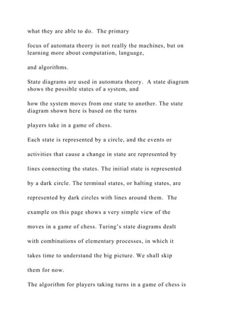
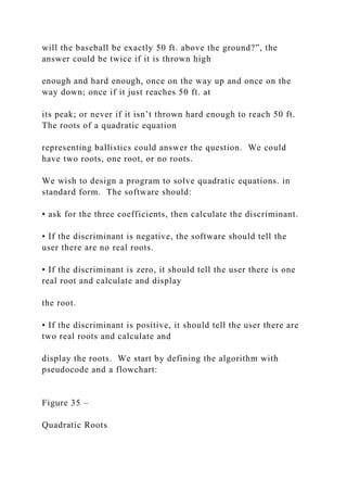
Each Unicode character has a code number. The order of the
code numbers is the order of the
characters when Unicode is used as a collating sequence. Here
is a chart showing part of the UTF-16
code1 in order. The entire UTF-16 code has over 64,000
characters (216 = 65,536) characters:
A Portion of the UTF-16 Version of Unicode
! " # $ % & ' ( ) * + - . / 0 1 2 3 4 5 6 7 8 9 : ; < = > ?
@ A B C D E F G H I J K L M N O P Q R S T U V W X Y Z [
] ^ _
` a b c d e f g h i j k l m n o p q r s t u v w x y z { | } ~
Each line in the chart is a continuation of the previous line. The
chart shows us that the numeric digits
come before uppercase letters, which come before lowercase
letters. Symbols other than alphanumeric
characters are in different parts of the code; some before
alphanumeric characters, some after.](https://image.slidesharecdn.com/anintroductiontocomputersciencewithjavapythonan-221014053824-02444449/85/An-Introduction-to-Computer-Science-with-Java-Python-an-docx-16-320.jpg)


![and discuss algorithms. We saw in
chapter 2 that pseudocode is somewhere between a human
language like English and a formal coding
language like Python or Java. It might be thought of as
structured English, which is easy to read, but
which has language structures such as [if…then…else…] and
[for count = 1 to n] to describe branching
and looping in algorithms.
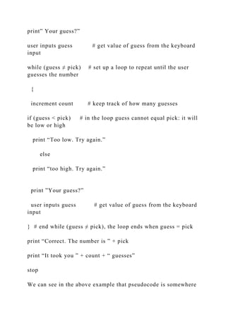
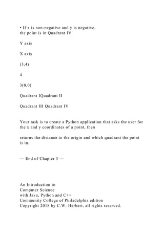
The following example describes an algorithm using both
pseudocode and a flowchart.
* * * * * * * * * * * * * * * Guessing Game Example * * * * *
* * * * * * * * * * * * * * * * * * * * * * *
We wish to create a computer program for a guessing game.
The computer will pick a random integer
between 1 and 100, and then ask the user to guess the number.
If the user’s guess is not correct, then the program should tell
the user that the guess is either too low or
too high and allow the user to guess again. This process should
continue until the user enters the
correct guess. Once the user enters the correct guess, the
computer should tell the user that the guess
is correct, along with the number of guesses it took to get the
correct number.](https://image.slidesharecdn.com/anintroductiontocomputersciencewithjavapythonan-221014053824-02444449/85/An-Introduction-to-Computer-Science-with-Java-Python-an-docx-45-320.jpg)


![Last edited September 24, 2018 by C. W. Herbert
This document is a draft of a chapter from An Introduction to
Computer Science with Java, Python and C++, written by
Charles
Herbert. It is available free of charge for students in Computer
Science courses at Community College of Philadelphia during
the
Fall 2018 semester. It may not be reproduced or distributed for
any other purposes without proper prior permission.
Please report any typos, other errors, or suggestions for
improving the text to [email protected]
Contents
Chapter 3 – Programming Logic
...............................................................................................
..................... 3
Boolean Logic in Branching and Looping
.......................................................................... 4
Boolean Relational Operations
...............................................................................................
.............. 5
Boolean Relational Operators in Python
..............................................................................................
5
Boolean Logical Operations
...............................................................................................
................... 7](https://image.slidesharecdn.com/anintroductiontocomputersciencewithjavapythonan-221014053824-02444449/85/An-Introduction-to-Computer-Science-with-Java-Python-an-docx-101-320.jpg)


![Each Unicode character has a code number. The order of the
code numbers is the order of the
characters when Unicode is used as a collating sequence. Here
is a chart showing part of the UTF-16
code1 in order. The entire UTF-16 code has over 64,000
characters (216 = 65,536) characters:
A Portion of the UTF-16 Version of Unicode
! " # $ % & ' ( ) * + - . / 0 1 2 3 4 5 6 7 8 9 : ; < = > ?
@ A B C D E F G H I J K L M N O P Q R S T U V W X Y Z [
] ^ _
` a b c d e f g h i j k l m n o p q r s t u v w x y z { | } ~
Each line in the chart is a continuation of the previous line. The
chart shows us that the numeric digits
come before uppercase letters, which come before lowercase
letters. Symbols other than alphanumeric
characters are in different parts of the code; some before
alphanumeric characters, some after.
A String value is a sequence of characters. When we learn more
about Strings, we will see that the
Unicode sequence is also used to compare String values,
character by character
Boolean Logical Operations](https://image.slidesharecdn.com/anintroductiontocomputersciencewithjavapythonan-221014053824-02444449/85/An-Introduction-to-Computer-Science-with-Java-Python-an-docx-116-320.jpg)


![Tools for Describing Algorithms
Böhm and Jacopini used a system they called flow diagrams to
describe their work. Figure 7 on page 18
is an image from their manuscript showing basic flow diagrams.
They weren’t the first to use such
diagrams, which had been around in business and industry since
the 1920s. The diagrams later became
known as flowcharts. A flow chart is a diagram showing the
logical flow and structure of an algorithm.
In CSCI 111, 112, and 211 we will see many other tools for
describing software systems in general and
algorithms in particular, such as state tables and pseudocode
like we saw above, and various UML
diagrams. For now, we will use two simple tools to illustrate the
elements of logical structure in
algorithms: simple flowcharts, similar to Böhm and Jacopini’s,
and pseudocode.
Today pseudocode is the most common tool used to describe
and discuss algorithms. We saw in
chapter 2 that pseudocode is somewhere between a human
language like English and a formal coding
language like Python or Java. It might be thought of as
structured English, which is easy to read, but
which has language structures such as [if…then…else…] and](https://image.slidesharecdn.com/anintroductiontocomputersciencewithjavapythonan-221014053824-02444449/85/An-Introduction-to-Computer-Science-with-Java-Python-an-docx-144-320.jpg)
![[for count = 1 to n] to describe branching
and looping in algorithms.
The following example describes an algorithm using both
pseudocode and a flowchart.
* * * * * * * * * * * * * * * Guessing Game Example * * * * *
* * * * * * * * * * * * * * * * * * * * * * *
We wish to create a computer program for a guessing game.
The computer will pick a random integer
between 1 and 100, and then ask the user to guess the number.
If the user’s guess is not correct, then the program should tell
the user that the guess is either too low or
too high and allow the user to guess again. This process should
continue until the user enters the
correct guess. Once the user enters the correct guess, the
computer should tell the user that the guess
is correct, along with the number of guesses it took to get the
correct number.
Here is a sample run of the program:
I am thinking of a number between 1 and 100.
Try to guess what it is.
Your guess?
50](https://image.slidesharecdn.com/anintroductiontocomputersciencewithjavapythonan-221014053824-02444449/85/An-Introduction-to-Computer-Science-with-Java-Python-an-docx-145-320.jpg)


![the
Fall 2018 semester. It may not be reproduced or distributed for
any other purposes without proper prior permission.
Please report any typos, other errors, or suggestions for
improving the text to [email protected]
Contents
Chapter 3 – Programming Logic
......................................................................................... ......
..................... 3
Boolean Logic in Branching and Looping
.......................................................................... 4
Boolean Relational Operations
...............................................................................................
.............. 5
Boolean Relational Operators in Python
..............................................................................................
5
Boolean Logical Operations
...............................................................................................
................... 7
Boolean Logical Operators in Python
...............................................................................................
... 10
Boolean Expressions Using Boolean Variables
.................................................................................... 10
CheckPoint 3.1
...............................................................................................](https://image.slidesharecdn.com/anintroductiontocomputersciencewithjavapythonan-221014053824-02444449/85/An-Introduction-to-Computer-Science-with-Java-Python-an-docx-201-320.jpg)


![A Portion of the UTF-16 Version of Unicode
! " # $ % & ' ( ) * + - . / 0 1 2 3 4 5 6 7 8 9 : ; < = > ?
@ A B C D E F G H I J K L M N O P Q R S T U V W X Y Z [
] ^ _
` a b c d e f g h i j k l m n o p q r s t u v w x y z { | } ~
Each line in the chart is a continuation of the previous line. The
chart shows us that the numeric digits
come before uppercase letters, which come before lowercase
letters. Symbols other than alphanumeric
characters are in different parts of the code; some before
alphanumeric characters, some after.
A String value is a sequence of characters. When we learn more
about Strings, we will see that the
Unicode sequence is also used to compare String values,
character by character
Boolean Logical Operations
Simple Boolean conditions based on comparing values can be
combined using Boolean logical
operations to form compound conditions, such as the burglar
alarm condition mentioned earlier:
(burglar alarm is on) AND (door is open)
There are three primary logical operations in Boolean logic:](https://image.slidesharecdn.com/anintroductiontocomputersciencewithjavapythonan-221014053824-02444449/85/An-Introduction-to-Computer-Science-with-Java-Python-an-docx-216-320.jpg)


![the 1920s. The diagrams later became
known as flowcharts. A flow chart is a diagram showing the
logical flow and structure of an algorithm.
In CSCI 111, 112, and 211 we will see many other tools for
describing software systems in general and
algorithms in particular, such as state tables and pseudocode
like we saw above, and various UML
diagrams. For now, we will use two simple tools to illustrate the
elements of logical structure in
algorithms: simple flowcharts, similar to Böhm and Jacopini’s,
and pseudocode.
Today pseudocode is the most common tool used to describe
and discuss algorithms. We saw in
chapter 2 that pseudocode is somewhere between a human
language like English and a formal coding
language like Python or Java. It might be thought of as
structured English, which is easy to read, but
which has language structures such as [if…then…else…] and
[for count = 1 to n] to describe branching
and looping in algorithms.
The following example describes an algorithm using both
pseudocode and a flowchart.
* * * * * * * * * * * * * * * Guessing Game Example * * * * *
* * * * * * * * * * * * * * * * * * * * * * *](https://image.slidesharecdn.com/anintroductiontocomputersciencewithjavapythonan-221014053824-02444449/85/An-Introduction-to-Computer-Science-with-Java-Python-an-docx-244-320.jpg)


More Related Content
Similar to An Introduction to Computer Science with Java, Python an.docx (20)
More from daniahendric (20)


Recently uploaded (20)


An Introduction to Computer Science with Java, Python an.docx
- 1. An Introduction to Computer Science with Java, Python and C++ Community College of Philadelphia edition Copyright 2018 by C.W. Herbert, all rights reserved. Last edited September 24, 2018 by C. W. Herbert This document is a draft of a chapter from An Introduction to Computer Science with Java, Python and C++, written by Charles Herbert. It is available free of charge for students in Computer Science courses at Community College of Philadelphia during the Fall 2018 semester. It may not be reproduced or distributed for any other purposes without proper prior permission. Please report any typos, other errors, or suggestions for improving the text to [email protected] Contents Chapter 3 – Programming Logic ............................................................................................... ..................... 3 Boolean Logic in Branching and Looping .......................................................................... 4 Boolean Relational Operations ............................................................................................... .............. 5
- 2. Boolean Relational Operators in Python ...................................................................................... ........ 5 Boolean Logical Operations ............................................................................................... ................... 7 Boolean Logical Operators in Python ............................................................................................... ... 10 Boolean Expressions Using Boolean Variables .................................................................................... 10 CheckPoint 3.1 ............................................................................................... ...................................... 11 The Nature of Algorithms.............................................................................. .................. 12 Turing Machines and the Church-Turing Thesis ................................................................................. 12 Elements of Logical Structure in Algorithms ....................................................................................... 16 Tools for Describing Algorithms ............................................................................................... ........... 19 Linear Sequences ...............................................................................................
- 3. ................................. 23 CheckPoint 3.2 ............................................................................................... ...................................... 24 Conditional Execution (Branching ) ................................................................................. 24 Binary Branching – Bypass vs. Choice ............................................................................................... .. 24 Binary Branching in Python ............................................................................................... .................. 25 Multiple Branching ............................................................................................... ............................... 27 Pythons elif statement ............................................................................................... ......................... 30 CheckPoint 3.3 ............................................................................................... ...................................... 31 Chapter 3 – Programming Logic DRAFT September 2018 pg. 2 Lab Reports and Collaborative Editing ............................................................................ 32
- 4. Computer Science 111 Lab Report ............................................................................................... ....... 32 Collaborative Editing of Word Documents ......................................................................................... 33 Tracking Changes ............................................................................................... ................................. 33 Document Comments ............................................................................................... .......................... 34 Lab 3A – Body Mass Index ............................................................................................... ....................... 34 Lab 3B – Quadratic Equations ............................................................................................... ................. 36 Key Terms in Chapter 3 ............................................................................................... ............................ 39 Chapter 3 – Questions ............................................................................................... ............................. 39 Chapter 3 – Exercises ............................................................................................... ............................... 40
- 5. Chapter 3 – Programming Logic DRAFT September 2018 pg. 3 Chapter 3 – Programming Logic This chapter is about branching – conditional execution of code segments that depends on the result of Boolean logic in a computer program. The chapter begins with a look at relational operations that compare values to yield true or false results, such as less than or greater than, and logical operations that combine and modify such values in Boolean expressions, such as if (hours > 40.0 and rate > 12.50). The nature of algorithms and their structure are briefly examined, including the concept of a Turing machine and its importance in the history of computer science and math. The bulk of the chapter is about branching in Python. Repetition of a code segment in an algorithm, also known as looping, will be covered in the next chapter. Learning Outcomes Upon completion of this chapter students should be able to:
- 6. • list and describe the six comparison operators and the three primary logical operators used in Boolean logic; • describe the use of comparison and relational operators in forming Python Boolean expressions; • describe the concept of a Turing machine and the nature and importance of the Church-Turing Thesis; • list and describe the three elements of logical structure in algorithms; • describe the difference between a binary bypass and a binary choice in the logic of an algorithm; • describe the concept of multiple branching and how it relates to binary branching; • describe the use of the if statement for establishing conditional execution in Python; • describe the use of the if…else statement for establishing multiple branching in Python, and how to establish nested if…else structures in Python; • describe the proper use of the elif statement for establishing multiple branching in Python. • create Python code that demonstrates correct use of each of the following: conditional
- 7. execution, multiple branching with an if…else structure, and multiple branching with an elif structure; • describe the requirements of a properly organized programming lab report for Computer Science 111, and how to use Microsoft Word’s track changes and commenting features to collaboratively edit lab reports. Chapter 3 – Programming Logic DRAFT September 2018 pg. 4 Boolean Logic in Branching and Looping In chapter one we saw Python’s Boolean data type, whose variables have the values True and False. The data type is named for George Boole, a brilliant self-taught mathematician with little formal training who became the first Professor of Mathematics at Queen’s College in Cork, Ireland. Boole wrote two books that laid a foundation for what are today known as Boolean logic and Boolean algebra: The Mathematical Analysis of Logic (1847) and An investigation into the Laws of Thought, on which are founded the Mathematical Theories of Logic and Probabilities (1854).²
- 8. The digital logic that is today the basis of both computer hardware and computer software evolved over a period of about 90 years following Boole’s first publications on the subject. Many people contributed to perfecting Boole’s ideas, in particular Augustus De Morgan at London University, London economist and mathematician William Stanley Jevons, and Claude Shannon, a Bell Labs mathematician and electrical engineer who developed digital circuit logic. Boolean logic is a system of logic dealing with operations on the values 1 and 0, in which 1 can represent true and 0 can represent false. We will use the values true and false in discussing Boolean operations. Boolean algebra is a formal language for describing operations on true and false values based on Boolean logic. Boolean algebra is covered in Math 121, Math 163 and several other courses at Community College of Philadelphia. Computers derive Boolean true and false values primarily by comparing things. For example, a condition in a payroll program might compare the number of hours a person worked to the value 40 to see if the person should receive overtime pay:
- 9. if (hours are greater than 40) calculate overtime pay The condition (hours are greater than 40) will be true or false. If it is true, then the computer will be directed to calculate overtime pay, if it is false, the computer will ignore this directive. Simple conditions such as these can be combined or modified using logical operations to form compound conditions, such as: if ((burglar alarm is on) AND (door is open)) sound alarm There are two simple conditions in this case that both need to be true for the alarm to sound. In this section we will look at the comparisons that yield true and false results and the language for specifying them in Python. In the next section, we will look at logical operations like the AND operation that form compound conditions, then see how Boolean logic forms branching and looping sequences in the structures of algorithms.
- 10. Chapter 3 – Programming Logic DRAFT September 2018 pg. 5 Boolean Relational Operations In Python programming, a Boolean variable is assigned a true or false value by using the Boolean constants True or False, or by using an assignment statement with Boolean expressions: A Boolean variable can be set to True or False, such as in the following: licensed = False citizen = True The terms True and False are known as Boolean constants or Boolean literals. Boolean literals are tokens that represent the values true and false in Python code. They are not Strings. There are only two Boolean literals – True and False. We can also obtain a true or false value by using relational operations in Boolean expressions. A relation operation is a comparison of two values to see if they are equal, or if one is greater or lesser than the other. A relational operation forms a Boolean expression that may be true or false. The
- 11. relational operations are indicated by relational operators for equality and inequality. A Boolean expression is an expression that evaluates to a true or false value. For example, the expression (x < 3) can be evaluated for a specific value of x. When x is 2, the expression evaluates to true; when x is 4, the expression evaluates to false. Boolean Relational Operators in Python There are six common relational operations in Boolean logic. The table below describes each of the six, along with the operators used for them in math and in Python programming. Boolean Relational Operations Condition math Python Examples A equals B A = B (A == B) zipcode == "19130" A is not equal to B A ≠ B (A!= B) root != 0.0 A is less than B A < B (A < B) name < "Miller" A is greater than B A > B (A > B) temperature > 98.6 A is less than or equal to B A ≤ B (A <= B) rate <= 12.50 A is greater than or equal to B A ≥ B (A >= B) bedrooms >= 3 Note that the logical operator for equals uses two equal signs
- 12. together, as opposed to the operator in Python assignment statements that uses a single equal sign. The equals and not equals operators are sometimes referred to as equality operators. The symbols for the six logical operators in Python are the same in many programming languages, including Java and C++. Simple Boolean conditions for branching in Python each have a single conditional operation in following the keyword if, as in the following example: Chapter 3 – Programming Logic DRAFT September 2018 pg. 6 if hours > 40 overtimeHours = hours - 40.0 overTimepay = overtimeHours * rate * 0.5 In this case, the condition is immediately followed by a new block of code indicated by indenting the block of code. If the condition is true, then the entire block of code will be executed. If the condition is false, the computer will skip the block of code and move on to whatever comes next in the code. This is
- 13. an example of conditional execution. We will see more about if statements in Python later in this chapter. If we compare numbers, then it is obvious what the less than and greater than operations mean, but what about text data, such as strings in Python? A collating sequence is used for comparison of text data. A collating sequence is a defined order of characters for a particular alphabet or set of symbols. The formal name for this is lexicographic order or lexicographical order A lexicon is a dictionary -- a set of words in a particular order. In mathematics, lexicographic order means that a set of word is ordered according to the defined order of their component letters. In other words, alphabetic order, according to some defined alphabet. The version of the Latin alphabet used for the English language is an example: {A, B, C, … Z}. It seems simple, but almost immediately complications can arise. What is the order of the characters if we have both uppercase and lowercase characters? Here are three different collating sequences based on the English version of the Latin alphabet with both uppercase and
- 14. lowercase characters: Three Collating Sequences for the English Alphabet 1. {A,B,C,D,E,F,G,H,I,J,K,L,M,N,O,P,Q,R,S,T,U,V,W,X,Y,Z,a,b,c ,d,e,f,g,h,i,j,k,l,m,n,o,p,q,r,s,t,u,v,w,x,y,z} 2. {a,b,c,d,e,f,g,h,i,j,k,l,m,n,o,p,q,r,s,t,u,v,w,x,y,z,A,B,C,D,E,F,G, H,I,J,K,L,M,N,O,P,Q,R,S,T,U,V,W,X,Y,Z} 3. {A,a,B,b,C,c,D,d,E,e,F,f,G,g,H,h,I,i,J,j,K,k,L,l,M,m,N,n,O,o,P, p,Q,q,R,r,S,s,T,t,U,u,V,v,W,w,X,x,Y,y,Z,z} All three sequences use the traditional A-Z order learned by children, but differ as to how they handle upper and lower case letters. In the first sequence, uppercase letters come before lowercase letters. In the second sequence lowercase letters are first, or less than the upper case letters. The third sequence is more traditional, with the uppercase and then the lowercase version of each character coming before the uppercase and lowercase version of the next character in the A-Z sequence. (Can you see what a fourth sequence might be?) Consider the order of the words "apple" and "Ball" according to the three sequences above.
- 15. • Using the first sequence, B comes before a because uppercase B comes before lowercase a; B is less than a. In this case, Ball comes before apple. • With the second sequence, lowercase letters come before uppercase letters, so a comes before B. Here apple comes before Ball. Figure 1 – Block of code in an if statement Chapter 3 – Programming Logic DRAFT September 2018 pg. 7 • The third sequence, which is more commonly used in everyday language, indicates that both uppercase and lowercase versions of a letter come before the next letter in the sequence. In this case, apple comes before Ball. We also need to consider non-alphabetic symbols in a collating sequence for text data. Do the symbols for numeric digits come before or after letters of the alphabet? What about special symbols, such as the question mark, the dollar sign, and the ampersand? What about symbols from other alphabets? As we saw in the previous chapter, most modern computer
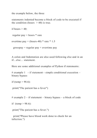
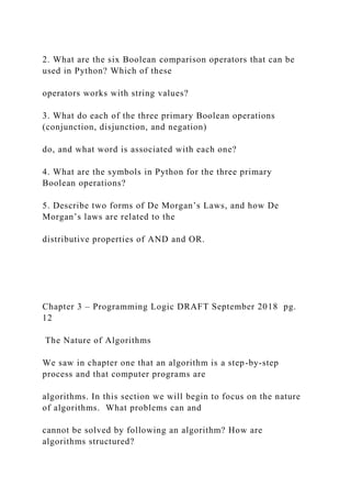
- 16. programming languages, including Python, use the defined order of the Unicode UTF-16 character set as the collating sequence for text data. So do most modern operating systems, including all current versions of Microsoft Windows, Apple OS X, and most newer Linux and Android operating systems. Each Unicode character has a code number. The order of the code numbers is the order of the characters when Unicode is used as a collating sequence. Here is a chart showing part of the UTF-16 code1 in order. The entire UTF-16 code has over 64,000 characters (216 = 65,536) characters: A Portion of the UTF-16 Version of Unicode ! " # $ % & ' ( ) * + - . / 0 1 2 3 4 5 6 7 8 9 : ; < = > ? @ A B C D E F G H I J K L M N O P Q R S T U V W X Y Z [ ] ^ _ ` a b c d e f g h i j k l m n o p q r s t u v w x y z { | } ~ Each line in the chart is a continuation of the previous line. The chart shows us that the numeric digits come before uppercase letters, which come before lowercase letters. Symbols other than alphanumeric characters are in different parts of the code; some before alphanumeric characters, some after.
- 17. A String value is a sequence of characters. When we learn more about Strings, we will see that the Unicode sequence is also used to compare String values, character by character Boolean Logical Operations Simple Boolean conditions based on comparing values can be combined using Boolean logical operations to form compound conditions, such as the burglar alarm condition mentioned earlier: (burglar alarm is on) AND (door is open) There are three primary logical operations in Boolean logic: • conjunction, represented by the word AND • disjunction, represented by the word OR • negation, represented by the word NOT The AND operator takes two Boolean operands and yields a Boolean result. If both operands are true, then the result is true, otherwise the result is false. If either operand is false, the result is false. 1 Unicode also includes characters from other languages, such as the Cyrillic, Arabic and Hebrew alphabets. For detailed information on Unicode, see the Unicode Consortium Website, online at: http://www.unicode.org/
- 18. Chapter 3 – Programming Logic DRAFT September 2018 pg. 8 The OR operator takes two Boolean operands and yields a Boolean result. If both operands are false, then the result is false, otherwise the result is true. If either operand is true, the result is true. The NOT operator is a unary operation with a single operand. If the operand is true, the result is false. If the operand is false, the result is true. This is known as inverting a Boolean value. The NOT operation inverts the true or false value of the operand. The table below defines the three primary Boolean logical operations: AND OR NOT false AND false -> false false AND true -> false true AND false -> false true AND true -> true false OR false -> false false OR true -> true
- 19. true OR false -> true true OR true -> true not(false) -> true not(true) -> false The AND and OR operations are both commutative and associative: commutative (a AND b) = (b AND a) (a OR b) = ( b OR a) associative (a AND b) AND c = a AND (b AND c) (a OR b) OR c = a OR (b OR c) AND and OR operations are not distributive with regard to the NOT operation. You may recall from elementary algebra that the distributive law involves two different operations. For example, multiplication is distributive over addition, as in these two examples: a*(b+c) = (a*b) + (a*c) 3(x+y) = 3x + 3y We often use this in reverse to simplify expressions: 17x + 11x = 28x We might be tempted to say that NOT(a AND b) = NOT(a) AND NOT(b), but this is incorrect; the NOT operation is not distributive with respect to AND, nor with respect to OR. Instead De Morgan’s laws
- 20. apply. De Morgan’s Laws NOT (a AND b) = NOT(a) OR NOT (b) NOT(a OR b) = NOT(a) AND NOT (b) Like the distributive law in elementary algebra, De Morgan’s laws are often used in reverse in computing and logic to simplify Boolean expressions. De Morgan’s laws were developed by George Boole’s contemporary, Augustus De Morgan, who, at age 22 became the first professor of Mathematics at the University of London, shortly after it was founded. In addition to the primary Boolean operations, there are derived Boolean operations, that can be derived from the three primary operations. The most common of these are NAND, NOR, and XOR. These derived Boolean operations are important in the design of modern computer chips because they are easy to mass-produce in electronic logic circuits (called gates) at a microscopic level. Some chips are composed entirely of NAND gates or of NOR gates. NAND NOR XOR a NAND b = NOT(a AND b) a NOR b = NOT(a OR b) a XOR b
- 21. = (a OR b) AND NOT(a AND b) Chapter 3 – Programming Logic DRAFT September 2018 pg. 9 Toward That Grand Prodigy: A Thinking Machine In 1984, Oxford University Press published The Boole-De Morgan Correspondence, 1842-1864, containing a collection of more than 90 letters between the two friends. George Boole in Cork and Augustus De Morgan in London laid the foundation for modern digital logic. In the Spring of 1847 Boole published Mathematical Analysis of Logic. Later that year De Morgan published Formal Logic or The Calculus of Inference. Much of modern digital electronics and computer programming is based on their work. Boole died from pneumonia in 1864 at age 49. De Morgan went on to found the field of Relational Algebra, the basis for most modern database management systems. Boole and De Morgan were part of a British circle of acquaintances important in the history of computing, including Charles Babbage and Ada Augusta Lovelace. Most of their writing is available freely online, including their books, papers, and letters.
- 22. One interesting artifact is a letter of condolence to Boole’s wife from Joseph Hill describing a meeting of Boole and Babbage at the Crystal Palace Exhibition of 1851. In it Hill wrote: … Mr. Babbage arrived and entered into a long conversation with Boole. Oh, the scene would have formed a good subject for a painter. As Boole had discovered that means of reasoning might be conducted by a mathematical process, and Babbage had invented a machine for the performance of mathematical work, the two great men together seemed to have taken steps towards the construction of that grand prodigy – a Thinking Machine.” A copy of Boole’s The Mathematical Analysis of Logic is available online at Project Guttenberg (along with his other works): http://www.gutenberg.org/ebooks/36884 De Morgan’s Formal Logic or The Calculus of Inference is at the Internet Library: https://archive.org/details/formallogicorca00morggoog A copy of Babbage’s On the Application of Machinery to the Purpose of Calculating and Printing Mathematical Tables is available online from the Hathi Trust Digital Library: http://hdl.handle.net/2027/mdp.39015004166164 Lovelace’s translation and notes from Menabrea’s Sketch of the Analytical
- 23. Engine is available in its 1843 published form at Google Books: http://books.google.com/books?id=qsY- AAAAYAAJ&pg=PA666&source=gbs_toc_r&cad=3#v=onepage &q&f=false Text from and images of Hill’s letter to MaryAnn Boole can be found online in the University of Cork’s Boole Papers Collection: http://georgeboole.ucc.ie/index.php?page=11#S01BIx George Boole 1815-1864 Augustus De Morgan 1806-1871 Charles Babbage 1791-1871 Ada Augusta Lovelace 1815-1852 http://www.gutenberg.org/ebooks/36884 https://archive.org/details/formallogicorca00morggoog http://hdl.handle.net/2027/mdp.39015004166164 http://books.google.com/books?id=qsY- AAAAYAAJ&pg=PA666&source=gbs_toc_r&cad=3#v=onepage &q&f=false http://books.google.com/books?id=qsY- AAAAYAAJ&pg=PA666&source=gbs_toc_r&cad=3#v=onepage &q&f=false http://georgeboole.ucc.ie/index.php?page=11#S01BIx Chapter 3 – Programming Logic DRAFT September 2018 pg. 10
- 24. Boolean Logical Operators in Python Compound Boolean conditions in Python are formed by using Boolean logical operations AND, OR and NOT to combine and modify simple conditions. Python simply uses the lowercase versions of the words and, or and not as the Boolean logical operators: Operation Python Notes AND op1 and op2 both operands must be True to yield True OR op1 or op2 if any operand is True the result is True NOT not(op1) the Boolean value of the operand is reversed Logical operations have an order of precedence just as numeric operations do. Parentheses may be used to group logical operations to specify an order, just as with numeric expressions. In the absence of parentheses, AND has precedence over OR. NOT modifies whatever immediately follows it. If a parenthesis follows NOT, then everything in the parentheses is resolved to a Boolean value, which is then reversed by the NOT operation. Here are examples of Boolean expressions using AND, OR, and NOT:
- 25. # more than 40 hours AND status is “hourly” # a score between 90 and 100, including 90 hours > 40 and status == “hourly” score >= 90 and score < 100 # 1,00 words or 5 pages # month not in the range 1 to 12 wordCount >1000 or pageCount > 5 month < 1 or month > 12 # not (x < 3) or not (y < 4) # not ( ( x < 3) and (y < 4) ) not(x < 3) or not(y < 4) not( x < 3 and y < 4 ) Can you see how the bottom two expressions in the examples above are related to De Morgan’s laws? Boolean Expressions Using Boolean Variables Recall that a Boolean variable has a True or False value, so a Boolean condition testing for True only needs the name of a Boolean variable, not a comparison. The statement to test if innerDoorClosed is True would be if innerDoorClosed rather than if (innerDoorClosed == true) Conversely, to test for false, the condition would be if not(innerDoorClosed) The parentheses around innerDoorClosed optional. not applies
- 26. to whatever immediately follows it. Parentheses are often used, even when not needed, for clarity. Figure 2 – compound Boolean expressions Chapter 3 – Programming Logic DRAFT September 2018 pg. 11 CheckPoint 3.1 1. How do computers derive Boolean values? 2. What are the six Boolean comparison operators that can be used in Python? Which of these operators works with string values? 3. What do each of the three primary Boolean operations (conjunction, disjunction, and negation) do, and what word is associated with each one? 4. What are the symbols in Python for the three primary Boolean operations? 5. Describe two forms of De Morgan’s Laws, and how De Morgan’s laws are related to the distributive properties of AND and OR.
- 27. Chapter 3 – Programming Logic DRAFT September 2018 pg. 12 The Nature of Algorithms We saw in chapter one that an algorithm is a step-by-step process and that computer programs are algorithms. In this section we will begin to focus on the nature of algorithms. What problems can and cannot be solved by following an algorithm? How are algorithms structured? Algorithms contain the steps necessary to complete a task or solve a particular problem. Algorithms are a part of everyday life. A recipe for baking a cake will have a list of all the ingredients needed for the cake and instructions for what to do with those ingredients. The recipe provides an algorithm for baking a cake. A child who learns to perform long division is learning an algorithm. A doctor can follow an algorithm to diagnose a patient’s illness. Professionals, such as engineers, architects, and accountants, use many different algorithms in the course of their work. Some algorithms are simple; some can be
- 28. quite long and complex. An algorithm to design the optimum propeller for an ocean-going vessel using The Holtrop and Mennen Method to determine a vessel's resistance to water uses techniques of matrix algebra with thousands of steps and must be run on a computer. Even though algorithms are an important part of life all around us, they are not the kind of thing that most people spend time thinking about. So, how much do we really know about the nature of algorithms? How much do we need to know? Mathematicians, engineers, and computer scientists need to know quite a bit about them, beginning with the question: What can and can’t be done by following an algorithm? Turing Machines and the Church-Turing Thesis in the 1930s a young mathematician at Cambridge University named Alan Turing was considering the question: Is there an algorithm to determine if any given problem can be solved with an algorithm? To Figure 3 – applied algorithms
- 29. Chapter 3 – Programming Logic DRAFT September 2018 pg. 13 answer his question, he came up with the concept of a simple theoretical machine that could follow any algorithm. Today we call his machine a Turing machine. One of the burning questions in mathematics In the late 1800s and early 1900s, was the decidability question: Is there a method we can use to look at any math problem and decide if the problem can be solved? To answer this question, we need a Boolean test – one with a clear yes or no answer – yes, this problem can be solved, or no, this problem can’t be solved. We need one test that works for all problems. Some of the best mathematicians of the time – people such as David Hilbert, Kurt Gödel, and Alonzo Church – worked on what Hilbert called the Entscheidungsproblem (German for decision-making problem). It turns out that Turing’s question is equivalent to the Entscheidungsproblem. The truth of mathematics and logic for all real numbers is based on first and second order predicate logic and a set of axioms, called Peano’s Axioms, after the 19th Century Italian mathematician who
- 30. described them. Hilbert and company were trying to prove that math is complete, consistent and decidable. They had trouble with the decidability part – the Entscheidungsproblem: Is there a method we can use to look at any math problem and decide if the problem can be solved? 2 Turing realized that this question was the same as what he called the Halting Problem: For all computer programs, is there a way to tell if any particular program that is running will halt, or continue to run indefinitely? He thought of his Turing machine as one of the simplest of computing machines, which can calculate what people can calculate. He thought of it as a tool to examine computation and algorithms. The work of Alan Turing, along with the work of Alonzo Church from Princeton University, surprised the world of mathematics by illuminating two important concepts in modern computer science: 1. All mechanical systems of algorithmic computation with real numbers are functionally equivalent. That is, given an infinite amount of time and an infinite amount of memory, they can compute exactly the same things. Today this is known as the Church-Turing Thesis. Church3
- 31. and Turing4, working independently of each other, released their results in the spring of 1936. At the time, Church was a Princeton University math professor; Turing was a 23 year old student who had finished his bachelor’s degree in 1934. 2. The answer to the halting problem, and hence the answer to the Entscheidungsproblem, was no, math is not decidable. (Gödel suggested the same thing a few years earlier with his Incompleteness Theorems, but his theorems themselves proved to be incomplete.) Church was working on a system to describe functional math called lambda calculus. Turing quickly realized and showed in an appendix to his paper that Church’s theorems based on lambda calculus were equivalent to his ideas based on the Turing machine; that whatever could be determined in Lambda 2 More specifically, Hilbert asked if there is an algorithm that can be used to decide if any given theorem is true. 3 Church, Alonzo, An Unsolvable Problem of Elementary Number Theory, Amer. Journal of Math., Vol. 58, No. 2. (1936) 4 Alan Turing, On computable numbers, with an application to the Entscheidungsproblem, Proc. London Math. Soc. (1937) s2-
- 32. 42 Chapter 3 – Programming Logic DRAFT September 2018 pg. 14 Calculus, or any other system of logic based on functional algorithms and Peano’s Axioms, could be determined with a Turing machine. Church’s former student, Stephen Kleene, showed the same thing. A Turing machine is a theoretical model for a very simple mechanical computer. A Turing machine has: 1. a tape broken up into separate squares, in each of which we can write a symbol. There is no limit to the length of the tape, it is infinitely long. (Turing mentions that he chose a tape as it is one-dimensional, as opposed to two dimensional sheets of paper.) 2. a read/write head for the tape. The square under the read/write head is called the current square. The symbol the machine just read from the current square is called the scanned symbol. 3. a state register, which is a memory that can store the current state of the machine. There are a finite number of possible states for the machine, listed in a state
- 33. table. 4. a state table with entries for each possible configuration of state and scanned symbol. A state table tells the machine what to do for each possible configuration (state, scanned symbol) of he system. There is a special initial state we can call the start state. The Turing machine has a machine execution cycle that works like this: • read the symbol in the current square; • lookup the configuration in the state table; • perform an operation based on the lookup; • set the new state of the machine. The process is repeated indefinitely, or until the machine reaches a final state and halts. In each operation, the machine can do one of three things - write a new symbol in the current square, erase the current square, or leave the current square alone; it then moves the tape to the left one square or to the right one square. Here is an example of a state table for a Turing machine:
- 34. Figure 4 – model Turing machine Chapter 3 – Programming Logic DRAFT September 2018 pg. 15 state scanned symbol operation* new state S1 0 R S1 S1 1 P0, R S2 S2 0 R S2 S2 1 P0,R S3 *Pn means print n; L move left, R move right. This example is only a small part of what could be a much longer state table. We program the machine by establishing a state table then giving the machine a tape with symbols on it. Turing was a pioneer in what has come to be known as automata theory. Automata theory is the study of theoretical computing machines to explore the nature and scope of computation. It involves the languages of such machines as well as how they operate and
- 35. what they are able to do. The primary focus of automata theory is not really the machines, but on learning more about computation, language, and algorithms. State diagrams are used in automata theory. A state diagram shows the possible states of a system, and how the system moves from one state to another. The state diagram shown here is based on the turns players take in a game of chess. Each state is represented by a circle, and the events or activities that cause a change in state are represented by lines connecting the states. The initial state is represented by a dark circle. The terminal states, or halting states, are represented by dark circles with lines around them. The example on this page shows a very simple view of the moves in a game of chess. Turing’s state diagrams dealt with combinations of elementary processes, in which it takes time to understand the big picture. We shall skip them for now. The algorithm for players taking turns in a game of chess is
- 36. shown in pseudocode on the next page. In the pseudocode we can see some items that are not needed in Python, such as braces to indicate the beginning and end of a block of instructions. We can also see some structured language that we have not yet learned about, such as the if and while instructions. The if statement sets up conditional execution – part of the algorithm is only executed if a certain condition is true. The while statement sets up repetition, part of the algorithm forms a loop that is repeated if a certain condition is true. The conditions are enclosed in parentheses. If you look back at Figure 5 – chess state digram Chapter 3 – Programming Logic DRAFT September 2018 pg. 16 the state diagram, you can find branches and loops there as well. For example, white’s turn, then black’s turn, then white’s turn, then black’s turn, and so on, is repeated until a checkmate or stalemate occurs.
- 37. We are looking at this from a higher-level, so we don’t see the details about board position that determine if there is a checkmate or stalemate, nor do we see how a player decides what move to make. Those algorithms would be far more detailed and require massive state tables and long pseudocode, or more likely, be broken down into many smaller parts that would each be described in separate units. Our purpose here is simply to see how tools such as state diagrams and pseudocode illustrate algorithms with the simple example of the flow of moves in a game of chess. # initialize variables set checkmate to false set stalemate to false set result to “draw” # when the board is placed in a new position, checkmate and stalemate are set, if applicable Start the game while (checkmate and stalemate are both false) {
- 38. white moves # white puts the board in a new position if (checkmate is now true) result = “White wins” if (checkmate and stalemate are both false) { black moves # black puts the board in a new position if (checkmate is now true) result = “Black wins” } # end if (checkmate and stalemate are both false) } # end while (checkmate and stalemate are both false) print result Stop the game Elements of Logical Structure in Algorithms Conditional execution and repetition form patterns in the sequential logic of algorithms. These patterns fall into categories that can be understood as elements of logical structure, which can be combined in a myriad of ways to form the algorithms we see in modern software. Programmers who are familiar with elements of logical structure can more easily create and edit computer programs. They can use
- 39. elements of logical structure like building blocks as they design and build software. Think about how this compares to a plumber or an electrician. A person who wishes to design a plumbing system for a building, such as a residential home, has a selection of existing parts from which to choose. We can see these parts in a hardware store – elbow joints, T- joints, certain kinds of valves, and so on. Despite the differences from one home to another, the plumbing systems will mostly be Figure 6 – chess pseudocode Chapter 3 – Programming Logic DRAFT September 2018 pg. 17 composed of the same parts, which we might think of as the elements of a plumbing system. The architects and plumbers who will design and build the system need to be familiar with each of the elements and how they fit together. The same thing is true for an electrical system. The electrical engineers and electricians who design and build such systems need to be familiar with the electrical parts
- 40. that are available, how they work, and how they fit together. Switches, wires, outlets, junction boxes, circuit breakers, and so on, can be thought of as the building blocks or elements of electrical systems. So it is with the logical structure of algorithms. The elements of logical structure are the building blocks we can put together to design and create algorithms. But, just what are these elements of logical structure? How many of them do we need to learn about? The answer is: surprisingly few. We don’t need hundreds or even dozens of different kinds of parts such as plumbers and electricians would need to build their systems. In 1966 an Italian computer scientist, Corrado Böhm and his student, Giuseppe Jacopini, published a paper in the Communications of the ACM showing that all algorithms are composed of three basic elements of logical structure, each one a sequence of instructions: 5 • linear sequences • selection sequences (conditional execution) • repetition sequences A more abstract equivalent of Böhm and Jacopini’s work
- 41. was contained in the work of Stephen Kleene in the 1930s, but Böhm and Jacopini’s 1966 paper captures the move toward structured programming that was happening in the 1960s and 1970s. Most modern programming languages, including Python, have branching and looping instructions based on what was happening then with languages like ALGOL, C and Pascal, whose underlying basis in sequential logic was described by Böhm and Jacopini. 5Corrado Böhm, Giuseppe Jacopini Flow diagrams, Turing machines and languages with only two formation rules, Communications of the ACM, Volume 9 Issue 5, May 1966 available online at: http://dl.acm.org/citation.cfm?id=365646 Figure 7 – Böhm and Jacopini flow diagrams http://dl.acm.org/citation.cfm?id=365646 Chapter 3 – Programming Logic DRAFT September 2018 pg. 18
- 42. (People) != (Turing Machines) Programmers must bridge the logical divide between the way computers work and the way people think. Computers are algorithmic and precise. They follow instructions step-by-step doing exactly what each instruction says to do, whereas, people are generally not algorithmic. People think heuristically. They are constantly looking for shortcuts and trying new ways to do things. They are creative and intelligent, interpreting language to see what it really means. But because of this, they often don’t follow directions very well, and are often imprecise in their use of language. People are not Turing machines. This can cause problems for programmers who must turn the heuristic logic of what people say into the algorithmic logic of a computer program. Here is an example: A boss says to a computer programmer: “Give me a list of all the people who live in
- 43. Pennsylvania and New Jersey.” What should the Boolean expression in our code look like, assuming each person can only live in one state? The expression will be part of a loop, looking at the data for each person, one at a time. If we write (state == “PA” and state == “NJ”) our list will be empty. The variable state cannot be equal to both PA and NJ at the same time. We need to write: (state == “PA” or state == “NJ”) to get one list with each person who lives in Pennsylvania or who lives in New Jersey. If state = “PA”, the condition will be true, and the person will be included in the list. If state = “NJ”, the condition will be true and the person will be included in the list. We will end up with one list with all of the people who live in Pennsylvania and all of the people who live in New Jersey. The boss is not using proper Boolean language. Yet, a programmer who understands Boolean logic will most likely understand the boss and translate the request properly. This example illustrates the difference between how people think and how computers work. It
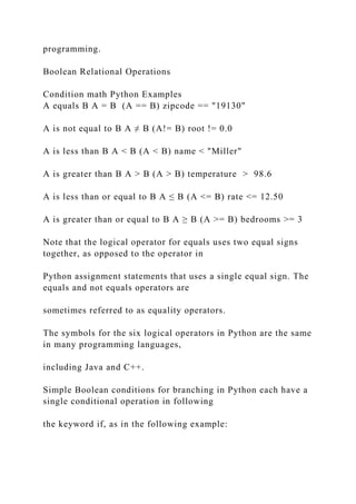
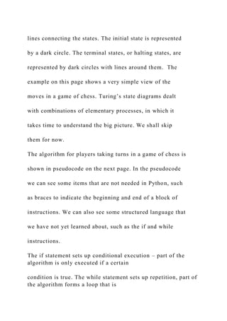
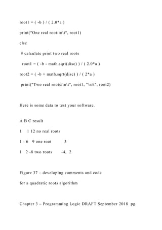
- 44. also shows that programmers are often called upon to help bridge that gap. Chapter 3 – Programming Logic DRAFT September 2018 pg. 19 Tools for Describing Algorithms Böhm and Jacopini used a system they called flow diagrams to describe their work. Figure 7 on page 18 is an image from their manuscript showing basic flow diagrams. They weren’t the first to use such diagrams, which had been around in business and industry since the 1920s. The diagrams later became known as flowcharts. A flow chart is a diagram showing the logical flow and structure of an algorithm. In CSCI 111, 112, and 211 we will see many other tools for describing software systems in general and algorithms in particular, such as state tables and pseudocode like we saw above, and various UML diagrams. For now, we will use two simple tools to illustrate the elements of logical structure in algorithms: simple flowcharts, similar to Böhm and Jacopini’s, and pseudocode. Today pseudocode is the most common tool used to describe
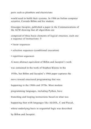
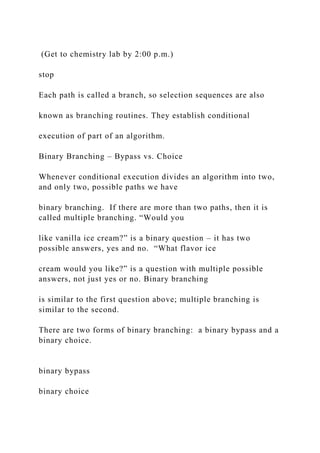
- 45. and discuss algorithms. We saw in chapter 2 that pseudocode is somewhere between a human language like English and a formal coding language like Python or Java. It might be thought of as structured English, which is easy to read, but which has language structures such as [if…then…else…] and [for count = 1 to n] to describe branching and looping in algorithms. The following example describes an algorithm using both pseudocode and a flowchart. * * * * * * * * * * * * * * * Guessing Game Example * * * * * * * * * * * * * * * * * * * * * * * * * * * * We wish to create a computer program for a guessing game. The computer will pick a random integer between 1 and 100, and then ask the user to guess the number. If the user’s guess is not correct, then the program should tell the user that the guess is either too low or too high and allow the user to guess again. This process should continue until the user enters the correct guess. Once the user enters the correct guess, the computer should tell the user that the guess is correct, along with the number of guesses it took to get the correct number.
- 46. Here is a sample run of the program: I am thinking of a number between 1 and 100. Try to guess what it is. Your guess? 50 Too low. Try again. Your guess? 75 Too High. Try Again. Your guess? 63 Too Low. Try Again. Your guess? 69 Too High. Try Again. Your guess? 66 Too High. Try Again.
- 47. Your guess? 65 Too High. Try Again. Your guess? 64 Correct! The number is 64 It took you 7 guesses The psuedocode for the algorithm is shown on the next page: Chapter 3 – Programming Logic DRAFT September 2018 pg. 20 start int pick # the number the computer picks int guess = 0 # the user’s guess, initialized to zero int count = 0 # the number of guesses pick = a random number between 1 and 100 print “I am thinking of a number between 1 and 100.” print ”Try to guess what it is.”
- 48. print” Your guess?” user inputs guess # get value of guess from the keyboard input while (guess ≠ pick) # set up a loop to repeat until the user guesses the number { increment count # keep track of how many guesses if (guess < pick) # in the loop guess cannot equal pick: it will be low or high print “Too low. Try again.” else print “too high. Try again.” print ”Your guess?” user inputs guess # get value of guess from the keyboard input } # end while (guess ≠ pick), the loop ends when guess = pick print “Correct. The number is ” + pick print “It took you ” + count + “ guesses” stop We can see in the above example that pseudocode is somewhere
- 49. between English and a programming language. Quoting from the book Introduction to Algorithms by Cormen, Lierson and Rivest: 6 “What separates pseudocode from ‘real’ code is that in pseudocode, we employ whatever expressive method is most clear and concise to specify a given algorithm. Sometimes the clearest method is English, so don’t be surprised if you come across an English expression or phrase embedded within a section of ‘real’ code. Another difference between pseudocode and real code is that pseudocode is not typically concerned with issues of software engineering. Issues of data abstraction, modularity, and error handling are often ignored in order to convey the essence of the algorithm more concisely.” 6 Cormen, Thomas; Lierson, Charles; and Rivest, Ronald; An Introduction to Algorithms; MIT Press; 1990 pg. 2 This text is an important work on algorithms, used in many advanced courses in algorithms. Figure 8 – guessing game pseudocode
- 50. Chapter 3 – Programming Logic DRAFT September 2018 pg. 21 Pseudocode often uses mixed terminology – language from both the problem domain and the implementation domain. The problem domain is the environment in which the need for software arises, such as a specific business or engineering environment. It is the world of the user of an application. The implementation domain for software is the programming environment. Pseudocode is developed as we move from specifications in the problem domain to code in the implementation domain. We need to watch for terms from the problem domain that have specialized meaning, perhaps working with an expert on the problem domain or a specially trained systems analyst to clarify language. Pseudocode uses programming terms from the implementation domain, such as if…else and while, that have a specific meaning for people with knowledge of structured programming languages, such as C, C++, Java, and Python. Terms such as if, while, and for, generally are used the same way in pseudocode as in these languages. We will use such terms as they are defined in Python, but with less formal syntax.
- 51. As we learn about conditional execution and repetition in Python, we will be learning terminology needed to understand pseudocode. The flowchart for the same algorithm as the pseudocode in Figure 8 is shown here: A flowchart may appear to be more formal and precise than pseudocode, but looks can be deceiving. Details about such things as initializing variables, how variables are used in conditions, how messages Figure 9 – guessing game flowchart Chapter 3 – Programming Logic DRAFT September 2018 pg. 22 are displayed, and so on, often are not shown in a flowchart. A flowchart is a good map of the logical flow in an algorithm, illustrating branching and looping very well, but often lacking other critical details. In an attempt to rectify this, companies like IBM in the mid-to- late 20th Century introduced many additional flowchart symbols and rules. IBM actually had a 40- page manual for flowcharting with
- 52. several dozen different symbols and a series of templates to draw flowcharts by hand, like the one shown here:7. However, drawing complicated flowcharts can make programming more cumbersome, not easier. Today the use of complicated flowcharts in software development has fallen out of favor, in part because of better use of structured language and the emergence of UML. They are still used to define business processes, in accordance with ISO standards for business process management and information systems, but used far less often by programmers to describe the details of an algorithm. We will use a simple version of flowcharting to illustrate the elements of logical structure found in our algorithms. Böhm and Jacopini’s flow diagrams were very simple. They had only two symbols: rectangles to show each step in an algorithm, and diamond-shaped boxes to show what they called a logical predicative. More commonly, a logical predicative is called a predicate or a conditional. To say that one thing is predicated on another means that one thing is determined by another. In other words, there is some
- 53. condition that will determine what happens next. We will use only four symbols: rectangles and diamonds as Böhm and Jacopini did, along with a black circle marking the beginning of an algorithm and black circles with another circle around them to represent the end of an algorithm. These symbols are the same as those used in UML activity diagrams. Effectively, we are using UML activity diagrams to illustrate the logical structures found in all algorithms – linear sequences, selections sequences (branching) and repetition sequences (loops). 7 IBM flowcharting template courtesy of Walt Johnson, retired CCP professor of Computer Information Systems and former IBM Systems Engineer. Figure 10 – IBM flow chart template Chapter 3 – Programming Logic DRAFT September 2018 pg. 23 individual steps in an algorithm are shown on a flowchart using rectangles. There is one line entering each rectangle and one line exiting each rectangle to show the
- 54. flow of a sequence of instructions. A diamond is used when branching occurs, with the condition for branching clearly stated in the diamond and multiple exits from the diamond, each with labels showing which values will cause the branching routine to select that branch of the algorithm. One-way connecting lines should be vertical or horizontal only, with directional arrows (but not too many arrows). In general, since a flowchart is used to help us see the logical structure of an algorithm, we should keep it clear and concise, doing what we can to make it easy to understand. In the rest of this chapter we will briefly look at linear sequences, then focus on conditional execution – also known as branching. We will explore repetition in the next chapter. Linear Sequences The simplest element of logical structure in an algorithm is a linear sequence, in which one instruction follows another as if in a straight line. The most notable characteristic of a linear sequence is that it has no branching or looping routines – there is only one path of logic through the sequence. It does not
- 55. divide into separate paths, and nothing is repeated. On a flowchart or activity diagram, this appears just as the name suggests, as a single path of logic, which would always be executed one step after another, as shown here. Linear sequences seem simple, but programmers need to make sure that linear sequences meet the following criteria: • They should have a clear starting and ending point. • Entry and exit conditions need to be clearly stated. What conditions need to exist before the sequence starts? What can we expect the situation (the state of the system) to be when the sequence is finished? • The sequence of instructions needs to be complete. Programmers need to be sure not to leave out any necessary steps. (This can be harder than you might expect.) • The sequence of instructions needs to be in the proper order. • Each instruction in the sequence needs to be correct. If one step in an
- 56. algorithm is incorrect, then the whole algorithm could be incorrect. In short, linear sequences must be complete, correct, and in the proper order, with clear entry and exit conditions. Linear sequences can be identified in pseudocode by the absence of branching and looping instructions – one instruction after another with no language indicating branching or looping. The same is true in most computer programming languages. Chapter 3 – Programming Logic DRAFT September 2018 pg. 24 CheckPoint 3.2 1. What does the Church-Turing Thesis tell us? 2. What is a Turing machine and how is it related to Automata Theory? 3. List and briefly describe the three elements of logical structure in algorithms, as shown by Böhm and Jacopini. 4. What are pseudocode and flowcharts and how are they used to describe algorithms?
- 57. 5. Summarize the criteria that should be met by linear sequences in algorithms. Conditional Execution (Branching ) A selection sequence, or conditional execution, occurs whenever the path or flow of sequential logic in an algorithm splits into two or more paths. As an example of a selection sequence, consider this example of a student who has chemistry lab at 2:00 p.m. on Fridays only: start if (Today is Friday) (Get to chemistry lab by 2:00 p.m.) stop Each path is called a branch, so selection sequences are also known as branching routines. They establish conditional execution of part of an algorithm. Binary Branching – Bypass vs. Choice Whenever conditional execution divides an algorithm into two, and only two, possible paths we have binary branching. If there are more than two paths, then it is called multiple branching. “Would you
- 58. like vanilla ice cream?” is a binary question – it has two possible answers, yes and no. “What flavor ice cream would you like?” is a question with multiple possible answers, not just yes or no. Binary branching is similar to the first question above; multiple branching is similar to the second. There are two forms of binary branching: a binary bypass and a binary choice. binary bypass binary choice Chapter 3 – Programming Logic DRAFT September 2018 pg. 25 In a binary bypass, part of an algorithm is either executed or bypassed. In a binary choice, one of two parts of an algorithm is chosen. The difference between a bypass and a choice is subtle but significant. In a binary bypass, it is possible that nothing happens, whereas in a binary choice, one of the two instructions will be executed, but not both. In pseudocode, a bypass is equivalent to: IF (condition) THEN
- 59. (instruction) structure. (Note that in all of these examples a single instruction could be replaced by block of instructions.) If the condition is true, then the instruction is executed; if the instruction is not true, then the instruction is ignored, and nothing happens. The chemistry lab example above shows a binary bypass. A binary choice is equivalent to an IF (condition) THEN (instruction A) ELSE (instruction B) structure. If the condition is true, then instruction A is executed; if the instruction is not true, then instruction B is executed. Either instruction A or instruction B will be executed, but not both. One of the two is always executed, as seen in the example below. A student has Math class on Monday, Wednesday, and Friday, and History class on Tuesday and Thursday. We will assume the student only needs to consider weekdays and not weekends: start if (today is Monday, or today is Wednesday, or today is Friday) (go to math class) else
- 60. (go to history class) stop The student will always go to either Math class or History class, but not both at the same time. Binary Branching in Python The if and if … else statements set up binary branching in Python. The if statement sets up simple conditional execution, sometimes also called a binary bypass as we saw above. If the condition is true, the instruction or block of instructions following the if statement is executed; if the condition is false, the instruction or block of instructions is bypassed. The terms if and else in Python are both lowercase. The Boolean condition following if could be in parentheses, but they are not required. In Python, A colon is used after the condition in an if statement and the instruction or block of instructions to be executed are indented: if hours > 40: grossPay = regular pay + (hours-40) * rate * .5
- 61. Chapter 3 – Programming Logic DRAFT September 2018 pg. 26 Indentation is used in python to mark a block of code. all of the statement indented in an if statement will be executed an one block of code if the condition is true. In the example below, the three statements indented become a block of code to be executed if the condition (hours > 40) is true. if hours > 40: regular pay = hours * rate overtime pay = (hours-40) * rate * 1.5 grosspay = regular pay + overtime pay A colon and Indentation are also used following else and in an if…else… statement. Here are some additional examples of Python if statements: # example 1 - if statement - simple conditional execution – binary bypass if (temp > 98.6): print("The patient has a fever")
- 62. # example 2 – if statement – binary bypass – a block of code if (temp > 98.6): print("The patient has a fever.") print("Please have blood work done to check for an infection.") # end if (temp > 98.6) # example 3 – if else statement – binary choice if (temp > 98.6): print("The patient has a fever") else: print("The patient’s temperature is normal") #example 4 – if statement – binary bypass – checking a range of values if (temp > 97.0) AND (temp < 99.0): print("The patient’s temperature is in the normal range.”) #example 5 – if else statement – binary choice – two blocks of code if (temp > 98.6):
- 63. print("The patient has a fever.") print("Please have blood work done to check for an infection.") # end if (temp > 98.6) else: print("The patient’s temperature is normal.") print("Please check blood pressure and pulse.") # end else (temp > 98.6) Figure 12 – examples of binary branching Chapter 3 – Programming Logic DRAFT September 2018 pg. 27 Multiple Branching As we saw earlier, multiple branching occurs when the path of logic in an algorithm divides into many different paths based on a single condition, such as “What flavor ice cream would you like?” It is not a
- 64. true or false question, but one with many different possible answers. A flowchart showing this might look something like a pitch fork, as shown in Figure 13: A multiple branching routine is equivalent to a series of binary branching routines. Consider the ice cream question. Instead of asking the multiple branching question, “What flavor ice cream would you like?”, a series of binary questions could be asked – “Would you like vanilla ice cream?”, “Would you like chocolate ice cream?”, “Would you like strawberry ice cream?”, and so on. There are two ways to do this: as independent binary branching routines or as a set of nested binary branching routines. Independent binary branching could be an inefficient solution. Consider the following psuedocode: if (flavor = vanilla) get vanilla if (flavor = chocolate) get chocolate if (flavor = strwaberry)
- 65. get strawberry …and so on. Figure 13 – multiple branching Chapter 3 – Programming Logic DRAFT September 2018 pg. 28 If the flavor does equal vanilla, and there can be only one flavor, the if routines that follow for chocolate, strawberry, and so on, are still executed, even though we know that they will be false. A better solution is to implement a set of nested binary branching routines. If the answer to any one of these questions is yes, then the branching is complete, if not, then the algorithm moves on to the next binary selection. The flowchart and pseudocode in Figure 14 shows the same ice cream question as above, but as a series as a set of nested if… else… statements, with the second if… else… enclosed in the else portion of the first if… else… , the third nested in the else portion of the second if… else…, and so on.
- 66. start if (flavor = vanilla) get vanilla else if (flavor = chocolate) get chocolate else if (flavor = strawberry) get strawberry else if (flavor = pistachio) get pistachio else get chocolate chip deliver stop
- 67. We can see from the flowchart and pseudocode that if any one of the if conditions is true, the remaining if routines are bypassed. This is a result of the nesting. Figure 14 – nested if...else statements Chapter 3 – Programming Logic DRAFT September 2018 pg. 29 The flowchart matches the pseudocode logically and shows that as soon as there is a true condition we break out of the chain of if… else… statements. However, its arrangement doesn’t give the same clear impression of the nested if.. else… structure that the pseudocode does. The flowchart in Figure15 is logically the same, but it shows the if… else... nesting more clearly. Nested if…else… statements are preferable to a series of independent if statements, but they can become messy if there are too many choices. What would this
- 68. look like if we have 28 flavors of ice cream to choose from? Here is code similar to situation above with four choices in above in Python: Figure 15 – nested if...else statements Chapter 3 – Programming Logic DRAFT September 2018 pg. 30 if flavor = "vanilla": print("vanilla") else: if flavor = "chocolate": print("chocolate ") else: if flavor = "pistachio": print("pistachio") else: print("chocolate chip")
- 69. Notice that in the above example chocolate chip becomes a default choice. If none of the if conditions are true, chocolate chip is printed. It is often better to have a default that indicates none of the available options were chosen, as in the following: if flavor = "vanilla": print("vanilla") else: if flavor = "chocolate": print("chocolate ") else: if flavor = "pistachio": print("pistachio") else: if flavor = "chocolate chip": print("chocolate chip") else: print("Your choice was not on the menu.")
- 70. Pythons elif statement Python has a an elif statement that can be used to simplify such nested branching. An elif statement takes the place of an else clause that is immediately followed by another if statement in nested branching. Like else, elif only needs to be indented to the same level as the corresponding if statement. Here is the example from above using elif: if flavor = "vanilla": print("vanilla") elif flavor = "chocolate" : print("chocolate ") elif flavor = "pistachio": print("pistachio") elif flavor = "chocolate chip": print("chocolate chip") else: print("Your choice was not on the menu.")
- 71. Chapter 3 – Programming Logic DRAFT September 2018 pg. 31 CheckPoint 3.3 1. What is the difference between a binary bypass and a binary choice in an algorithm? 2. Show how to establish a binary bypass in Python. 3. Show how to establish a binary choice in Python. 4. Show how to use nested else clauses to establish multiple branching in Python. 5. Show how to use elif for multiple branching in Python. Chapter 3 – Programming Logic DRAFT September 2018 pg. 32 Lab Reports and Collaborative Editing Lab reports are an important part of computer programming courses. They are similar to project documentation and help you to prepare for writing project documentation, which is an important part of professional programming.
- 72. Computer Science 111 Lab Report A template for programming lab reports for Computer Science 111 is included in the files for Week 3 in Canvas. Unless directed to do something different by the assignment, a programming lab report should include the following five sections: a. Heading Include your name, course and section number, semester, and identification of the assignment. b. Assignment Analysis and Design In your own words, describe the problem including input and output. Briefly describe how you developed your code. Briefly describe what your code does and how it works – including anything different or unique or special that you did in your software. If the software is long or complicated, describe how it is organized. Include a copy of any pseudocode or other design documents you used. If you worked with anyone else, asked anyone for help, or looked anything up, then mention it here. Include proper references to source material. c. Assignment Code
- 73. Include the code for your assignment as directed by the assignment or by your instructor. In most cases, this will be a zipped copy of the source code file for your program attached to the report. You can put the report and the program all in one zipped folder. In the report, either tell the reader that the code is in an attached file or include the code. A zipped folder may contain another zipped folder. In Java, You could copy the zipped folder for a NetBeans project and your lab report into a folder for your assignment, then zip the assignment folder. Alternatively, you could copy the report into your NetBeans project’s folder before zipping it. Your instructor may have specific requirements for this. d. Assignment Testing Describe how you tested this program to verify that it runs correctly. e. Assignment Evaluation Briefly describe what you learned from this project. What things did you struggle with? What was easy? Give your opinions of the process, including what you liked about the project and any
- 74. suggestions you have for improving the project. The report does not need to be long, but it should be complete. Chapter 3 – Programming Logic DRAFT September 2018 pg. 33 Collaborative Editing of Word Documents From time to time it will be necessary to work on programming projects with other people. This happens more often than not in a professional environment. You should know how to use Document Markup and Review features in Word to markup and comment on what other people have written, and to edit your own documents that have been marked by others. The notes below are for Office 2013. There are similar features in other versions of Word. There are two things you can do to mark and edit an existing document: 1. make changes to the document with Track Changes turned on; 2. add document comments to the document. The Track Changes feature and the comment feature are both found on the Review Ribbon in Word 2013, as shown below:
- 75. These features are easy to use, as described below. Several short tutorials for tracking changes and commenting in Word are available on the Web. See the following: • from Microsoft: http://office.microsoft.com/en- us/support/results.aspx?ctags=CH010372680 • from Office consultant Shauna Kelly,: http://shaunakelly.com/word/sharing/howtrackchangesworks.ht ml • a YouTube video from a graduate student: http://www.youtube.com/watch?v=AUf-IxzXyVk Tracking Changes To use track changes, click the Track Changes button to turn the feature on. The button works like a toggle switch – each time you click the button it changes the track changes setting to either on if it is off, or off if it is on. When it is on, any changes you make in the document will show up as editor’s marks in the document. The settings to the right of the Track Changes button allows you
- 76. to see the final document with the markup, to see what the original document looked like without the markup, or to see what the final New Comment Button Track Changes switch Track Changes navigation Comment navigation Figure 25 – Track Changes in Word 2013 http://office.microsoft.com/en- us/support/results.aspx?ctags=CH010372680 http://shaunakelly.com/word/sharing/howtrackchangesworks.ht ml http://www.youtube.com/watch?v=AUf-IxzXyVk Chapter 3 – Programming Logic DRAFT September 2018 pg. 34 document looks like without the markup. You should
- 77. experiment with Track Changes in Word to get a feeling for how it works. Open an old document and experiment with the settings while making changes to the document. If someone sends you a document with changes that were made while Track Changes was on, you can change the Track Changes settings to see the document showing the markup, to see it as it originally was, or to see what the final document looks like without the markup. Starting from the beginning of your document, you can use the Track Changes navigation buttons to move through the document from one change to another, accepting or rejecting the changes. Document Comments To place comments in a document without changing the document, select the location where you want to comment or click the item you wish to comment on, then click the New Comment button on the Review pane. If someone sends you a document with comments, you can move from one comment to another or delete comments using the comment navigation buttons to the
- 78. right of the New Comment button. Just as with track changes, it is best to open an existing document and experiment with document comments. Lab 3A – Body Mass Index Here is a program that will make you popular with your friends and family. According to the Centers for Disease Control, 8 “Body Mass Index (BMI) is a number calculated from a person's weight and height. BMI is an inexpensive and easy-to-perform method of screening for weight categories that may lead to health problems.” The formula for BMI using weight in pounds and height in inches and a table showing the standard weight status categories associated with BMI ranges for adults are given here: BMI = � �� ∗ 703 � is weight in pounds � is height in inches BMI Weight Category
- 79. BMI < 18.5 underweight 18.5 ≤ BMI < 25 normal 25 ≤ BMI < 30 overweight BMI ≥ 30 obese We wish to design a program that will ask the user for height and weight and then calculate and display the person’s BMI and BMI category. STEP 1. We will start by writing the BMI formula as a valid Python assignment statement: bmi = wt / (ht * ht) * 703 STEP 2. 8 The CDC Body Mass Index Web page can be found at: http://www.cdc.gov/healthyweight/assessing/bmi http://www.cdc.gov/healthyweight/assessing/bmi Chapter 3 – Programming Logic DRAFT September 2018 pg. 35 Next, we need to write the categories in the table as Boolean expressions in Python. The first and last
- 80. conditions are okay as they appear in the table, but the two middle conditions need to be rewritten. They are ranges of values. All four would look like this as Python Boolean conditions: underweight bmi < 18.5 normal 18.5 <= bmi AND bmi < 25.0 overweight 25.0 <= bmi AND bmi < 30.0 obese bmi >= 30.0 STEP 3. What variables will we need? height; # person’s height in inches weight; # person’s weight in pounds bmi; # person’s calculated body mass index category; # the BMI category STEP 4. Now we are ready to design our algorithm and describe it using pseudocode. # Body Mass Index calculator height # person’s height in inches weight # person’s weight in pounds
- 81. bmi # person’s calculated body mass index category # the BMI category print opening message get person’s height get person’s weight # calculate BMI using CDC formula bmi = wt / (ht * ht) * 703 # determine BMI category if ( bmi < 18.5 ) category = “underweight” else if ( bmi < 25.0 ) category = “normal” else if (( bmi < 30.0 ) category = “overweight” else category = “obese”;
- 82. print results – BMI and BMI category message END Figure 28 – BMI Algorithm STEP 5 It is left for you to complete the exercise by converting this to Python code and getting the program to run as a program named bmiCalculator. Chapter 3 – Programming Logic DRAFT September 2018 pg. 36 Lab 3B – Quadratic Equations A second-degree polynomial, such as �2 + 2� − 8 = 0 has the standard form ��2 + �� + � = 0. a, b and c are the coefficients of the equation. The values for x, called the roots of the equation, can be found using the quadratic formula x = −�±√�2−4�� 2� . The term (�2 − 4��) in the quadratic formula is called the
- 83. discriminant. It could be negative, zero, or positive. This will tell us how many roots a quadratic has: • If (�2 − 4��) is negative, the equation has no real roots, since a negative number has no square root. • If (�2 − 4��) is zero, then its square root is zero, and since (–b + 0) = (–b – 0), the equation has one real root: –� 2� . • If (�2 − 4��) is positive, the equation has two real roots: x1 = −�−√�2−4�� 2� and x2 = −�+√�2−4�� 2� . A positive number has two square roots. For example, both 4 and -4 are √16. Quadratic equations could represent ballistics, such as a thrown baseball. If we ask the question “When
- 84. will the baseball be exactly 50 ft. above the ground?”, the answer could be twice if it is thrown high enough and hard enough, once on the way up and once on the way down; once if it just reaches 50 ft. at its peak; or never if it isn’t thrown hard enough to reach 50 ft. The roots of a quadratic equation representing ballistics could answer the question. We could have two roots, one root, or no roots. We wish to design a program to solve quadratic equations. in standard form. The software should: • ask for the three coefficients, then calculate the discriminant. • If the discriminant is negative, the software should tell the user there are no real roots. • If the discriminant is zero, it should tell the user there is one real root and calculate and display the root. • If the discriminant is positive, it should tell the user there are two real roots and calculate and display the roots. We start by defining the algorithm with pseudocode and a flowchart: Figure 35 – Quadratic Roots
- 85. Chapter 3 – Programming Logic DRAFT September 2018 pg. 37 Finding the Roots of a Quadratic Equation start a # coefficient of x2 b # coefficient of x c # constant term disc # the discriminant root1 # the first root or only root if there is a single root root2 # the second root get values of the coefficients a, b, and c from the user calculate the discriminant disc = �2 − 4�� if (disc < 0) # no real roots print appropriate message else if (disc = 0)
- 86. # one real root root1 = –� 2� display root1 else # two real roots root1 = −�−√�2−4�� 2� root2 = −�+√�2−4�� 2� display both roots stop Once we have pseudocode that seems to be correct, we can start to turn the pseudocode into comments and begin building our program, as shown on the next
- 87. page. Figure 36 – Quadratic Roots Algorithm Chapter 3 – Programming Logic DRAFT September 2018 pg. 38 a = 0.0 # coefficient of x2 b = 0.0 # coefficient of x c = 0.0 # constant term disc = 0.0 # the discriminant root1 = 0.0 # the first root or only root if there is a single root root2 = 0.0 # the second root # get coefficient a from the user a = float( input("Enter the value of A: ") # get coefficient b from the user b = float( input("Enter the value of B: ") # get coefficient c from the user
- 88. b = float( input("Enter the value of C: ") # calculate the discriminant disc = b*b – (4.0 * a * c) if (disc < 0.0): # print no real roots print("No real roots") elif (disc == 0.0): # calculate and print one real root root1 = ( -b ) / ( 2.0*a ) print("One real root:nt", root1) else # calculate print two real roots root1 = ( -b - math.sqrt(disc) ) / ( 2.0*a ) root2 = ( -b + math.sqrt(disc) ) / ( 2*a ) print("Two real roots:nt", root1, "nt", root2) Here is some data to test your software.
- 89. A B C result 1 1 12 no real roots 1 - 6 9 one root 3 1 2 -8 two roots -4, 2 Figure 37 – developing comments and code for a quadratic roots algorithm Chapter 3 – Programming Logic DRAFT September 2018 pg. 39 Key Terms in Chapter 3 After completing this chapter, You should be able to define each of the following key terms: AND, 8 Automata theory, 15 binary branching, 24 binary bypass, 25 binary choice, 25 Boolean algebra, 4
- 90. Boolean expression, 5 Boolean literals, 5 Boolean logic, 4 Church-Turing Thesis, 13 collating sequence, 6 conditional execution, 15 conjunction, 7 De Morgan’s laws, 8 decidability question, 13 derived Boolean operations, 8 disjunction, 7 elif, 25 else, 25 flow chart, 19 Halting Problem, 13 if, 25 implementation domain, 21 inverting , 8
- 91. lexicographic order, 6 linear sequence, 23 multiple branching, 24 NAND, 8 negation, 7 NOR, 8 NOT, 8 OR, 8 problem domain, 21 relation operation, 5 repetition, 15 state diagram, 15 state table, 14 Turing machine, 13 XOR, 8 Chapter 3 – Questions 1. What values can be used in Boolean logic? How is Boolean logic different from Boolean algebra? How
- 92. do computers derive Boolean values? How else can a Boolean variable obtain a true or false value? 2. What are the six Boolean relational operations? What operators are used for these operations in Python? How is an equality operator different from a relational operator? 3. What does Python use as a collating sequence for text data? What are some other programming languages that use the same collating sequence? Which of these operating systems use the same collating sequence: Microsoft Windows, Apple OS X, most versions of Unix, and most newer Android operating systems? What is the order of the following characters using Python’s collating sequence: a, B, A, and b? 4. What are the names of the three primary logical operations in Boolean logic, and what words are used to represent each of them? Which of these is a unary operation and what does that mean? Which operation yields a true value, given a true value and a false value? Which operation yields a false value, given a true value and a false value?
- 93. Chapter 3 – Programming Logic DRAFT September 2018 pg. 40 5. Which of the Boolean logical operations are commutative and what does that mean? Which are associative and what does that mean? Which are distributive? What are the two versions of De Morgan’s laws? What statement using the OR operation would be equivalent to saying NOT (A and B)? 6. What are three common derived Boolean operations? How are primary and derived Booelan operations important in the design and manufacture of computer chips? 7. What operators are used in Python for the three primary Boolean operations? In the absence of parentheses, which of these operations takes precedence over another? 8. Who was Alan Turing? What is a Turing machine? How is his Halting Problem related to Hilbert’s Entscheidungsproblem? 9. What is Lambda Calculus? Who developed Lambda Calculus? What does the Church-Turing Thesis tell us about the relationship between what can be calculated with a Turing machine and what can be
- 94. calculated with Lambda Calculus? 10. What is the focus of automata theory? What two things does a state diagram show us about a system? 11. Why are the elements of logical structure important in designing and creating algorithms? What are the three elements of logical structure described by Bohm and Jacopini? What tool is most commonly used today to describe and discuss algorithms? 12. What is the difference between a problem domain and an implementation domain? Language from which of these domains is used in Pseudocode? How is pseudocode related to these two domains? 13. What are the four symbols used in flowcharts in this chapter that are the same as in UML activity diagrams? What does each of them represent? 14. What criteria do programmers need to make sure linear sequences meet? How can we identify linear sequences in pseudocode and computer software? 15. What is the difference between a binary bypass and a binary choice? What statements are used in Python for each of these? Chapter 3 – Exercises
- 95. 1. Write each of the following as valid Python Boolean expressions: (Pay attention to data types.) A. length of a fish greater than or equal to 22 inches B. joint income greater than $17,400 and less than or equal to $70,700 C. name less than “Smith” D. water level greater than 5 feet and less than 14 feet E. number of students less than 36 2. Write each of each of the three derived logical operations described on page 6 – NAND, NOR, and XOR – as Python Boolean expressions using only and, or, and not. Chapter 3 – Programming Logic DRAFT September 2018 pg. 41 3. We have three variables: age, weight and height. An airbag warning sign on the sun visor in the front of a car says “Passenger must be at least 12 years old, with a weight of at least 75 pounds or a height of at least 57 inches” to sit in the front seat. Write this rule as a Boolean expression. 4. In most states in the US, a vehicle must stop at an intersection with a traffic light when the traffic light is
- 96. red, except when making a right turn, in which case the driver must pause and can then make a right turn on red if the way is clear, unless otherwise posted. At a particular intersection there is a sign that says, “No right turn on red, 6 am to 6 pm, except Saturdays and Sundays.” Write the set of rules and conditions for this intersection as an if…else statement with a single Boolean expression of the form: if (Boolean condition) right turn on red else no right turn on red 5. Which of the following does not contain a valid Boolean expression, and why? a. If (romeDistance < veniceDistance OR naplesDistance) b. If (count > 10 AND count < 20) c. While (count < 5 AND > 1) d. While (height < count OR height < 12.5) e. If (message = “Hello, World.” OR “Hello, World!”) 6. We can test for divisibility by performing a remaindering operation (the % operator in Python) on a
- 97. numeric value. If A % B is 0, then A is divisible by B. For example, (15 % 3) = 0, so 15 is divisible by 3. The rule for determining if a year is a leap year can be found at the U.S. Naval Observatory’s Website online at http://aa.usno.navy.mil/faq/docs/leap_years.php Create a Python program that asks the user for the year, determines if the year is a leap year, then gives the user the result. 7. CCP Airways has a frequent flyer program that rewards people with frequent flyer miles in different categories, as follows: • up to 10,000 miles CCP Flyer • 10,000 to 24,999 miles CCP Silver Flyer • 25,000 to 50,000 miles CCP Gold Flyer • more than 50,000 miles CCP Platinum Flyer Create a Python application that asks for the user’s number of CCP Airways frequent flyer miles, then determines and displays the user’s frequent flyer status. 8. A company determines an employee’s pay based on hours times rate, with “time and a half for
- 98. overtime”. Overtime is more than 40 hours in one week. If an employee works more than 40 hours, the gross pay is equal to the regular pay for 40 hours, plus 1.5 times the rate for overtime hours. http://aa.usno.navy.mil/faq/docs/leap_years.php Chapter 3 – Programming Logic DRAFT September 2018 pg. 42 Create a Python payroll program that prompts the user to enter the employee’s name, hours, and rate; calculate gross pay; then prints a report with the employee’s data – name, hours, rate and gross pay. 9. A university recognizes graduates with high GPA’s in different honors categories using the following cutoffs: • summa cum laude 3.8 or higher • magna cum laude 3.6 or higher, up to summa cum laude • cum laude 3.2 or higher, up to magna cum laude A 2.0 GPA is needed to graduate. Students with less than a 2.0 are not eligible for graduation. Create a Python program that asks the user to enter a student’s GPA then determines and displays the
- 99. student’s graduation status. 10. The Python math library has a function to determine the hypotenuse of a right triangle, given the two other sides of the triangle: math.hypot(a, b) returns the square root of ( a2+ b2). (See the table of math Functions in Chapter 2.) Remember, a2+ b2 = c2, where a and b are the lengths of the shorter sides in a right triangle and c is the hypotenuse. So, c = √�2 + �2. The distance from any point (x,y) in a Cartesian Coordinate system to the origin (0,0) is the hypotenuse of a right triangle with the two short sides of the triangle equal to the x and y coordinates. In the example below, the distance from the point (3,4) to origin is √32 + 42, which equals 5. The example on the right also shows us that the quadrants of a Cartesian plane are numbered I through IV, with the following properties: • If both x and y are non-negative, the point is in Quadrant I. • If x is negative and y is non-negative, the point is in Quadrant II • If x and y are both negative, the point is in Quadrant III.
- 100. • If x is non-negative and y is negative, the point is in Quadrant IV. Y axis X axis (3,4) 4 3(0,0) Quadrant IQuadrant II Quadrant III Quadrant IV Your task is to create a Python application that asks the user for the x and y coordinates of a point, then returns the distance to the origin and which quadrant the point is in. — End of Chapter 3 — An Introduction to Computer Science with Java, Python and C++ Community College of Philadelphia edition Copyright 2018 by C.W. Herbert, all rights reserved.
- 101. Last edited September 24, 2018 by C. W. Herbert This document is a draft of a chapter from An Introduction to Computer Science with Java, Python and C++, written by Charles Herbert. It is available free of charge for students in Computer Science courses at Community College of Philadelphia during the Fall 2018 semester. It may not be reproduced or distributed for any other purposes without proper prior permission. Please report any typos, other errors, or suggestions for improving the text to [email protected] Contents Chapter 3 – Programming Logic ............................................................................................... ..................... 3 Boolean Logic in Branching and Looping .......................................................................... 4 Boolean Relational Operations ............................................................................................... .............. 5 Boolean Relational Operators in Python .............................................................................................. 5 Boolean Logical Operations ............................................................................................... ................... 7
- 102. Boolean Logical Operators in Python ............................................................................................... ... 10 Boolean Expressions Using Boolean Variables .................................................................................... 10 CheckPoint 3.1 ............................................................................................... ...................................... 11 The Nature of Algorithms.......................................................................... .... .................. 12 Turing Machines and the Church-Turing Thesis ................................................................................. 12 Elements of Logical Structure in Algorithms ....................................................................................... 16 Tools for Describing Algorithms ............................................................................................... ........... 19 Linear Sequences ............................................................................................... ................................. 23 CheckPoint 3.2 ............................................................................................... ...................................... 24 Conditional Execution (Branching ) ................................................................................. 24
- 103. Binary Branching – Bypass vs. Choice ............................................................................................... .. 24 Binary Branching in Python ............................................................................................... .................. 25 Multiple Branching ............................................................................................... ............................... 27 Pythons elif statement ............................................................................................... ......................... 30 CheckPoint 3.3 ............................................................................................... ...................................... 31 Chapter 3 – Programming Logic DRAFT September 2018 pg. 2 Lab Reports and Collaborative Editing ............................................................................ 32 Computer Science 111 Lab Report ............................................................................................... ....... 32 Collaborative Editing of Word Documents ......................................................................................... 33 Tracking Changes ...............................................................................................
- 104. ................................. 33 Document Comments ............................................................................................... .......................... 34 Lab 3A – Body Mass Index ............................................................................................... ....................... 34 Lab 3B – Quadratic Equations ............................................................................................... ................. 36 Key Terms in Chapter 3 ............................................................................................... ............................ 39 Chapter 3 – Questions ............................................................................................... ............................. 39 Chapter 3 – Exercises ...................................................................................... ......... ............................... 40 Chapter 3 – Programming Logic DRAFT September 2018 pg. 3 Chapter 3 – Programming Logic This chapter is about branching – conditional execution of code segments that depends on the
- 105. result of Boolean logic in a computer program. The chapter begins with a look at relational operations that compare values to yield true or false results, such as less than or greater than, and logical operations that combine and modify such values in Boolean expressions, such as if (hours > 40.0 and rate > 12.50). The nature of algorithms and their structure are briefly examined, including the concept of a Turing machine and its importance in the history of computer science and math. The bulk of the chapter is about branching in Python. Repetition of a code segment in an algorithm, also known as looping, will be covered in the next chapter. Learning Outcomes Upon completion of this chapter students should be able to: • list and describe the six comparison operators and the three primary logical operators used in Boolean logic; • describe the use of comparison and relational operators in forming Python Boolean expressions; • describe the concept of a Turing machine and the nature and
- 106. importance of the Church-Turing Thesis; • list and describe the three elements of logical structure in algorithms; • describe the difference between a binary bypass and a binary choice in the logic of an algorithm; • describe the concept of multiple branching and how it relates to binary branching; • describe the use of the if statement for establishing conditional execution in Python; • describe the use of the if…else statement for establishing multiple branching in Python, and how to establish nested if…else structures in Python; • describe the proper use of the elif statement for establishing multiple branching in Python. • create Python code that demonstrates correct use of each of the following: conditional execution, multiple branching with an if…else structure, and multiple branching with an elif structure; • describe the requirements of a properly organized programming lab report for Computer Science 111, and how to use Microsoft Word’s track changes
- 107. and commenting features to collaboratively edit lab reports. Chapter 3 – Programming Logic DRAFT September 2018 pg. 4 Boolean Logic in Branching and Looping In chapter one we saw Python’s Boolean data type, whose variables have the values True and False. The data type is named for George Boole, a brilliant self-taught mathematician with little formal training who became the first Professor of Mathematics at Queen’s College in Cork, Ireland. Boole wrote two books that laid a foundation for what are today known as Boolean logic and Boolean algebra: The Mathematical Analysis of Logic (1847) and An investigation into the Laws of Thought, on which are founded the Mathematical Theories of Logic and Probabilities (1854).² The digital logic that is today the basis of both computer hardware and computer software evolved over a period of about 90 years following Boole’s first publications on the subject. Many people contributed to perfecting Boole’s ideas, in particular Augustus De Morgan at London University, London economist
- 108. and mathematician William Stanley Jevons, and Claude Shannon, a Bell Labs mathematician and electrical engineer who developed digital circuit logic. Boolean logic is a system of logic dealing with operations on the values 1 and 0, in which 1 can represent true and 0 can represent false. We will use the values true and false in discussing Boolean operations. Boolean algebra is a formal language for describing operations on true and false values based on Boolean logic. Boolean algebra is covered in Math 121, Math 163 and several other courses at Community College of Philadelphia. Computers derive Boolean true and false values primarily by comparing things. For example, a condition in a payroll program might compare the number of hours a person worked to the value 40 to see if the person should receive overtime pay: if (hours are greater than 40) calculate overtime pay The condition (hours are greater than 40) will be true or false. If it is true, then the computer will be directed to calculate overtime pay, if it is false, the computer
- 109. will ignore this directive. Simple conditions such as these can be combined or modified using logical operations to form compound conditions, such as: if ((burglar alarm is on) AND (door is open)) sound alarm There are two simple conditions in this case that both need to be true for the alarm to sound. In this section we will look at the comparisons that yield true and false results and the language for specifying them in Python. In the next section, we will look at logical operations like the AND operation that form compound conditions, then see how Boolean logic forms branching and looping sequences in the structures of algorithms. Chapter 3 – Programming Logic DRAFT September 2018 pg. 5 Boolean Relational Operations In Python programming, a Boolean variable is assigned a true or false value by using the Boolean
- 110. constants True or False, or by using an assignment statement with Boolean expressions: A Boolean variable can be set to True or False, such as in the following: licensed = False citizen = True The terms True and False are known as Boolean constants or Boolean literals. Boolean literals are tokens that represent the values true and false in Python code. They are not Strings. There are only two Boolean literals – True and False. We can also obtain a true or false value by using relational operations in Boolean expressions. A relation operation is a comparison of two values to see if they are equal, or if one is greater or lesser than the other. A relational operation forms a Boolean expression that may be true or false. The relational operations are indicated by relational operators for equality and inequality. A Boolean expression is an expression that evaluates to a true or false value. For example, the expression (x < 3) can be evaluated for a specific value of x. When x is 2, the
- 111. expression evaluates to true; when x is 4, the expression evaluates to false. Boolean Relational Operators in Python There are six common relational operations in Boolean logic. The table below describes each of the six, along with the operators used for them in math and in Python programming. Boolean Relational Operations Condition math Python Examples A equals B A = B (A == B) zipcode == "19130" A is not equal to B A ≠ B (A!= B) root != 0.0 A is less than B A < B (A < B) name < "Miller" A is greater than B A > B (A > B) temperature > 98.6 A is less than or equal to B A ≤ B (A <= B) rate <= 12.50 A is greater than or equal to B A ≥ B (A >= B) bedrooms >= 3 Note that the logical operator for equals uses two equal signs together, as opposed to the operator in Python assignment statements that uses a single equal sign. The equals and not equals operators are sometimes referred to as equality operators. The symbols for the six logical operators in Python are the same in many programming languages,
- 112. including Java and C++. Simple Boolean conditions for branching in Python each have a single conditional operation in following the keyword if, as in the following example: Chapter 3 – Programming Logic DRAFT September 2018 pg. 6 if hours > 40 overtimeHours = hours - 40.0 overTimepay = overtimeHours * rate * 0.5 In this case, the condition is immediately followed by a new block of code indicated by indenting the block of code. If the condition is true, then the entire block of code will be executed. If the condition is false, the computer will skip the block of code and move on to whatever comes next in the code. This is an example of conditional execution. We will see more about if statements in Python later in this chapter. If we compare numbers, then it is obvious what the less than and greater than operations mean, but
- 113. what about text data, such as strings in Python? A collating sequence is used for comparison of text data. A collating sequence is a defined order of characters for a particular alphabet or set of symbols. The formal name for this is lexicographic order or lexicographical order A lexicon is a dictionary -- a set of words in a particular order. In mathematics, lexicographic order means that a set of word is ordered according to the defined order of their component letters. In other words, alphabetic order, according to some defined alphabet. The version of the Latin alphabet used for the English language is an example: {A, B, C, … Z}. It seems simple, but almost immediately complications can arise. What is the order of the characters if we have both uppercase and lowercase characters? Here are three different collating sequences based on the English version of the Latin alphabet with both uppercase and lowercase characters: Three Collating Sequences for the English Alphabet 1. {A,B,C,D,E,F,G,H,I,J,K,L,M,N,O,P,Q,R,S,T,U,V,W,X,Y,Z,a,b,c ,d,e,f,g,h,i,j,k,l,m,n,o,p,q,r,s,t,u,v,w,x,y,z} 2.
- 114. {a,b,c,d,e,f,g,h,i,j,k,l,m,n,o,p,q,r,s,t,u,v,w,x,y,z,A,B,C,D,E,F,G, H,I,J,K,L,M,N,O,P,Q,R,S,T,U,V,W,X,Y,Z} 3. {A,a,B,b,C,c,D,d,E,e,F,f,G,g,H,h,I,i,J,j,K,k,L,l,M,m,N,n,O,o,P, p,Q,q,R,r,S,s,T,t,U,u,V,v,W,w,X,x,Y,y,Z,z} All three sequences use the traditional A-Z order learned by children, but differ as to how they handle upper and lower case letters. In the first sequence, uppercase letters come before lowercase letters. In the second sequence lowercase letters are first, or less than the upper case letters. The third sequence is more traditional, with the uppercase and then the lowercase version of each character coming before the uppercase and lowercase version of the next character in the A-Z sequence. (Can you see what a fourth sequence might be?) Consider the order of the words "apple" and "Ball" according to the three sequences above. • Using the first sequence, B comes before a because uppercase B comes before lowercase a; B is less than a. In this case, Ball comes before apple. • With the second sequence, lowercase letters come before uppercase letters, so a comes before B. Here apple comes before Ball.
- 115. Figure 1 – Block of code in an if statement Chapter 3 – Programming Logic DRAFT September 2018 pg. 7 • The third sequence, which is more commonly used in everyday language, indicates that both uppercase and lowercase versions of a letter come before the next letter in the sequence. In this case, apple comes before Ball. We also need to consider non-alphabetic symbols in a collating sequence for text data. Do the symbols for numeric digits come before or after letters of the alphabet? What about special symbols, such as the question mark, the dollar sign, and the ampersand? What about symbols from other alphabets? As we saw in the previous chapter, most modern computer programming languages, including Python, use the defined order of the Unicode UTF-16 character set as the collating sequence for text data. So do most modern operating systems, including all current versions of Microsoft Windows, Apple OS X, and most newer Linux and Android operating systems.
- 116. Each Unicode character has a code number. The order of the code numbers is the order of the characters when Unicode is used as a collating sequence. Here is a chart showing part of the UTF-16 code1 in order. The entire UTF-16 code has over 64,000 characters (216 = 65,536) characters: A Portion of the UTF-16 Version of Unicode ! " # $ % & ' ( ) * + - . / 0 1 2 3 4 5 6 7 8 9 : ; < = > ? @ A B C D E F G H I J K L M N O P Q R S T U V W X Y Z [ ] ^ _ ` a b c d e f g h i j k l m n o p q r s t u v w x y z { | } ~ Each line in the chart is a continuation of the previous line. The chart shows us that the numeric digits come before uppercase letters, which come before lowercase letters. Symbols other than alphanumeric characters are in different parts of the code; some before alphanumeric characters, some after. A String value is a sequence of characters. When we learn more about Strings, we will see that the Unicode sequence is also used to compare String values, character by character Boolean Logical Operations
- 117. Simple Boolean conditions based on comparing values can be combined using Boolean logical operations to form compound conditions, such as the burglar alarm condition mentioned earlier: (burglar alarm is on) AND (door is open) There are three primary logical operations in Boolean logic: • conjunction, represented by the word AND • disjunction, represented by the word OR • negation, represented by the word NOT The AND operator takes two Boolean operands and yields a Boolean result. If both operands are true, then the result is true, otherwise the result is false. If either operand is false, the result is false. 1 Unicode also includes characters from other languages, such as the Cyrillic, Arabic and Hebrew alphabets. For detailed information on Unicode, see the Unicode Consortium Website, online at: http://www.unicode.org/ Chapter 3 – Programming Logic DRAFT September 2018 pg. 8 The OR operator takes two Boolean operands and yields a Boolean result. If both operands are false, then the result is false, otherwise the result is true. If either
- 118. operand is true, the result is true. The NOT operator is a unary operation with a single operand. If the operand is true, the result is false. If the operand is false, the result is true. This is known as inverting a Boolean value. The NOT operation inverts the true or false value of the operand. The table below defines the three primary Boolean logical operations: AND OR NOT false AND false -> false false AND true -> false true AND false -> false true AND true -> true false OR false -> false false OR true -> true true OR false -> true true OR true -> true not(false) -> true not(true) -> false The AND and OR operations are both commutative and
- 119. associative: commutative (a AND b) = (b AND a) (a OR b) = ( b OR a) associative (a AND b) AND c = a AND (b AND c) (a OR b) OR c = a OR (b OR c) AND and OR operations are not distributive with regard to the NOT operation. You may recall from elementary algebra that the distributive law involves two different operations. For example, multiplication is distributive over addition, as in these two examples: a*(b+c) = (a*b) + (a*c) 3(x+y) = 3x + 3y We often use this in reverse to simplify expressions: 17x + 11x = 28x We might be tempted to say that NOT(a AND b) = NOT(a) AND NOT(b), but this is incorrect; the NOT operation is not distributive with respect to AND, nor with respect to OR. Instead De Morgan’s laws apply. De Morgan’s Laws NOT (a AND b) = NOT(a) OR NOT (b) NOT(a OR b) = NOT(a) AND NOT (b) Like the distributive law in elementary algebra, De Morgan’s
- 120. laws are often used in reverse in computing and logic to simplify Boolean expressions. De Morgan’s laws were developed by George Boole’s contemporary, Augustus De Morgan, who, at age 22 became the first professor of Mathematics at the University of London, shortly after it was founded. In addition to the primary Boolean operations, there are derived Boolean operations, that can be derived from the three primary operations. The most common of these are NAND, NOR, and XOR. These derived Boolean operations are important in the design of modern computer chips because they are easy to mass-produce in electronic logic circuits (called gates) at a microscopic level. Some chips are composed entirely of NAND gates or of NOR gates. NAND NOR XOR a NAND b = NOT(a AND b) a NOR b = NOT(a OR b) a XOR b = (a OR b) AND NOT(a AND b) Chapter 3 – Programming Logic DRAFT September 2018 pg. 9 Toward That Grand Prodigy: A Thinking Machine
- 121. In 1984, Oxford University Press published The Boole-De Morgan Correspondence, 1842-1864, containing a collection of more than 90 letters between the two friends. George Boole in Cork and Augustus De Morgan in London laid the foundation for modern digital logic. In the Spring of 1847 Boole published Mathematical Analysis of Logic. Later that year De Morgan published Formal Logic or The Calculus of Inference. Much of modern digital electronics and computer programming is based on their work. Boole died from pneumonia in 1864 at age 49. De Morgan went on to found the field of Relational Algebra, the basis for most modern database management systems. Boole and De Morgan were part of a British circle of acquaintances important in the history of computing, including Charles Babbage and Ada Augusta Lovelace. Most of their writing is available freely online, including their books, papers, and letters. One interesting artifact is a letter of condolence to Boole’s wife from Joseph Hill describing a meeting of Boole and Babbage at the Crystal Palace Exhibition of 1851. In it Hill wrote: … Mr. Babbage arrived and entered into a long conversation with Boole. Oh, the scene
- 122. would have formed a good subject for a painter. As Boole had discovered that means of reasoning might be conducted by a mathematical process, and Babbage had invented a machine for the performance of mathematical work, the two great men together seemed to have taken steps towards the construction of that grand prodigy – a Thinking Machine.” A copy of Boole’s The Mathematical Analysis of Logic is available online at Project Guttenberg (along with his other works): http://www.gutenberg.org/ebooks/36884 De Morgan’s Formal Logic or The Calculus of Inference is at the Internet Library: https://archive.org/details/formallogicorca00morggoog A copy of Babbage’s On the Application of Machinery to the Purpose of Calculating and Printing Mathematical Tables is available online from the Hathi Trust Digital Library: http://hdl.handle.net/2027/mdp.39015004166164 Lovelace’s translation and notes from Menabrea’s Sketch of the Analytical Engine is available in its 1843 published form at Google Books: http://books.google.com/books?id=qsY- AAAAYAAJ&pg=PA666&source=gbs_toc_r&cad=3#v=onepage &q&f=false Text from and images of Hill’s letter to MaryAnn Boole can be found online in the University of Cork’s Boole Papers Collection: http://georgeboole.ucc.ie/index.php?page=11#S01BIx
- 123. George Boole 1815-1864 Augustus De Morgan 1806-1871 Charles Babbage 1791-1871 Ada Augusta Lovelace 1815-1852 http://www.gutenberg.org/ebooks/36884 https://archive.org/details/formallogicorca00morggoog http://hdl.handle.net/2027/mdp.39015004166164 http://books.google.com/books?id=qsY- AAAAYAAJ&pg=PA666&source=gbs_toc_r&cad=3#v=onepage &q&f=false http://books.google.com/books?id=qsY- AAAAYAAJ&pg=PA666&source=gbs_toc_r&cad=3#v=onepage &q&f=false http://georgeboole.ucc.ie/index.php?page=11#S01BIx Chapter 3 – Programming Logic DRAFT September 2018 pg. 10 Boolean Logical Operators in Python Compound Boolean conditions in Python are formed by using Boolean logical operations AND, OR and NOT to combine and modify simple conditions. Python simply uses the lowercase versions of the words
- 124. and, or and not as the Boolean logical operators: Operation Python Notes AND op1 and op2 both operands must be True to yield True OR op1 or op2 if any operand is True the result is True NOT not(op1) the Boolean value of the operand is reversed Logical operations have an order of precedence just as numeric operations do. Parentheses may be used to group logical operations to specify an order, just as with numeric expressions. In the absence of parentheses, AND has precedence over OR. NOT modifies whatever immediately follows it. If a parenthesis follows NOT, then everything in the parentheses is resolved to a Boolean value, which is then reversed by the NOT operation. Here are examples of Boolean expressions using AND, OR, and NOT: # more than 40 hours AND status is “hourly” # a score between 90 and 100, including 90 hours > 40 and status == “hourly” score >= 90 and score < 100 # 1,00 words or 5 pages # month not in the range 1 to 12 wordCount >1000 or pageCount > 5 month < 1 or month > 12
- 125. # not (x < 3) or not (y < 4) # not ( ( x < 3) and (y < 4) ) not(x < 3) or not(y < 4) not( x < 3 and y < 4 ) Can you see how the bottom two expressions in the examples above are related to De Morgan’s laws? Boolean Expressions Using Boolean Variables Recall that a Boolean variable has a True or False value, so a Boolean condition testing for True only needs the name of a Boolean variable, not a comparison. The statement to test if innerDoorClosed is True would be if innerDoorClosed rather than if (innerDoorClosed == true) Conversely, to test for false, the condition would be if not(innerDoorClosed) The parentheses around innerDoorClosed optional. not applies to whatever immediately follows it. Parentheses are often used, even when not needed, for clarity. Figure 2 – compound Boolean expressions
- 126. Chapter 3 – Programming Logic DRAFT September 2018 pg. 11 CheckPoint 3.1 1. How do computers derive Boolean values? 2. What are the six Boolean comparison operators that can be used in Python? Which of these operators works with string values? 3. What do each of the three primary Boolean operations (conjunction, disjunction, and negation) do, and what word is associated with each one? 4. What are the symbols in Python for the three primary Boolean operations? 5. Describe two forms of De Morgan’s Laws, and how De Morgan’s laws are related to the distributive properties of AND and OR. Chapter 3 – Programming Logic DRAFT September 2018 pg. 12 The Nature of Algorithms
- 127. We saw in chapter one that an algorithm is a step-by-step process and that computer programs are algorithms. In this section we will begin to focus on the nature of algorithms. What problems can and cannot be solved by following an algorithm? How are algorithms structured? Algorithms contain the steps necessary to complete a task or solve a particular problem. Algorithms are a part of everyday life. A recipe for baking a cake will have a list of all the ingredients needed for the cake and instructions for what to do with those ingredients. The recipe provides an algorithm for baking a cake. A child who learns to perform long division is learning an algorithm. A doctor can follow an algorithm to diagnose a patient’s illness. Professionals, such as engineers, architects, and accountants, use many different algorithms in the course of their work. Some algorithms are simple; some can be quite long and complex. An algorithm to design the optimum propeller for an ocean-going vessel using The Holtrop and Mennen Method to determine a vessel's resistance to water uses techniques of matrix algebra with thousands of steps and must be run on a computer.
- 128. Even though algorithms are an important part of life all around us, they are not the kind of thing that most people spend time thinking about. So, how much do we really know about the nature of algorithms? How much do we need to know? Mathematicians, engineers, and computer scientists need to know quite a bit about them, beginning with the question: What can and can’t be done by following an algorithm? Turing Machines and the Church-Turing Thesis in the 1930s a young mathematician at Cambridge University named Alan Turing was considering the question: Is there an algorithm to determine if any given problem can be solved with an algorithm? To Figure 3 – applied algorithms Chapter 3 – Programming Logic DRAFT September 2018 pg. 13 answer his question, he came up with the concept of a simple theoretical machine that could follow any algorithm. Today we call his machine a Turing machine.
- 129. One of the burning questions in mathematics In the late 1800s and early 1900s, was the decidability question: Is there a method we can use to look at any math problem and decide if the problem can be solved? To answer this question, we need a Boolean test – one with a clear yes or no answer – yes, this problem can be solved, or no, this problem can’t be solved. We need one test that works for all problems. Some of the best mathematicians of the time – people such as David Hilbert, Kurt Gödel, and Alonzo Church – worked on what Hilbert called the Entscheidungsproblem (German for decision-making problem). It turns out that Turing’s question is equivalent to the Entscheidungsproblem. The truth of mathematics and logic for all real numbers is based on first and second order predicate logic and a set of axioms, called Peano’s Axioms, after the 19th Century Italian mathematician who described them. Hilbert and company were trying to prove that math is complete, consistent and decidable. They had trouble with the decidability part – the Entscheidungsproblem: Is there a method we can use to look at any math problem and decide if the problem can be solved? 2
- 130. Turing realized that this question was the same as what he called the Halting Problem: For all computer programs, is there a way to tell if any particular program that is running will halt, or continue to run indefinitely? He thought of his Turing machine as one of the simplest of computing machines, which can calculate what people can calculate. He thought of it as a tool to examine computation and algorithms. The work of Alan Turing, along with the work of Alonzo Church from Princeton University, surprised the world of mathematics by illuminating two important concepts in modern computer science: 1. All mechanical systems of algorithmic computation with real numbers are functionally equivalent. That is, given an infinite amount of time and an infinite amount of memory, they can compute exactly the same things. Today this is known as the Church-Turing Thesis. Church3 and Turing4, working independently of each other, released their results in the spring of 1936. At the time, Church was a Princeton University math professor; Turing was a 23 year old student who had finished his bachelor’s degree in 1934.
- 131. 2. The answer to the halting problem, and hence the answer to the Entscheidungsproblem, was no, math is not decidable. (Gödel suggested the same thing a few years earlier with his Incompleteness Theorems, but his theorems themselves proved to be incomplete.) Church was working on a system to describe functional math called lambda calculus. Turing quickly realized and showed in an appendix to his paper that Church’s theorems based on lambda calculus were equivalent to his ideas based on the Turing machine; that whatever could be determined in Lambda 2 More specifically, Hilbert asked if there is an algorithm that can be used to decide if any given theorem is true. 3 Church, Alonzo, An Unsolvable Problem of Elementary Number Theory, Amer. Journal of Math., Vol. 58, No. 2. (1936) 4 Alan Turing, On computable numbers, with an application to the Entscheidungsproblem, Proc. London Math. Soc. (1937) s2- 42 Chapter 3 – Programming Logic DRAFT September 2018 pg. 14 Calculus, or any other system of logic based on functional algorithms and Peano’s Axioms, could be
- 132. determined with a Turing machine. Church’s former student, Stephen Kleene, showed the same thing. A Turing machine is a theoretical model for a very simple mechanical computer. A Turing machine has: 1. a tape broken up into separate squares, in each of which we can write a symbol. There is no limit to the length of the tape, it is infinitely long. (Turing mentions that he chose a tape as it is one-dimensional, as opposed to two dimensional sheets of paper.) 2. a read/write head for the tape. The square under the read/write head is called the current square. The symbol the machine just read from the current square is called the scanned symbol. 3. a state register, which is a memory that can store the current state of the machine. There are a finite number of possible states for the machine, listed in a state table. 4. a state table with entries for each possible configuration of state and scanned symbol. A state table tells the machine what to do for each possible configuration (state, scanned symbol) of he system. There is a special initial state we can call the start
- 133. state. The Turing machine has a machine execution cycle that works like this: • read the symbol in the current square; • lookup the configuration in the state table; • perform an operation based on the lookup; • set the new state of the machine. The process is repeated indefinitely, or until the machine reaches a final state and halts. In each operation, the machine can do one of three things - write a new symbol in the current square, erase the current square, or leave the current square alone; it then moves the tape to the left one square or to the right one square. Here is an example of a state table for a Turing machine: Figure 4 – model Turing machine Chapter 3 – Programming Logic DRAFT September 2018 pg. 15
- 134. state scanned symbol operation* new state S1 0 R S1 S1 1 P0, R S2 S2 0 R S2 S2 1 P0,R S3 *Pn means print n; L move left, R move right. This example is only a small part of what could be a much longer state table. We program the machine by establishing a state table then giving the machine a tape with symbols on it. Turing was a pioneer in what has come to be known as automata theory. Automata theory is the study of theoretical computing machines to explore the nature and scope of computation. It involves the languages of such machines as well as how they operate and what they are able to do. The primary focus of automata theory is not really the machines, but on learning more about computation, language, and algorithms. State diagrams are used in automata theory. A state diagram shows the possible states of a system, and
- 135. how the system moves from one state to another. The state diagram shown here is based on the turns players take in a game of chess. Each state is represented by a circle, and the events or activities that cause a change in state are represented by lines connecting the states. The initial state is represented by a dark circle. The terminal states, or halting states, are represented by dark circles with lines around them. The example on this page shows a very simple view of the moves in a game of chess. Turing’s state diagrams dealt with combinations of elementary processes, in which it takes time to understand the big picture. We shall skip them for now. The algorithm for players taking turns in a game of chess is shown in pseudocode on the next page. In the pseudocode we can see some items that are not needed in Python, such as braces to indicate the beginning and end of a block of instructions. We can also see some structured language that
- 136. we have not yet learned about, such as the if and while instructions. The if statement sets up conditional execution – part of the algorithm is only executed if a certain condition is true. The while statement sets up repetition, part of the algorithm forms a loop that is repeated if a certain condition is true. The conditions are enclosed in parentheses. If you look back at Figure 5 – chess state digram Chapter 3 – Programming Logic DRAFT September 2018 pg. 16 the state diagram, you can find branches and loops there as well. For example, white’s turn, then black’s turn, then white’s turn, then black’s turn, and so on, is repeated until a checkmate or stalemate occurs. We are looking at this from a higher-level, so we don’t see the details about board position that determine if there is a checkmate or stalemate, nor do we see how a player decides what move to make. Those algorithms would be far more detailed and require massive state tables and long
- 137. pseudocode, or more likely, be broken down into many smaller parts that would each be described in separate units. Our purpose here is simply to see how tools such as state diagrams and pseudocode illustrate algorithms with the simple example of the flow of moves in a game of chess. # initialize variables set checkmate to false set stalemate to false set result to “draw” # when the board is placed in a new position, checkmate and stalemate are set, if applicable Start the game while (checkmate and stalemate are both false) { white moves # white puts the board in a new position if (checkmate is now true) result = “White wins” if (checkmate and stalemate are both false) { black moves # black puts the board in a new position
- 138. if (checkmate is now true) result = “Black wins” } # end if (checkmate and stalemate are both false) } # end while (checkmate and stalemate are both false) print result Stop the game Elements of Logical Structure in Algorithms Conditional execution and repetition form patterns in the sequential logic of algorithms. These patterns fall into categories that can be understood as elements of logical structure, which can be combined in a myriad of ways to form the algorithms we see in modern software. Programmers who are familiar with elements of logical structure can more easily create and edit computer programs. They can use elements of logical structure like building blocks as they design and build software. Think about how this compares to a plumber or an electrician. A person who wishes to design a plumbing system for a building, such as a residential home, has a selection of existing parts from which
- 139. to choose. We can see these parts in a hardware store – elbow joints, T- joints, certain kinds of valves, and so on. Despite the differences from one home to another, the plumbing systems will mostly be Figure 6 – chess pseudocode Chapter 3 – Programming Logic DRAFT September 2018 pg. 17 composed of the same parts, which we might think of as the elements of a plumbing system. The architects and plumbers who will design and build the system need to be familiar with each of the elements and how they fit together. The same thing is true for an electrical system. The electrical engineers and electricians who design and build such systems need to be familiar with the electrical parts that are available, how they work, and how they fit together. Switches, wires, outlets, junction boxes, circuit breakers, and so on, can be thought of as the building blocks or elements of electrical systems. So it is with the logical structure of algorithms. The elements
- 140. of logical structure are the building blocks we can put together to design and create algorithms. But, just what are these elements of logical structure? How many of them do we need to learn about? The answer is: surprisingly few. We don’t need hundreds or even dozens of different kinds of parts such as plumbers and electricians would need to build their systems. In 1966 an Italian computer scientist, Corrado Böhm and his student, Giuseppe Jacopini, published a paper in the Communications of the ACM showing that all algorithms are composed of three basic elements of logical structure, each one a sequence of instructions: 5 • linear sequences • selection sequences (conditional execution) • repetition sequences A more abstract equivalent of Böhm and Jacopini’s work was contained in the work of Stephen Kleene in the 1930s, but Böhm and Jacopini’s 1966 paper captures the move toward structured programming that was happening in the 1960s and 1970s. Most modern
- 141. programming languages, including Python, have branching and looping instructions based on what was happening then with languages like ALGOL, C and Pascal, whose underlying basis in sequential logic was described by Böhm and Jacopini. 5Corrado Böhm, Giuseppe Jacopini Flow diagrams, Turing machines and languages with only two formation rules, Communications of the ACM, Volume 9 Issue 5, May 1966 available online at: http://dl.acm.org/citation.cfm?id=365646 Figure 7 – Böhm and Jacopini flow diagrams http://dl.acm.org/citation.cfm?id=365646 Chapter 3 – Programming Logic DRAFT September 2018 pg. 18 (People) != (Turing Machines) Programmers must bridge the logical divide between the way computers work and the way people think. Computers are algorithmic and precise. They follow instructions step-by-step
- 142. doing exactly what each instruction says to do, whereas, people are generally not algorithmic. People think heuristically. They are constantly looking for shortcuts and trying new ways to do things. They are creative and intelligent, interpreting language to see what it really means. But because of this, they often don’t follow directions very well, and are often imprecise in their use of language. People are not Turing machines. This can cause problems for programmers who must turn the heuristic logic of what people say into the algorithmic logic of a computer program. Here is an example: A boss says to a computer programmer: “Give me a list of all the people who live in Pennsylvania and New Jersey.” What should the Boolean expression in our code look like, assuming each person can only live in one state? The expression will be part of a loop, looking at the data for each person, one at a time. If we write (state == “PA” and state == “NJ”) our list will be
- 143. empty. The variable state cannot be equal to both PA and NJ at the same time. We need to write: (state == “PA” or state == “NJ”) to get one list with each person who lives in Pennsylvania or who lives in New Jersey. If state = “PA”, the condition will be true, and the person will be included in the list. If state = “NJ”, the condition will be true and the person will be included in the list. We will end up with one list with all of the people who live in Pennsylvania and all of the people who live in New Jersey. The boss is not using proper Boolean language. Yet, a programmer who understands Boolean logic will most likely understand the boss and translate the request properly. This example illustrates the difference between how people think and how computers work. It also shows that programmers are often called upon to help bridge that gap. Chapter 3 – Programming Logic DRAFT September 2018 pg. 19
- 144. Tools for Describing Algorithms Böhm and Jacopini used a system they called flow diagrams to describe their work. Figure 7 on page 18 is an image from their manuscript showing basic flow diagrams. They weren’t the first to use such diagrams, which had been around in business and industry since the 1920s. The diagrams later became known as flowcharts. A flow chart is a diagram showing the logical flow and structure of an algorithm. In CSCI 111, 112, and 211 we will see many other tools for describing software systems in general and algorithms in particular, such as state tables and pseudocode like we saw above, and various UML diagrams. For now, we will use two simple tools to illustrate the elements of logical structure in algorithms: simple flowcharts, similar to Böhm and Jacopini’s, and pseudocode. Today pseudocode is the most common tool used to describe and discuss algorithms. We saw in chapter 2 that pseudocode is somewhere between a human language like English and a formal coding language like Python or Java. It might be thought of as structured English, which is easy to read, but which has language structures such as [if…then…else…] and
- 145. [for count = 1 to n] to describe branching and looping in algorithms. The following example describes an algorithm using both pseudocode and a flowchart. * * * * * * * * * * * * * * * Guessing Game Example * * * * * * * * * * * * * * * * * * * * * * * * * * * * We wish to create a computer program for a guessing game. The computer will pick a random integer between 1 and 100, and then ask the user to guess the number. If the user’s guess is not correct, then the program should tell the user that the guess is either too low or too high and allow the user to guess again. This process should continue until the user enters the correct guess. Once the user enters the correct guess, the computer should tell the user that the guess is correct, along with the number of guesses it took to get the correct number. Here is a sample run of the program: I am thinking of a number between 1 and 100. Try to guess what it is. Your guess? 50
- 146. Too low. Try again. Your guess? 75 Too High. Try Again. Your guess? 63 Too Low. Try Again. Your guess? 69 Too High. Try Again. Your guess? 66 Too High. Try Again. Your guess? 65 Too High. Try Again. Your guess? 64
- 147. Correct! The number is 64 It took you 7 guesses The psuedocode for the algorithm is shown on the next page: Chapter 3 – Programming Logic DRAFT September 2018 pg. 20 start int pick # the number the computer picks int guess = 0 # the user’s guess, initialized to zero int count = 0 # the number of guesses pick = a random number between 1 and 100 print “I am thinking of a number between 1 and 100.” print ”Try to guess what it is.” print” Your guess?” user inputs guess # get value of guess from the keyboard input while (guess ≠ pick) # set up a loop to repeat until the user guesses the number {
- 148. increment count # keep track of how many guesses if (guess < pick) # in the loop guess cannot equal pick: it will be low or high print “Too low. Try again.” else print “too high. Try again.” print ”Your guess?” user inputs guess # get value of guess from the keyboard input } # end while (guess ≠ pick), the loop ends when guess = pick print “Correct. The number is ” + pick print “It took you ” + count + “ guesses” stop We can see in the above example that pseudocode is somewhere between English and a programming language. Quoting from the book Introduction to Algorithms by Cormen, Lierson and Rivest: 6 “What separates pseudocode from ‘real’ code is that in pseudocode, we employ whatever expressive method is most clear and concise to specify a given
- 149. algorithm. Sometimes the clearest method is English, so don’t be surprised if you come across an English expression or phrase embedded within a section of ‘real’ code. Another difference between pseudocode and real code is that pseudocode is not typically concerned with issues of software engineering. Issues of data abstraction, modularity, and error handling are often ignored in order to convey the essence of the algorithm more concisely.” 6 Cormen, Thomas; Lierson, Charles; and Rivest, Ronald; An Introduction to Algorithms; MIT Press; 1990 pg. 2 This text is an important work on algorithms, used in many advanced courses in algorithms. Figure 8 – guessing game pseudocode Chapter 3 – Programming Logic DRAFT September 2018 pg. 21 Pseudocode often uses mixed terminology – language from both the problem domain and the implementation domain. The problem domain is the environment in which the need for software arises,
- 150. such as a specific business or engineering environment. It is the world of the user of an application. The implementation domain for software is the programming environment. Pseudocode is developed as we move from specifications in the problem domain to code in the implementation domain. We need to watch for terms from the problem domain that have specialized meaning, perhaps working with an expert on the problem domain or a specially trained systems analyst to clarify language. Pseudocode uses programming terms from the implementation domain, such as if…else and while, that have a specific meaning for people with knowledge of structured programming languages, such as C, C++, Java, and Python. Terms such as if, while, and for, generally are used the same way in pseudocode as in these languages. We will use such terms as they are defined in Python, but with less formal syntax. As we learn about conditional execution and repetition in Python, we will be learning terminology needed to understand pseudocode. The flowchart for the same algorithm as the pseudocode in Figure 8 is shown here:
- 151. A flowchart may appear to be more formal and precise than pseudocode, but looks can be deceiving. Details about such things as initializing variables, how variables are used in conditions, how messages Figure 9 – guessing game flowchart Chapter 3 – Programming Logic DRAFT September 2018 pg. 22 are displayed, and so on, often are not shown in a flowchart. A flowchart is a good map of the logical flow in an algorithm, illustrating branching and looping very well, but often lacking other critical details. In an attempt to rectify this, companies like IBM in the mid-to- late 20th Century introduced many additional flowchart symbols and rules. IBM actually had a 40- page manual for flowcharting with several dozen different symbols and a series of templates to draw flowcharts by hand, like the one shown here:7. However, drawing complicated flowcharts can make programming more cumbersome, not easier.
- 152. Today the use of complicated flowcharts in software development has fallen out of favor, in part because of better use of structured language and the emergence of UML. They are still used to define business processes, in accordance with ISO standards for business process management and information systems, but used far less often by programmers to describe the details of an algorithm. We will use a simple version of flowcharting to illustrate the elements of logical structure found in our algorithms. Böhm and Jacopini’s flow diagrams were very simple. They had only two symbols: rectangles to show each step in an algorithm, and diamond-shaped boxes to show what they called a logical predicative. More commonly, a logical predicative is called a predicate or a conditional. To say that one thing is predicated on another means that one thing is determined by another. In other words, there is some condition that will determine what happens next. We will use only four symbols: rectangles and diamonds as Böhm and Jacopini did, along with a black circle marking the beginning of an algorithm and black circles with another circle around them to
- 153. represent the end of an algorithm. These symbols are the same as those used in UML activity diagrams. Effectively, we are using UML activity diagrams to illustrate the logical structures found in all algorithms – linear sequences, selections sequences (branching) and repetition sequences (loops). 7 IBM flowcharting template courtesy of Walt Johnson, retired CCP professor of Computer Information Systems and former IBM Systems Engineer. Figure 10 – IBM flow chart template Chapter 3 – Programming Logic DRAFT September 2018 pg. 23 individual steps in an algorithm are shown on a flowchart using rectangles. There is one line entering each rectangle and one line exiting each rectangle to show the flow of a sequence of instructions. A diamond is used when branching occurs, with the condition for branching clearly stated in the diamond and multiple exits from the diamond, each with labels showing which values will cause the branching routine to select that branch of the algorithm. One-way
- 154. connecting lines should be vertical or horizontal only, with directional arrows (but not too many arrows). In general, since a flowchart is used to help us see the logical structure of an algorithm, we should keep it clear and concise, doing what we can to make it easy to understand. In the rest of this chapter we will briefly look at linear sequences, then focus on conditional execution – also known as branching. We will explore repetition in the next chapter. Linear Sequences The simplest element of logical structure in an algorithm is a linear sequence, in which one instruction follows another as if in a straight line. The most notable characteristic of a linear sequence is that it has no branching or looping routines – there is only one path of logic through the sequence. It does not divide into separate paths, and nothing is repeated. On a flowchart or activity diagram, this appears just as the name suggests, as a single path of logic, which would always be executed one step after another, as shown here. Linear sequences seem simple, but programmers need to make
- 155. sure that linear sequences meet the following criteria: • They should have a clear starting and ending point. • Entry and exit conditions need to be clearly stated. What conditions need to exist before the sequence starts? What can we expect the situation (the state of the system) to be when the sequence is finished? • The sequence of instructions needs to be complete. Programmers need to be sure not to leave out any necessary steps. (This can be harder than you might expect.) • The sequence of instructions needs to be in the proper order. • Each instruction in the sequence needs to be correct. If one step in an algorithm is incorrect, then the whole algorithm could be incorrect. In short, linear sequences must be complete, correct, and in the proper order, with clear entry and exit conditions. Linear sequences can be identified in pseudocode by the
- 156. absence of branching and looping instructions – one instruction after another with no language indicating branching or looping. The same is true in most computer programming languages. Chapter 3 – Programming Logic DRAFT September 2018 pg. 24 CheckPoint 3.2 1. What does the Church-Turing Thesis tell us? 2. What is a Turing machine and how is it related to Automata Theory? 3. List and briefly describe the three elements of logical structure in algorithms, as shown by Böhm and Jacopini. 4. What are pseudocode and flowcharts and how are they used to describe algorithms? 5. Summarize the criteria that should be met by linear sequences in algorithms. Conditional Execution (Branching ) A selection sequence, or conditional execution, occurs whenever the path or flow of sequential logic in
- 157. an algorithm splits into two or more paths. As an example of a selection sequence, consider this example of a student who has chemistry lab at 2:00 p.m. on Fridays only: start if (Today is Friday) (Get to chemistry lab by 2:00 p.m.) stop Each path is called a branch, so selection sequences are also known as branching routines. They establish conditional execution of part of an algorithm. Binary Branching – Bypass vs. Choice Whenever conditional execution divides an algorithm into two, and only two, possible paths we have binary branching. If there are more than two paths, then it is called multiple branching. “Would you like vanilla ice cream?” is a binary question – it has two possible answers, yes and no. “What flavor ice cream would you like?” is a question with multiple possible answers, not just yes or no. Binary branching is similar to the first question above; multiple branching is similar to the second.
- 158. There are two forms of binary branching: a binary bypass and a binary choice. binary bypass binary choice Chapter 3 – Programming Logic DRAFT September 2018 pg. 25 In a binary bypass, part of an algorithm is either executed or bypassed. In a binary choice, one of two parts of an algorithm is chosen. The difference between a bypass and a choice is subtle but significant. In a binary bypass, it is possible that nothing happens, whereas in a binary choice, one of the two instructions will be executed, but not both. In pseudocode, a bypass is equivalent to: IF (condition) THEN (instruction) structure. (Note that in all of these examples a single instruction could be replaced by block of instructions.) If the condition is true, then the instruction is executed; if the instruction is not true, then the instruction is ignored, and nothing happens. The chemistry lab example above shows a
- 159. binary bypass. A binary choice is equivalent to an IF (condition) THEN (instruction A) ELSE (instruction B) structure. If the condition is true, then instruction A is executed; if the instruction is not true, then instruction B is executed. Either instruction A or instruction B will be executed, but not both. One of the two is always executed, as seen in the example below. A student has Math class on Monday, Wednesday, and Friday, and History class on Tuesday and Thursday. We will assume the student only needs to consider weekdays and not weekends: start if (today is Monday, or today is Wednesday, or today is Friday) (go to math class) else (go to history class) stop The student will always go to either Math class or History class, but not both at the same time.
- 160. Binary Branching in Python The if and if … else statements set up binary branching in Python. The if statement sets up simple conditional execution, sometimes also called a binary bypass as we saw above. If the condition is true, the instruction or block of instructions following the if statement is executed; if the condition is false, the instruction or block of instructions is bypassed. The terms if and else in Python are both lowercase. The Boolean condition following if could be in parentheses, but they are not required. In Python, A colon is used after the condition in an if statement and the instruction or block of instructions to be executed are indented: if hours > 40: grossPay = regular pay + (hours-40) * rate * .5 Chapter 3 – Programming Logic DRAFT September 2018 pg. 26 Indentation is used in python to mark a block of code. all of the statement indented in an if statement will be executed an one block of code if the condition is true. In
- 161. the example below, the three statements indented become a block of code to be executed if the condition (hours > 40) is true. if hours > 40: regular pay = hours * rate overtime pay = (hours-40) * rate * 1.5 grosspay = regular pay + overtime pay A colon and Indentation are also used following else and in an if…else… statement. Here are some additional examples of Python if statements: # example 1 - if statement - simple conditional execution – binary bypass if (temp > 98.6): print("The patient has a fever") # example 2 – if statement – binary bypass – a block of code if (temp > 98.6): print("The patient has a fever.") print("Please have blood work done to check for an infection.")
- 162. # end if (temp > 98.6) # example 3 – if else statement – binary choice if (temp > 98.6): print("The patient has a fever") else: print("The patient’s temperature is normal") #example 4 – if statement – binary bypass – checking a range of values if (temp > 97.0) AND (temp < 99.0): print("The patient’s temperature is in the normal range.”) #example 5 – if else statement – binary choice – two blocks of code if (temp > 98.6): print("The patient has a fever.") print("Please have blood work done to check for an infection.") # end if (temp > 98.6) else:
- 163. print("The patient’s temperature is normal.") print("Please check blood pressure and pulse.") # end else (temp > 98.6) Figure 12 – examples of binary branching Chapter 3 – Programming Logic DRAFT September 2018 pg. 27 Multiple Branching As we saw earlier, multiple branching occurs when the path of logic in an algorithm divides into many different paths based on a single condition, such as “What flavor ice cream would you like?” It is not a true or false question, but one with many different possible answers. A flowchart showing this might look something like a pitch fork, as shown in Figure 13: A multiple branching routine is equivalent to a series of binary branching routines. Consider the ice
- 164. cream question. Instead of asking the multiple branching question, “What flavor ice cream would you like?”, a series of binary questions could be asked – “Would you like vanilla ice cream?”, “Would you like chocolate ice cream?”, “Would you like strawberry ice cream?”, and so on. There are two ways to do this: as independent binary branching routines or as a set of nested binary branching routines. Independent binary branching could be an inefficient solution. Consider the following psuedocode: if (flavor = vanilla) get vanilla if (flavor = chocolate) get chocolate if (flavor = strwaberry) get strawberry …and so on. Figure 13 – multiple branching
- 165. Chapter 3 – Programming Logic DRAFT September 2018 pg. 28 If the flavor does equal vanilla, and there can be only one flavor, the if routines that follow for chocolate, strawberry, and so on, are still executed, even though we know that they will be false. A better solution is to implement a set of nested binary branching routines. If the answer to any one of these questions is yes, then the branching is complete, if not, then the algorithm moves on to the next binary selection. The flowchart and pseudocode in Figure 14 shows the same ice cream question as above, but as a series as a set of nested if… else… statements, with the second if… else… enclosed in the else portion of the first if… else… , the third nested in the else portion of the second if… else…, and so on. start if (flavor = vanilla) get vanilla
- 166. else if (flavor = chocolate) get chocolate else if (flavor = strawberry) get strawberry else if (flavor = pistachio) get pistachio else get chocolate chip deliver stop We can see from the flowchart and pseudocode that if any one of the if conditions is true, the remaining if routines are bypassed. This is a result of the nesting.
- 167. Figure 14 – nested if...else statements Chapter 3 – Programming Logic DRAFT September 2018 pg. 29 The flowchart matches the pseudocode logically and shows that as soon as there is a true condition we break out of the chain of if… else… statements. However, its arrangement doesn’t give the same clear impression of the nested if.. else… structure that the pseudocode does. The flowchart in Figure15 is logically the same, but it shows the if… else... nesting more clearly. Nested if…else… statements are preferable to a series of independent if statements, but they can become messy if there are too many choices. What would this look like if we have 28 flavors of ice cream to choose from? Here is code similar to situation above with four choices in above in Python: Figure 15 –
- 168. nested if...else statements Chapter 3 – Programming Logic DRAFT September 2018 pg. 30 if flavor = "vanilla": print("vanilla") else: if flavor = "chocolate": print("chocolate ") else: if flavor = "pistachio": print("pistachio") else: print("chocolate chip") Notice that in the above example chocolate chip becomes a default choice. If none of the if conditions are true, chocolate chip is printed. It is often better to have a default that indicates none of the available options were chosen, as in the following:
- 169. if flavor = "vanilla": print("vanilla") else: if flavor = "chocolate": print("chocolate ") else: if flavor = "pistachio": print("pistachio") else: if flavor = "chocolate chip": print("chocolate chip") else: print("Your choice was not on the menu.") Pythons elif statement Python has a an elif statement that can be used to simplify such nested branching. An elif statement takes the place of an else clause that is immediately followed by another if statement in nested
- 170. branching. Like else, elif only needs to be indented to the same level as the corresponding if statement. Here is the example from above using elif: if flavor = "vanilla": print("vanilla") elif flavor = "chocolate" : print("chocolate ") elif flavor = "pistachio": print("pistachio") elif flavor = "chocolate chip": print("chocolate chip") else: print("Your choice was not on the menu.") Chapter 3 – Programming Logic DRAFT September 2018 pg. 31 CheckPoint 3.3 1. What is the difference between a binary bypass and a binary choice in an algorithm?
- 171. 2. Show how to establish a binary bypass in Python. 3. Show how to establish a binary choice in Python. 4. Show how to use nested else clauses to establish multiple branching in Python. 5. Show how to use elif for multiple branching in Python. Chapter 3 – Programming Logic DRAFT September 2018 pg. 32 Lab Reports and Collaborative Editing Lab reports are an important part of computer programming courses. They are similar to project documentation and help you to prepare for writing project documentation, which is an important part of professional programming. Computer Science 111 Lab Report A template for programming lab reports for Computer Science 111 is included in the files for Week 3 in Canvas. Unless directed to do something different by the assignment, a programming lab report should include the following five sections:
- 172. a. Heading Include your name, course and section number, semester, and identification of the assignment. b. Assignment Analysis and Design In your own words, describe the problem including input and output. Briefly describe how you developed your code. Briefly describe what your code does and how it works – including anything different or unique or special that you did in your software. If the software is long or complicated, describe how it is organized. Include a copy of any pseudocode or other design documents you used. If you worked with anyone else, asked anyone for help, or looked anything up, then mention it here. Include proper references to source material. c. Assignment Code Include the code for your assignment as directed by the assignment or by your instructor. In most cases, this will be a zipped copy of the source code file for your program attached to the report. You can put the report and the program all in one zipped folder. In the report, either tell the reader that
- 173. the code is in an attached file or include the code. A zipped folder may contain another zipped folder. In Java, You could copy the zipped folder for a NetBeans project and your lab report into a folder for your assignment, then zip the assignment folder. Alternatively, you could copy the report into your NetBeans project’s folder before zipping it. Your instructor may have specific requirements for this. d. Assignment Testing Describe how you tested this program to verify that it runs correctly. e. Assignment Evaluation Briefly describe what you learned from this project. What things did you struggle with? What was easy? Give your opinions of the process, including what you liked about the project and any suggestions you have for improving the project. The report does not need to be long, but it should be complete. Chapter 3 – Programming Logic DRAFT September 2018 pg. 33
- 174. Collaborative Editing of Word Documents From time to time it will be necessary to work on programming projects with other people. This happens more often than not in a professional environment. You should know how to use Document Markup and Review features in Word to markup and comment on what other people have written, and to edit your own documents that have been marked by others. The notes below are for Office 2013. There are similar features in other versions of Word. There are two things you can do to mark and edit an existing document: 1. make changes to the document with Track Changes turned on; 2. add document comments to the document. The Track Changes feature and the comment feature are both found on the Review Ribbon in Word 2013, as shown below: These features are easy to use, as described below. Several short tutorials for tracking changes and
- 175. commenting in Word are available on the Web. See the following: • from Microsoft: http://office.microsoft.com/en- us/support/results.aspx?ctags=CH010372680 • from Office consultant Shauna Kelly,: http://shaunakelly.com/word/sharing/howtrackchangesworks.ht ml • a YouTube video from a graduate student: http://www.youtube.com/watch?v=AUf-IxzXyVk Tracking Changes To use track changes, click the Track Changes button to turn the feature on. The button works like a toggle switch – each time you click the button it changes the track changes setting to either on if it is off, or off if it is on. When it is on, any changes you make in the document will show up as editor’s marks in the document. The settings to the right of the Track Changes button allows you to see the final document with the markup, to see what the original document looked like without the markup, or to see what the final New Comment Button
- 176. Track Changes switch Track Changes navigation Comment navigation Figure 25 – Track Changes in Word 2013 http://office.microsoft.com/en- us/support/results.aspx?ctags=CH010372680 http://shaunakelly.com/word/sharing/howtrackchangesworks.ht ml http://www.youtube.com/watch?v=AUf-IxzXyVk Chapter 3 – Programming Logic DRAFT September 2018 pg. 34 document looks like without the markup. You should experiment with Track Changes in Word to get a feeling for how it works. Open an old document and experiment with the settings while making changes to the document. If someone sends you a document with changes that were made while Track Changes was on, you can
- 177. change the Track Changes settings to see the document showing the markup, to see it as it originally was, or to see what the final document looks like without the markup. Starting from the beginning of your document, you can use the Track Changes navigation buttons to move through the document from one change to another, accepting or rejecting the changes. Document Comments To place comments in a document without changing the document, select the location where you want to comment or click the item you wish to comment on, then click the New Comment button on the Review pane. If someone sends you a document with comments, you can move from one comment to another or delete comments using the comment navigation buttons to the right of the New Comment button. Just as with track changes, it is best to open an existing document and experiment with document comments. Lab 3A – Body Mass Index
- 178. Here is a program that will make you popular with your friends and family. According to the Centers for Disease Control, 8 “Body Mass Index (BMI) is a number calculated from a person's weight and height. BMI is an inexpensive and easy-to-perform method of screening for weight categories that may lead to health problems.” The formula for BMI using weight in pounds and height in inches and a table showing the standard weight status categories associated with BMI ranges for adults are given here: BMI = � �� ∗ 703 � is weight in pounds � is height in inches BMI Weight Category BMI < 18.5 underweight 18.5 ≤ BMI < 25 normal 25 ≤ BMI < 30 overweight BMI ≥ 30 obese
- 179. We wish to design a program that will ask the user for height and weight and then calculate and display the person’s BMI and BMI category. STEP 1. We will start by writing the BMI formula as a valid Python assignment statement: bmi = wt / (ht * ht) * 703 STEP 2. 8 The CDC Body Mass Index Web page can be found at: http://www.cdc.gov/healthyweight/assessing/bmi http://www.cdc.gov/healthyweight/assessing/bmi Chapter 3 – Programming Logic DRAFT September 2018 pg. 35 Next, we need to write the categories in the table as Boolean expressions in Python. The first and last conditions are okay as they appear in the table, but the two middle conditions need to be rewritten. They are ranges of values. All four would look like this as Python Boolean conditions: underweight bmi < 18.5 normal 18.5 <= bmi AND bmi < 25.0
- 180. overweight 25.0 <= bmi AND bmi < 30.0 obese bmi >= 30.0 STEP 3. What variables will we need? height; # person’s height in inches weight; # person’s weight in pounds bmi; # person’s calculated body mass index category; # the BMI category STEP 4. Now we are ready to design our algorithm and describe it using pseudocode. # Body Mass Index calculator height # person’s height in inches weight # person’s weight in pounds bmi # person’s calculated body mass index category # the BMI category print opening message get person’s height
- 181. get person’s weight # calculate BMI using CDC formula bmi = wt / (ht * ht) * 703 # determine BMI category if ( bmi < 18.5 ) category = “underweight” else if ( bmi < 25.0 ) category = “normal” else if (( bmi < 30.0 ) category = “overweight” else category = “obese”; print results – BMI and BMI category message END Figure 28 – BMI Algorithm
- 182. STEP 5 It is left for you to complete the exercise by converting this to Python code and getting the program to run as a program named bmiCalculator. Chapter 3 – Programming Logic DRAFT September 2018 pg. 36 Lab 3B – Quadratic Equations A second-degree polynomial, such as �2 + 2� − 8 = 0 has the standard form ��2 + �� + � = 0. a, b and c are the coefficients of the equation. The values for x, called the roots of the equation, can be found using the quadratic formula x = −�±√�2−4�� 2� . The term (�2 − 4��) in the quadratic formula is called the discriminant. It could be negative, zero, or positive. This will tell us how many roots a quadratic has: • If (�2 − 4��) is negative, the equation has no real roots, since a negative number has no square root.
- 183. • If (�2 − 4��) is zero, then its square root is zero, and since (–b + 0) = (–b – 0), the equation has one real root: –� 2� . • If (�2 − 4��) is positive, the equation has two real roots: x1 = −�−√�2−4�� 2� and x2 = −�+√�2−4�� 2� . A positive number has two square roots. For example, both 4 and -4 are √16. Quadratic equations could represent ballistics, such as a thrown baseball. If we ask the question “When will the baseball be exactly 50 ft. above the ground?”, the answer could be twice if it is thrown high enough and hard enough, once on the way up and once on the way down; once if it just reaches 50 ft. at its peak; or never if it isn’t thrown hard enough to reach 50 ft. The roots of a quadratic equation
- 184. representing ballistics could answer the question. We could have two roots, one root, or no roots. We wish to design a program to solve quadratic equations. in standard form. The software should: • ask for the three coefficients, then calculate the discriminant. • If the discriminant is negative, the software should tell the user there are no real roots. • If the discriminant is zero, it should tell the user there is one real root and calculate and display the root. • If the discriminant is positive, it should tell the user there are two real roots and calculate and display the roots. We start by defining the algorithm with pseudocode and a flowchart: Figure 35 – Quadratic Roots Chapter 3 – Programming Logic DRAFT September 2018 pg. 37 Finding the Roots of a Quadratic Equation start
- 185. a # coefficient of x2 b # coefficient of x c # constant term disc # the discriminant root1 # the first root or only root if there is a single root root2 # the second root get values of the coefficients a, b, and c from the user calculate the discriminant disc = �2 − 4�� if (disc < 0) # no real roots print appropriate message else if (disc = 0) # one real root root1 = –� 2� display root1
- 186. else # two real roots root1 = −�−√�2−4�� 2� root2 = −�+√�2−4�� 2� display both roots stop Once we have pseudocode that seems to be correct, we can start to turn the pseudocode into comments and begin building our program, as shown on the next page. Figure 36 – Quadratic Roots Algorithm
- 187. Chapter 3 – Programming Logic DRAFT September 2018 pg. 38 a = 0.0 # coefficient of x2 b = 0.0 # coefficient of x c = 0.0 # constant term disc = 0.0 # the discriminant root1 = 0.0 # the first root or only root if there is a single root root2 = 0.0 # the second root # get coefficient a from the user a = float( input("Enter the value of A: ") # get coefficient b from the user b = float( input("Enter the value of B: ") # get coefficient c from the user b = float( input("Enter the value of C: ") # calculate the discriminant disc = b*b – (4.0 * a * c) if (disc < 0.0):
- 188. # print no real roots print("No real roots") elif (disc == 0.0): # calculate and print one real root root1 = ( -b ) / ( 2.0*a ) print("One real root:nt", root1) else # calculate print two real roots root1 = ( -b - math.sqrt(disc) ) / ( 2.0*a ) root2 = ( -b + math.sqrt(disc) ) / ( 2*a ) print("Two real roots:nt", root1, "nt", root2) Here is some data to test your software. A B C result 1 1 12 no real roots 1 - 6 9 one root 3 1 2 -8 two roots -4, 2
- 189. Figure 37 – developing comments and code for a quadratic roots algorithm Chapter 3 – Programming Logic DRAFT September 2018 pg. 39 Key Terms in Chapter 3 After completing this chapter, You should be able to define each of the following key terms: AND, 8 Automata theory, 15 binary branching, 24 binary bypass, 25 binary choice, 25 Boolean algebra, 4 Boolean expression, 5 Boolean literals, 5 Boolean logic, 4 Church-Turing Thesis, 13
- 190. collating sequence, 6 conditional execution, 15 conjunction, 7 De Morgan’s laws, 8 decidability question, 13 derived Boolean operations, 8 disjunction, 7 elif, 25 else, 25 flow chart, 19 Halting Problem, 13 if, 25 implementation domain, 21 inverting , 8 lexicographic order, 6 linear sequence, 23 multiple branching, 24 NAND, 8
- 191. negation, 7 NOR, 8 NOT, 8 OR, 8 problem domain, 21 relation operation, 5 repetition, 15 state diagram, 15 state table, 14 Turing machine, 13 XOR, 8 Chapter 3 – Questions 1. What values can be used in Boolean logic? How is Boolean logic different from Boolean algebra? How do computers derive Boolean values? How else can a Boolean variable obtain a true or false value? 2. What are the six Boolean relational operations? What operators are used for these operations in Python? How is an equality operator different from a relational operator?
- 192. 3. What does Python use as a collating sequence for text data? What are some other programming languages that use the same collating sequence? Which of these operating systems use the same collating sequence: Microsoft Windows, Apple OS X, most versions of Unix, and most newer Android operating systems? What is the order of the following characters using Python’s collating sequence: a, B, A, and b? 4. What are the names of the three primary logical operations in Boolean logic, and what words are used to represent each of them? Which of these is a unary operation and what does that mean? Which operation yields a true value, given a true value and a false value? Which operation yields a false value, given a true value and a false value? Chapter 3 – Programming Logic DRAFT September 2018 pg. 40 5. Which of the Boolean logical operations are commutative and what does that mean? Which are associative and what does that mean? Which are distributive? What are the two versions of
- 193. De Morgan’s laws? What statement using the OR operation would be equivalent to saying NOT (A and B)? 6. What are three common derived Boolean operations? How are primary and derived Booelan operations important in the design and manufacture of computer chips? 7. What operators are used in Python for the three primary Boolean operations? In the absence of parentheses, which of these operations takes precedence over another? 8. Who was Alan Turing? What is a Turing machine? How is his Halting Problem related to Hilbert’s Entscheidungsproblem? 9. What is Lambda Calculus? Who developed Lambda Calculus? What does the Church-Turing Thesis tell us about the relationship between what can be calculated with a Turing machine and what can be calculated with Lambda Calculus? 10. What is the focus of automata theory? What two things does a state diagram show us about a system? 11. Why are the elements of logical structure important in designing and creating algorithms? What are the three elements of logical structure described by Bohm and
- 194. Jacopini? What tool is most commonly used today to describe and discuss algorithms? 12. What is the difference between a problem domain and an implementation domain? Language from which of these domains is used in Pseudocode? How is pseudocode related to these two domains? 13. What are the four symbols used in flowcharts in this chapter that are the same as in UML activity diagrams? What does each of them represent? 14. What criteria do programmers need to make sure linear sequences meet? How can we identify linear sequences in pseudocode and computer software? 15. What is the difference between a binary bypass and a binary choice? What statements are used in Python for each of these? Chapter 3 – Exercises 1. Write each of the following as valid Python Boolean expressions: (Pay attention to data types.) A. length of a fish greater than or equal to 22 inches B. joint income greater than $17,400 and less than or equal to $70,700 C. name less than “Smith”
- 195. D. water level greater than 5 feet and less than 14 feet E. number of students less than 36 2. Write each of each of the three derived logical operations described on page 6 – NAND, NOR, and XOR – as Python Boolean expressions using only and, or, and not. Chapter 3 – Programming Logic DRAFT September 2018 pg. 41 3. We have three variables: age, weight and height. An airbag warning sign on the sun visor in the front of a car says “Passenger must be at least 12 years old, with a weight of at least 75 pounds or a height of at least 57 inches” to sit in the front seat. Write this rule as a Boolean expression. 4. In most states in the US, a vehicle must stop at an intersection with a traffic light when the traffic light is red, except when making a right turn, in which case the driver must pause and can then make a right turn on red if the way is clear, unless otherwise posted. At a particular intersection there is a sign that says, “No right turn on red, 6 am to 6 pm, except Saturdays and Sundays.” Write the set of rules and
- 196. conditions for this intersection as an if…else statement with a single Boolean expression of the form: if (Boolean condition) right turn on red else no right turn on red 5. Which of the following does not contain a valid Boolean expression, and why? a. If (romeDistance < veniceDistance OR naplesDistance) b. If (count > 10 AND count < 20) c. While (count < 5 AND > 1) d. While (height < count OR height < 12.5) e. If (message = “Hello, World.” OR “Hello, World!”) 6. We can test for divisibility by performing a remaindering operation (the % operator in Python) on a numeric value. If A % B is 0, then A is divisible by B. For example, (15 % 3) = 0, so 15 is divisible by 3. The rule for determining if a year is a leap year can be found at the U.S. Naval Observatory’s Website online at http://aa.usno.navy.mil/faq/docs/leap_years.php
- 197. Create a Python program that asks the user for the year, determines if the year is a leap year, then gives the user the result. 7. CCP Airways has a frequent flyer program that rewards people with frequent flyer miles in different categories, as follows: • up to 10,000 miles CCP Flyer • 10,000 to 24,999 miles CCP Silver Flyer • 25,000 to 50,000 miles CCP Gold Flyer • more than 50,000 miles CCP Platinum Flyer Create a Python application that asks for the user’s number of CCP Airways frequent flyer miles, then determines and displays the user’s frequent flyer status. 8. A company determines an employee’s pay based on hours times rate, with “time and a half for overtime”. Overtime is more than 40 hours in one week. If an employee works more than 40 hours, the gross pay is equal to the regular pay for 40 hours, plus 1.5 times the rate for overtime hours. http://aa.usno.navy.mil/faq/docs/leap_years.php
- 198. Chapter 3 – Programming Logic DRAFT September 2018 pg. 42 Create a Python payroll program that prompts the user to enter the employee’s name, hours, and rate; calculate gross pay; then prints a report with the employee’s data – name, hours, rate and gross pay. 9. A university recognizes graduates with high GPA’s in different honors categories using the following cutoffs: • summa cum laude 3.8 or higher • magna cum laude 3.6 or higher, up to summa cum laude • cum laude 3.2 or higher, up to magna cum laude A 2.0 GPA is needed to graduate. Students with less than a 2.0 are not eligible for graduation. Create a Python program that asks the user to enter a student’s GPA then determines and displays the student’s graduation status. 10. The Python math library has a function to determine the hypotenuse of a right triangle, given the two other sides of the triangle: math.hypot(a, b) returns the square root of ( a2+ b2). (See the table of math Functions in Chapter 2.) Remember, a2+ b2 = c2, where a and
- 199. b are the lengths of the shorter sides in a right triangle and c is the hypotenuse. So, c = √�2 + �2. The distance from any point (x,y) in a Cartesian Coordinate system to the origin (0,0) is the hypotenuse of a right triangle with the two short sides of the triangle equal to the x and y coordinates. In the example below, the distance from the point (3,4) to origin is √32 + 42, which equals 5. The example on the right also shows us that the quadrants of a Cartesian plane are numbered I through IV, with the following properties: • If both x and y are non-negative, the point is in Quadrant I. • If x is negative and y is non-negative, the point is in Quadrant II • If x and y are both negative, the point is in Quadrant III. • If x is non-negative and y is negative, the point is in Quadrant IV. Y axis X axis (3,4)
- 200. 4 3(0,0) Quadrant IQuadrant II Quadrant III Quadrant IV Your task is to create a Python application that asks the user for the x and y coordinates of a point, then returns the distance to the origin and which quadrant the point is in. — End of Chapter 3 — An Introduction to Computer Science with Java, Python and C++ Community College of Philadelphia edition Copyright 2018 by C.W. Herbert, all rights reserved. Last edited September 24, 2018 by C. W. Herbert This document is a draft of a chapter from An Introduction to Computer Science with Java, Python and C++, written by Charles Herbert. It is available free of charge for students in Computer Science courses at Community College of Philadelphia during
- 201. the Fall 2018 semester. It may not be reproduced or distributed for any other purposes without proper prior permission. Please report any typos, other errors, or suggestions for improving the text to [email protected] Contents Chapter 3 – Programming Logic ......................................................................................... ...... ..................... 3 Boolean Logic in Branching and Looping .......................................................................... 4 Boolean Relational Operations ............................................................................................... .............. 5 Boolean Relational Operators in Python .............................................................................................. 5 Boolean Logical Operations ............................................................................................... ................... 7 Boolean Logical Operators in Python ............................................................................................... ... 10 Boolean Expressions Using Boolean Variables .................................................................................... 10 CheckPoint 3.1 ...............................................................................................
- 202. ...................................... 11 The Nature of Algorithms.............................................................................. .................. 12 Turing Machines and the Church-Turing Thesis ................................................................................. 12 Elements of Logical Structure in Algorithms ....................................................................................... 16 Tools for Describing Algorithms ............................................................................................... ........... 19 Linear Sequences ............................................................................................... ................................. 23 CheckPoint 3.2 ............................................................................... ................ ...................................... 24 Conditional Execution (Branching ) ................................................................................. 24 Binary Branching – Bypass vs. Choice ............................................................................................... .. 24 Binary Branching in Python ............................................................................................... .................. 25 Multiple Branching
- 203. ............................................................................................... ............................... 27 Pythons elif statement ............................................................................................... ......................... 30 CheckPoint 3.3 ............................................................................................... ...................................... 31 Chapter 3 – Programming Logic DRAFT September 2018 pg. 2 Lab Reports and Collaborative Editing ............................................................................ 32 Computer Science 111 Lab Report ............................................................................................... ....... 32 Collaborative Editing of Word Documents ......................................................................................... 33 Tracking Changes ............................................................................................... ................................. 33 Document Comments ............................................................................................... .......................... 34 Lab 3A – Body Mass Index .......................................................................................... ..... ....................... 34
- 204. Lab 3B – Quadratic Equations ............................................................................................... ................. 36 Key Terms in Chapter 3 ............................................................................................... ............................ 39 Chapter 3 – Questions ............................................................................................... ............................. 39 Chapter 3 – Exercises ............................................................................................... ............................... 40 Chapter 3 – Programming Logic DRAFT September 2018 pg. 3 Chapter 3 – Programming Logic This chapter is about branching – conditional execution of code segments that depends on the result of Boolean logic in a computer program. The chapter begins with a look at relational operations that compare values to yield true or false results, such as less than or greater than, and logical operations that combine and modify such
- 205. values in Boolean expressions, such as if (hours > 40.0 and rate > 12.50). The nature of algorithms and their structure are briefly examined, including the concept of a Turing machine and its importance in the history of computer science and math. The bulk of the chapter is about branching in Python. Repetition of a code segment in an algorithm, also known as looping, will be covered in the next chapter. Learning Outcomes Upon completion of this chapter students should be able to: • list and describe the six comparison operators and the three primary logical operators used in Boolean logic; • describe the use of comparison and relational operators in forming Python Boolean expressions; • describe the concept of a Turing machine and the nature and importance of the Church-Turing Thesis; • list and describe the three elements of logical structure in algorithms; • describe the difference between a binary bypass and a binary choice in the logic of an algorithm;
- 206. • describe the concept of multiple branching and how it relates to binary branching; • describe the use of the if statement for establishing conditional execution in Python; • describe the use of the if…else statement for establishing multiple branching in Python, and how to establish nested if…else structures in Python; • describe the proper use of the elif statement for establishing multiple branching in Python. • create Python code that demonstrates correct use of each of the following: conditional execution, multiple branching with an if…else structure, and multiple branching with an elif structure; • describe the requirements of a properly organized programming lab report for Computer Science 111, and how to use Microsoft Word’s track changes and commenting features to collaboratively edit lab reports. Chapter 3 – Programming Logic DRAFT September 2018 pg. 4 Boolean Logic in Branching and Looping
- 207. In chapter one we saw Python’s Boolean data type, whose variables have the values True and False. The data type is named for George Boole, a brilliant self-taught mathematician with little formal training who became the first Professor of Mathematics at Queen’s College in Cork, Ireland. Boole wrote two books that laid a foundation for what are today known as Boolean logic and Boolean algebra: The Mathematical Analysis of Logic (1847) and An investigation into the Laws of Thought, on which are founded the Mathematical Theories of Logic and Probabilities (1854).² The digital logic that is today the basis of both computer hardware and computer software evolved over a period of about 90 years following Boole’s first publications on the subject. Many people contributed to perfecting Boole’s ideas, in particular Augustus De Morgan at London University, London economist and mathematician William Stanley Jevons, and Claude Shannon, a Bell Labs mathematician and electrical engineer who developed digital circuit logic. Boolean logic is a system of logic dealing with operations on the values 1 and 0, in which 1 can represent
- 208. true and 0 can represent false. We will use the values true and false in discussing Boolean operations. Boolean algebra is a formal language for describing operations on true and false values based on Boolean logic. Boolean algebra is covered in Math 121, Math 163 and several other courses at Community College of Philadelphia. Computers derive Boolean true and false values primarily by comparing things. For example, a condition in a payroll program might compare the number of hours a person worked to the value 40 to see if the person should receive overtime pay: if (hours are greater than 40) calculate overtime pay The condition (hours are greater than 40) will be true or false. If it is true, then the computer will be directed to calculate overtime pay, if it is false, the computer will ignore this directive. Simple conditions such as these can be combined or modified using logical operations to form compound conditions, such as: if ((burglar alarm is on) AND (door is open))
- 209. sound alarm There are two simple conditions in this case that both need to be true for the alarm to sound. In this section we will look at the comparisons that yield true and false results and the language for specifying them in Python. In the next section, we will look at logical operations like the AND operation that form compound conditions, then see how Boolean logic forms branching and looping sequences in the structures of algorithms. Chapter 3 – Programming Logic DRAFT September 2018 pg. 5 Boolean Relational Operations In Python programming, a Boolean variable is assigned a true or false value by using the Boolean constants True or False, or by using an assignment statement with Boolean expressions: A Boolean variable can be set to True or False, such as in the following: licensed = False citizen = True
- 210. The terms True and False are known as Boolean constants or Boolean literals. Boolean literals are tokens that represent the values true and false in Python code. They are not Strings. There are only two Boolean literals – True and False. We can also obtain a true or false value by using relational operations in Boolean expressions. A relation operation is a comparison of two values to see if they are equal, or if one is greater or lesser than the other. A relational operation forms a Boolean expression that may be true or false. The relational operations are indicated by relational operators for equality and inequality. A Boolean expression is an expression that evaluates to a true or false value. For example, the expression (x < 3) can be evaluated for a specific value of x. When x is 2, the expression evaluates to true; when x is 4, the expression evaluates to false. Boolean Relational Operators in Python There are six common relational operations in Boolean logic. The table below describes each of the six, along with the operators used for them in math and in Python
- 211. programming. Boolean Relational Operations Condition math Python Examples A equals B A = B (A == B) zipcode == "19130" A is not equal to B A ≠ B (A!= B) root != 0.0 A is less than B A < B (A < B) name < "Miller" A is greater than B A > B (A > B) temperature > 98.6 A is less than or equal to B A ≤ B (A <= B) rate <= 12.50 A is greater than or equal to B A ≥ B (A >= B) bedrooms >= 3 Note that the logical operator for equals uses two equal signs together, as opposed to the operator in Python assignment statements that uses a single equal sign. The equals and not equals operators are sometimes referred to as equality operators. The symbols for the six logical operators in Python are the same in many programming languages, including Java and C++. Simple Boolean conditions for branching in Python each have a single conditional operation in following the keyword if, as in the following example:
- 212. Chapter 3 – Programming Logic DRAFT September 2018 pg. 6 if hours > 40 overtimeHours = hours - 40.0 overTimepay = overtimeHours * rate * 0.5 In this case, the condition is immediately followed by a new block of code indicated by indenting the block of code. If the condition is true, then the entire block of code will be executed. If the condition is false, the computer will skip the block of code and move on to whatever comes next in the code. This is an example of conditional execution. We will see more about if statements in Python later in this chapter. If we compare numbers, then it is obvious what the less than and greater than operations mean, but what about text data, such as strings in Python? A collating sequence is used for comparison of text data. A collating sequence is a defined order of characters for a particular alphabet or set of symbols. The formal name for this is lexicographic order or lexicographical order A lexicon is a dictionary -- a set of words
- 213. in a particular order. In mathematics, lexicographic order means that a set of word is ordered according to the defined order of their component letters. In other words, alphabetic order, according to some defined alphabet. The version of the Latin alphabet used for the English language is an example: {A, B, C, … Z}. It seems simple, but almost immediately complications can arise. What is the order of the characters if we have both uppercase and lowercase characters? Here are three different collating sequences based on the English version of the Latin alphabet with both uppercase and lowercase characters: Three Collating Sequences for the English Alphabet 1. {A,B,C,D,E,F,G,H,I,J,K,L,M,N,O,P,Q,R,S,T,U,V,W,X,Y,Z,a,b,c ,d,e,f,g,h,i,j,k,l,m,n,o,p,q,r,s,t,u,v,w,x,y,z} 2. {a,b,c,d,e,f,g,h,i,j,k,l,m,n,o,p,q,r,s,t,u,v,w,x,y,z,A,B,C,D,E,F,G, H,I,J,K,L,M,N,O,P,Q,R,S,T,U,V,W,X,Y,Z} 3. {A,a,B,b,C,c,D,d,E,e,F,f,G,g,H,h,I,i,J,j,K,k,L,l,M,m,N,n,O,o,P, p,Q,q,R,r,S,s,T,t,U,u,V,v,W,w,X,x,Y,y,Z,z} All three sequences use the traditional A-Z order learned by children, but differ as to how they handle
- 214. upper and lower case letters. In the first sequence, uppercase letters come before lowercase letters. In the second sequence lowercase letters are first, or less than the upper case letters. The third sequence is more traditional, with the uppercase and then the lowercase version of each character coming before the uppercase and lowercase version of the next character in the A-Z sequence. (Can you see what a fourth sequence might be?) Consider the order of the words "apple" and "Ball" according to the three sequences above. • Using the first sequence, B comes before a because uppercase B comes before lowercase a; B is less than a. In this case, Ball comes before apple. • With the second sequence, lowercase letters come before uppercase letters, so a comes before B. Here apple comes before Ball. Figure 1 – Block of code in an if statement Chapter 3 – Programming Logic DRAFT September 2018 pg. 7
- 215. • The third sequence, which is more commonly used in everyday language, indicates that both uppercase and lowercase versions of a letter come before the next letter in the sequence. In this case, apple comes before Ball. We also need to consider non-alphabetic symbols in a collating sequence for text data. Do the symbols for numeric digits come before or after letters of the alphabet? What about special symbols, such as the question mark, the dollar sign, and the ampersand? What about symbols from other alphabets? As we saw in the previous chapter, most modern computer programming languages, including Python, use the defined order of the Unicode UTF-16 character set as the collating sequence for text data. So do most modern operating systems, including all current versions of Microsoft Windows, Apple OS X, and most newer Linux and Android operating systems. Each Unicode character has a code number. The order of the code numbers is the order of the characters when Unicode is used as a collating sequence. Here is a chart showing part of the UTF-16 code1 in order. The entire UTF-16 code has over 64,000 characters (216 = 65,536) characters:
- 216. A Portion of the UTF-16 Version of Unicode ! " # $ % & ' ( ) * + - . / 0 1 2 3 4 5 6 7 8 9 : ; < = > ? @ A B C D E F G H I J K L M N O P Q R S T U V W X Y Z [ ] ^ _ ` a b c d e f g h i j k l m n o p q r s t u v w x y z { | } ~ Each line in the chart is a continuation of the previous line. The chart shows us that the numeric digits come before uppercase letters, which come before lowercase letters. Symbols other than alphanumeric characters are in different parts of the code; some before alphanumeric characters, some after. A String value is a sequence of characters. When we learn more about Strings, we will see that the Unicode sequence is also used to compare String values, character by character Boolean Logical Operations Simple Boolean conditions based on comparing values can be combined using Boolean logical operations to form compound conditions, such as the burglar alarm condition mentioned earlier: (burglar alarm is on) AND (door is open) There are three primary logical operations in Boolean logic:
- 217. • conjunction, represented by the word AND • disjunction, represented by the word OR • negation, represented by the word NOT The AND operator takes two Boolean operands and yields a Boolean result. If both operands are true, then the result is true, otherwise the result is false. If either operand is false, the result is false. 1 Unicode also includes characters from other languages, such as the Cyrillic, Arabic and Hebrew alphabets. For detailed information on Unicode, see the Unicode Consortium Website, online at: http://www.unicode.org/ Chapter 3 – Programming Logic DRAFT September 2018 pg. 8 The OR operator takes two Boolean operands and yields a Boolean result. If both operands are false, then the result is false, otherwise the result is true. If either operand is true, the result is true. The NOT operator is a unary operation with a single operand. If the operand is true, the result is false. If the operand is false, the result is true. This is known as inverting a Boolean value. The NOT operation inverts the true or false value of the operand.
- 218. The table below defines the three primary Boolean logical operations: AND OR NOT false AND false -> false false AND true -> false true AND false -> false true AND true -> true false OR false -> false false OR true -> true true OR false -> true true OR true -> true not(false) -> true not(true) -> false The AND and OR operations are both commutative and associative: commutative (a AND b) = (b AND a) (a OR b) = ( b OR a) associative (a AND b) AND c = a AND (b AND c) (a OR b) OR c = a OR (b OR c) AND and OR operations are not distributive with regard to the NOT operation. You may recall from
- 219. elementary algebra that the distributive law involves two different operations. For example, multiplication is distributive over addition, as in these two examples: a*(b+c) = (a*b) + (a*c) 3(x+y) = 3x + 3y We often use this in reverse to simplify expressions: 17x + 11x = 28x We might be tempted to say that NOT(a AND b) = NOT(a) AND NOT(b), but this is incorrect; the NOT operation is not distributive with respect to AND, nor with respect to OR. Instead De Morgan’s laws apply. De Morgan’s Laws NOT (a AND b) = NOT(a) OR NOT (b) NOT(a OR b) = NOT(a) AND NOT (b) Like the distributive law in elementary algebra, De Morgan’s laws are often used in reverse in computing and logic to simplify Boolean expressions. De Morgan’s laws were developed by George Boole’s contemporary, Augustus De Morgan, who, at age 22 became the first professor of Mathematics at the University of London, shortly after it was founded.
- 220. In addition to the primary Boolean operations, there are derived Boolean operations, that can be derived from the three primary operations. The most common of these are NAND, NOR, and XOR. These derived Boolean operations are important in the design of modern computer chips because they are easy to mass-produce in electronic logic circuits (called gates) at a microscopic level. Some chips are composed entirely of NAND gates or of NOR gates. NAND NOR XOR a NAND b = NOT(a AND b) a NOR b = NOT(a OR b) a XOR b = (a OR b) AND NOT(a AND b) Chapter 3 – Programming Logic DRAFT September 2018 pg. 9 Toward That Grand Prodigy: A Thinking Machine In 1984, Oxford University Press published The Boole-De Morgan Correspondence, 1842-1864, containing a collection of more than 90 letters between the two friends. George Boole in Cork and Augustus De Morgan in London laid the foundation for modern digital logic. In the Spring of 1847
- 221. Boole published Mathematical Analysis of Logic. Later that year De Morgan published Formal Logic or The Calculus of Inference. Much of modern digital electronics and computer programming is based on their work. Boole died from pneumonia in 1864 at age 49. De Morgan went on to found the field of Relational Algebra, the basis for most modern database management systems. Boole and De Morgan were part of a British circle of acquaintances important in the history of computing, including Charles Babbage and Ada Augusta Lovelace. Most of their writing is available freely online, including their books, papers, and letters. One interesting artifact is a letter of condolence to Boole’s wife from Joseph Hill describing a meeting of Boole and Babbage at the Crystal Palace Exhibition of 1851. In it Hill wrote: … Mr. Babbage arrived and entered into a long conversation with Boole. Oh, the scene would have formed a good subject for a painter. As Boole had discovered that means of reasoning might be conducted by a mathematical process, and Babbage had invented a machine for the performance of mathematical work, the two great men together seemed to have taken steps towards the construction of that grand prodigy – a Thinking Machine.” A copy of Boole’s The Mathematical Analysis of Logic is
- 222. available online at Project Guttenberg (along with his other works): http://www.gutenberg.org/ebooks/36884 De Morgan’s Formal Logic or The Calculus of Inference is at the Internet Library: https://archive.org/details/formallogicorca00morggoog A copy of Babbage’s On the Application of Machinery to the Purpose of Calculating and Printing Mathematical Tables is available online from the Hathi Trust Digital Library: http://hdl.handle.net/2027/mdp.39015004166164 Lovelace’s translation and notes from Menabrea’s Sketch of the Analytical Engine is available in its 1843 published form at Google Books: http://books.google.com/books?id=qsY- AAAAYAAJ&pg=PA666&source=gbs_toc_r&cad=3#v=onepage &q&f=false Text from and images of Hill’s letter to MaryAnn Boole can be found online in the University of Cork’s Boole Papers Collection: http://georgeboole.ucc.ie/index.php?page=11#S01BIx George Boole 1815-1864 Augustus De Morgan 1806-1871 Charles Babbage 1791-1871
- 223. Ada Augusta Lovelace 1815-1852 http://www.gutenberg.org/ebooks/36884 https://archive.org/details/formallogicorca00morggoog http://hdl.handle.net/2027/mdp.39015004166164 http://books.google.com/books?id=qsY- AAAAYAAJ&pg=PA666&source=gbs_toc_r&cad=3#v=onepage &q&f=false http://books.google.com/books?id=qsY- AAAAYAAJ&pg=PA666&source=gbs_toc_r&cad=3#v=onepage &q&f=false http://georgeboole.ucc.ie/index.php?page=11#S01BIx Chapter 3 – Programming Logic DRAFT September 2018 pg. 10 Boolean Logical Operators in Python Compound Boolean conditions in Python are formed by using Boolean logical operations AND, OR and NOT to combine and modify simple conditions. Python simply uses the lowercase versions of the words and, or and not as the Boolean logical operators: Operation Python Notes AND op1 and op2 both operands must be True to yield True OR op1 or op2 if any operand is True the result is True NOT not(op1) the Boolean value of the operand is reversed
- 224. Logical operations have an order of precedence just as numeric operations do. Parentheses may be used to group logical operations to specify an order, just as with numeric expressions. In the absence of parentheses, AND has precedence over OR. NOT modifies whatever immediately follows it. If a parenthesis follows NOT, then everything in the parentheses is resolved to a Boolean value, which is then reversed by the NOT operation. Here are examples of Boolean expressions using AND, OR, and NOT: # more than 40 hours AND status is “hourly” # a score between 90 and 100, including 90 hours > 40 and status == “hourly” score >= 90 and score < 100 # 1,00 words or 5 pages # month not in the range 1 to 12 wordCount >1000 or pageCount > 5 month < 1 or month > 12 # not (x < 3) or not (y < 4) # not ( ( x < 3) and (y < 4) ) not(x < 3) or not(y < 4) not( x < 3 and y < 4 ) Can you see how the bottom two expressions in the examples above are related to De Morgan’s laws? Boolean Expressions Using Boolean Variables Recall that a Boolean variable has a True or False value, so a
- 225. Boolean condition testing for True only needs the name of a Boolean variable, not a comparison. The statement to test if innerDoorClosed is True would be if innerDoorClosed rather than if (innerDoorClosed == true) Conversely, to test for false, the condition would be if not(innerDoorClosed) The parentheses around innerDoorClosed optional. not applies to whatever immediately follows it. Parentheses are often used, even when not needed, for clarity. Figure 2 – compound Boolean expressions Chapter 3 – Programming Logic DRAFT September 2018 pg. 11 CheckPoint 3.1 1. How do computers derive Boolean values?
- 226. 2. What are the six Boolean comparison operators that can be used in Python? Which of these operators works with string values? 3. What do each of the three primary Boolean operations (conjunction, disjunction, and negation) do, and what word is associated with each one? 4. What are the symbols in Python for the three primary Boolean operations? 5. Describe two forms of De Morgan’s Laws, and how De Morgan’s laws are related to the distributive properties of AND and OR. Chapter 3 – Programming Logic DRAFT September 2018 pg. 12 The Nature of Algorithms We saw in chapter one that an algorithm is a step-by-step process and that computer programs are algorithms. In this section we will begin to focus on the nature of algorithms. What problems can and cannot be solved by following an algorithm? How are algorithms structured?
- 227. Algorithms contain the steps necessary to complete a task or solve a particular problem. Algorithms are a part of everyday life. A recipe for baking a cake will have a list of all the ingredients needed for the cake and instructions for what to do with those ingredients. The recipe provides an algorithm for baking a cake. A child who learns to perform long division is learning an algorithm. A doctor can follow an algorithm to diagnose a patient’s illness. Professionals, such as engineers, architects, and accountants, use many different algorithms in the course of their work. Some algorithms are simple; some can be quite long and complex. An algorithm to design the optimum propeller for an ocean-going vessel using The Holtrop and Mennen Method to determine a vessel's resistance to water uses techniques of matrix algebra with thousands of steps and must be run on a computer. Even though algorithms are an important part of life all around us, they are not the kind of thing that most people spend time thinking about. So, how much do we really know about the nature of algorithms? How much do we need to know? Mathematicians, engineers, and computer scientists need
- 228. to know quite a bit about them, beginning with the question: What can and can’t be done by following an algorithm? Turing Machines and the Church-Turing Thesis in the 1930s a young mathematician at Cambridge University named Alan Turing was considering the question: Is there an algorithm to determine if any given problem can be solved with an algorithm? To Figure 3 – applied algorithms Chapter 3 – Programming Logic DRAFT September 2018 pg. 13 answer his question, he came up with the concept of a simple theoretical machine that could follow any algorithm. Today we call his machine a Turing machine. One of the burning questions in mathematics In the late 1800s and early 1900s, was the decidability question: Is there a method we can use to look at any math problem and decide if the problem can be solved? To answer this question, we need a Boolean test – one with a clear yes or no answer – yes, this
- 229. problem can be solved, or no, this problem can’t be solved. We need one test that works for all problems. Some of the best mathematicians of the time – people such as David Hilbert, Kurt Gödel, and Alonzo Church – worked on what Hilbert called the Entscheidungsproblem (German for decision-making problem). It turns out that Turing’s question is equivalent to the Entscheidungsproblem. The truth of mathematics and logic for all real numbers is based on first and second order predicate logic and a set of axioms, called Peano’s Axioms, after the 19th Century Italian mathematician who described them. Hilbert and company were trying to prove that math is complete, consistent and decidable. They had trouble with the decidability part – the Entscheidungsproblem: Is there a method we can use to look at any math problem and decide if the problem can be solved? 2 Turing realized that this question was the same as what he called the Halting Problem: For all computer programs, is there a way to tell if any particular program that is running will halt, or continue to run indefinitely? He thought of his Turing machine as one of the simplest of computing machines, which can
- 230. calculate what people can calculate. He thought of it as a tool to examine computation and algorithms. The work of Alan Turing, along with the work of Alonzo Church from Princeton University, surprised the world of mathematics by illuminating two important concepts in modern computer science: 1. All mechanical systems of algorithmic computation with real numbers are functionally equivalent. That is, given an infinite amount of time and an infinite amount of memory, they can compute exactly the same things. Today this is known as the Church-Turing Thesis. Church3 and Turing4, working independently of each other, released their results in the spring of 1936. At the time, Church was a Princeton University math professor; Turing was a 23 year old student who had finished his bachelor’s degree in 1934. 2. The answer to the halting problem, and hence the answer to the Entscheidungsproblem, was no, math is not decidable. (Gödel suggested the same thing a few years earlier with his Incompleteness Theorems, but his theorems themselves proved to be incomplete.)
- 231. Church was working on a system to describe functional math called lambda calculus. Turing quickly realized and showed in an appendix to his paper that Church’s theorems based on lambda calculus were equivalent to his ideas based on the Turing machine; that whatever could be determined in Lambda 2 More specifically, Hilbert asked if there is an algorithm that can be used to decide if any given theorem is true. 3 Church, Alonzo, An Unsolvable Problem of Elementary Number Theory, Amer. Journal of Math., Vol. 58, No. 2. (1936) 4 Alan Turing, On computable numbers, with an application to the Entscheidungsproblem, Proc. London Math. Soc. (1937) s2- 42 Chapter 3 – Programming Logic DRAFT September 2018 pg. 14 Calculus, or any other system of logic based on functional algorithms and Peano’s Axioms, could be determined with a Turing machine. Church’s former student, Stephen Kleene, showed the same thing. A Turing machine is a theoretical model for a very simple mechanical computer. A Turing machine has: 1. a tape broken up into separate squares, in each of which we
- 232. can write a symbol. There is no limit to the length of the tape, it is infinitely long. (Turing mentions that he chose a tape as it is one-dimensional, as opposed to two dimensional sheets of paper.) 2. a read/write head for the tape. The square under the read/write head is called the current square. The symbol the machine just read from the current square is called the scanned symbol. 3. a state register, which is a memory that can store the current state of the machine. There are a finite number of possible states for the machine, listed in a state table. 4. a state table with entries for each possible configuration of state and scanned symbol. A state table tells the machine what to do for each possible configuration (state, scanned symbol) of he system. There is a special initial state we can call the start state. The Turing machine has a machine execution cycle that works like this: • read the symbol in the current square; • lookup the configuration in the state table;
- 233. • perform an operation based on the lookup; • set the new state of the machine. The process is repeated indefinitely, or until the machine reaches a final state and halts. In each operation, the machine can do one of three things - write a new symbol in the current square, erase the current square, or leave the current square alone; it then moves the tape to the left one square or to the right one square. Here is an example of a state table for a Turing machine: Figure 4 – model Turing machine Chapter 3 – Programming Logic DRAFT September 2018 pg. 15 state scanned symbol operation* new state S1 0 R S1 S1 1 P0, R S2 S2 0 R S2
- 234. S2 1 P0,R S3 *Pn means print n; L move left, R move right. This example is only a small part of what could be a much longer state table. We program the machine by establishing a state table then giving the machine a tape with symbols on it. Turing was a pioneer in what has come to be known as automata theory. Automata theory is the study of theoretical computing machines to explore the nature and scope of computation. It involves the languages of such machines as well as how they operate and what they are able to do. The primary focus of automata theory is not really the machines, but on learning more about computation, language, and algorithms. State diagrams are used in automata theory. A state diagram shows the possible states of a system, and how the system moves from one state to another. The state diagram shown here is based on the turns players take in a game of chess. Each state is represented by a circle, and the events or activities that cause a change in state are represented by
- 235. lines connecting the states. The initial state is represented by a dark circle. The terminal states, or halting states, are represented by dark circles with lines around them. The example on this page shows a very simple view of the moves in a game of chess. Turing’s state diagrams dealt with combinations of elementary processes, in which it takes time to understand the big picture. We shall skip them for now. The algorithm for players taking turns in a game of chess is shown in pseudocode on the next page. In the pseudocode we can see some items that are not needed in Python, such as braces to indicate the beginning and end of a block of instructions. We can also see some structured language that we have not yet learned about, such as the if and while instructions. The if statement sets up conditional execution – part of the algorithm is only executed if a certain condition is true. The while statement sets up repetition, part of the algorithm forms a loop that is
- 236. repeated if a certain condition is true. The conditions are enclosed in parentheses. If you look back at Figure 5 – chess state digram Chapter 3 – Programming Logic DRAFT September 2018 pg. 16 the state diagram, you can find branches and loops there as well. For example, white’s turn, then black’s turn, then white’s turn, then black’s turn, and so on, is repeated until a checkmate or stalemate occurs. We are looking at this from a higher-level, so we don’t see the details about board position that determine if there is a checkmate or stalemate, nor do we see how a player decides what move to make. Those algorithms would be far more detailed and require massive state tables and long pseudocode, or more likely, be broken down into many smaller parts that would each be described in separate units. Our purpose here is simply to see how tools such as state diagrams and pseudocode illustrate algorithms with the simple example of the flow of moves in a game of chess.
- 237. # initialize variables set checkmate to false set stalemate to false set result to “draw” # when the board is placed in a new position, checkmate and stalemate are set, if applicable Start the game while (checkmate and stalemate are both false) { white moves # white puts the board in a new position if (checkmate is now true) result = “White wins” if (checkmate and stalemate are both false) { black moves # black puts the board in a new position if (checkmate is now true) result = “Black wins” } # end if (checkmate and stalemate are both false) } # end while (checkmate and stalemate are both false)
- 238. print result Stop the game Elements of Logical Structure in Algorithms Conditional execution and repetition form patterns in the sequential logic of algorithms. These patterns fall into categories that can be understood as elements of logical structure, which can be combined in a myriad of ways to form the algorithms we see in modern software. Programmers who are familiar with elements of logical structure can more easily create and edit computer programs. They can use elements of logical structure like building blocks as they design and build software. Think about how this compares to a plumber or an electrician. A person who wishes to design a plumbing system for a building, such as a residential home, has a selection of existing parts from which to choose. We can see these parts in a hardware store – elbow joints, T- joints, certain kinds of valves, and so on. Despite the differences from one home to another, the plumbing systems will mostly be Figure 6 – chess pseudocode
- 239. Chapter 3 – Programming Logic DRAFT September 2018 pg. 17 composed of the same parts, which we might think of as the elements of a plumbing system. The architects and plumbers who will design and build the system need to be familiar with each of the elements and how they fit together. The same thing is true for an electrical system. The electrical engineers and electricians who design and build such systems need to be familiar with the electrical parts that are available, how they work, and how they fit together. Switches, wires, outlets, junction boxes, circuit breakers, and so on, can be thought of as the building blocks or elements of electrical systems. So it is with the logical structure of algorithms. The elements of logical structure are the building blocks we can put together to design and create algorithms. But, just what are these elements of logical structure? How many of them do we need to learn about? The answer is: surprisingly few. We don’t need hundreds or even dozens of different kinds of
- 240. parts such as plumbers and electricians would need to build their systems. In 1966 an Italian computer scientist, Corrado Böhm and his student, Giuseppe Jacopini, published a paper in the Communications of the ACM showing that all algorithms are composed of three basic elements of logical structure, each one a sequence of instructions: 5 • linear sequences • selection sequences (conditional execution) • repetition sequences A more abstract equivalent of Böhm and Jacopini’s work was contained in the work of Stephen Kleene in the 1930s, but Böhm and Jacopini’s 1966 paper captures the move toward structured programming that was happening in the 1960s and 1970s. Most modern programming languages, including Python, have branching and looping instructions based on what was happening then with languages like ALGOL, C and Pascal, whose underlying basis in sequential logic was described by Böhm and Jacopini.
- 241. 5Corrado Böhm, Giuseppe Jacopini Flow diagrams, Turing machines and languages with only two formation rules, Communications of the ACM, Volume 9 Issue 5, May 1966 available online at: http://dl.acm.org/citation.cfm?id=365646 Figure 7 – Böhm and Jacopini flow diagrams http://dl.acm.org/citation.cfm?id=365646 Chapter 3 – Programming Logic DRAFT September 2018 pg. 18 (People) != (Turing Machines) Programmers must bridge the logical divide between the way computers work and the way people think. Computers are algorithmic and precise. They follow instructions step-by-step doing exactly what each instruction says to do, whereas, people are generally not algorithmic. People think heuristically. They are constantly looking for shortcuts and trying new ways
- 242. to do things. They are creative and intelligent, interpreting language to see what it really means. But because of this, they often don’t follow directions very well, and are often imprecise in their use of language. People are not Turing machines. This can cause problems for programmers who must turn the heuristic logic of what people say into the algorithmic logic of a computer program. Here is an example: A boss says to a computer programmer: “Give me a list of all the people who live in Pennsylvania and New Jersey.” What should the Boolean expression in our code look like, assuming each person can only live in one state? The expression will be part of a loop, looking at the data for each person, one at a time. If we write (state == “PA” and state == “NJ”) our list will be empty. The variable state cannot be equal to both PA and NJ at the same time. We need to write: (state == “PA” or state == “NJ”) to get one list with each person who lives in Pennsylvania or who lives in New Jersey. If state = “PA”, the condition will
- 243. be true, and the person will be included in the list. If state = “NJ”, the condition will be true and the person will be included in the list. We will end up with one list with all of the people who live in Pennsylvania and all of the people who live in New Jersey. The boss is not using proper Boolean language. Yet, a programmer who understands Boolean logic will most likely understand the boss and translate the request properly. This example illustrates the difference between how people think and how computers work. It also shows that programmers are often called upon to help bridge that gap. Chapter 3 – Programming Logic DRAFT September 2018 pg. 19 Tools for Describing Algorithms Böhm and Jacopini used a system they called flow diagrams to describe their work. Figure 7 on page 18 is an image from their manuscript showing basic flow diagrams. They weren’t the first to use such diagrams, which had been around in business and industry since
- 244. the 1920s. The diagrams later became known as flowcharts. A flow chart is a diagram showing the logical flow and structure of an algorithm. In CSCI 111, 112, and 211 we will see many other tools for describing software systems in general and algorithms in particular, such as state tables and pseudocode like we saw above, and various UML diagrams. For now, we will use two simple tools to illustrate the elements of logical structure in algorithms: simple flowcharts, similar to Böhm and Jacopini’s, and pseudocode. Today pseudocode is the most common tool used to describe and discuss algorithms. We saw in chapter 2 that pseudocode is somewhere between a human language like English and a formal coding language like Python or Java. It might be thought of as structured English, which is easy to read, but which has language structures such as [if…then…else…] and [for count = 1 to n] to describe branching and looping in algorithms. The following example describes an algorithm using both pseudocode and a flowchart. * * * * * * * * * * * * * * * Guessing Game Example * * * * * * * * * * * * * * * * * * * * * * * * * * * *
- 245. We wish to create a computer program for a guessing game. The computer will pick a random integer between 1 and 100, and then ask the user to guess the number. If the user’s guess is not correct, then the program should tell the user that the guess is either too low or too high and allow the user to guess again. This process should continue until the user enters the correct guess. Once the user enters the correct guess, the computer should tell the user that the guess is correct, along with the number of guesses it took to get the correct number. Here is a sample run of the program: I am thinking of a number between 1 and 100. Try to guess what it is. Your guess? 50 Too low. Try again. Your guess? 75 Too High. Try Again.
- 246. Your guess? 63 Too Low. Try Again. Your guess? 69 Too High. Try Again. Your guess? 66 Too High. Try Again. Your guess? 65 Too High. Try Again. Your guess? 64 Correct! The number is 64 It took you 7 guesses The psuedocode for the algorithm is shown on the next page:
- 247. Chapter 3 – Programming Logic DRAFT September 2018 pg. 20 start int pick # the number the computer picks int guess = 0 # the user’s guess, initialized to zero int count = 0 # the number of guesses pick = a random number between 1 and 100 print “I am thinking of a number between 1 and 100.” print ”Try to guess what it is.” print” Your guess?” user inputs guess # get value of guess from the keyboard input while (guess ≠ pick) # set up a loop to repeat until the user guesses the number { increment count # keep track of how many guesses if (guess < pick) # in the loop guess cannot equal pick: it will be low or high print “Too low. Try again.” else
- 248. print “too high. Try again.” print ”Your guess?” user inputs guess # get value of guess from the keyboard input } # end while (guess ≠ pick), the loop ends when guess = pick print “Correct. The number is ” + pick print “It took you ” + count + “ guesses” stop We can see in the above example that pseudocode is somewhere between English and a programming language. Quoting from the book Introduction to Algorithms by Cormen, Lierson and Rivest: 6 “What separates pseudocode from ‘real’ code is that in pseudocode, we employ whatever expressive method is most clear and concise to specify a given algorithm. Sometimes the clearest method is English, so don’t be surprised if you come across an English expression or phrase embedded within a section of ‘real’ code. Another difference between pseudocode and real code is that pseudocode is not typically concerned with issues of
- 249. software engineering. Issues of data abstraction, modularity, and error handling are often ignored in order to convey the essence of the algorithm more concisely.” 6 Cormen, Thomas; Lierson, Charles; and Rivest, Ronald; An Introduction to Algorithms; MIT Press; 1990 pg. 2 This text is an important work on algorithms, used in many advanced courses in algorithms. Figure 8 – guessing game pseudocode Chapter 3 – Programming Logic DRAFT September 2018 pg. 21 Pseudocode often uses mixed terminology – language from both the problem domain and the implementation domain. The problem domain is the environment in which the need for software arises, such as a specific business or engineering environment. It is the world of the user of an application. The implementation domain for software is the programming environment. Pseudocode is developed as we move from specifications in the problem domain to code in the implementation domain. We need to
- 250. watch for terms from the problem domain that have specialized meaning, perhaps working with an expert on the problem domain or a specially trained systems analyst to clarify language. Pseudocode uses programming terms from the implementation domain, such as if…else and while, that have a specific meaning for people with knowledge of structured programming languages, such as C, C++, Java, and Python. Terms such as if, while, and for, generally are used the same way in pseudocode as in these languages. We will use such terms as they are defined in Python, but with less formal syntax. As we learn about conditional execution and repetition in Python, we will be learning terminology needed to understand pseudocode. The flowchart for the same algorithm as the pseudocode in Figure 8 is shown here: A flowchart may appear to be more formal and precise than pseudocode, but looks can be deceiving. Details about such things as initializing variables, how variables are used in conditions, how messages Figure 9 –
- 251. guessing game flowchart Chapter 3 – Programming Logic DRAFT September 2018 pg. 22 are displayed, and so on, often are not shown in a flowchart. A flowchart is a good map of the logical flow in an algorithm, illustrating branching and looping very well, but often lacking other critical details. In an attempt to rectify this, companies like IBM in the mid-to- late 20th Century introduced many additional flowchart symbols and rules. IBM actually had a 40- page manual for flowcharting with several dozen different symbols and a series of templates to draw flowcharts by hand, like the one shown here:7. However, drawing complicated flowcharts can make programming more cumbersome, not easier. Today the use of complicated flowcharts in software development has fallen out of favor, in part because of better use of structured language and the emergence of UML. They are still used to define business processes, in accordance with ISO standards for business process management and information
- 252. systems, but used far less often by programmers to describe the details of an algorithm. We will use a simple version of flowcharting to illustrate the elements of logical structure found in our algorithms. Böhm and Jacopini’s flow diagrams were very simple. They had only two symbols: rectangles to show each step in an algorithm, and diamond-shaped boxes to show what they called a logical predicative. More commonly, a logical predicative is called a predicate or a conditional. To say that one thing is predicated on another means that one thing is determined by another. In other words, there is some condition that will determine what happens next. We will use only four symbols: rectangles and diamonds as Böhm and Jacopini did, along with a black circle marking the beginning of an algorithm and black circles with another circle around them to represent the end of an algorithm. These symbols are the same as those used in UML activity diagrams. Effectively, we are using UML activity diagrams to illustrate the logical structures found in all algorithms – linear sequences, selections sequences (branching) and repetition sequences (loops).
- 253. 7 IBM flowcharting template courtesy of Walt Johnson, retired CCP professor of Computer Information Systems and former IBM Systems Engineer. Figure 10 – IBM flow chart template Chapter 3 – Programming Logic DRAFT September 2018 pg. 23 individual steps in an algorithm are shown on a flowchart using rectangles. There is one line entering each rectangle and one line exiting each rectangle to show the flow of a sequence of instructions. A diamond is used when branching occurs, with the condition for branching clearly stated in the diamond and multiple exits from the diamond, each with labels showing which values will cause the branching routine to select that branch of the algorithm. One-way connecting lines should be vertical or horizontal only, with directional arrows (but not too many arrows). In general, since a flowchart is used to help us see the logical structure of an algorithm, we should keep it clear and concise, doing what we can to make it easy to understand.
- 254. In the rest of this chapter we will briefly look at linear sequences, then focus on conditional execution – also known as branching. We will explore repetition in the next chapter. Linear Sequences The simplest element of logical structure in an algorithm is a linear sequence, in which one instruction follows another as if in a straight line. The most notable characteristic of a linear sequence is that it has no branching or looping routines – there is only one path of logic through the sequence. It does not divide into separate paths, and nothing is repeated. On a flowchart or activity diagram, this appears just as the name suggests, as a single path of logic, which would always be executed one step after another, as shown here. Linear sequences seem simple, but programmers need to make sure that linear sequences meet the following criteria: • They should have a clear starting and ending point. • Entry and exit conditions need to be clearly stated. What conditions need
- 255. to exist before the sequence starts? What can we expect the situation (the state of the system) to be when the sequence is finished? • The sequence of instructions needs to be complete. Programmers need to be sure not to leave out any necessary steps. (This can be harder than you might expect.) • The sequence of instructions needs to be in the proper order. • Each instruction in the sequence needs to be correct. If one step in an algorithm is incorrect, then the whole algorithm could be incorrect. In short, linear sequences must be complete, correct, and in the proper order, with clear entry and exit conditions. Linear sequences can be identified in pseudocode by the absence of branching and looping instructions – one instruction after another with no language indicating branching or looping. The same is true in most computer programming languages.
- 256. Chapter 3 – Programming Logic DRAFT September 2018 pg. 24 CheckPoint 3.2 1. What does the Church-Turing Thesis tell us? 2. What is a Turing machine and how is it related to Automata Theory? 3. List and briefly describe the three elements of logical structure in algorithms, as shown by Böhm and Jacopini. 4. What are pseudocode and flowcharts and how are they used to describe algorithms? 5. Summarize the criteria that should be met by linear sequences in algorithms. Conditional Execution (Branching ) A selection sequence, or conditional execution, occurs whenever the path or flow of sequential logic in an algorithm splits into two or more paths. As an example of a selection sequence, consider this example of a student who has chemistry lab at 2:00 p.m. on Fridays only: start if (Today is Friday)
- 257. (Get to chemistry lab by 2:00 p.m.) stop Each path is called a branch, so selection sequences are also known as branching routines. They establish conditional execution of part of an algorithm. Binary Branching – Bypass vs. Choice Whenever conditional execution divides an algorithm into two, and only two, possible paths we have binary branching. If there are more than two paths, then it is called multiple branching. “Would you like vanilla ice cream?” is a binary question – it has two possible answers, yes and no. “What flavor ice cream would you like?” is a question with multiple possible answers, not just yes or no. Binary branching is similar to the first question above; multiple branching is similar to the second. There are two forms of binary branching: a binary bypass and a binary choice. binary bypass binary choice
- 258. Chapter 3 – Programming Logic DRAFT September 2018 pg. 25 In a binary bypass, part of an algorithm is either executed or bypassed. In a binary choice, one of two parts of an algorithm is chosen. The difference between a bypass and a choice is subtle but significant. In a binary bypass, it is possible that nothing happens, whereas in a binary choice, one of the two instructions will be executed, but not both. In pseudocode, a bypass is equivalent to: IF (condition) THEN (instruction) structure. (Note that in all of these examples a single instruction could be replaced by block of instructions.) If the condition is true, then the instruction is executed; if the instruction is not true, then the instruction is ignored, and nothing happens. The chemistry lab example above shows a binary bypass. A binary choice is equivalent to an IF (condition) THEN (instruction A) ELSE (instruction B) structure. If the condition is true, then instruction A is executed; if the instruction is not true, then instruction B is executed. Either instruction A or instruction B will be
- 259. executed, but not both. One of the two is always executed, as seen in the example below. A student has Math class on Monday, Wednesday, and Friday, and History class on Tuesday and Thursday. We will assume the student only needs to consider weekdays and not weekends: start if (today is Monday, or today is Wednesday, or today is Friday) (go to math class) else (go to history class) stop The student will always go to either Math class or History class, but not both at the same time. Binary Branching in Python The if and if … else statements set up binary branching in Python. The if statement sets up simple conditional execution, sometimes also called a binary bypass as we saw above. If the condition is true,
- 260. the instruction or block of instructions following the if statement is executed; if the condition is false, the instruction or block of instructions is bypassed. The terms if and else in Python are both lowercase. The Boolean condition following if could be in parentheses, but they are not required. In Python, A colon is used after the condition in an if statement and the instruction or block of instructions to be executed are indented: if hours > 40: grossPay = regular pay + (hours-40) * rate * .5 Chapter 3 – Programming Logic DRAFT September 2018 pg. 26 Indentation is used in python to mark a block of code. all of the statement indented in an if statement will be executed an one block of code if the condition is true. In the example below, the three statements indented become a block of code to be executed if the condition (hours > 40) is true. if hours > 40: regular pay = hours * rate
- 261. overtime pay = (hours-40) * rate * 1.5 grosspay = regular pay + overtime pay A colon and Indentation are also used following else and in an if…else… statement. Here are some additional examples of Python if statements: # example 1 - if statement - simple conditional execution – binary bypass if (temp > 98.6): print("The patient has a fever") # example 2 – if statement – binary bypass – a block of code if (temp > 98.6): print("The patient has a fever.") print("Please have blood work done to check for an infection.") # end if (temp > 98.6) # example 3 – if else statement – binary choice if (temp > 98.6): print("The patient has a fever")
- 262. else: print("The patient’s temperature is normal") #example 4 – if statement – binary bypass – checking a range of values if (temp > 97.0) AND (temp < 99.0): print("The patient’s temperature is in the normal range.”) #example 5 – if else statement – binary choice – two blocks of code if (temp > 98.6): print("The patient has a fever.") print("Please have blood work done to check for an infection.") # end if (temp > 98.6) else: print("The patient’s temperature is normal.") print("Please check blood pressure and pulse.") # end else (temp > 98.6) Figure 12 –
- 263. examples of binary branching Chapter 3 – Programming Logic DRAFT September 2018 pg. 27 Multiple Branching As we saw earlier, multiple branching occurs when the path of logic in an algorithm divides into many different paths based on a single condition, such as “What flavor ice cream would you like?” It is not a true or false question, but one with many different possible answers. A flowchart showing this might look something like a pitch fork, as shown in Figure 13: A multiple branching routine is equivalent to a series of binary branching routines. Consider the ice cream question. Instead of asking the multiple branching question, “What flavor ice cream would you like?”, a series of binary questions could be asked – “Would you like vanilla ice cream?”, “Would you like chocolate ice cream?”, “Would you like strawberry ice cream?”, and so on.
- 264. There are two ways to do this: as independent binary branching routines or as a set of nested binary branching routines. Independent binary branching could be an inefficient solution. Consider the following psuedocode: if (flavor = vanilla) get vanilla if (flavor = chocolate) get chocolate if (flavor = strwaberry) get strawberry …and so on. Figure 13 – multiple branching Chapter 3 – Programming Logic DRAFT September 2018 pg. 28 If the flavor does equal vanilla, and there can be only one flavor, the if routines that follow for chocolate, strawberry, and so on, are still executed, even though
- 265. we know that they will be false. A better solution is to implement a set of nested binary branching routines. If the answer to any one of these questions is yes, then the branching is complete, if not, then the algorithm moves on to the next binary selection. The flowchart and pseudocode in Figure 14 shows the same ice cream question as above, but as a series as a set of nested if… else… statements, with the second if… else… enclosed in the else portion of the first if… else… , the third nested in the else portion of the second if… else…, and so on. start if (flavor = vanilla) get vanilla else if (flavor = chocolate) get chocolate else if (flavor = strawberry)
- 266. get strawberry else if (flavor = pistachio) get pistachio else get chocolate chip deliver stop We can see from the flowchart and pseudocode that if any one of the if conditions is true, the remaining if routines are bypassed. This is a result of the nesting. Figure 14 – nested if...else statements Chapter 3 – Programming Logic DRAFT September 2018 pg. 29
- 267. The flowchart matches the pseudocode logically and shows that as soon as there is a true condition we break out of the chain of if… else… statements. However, its arrangement doesn’t give the same clear impression of the nested if.. else… structure that the pseudocode does. The flowchart in Figure15 is logically the same, but it shows the if… else... nesting more clearly. Nested if…else… statements are preferable to a series of independent if statements, but they can become messy if there are too many choices. What would this look like if we have 28 flavors of ice cream to choose from? Here is code similar to situation above with four choices in above in Python: Figure 15 – nested if...else statements Chapter 3 – Programming Logic DRAFT September 2018 pg. 30 if flavor = "vanilla":
- 268. print("vanilla") else: if flavor = "chocolate": print("chocolate ") else: if flavor = "pistachio": print("pistachio") else: print("chocolate chip") Notice that in the above example chocolate chip becomes a default choice. If none of the if conditions are true, chocolate chip is printed. It is often better to have a default that indicates none of the available options were chosen, as in the following: if flavor = "vanilla": print("vanilla") else: if flavor = "chocolate":
- 269. print("chocolate ") else: if flavor = "pistachio": print("pistachio") else: if flavor = "chocolate chip": print("chocolate chip") else: print("Your choice was not on the menu.") Pythons elif statement Python has a an elif statement that can be used to simplify such nested branching. An elif statement takes the place of an else clause that is immediately followed by another if statement in nested branching. Like else, elif only needs to be indented to the same level as the corresponding if statement. Here is the example from above using elif: if flavor = "vanilla": print("vanilla")
- 270. elif flavor = "chocolate" : print("chocolate ") elif flavor = "pistachio": print("pistachio") elif flavor = "chocolate chip": print("chocolate chip") else: print("Your choice was not on the menu.") Chapter 3 – Programming Logic DRAFT September 2018 pg. 31 CheckPoint 3.3 1. What is the difference between a binary bypass and a binary choice in an algorithm? 2. Show how to establish a binary bypass in Python. 3. Show how to establish a binary choice in Python. 4. Show how to use nested else clauses to establish multiple branching in Python. 5. Show how to use elif for multiple branching in Python.
- 271. Chapter 3 – Programming Logic DRAFT September 2018 pg. 32 Lab Reports and Collaborative Editing Lab reports are an important part of computer programming courses. They are similar to project documentation and help you to prepare for writing project documentation, which is an important part of professional programming. Computer Science 111 Lab Report A template for programming lab reports for Computer Science 111 is included in the files for Week 3 in Canvas. Unless directed to do something different by the assignment, a programming lab report should include the following five sections: a. Heading Include your name, course and section number, semester, and identification of the assignment. b. Assignment Analysis and Design In your own words, describe the problem including input and
- 272. output. Briefly describe how you developed your code. Briefly describe what your code does and how it works – including anything different or unique or special that you did in your software. If the software is long or complicated, describe how it is organized. Include a copy of any pseudocode or other design documents you used. If you worked with anyone else, asked anyone for help, or looked anything up, then mention it here. Include proper references to source material. c. Assignment Code Include the code for your assignment as directed by the assignment or by your instructor. In most cases, this will be a zipped copy of the source code file for your program attached to the report. You can put the report and the program all in one zipped folder. In the report, either tell the reader that the code is in an attached file or include the code. A zipped folder may contain another zipped folder. In Java, You could copy the zipped folder for a NetBeans project and your lab report into a folder for your assignment, then zip the assignment
- 273. folder. Alternatively, you could copy the report into your NetBeans project’s folder before zipping it. Your instructor may have specific requirements for this. d. Assignment Testing Describe how you tested this program to verify that it runs correctly. e. Assignment Evaluation Briefly describe what you learned from this project. What things did you struggle with? What was easy? Give your opinions of the process, including what you liked about the project and any suggestions you have for improving the project. The report does not need to be long, but it should be complete. Chapter 3 – Programming Logic DRAFT September 2018 pg. 33 Collaborative Editing of Word Documents From time to time it will be necessary to work on programming projects with other people. This happens more often than not in a professional environment. You should know how to use Document Markup and Review features in Word to markup and comment
- 274. on what other people have written, and to edit your own documents that have been marked by others. The notes below are for Office 2013. There are similar features in other versions of Word. There are two things you can do to mark and edit an existing document: 1. make changes to the document with Track Changes turned on; 2. add document comments to the document. The Track Changes feature and the comment feature are both found on the Review Ribbon in Word 2013, as shown below: These features are easy to use, as described below. Several short tutorials for tracking changes and commenting in Word are available on the Web. See the following: • from Microsoft: http://office.microsoft.com/en- us/support/results.aspx?ctags=CH010372680 • from Office consultant Shauna Kelly,: http://shaunakelly.com/word/sharing/howtrackchangesworks.ht ml
- 275. • a YouTube video from a graduate student: http://www.youtube.com/watch?v=AUf-IxzXyVk Tracking Changes To use track changes, click the Track Changes button to turn the feature on. The button works like a toggle switch – each time you click the button it changes the track changes setting to either on if it is off, or off if it is on. When it is on, any changes you make in the document will show up as editor’s marks in the document. The settings to the right of the Track Changes button allows you to see the final document with the markup, to see what the original document looked like without the markup, or to see what the final New Comment Button Track Changes switch Track Changes navigation Comment navigation
- 276. Figure 25 – Track Changes in Word 2013 http://office.microsoft.com/en- us/support/results.aspx?ctags=CH010372680 http://shaunakelly.com/word/sharing/howtrackchangesworks.ht ml http://www.youtube.com/watch?v=AUf-IxzXyVk Chapter 3 – Programming Logic DRAFT September 2018 pg. 34 document looks like without the markup. You should experiment with Track Changes in Word to get a feeling for how it works. Open an old document and experiment with the settings while making changes to the document. If someone sends you a document with changes that were made while Track Changes was on, you can change the Track Changes settings to see the document showing the markup, to see it as it originally was, or to see what the final document looks like without the markup. Starting from the beginning of your document, you can use the Track Changes navigation buttons to
- 277. move through the document from one change to another, accepting or rejecting the changes. Document Comments To place comments in a document without changing the document, select the location where you want to comment or click the item you wish to comment on, then click the New Comment button on the Review pane. If someone sends you a document with comments, you can move from one comment to another or delete comments using the comment navigation buttons to the right of the New Comment button. Just as with track changes, it is best to open an existing document and experiment with document comments. Lab 3A – Body Mass Index Here is a program that will make you popular with your friends and family. According to the Centers for Disease Control, 8 “Body Mass Index (BMI) is a number calculated from a person's weight and height. BMI is an inexpensive and easy-to-perform method of screening for weight categories that may lead to
- 278. health problems.” The formula for BMI using weight in pounds and height in inches and a table showing the standard weight status categories associated with BMI ranges for adults are given here: BMI = � �� ∗ 703 � is weight in pounds � is height in inches BMI Weight Category BMI < 18.5 underweight 18.5 ≤ BMI < 25 normal 25 ≤ BMI < 30 overweight BMI ≥ 30 obese We wish to design a program that will ask the user for height and weight and then calculate and display the person’s BMI and BMI category. STEP 1. We will start by writing the BMI formula as a valid Python assignment statement:
- 279. bmi = wt / (ht * ht) * 703 STEP 2. 8 The CDC Body Mass Index Web page can be found at: http://www.cdc.gov/healthyweight/assessing/bmi http://www.cdc.gov/healthyweight/assessing/bmi Chapter 3 – Programming Logic DRAFT September 2018 pg. 35 Next, we need to write the categories in the table as Boolean expressions in Python. The first and last conditions are okay as they appear in the table, but the two middle conditions need to be rewritten. They are ranges of values. All four would look like this as Python Boolean conditions: underweight bmi < 18.5 normal 18.5 <= bmi AND bmi < 25.0 overweight 25.0 <= bmi AND bmi < 30.0 obese bmi >= 30.0 STEP 3. What variables will we need?
- 280. height; # person’s height in inches weight; # person’s weight in pounds bmi; # person’s calculated body mass index category; # the BMI category STEP 4. Now we are ready to design our algorithm and describe it using pseudocode. # Body Mass Index calculator height # person’s height in inches weight # person’s weight in pounds bmi # person’s calculated body mass index category # the BMI category print opening message get person’s height get person’s weight # calculate BMI using CDC formula bmi = wt / (ht * ht) * 703
- 281. # determine BMI category if ( bmi < 18.5 ) category = “underweight” else if ( bmi < 25.0 ) category = “normal” else if (( bmi < 30.0 ) category = “overweight” else category = “obese”; print results – BMI and BMI category message END Figure 28 – BMI Algorithm STEP 5 It is left for you to complete the exercise by converting this to Python code and getting the program to run as a program named bmiCalculator.
- 282. Chapter 3 – Programming Logic DRAFT September 2018 pg. 36 Lab 3B – Quadratic Equations A second-degree polynomial, such as �2 + 2� − 8 = 0 has the standard form ��2 + �� + � = 0. a, b and c are the coefficients of the equation. The values for x, called the roots of the equation, can be found using the quadratic formula x = −�±√�2−4�� 2� . The term (�2 − 4��) in the quadratic formula is called the discriminant. It could be negative, zero, or positive. This will tell us how many roots a quadratic has: • If (�2 − 4��) is negative, the equation has no real roots, since a negative number has no square root. • If (�2 − 4��) is zero, then its square root is zero, and since (–b + 0) = (–b – 0), the equation has one real root: –� 2� .
- 283. • If (�2 − 4��) is positive, the equation has two real roots: x1 = −�−√�2−4�� 2� and x2 = −�+√�2−4�� 2� . A positive number has two square roots. For example, both 4 and -4 are √16. Quadratic equations could represent ballistics, such as a thrown baseball. If we ask the question “When will the baseball be exactly 50 ft. above the ground?”, the answer could be twice if it is thrown high enough and hard enough, once on the way up and once on the way down; once if it just reaches 50 ft. at its peak; or never if it isn’t thrown hard enough to reach 50 ft. The roots of a quadratic equation representing ballistics could answer the question. We could have two roots, one root, or no roots. We wish to design a program to solve quadratic equations. in standard form. The software should: • ask for the three coefficients, then calculate the discriminant. • If the discriminant is negative, the software should tell the
- 284. user there are no real roots. • If the discriminant is zero, it should tell the user there is one real root and calculate and display the root. • If the discriminant is positive, it should tell the user there are two real roots and calculate and display the roots. We start by defining the algorithm with pseudocode and a flowchart: Figure 35 – Quadratic Roots Chapter 3 – Programming Logic DRAFT September 2018 pg. 37 Finding the Roots of a Quadratic Equation start a # coefficient of x2 b # coefficient of x c # constant term disc # the discriminant root1 # the first root or only root if there is a single root
- 285. root2 # the second root get values of the coefficients a, b, and c from the user calculate the discriminant disc = �2 − 4�� if (disc < 0) # no real roots print appropriate message else if (disc = 0) # one real root root1 = –� 2� display root1 else # two real roots root1 = −�−√�2−4��
- 286. 2� root2 = −�+√�2−4�� 2� display both roots stop Once we have pseudocode that seems to be correct, we can start to turn the pseudocode into comments and begin building our program, as shown on the next page. Figure 36 – Quadratic Roots Algorithm Chapter 3 – Programming Logic DRAFT September 2018 pg. 38 a = 0.0 # coefficient of x2 b = 0.0 # coefficient of x c = 0.0 # constant term
- 287. disc = 0.0 # the discriminant root1 = 0.0 # the first root or only root if there is a single root root2 = 0.0 # the second root # get coefficient a from the user a = float( input("Enter the value of A: ") # get coefficient b from the user b = float( input("Enter the value of B: ") # get coefficient c from the user b = float( input("Enter the value of C: ") # calculate the discriminant disc = b*b – (4.0 * a * c) if (disc < 0.0): # print no real roots print("No real roots") elif (disc == 0.0): # calculate and print one real root
- 288. root1 = ( -b ) / ( 2.0*a ) print("One real root:nt", root1) else # calculate print two real roots root1 = ( -b - math.sqrt(disc) ) / ( 2.0*a ) root2 = ( -b + math.sqrt(disc) ) / ( 2*a ) print("Two real roots:nt", root1, "nt", root2) Here is some data to test your software. A B C result 1 1 12 no real roots 1 - 6 9 one root 3 1 2 -8 two roots -4, 2 Figure 37 – developing comments and code for a quadratic roots algorithm Chapter 3 – Programming Logic DRAFT September 2018 pg.
- 289. 39 Key Terms in Chapter 3 After completing this chapter, You should be able to define each of the following key terms: AND, 8 Automata theory, 15 binary branching, 24 binary bypass, 25 binary choice, 25 Boolean algebra, 4 Boolean expression, 5 Boolean literals, 5 Boolean logic, 4 Church-Turing Thesis, 13 collating sequence, 6 conditional execution, 15 conjunction, 7 De Morgan’s laws, 8 decidability question, 13
- 290. derived Boolean operations, 8 disjunction, 7 elif, 25 else, 25 flow chart, 19 Halting Problem, 13 if, 25 implementation domain, 21 inverting , 8 lexicographic order, 6 linear sequence, 23 multiple branching, 24 NAND, 8 negation, 7 NOR, 8 NOT, 8 OR, 8 problem domain, 21
- 291. relation operation, 5 repetition, 15 state diagram, 15 state table, 14 Turing machine, 13 XOR, 8 Chapter 3 – Questions 1. What values can be used in Boolean logic? How is Boolean logic different from Boolean algebra? How do computers derive Boolean values? How else can a Boolean variable obtain a true or false value? 2. What are the six Boolean relational operations? What operators are used for these operations in Python? How is an equality operator different from a relational operator? 3. What does Python use as a collating sequence for text data? What are some other programming languages that use the same collating sequence? Which of these operating systems use the same collating sequence: Microsoft Windows, Apple OS X, most versions of Unix, and most newer Android
- 292. operating systems? What is the order of the following characters using Python’s collating sequence: a, B, A, and b? 4. What are the names of the three primary logical operations in Boolean logic, and what words are used to represent each of them? Which of these is a unary operation and what does that mean? Which operation yields a true value, given a true value and a false value? Which operation yields a false value, given a true value and a false value? Chapter 3 – Programming Logic DRAFT September 2018 pg. 40 5. Which of the Boolean logical operations are commutative and what does that mean? Which are associative and what does that mean? Which are distributive? What are the two versions of De Morgan’s laws? What statement using the OR operation would be equivalent to saying NOT (A and B)? 6. What are three common derived Boolean operations? How are primary and derived Booelan operations important in the design and manufacture of computer chips?
- 293. 7. What operators are used in Python for the three primary Boolean operations? In the absence of parentheses, which of these operations takes precedence over another? 8. Who was Alan Turing? What is a Turing machine? How is his Halting Problem related to Hilbert’s Entscheidungsproblem? 9. What is Lambda Calculus? Who developed Lambda Calculus? What does the Church-Turing Thesis tell us about the relationship between what can be calculated with a Turing machine and what can be calculated with Lambda Calculus? 10. What is the focus of automata theory? What two things does a state diagram show us about a system? 11. Why are the elements of logical structure important in designing and creating algorithms? What are the three elements of logical structure described by Bohm and Jacopini? What tool is most commonly used today to describe and discuss algorithms? 12. What is the difference between a problem domain and an implementation domain? Language from which of these domains is used in Pseudocode? How is pseudocode related to these two domains?
- 294. 13. What are the four symbols used in flowcharts in this chapter that are the same as in UML activity diagrams? What does each of them represent? 14. What criteria do programmers need to make sure linear sequences meet? How can we identify linear sequences in pseudocode and computer software? 15. What is the difference between a binary bypass and a binary choice? What statements are used in Python for each of these? Chapter 3 – Exercises 1. Write each of the following as valid Python Boolean expressions: (Pay attention to data types.) A. length of a fish greater than or equal to 22 inches B. joint income greater than $17,400 and less than or equal to $70,700 C. name less than “Smith” D. water level greater than 5 feet and less than 14 feet E. number of students less than 36 2. Write each of each of the three derived logical operations described on page 6 – NAND, NOR, and XOR – as Python Boolean expressions using only and, or, and not.
- 295. Chapter 3 – Programming Logic DRAFT September 2018 pg. 41 3. We have three variables: age, weight and height. An airbag warning sign on the sun visor in the front of a car says “Passenger must be at least 12 years old, with a weight of at least 75 pounds or a height of at least 57 inches” to sit in the front seat. Write this rule as a Boolean expression. 4. In most states in the US, a vehicle must stop at an intersection with a traffic light when the traffic light is red, except when making a right turn, in which case the driver must pause and can then make a right turn on red if the way is clear, unless otherwise posted. At a particular intersection there is a sign that says, “No right turn on red, 6 am to 6 pm, except Saturdays and Sundays.” Write the set of rules and conditions for this intersection as an if…else statement with a single Boolean expression of the form: if (Boolean condition) right turn on red else
- 296. no right turn on red 5. Which of the following does not contain a valid Boolean expression, and why? a. If (romeDistance < veniceDistance OR naplesDistance) b. If (count > 10 AND count < 20) c. While (count < 5 AND > 1) d. While (height < count OR height < 12.5) e. If (message = “Hello, World.” OR “Hello, World!”) 6. We can test for divisibility by performing a remaindering operation (the % operator in Python) on a numeric value. If A % B is 0, then A is divisible by B. For example, (15 % 3) = 0, so 15 is divisible by 3. The rule for determining if a year is a leap year can be found at the U.S. Naval Observatory’s Website online at http://aa.usno.navy.mil/faq/docs/leap_years.php Create a Python program that asks the user for the year, determines if the year is a leap year, then gives the user the result. 7. CCP Airways has a frequent flyer program that rewards people with frequent flyer miles in different categories, as follows:
- 297. • up to 10,000 miles CCP Flyer • 10,000 to 24,999 miles CCP Silver Flyer • 25,000 to 50,000 miles CCP Gold Flyer • more than 50,000 miles CCP Platinum Flyer Create a Python application that asks for the user’s number of CCP Airways frequent flyer miles, then determines and displays the user’s frequent flyer status. 8. A company determines an employee’s pay based on hours times rate, with “time and a half for overtime”. Overtime is more than 40 hours in one week. If an employee works more than 40 hours, the gross pay is equal to the regular pay for 40 hours, plus 1.5 times the rate for overtime hours. http://aa.usno.navy.mil/faq/docs/leap_years.php Chapter 3 – Programming Logic DRAFT September 2018 pg. 42 Create a Python payroll program that prompts the user to enter the employee’s name, hours, and rate; calculate gross pay; then prints a report with the employee’s data – name, hours, rate and gross pay.
- 298. 9. A university recognizes graduates with high GPA’s in different honors categories using the following cutoffs: • summa cum laude 3.8 or higher • magna cum laude 3.6 or higher, up to summa cum laude • cum laude 3.2 or higher, up to magna cum laude A 2.0 GPA is needed to graduate. Students with less than a 2.0 are not eligible for graduation. Create a Python program that asks the user to enter a student’s GPA then determines and displays the student’s graduation status. 10. The Python math library has a function to determine the hypotenuse of a right triangle, given the two other sides of the triangle: math.hypot(a, b) returns the square root of ( a2+ b2). (See the table of math Functions in Chapter 2.) Remember, a2+ b2 = c2, where a and b are the lengths of the shorter sides in a right triangle and c is the hypotenuse. So, c = √�2 + �2. The distance from any point (x,y) in a Cartesian Coordinate system to the origin (0,0) is the hypotenuse of a right triangle with the two short sides of the triangle equal to the x and y coordinates. In the
- 299. example below, the distance from the point (3,4) to origin is √32 + 42, which equals 5. The example on the right also shows us that the quadrants of a Cartesian plane are numbered I through IV, with the following properties: • If both x and y are non-negative, the point is in Quadrant I. • If x is negative and y is non-negative, the point is in Quadrant II • If x and y are both negative, the point is in Quadrant III. • If x is non-negative and y is negative, the point is in Quadrant IV. Y axis X axis (3,4) 4 3(0,0) Quadrant IQuadrant II Quadrant III Quadrant IV
- 300. Your task is to create a Python application that asks the user for the x and y coordinates of a point, then returns the distance to the origin and which quadrant the point is in. — End of Chapter 3 —