Analysis and Design of Algorithms -Sorting Algorithms and analysis

SHREE SWAMI ATMANAND SARASWATI INSTITUTE
OF TECHNOLOGY
Analysis and Design of Algorithms(2150703)
PREPARED BY: (Group:2)
Bhumi Aghera(130760107001)
Monika Dudhat(130760107007)
Radhika Talaviya(130760107029)
Rajvi Vaghasiya(130760107031)
Sorting Algorithms and analysis
GUIDED BY:
Prof. Vrutti Shah
Prof. Zinal Solanki

content
• Bubble sort
• Selection sort
• Insertion sort
• Shell sort
• Heap sort
• Bucket sort
• Radix sort
• Counting sort

Bubble Sort
• The list is divided into two sub lists: sorted and unsorted.
• The largest element is bubbled from the unsorted list and moved to the sorted sub list.
• Each time an element moves from the unsorted part to the sorted part one sort pass is
completed.
• Given a list of n elements, bubble sort requires up to n-1 passes to sort the data.
• Compare each element (except the last one) with its neighbor to the right.
• If they are out of order, swap them.
• This puts the largest element at the very end.
• The last element is now in the correct and final place.
• Continue as above until you have no unsorted elements on the left.

Bubble Sort Algorithm
• Bubble_Sort(A)
for i = 1 to A.length-1
for j = A.length downto i+1
if A[j] < A[j-1]
exchange A[j] with A[j-1]
• Analysis of algorithm:
1. Best case:: O(n)
- The number of key comparisons are (n-1)
2. Worst case:: O(𝑛2)
- The number of key comparisons are n*(n-1)/ 2
3. Average case:: O(𝑛2
)
- We have to look at all possible initial data organizations

Bubble Sort Example
7 2 8 5 4
2 7 8 5 4
2 7 8 5 4
2 7 5 8 4
2 7 5 4 8
2 7 5 4 8
2 5 7 4 8
2 5 4 7 8
2 7 5 4 8
2 5 4 7 8
2 4 5 7 8
2 5 4 7 8
2 4 5 7 8
2 4 5 7 8
2 4 5 7 8

Selection Sort
• The list is divided into two sub lists, sorted and unsorted, which are divided by an
imaginary wall.
• We find the smallest element from the unsorted sub list and swap it with the element
at the beginning of the unsorted data.
• After each selection and swapping, the imaginary wall between the two sub lists move
one element ahead, increasing the number of sorted elements and decreasing the
number of unsorted ones.
• Each time we move one element from the unsorted sub list to the sorted sub list, we
say that we have completed a sort pass.
• A list of n elements requires n-1 passes to completely rearrange the data.

Selection Sort Algorithm
• Procedure select(T[1…n])
for i = 1 to n - 1 do
minj = i
minx = T[i]
for j = i + 1 to n do
if T[j] < minx then minj = j
minx = T[j]
T[minj] = T[i]
T[i] = minx
• Analysis of algorithm:
 The best case, the worst case, and the average case of the selection sort algorithm are same.
 Number of key comparisons are n*(n-1)/2
 So, selection sort is O(𝑛2)

Selection Sort Example
7 2 8 5 4
2 7 8 5 4
2 4 8 5 7
2 4 5 8 7
2 4 5 7 8
• List is sorted by selecting list element and
moving it to its proper position.
• Algorithm finds position of smallest element
and moves it to top of unsorted portion of list.
• Repeats process above until entire list is
sorted.

Insertion Sort
• Insertion sort keeps making the left side of the array sorted until the whole array is
sorted. It sorts the values seen far away and repeatedly inserts unseen values in the
array into the left sorted array.
• It is the simplest of all sorting algorithms.
• Although it has the same complexity as Bubble Sort, the insertion sort is a little over
twice as efficient as the bubble sort.
• An example of an insertion sort occurs in everyday life while playing cards. To sort
the cards in your hand you extract a card, shift the remaining cards, and then insert the
extracted card in the correct place. This process is repeated until all the cards are in
the correct sequence.

Insertion Sort Algorithm
• insertion_sort(A)
for j ← 2 to n
do key ← a[j]
i ← j-1
while i>0 and A[j]>key
A[i+1] ← A[i]
i ← i+1
A[i+1]← key
• Analysis of algorithm
 Best case : O(n). It occurs when the data is in sorted order. After making one pass
through the data and making no insertions, insertion sort exits.
 Average case : θ(𝑛2
) since there is a wide variation with the running time.
 Worst case : O(𝑛2
) if the numbers were sorted in reverse order.

Insertion Sort Example
• Input: 5 2 4 6 1 3
1 2 3 4 5 6
5 2 4 6 1 3
2 5 4 6 1 3
2 4 5 6 1 3
2 4 5 6 1 3
1 2 4 5 6 3

Shell sort
• Shell sort works by comparing elements that are distant rather than adjacent elements
in an array or list where adjacent elements are compared.
• Shell sort uses a sequence h1, h2, …, ht called the increment sequence. Any increment
sequence is fine as long as h1 = 1 and some other choices are better than others.
• Shell sort makes multiple passes through a list and sorts a number of equally sized
sets using the insertion sort.
• The distance between comparisons decreases as the sorting algorithm runs until the
last phase in which adjacent elements are compared.
• After each phase and some increment hk, for every i, we have a[ i ] ≤ a [ i + hk ] all
elements spaced hk apart are sorted.

Shell Sort Algorithm
Shell_sort(A[1…n])
for(gap=n/2 ; gap>0 ; gap=gap/2)
for(p=gap ; p<n ; p++)
temp=G[p];
for(j=p ; j>=gap && temp<a[j-gap] ; j=j-gap)
a[j]=a[j-gap]
a[j]=temp;
• Analysis of algorithm
 Best Case: The best case in the shell sort is when the array is already sorted in the
right order. The number of comparisons is less.
 Worst Case: The running time of shell sort depends on the choice of increment
sequence. The problem with shell’s increments is that pairs of increments are not
necessarily relatively prime and smaller increments can have little effect.

Shell Sort Example
18 32 12 5 38 33 16 2
compare
18<38. so, no swap.
5>2. so, swap to each other.
compare
compare
compare
Step-1 18 32 12 5 38 33 16 2
18 32 12 2 38 33 16 5

Shell Sort Example
18 32
compare
compare
compare
compare
12 2 38 33 16 5
12 2 18 32 16 5 38 33
Step-2 18 32 12 5 38 33 16 2

Shell Sort Example
• The last increment or phase of Shell sort is basically an Insertion Sort algorithm.
• Using insertion sort:
Final sorted array is:
Step-3
12 2 1618 32 5 38 33
12 2 18 32 16 5 38 33
2 5 12 16 18 32 33 38

Heap Sort
• Heap is an essential complete binary tree, each of whose node includes an element of
information called value of node and which has the property that the value of each
internal node is greater than or equal to the value of its children. This is called heap
property.
• Heap sort has O(n log n) worst- case running time.

Heap Sort Algorithm
Procedure Heap-Sort (T [1 .. n]: real)
begin {of the procedure}
Make-Heap (T[1..n])
For i ← n down to 2 do
begin {for loop}
T [i] ← T[1]
T[1] ← T[i]
Sift-Down (T [1.. (i - 1)], 1)
end {for-loop}
end {procedure}
Procedure Make-Heap (T[1..m]: real, i)
begin {of procedure}
for i ← [n/2] down to 1 do
begin {of for-loop}
Sift-Down(T, i)
end {for-loop}
end {procedure}

Heap Sort Algorithm
Procedure Sift-Down (T[1..m]: real, i)
begin {of procedure}
k ← i
repeat
j ← k
if 2j≤ n && T[2j] > T[k]
begin {of if }
then k ← 2j
end {of if }
if 2j≤ n && T[2j + 1] > T[k]
begin {of if }
then k ← 2j + 1
begin {to exchange T [j] and T [k]}
temp ← A [j]
A[j] ← A [k]
A [k] ← temp
end {of if }
if(j = k)
then node has arrived its
final position until j=k
end {of if }
end {for loop}
end {of procedure}

Heap Sort
• Complete binary tree.
Left child
of the
root
The next nodes
always fill the next
level from left-to-right.
Root
left child
of the
root
Right child
of the
root
The third node is
always the right child
of the root.
The second node is
always the left child
of the root.
When a complete
binary tree is built,
its first node must be
the root.

Heap Sort
• A heap is a certain
kind of complete
binary tree.
Each node in a heap
contains a key that
can be compared to
other nodes' keys.
19
4222127
23
45
35
The "heap property"
requires that each
node's key is >= the
keys of its children

Adding a new node to heap
• Put the new node in the
next available spot.
• Push the new node upward,
swapping with its parent
until the new node reaches
an acceptable location.
19
4222127
23
45
35
42

19
4222142
23
45
35
27

19
4222135
23
45
42
27

Removing the Top of a Heap
• Move the last node
onto the root.
• Root node place at
end of Queue.
19
4222135
23
45
42
27
45Q
• The parent has a key
that is >= new node,
or
• The node reaches the
root.
• The process of
pushing the new node
upward is called
reheapification
upward.

onto the root.
• Push the out-of-place
node downward,
swapping with its
larger child until the
new node reaches an
acceptable location.
19
4222135
23
27
42

19
4222135
23
42
27
onto the root.
node downward,
swapping with its
new node reaches an

19
4222127
23
42
35
onto the root.
node downward,
swapping with its
new node reaches an

• The children all have keys <=
the out-of-place node, or The
node reaches the leaf.
• The process of pushing the new
node downward is called
reheapification downward.
• Now swap 42 &19, Delete
node 42 and place it in
Queue. 19
4222127
23
42
35
42 45Q

Heap Sort
• Do this process until the all node is Deleted.
• After this,
Sorted data in Queue Is:
4 19 21 22 23 27 35 42 45Q

Bucket Sort
• Assumption: the keys are in the range [0, N)
• Basic idea:
1. Create N linked lists (buckets) to divide interval [0,N) into subintervals of
size 1
2. Add each input element to appropriate bucket
3. Concatenate the buckets

Bucket Sort Algorithm
procedure bucketSort (array, n) is
buckets <- new array of n empty lists
for i = 0 to (length(array)-1) do
insert array[i] into buckets [msbits(array[i],k)]
for i = 0 to n-1 do
nextSort (buckets[i]);
return the concatenation of buckets[0], … buckets[n-1]

Bucket Sort Example
Input:
Each element of the array is put in one of the N “Buckets”
2 1 3 1 2
2 1 3 1 2
2
1
2
3
1 3 1 2
2
1
2
3
1

Bucket Sort Example
3 1 2
2
1
2
3
1
3
1 2
2
1
2
3
1
3
1
2
2
1
2
3
1
3
1
2
2
1
2
3
1
3
1
2
• Now each element
is in proper bucket.

Bucket Sort Example
2
1
2
3
1
3
1
2
Now, pull the elements from the buckets into the array.
Now, Sorted array is as follow:
1 1 2 2 3

Radix sort
• Radix sort is a multiple pass distribution sort.
• It distributes each item to a bucket according to part of the item’s key.
• After each pass, items are collected from the buckets, keeping the items in order,
then redistributed according to the next most significant part of the key.
• This sorts keys digit-by-digit or if keys are strings that we want to sort alphabetically,
it sorts character-by-character.
• Number of passes or bucket sort stages will depend on the number of digits in the
maximum value.
• The algorithm takes O(n) time per bucket sort. There are log10 𝑘= O(log n) bucket
sorts. So the total time is O(n log k)

Radix Sort Example
Input:
r(radix)=10 and d(digit)=3
here the maximum value 239 has 3 digit, therefore there will be 3 passes.
9 179 239 38 10 5 36

Radix Sort Example
Put elements into bucket according to digit at 1’s place
Put elements into array from bucket keeping the order
Pass-1
9 179 239 38 10 5 36
210 3 4 5 6 7 8 9
9
179
239
3810 5 36
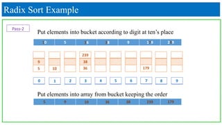
10 5 36 38 9 179 239

Radix Sort Example
Put elements into bucket according to digit at ten’s place
Pass-2
210 3 4 5 6 7 8 9
9
179
239
38
105 36
10 5 36 38 9 179 239
5 9 10 36 38 239 179

Radix Sort Example
Put elements into bucket according to digit at hundred’s place
Pass-3
210 3 4 5 6 7 8 9
9
239179
38
5
36
5 9 10 36 38 239 179
5 9 10 36 38 179 239
10

• Assumption: input is in the range 1..k
• Basic idea:
• Count number of elements k  each element i
• Use that number to place i in position k of sorted array
• No comparisons! Runs in time O(n + k)
• Stable sort
• Does not sort in place:
• O(n) array to hold sorted output
• O(k) array for scratch storage
Counting Sort

Counting Sort Algorithm
for i  1 to k
do C[i]  0
1.
for j  1 to n
do C[A[ j]]  C[A[ j]] + 1
2.
for i  2 to k
do C[i]  C[i] + C[i–1]
3.
for j  n downto 1
do B[C[A[ j]]]  A[ j]
C[A[ j]]  C[A[ j]] – 1
4.
Initialize
Count
Compute running sum
Re-arrange

•Input : A[1 . . n], where A[ j] {1, 2, …, k} .
•Output : B[1 . . n], sorted.
•Auxiliary storage : C[1 . . k] .
Counting Sort Example
A: 4 1 3 4 3
B:
1 2 3 4 5
C:
1 2 3 4

Loop 1: initialization
for i  1 to k
do C[i]  0
1.
A:
1 2 3 4 5
C: 0 0 0
1 2 3 4
4 1 3 4 3 0
B:

C: 0
1 2 3 4
A:
1 2 3 4 5
4 1 3 4 3 1 0 0 01 12 2
Loop 2: count
for j  1 to n
do C[A[ j]]  C[A[ j]] + 1
2.
B:

C:
1 2 3 4
A:
1 2 3 4 5
4 1 3 4 3 1 0 2 2
B:
1 0 2 2
1 2 3 4
1 01 23 25
Loop 3: compute running sum
for i  2 to k
do C[i]  C[i] + C[i–1]
3.

C:
1 2 3 4
A:
1 2 3 4 5
4 1 3 4 3
B:
1 0 2 2
1 2 3 4
1
Loop 4: re-arrange
3
3 1 332 5
do B[C[A[ j]]]  A[ j]
C[A[ j]]  C[A[ j]] – 1
4.

C:
1 2 3 4
A:
1 2 3 4 5
4 1 3 4
B:
1 0 2 2
Loop 4: re-arrange
1 2 3 4
1 1 2 5
4 3
543
do B[C[A[ j]]]  A[ j]
C[A[ j]]  C[A[ j]] – 1
4.
4

C:
1 2 3 4
A:
1 2 3 4 5
4 1 3
B:
1 0 2 2
Loop 4: re-arrange
1 2 3 4
1 1 2
3
3
4 3
3 4 21 4
do B[C[A[ j]]]  A[ j]
C[A[ j]]  C[A[ j]] – 1
4.

C:
1 2 3 4
A:
1 2 3 4 5
4 1
B:
1 0 2 2
Loop 4: re-arrange
1 2 3 4
1
1
1 13 3 4
3 4 3
0 1 1 4
do B[C[A[ j]]]  A[ j]
C[A[ j]]  C[A[ j]] – 1
4.

C:
1 2 3 4
A:
1 2 3 4 5
4
B:
1 0 2 2
Loop 4: re-arrange
1 2 3 4
0 1 1 41 3 3
4
4
1 3 4 3
4 43
do B[C[A[ j]]]  A[ j]
C[A[ j]]  C[A[ j]] – 1
4.

1 3 3 4 4
Sorted elements:
• The initialization of the Count array, and the second for loop which performs a
prefix sum on the count array, each iterate at most k + 1 times and therefore
take O(k) time.
• The other two for loops, and the initialization of the output array, each
take O(n) time. Therefore the time for the whole algorithm is the sum of the
times for these steps, O(n + k).

Analysis and Design of Algorithms -Sorting Algorithms and analysis

Analysis and Design of Algorithms -Sorting Algorithms and analysis

Recommended

More Related Content

What's hot (20)

Similar to Analysis and Design of Algorithms -Sorting Algorithms and analysis (20)

More from Radhika Talaviya (16)

Recently uploaded (20)

Analysis and Design of Algorithms -Sorting Algorithms and analysis