


![Initialization of Array
1. The simplest way to initialize an array is by using the index of each
element.
marks[0]=80;//initialization of array
marks[1]=60;
marks[2]=70;
marks[3]=85;
marks[4]=75;
2. To insert values to it, use a comma-separated list, inside curly
braces:
int myNumbers[] = {25, 50, 75, 100, 70};](https://image.slidesharecdn.com/unit1-240303101304-6d298e08/85/Basic-of-array-and-data-structure-data-structure-basics-array-address-calculation-sparse-matrix-9-320.jpg)
![Array initialization (Alternative)
• To insert values to it, use a comma-separated list,
inside curly braces:
int myNumbers[] = {25, 50, 75, 100};](https://image.slidesharecdn.com/unit1-240303101304-6d298e08/85/Basic-of-array-and-data-structure-data-structure-basics-array-address-calculation-sparse-matrix-10-320.jpg)
![Calculating the address of any element In the 1-D
array:
To find the address of an element in an array the following formula is
used-
Address of A[I] = B + W * (I – LB)
I = Subset of element whose address to be found,
B = Base address,
W = Storage size of one element store in any array(in byte),
LB = Lower Limit/Lower Bound of subscript(If not specified assume
zero).](https://image.slidesharecdn.com/unit1-240303101304-6d298e08/85/Basic-of-array-and-data-structure-data-structure-basics-array-address-calculation-sparse-matrix-11-320.jpg)
![Two Dimensional Array
• The two-dimensional array can be defined as an array of 1- D arrays.
The 2D array is organized as matrices which can be represented as the
collection of rows and columns.
• In C, 2-Dimensional arrays can be declared as follows:
Syntax:
Datatype arrayname[size1/row][size2/column];
• Example:
The meaning of the above representation can be understood as:
• The memory allocated to variable b is of data type int.
• The data is being represented in the form of 2 rows and 3 columns.](https://image.slidesharecdn.com/unit1-240303101304-6d298e08/85/Basic-of-array-and-data-structure-data-structure-basics-array-address-calculation-sparse-matrix-12-320.jpg)


![Calculating the address of any element In the 2-D array:
• To find the address of any element in a 2-Dimensional array there are the following two
ways-
• Row Major Order
• Column Major Order
a) Row Major Order
To find the address of the element using row-major order uses the following formula in
A[M][N]:
Address of A[I][J] = B + W * ((I – LR) * N + (J – LC))
I = Row Subset of an element whose address to be found,
J = Column Subset of an element whose address to be found,
B = Base address, W = Storage size of one element store in an array(in byte),
LR = Lower Limit of row/start row index of the matrix(If not given assume it as zero),
LC = Lower Limit of column/start column index of the matrix(If not given assume it zero)
N = Number of column given in the matrix.](https://image.slidesharecdn.com/unit1-240303101304-6d298e08/85/Basic-of-array-and-data-structure-data-structure-basics-array-address-calculation-sparse-matrix-15-320.jpg)
![a) Column Major Order
To find the address of the element using row-major order uses the following formula in
A[M][N]:
Address of A[I][J] = B + W * ((J – LC) * M + (I – LR))
I = Row Subset of an element whose address to be found,
J = Column Subset of an element whose address to be found,
B = Base address,
W = Storage size of one element store in any array(in byte),
LR = Lower Limit of row/start row index of matrix(If not given assume it as zero),
LC = Lower Limit of column/start column index of matrix(If not given assume it zero),
M = Number of rows given in the matrix.](https://image.slidesharecdn.com/unit1-240303101304-6d298e08/85/Basic-of-array-and-data-structure-data-structure-basics-array-address-calculation-sparse-matrix-16-320.jpg)
![• Example: Given an array arr[1………10][1………15] with a base value of
100 and the size of each element is 1 Byte in memory find the
address of arr[8][6] with the help of column-major order.
• Formula: used
Address of A[I][J] = B + W * ((J – LC) * M + (I – LR))
Address of A[8][6] = 100 + 1 * ((6 – 1) * 10 + (8 – 1))
= 100 + 1 * ((5) * 10 + (7))
= 100 + 1 * (57)
Address of A[I][J] = 157](https://image.slidesharecdn.com/unit1-240303101304-6d298e08/85/Basic-of-array-and-data-structure-data-structure-basics-array-address-calculation-sparse-matrix-17-320.jpg)
![Example: A double dimensional array Arr[-10…12, -15…20] contains
elements in such a way that each element occupies 4 byte memory
space. If the base address array is 2000. Find the address of the array
element Arr[-6][8]. Perform the calculations in Row-Major form and
Column-Major form.
Ans: Solution:
• B= 2000
• I= -6
• J= 8
• R0= -10
• C0= -15
• Number of rows (M) = [12-(-10)]+1=23
• Number of columns (N) = [20-(-15)]+1=36
• W=4](https://image.slidesharecdn.com/unit1-240303101304-6d298e08/85/Basic-of-array-and-data-structure-data-structure-basics-array-address-calculation-sparse-matrix-18-320.jpg)
![Row wise Calculation:
Address of array element
Arr[-6][8]= B+ W [N (I – R0) + (J – C0)]
= 2000+4[36(-6-(-10))+(8-(-15))]
= 2000+4[36(-6+10)+(8+15)]
= 2000+4*[(36*4)+23]
= 2000+4*[144+23]
= 2000+4*167
= 2000+668
= 2668
Column wise Calculation:
Address of array element
Arr[-6][8]= B+ W [(I – R0) + M (J – C0)]
= 2000+4[(-6-(-10))+23(8-(-15))]
= 2000+4[(-6+10)+23(8+15)]
= 2000+4*[4+(23*23)]
= 2000+4*[4+529]
= 2000+4*533
= 2000+2132
= 4132](https://image.slidesharecdn.com/unit1-240303101304-6d298e08/85/Basic-of-array-and-data-structure-data-structure-basics-array-address-calculation-sparse-matrix-19-320.jpg)
![• An array X [-15……….10, 15……………40] requires one byte of storage. If
beginning location is 1500 determine the location of X [15][20] in row
major and column major order.
• Row Major: 2285
• Column Major: 1660](https://image.slidesharecdn.com/unit1-240303101304-6d298e08/85/Basic-of-array-and-data-structure-data-structure-basics-array-address-calculation-sparse-matrix-20-320.jpg)


![int main()
{ int sparseMatrix[4][5] =
{
{0 , 0 , 5 , 1 , 0 },
{0 , 0 , 0 , 7 , 0 },
{1 , 0 , 0 , 0 , 9 },
{0 , 2 , 0 , 0 , 0 }
};
int size = 0;
for (int i = 0; i < 4; i++)
for (int j = 0; j < 5; j++)
if (sparseMatrix[i][j] != 0)
size++;
int compactMatrix[size][3];
int k = 0;
for (int i = 0; i < 4; i++)
for (int j = 0; j < 5; j++)
if (sparseMatrix[i][j] != 0)
{
compactMatrix[k][0] = i;
compactMatrix[k][1] = j;
compactMatrix[k][2] = sparseMatrix[i][j];
k++;}
cout<<" R C Vn";
for (int j=0; j<size; j++)
{
for (int i=0; i<3; i++)
cout <<" "<< compactMatrix[j][i];
cout <<"n";
}
return 0;
}](https://image.slidesharecdn.com/unit1-240303101304-6d298e08/85/Basic-of-array-and-data-structure-data-structure-basics-array-address-calculation-sparse-matrix-26-320.jpg)


![Linear Search ( Array A, Value x)
Step 1: Set i to 1
Step 2: if i > n then go to step 7
Step 3: if A[i] = x then go to step 6
Step 4: Set i to i + 1
Step 5: Go to Step 2
Step 6: Print Element x Found at index i and go to step 8
Step 7: Print element not found
Step 8: Exit](https://image.slidesharecdn.com/unit1-240303101304-6d298e08/85/Basic-of-array-and-data-structure-data-structure-basics-array-address-calculation-sparse-matrix-29-320.jpg)
![int main(void)
{ int i, x, flag=0, arr[] = { 2, 3, 4, 10, 40, 34, 21, 78, 50 };
int N = sizeof(arr) / sizeof(arr[0]);
cout<<"Enter the value of element: ";
cin >> x;
for (i = 0; i < N; i++)
{ if (arr[i] == x)
{
flag=1;
break;
}
else
flag == 0;
}
if(flag == 1)
cout<<"Element is present at place: " << i+1;
else
cout << "Element is not present in array. ";
}](https://image.slidesharecdn.com/unit1-240303101304-6d298e08/85/Basic-of-array-and-data-structure-data-structure-basics-array-address-calculation-sparse-matrix-30-320.jpg)
![#include <iostream>
using namespace std;
int binarySearch(int arr[], int num, int beg, int end)
{
int mid = beg + (end - 1) / 2;
if (arr[mid] == num)
return mid;
else if (num > arr[mid])
binarySearch (arr, num, mid+1, end);
else if (num < arr[mid])
binarySearch (arr, num, beg , mid-1);
}
int main(void)
{
int x , arr[] = { 2, 3, 4, 10, 40, 50, 55, 60, 70 };
cout<<"Enter the value of element: ";
cin >> x;
int n = sizeof(arr) / sizeof(arr[0]);
int result = binarySearch(arr, x, 0 , n-1);
cout << "Element is present at: " << result+1;
return 0;
}
Binary search](https://image.slidesharecdn.com/unit1-240303101304-6d298e08/85/Basic-of-array-and-data-structure-data-structure-basics-array-address-calculation-sparse-matrix-31-320.jpg)

![Algorithm
begin BubbleSort(arr)
for all array elements
if arr[i] > arr[i+1]
swap(arr[i], arr[i+1])
end if
end for
return arr
end BubbleSort](https://image.slidesharecdn.com/unit1-240303101304-6d298e08/85/Basic-of-array-and-data-structure-data-structure-basics-array-address-calculation-sparse-matrix-34-320.jpg)
![#include<stdio.h>
void main ()
{
int i, j,temp;
int a[] = { 10, 9, 7, 101, 23, 44, 12, 78, 34, 23};
int n=sizeof(a)/sizeof(a[0]);
for(i = 0; i<n; i++)
{
for(j = 0; j<n-i-1; j++)
{
if(a[j] > a[j+1])
{
temp = a[j];
a[j] = a[j+1];
a[j+1] = temp;
}
}
}
printf("Printing Sorted Element List ...n");
for(i = 0; i<n; i++)
{
printf("%dn",a[i]);
}
}
Sorting an array using bubble sort](https://image.slidesharecdn.com/unit1-240303101304-6d298e08/85/Basic-of-array-and-data-structure-data-structure-basics-array-address-calculation-sparse-matrix-35-320.jpg)


![int main() {
int i, data[] = {39, 20, 12, 10, 54, 15, 2};
int size = sizeof(data) / sizeof(data[0]);
selectionSort(data, size);
printf("Sorted array in Acsending Order:n");
for (i = 0; i < size; i++)
printf("%d ", data[i]);
}
#include <stdio.h>
void swap(int *a, int *b) {
int temp = *a;
*a = *b;
*b = temp;
}
void selectionSort(int array[], int size)
{ int step, i;
for (step = 0; step < size - 1; step++)
{ int min_idx = step;
for ( i = step + 1; i < size; i++)
{
if (array[i] < array[min_idx])
min_idx = i;
}
swap(&array[min_idx], &array[step]);
}
}](https://image.slidesharecdn.com/unit1-240303101304-6d298e08/85/Basic-of-array-and-data-structure-data-structure-basics-array-address-calculation-sparse-matrix-38-320.jpg)


![#include <stdio.h>
void insertionSort(int arr[], int n)
{
int i, key, j;
for (i = 1; i < n; i++) {
key = arr[i];
j = i - 1;
while (j >= 0 && arr[j] > key)
{
arr[j + 1] = arr[j];
j = j - 1;
}
arr[j + 1] = key;
}
}
int main()
{
int i, arr[] = { 102, 98, 13, 51, 75, 66 };
int n = sizeof(arr) / sizeof(arr[0]);
insertionSort(arr, n);
printf("Sorted array is: n");
for (i = 0; i < n; i++)
printf("%d ", arr[i]);
return 0;
}](https://image.slidesharecdn.com/unit1-240303101304-6d298e08/85/Basic-of-array-and-data-structure-data-structure-basics-array-address-calculation-sparse-matrix-41-320.jpg)

![Radix Sort
• Radix Sort is a Sorting algorithm that is useful when there is a constant 'd'
such that all keys are d digit numbers.
• To execute Radix Sort, for p =1 towards 'd' sort the numbers with respect to
the pth digits from the right using any linear time stable sort.
• The following procedure assumes that each element in the n-element array
A has d digits, where digit 1 is the lowest order digit and digit d is the
highest-order digit.
• Radix sort uses counting sort as a subroutine to sort.
• Following algorithm that sorts A [1.n] where each number is d digits long.
• RADIX-SORT (array A, int n, int d)
1. for i ← 1 to d
2. do stably sort A to sort array A on digit i](https://image.slidesharecdn.com/unit1-240303101304-6d298e08/85/Basic-of-array-and-data-structure-data-structure-basics-array-address-calculation-sparse-matrix-43-320.jpg)


![#include <stdlib.h>
void merge(int arr[], int l, int m, int r)
{
int i, j, k;
int n1 = m - l + 1;
int n2 = r - m;
/* create temp arrays */
int L[n1], R[n2];
/* Copy data to temp arrays L[] and R[] */
for (i = 0; i < n1; i++)
L[i] = arr[l + i];
for (j = 0; j < n2; j++)
R[j] = arr[m + 1 + j];
/* Merge the temp arrays back into arr[l..r]*/
i = 0; // Initial index of first subarray
j = 0; // Initial index of second subarray
k = l; // Initial index of merged subarray
while (i < n1 && j < n2) {
if (L[i] <= R[j]) {
arr[k] = L[i];
i++;
}
else {
arr[k] = R[j];
j++;
}
k++;
}
/* Copy the remaining elements of L[], if there
are any */
while (i < n1) {
arr[k] = L[i];
i++;
k++;
}
/* Copy the remaining elements of R[], if there
are any */
while (j < n2) {
arr[k] = R[j];
j++;
k++;
}
}](https://image.slidesharecdn.com/unit1-240303101304-6d298e08/85/Basic-of-array-and-data-structure-data-structure-basics-array-address-calculation-sparse-matrix-48-320.jpg)
![void mergeSort(int arr[], int l, int r)
{
if (l < r) {
// Same as (l+r)/2, but avoids overflow for
// large l and h
int m = l + (r - l) / 2;
// Sort first and second halves
mergeSort(arr, l, m);
mergeSort(arr, m + 1, r);
merge(arr, l, m, r);
}
}
void printArray(int A[], int size)
{
int i;
for (i = 0; i < size; i++)
printf("%d ", A[i]);
printf("n");
}
int main()
{
int arr[] = { 10, 13, 5, 76, 17, 33, 22, 54, 9, 43, 27 };
int arr_size = sizeof(arr) / sizeof(arr[0]);
printf("Given array is n");
printArray(arr, arr_size);
mergeSort(arr, 0, arr_size - 1);
printf("nSorted array is n");
printArray(arr, arr_size);
return 0;
}](https://image.slidesharecdn.com/unit1-240303101304-6d298e08/85/Basic-of-array-and-data-structure-data-structure-basics-array-address-calculation-sparse-matrix-49-320.jpg)

![#include <iostream>
using namespace std;
void shellSort(int arr[], int n)
{
for (int gap = n/2; gap > 0; gap /= 2)
{
for (int i = gap; i < n; i++)
{
int temp = arr[i];
for (int j = i; j >= gap && arr[j - gap] > temp; j -= gap)
arr[j] = arr[j - gap];
arr[j] = temp;
}
}
}
void printArray(int arr[], int n)
{
for (int i=0; i<n; i++)
cout << arr[i] << " ";
}
int main()
{
int arr[] = {12, 34, 54, 2, 3, 23, 1, 56, 39}, i;
int n = sizeof(arr)/sizeof(arr[0]);
cout << "Array before sorting: n";
printArray(arr, n);
shellSort(arr, n);
cout << "nArray after sorting: n";
printArray(arr, n);
return 0;
}](https://image.slidesharecdn.com/unit1-240303101304-6d298e08/85/Basic-of-array-and-data-structure-data-structure-basics-array-address-calculation-sparse-matrix-51-320.jpg)

Basic of array and data structure, data structure basics, array, address calculation, sparse matrix
- 1. Unit 1
- 2. Content
- 3. Data Structure • Data structure is a storage that is used to store and organize data. • It is a way of arranging data on a computer so that it can be accessed and updated efficiently. • It is also used for processing, retrieving, and storing data. There are different basic and advanced types of data structures that are used in almost every program or software system that has been developed. So we must have good knowledge about data structures.
- 5. • Linear data structure: Data structure in which data elements are arranged sequentially or linearly, where each element is attached to its previous and next adjacent elements, is called a linear data structure. Examples of linear data structures are array, stack, queue, linked list, etc. • Static data structure: Static data structure has a fixed memory size. It is easier to access the elements in a static data structure. An example of this data structure is an array. • Dynamic data structure: In dynamic data structure, the size is not fixed. It can be randomly updated during the runtime which may be considered efficient concerning the memory (space) complexity of the code. Examples of this data structure are queue, stack, etc. • Non-linear data structure: Data structures where data elements are not placed sequentially or linearly are called non-linear data structures. In a non-linear data structure, we can’t traverse all the elements in a single run only. Examples of non-linear data structures are trees and graphs.
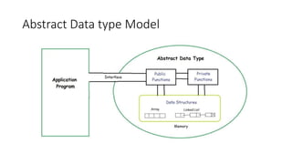
- 6. Abstract Data type • Abstract Data type (ADT) is a type (or class) for objects whose behavior is defined by a set of values and a set of operations. • The definition of ADT only mentions what operations are to be performed but not how these operations will be implemented. It does not specify how data will be organized in memory and what algorithms will be used for implementing the operations. It is called “abstract” because it gives an implementation-independent view.
- 7. Abstract Data type Model
- 8. Array • An array is defined as the collection of similar type of data items stored at contiguous memory locations. • Arrays are the derived data type in programming language which can store the primitive type of data such as int, char, double, float, etc. • The array is the simplest data structure where each data element can be randomly accessed by using its index number.
- 9. Initialization of Array 1. The simplest way to initialize an array is by using the index of each element. marks[0]=80;//initialization of array marks[1]=60; marks[2]=70; marks[3]=85; marks[4]=75; 2. To insert values to it, use a comma-separated list, inside curly braces: int myNumbers[] = {25, 50, 75, 100, 70};
- 10. Array initialization (Alternative) • To insert values to it, use a comma-separated list, inside curly braces: int myNumbers[] = {25, 50, 75, 100};
- 11. Calculating the address of any element In the 1-D array: To find the address of an element in an array the following formula is used- Address of A[I] = B + W * (I – LB) I = Subset of element whose address to be found, B = Base address, W = Storage size of one element store in any array(in byte), LB = Lower Limit/Lower Bound of subscript(If not specified assume zero).
- 12. Two Dimensional Array • The two-dimensional array can be defined as an array of 1- D arrays. The 2D array is organized as matrices which can be represented as the collection of rows and columns. • In C, 2-Dimensional arrays can be declared as follows: Syntax: Datatype arrayname[size1/row][size2/column]; • Example: The meaning of the above representation can be understood as: • The memory allocated to variable b is of data type int. • The data is being represented in the form of 2 rows and 3 columns.
- 15. Calculating the address of any element In the 2-D array: • To find the address of any element in a 2-Dimensional array there are the following two ways- • Row Major Order • Column Major Order a) Row Major Order To find the address of the element using row-major order uses the following formula in A[M][N]: Address of A[I][J] = B + W * ((I – LR) * N + (J – LC)) I = Row Subset of an element whose address to be found, J = Column Subset of an element whose address to be found, B = Base address, W = Storage size of one element store in an array(in byte), LR = Lower Limit of row/start row index of the matrix(If not given assume it as zero), LC = Lower Limit of column/start column index of the matrix(If not given assume it zero) N = Number of column given in the matrix.
- 16. a) Column Major Order To find the address of the element using row-major order uses the following formula in A[M][N]: Address of A[I][J] = B + W * ((J – LC) * M + (I – LR)) I = Row Subset of an element whose address to be found, J = Column Subset of an element whose address to be found, B = Base address, W = Storage size of one element store in any array(in byte), LR = Lower Limit of row/start row index of matrix(If not given assume it as zero), LC = Lower Limit of column/start column index of matrix(If not given assume it zero), M = Number of rows given in the matrix.
- 17. • Example: Given an array arr[1………10][1………15] with a base value of 100 and the size of each element is 1 Byte in memory find the address of arr[8][6] with the help of column-major order. • Formula: used Address of A[I][J] = B + W * ((J – LC) * M + (I – LR)) Address of A[8][6] = 100 + 1 * ((6 – 1) * 10 + (8 – 1)) = 100 + 1 * ((5) * 10 + (7)) = 100 + 1 * (57) Address of A[I][J] = 157
- 18. Example: A double dimensional array Arr[-10…12, -15…20] contains elements in such a way that each element occupies 4 byte memory space. If the base address array is 2000. Find the address of the array element Arr[-6][8]. Perform the calculations in Row-Major form and Column-Major form. Ans: Solution: • B= 2000 • I= -6 • J= 8 • R0= -10 • C0= -15 • Number of rows (M) = [12-(-10)]+1=23 • Number of columns (N) = [20-(-15)]+1=36 • W=4
- 19. Row wise Calculation: Address of array element Arr[-6][8]= B+ W [N (I – R0) + (J – C0)] = 2000+4[36(-6-(-10))+(8-(-15))] = 2000+4[36(-6+10)+(8+15)] = 2000+4*[(36*4)+23] = 2000+4*[144+23] = 2000+4*167 = 2000+668 = 2668 Column wise Calculation: Address of array element Arr[-6][8]= B+ W [(I – R0) + M (J – C0)] = 2000+4[(-6-(-10))+23(8-(-15))] = 2000+4[(-6+10)+23(8+15)] = 2000+4*[4+(23*23)] = 2000+4*[4+529] = 2000+4*533 = 2000+2132 = 4132
- 20. • An array X [-15……….10, 15……………40] requires one byte of storage. If beginning location is 1500 determine the location of X [15][20] in row major and column major order. • Row Major: 2285 • Column Major: 1660
- 21. • Sparse matrices are those matrices that have the majority of their elements equal to zero. • In other words, the sparse matrix can be defined as the matrix that has a greater number of zero elements than the non-zero elements. Sparse Matrix
- 23. • Linked List representation of the sparse matrix a node in the linked list representation consists of four fields. The four fields of the linked list are given as follows - • Row - It represents the index of the row where the non-zero element is located. • Column - It represents the index of the column where the non-zero element is located. • Value - It is the value of the non-zero element that is located at the index (row, column). • Next node - It stores the address of the next node.
- 25. Types of sparse matrix •Regular sparse matrices •Irregular sparse matrices / Non - regular sparse matrices
- 26. int main() { int sparseMatrix[4][5] = { {0 , 0 , 5 , 1 , 0 }, {0 , 0 , 0 , 7 , 0 }, {1 , 0 , 0 , 0 , 9 }, {0 , 2 , 0 , 0 , 0 } }; int size = 0; for (int i = 0; i < 4; i++) for (int j = 0; j < 5; j++) if (sparseMatrix[i][j] != 0) size++; int compactMatrix[size][3]; int k = 0; for (int i = 0; i < 4; i++) for (int j = 0; j < 5; j++) if (sparseMatrix[i][j] != 0) { compactMatrix[k][0] = i; compactMatrix[k][1] = j; compactMatrix[k][2] = sparseMatrix[i][j]; k++;} cout<<" R C Vn"; for (int j=0; j<size; j++) { for (int i=0; i<3; i++) cout <<" "<< compactMatrix[j][i]; cout <<"n"; } return 0; }
- 27. Searching • Linear Search • Binary Search
- 29. Linear Search ( Array A, Value x) Step 1: Set i to 1 Step 2: if i > n then go to step 7 Step 3: if A[i] = x then go to step 6 Step 4: Set i to i + 1 Step 5: Go to Step 2 Step 6: Print Element x Found at index i and go to step 8 Step 7: Print element not found Step 8: Exit
- 30. int main(void) { int i, x, flag=0, arr[] = { 2, 3, 4, 10, 40, 34, 21, 78, 50 }; int N = sizeof(arr) / sizeof(arr[0]); cout<<"Enter the value of element: "; cin >> x; for (i = 0; i < N; i++) { if (arr[i] == x) { flag=1; break; } else flag == 0; } if(flag == 1) cout<<"Element is present at place: " << i+1; else cout << "Element is not present in array. "; }
- 31. #include <iostream> using namespace std; int binarySearch(int arr[], int num, int beg, int end) { int mid = beg + (end - 1) / 2; if (arr[mid] == num) return mid; else if (num > arr[mid]) binarySearch (arr, num, mid+1, end); else if (num < arr[mid]) binarySearch (arr, num, beg , mid-1); } int main(void) { int x , arr[] = { 2, 3, 4, 10, 40, 50, 55, 60, 70 }; cout<<"Enter the value of element: "; cin >> x; int n = sizeof(arr) / sizeof(arr[0]); int result = binarySearch(arr, x, 0 , n-1); cout << "Element is present at: " << result+1; return 0; } Binary search
- 32. Sorting • Sorting is a operation to arrange the elements of an array in ascending or descending order. Types of sorting: • Bubble sort • Insertion sort • Selection sort
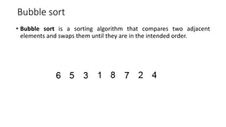
- 33. Bubble sort • Bubble sort is a sorting algorithm that compares two adjacent elements and swaps them until they are in the intended order.
- 34. Algorithm begin BubbleSort(arr) for all array elements if arr[i] > arr[i+1] swap(arr[i], arr[i+1]) end if end for return arr end BubbleSort
- 35. #include<stdio.h> void main () { int i, j,temp; int a[] = { 10, 9, 7, 101, 23, 44, 12, 78, 34, 23}; int n=sizeof(a)/sizeof(a[0]); for(i = 0; i<n; i++) { for(j = 0; j<n-i-1; j++) { if(a[j] > a[j+1]) { temp = a[j]; a[j] = a[j+1]; a[j+1] = temp; } } } printf("Printing Sorted Element List ...n"); for(i = 0; i<n; i++) { printf("%dn",a[i]); } } Sorting an array using bubble sort
- 36. Selection Sort
- 37. Algorithm Follow the below steps to solve the problem: • Initialize minimum value(min_idx) to location 0. • Traverse the array to find the minimum element in the array. • While traversing if any element smaller than min_idx is found then swap both the values. • Then, increment min_idx to point to the next element. • Repeat until the array is sorted.
- 38. int main() { int i, data[] = {39, 20, 12, 10, 54, 15, 2}; int size = sizeof(data) / sizeof(data[0]); selectionSort(data, size); printf("Sorted array in Acsending Order:n"); for (i = 0; i < size; i++) printf("%d ", data[i]); } #include <stdio.h> void swap(int *a, int *b) { int temp = *a; *a = *b; *b = temp; } void selectionSort(int array[], int size) { int step, i; for (step = 0; step < size - 1; step++) { int min_idx = step; for ( i = step + 1; i < size; i++) { if (array[i] < array[min_idx]) min_idx = i; } swap(&array[min_idx], &array[step]); } }
- 39. Insertion Sort
- 40. Insertion Sort Algorithm The simple steps of achieving the insertion sort are listed as follows - • Step 1 - If the element is the first element, assume that it is already sorted. Return 1. • Step2 - Pick the next element, and store it separately in a key. • Step3 - Now, compare the key with all elements in the sorted array. • Step 4 - If the element in the sorted array is smaller than the current element, then move to the next element. Else, shift greater elements in the array towards the right. • Step 5 - Insert the value. • Step 6 - Repeat until the array is sorted.
- 41. #include <stdio.h> void insertionSort(int arr[], int n) { int i, key, j; for (i = 1; i < n; i++) { key = arr[i]; j = i - 1; while (j >= 0 && arr[j] > key) { arr[j + 1] = arr[j]; j = j - 1; } arr[j + 1] = key; } } int main() { int i, arr[] = { 102, 98, 13, 51, 75, 66 }; int n = sizeof(arr) / sizeof(arr[0]); insertionSort(arr, n); printf("Sorted array is: n"); for (i = 0; i < n; i++) printf("%d ", arr[i]); return 0; }
- 42. Time and space complexity
- 43. Radix Sort • Radix Sort is a Sorting algorithm that is useful when there is a constant 'd' such that all keys are d digit numbers. • To execute Radix Sort, for p =1 towards 'd' sort the numbers with respect to the pth digits from the right using any linear time stable sort. • The following procedure assumes that each element in the n-element array A has d digits, where digit 1 is the lowest order digit and digit d is the highest-order digit. • Radix sort uses counting sort as a subroutine to sort. • Following algorithm that sorts A [1.n] where each number is d digits long. • RADIX-SORT (array A, int n, int d) 1. for i ← 1 to d 2. do stably sort A to sort array A on digit i
- 44. Overall time complexity is θ(dn) = θ(n) where d is constant Overall space complexity is θ(n).
- 45. Merge Sort Merge sort is defined as a sorting algorithm that works by dividing an array into smaller subarrays, sorting each subarray, and then merging the sorted subarrays back together to form the final sorted array.
- 47. Algorithm step 1: start step 2: declare array and left, right, mid variable step 3: perform merge function. if left > right return mid= (left+right)/2 mergesort(array, left, mid) mergesort(array, mid+1, right) merge(array, left, mid, right) step 4: Stop
- 48. #include <stdlib.h> void merge(int arr[], int l, int m, int r) { int i, j, k; int n1 = m - l + 1; int n2 = r - m; /* create temp arrays */ int L[n1], R[n2]; /* Copy data to temp arrays L[] and R[] */ for (i = 0; i < n1; i++) L[i] = arr[l + i]; for (j = 0; j < n2; j++) R[j] = arr[m + 1 + j]; /* Merge the temp arrays back into arr[l..r]*/ i = 0; // Initial index of first subarray j = 0; // Initial index of second subarray k = l; // Initial index of merged subarray while (i < n1 && j < n2) { if (L[i] <= R[j]) { arr[k] = L[i]; i++; } else { arr[k] = R[j]; j++; } k++; } /* Copy the remaining elements of L[], if there are any */ while (i < n1) { arr[k] = L[i]; i++; k++; } /* Copy the remaining elements of R[], if there are any */ while (j < n2) { arr[k] = R[j]; j++; k++; } }
- 49. void mergeSort(int arr[], int l, int r) { if (l < r) { // Same as (l+r)/2, but avoids overflow for // large l and h int m = l + (r - l) / 2; // Sort first and second halves mergeSort(arr, l, m); mergeSort(arr, m + 1, r); merge(arr, l, m, r); } } void printArray(int A[], int size) { int i; for (i = 0; i < size; i++) printf("%d ", A[i]); printf("n"); } int main() { int arr[] = { 10, 13, 5, 76, 17, 33, 22, 54, 9, 43, 27 }; int arr_size = sizeof(arr) / sizeof(arr[0]); printf("Given array is n"); printArray(arr, arr_size); mergeSort(arr, 0, arr_size - 1); printf("nSorted array is n"); printArray(arr, arr_size); return 0; }
- 50. Shell sort • Shell sort is mainly a variation of Insertion Sort. • In insertion sort, we move elements only one position ahead. When an element has to be moved far ahead, many movements are involved. • The idea of ShellSort is to allow the exchange of far items. • In Shell sort, we make the array h-sorted for a large value of h. • We keep reducing the value of h until it becomes 1. • An array is said to be h-sorted if all sublists of every h’th element are sorted.
- 51. #include <iostream> using namespace std; void shellSort(int arr[], int n) { for (int gap = n/2; gap > 0; gap /= 2) { for (int i = gap; i < n; i++) { int temp = arr[i]; for (int j = i; j >= gap && arr[j - gap] > temp; j -= gap) arr[j] = arr[j - gap]; arr[j] = temp; } } } void printArray(int arr[], int n) { for (int i=0; i<n; i++) cout << arr[i] << " "; } int main() { int arr[] = {12, 34, 54, 2, 3, 23, 1, 56, 39}, i; int n = sizeof(arr)/sizeof(arr[0]); cout << "Array before sorting: n"; printArray(arr, n); shellSort(arr, n); cout << "nArray after sorting: n"; printArray(arr, n); return 0; }
- 52. Complexity Of all sorting algorithm