Classification: MNIST, training a Binary classifier, performance measure, multiclass classification, error analysis, multi label classification, multi output classification.

Introduction to Classification with
MNIST
Understanding the Basics of Image Classification in
Machine Learning
By.
Dr. Ravi Kumar B N
Assistant Professor, Dept. of ISE
Module2 PartI

Definition of Classification
Classification is a supervised machine learning task where the goal is to assign input
data to predefined categories or classes. A model learns from labeled training data and
then predicts the class labels for new, unseen data.
Types of Classification
1. Binary Classification
•Involves only two classes (e.g., Yes/No, Spam/Not Spam, Fraud/Not Fraud).
•Example: Email spam detection (spam or not spam).
2. Multi-Class Classification
•Involves more than two classes, where each instance belongs to exactly one class.
•Example: Handwritten digit recognition (0-9).
3. Multi-Label Classification
•Each instance can belong to multiple classes simultaneously.
•Example: A movie can be categorized as both "Action" and "Sci-Fi".
4. Multi-Output Classification (also called multi-target classification)
• model predicts multiple labels (outputs) for each input sample. Unlike multi-label classification
(where each instance belongs to multiple categories), here, each output can be treated as a
separate classification problem.
• image and predicts both the digit (0-9) and its color (red, blue, etc.).

Classification Algorithms
1.Logistic Regression – A linear model that estimates probabilities using the sigmoid function.
Example: Predicting if a customer will buy a product (Yes/No).
2.K-Nearest Neighbors (KNN) – Classifies a data point based on the majority class of its k-nearest
neighbors.
Example: Handwriting recognition.
3.Support Vector Machine (SVM) – Finds the optimal hyperplane that maximizes the margin between
classes.
Example: Face detection in images.
4.Decision Tree – A tree-like model that splits data based on feature conditions.
Example: Loan approval prediction.
5.Random Forest – An ensemble of decision trees that improves accuracy and reduces overfitting.
Example: Medical diagnosis classification.
6.Naïve Bayes – A probabilistic model based on Bayes' theorem with the assumption of feature
independence.
Example: Spam email filtering.
7.Artificial Neural Networks (ANNs) – Deep learning models inspired by the human brain for complex
patterns.
Example: Image classification (e.g., cats vs. dogs).

MNIST Dataset Overview
The MNIST (Modified National Institute of Standards and Technology)
dataset contains handwritten digits is a famous benchmark in machine
learning and computer vision. It consists of:
•70,000 grayscale images (28x28 pixels each).
•10 classes (digits 0-9).
•60,000 training images and 10,000 test images.
•Handwritten digit recognition is a common task using MNIST.
This set is often called the “hello world” of Machine Learning whenever people come up
with a new classification algorithm they are curious to see how it will perform on MNIST

What is Scikit-Learn?
"Scientific Toolkit for Machine Learning"
Scikit-Learn is a popular Python machine learning library built on NumPy, SciPy,
and Matplotlib. It provides simple and efficient tools for data mining, analysis, and
machine learning tasks.
Scikit-Learn follows a simple "fit → predict → evaluate" workflow.

The following code fetches the MNIST dataset:
The fetch_openml function in Scikit-Learn allows you to download datasets directly
from OpenML, an online repository of machine learning datasets. It is useful for
quickly accessing datasets for experiments and model training.

There are 70,000 images, and each image has 784 features. This is because each image is 28
× 28 pixels, and each feature simply represents one pixel’s intensity, from 0 (white) to 255
(black). Let’s take a peek at one digit from the dataset. Instance’s feature vector, reshape it
to a 28 × 28 array, and display it using Matplotlib’s imshow() function:

import matplotlib as mpl
import matplotlib.pyplot as plt
X_array = X.to_numpy() # Convert DataFrame to NumPy array
some_digit = X_array[0].reshape(28, 28)
plt.imshow(some_digit, cmap="binary")
plt.axis("off")
plt.show()

The MNIST dataset is actually already split into a training set (the first 60,000
images) and a test set (the last 10,000 images):
X_train, X_test, y_train, y_test = X[:60000], X[60000:], y[:60000], y[60000:]
The training set is already shuffled which guarantees that all cross-validation
folds will be similar (you don’t want one fold to be missing some digits). some
learning algorithms are sensitive to the order of the training instances, and they
perform poorly if they get many similar instances in a row.
X[:60000] → X_train
Takes the first 60,000 images for training.
X[60000:] → X_test
Takes the remaining 10,000 images for testing.
y[:60000] → y_train
Takes the first 60,000 labels for training.
Takes the last 10,000 labels for testing.
y[60000:] → y_test

Training a Binary Classifier
“5-detector” will be an example of a binary classifier, capable of distinguishing
between just two classes, 5 and not-5. Let’s create the target vectors for this
classification task:
y_train_5 = (y_train == 5) # True for all 5s, False for all other digits
y_test_5 = (y_test == 5)
pick a classifier and train it. Using Stochastic Gradient Descent (SGD) classifier,
using Scikit-Learn’s SGDClassifier class.
-This classifier has the advantage of being capable of handling very large datasets
efficiently. This is in part because SGD deals with training instances independently, one
at a time

Creating an SGDClassifier and train it on the whole training set:

Performance Measures
There are many performance measures available
• Measuring Accuracy Using Cross-Validation
• Confusion Matrix
• Precision and Recall
• Precision/Recall Trade-off
• The ROC Curve

Measuring Accuracy Using Cross-Validation-
Implementing Cross-Validation
to evaluate the accuracy of a machine learning model by testing it on different
subsets of the data. Instead of using just one train-test split, the data is divided
into multiple parts (folds), and the model is trained and tested multiple times.
How Does It Work? (K-Fold Cross-Validation)
1.Split the data into K equal parts (folds).
2.Train the model on K-1 folds and test on the remaining fold.
3.Repeat the process K times, each time using a different fold as the test set.
4.Calculate the average accuracy across all K iterations.

from sklearn.model_selection import StratifiedKFold
from sklearn.base import clone
skfolds = StratifiedKFold(n_splits=3)
for train_index, test_index in skfolds.split(X_train, y_train_5):
clone_clf = clone(sgd_clf)
X_train_folds = X_train[train_index]
y_train_folds = y_train_5[train_index]
X_test_fold = X_train[test_index]
y_test_fold = y_train_5[test_index]
clone_clf.fit(X_train_folds, y_train_folds)
y_pred = clone_clf.predict(X_test_fold) # Predict labels for the validation fold
n_correct = sum(y_pred == y_test_fold) # Count correct predictions
print(n_correct / len(y_pred)) # prints 0.9502, 0.96565, and 0.96495
The StratifiedKFold class performs stratified sampling to produce folds that contain a
representative ratio of each class. At each iteration the code creates a clone of the classifier,
trains that clone on the training folds, and makes predictions on the test fold. Then it counts
the number of correct predictions and outputs the ratio of correct predictions.

use the cross_val_score() function to evaluate our
SGDClassifier model, using K-fold cross-validation with
three folds.
>>> from sklearn.model_selection import cross_val_score
>>> cross_val_score(sgd_clf, X_train, y_train_5, cv=3, scoring="accuracy")
array([0.96355, 0.93795, 0.95615])
cv=3-> 3-fold cross-validation, where:
1.The training dataset (X_train, y_train_5) is split into 3 equal parts (folds).
2.The model is trained on 2 folds and tested on the remaining 1 fold.
3.This process is repeated 3 times, each time using a different fold for testing.
4.The function returns 3 accuracy scores (one for each test fold).

from sklearn.base import BaseEstimator
class Never5Classifier(BaseEstimator):
def fit(self, X, y=None):
return self
def predict(self, X):
return np.zeros((len(X), 1), dtype=bool)
Can you guess this model’s accuracy?
>>> never_5_clf = Never5Classifier()
>>> cross_val_score(never_5_clf, X_train, y_train_5, cv=3, scoring="accuracy")
array([0.91125, 0.90855, 0.90915])
it has over 90% accuracy! This is simply because only about 10% of the images are 5s, so
if you always guess that an image is not a 5, you will be right about 90% of the time.
This demonstrates why accuracy is generally not the preferred performance measure for
classifiers, especially when you are dealing with skewed datasets (i.e., when some classes
are much more frequent than others).
This is a dummy classifier that never predicts the digit 5

Confusion Matrix
• The general idea is to count the number of times instances of class A are
classified as class B.
• For example, to know the number of times the classifier confused images of
5s with 3s.
• To compute the confusion matrix, you first need to have a set of predictions
so that they can be compared to the actual targets.
• We can use the cross_val_predict() function:
Just like the cross_val_score() function, cross_val_predict() performs K-fold cross-
validation, but instead of returning the evaluation scores, it returns the predictions
made on each test fold.
from sklearn.model_selection import cross_val_predict
y_train_pred = cross_val_predict(sgd_clf, X_train, y_train_5, cv=3)
array([1, 0, 0, ..., 1, 0, 0])

To get the confusion matrix using the confusion_matrix() func tion. Just pass it the
target classes (y_train_5) and the predicted classes (y_train_pred):
>>> from sklearn.metrics import confusion_matrix
>>> confusion_matrix(y_train_5, y_train_pred)
array([[53057, 1522],
[ 1325, 4096]])
Each row in a confusion matrix represents an actual class, while each column repre
sents a predicted class.
• The first row of this matrix considers non-5 images (the negative class): 53,057 of
them were correctly classified as non-5s (they are called true negatives), while the
remaining 1,522 were wrongly classified as 5s (false positives).
• The second row considers the images of 5s (the positive class): 1,325 were
wrongly classified as non-5s (false negatives), while the remaining 4,096 were
correctly classi fied as 5s (true positives).

A perfect classifier would have only true positives and true negatives, so its
confusion matrix would have nonzero values only on its main diagonal (top left to
bottom right):
>>> y_train_perfect_predictions = y_train_5 # pretend we reached perfection
>>> confusion_matrix(y_train_5, y_train_perfect_predictions)
array([[54579, 0],
[ 0, 5421]])

Recall- also called sensitivity or the true positive rate (TPR): this is the ratio of positive
instances that are correctly detected by the classifier
precision - The accuracy of the positive predictions

Precision and Recall
Precision tells us how many of the predicted positives were actually correct, while recall
tells us how many of the actual positives the model was able to find.
•Precision: Out of everything the model said was positive, how much was right?
•Recall: Out of all the actual positives, how many did the model find?
For example, if a spam filter marks 100 emails as spam and 90 are actually spam, precision
is high. But if there were 200 spam emails in total and the filter only caught 90, recall is
low.

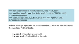
>>> from sklearn.metrics import precision_score, recall_score
>>> precision_score(y_train_5, y_train_pred) # == 4096 / (4096 + 1522)
0.7290850836596654
>>> recall_score(y_train_5, y_train_pred) # == 4096 / (4096 + 1325)
0.7555801512636044
it claims an image represents a 5, it is correct only 72.9% of the time. More over,
it only detects 75.6% of the 5s.
🔹 y_train_5 → True labels (ground truth).
🔹 y_train_pred → Predicted labels by the model

F1 score -combine precision and recall into a single metric called the F1 score.
• The F1 score is the harmonic mean of precision and recall
• Whereas the regular mean treats all values equally, the harmonic mean gives
much more weight to low values
in some contexts you mostly care about precision, and in other con texts you really care
about recall. For example, if you trained a classifier to detect videos that are safe for
kids, you would probably prefer a classifier that rejects many good videos (low recall) but
keeps only safe ones (high precision), rather than a classifier that has a much higher
recall but lets a few really bad videos show up in your product (in such cases, you may
even want to add a human pipeline to check the classifier’s video selection). On the
The harmonic mean is a type
useful when dealing with rate

Precision/Recall Trade-of
determines the minimum probability required for a positive prediction
There is often a tradeoff between precision and recall—improving one can lower the other.
🔹 If you increase precision, you become more selective, reducing false positives but
potentially missing some actual positives (lower recall).
🔹 If you increase recall, you try to catch as many positives as possible, but this may result in
more false positives (lower precision).
Example: Spam Email Detection
•If the spam filter is very strict (high precision), it only marks emails as spam when it’s very
sure, but it might miss some actual spam emails (low recall).
•If the spam filter flags too many emails as spam (high recall), it catches all spam emails, but
it might also wrongly mark some important emails as spam (low precision).
Adjusting the Tradeoff
•This balance is controlled using a decision threshold (e.g., probability score from a classifier).
•Lowering the threshold → More positives detected (higher recall, lower precision).
•Raising the threshold → Fewer false positives (higher precision, lower recall).

some real-world examples to help understand precision and recall:
1. Medical Diagnosis (Cancer Detection)
•Precision: Out of all patients diagnosed with cancer, how many actually have cancer?
•Recall: Out of all patients who truly have cancer, how many did the test detect?
• A high-precision test
. Fraud Detection (Credit Card Transactions)
•Precision: Out of all transactions flagged as fraud, how many were actually fraudulent?
•Recall: Out of all actual fraud cases, how many did the system detect?
• High precision avoids wrongly blocking legitimate transactions.
• High recall ensures most fraudulent transactions are caught, even if some false alarms
occur.
2. Autonomous Vehicles (Pedestrian Detection)
•Precision: Out of all detected pedestrians, how many were actually pedestrians?
•Recall: Out of all pedestrians on the road, how many did the system detect?
• High precision avoids unnecessary braking for non-pedestrians.
• High recall ensures all pedestrians are detected to prevent accidents.
3

. Job Resume Filtering (HR Systems)
•Precision: Out of all resumes selected for an interview, how many were actually qualified?
•Recall: Out of all qualified candidates, how many were selected for an interview?
• High precision avoids interviewing unqualified applicants.
• High recall ensures all strong candidates are considered.
4. Fake News Detection
•Precision: Out of all news articles flagged as fake, how many were actually fake?
•Recall: Out of all fake news articles available, how many were caught?
• High precision avoids wrongly marking real news as fake.
• High recall ensures most fake news is detected, even if some mistakes happen.
5. Voice Assistant (Wake Word Detection - e.g., "Hey Siri")
•Precision: Out of all times the assistant woke up, how many were actually triggered by "Hey Siri"?
•Recall: Out of all times the user said "Hey Siri", how many did the assistant recognize?
• High precision avoids waking up due to background noise.
• High recall ensures the assistant responds every time it's needed.

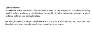
Decision Score
A decision score represents the confidence level or raw output of a machine learning
model before applying a classification threshold. It helps determine whether a given
instance belongs to a particular class.
decision_function() method, which returns a score for each instance, and then use any
threshold you want to make predictions based on those scores

The ROC Curve
• The receiver operating characteristic (ROC) curve is another
common tool used with binary classifiers.
• It is very similar to the precision/recall curve, but instead of plot
ting precision versus recall, the ROC curve plots the true positive
rate (TPR) (another name for recall) against the false positive rate
(FPR).
• The FPR is the ratio of negative instances that are incorrectly
classified as positive.

Multiclass Classification
Binary classifiers distinguish between two classes (Algorithms-Logistic Regression or
Support Vector Machine classifiers)
Multiclass classifiers (also called multinomial classifiers)
can distinguish between more than two classes.
algorithms- SGD classifiers, Random Forest classifiers,
and naive Bayes classifiers

There are various strategies that you can use to perform multiclass classification
with multiple binary classifiers.
1) one-versus-the-rest (OvR) strategy (also called one-versus-all).
• One way to create a system that can classify the digit images into 10 classes (from
0 to 9) is to train 10 binary classifiers, one for each digit (a 0-detector, a 1-detector,
a 2 detector, and so on).
• Then when we want to classify an image, you get the decision score from each
classifier for that image and you select the class whose classifier out puts the
highest score.
Example (MNIST = 10 classes):
•You train 10 classifiers:
•0 vs not-0
•1 vs not-1
...
•9 vs not-9

2) one-versus-one (OvO) strategy
• train a binary classifier for every pair of digits: one to distinguish 0s and 1s,
another to distinguish 0s and 2s, another for 1s and 2s, and so on. This is called the
one-versus-one (OvO) strategy. If there are N classes, you need to train N × (N –
1) / 2 classifiers.
• For the MNIST problem, this means training 45 binary classifiers! When you want
to classify an image, you have to run the image through all 45 classifiers and see
which class wins the most duels.
45 classifiers
️
🛠️How it works:
1.Train classifiers like:
•0 vs 1, 0 vs 2, ..., 8 vs 9

Support Vector Machine classifiers scale poorly with the size of the training set.
For these algorithms OvO is preferred
>>> from sklearn.svm import SVC
>>> svm_clf = SVC()
>>> svm_clf.fit(X_train, y_train)
>>> svm_clf.predict([some_digit])
array([5], dtype=uint8)
The decision_function() method in scikit-learn classifiers gives you the
confidence scores (also called decision values) instead of just the predicted
class.

If you call the decision_function() method, you will see that it
returns 10 scores per instance (instead of just 1). That’s one score
per class:
>>> some_digit_scores = svm_clf.decision_function([some_digit])
>>> some_digit_scores array([[ 2.92492871, 7.02307409, 3.93648529,
0.90117363, 5.96945908, 9.5 , 1.90718593, 8.02755089, -0.13202708,
4.94216947]])
The highest score is indeed the one corresponding to class 5:
>>> np.argmax(some_digit_scores)
5
>>> svm_clf.classes_ # unique class labels seen during training.
array([0, 1, 2, 3, 4, 5, 6, 7, 8, 9], dtype=uint8) # unsigned 8-bit integers
>>> svm_clf.classes_[5]
5

If you want to force Scikit-Learn to use one-versus-one or one-versus-the-
rest, you can use the OneVsOneClassifier or OneVsRestClassifier classes.
this code creates a multiclass classifier using the OvR strat egy, based on an
SVC
>>> from sklearn.multiclass import OneVsRestClassifier
>>> ovr_clf = OneVsRestClassifier(SVC())
>>> ovr_clf.fit(X_train, y_train)
>>> ovr_clf.predict([some_digit])
array([5], dtype=uint8)
>>> len(ovr_clf.estimators_) #trained 10 binary classifiers
10

Error Analysis
Once we have trained a promising model, the next step is to analyze what kinds of
mistakes it makes. This can help you uncover hidden patterns and guide your next
improvements.
1. A confusion matrix shows how often predictions matched actual labels. It’s your
first tool for spotting error patterns.
we need to make predictions using the cross_val_predict() function, then call the
confusion_matrix() function

>>> y_train_pred = cross_val_predict(sgd_clf, X_train_scaled, y_train, cv=3)
>>> conf_mx = confusion_matrix(y_train, y_train_pred)
>>> conf_mx

image representation of the confusion matrix, using Matplotlib’s matshow() function:

most images are on the main diago nal, which means that they were classified
correctly. The 5s look slightly darker than the other digits, which could mean that
there are fewer images of 5s in the dataset or that the classifier does not perform as
well on 5s as on other digits. In fact, you can verify that both are the case

Looking at this plot, it seems that your efforts should be spent on reducing the false 8s.
For example, you could try to gather more training data for digits that look like 8s (but are
not) so that the classifier can learn to distinguish them from real 8s.
Or you could engineer new features that would help the classifier—for example, writing
an algorithm to count the number of closed loops (e.g., 8 has two, 6 has one, 5 has none).
Or you could preprocess the images (e.g., using Scikit-Image, Pillow, or OpenCV) to make
some patterns, such as closed loops, stand out more.

Multilabel Classification
In some cases you may want your classifier to output multiple classes for each
instance.
Consider a face recognition classifier: what should it do if it recognizes several
people in the same picture? It should attach one tag per person it recognizes. Say
the classifier has been trained to recognize three faces, Alice, Bob, and Charlie.
Then when the classifier is shown a picture of Alice and Charlie, it should output
[1, 0, 1] (meaning “Alice yes, Bob no, Charlie yes”). Such a classification system
that outputs multiple binary tags is called a multilabel classification system.

Multioutput Classification
It is simply a generaliza tion of multilabel classification where each label can be
multiclass (i.e., it can have more than two possible values).
Key Difference:
•Multilabel classification: Each instance can have multiple binary labels (e.g., [1, 0, 1]).
•Multioutput classification: Each output label can have more than two classes (i.e.,
multiclass per output).

build a system that removes noise from images
It will take as input a noisy digit image, and it will (hopefully) output a clean digit image,
repre sented as an array of pixel intensities, just like the MNIST images. Notice that the
classifier’s output is multilabel (one label per pixel) and each label can have multiple
values (pixel intensity ranges from 0 to 255). It is thus an example of a multioutput
classification system.

Classification: MNIST, training a Binary classifier, performance measure, multiclass classification, error analysis, multi label classification, multi output classification.

Recommended

More Related Content

Similar to Classification: MNIST, training a Binary classifier, performance measure, multiclass classification, error analysis, multi label classification, multi output classification. (20)

More from BMS Institute of Technology and Management (15)

Recently uploaded (20)

Classification: MNIST, training a Binary classifier, performance measure, multiclass classification, error analysis, multi label classification, multi output classification.