Data Structure And Algorithms for Computer Science

SYLLABUS
 Terminologies,
 Representation of binary Trees: Using Arrays and linked lists,
 Binary Tree Traversals: Recursive and Non-Recursive
techniques,
 Threaded Binary trees,
 Binary search tree operations: Traversal, Searching, Inserting
and Deleting elements;
 AVL search tree operations: Insertion and Deletion,
 m-way search tree, Searching Insertion and Deletion in an m-
way search tree,
 B- tree Searching, Insertion and Deletion in a B- tree,
 Heap Sort.
2

Definition of Tree
• A tree is a finite set of one or more nodes
such that:
• There is a specially designated node called
the root.
• The remaining nodes are partitioned into n>=0 disjoint
sets T1, ..., Tn, where each of these sets is a tree.
• We call T1, ..., Tn the subtrees of the root.
3

TREE – TERMINOLOGY
Root : The basic node of all nodes in the tree.
 Child : a successor node connected to a node is called child. ( B
and C are child nodes to the node A, Like that D and E are child
nodes to the node B. )
 Parent : a node is said to be parent node to all its child nodes. ( A
is parent node to B,C and B is parent node to the nodes D and F).
 Leaf : a node that has no child nodes. ( D, E and F are Leaf nodes
)
 Siblings : Two nodes are siblings if they are children to the same
parent node.
Ancestor : a node which is parent of parent node ( A is ancestor
node to D,E and F ).
 Descendent : a node which is child of child node ( D, E and F are
descendent nodes of node A )
Degree : The number of sub tree of a node. A binary tree is degree
2.
4

TREE – TERMINOLOGY
Level : The distance of a node from the root node,
The root is at level – 0,( B and C are at Level 1 and D,
E, F have Level 2.
Depth or height: of a tree is the maximum number
of nodes in a branch of T. this turns out to be 1 more
than the largest level number of T.
Edge: The line drawn from a node N of T to a
successor is called an edge.
Path: A sequence of consecutive edges is called
path.
A forest is a disjoint union of trees.
5

BINARY TREE
A binary tree is a finite set of elements that is either empty or is
partitioned into three disjoint subsets.
- The first subset contains a single element called the root of the
tree.
- The other two subsets are themselves binary trees, called the left
and right subtrees of the original tree. A left or right subtree can be
empty. Each element of a tree is called a node of the tree.
B
G
E
D
I
H
F
c
A Binary tree
8

STRUCTURES THAT ARE NOT BINARY TREES
9

TYPES OF BINARY TREE
1. Strictly binary trees
2. Complete binary tree
3. Extended binary tree
10

STRICTLY BINARY TREES
•If every non-leaf node in a binary tree must have two subtree
left and right sub-trees, the tree is called a strictly binary tree.
•A strictly binary tree with n leaves always contains 2n -1
nodes.
•Here, B,E,F,G are leaf nodes. So n=4, No. of nodes=2*4-1=7
B
D
G
F
E
C
A
11

COMPLETE BINARY TREE
The tree is said to be complete binary tree if all its levels, except
possibly the last, have the maximum number of possible nodes
and if all the nodes at last level appear as far left as possible.
Maximum number of nodes at any level r =2r
Eq:- at level 0 maximum number of nodes=2º=1
At level 2 maximum number of nodes=2²=4 and so on.
.
12

COMPLETE BINARY TREE
Suppose given a complete binary tree having 26 nodes. We are labeling the
nodes from 1 to 26.
Left child of node k=2*K
Right child of node k=2*K+1
Parent of node K=[K/2]
Depth of complete binary tree Tn with n node
D n = [log 2n +1]
13

FULL BINARY TREE VS COMPLETE BINARY
TREE
14

FULL VS. COMPLETE BINARY TREE
15

EXTENDED BINARY TREE
•An extended binary tree is a transformation of any binary tree
into a complete binary tree. This transformation consists of
replacing every null subtree of the original tree with ‘special
nodes.'
•The nodes from the original tree are then internal nodes, while
the ``special nodes'' are external nodes.
•For instance, consider the following binary tree in fig(a). Fig
(b) is the extended binary tree.
•Empty circles represent internal nodes, and filled circles
represent external nodes. Every internal node in the extended
tree has exactly two children, and every external node is a leaf.
The result is a complete binary tree.
16

REPRESENTATION OF BINARY TREES IN MEMORY
.
Array Representation
Linked Representation
18

ARRAY REPRESENTATION
.
• Tree Nodes are stored in the array.
• Root node is stored at index ‘0’
• If a node is at a location ‘i’, then its
left child is located at 2 * i + 1
right child is located at 2 * i + 2
• This storage is efficient when it is a complete binary tree,
because a lot of memory is wasted.
19

EXAMPLE 2
Disadvantages
(1) waste space
(2) insertion/deletion
problem
21

LINKED REPRESENTATION
•If a binary tree is not complete , a better choice for storing
it is to use a linked representation.
•It uses three array INFO, RIGHT, LEFT, and a pointer
variable ROOT as follows.
•First of all, each node N of tree T will correspond to a
location K such that:
•INFO[K] contains the data at node N.
•RIGHT[K] contains the location of the right child of node
N.
•LEFT[K] contains the location of the left child of node N.
•ROOT will contain the location of the root R of T.
22

Linked Representation
struct node {
int info;
struct node *left;
struct node *right;
};
info
left right
info
left right
23

ROOT
A
B x C x
x D x E x
x F x
24

1
2
3
4
5
6
7
8
9
10
B
C
D
E
A 3 6
8 9
X X
X
7 X
X
1
ROOT
F
4
5
X X
2
AVAIL
25

TRAVERSING A BINARY TREE
Three methods:
1. inorder
2. preorder
3. postorder
Preorder
1. Visit the root
2. Traverse the left subtree in preorder
3. Traverse the right subtree in preorder
Root-left-right
9
3
4
14
18
15
20
7 16
17
5
Postorder
1. Traverse the left subtree in postorder
2. Traverse the right subtree in postorder
3. Visit the root
Left-right-root
Inorder
1. Traverse the left subtree in inorder
2. Visit the root
3. Traverse the right subtree in inorder
Left-root-right
26

Preorder
1. Visit the root
preorder: ABDGCEHIF
Postorder
3. Visit the root
postorder: GDBHIEFCA
D
B
A
F
C
E
G
I
H
Inorder
2. Visit the root
inorder: DGBAHEICF
28

Preorder
1. Visit the root
preorder: ABCEIFJDGHKL
Inorder
2. Visit the root
inorder: EICFJBGDKHLA
Postorder
3. Visit the root
postorder: IEJFCGKLHDBA
C
B
A
L
H
D
K
G
E
I
F
J
29

APPLY EACH TRAVERSAL IN BINARY
TREE
30
PREORDER: ABDCEFG
INORDER: BDAECGF
POSTORDER: DBEGFCA

TRAVERSING
There are two solution for traversing
•Recursive
•Non-recursive
31

RECURSIVE TRAVERSAL OF BINARY TREE
32

INORDER
inorder (node *root)
{
if (root != NULL)
{
inorder (left[root]);
print (info[root]);
inorder (right[root]);
}
}
33

PREORDER
preorder (node *root)
{
if (root != NULL)
{
print (info[root]);
preorder (left[root]);
preorder (right[root]);
}
}
34

POST ORDER
postorder (node *root)
{
if (root != NULL)
{
postorder (left[root]);
postorder (right[root]);
print (info[root]);
}
}
35

NON-RECURSIVE TRAVERSAL OF BINARY
TREE
36

INORDER TRAVERSAL
1) Create an empty stack S.
2) Initialize current node as root
3) Push the current node to S and
set current =current->left until current is NULL
4) If current is NULL and stack is not empty then
a) Pop the top item from stack.
b) Print the popped item, set current = current->right
c) Go to step 3.
5) If current is NULL and stack is empty then we are done.
37

In non recursive traversing, stack is used to store the nodes which has to
be visited later.
1.Set Top := 0
2. P= Root.
3. Repeat step 4 to 10 while (P ≠ NULL)
4. Repeat Steps 5 to 6 while (P ≠ NULL)
5. Push(Stack,P)
6. P=Left[P]
[End of Step 4 while loop.]
7. IF(Stack is non empty)
8. P=Pop(Stack)
9. Print P
10. P=Right[P]
[End of If structure.]
11.Stop
INORDER TRAVERSAL
struct node {
int info;
struct node *left;
struct node *right;
};
38

PREORDER TRAVERSAL
1.P= Root.
2. Push(Stack,P)
3. Repeat step 4 to 9 while (stack is non empty)
4. P=Pop(Stack)
5. If (Right[P]!=Null)
6. Push(Stack, Right[P])
7. If (Left[P]!=Null)
8. Push(Stack, Left[P])
9. Print Info[P]
10.Stop
struct node {
int info;
struct node *left;
struct node *right;
};
40

POSTORDER TRAVERSAL
1.P= Root.
2. Push(Stack, Root)
3. Repeat step 4 to 13 while (stack is non empty)
4. P=Stack[Top]
5. If (Left[P]!=Null && Visited[Left[P]]==FALSE)
6. Push(Stack, Left[P])
7. Else
8.If(Right[P]!=Null && Visited[Right[P]]==FALSE)
9. Push(Stack, Right[P])
10. Else
11. Pop(Stack)
12. Print Info[P]
13.visited[P]=TRUE
[End of if]
[End of while]
14.Stop
#define BOOL int
struct node {
int info;
struct node *left;
struct node *right;
BOOL visited;
};
42

CREATION OF BINARY TREE FROM PREORDER
AND INORDER TRAVERSALS
Step 1: Scan the preorder traversal from left to right.
Step 2: For each node scanned locate its position in
inorder traversal. Let the scanned node x.
Step 3: The node x preceding x in inorder from its left
subtree and nodes succeeding it from right subtree.
Step 4: Repeat step 1 for each symbol in the
preorder.
44

CONSTRUCT TREE FROM GIVEN INORDER AND
PREORDER TRAVERSALS
 Let us consider the below traversals:
 Inorder sequence: D B E A F C
Preorder sequence: A B D E C F
Solution: In a Preorder sequence, leftmost element is
the root of the tree. So we know ‘A’ is root for given
sequences. By searching ‘A’ in Inorder sequence,
we can find out all elements on left side of ‘A’ are in
left subtree and elements on right are in right
subtree. So we know below structure now.
45

 We recursively follow above steps and get the
following tree.
46

 Inorder sequence: CAFDGHB
 Preorder sequence: DACFBGH
CONSTRUCT TREE FROM GIVEN INORDER AND
PREORDER TRAVERSALS
47

CONSTRUCT THE TREE FROM ITS GIVEN
PREORDER AND POSTORDER
 Construct the tree from its given preorder and
postorder traversal. Explain the steps involved.
Preorder: A B D G H K C E F
Postorder: G K H D B E F C A
49

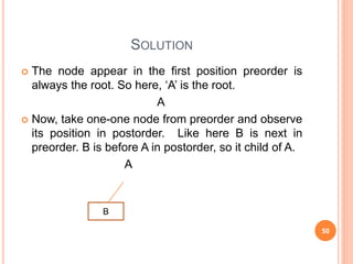
SOLUTION
 The node appear in the first position preorder is
always the root. So here, ‘A’ is the root.
A
 Now, take one-one node from preorder and observe
its position in postorder. Like here B is next in
preorder. B is before A in postorder, so it child of A.
A
B
50

 Next node in preorder is D. D is before B in postorder.
 Next node in preorder is G. G is before D in postorder.
51

 Next node in preorder is H. H is before D in postorder.
But D is already having a left child. H will become right
child of D.
H
•Next node in preorder is K. K is before H in postorder.
52

 Next node in preorder is C . C is before A in
postorder. But A is already having a left child. C will
become right child of A.
53

 Next node in preorder is E . E is before F in
postorder. EF is before C in postorder.
F
E
54

HEADER NODES
 Suppose a binary tree T is maintained in memory by means of a
linked representation. Sometimes an extra, special node, called a
header node, is added to the beginning of T.
 When this extra node is used, the tree pointer variable, which we call
HEAD, will point to the header node, and the left pointer of the
header node will point to the root of T.
55

Threaded Binary Trees
• Too many null pointers in current representation of binary trees
n: number of nodes
number of non-null links: n-1
total links: 2n
null links: 2n-(n-1)=n+1
• This space may be more efficiently used by replacing the null
entries by some other type of information.
• We will replace null entries by special pointers which point to
nodes higher in the tree.
• These special pointers are called “threads”, and binary trees
with such pointers are called threaded tree.
• The threads in a binary tree are usually indicated by dotted lines.
56

THREADED BINARY TREES
Tree can be threaded using
• One way threading:
i. Right-in –threaded: a thread will appear in the
RIGHT Null field of each node and will point to
the successor of that node under inorder traversal.
ii. Left-in-threaded: a thread will appear in the LEFT
Null field of each node and will point to the
predecessor of that node under inorder traversal.
• Two way threading(fully threaded tree): both left and
right Null pointers can be used to point to predecessor
and successor of that node under inorder traversal.
57

RIGHT-IN –THREADED
Inorder:FBHGADCE
58

LEFT-IN-THREADED
Inorder:FBHGADCE
59

BINARY SEARCH TREES (BST)
 A binary search tree T is a binary tree which is
either empty or each node of the tree contains a
key that satisfies the following conditions:
i. All keys in the left of the root are less than the key in
the root.
ii. All keys in the right of the root are greater than the
key in the root.
iii. The left and right subtree of the root are also binary
search trees.
61

EXAMPLES
20 35 48 85
78
50
53
45
12
75
30
80
20
12
15
5
10
63

ADVANTAGES & DISADVANTAGES OF BINARY SEARCH TREE
Advantages
i. Stores keys in the nodes in a way that searching, insertion and
deletion can be done efficiently.
ii. Simple Implementation
iii. Nodes in tree are dynamic
Disadvantages
i. The shape of the tree depends on the order of insertions, and it can
be degenerated.
ii. When inserting or searching for an element, the key of each visited
node has to be compared with the key of the element to be
inserted/found.
iii. Keys in the tree may be long and the run time may increase.
64

OPERATIONS ON BINARY SEARCH TREE
•Traverse
•Searching
•Inserting
•Deleting
65

TRAVERSE
 The inorder, preorder and postorder algorithms will
remain same as binary tree. When a BST is
traversed in inorder, the elements are printed in
ascending order.
 Example: inorder: 5, 10, 12, 15,20
66

SEARCHING
 The search will start from the root X.
 K is the key value which we are searching in the
tree.
TREE_SEARCH(X,K)
1. If (X==NULL) or K=Info[X]
return X
2. If K < Info[X]
return TREE_SEARCH(Left[X], K)
3. Else
return TREE_SEARCH(Right[X], K)
67

INSERTION
 The operations of insertion and deletion change the
dynamic set represented by a binary search tree.
 Before the node can be inserted into a BST, the
position of the new node must be determined.
 The insert operation will insert a node to a tree and
the new node will become leaf node.
 This is to ensure that after the insertion, the BST
characteristics is still maintained.
69

Insertion(T, Z) //T Binary Search Tree, Z new node
1. y=NULL
2. x=root
3. While x ≠ NULL
4. do y=x
5. If info[z] < info[x]
6. then x=left[x]
7. Else x=right[x]
[End while]
8. parent[z]=y
9. If y==NULL //tree was empty
10. then root=z
11. Else if info[z] < info[y]
12. then left[y]=z
13. Else right[y]=z
14. Stop 70

CONSTRUCT A BINARY SEARCH TREE
71

CONSTRUCT BINARY SEARCH TREE
How can you construct binary search tree with the
following element sequence.
40,60,50,33,55,11
72
60
33
11 50
55
40

CONSTRUCT BINARY SEARCH TREE
How can you construct binary search tree with the
following element sequence.
44,22,77,33,55,99,88
73
77
22
33 55 99
44
88

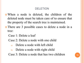
DELETION
 When a node is deleted, the children of the
deleted node must be taken care of to ensure that
the property of the search tree is maintained.
 There are 3 possible cases to delete a node in a
tree:
Case 1: Delete a leaf
Case 2: Delete a node with one child
a) Delete a node with left child
b) Delete a node with right child
Case 3: Delete a node that has two children 74

Delete(T,x) //delete a node with info x from a tree T.
First search a node with info x. let there is node p with
info x and q be its parent. If no such p exists there,
x is not present so no deletion is possible.
Case 1: Let p be a leaf node
If (q==null) and root=p then set root=null
Else
if (left[q]==p) then left[q]=null
else right[q]=null
75

Case 2(a): let p have only left child
If (q==null) then root=left[p]
Else
If (left[q]==p) then left[q]=left[p]
else right[q]=left[p]
76

Case 2(b): let p have only right child
If (q==null) then root=right[p]
else
If (left[q]==p) then left[q]=right[p]
else right[q]=right[p]
78

Case 3: p has both left and right child,
 replace the node's value with the min value in the
right subtree
 delete the min node in the right subtree
79

BALANCE FACTOR (BF)
 For each node the balanced factor (bf) is defined as
bf(N)= height of left subtree of N – height of right subtree of N
80

AVL (HEIGHT-BALANCED TREES)
 It is named after their inventors, Adelson, Velskii and
Landis.
 An AVL tree is a binary search tree which has the
following properties:
 The height of the left and right subtrees of the root
differs by atmost 1
 The left and right subtrees of the root are again AVL
trees
 Node balance factor of +1 if node left subtree is high,
0 if node both subtree are at equal hight and -1 is node
right subtree is high.
81

PERFECTLY BALANCED BINARY TREE
82

INSERTION ALGORITHM
 Insert(T,x)
Step 1: Insert x into T using BST insertion algorithm.
Step 2: Recalculate the balance factor for each node.
Step 3: Backtrack towards root following the path of
insertion. Stop at first node which does not have a
balance factor belonging to (0,1,-1). If no such node
is found , stop and insertion is over. If one such
node is found, then go for rotation.
85

SINGLE & DOUBLE ROTATIONS
 Single
 LL and RR
 Double
 LR:LR is RR followed by LL
 RL:RL is LL followed by RR
86

AVL ROTATION
In order to balance a tree, there are four types of
rotations
 LL Rotation: inserted node is added to the left
subtree of the left child of the unbalanced node.
 RR Rotation: inserted node is added to the right
subtree of the right child of the unbalanced node.
 LR Rotation: inserted node is added to the right
subtree of the left child of the unbalanced node.
 RL Rotation: inserted node is added to the left
subtree of the right child of the unbalanced node.
87

LL ROTATION EXAMPLE
89
Insert node 10 in this tree

CONSTRUCT AVL TREE
96
Insert the following nodes in an AVL tree:
40, 30,20, 60,50, 80,15,28,25

AVL TREE ROTATIONS
97
40, 30,20, 60,50, 80,15,28,25

AVL TREE ROTATIONS
98
40, 30,20, 60,50, 80,15,28,25

AVL TREE ROTATIONS
99
40, 30,20, 60,50, 80,15,28,25

AVL TREE ROTATIONS
100
40, 30,20, 60,50, 80,15,28,25

AVL TREE ROTATIONS
101
40, 30,20, 60,50, 80,15,28,25

AVL TREE ROTATIONS
102
40, 30,20, 60,50, 80,15,28,25

AVL TREE ROTATIONS
103
40, 30,20, 60,50, 80,15,28,25

AVL TREE ROTATIONS
104
40, 30,20, 60,50, 80,15,28,25

DELETION IN AN AVL TREES
The sequence of steps to be followed in deleting a node
from an AVL tree is as follows:
1. Initially, the AVL tree is searched to find the node to be
deleted.
2. The procedure used to delete a node in an AVL tree is
the same as deleting the node in the BST.
3. After deletion of the node, check the balance factor of
each node.
4. Rebalance the AVL tree if the tree is unbalanced. For
this, AVL rotations are used.
105

 On deletion of a node X from the AVL tree, let A be the
closest ancestor node on the path from X to the root
node, with a balance factor of +2 or -2. To restore
balance the rotation is first classified as L or R depending
on whether the deletion occurred on the left or right
subtree of A.
 B is the root of the left or right subtree of A. Now
depending upon the value of balance factor of B, the R
or L rotation is further classified as R0, R1 and R-1 or
L0, L1, L-1.
106

TYPES OF ROTATION
R0 (LL) L0 (RR)
R1 (LL) L1 (RR)
R-1(LR) L-1(RL)
107

R0 ROTATION
108
When balance factor of B is 0 and B is the root of left
subtree of A. R0 rotation is used.(R0 rotation are similar
to LL).

R1 ROTATION
111
When balance factor of B is 1 and B is the root of left
subtree of A. R1 rotation is used. (R1 rotation are
similar to LL).

R(-1) ROTATION
113
When balance factor of B is -1 and B is the root of left subtree
of A. R(-1) rotation is used. (R(-1) rotation are similar to
LR).

EXAMPLE L0 ROTATION
114
When balance factor of B is 0 and B is the root of right subtree
of A. L0 rotation is used. (L0 rotation are similar to RR).

L1 ROTATION
115
When balance factor of B is 1 and B is the root of right
subtree of A. L1 rotation is used. (L1 rotation are
similar to RR ).

116
Insert the following keys in order shown to construct an
AVL tree 10,20,30,40,50. delete the last two keys in the
order of LIFO.

118
Advantages
1. Search is O(log N) since AVL trees are always balanced.
2. Insertion and deletions are also O(logn)
3. The height balancing adds no more than a constant factor to the speed of
insertion.
Disadvantages
1. Difficult to program & debug; more space for balance factor.
2. Asymptotically faster but rebalancing costs time.
3. Most large searches are done in database systems on disk and use other
structures (e.g. B-trees).
Pros and Cons of AVL Trees

M-way search tree
Searching , Insertion and Deletion
119

DEFINITION
 A multi-way tree of order m (or an m-way tree) is a tree T in
which
i. Each nodes hold between 1 to m-1 distinct keys and each
node has, at most m child nodes.
ii. In a node, values are stored in ascending order:K1 < K2 <
... < Km-1
iii. The subtrees are placed between adjacent values: each
value has a left and right subtree.
 ki right subtree = ki+1 left subtree.
 All the values in ki left subtree are < ki
 All the values in ki right subtree are > ki
iv. Each of the subtree Ai, 1≤i≤m are also m-way search trees.
120

ALGORITHM FOR SEARCHING FOR A
VALUE IN AN M-WAY SEARCH TREE
1. If X < K1, recursively search for X in K1 's left
subtree.
2. If X > Km-1, recursively search for X in Km-1 's right
subtree.
3. If X= Ki, for some i, then we are done (X has
been found).
4. The only remaining possibility is that, for some i,
Ki < X < Ki+1. In this case recursively search for X
in the subtree that is in between Ki and Ki+1
122

INSERTION IN AN M-WAY SEARCH TREE
 To insert a new element into an m-way search tree
we proceed in the same way as one would in order
to search for the element.
 To insert 6 into the 5-way search tree, we proceed
to search for 6 and find that we fall off the tree at
the node [7,12] with the first child node showing a
null pointer.
 Since the node has only two keys and a 5-key
search tree can accommodate up to 4 keys in a
node, 6 is inserted into the node as [6,7,12].
 But to insert 146, the node [148,151,172,186] is
already full, hence we open a new child node and
insert 146 into it.
123

INSERTION IN AN 5-WAY SEARCH TREE
124

DELETION IN AN M-WAY SEARCH TREE
 Let K be a key to be deleted from the m-way search
tree. To delete the key we proceed as one would to
search for the key.
 Let the node accommodating the key as shown in figure
125

DELETION IN AN M-WAY SEARCH TREE
There are four case
Case 1: if (Ai = Aj = NULL) then delete K.
Case 2: if (Ai ≠ NULL, Aj = NULL) then choose the largest of the key
element K’ in the child node pointed to by Ai, delete the key K’ and
replace K by K’ . Obviously deletion of K’ may call for subsequent
replacements and therefore deletions in a similar manner, to enable
the key K’ move up the tree.
Case 3: if (Ai = NULL, Aj ≠ NULL) then choose the smallest of the
key element K’’ in the child node pointed to by Aj, delete the key K’’
and replace K by K’’ . Again deletion of K’’ may trigger subsequent
replacements and deletions to enable K’’ move up the tree.
Case 4: if (Ai ≠ NULL, Aj ≠ NULL) then choose either the largest of
the key element K’ in the child node pointed to by Ai, or the smallest
of the key elements K’’ from the subtree pointed to by Aj, to
replace K. To move K’ or K’’ up the tree it may call for subsequent
replacements and deletions. 126

CASE 1
 To delete 151, we search for 151 and observe that in the leaf node
[148,151, 172, 186] where it is present, both its left subtree pointer
and right subtree pointer are such that ((Ai = Aj = NULL).
 We therefore simply delete 151 and the node becomes [148, 172,
186]. Deletion of 92 also follows the same process.
127

CASE 2
 To delete 12 (in the figure of slide 120), we find the
node [7,12] accommodates 12 and key satisfies (Ai ≠
NULL, Aj = NULL). Hence we choose the largest of the
keys from the node pointed to by Ai 10 and replace 12 with
10.
128

CASE 3
 To delete 262 (in the figure of slide 120, we find its left and right
subtree pointers Ai and Aj respectively, are such that (Ai = NULL,
Aj ≠ NULL).
 Hence we choose the smallest element 272 from the child node [272,
286, 300], delete 272 and replace 262 with 272. to delete 272 the
deletion procedure needs to be observed again.
129

CASE 4
 To delete 198 (in the figure of slide 120, we find its left and right
subtree pointers Ai and Aj respectively, are such that (Ai ≠ NULL,
Aj ≠ NULL).
 Hence we choose the largest element 141 from the child node [80,
92, 198], delete 141 and replace 198 with 141. in place of 141, 148
will come.
130

INTRODUCTION
 M-way search trees have the advantages of
minimizing file accesses due to their restricted
height.
 However it is essential that the height of the tree be
kept as low as possible and therefore there arises
the need to maintain balanced m-way search trees.
Such a balanced m-way search tree is what is
defined as a B-tree.
132

DEFINITION OF A B-TREE
A B-tree of order m is an m-way search tree in which:
1. the root has at least two child nodes and at most m
child nodes.
2. all internal (non-leaf) nodes except the root have at
least m / 2 (ceil) child nodes and at most m child
nodes.
3. the number of keys in each internal (non-leaf) node is
one less than the number of its child and these keys
partition the keys in the subtree of the node in a
manner similar to that of m-way search trees.
4. all leaf nodes are on the same level.
133

SEARCHING IN A B-TREE
 Searching for a key in a B-tree is similar to one an
m-way search tree. The number of accesses
depends on the height h of the B-tree.
135

INSERTING INTO A B-TREE
The insertion of a key in a B-tree proceeds as if one were
searching for the key in the tree. Then the key is inserted
according to the following procedure:
Case 1: if the leaf node in which the key is to be inserted is
not full, then the insertion is done in the node. A node is
said to be full if it contains a maximum of (m-1) keys,
given the order of the B-tree to be m.
Case 2: if the node were to be full, then insert the key in
order into the existing set of keys in the node, split the
node at its median into two nodes at the same level,
pushing the median element in the parent node if it is not
full.
136

INSERTION INTO A B-TREE
137
Consider the B-tree of order 5 shown below. Insert the elements 4,5, 58, 6 in
The order given.

139
 Suppose we start with an empty B-tree and keys arrive in the
following order:1 12 8 2 25 6 14 28 17 7 52 16 48 68
3 26 29 53 55 45
 We want to construct a B-tree of order 5
 The first four items go into the root:
 To put the fifth item in the root would violate condition
 Therefore, when 25 arrives, pick the middle key to make a new
root
CONSTRUCTING A B-TREE
1 2 8 12

140
CONSTRUCTING A B-TREE (CONTD.)
1 2
8
12 25
6, 14, 28 get added to the leaf nodes:
1 2
8
12 14
6 25 28

141
Adding 17 to the right leaf node would over-fill it, so we take the
middle key, promote it (to the root) and split the leaf
8 17
12 14 25 28
1 2 6
7, 52, 16, 48 get added to the leaf nodes
8 17
12 14 25 28
1 2 6 16 48 52
7

142
Adding 68 causes us to split the right most leaf, promoting 48 to the
root, and adding 3 causes us to split the left most leaf, promoting 3
to the root; 26, 29, 53, 55 then go into the leaves
3 8 17 48
52 53 55 68
25 26 28 29
1 2 6 7 12 14 16
Adding 45 causes a split of 25 26 28 29
and promoting 28 to the root then causes the root to split

143
17
3 8 28 48
1 2 6 7 12 14 16 52 53 55 68
25 26 29 45

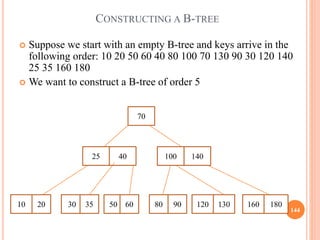
144
 Suppose we start with an empty B-tree and keys arrive in the
following order: 10 20 50 60 40 80 100 70 130 90 30 120 140
25 35 160 180
 We want to construct a B-tree of order 5
CONSTRUCTING A B-TREE
70
25 40 100 140
20
10 30 35 50 60 80 90 120 130 160 180

145
DELETION FROM A B-TREE
1. If the key is already in a leaf node, and removing it doesn’t cause
that leaf node to have too few keys, then simply remove the key to
be deleted.
2. If the key is not in a leaf then it is guaranteed that its predecessor or
successor will be in a leaf -- in this case we can delete the key and
promote the predecessor or successor key to the non-leaf deleted
key’s position.
 If (1) or (2) lead to a leaf node containing less than the minimum
number of keys then we have to look at the siblings immediately
adjacent to the leaf :
3. if one of them has more than the min. number of keys then we
can promote one of its keys to the parent and take the parent key
into our lacking leaf
4. if neither of them has more than the min. number of keys then the
lacking leaf and one of its neighbours can be combined with their
shared parent (the opposite of promoting a key) and the new leaf
will have the correct number of keys; if this step leave the parent
with too few keys then we repeat the process up to the root itself,
if required

146
CASE #1: SIMPLE LEAF DELETION
12 29 52
2 7 9 15 22 56 69 72
31 43
Delete 2: Since there are enough
keys in the node, just delete it
Assuming a 5-way
B-Tree, as before...

147
CASE #2: SIMPLE NON-LEAF DELETION
12 29 52
7 9 15 22 56 69 72
31 43
Delete 52
Borrow the predecessor
or (in this case) successor
56

148
CASE #4: TOO FEW KEYS IN NODE AND ITS
SIBLINGS
12 29 56
7 9 15 22 69 72
31 43
Delete 72
Too few keys!
Join back together

149
CASE #4: TOO FEW KEYS IN NODE AND ITS
SIBLINGS
12 29
7 9 15 22 69
56
31 43

150
CASE #3: ENOUGH SIBLINGS
12 29
7 9 15 22 69
56
31 43
Delete 22
Demote root key and
promote leaf key

151
CASE #3: ENOUGH SIBLINGS
12
29
7 9 15
31
69
56
43

152
Consider the B-tree of order 5 shown below. Delete the keys 95, 226 , 221
and 70.

DELETION IN A B-TREE
 The deletion of key 95 is simple and straight since the leaf node has
more than the minimum number of elements.
 To delete 226, the internal node has only the minimum number of
elements and hence borrows the immediate successor viz., 300 from
the leaf node which has more than the number of elements.
 Deletion of 221 calls for the hauling of key 440 to the parent node
and pulling down of 300 to take the place of the deleted entry in the
leaf.
 Lastly the deletion of 70 is a little more involved in process. Since
none of the adjacent leaf nodes can afford lending a key, two of the
leaf nodes are combined with the intervening element from the
parent to form a new leaf node, viz,[32,44,85, 81] leaving 86 alone
in the parent node.
 This is not possible since the parent node is now running low on its
minimum number of elements. Hence we once again proceed to
combine the adjacent sibling nodes of this yields the
node[86,110,120,440] which is the new root.
153

EXAMPLE
154
 On the B-tree of order 3 given below, perform the
following operations in the order of their
appearance:
Insert 75, 57 delete 35,65

ALGORITHM TO FIND THE NO. OF LEAF NODES
IN THE BINARY TREE
get_leaf_node(node)
1. If node==Null then
Return 0
2. If left[node]=Null && right[node]==Null then
Return 1
3. Else
Return get_leaf_node(left[node])+
get_leaf_node(right[node])
156

A DATA STRUCTURE HEAP
 A heap is an array object that can be viewed as a
nearly complete binary tree.
3
5
2 4 1
6
6 5 3 2 4 1
1
2 3
4 5 6
158

159
ARRAY REPRESENTATION OF HEAPS
 A heap can be stored as an array
A.
 Root of tree is A[1]
 Left child of A[i] = A[2i]
 Right child of A[i] = A[2i + 1]
 Parent of A[i] = A[ i/2 ]

160
HEAP TYPES
 Max-heaps (largest element at root), have the max-heap
property:
 for all nodes i, excluding the root:
A[PARENT(i)] ≥ A[i]
 Min-heaps (smallest element at root), have the min-heap
property:
 for all nodes i, excluding the root:
A[PARENT(i)] ≤ A[i]

161
ADDING/DELETING NODES
 New nodes are always inserted at the bottom level (left to right)
 Nodes are removed from the bottom level (right to left)

162
OPERATIONS ON HEAPS
 Maintain/Restore the max-heap property
 MAX-HEAPIFY
 Create a max-heap from an unordered array
 BUILD-MAX-HEAP
 Sort an array in place
 HEAPSORT

163
MAINTAINING THE HEAP PROPERTY
 Suppose a node is smaller than a child
 Left and Right subtrees of i are max-heaps
 To eliminate the violation:
 Exchange with larger child
 Move down the tree
 Continue until node is not smaller than children

164
EXAMPLE
MAX-HEAPIFY(A, 2, 10)
A[2] violates the heap property
A[2]  A[4]
A[4] violates the heap property
A[4]  A[9]
Heap property restored

165
MAINTAINING THE HEAP PROPERTY
 Assumptions:
 Left and Right
subtrees of i are
max-heaps
 A[i] may be
smaller than its
children
Alg: MAX-HEAPIFY(A, i, n)
1. l ← LEFT(i)
2. r ← RIGHT(i)
3. if l ≤ n and A[l] > A[i]
4. then largest ←l
5. else largest ←i
6. if r ≤ n and A[r] > A[largest]
7. then largest ←r
8. if largest  i
9. then exchange A[i] ↔ A[largest]
10. MAX-HEAPIFY(A, largest, n)

166
BUILDING A HEAP
Alg: BUILD-MAX-HEAP(A)
1. n = length[A]
2. for i ← n/2 downto 1
3. do MAX-HEAPIFY(A, i, n)
 Convert an array A[1 … n] into a max-heap (n = length[A])
 The elements in the subarray A[(n/2+1) .. n] are leaves
 Apply MAX-HEAPIFY on elements between 1 and n/2
2
14 8
1
16
7
4
3
9 10
1
2 3
4 5 6 7
8 9 10
4 1 3 2 16 9 10 14 8 7
A:

167
EXAMPLE: A 4 1 3 2 16 9 10 14 8 7
2
14 8
1
16
7
4
3
9 10
1
2 3
4 5 6 7
8 9 10
14
2 8
1
16
7
4
10
9 3
1
2 3
4 5 6 7
8 9 10
2
14 8
1
16
7
4
3
9 10
1
2 3
4 5 6 7
8 9 10
14
2 8
1
16
7
4
3
9 10
1
2 3
4 5 6 7
8 9 10
14
2 8
16
7
1
4
10
9 3
1
2 3
4 5 6 7
8 9 10
8
2 4
14
7
1
16
10
9 3
1
2 3
4 5 6 7
8 9 10
i = 5 i = 4 i = 3
i = 2 i = 1

168
HEAP SORT
 Goal:
 Sort an array using heap representations
 Idea:
 Build a max-heap from the array
 Swap the root (the maximum element) with the last element
in the array
 “Discard” this last node by decreasing the heap size
 Call MAX-HEAPIFY on the new root
 Repeat this process until only one node remains

169
EXAMPLE: A=[7, 4, 3, 1, 2]
MAX-HEAPIFY(A, 1, 4) MAX-HEAPIFY(A, 1, 3) MAX-HEAPIFY(A, 1, 2)
MAX-HEAPIFY(A, 1, 1)

170
ALG: HEAPSORT(A)
1. BUILD-MAX-HEAP(A)
2. for i ← length[A] downto 2
3. do exchange A[1] ↔ A[i]
4. MAX-HEAPIFY(A, 1, i - 1)

Data Structure And Algorithms for Computer Science

Recommended

More Related Content

Similar to Data Structure And Algorithms for Computer Science (20)

Recently uploaded (20)

Data Structure And Algorithms for Computer Science