Digital image processing using matlab: basic transformations, filters and operators
9 likes7,778 views

This document provides code solutions in Matlab for image processing homework assignments. It includes code to perform: 1. Basic grayscale transformations like negative, log, power-law, and piecewise linear on various images. 2. Histogram processing techniques like equalization and subtraction on images. 3. Smoothing and sharpening filters like averaging, median, Laplacian, and Sobel gradient filters to reduce noise and enhance edges. 4. Detailed explanations and examples are given for each transformation and filtering technique along with input and output images. The code utilizes various Matlab functions to perform the image processing tasks in a concise manner.
1 of 20
Downloaded 324 times
![NATIONAL CHENG KUNG UNIVERSITY
Inst. of Manufacturing Information & Systems
DIGITAL IMAGE PROCESSING AND SOFTWARE
IMPLEMENTATION
HOMEWORK 1
Professor name: Chen, Shang-Liang
Student name: Nguyen Van Thanh
Student ID: P96007019
Class: P9-009 Image Processing and Software Implementation
Time: [4] 2 4](https://image.slidesharecdn.com/digital-image-processing-using-matlab-basic-transformations-filters-operators-140529193837-phpapp01/85/Digital-image-processing-using-matlab-basic-transformations-filters-and-operators-1-320.jpg)
![2
PROBLEM
影像處理與軟體實現[HW1]
課程碼:P953300 授課教授:陳響亮 教授 助教:陳怡瑄 日期:2011/03/10
題目:請以C# 撰寫一程式,可讀入一影像檔,並可執行以下之影像
空間強化功能。
a. 每一程式需設計一適當之人機操作介面。
b. 每一功能請以不同方法分開撰寫,各項參數需讓使用者自行輸入。
c. 以C# 撰寫時,可直接呼叫Matlab 現有函式,但呼叫多寡,將列為評分考量。
(呼叫越少,分數越高)
一、 基本灰階轉換
1. 影像負片轉換
2. Log轉換
3. 乘冪律轉換
4. 逐段線性函數轉換
二、 直方圖處理
1. 直方圖等化處理
2. 直方圖匹配處理
三、 使用算術/邏輯運算做增強
1. 影像相減增強
2. 影像平均增強
四、 平滑空間濾波器
1. 平滑線性濾波器
2. 排序統計濾波器
五、 銳化空間濾波器
1. 拉普拉斯銳化空間濾波器
2. 梯度銳化空間濾波器](https://image.slidesharecdn.com/digital-image-processing-using-matlab-basic-transformations-filters-operators-140529193837-phpapp01/85/Digital-image-processing-using-matlab-basic-transformations-filters-and-operators-3-320.jpg)
![3
SOLUTION
Using Matlab for solving the problem
3.2.1 Negative transformation
Given an image (input image) with gray level in the interval [0, L-1], the negative of that
image is obtained by using the expression: s = (L – 1) – r,
Where r is the gray level of the input image, and s is the gray level of the output.
In Matlab, we use the commands,
>> f=imread('Fig3.04(a).jpg');
g = imcomplement(f);
imshow(f), figure, imshow(g)
In/output image Out/in image
3.2.2 Log transformation
The Logarithm transformations are implemented using the expression:
s = c*log (1+r).
In this case, c = 1. The commands,
>> f=imread('Fig3.05(a).jpg');
g=im2uint8 (mat2gray (log (1+double (f))));
imshow(f), figure, imshow(g)](https://image.slidesharecdn.com/digital-image-processing-using-matlab-basic-transformations-filters-operators-140529193837-phpapp01/85/Digital-image-processing-using-matlab-basic-transformations-filters-and-operators-4-320.jpg)
![4
In/output image Out/in image
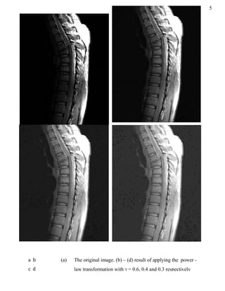
3.2.3 Power-law transformation
Power-law transformations have the basic form,
s = c*r. ^, where c and are positive constants.
The commands,
>> f = imread ('Fig3.08(a).jpg');
f = im2double (f);
[m n]=size (f);
c = 1;
gama = input('gama value = ');
for i=1:m
for j=1:n
g(i,j)=c*(f(i,j)^gama);
end
end;
imshow(f),figure, imshow(g);
With = 0.6, 0.4 and 0.3 respectively, we can get three images respectively, as shown in the
following figure,](https://image.slidesharecdn.com/digital-image-processing-using-matlab-basic-transformations-filters-operators-140529193837-phpapp01/85/Digital-image-processing-using-matlab-basic-transformations-filters-and-operators-5-320.jpg)

![7
3.2.4 Piecewise-linear transformation
Contrast stretching
The commands,
% function contrast stretching;
>> r1 = 100; s1 = 40;
r2 = 141; s2 = 216;
a = (s1/r1);
b = ((s2-s1)/ (r2-r1));
c = ((255-s2)/ (255-r2));
k = 0:r1;
y1 = a*k;
plot (k,y1); hold on;
k = r1: r2;
y2 = b*(k - r1) + a*r1;
plot (k,y2);
k = r2+1:255;
y3 = c*(k-r2) + b*(r2-r1)+a*r1;
plot (k,y3);
xlim([0 255]);
ylim([0 255]);
xlabel('input gray level, r');
ylabel('outphut gray level, s');
title('Form of transformation');
hold on; figure;
f = imread('Fig3.10(b).jpg');
[m, n] = size (f);
for i = 1:m
for j = 1:n
if((f(i,j)>=0) & (f(i,j)<=r1))
g(i,j) = a*f(i,j);
else
if((f(i,j)>r1) & (f(i,j)<=r2))
g(i,j) = ((b*(f(i,j)-r1)+(a*r1)));
else
if((f(i,j)>r2) & (f(i,j)<=255))
g(i,j) = ((c*(f(i,j)-r2)+(b*(r2-r1)+(a*r1))));
end
end
end
end
end
imshow(f), figure, imshow(g);
% function thresholding
>> f = imread('Fig3.10(b).jpg');
[m, n] = size(f);
for i = 1:m
for j = 1:n
if((f(i,j)>=0) & (f(i,j)<128))](https://image.slidesharecdn.com/digital-image-processing-using-matlab-basic-transformations-filters-operators-140529193837-phpapp01/85/Digital-image-processing-using-matlab-basic-transformations-filters-and-operators-8-320.jpg)


![14
3.6.1 Smoothing Linear Filters
The commands,
f = imread('Fig3.35(a).jpg');
w3 = 1/ (3. ^2)*ones (3);
g3 = imfilter (f, w3, 'conv', 'replicate', 'same');
w5 = 1/ (5. ^2)*ones (5);
g5 = imfilter (f, w5, 'conv', 'replicate', 'same');
w9 = 1/ (9. ^2)*ones (9);
g9 = imfilter (f, w9, 'conv', 'replicate', 'same');
w15 = 1/ (15. ^2)*ones (15);
g15 = imfilter (f, w15, 'conv', 'replicate', 'same');
w35 = 1/ (35. ^2)*ones (35);
g35 = imfilter(f, w35, 'conv', 'replicate', 'same');
imshow (g3), figure, imshow (g5), figure, imshow (g9), figure, imshow
(g15), figure, imshow (g35), figure;
h = imread ('Fig3.36(a).jpg');
h15 = imfilter (h, w15, 'conv', 'replicate', 'same');
[m, n] = size (h15);
for i = 1:m
for j = 1:n
if ((h15 (i,j)>=0) & (h15 (i,j)<128))
g (i,j) = 0;
else
g(i,j) = 255;
end
end
end
imshow(h15), figure, imshow(g);](https://image.slidesharecdn.com/digital-image-processing-using-matlab-basic-transformations-filters-operators-140529193837-phpapp01/85/Digital-image-processing-using-matlab-basic-transformations-filters-and-operators-15-320.jpg)

![17
3.7.2 The Laplacian
The Laplacian for image enhancement is as follows:
( )
{
( ) ( )
( ) ( )
( )
The commands,
% Laplacian function
f1 = imread('Fig3.40(a).jpg');
w4 = fspecial('laplacian', 0);
g1 = imfilter(f1, w4, 'replicate');
imshow(g1, [ ]), figure;
f2 = im2double(f1);
g2 = imfilter(f2, w4, 'replicate');
imshow(g2, [ ]), figure;
g3 = imsubtract(f2,g2);
imshow(g3)
Fig. 3.40 (a) Image of
the North Pole
of the moon.
(b) Laplacian
image scaled
for display
purposes. (d)
Image
enhanced by
Eq. (3.7 – 5)
a b
c d](https://image.slidesharecdn.com/digital-image-processing-using-matlab-basic-transformations-filters-operators-140529193837-phpapp01/85/Digital-image-processing-using-matlab-basic-transformations-filters-and-operators-18-320.jpg)
![18
% Laplacian simplication
f1 = imread ('Fig3.41(c).jpg');
w5 = [0 -1 0; -1 5 -1; 0 -1 0];
g1 = imfilter (f1, w5, 'replicate');
imshow (g1), figure;
w9 = [-1 -1 -1; -1 9 -1; -1 -1 -1];
g2 = imfilter (f1, w9, 'replicate');
imshow (g2);
0 -1 0
-1 5 -1
0 -1 0
-1 -1 -1
-1 9 -1
-1 -1 -1
a b c
d e
Fig. 3.37 (a) Composite Laplacian mask. (b) A second composite
mask. (c) Scanning electron microscope image. (d) and (e)
Result of filtering with the masks in (a) and (b) respectively.](https://image.slidesharecdn.com/digital-image-processing-using-matlab-basic-transformations-filters-operators-140529193837-phpapp01/85/Digital-image-processing-using-matlab-basic-transformations-filters-and-operators-19-320.jpg)
Ad
Recommended
3. INTRODUCTION TO PROTECTIVE RELAYING.pptx
3. INTRODUCTION TO PROTECTIVE RELAYING.pptxMuhd Hafizi Idris The document provides a comprehensive overview of protective relaying in power systems, detailing the functions, requirements, and types of protection schemes including unit and non-unit protections. It discusses various components of protection systems, different types of protective relays based on technology (electromechanical, solid state, and digital), and their respective advantages and disadvantages. Additionally, the document covers the ANSI standard device numbers used to identify protective devices in schematic diagrams.
Enhancement in spatial domain
Enhancement in spatial domainAshish Kumar Spatial domain image enhancement techniques operate directly on pixel values. Some common techniques include point processing using gray level transformations, mask processing using filters, and histogram processing. Histogram equalization aims to create a uniform distribution of pixel values by mapping the original histogram to a wider range. This improves contrast by distributing pixels more evenly across gray levels.
Chapter 3 image enhancement (spatial domain)
Chapter 3 image enhancement (spatial domain)asodariyabhavesh This document discusses various intensity transformation and spatial filtering techniques for digital image enhancement. It covers single pixel operations like negative image and contrast stretching. It also discusses neighborhood operations such as averaging and median filters. Finally, it discusses geometric spatial transformations like scaling, rotation and translation. The document provides details on basic intensity transformation functions including log, power law, and piecewise linear transformations. It also covers histogram processing techniques like histogram equalization, matching and local histogram processing. Spatial filtering and its mechanics are explained.
Image Restoration (Frequency Domain Filters):Basics
Image Restoration (Frequency Domain Filters):BasicsKalyan Acharjya The document discusses various frequency domain filters used in image restoration, categorizing them into types such as low-pass, high-pass, band-pass, and band-stop filters. It explains the principles of image restoration techniques aimed at recovering degraded images, utilizing Fourier transforms for processing. Additionally, it covers advanced topics like notch filters and adaptive filters, emphasizing their roles in noise removal and image enhancement.
Digital Image Processing - Image Restoration
Digital Image Processing - Image RestorationMathankumar S The document covers image restoration techniques aimed at recovering degraded images, emphasizing the use of a priori knowledge about degradation phenomena. It discusses various methods such as unconstrained and constrained restoration, inverse filtering, and interactive restoration, detailing concepts like noise models and training in artificial neural networks. Additionally, it explores different degradation models and approaches for blind image restoration.
Image processing second unit Notes
Image processing second unit NotesAAKANKSHA JAIN The document discusses advanced image processing techniques, specifically focusing on image enhancement methods divided into spatial and frequency domain methods. It explores various gray-level transformations, histogram processing techniques, and arithmetic/logic operations for enhancing image definition, specifically pointing out tools like histogram equalization and image subtraction. These techniques are applied to improve the suitability of images for specific applications, ranging from medical imaging to surveillance.
LAPLACE TRANSFORM SUITABILITY FOR IMAGE PROCESSING
LAPLACE TRANSFORM SUITABILITY FOR IMAGE PROCESSINGPriyanka Rathore Image processing techniques can involve converting images to digital form and applying transformations like the Laplace transform. The Laplace transform is useful for applications like image sharpening, edge detection, and blob detection. It involves calculating the second derivative of the image to help identify edges and other discontinuities. The zero crossings of the Laplace transform output are particularly useful for edge detection as they indicate where the slope of the image changes most rapidly. While the Laplace transform provides benefits like simpler implementation and reliable noise performance, it can also result in spaghetti-like edge effects with complex computations.
Diabetes Mellitus
Diabetes MellitusMD Abdul Haleem This document provides an overview of diabetes mellitus (DM), including the three main types (Type 1, Type 2, and gestational diabetes), signs and symptoms, complications, pathophysiology, oral manifestations, dental management considerations, emergency management, diagnosis, and treatment. DM is caused by either the pancreas not producing enough insulin or cells not responding properly to insulin, resulting in high blood sugar levels. The document compares and contrasts the characteristics of Type 1 and Type 2 DM.
Image segmentation
Image segmentation Tubur Borgoary This document summarizes techniques for image segmentation based on global thresholding and gradient-based edge detection. It discusses image segmentation, approaches like thresholding and edge detection in MATLAB. Thresholding is demonstrated on sample images to extract objects at different threshold values. Edge detection is also shown using Sobel filters. Issues like segmenting similar objects and boundary detection in the presence of noise are mentioned.
6.frequency domain image_processing
6.frequency domain image_processingNashid Alam 1. The document discusses image processing in the frequency domain, which involves transforming an image into its frequency distribution using mathematical operators called transformations like the Fourier transform.
2. The Fourier transform decomposes an image into its frequency components, which can be divided into high frequency components corresponding to edges and low frequency components corresponding to smooth regions.
3. An example computes the 2D discrete Fourier transform of a toy image using zero-padding to increase resolution, and the fftshift function is used to center the DC coefficient when visualizing the transformed image.
Spatial filtering using image processing
Spatial filtering using image processingAnuj Arora (1) Spatial filtering is defined as operations performed on pixels within a neighborhood of an image using a mask or kernel. (2) Filters can be used to blur/smooth an image by reducing noise or sharpen an image by enhancing edges. (3) Common linear filtering methods include averaging, Gaussian, and derivative filters which are implemented using various mask patterns to modify pixels in the filtered image.
Image processing
Image processingMohammed Abraruddin This document provides an overview of image processing and related concepts. It discusses:
1) What an image is, the basic steps of image processing like acquisition, analysis and output, and the two main types: analogue and digital.
2) Key aspects of digital image processing including what a digital image and pixel are, and common processing steps of pre-processing, enhancement and extraction.
3) Common image processing techniques like enhancement which adjusts images, and segmentation which partitions an image into meaningful segments.
4) Image classification which predicts categories from inputs, and the main types of supervised and unsupervised classification. It provides an example using Landsat satellite images.
Image Processing
Image Processingtijeel Homomorphic filtering is an image enhancement technique that normalizes brightness across an image and increases contrast. It involves taking the logarithm of an image to separate it into illumination and reflectance components, applying a frequency domain filter, and then taking the exponential to reconstruct an enhanced image with reduced intensity variation and highlighted details. Homomorphic filtering has applications in areas like astronomy, medicine, security, and defense.
image enhancement
image enhancementRajendra Prasad Image enhancement techniques can be divided into spatial and frequency domain methods. Spatial domain methods operate directly on pixel values using techniques like basic gray level transformations, contrast stretching and thresholding. These manipulations are used to accentuate image features, improve display quality or aid machine analysis by modifying pixel intensities within an image.
Image processing SaltPepper Noise
Image processing SaltPepper NoiseAnkush Srivastava This document discusses image noise reduction systems. It defines two main types of images - vector images defined by control points and digital images defined as 2D arrays of pixels. It describes different types of digital images like binary, grayscale, and color images. It then discusses image noise sources, types of noise like salt and pepper, Gaussian, speckle and periodic noise. Various noise filtering techniques are presented like minimum, maximum, mean, median and rank order filtering to remove salt and pepper noise.
Image enhancement
Image enhancementKuppusamy P The document discusses various image enhancement techniques aimed at improving the perception of information in images. It covers methods in both spatial and frequency domains, including point operations, contrast stretching, histogram modeling, and Fourier transforms, explaining how each enhances image features without increasing inherent information content. The text emphasizes the importance of these techniques for better input in image processing and analysis.
Digital Image Processing
Digital Image Processinglalithambiga kamaraj This document summarizes techniques for least mean square filtering and geometric transformations. It discusses minimum mean square error (Wiener) filtering, constrained least squares filtering, and geometric mean filtering for noise removal. It also covers spatial transformations, nearest neighbor gray level interpolation, and bilinear interpolation for geometric correction of distorted images. Examples are provided to demonstrate geometric distortion, nearest neighbor interpolation, and bilinear transformation.
Region filling
Region fillinghetvi naik This document describes a morphological region filling algorithm. It begins with a binary image X containing a single seed point p set to 1, while all other points are 0. The algorithm then repeatedly dilates X, takes the complement, and intersects with the boundary pixels of the object A until convergence. The final filled region is the union of A and the converged X, containing both the filled interior and original boundary. An example implementation fills holes in a binary coin image by applying this algorithm.
Fundamentals of Image Processing & Computer Vision with MATLAB
Fundamentals of Image Processing & Computer Vision with MATLABAli Ghanbarzadeh The document provides a comprehensive introduction to MATLAB including its user interface and basic functionalities such as matrix manipulations, plotting, and algorithm implementation. It covers various topics such as image processing and computer vision, explaining the use of MATLAB toolboxes for image analysis, enhancement, and segmentation techniques. Additionally, it discusses advanced topics like calculus, functions, and filtering processes in image processing, along with practical examples and code snippets.
IRJET- Color Balance and Fusion for Underwater Image Enhancement: Survey
IRJET- Color Balance and Fusion for Underwater Image Enhancement: SurveyIRJET Journal This document summarizes research on methods for enhancing underwater images. It discusses how underwater images suffer from poor visibility due to light scattering and absorption in water. Several approaches are then summarized that aim to restore and enhance degraded underwater images through techniques like color balance and fusion. Specifically, the document surveys methods that use single-image approaches without specialized hardware by fusing color-compensated and white-balanced versions of the original image. It also discusses other literature on underwater image enhancement through techniques like dehazing, wavelength compensation, and contrast adjustment.
Module 31
Module 31UllasSS1 The document discusses image restoration techniques. It introduces common image degradation models and noise models encountered in imaging. Spatial and frequency domain filtering methods are described for restoration when the degradation is additive noise. Adaptive median filtering and frequency domain filtering techniques like bandreject, bandpass and notch filters are explained for periodic noise removal. Optimal filtering methods like Wiener filtering that minimize mean square error are also covered. The document provides an overview of key concepts and methods in image restoration.
Spatial operation.ppt
Spatial operation.pptBhanubhakta Poudel This document discusses different types of spatial filters that can be applied to images, including low-pass, high-pass, average, and median filters. Spatial filters work by applying a filter mask over an image and calculating new pixel values based on the neighborhood defined by the mask. Low-pass filters preserve low frequencies and are used for smoothing and blurring to reduce noise or small details. High-pass filters preserve high frequencies and are used to highlight edges and detail. Average filters reduce irrelevant detail through normalization, while median filters are effective for reducing salt-and-pepper noise with less blurring than linear filters.
COM2304: Intensity Transformation and Spatial Filtering – II Spatial Filterin...
COM2304: Intensity Transformation and Spatial Filtering – II Spatial Filterin...Hemantha Kulathilake The document outlines the fundamentals of spatial filtering in computer graphics and image processing, detailing the generation of spatial filter masks and the application of both linear and non-linear smoothing techniques. It explains how filters can suppress high or low frequencies in images and emphasizes the importance of convolution and correlation in filtering processes. Various types of smoothing filters, including mean, geometric mean, harmonic mean, and median filters, are discussed along with their specific uses and effects on image quality.
Sharpening using frequency Domain Filter
Sharpening using frequency Domain Filterarulraj121 This document discusses frequency domain filtering for image sharpening. It begins by explaining the difference between spatial and frequency domain image enhancement techniques. It then describes the basic steps for filtering in the frequency domain, which involves taking the Fourier transform of an image, multiplying it by a filter function, and taking the inverse Fourier transform. The document discusses sharpening filters specifically, noting that high-pass filters can be used to sharpen by preserving high frequency components that represent edges. It provides examples of ideal low-pass and high-pass filters, and Butterworth and Gaussian filters. Laplacian filters are also introduced as a common sharpening filter that uses an approximation of second derivatives to detect and enhance edges.
Comparison of image segmentation
Comparison of image segmentationHaitham Ahmed The document evaluates three image segmentation algorithms: mean shift segmentation, efficient graph-based segmentation, and a hybrid approach combining the first two. It assesses their performance based on correctness, stability with respect to parameter choices, and stability across different images, using the normalized probabilistic rand index for comparison. The findings suggest that the hybrid method offers better stability and performance over a range of parameters compared to the other two algorithms.
Unit vi
Unit viswapnasalil 1. Animation involves rapidly displaying sequential images to create the illusion of motion. It can be done by hand drawing or using software to animate graphics.
2. There are two main types of animators - lead artists who draw key frames showing major changes, and assistants who draw intermediate frames between key frames through a process called tweening.
3. Techniques of animation include onion skinning to see frames flow together, motion cycling for repetitive motions, and masking to make objects move behind protected areas of the frame. Color cycling and morphing are also techniques.
Psuedo color
Psuedo colorMariashoukat1206 The document discusses pseudo color images and techniques for converting grayscale images to color. It defines pseudo color images as grayscale images mapped to color according to a lookup table or function. It describes various color schemes for this mapping, including grayscale schemes that use shades of gray and oscillating schemes that emphasize certain grayscale ranges in color. The document also discusses using piecewise linear functions and smooth non-linear functions to transform grayscale levels to color for purposes such as enhancing contrast or reducing noise in images.
Image processing Presentation
Image processing PresentationValia koonambaikulathamma college of engineering and technology The document discusses the key components of an image processing system, including image sensing, digitization, storage, and display. It covers common image sensing devices like cameras, scanners, and MRI systems. It also describes digitizers, different types of digital storage, and principal display devices. Finally, it discusses concepts like spatial and gray-level resolution, sampling and quantization, and interpolation methods used for zooming and shrinking digital images.
annotated-chap-3-gw.ppt
annotated-chap-3-gw.pptTharshninipriyaRajas This document discusses intensity transformation and spatial filtering of digital images. It begins by distinguishing between processing images in the spatial domain versus the transform domain. In the spatial domain, pixel intensities are directly modified based on an operator applied to a neighborhood of pixels. Intensity transformations modify pixel values based on an intensity transformation function. Examples of basic intensity transformations discussed include image negatives, log transformations, power-law (gamma) transformations, and piecewise-linear transformations. Histogram processing techniques like histogram equalization, matching, and analysis are also covered.
Aistats RTD
Aistats RTDYuma Murakami The document proposes an algorithm called Robust Tensor Decomposition (RTD) to recover a low-rank tensor from observations that are corrupted by block sparse errors. RTD iteratively estimates the low-rank and sparse components using hard thresholding and tensor projections. It compares RTD to existing approaches on video sequences, finding RTD yields more accurate recovery with fewer assumptions.
More Related Content
What's hot (20)
Image segmentation
Image segmentation Tubur Borgoary This document summarizes techniques for image segmentation based on global thresholding and gradient-based edge detection. It discusses image segmentation, approaches like thresholding and edge detection in MATLAB. Thresholding is demonstrated on sample images to extract objects at different threshold values. Edge detection is also shown using Sobel filters. Issues like segmenting similar objects and boundary detection in the presence of noise are mentioned.
6.frequency domain image_processing
6.frequency domain image_processingNashid Alam 1. The document discusses image processing in the frequency domain, which involves transforming an image into its frequency distribution using mathematical operators called transformations like the Fourier transform.
2. The Fourier transform decomposes an image into its frequency components, which can be divided into high frequency components corresponding to edges and low frequency components corresponding to smooth regions.
3. An example computes the 2D discrete Fourier transform of a toy image using zero-padding to increase resolution, and the fftshift function is used to center the DC coefficient when visualizing the transformed image.
Spatial filtering using image processing
Spatial filtering using image processingAnuj Arora (1) Spatial filtering is defined as operations performed on pixels within a neighborhood of an image using a mask or kernel. (2) Filters can be used to blur/smooth an image by reducing noise or sharpen an image by enhancing edges. (3) Common linear filtering methods include averaging, Gaussian, and derivative filters which are implemented using various mask patterns to modify pixels in the filtered image.
Image processing
Image processingMohammed Abraruddin This document provides an overview of image processing and related concepts. It discusses:
1) What an image is, the basic steps of image processing like acquisition, analysis and output, and the two main types: analogue and digital.
2) Key aspects of digital image processing including what a digital image and pixel are, and common processing steps of pre-processing, enhancement and extraction.
3) Common image processing techniques like enhancement which adjusts images, and segmentation which partitions an image into meaningful segments.
4) Image classification which predicts categories from inputs, and the main types of supervised and unsupervised classification. It provides an example using Landsat satellite images.
Image Processing
Image Processingtijeel Homomorphic filtering is an image enhancement technique that normalizes brightness across an image and increases contrast. It involves taking the logarithm of an image to separate it into illumination and reflectance components, applying a frequency domain filter, and then taking the exponential to reconstruct an enhanced image with reduced intensity variation and highlighted details. Homomorphic filtering has applications in areas like astronomy, medicine, security, and defense.
image enhancement
image enhancementRajendra Prasad Image enhancement techniques can be divided into spatial and frequency domain methods. Spatial domain methods operate directly on pixel values using techniques like basic gray level transformations, contrast stretching and thresholding. These manipulations are used to accentuate image features, improve display quality or aid machine analysis by modifying pixel intensities within an image.
Image processing SaltPepper Noise
Image processing SaltPepper NoiseAnkush Srivastava This document discusses image noise reduction systems. It defines two main types of images - vector images defined by control points and digital images defined as 2D arrays of pixels. It describes different types of digital images like binary, grayscale, and color images. It then discusses image noise sources, types of noise like salt and pepper, Gaussian, speckle and periodic noise. Various noise filtering techniques are presented like minimum, maximum, mean, median and rank order filtering to remove salt and pepper noise.
Image enhancement
Image enhancementKuppusamy P The document discusses various image enhancement techniques aimed at improving the perception of information in images. It covers methods in both spatial and frequency domains, including point operations, contrast stretching, histogram modeling, and Fourier transforms, explaining how each enhances image features without increasing inherent information content. The text emphasizes the importance of these techniques for better input in image processing and analysis.
Digital Image Processing
Digital Image Processinglalithambiga kamaraj This document summarizes techniques for least mean square filtering and geometric transformations. It discusses minimum mean square error (Wiener) filtering, constrained least squares filtering, and geometric mean filtering for noise removal. It also covers spatial transformations, nearest neighbor gray level interpolation, and bilinear interpolation for geometric correction of distorted images. Examples are provided to demonstrate geometric distortion, nearest neighbor interpolation, and bilinear transformation.
Region filling
Region fillinghetvi naik This document describes a morphological region filling algorithm. It begins with a binary image X containing a single seed point p set to 1, while all other points are 0. The algorithm then repeatedly dilates X, takes the complement, and intersects with the boundary pixels of the object A until convergence. The final filled region is the union of A and the converged X, containing both the filled interior and original boundary. An example implementation fills holes in a binary coin image by applying this algorithm.
Fundamentals of Image Processing & Computer Vision with MATLAB
Fundamentals of Image Processing & Computer Vision with MATLABAli Ghanbarzadeh The document provides a comprehensive introduction to MATLAB including its user interface and basic functionalities such as matrix manipulations, plotting, and algorithm implementation. It covers various topics such as image processing and computer vision, explaining the use of MATLAB toolboxes for image analysis, enhancement, and segmentation techniques. Additionally, it discusses advanced topics like calculus, functions, and filtering processes in image processing, along with practical examples and code snippets.
IRJET- Color Balance and Fusion for Underwater Image Enhancement: Survey
IRJET- Color Balance and Fusion for Underwater Image Enhancement: SurveyIRJET Journal This document summarizes research on methods for enhancing underwater images. It discusses how underwater images suffer from poor visibility due to light scattering and absorption in water. Several approaches are then summarized that aim to restore and enhance degraded underwater images through techniques like color balance and fusion. Specifically, the document surveys methods that use single-image approaches without specialized hardware by fusing color-compensated and white-balanced versions of the original image. It also discusses other literature on underwater image enhancement through techniques like dehazing, wavelength compensation, and contrast adjustment.
Module 31
Module 31UllasSS1 The document discusses image restoration techniques. It introduces common image degradation models and noise models encountered in imaging. Spatial and frequency domain filtering methods are described for restoration when the degradation is additive noise. Adaptive median filtering and frequency domain filtering techniques like bandreject, bandpass and notch filters are explained for periodic noise removal. Optimal filtering methods like Wiener filtering that minimize mean square error are also covered. The document provides an overview of key concepts and methods in image restoration.
Spatial operation.ppt
Spatial operation.pptBhanubhakta Poudel This document discusses different types of spatial filters that can be applied to images, including low-pass, high-pass, average, and median filters. Spatial filters work by applying a filter mask over an image and calculating new pixel values based on the neighborhood defined by the mask. Low-pass filters preserve low frequencies and are used for smoothing and blurring to reduce noise or small details. High-pass filters preserve high frequencies and are used to highlight edges and detail. Average filters reduce irrelevant detail through normalization, while median filters are effective for reducing salt-and-pepper noise with less blurring than linear filters.
COM2304: Intensity Transformation and Spatial Filtering – II Spatial Filterin...
COM2304: Intensity Transformation and Spatial Filtering – II Spatial Filterin...Hemantha Kulathilake The document outlines the fundamentals of spatial filtering in computer graphics and image processing, detailing the generation of spatial filter masks and the application of both linear and non-linear smoothing techniques. It explains how filters can suppress high or low frequencies in images and emphasizes the importance of convolution and correlation in filtering processes. Various types of smoothing filters, including mean, geometric mean, harmonic mean, and median filters, are discussed along with their specific uses and effects on image quality.
Sharpening using frequency Domain Filter
Sharpening using frequency Domain Filterarulraj121 This document discusses frequency domain filtering for image sharpening. It begins by explaining the difference between spatial and frequency domain image enhancement techniques. It then describes the basic steps for filtering in the frequency domain, which involves taking the Fourier transform of an image, multiplying it by a filter function, and taking the inverse Fourier transform. The document discusses sharpening filters specifically, noting that high-pass filters can be used to sharpen by preserving high frequency components that represent edges. It provides examples of ideal low-pass and high-pass filters, and Butterworth and Gaussian filters. Laplacian filters are also introduced as a common sharpening filter that uses an approximation of second derivatives to detect and enhance edges.
Comparison of image segmentation
Comparison of image segmentationHaitham Ahmed The document evaluates three image segmentation algorithms: mean shift segmentation, efficient graph-based segmentation, and a hybrid approach combining the first two. It assesses their performance based on correctness, stability with respect to parameter choices, and stability across different images, using the normalized probabilistic rand index for comparison. The findings suggest that the hybrid method offers better stability and performance over a range of parameters compared to the other two algorithms.
Unit vi
Unit viswapnasalil 1. Animation involves rapidly displaying sequential images to create the illusion of motion. It can be done by hand drawing or using software to animate graphics.
2. There are two main types of animators - lead artists who draw key frames showing major changes, and assistants who draw intermediate frames between key frames through a process called tweening.
3. Techniques of animation include onion skinning to see frames flow together, motion cycling for repetitive motions, and masking to make objects move behind protected areas of the frame. Color cycling and morphing are also techniques.
Psuedo color
Psuedo colorMariashoukat1206 The document discusses pseudo color images and techniques for converting grayscale images to color. It defines pseudo color images as grayscale images mapped to color according to a lookup table or function. It describes various color schemes for this mapping, including grayscale schemes that use shades of gray and oscillating schemes that emphasize certain grayscale ranges in color. The document also discusses using piecewise linear functions and smooth non-linear functions to transform grayscale levels to color for purposes such as enhancing contrast or reducing noise in images.
Image processing Presentation
Image processing PresentationValia koonambaikulathamma college of engineering and technology The document discusses the key components of an image processing system, including image sensing, digitization, storage, and display. It covers common image sensing devices like cameras, scanners, and MRI systems. It also describes digitizers, different types of digital storage, and principal display devices. Finally, it discusses concepts like spatial and gray-level resolution, sampling and quantization, and interpolation methods used for zooming and shrinking digital images.
COM2304: Intensity Transformation and Spatial Filtering – II Spatial Filterin...
COM2304: Intensity Transformation and Spatial Filtering – II Spatial Filterin...Hemantha Kulathilake
Similar to Digital image processing using matlab: basic transformations, filters and operators (20)
annotated-chap-3-gw.ppt
annotated-chap-3-gw.pptTharshninipriyaRajas This document discusses intensity transformation and spatial filtering of digital images. It begins by distinguishing between processing images in the spatial domain versus the transform domain. In the spatial domain, pixel intensities are directly modified based on an operator applied to a neighborhood of pixels. Intensity transformations modify pixel values based on an intensity transformation function. Examples of basic intensity transformations discussed include image negatives, log transformations, power-law (gamma) transformations, and piecewise-linear transformations. Histogram processing techniques like histogram equalization, matching, and analysis are also covered.
Aistats RTD
Aistats RTDYuma Murakami The document proposes an algorithm called Robust Tensor Decomposition (RTD) to recover a low-rank tensor from observations that are corrupted by block sparse errors. RTD iteratively estimates the low-rank and sparse components using hard thresholding and tensor projections. It compares RTD to existing approaches on video sequences, finding RTD yields more accurate recovery with fewer assumptions.
Existing method used for analysis of images
Existing method used for analysis of imagesssuser1ecccc Chapter 6 presents experimental results on watermarking methods using images collected from various sources, highlighting the psnr and mse values for embedded and extracted watermarked images. The proposed method successfully embeds secret images into video frames, with performance metrics indicating the effectiveness of the watermarking technique. Additionally, the document discusses scene changes during video reconstruction, correlating them with different watermark images.
matlab.docx
matlab.docxAraniNavaratnarajah2 This MATLAB code applies the Roberts edge detection filter to an input image. It first reads in the image and converts it to grayscale. It then initializes an output matrix to store the filtered image. Next, it defines the Roberts filter masks and loops through the image, calculating the gradient approximations in the x and y directions using the masks. It calculates the magnitude of the gradient vector and stores it in the output matrix. Finally, it displays the original and filtered images, with the filtered image highlighting edges detected by the Roberts filter.
G Intensity transformation and spatial filtering(1).ppt
G Intensity transformation and spatial filtering(1).pptdeekshithadasari26 The document covers intensity transformation and spatial filtering in image processing, distinguishing between spatial and transform domains. It discusses various techniques such as logarithmic and gamma transformations, contrast stretching, histogram equalization, and histogram matching. The document also includes examples and procedures for applying these transformations to enhance image quality.
Lect 03 - first portion
Lect 03 - first portionMoe Moe Myint The document discusses various image enhancement techniques in the spatial domain. It covers basic gray level transformations like negatives, log transformations, and power law transformations. It also discusses histogram processing and enhancement using arithmetic operations. Furthermore, it explains smoothing and sharpening spatial filters, and how to combine different spatial enhancement methods. The document provides examples and background on these fundamental image enhancement concepts.
Histogram processing
Histogram processingVisvesvaraya National Institute of Technology, Nagpur, Maharashtra, India Setting the lower order bit plane to zero would have the effect of reducing the number of distinct gray levels by half. This would cause the histogram to become more peaked, with more pixels concentrated in fewer bins.
Ch 3. Image Enhancement in the Spatial Domain_okay.ppt
Ch 3. Image Enhancement in the Spatial Domain_okay.pptnurulrahat02 The document discusses image enhancement techniques in the spatial domain, detailing methods such as gray-level transformations, histogram processing, and filtering approaches. It covers various enhancement strategies including contrast stretching, histogram equalization, smoothing and sharpening filters, and arithmetic operations. Additionally, it explains the mathematical foundations underlying these techniques and their applications in image processing.
Notes on image processing
Notes on image processingMohammed Kamel Edge detection is used to identify points in a digital image where the image brightness changes sharply. The key steps are smoothing to reduce noise, enhancing edges through differentiation, thresholding to determine important edges, and localization to find edge positions. Common methods include using the first derivative to find gradients and zero-crossings of the second derivative. Operators like Prewitt and Sobel approximate derivatives with small pixel masks. Edge detection is useful for computer vision tasks by extracting important image features.
DIP_Manual.pdf
DIP_Manual.pdfNetraBahadurKatuwal This document outlines 13 experiments for a digital image processing lab manual, including: 1) displaying color/grayscale images and their negatives, 2) analyzing pixel relationships, 3) applying image transformations, 4) enhancing low contrast images using histogram equalization, 5) examining bit planes, 6) computing FFTs, 7) analyzing image statistics, 8) applying smoothing/median filters, 9) detecting edges using gradient filters, 10) compressing images, 11) restoring images, 12) enhancing using intensity slicing, and 13) detecting edges with Canny edge detection. The document was prepared by Abhishek Appaji.
1.funtions (1)
1.funtions (1)josnihmurni2907 The document contains 13 math problems involving functions. The problems cover topics such as:
- Finding the image and object of elements under a given function
- Finding inverse functions
- Determining the type of relation between sets
- Evaluating composite functions
- Solving for unknown constants in function definitions
- Finding the value of x when a composite function equals a given value
The document provides the problems and blank spaces for the answers. The answers section gives the solutions to each of the 13 problems.
Digital Image processing is the class of methods that deal with manipulating ...
Digital Image processing is the class of methods that deal with manipulating ...kusumrao5 The document outlines the image restoration process, detailing various models of image degradation and restoration techniques, including filtering methods like inverse and Wiener filtering. It emphasizes the objective of restoring degraded images to their original form while addressing noise that may affect image quality. Additionally, it covers the estimation of degradation functions through image observation, experimentation, and modeling, alongside discussions of geometric transformations in image processing.
Lect02.ppt
Lect02.pptRaniaAzad This document discusses intensity transformation and spatial filtering in digital image processing. It covers spatial domain vs transform domain processing, and various spatial domain intensity transformation functions including image negatives, log transformations, power-law (gamma) transformations, and piecewise-linear transformations. Histogram processing techniques like histogram equalization, histogram matching, and local histogram processing are also introduced. Examples are provided to illustrate different intensity transformations and histogram matching.
ch-2.2 histogram image processing .pptx
ch-2.2 histogram image processing .pptxsatyanarayana242612 The document discusses histogram processing in digital image enhancement, detailing how histograms represent the frequency of gray levels in an image. It explores various methods for histogram plotting and their advantages, particularly focusing on histogram stretching and equalization techniques to improve image contrast. Additionally, it provides examples and a mathematical framework for transforming image histograms towards a desired flat distribution.
Funções 1
Funções 1KalculosOnline The document contains 15 multiple choice questions about functions. The questions cover topics such as exponential decay functions, quadratic functions, maximum and minimum values of functions, and function definitions and properties.
Introduction to image contrast and enhancement method
Introduction to image contrast and enhancement methodAbhishekvb This document discusses various methods for contrast enhancement of digital images. It defines contrast and describes how contrast is important for distinguishing objects from backgrounds. Two main categories of contrast enhancement methods are described: spatial domain methods, which operate directly on pixel values; and frequency domain methods, which modify the Fourier transform of an image. Specific spatial techniques covered include logarithmic transformation, power law transformation, gamma correction, and histogram equalization. Contrast stretching is also discussed. Examples of code implementations and results are provided. Contrast enhancement has applications in medical imaging, surveillance, and other fields where improving image interpretability is important.
Hand book of Howard Anton calculus exercises 8th edition
Hand book of Howard Anton calculus exercises 8th editionPriSim The document contains the table of contents for a calculus textbook. It lists 17 chapters covering topics such as functions, limits, derivatives, integrals, vector calculus, and applications of calculus. It also includes 6 appendices reviewing concepts in real numbers, trigonometry, coordinate planes, and polynomial equations.
Computer vision 3 4
Computer vision 3 4sachinmore76 This document discusses image transforms and processing techniques in computer vision. It introduces important 2D linear transforms like the discrete cosine transform. It explains how transforms allow recovering the original image using the inverse transform. Examples are provided on image denoising using DCT. Probabilistic methods for analyzing images like calculating mean, variance and moments are also described. The document contrasts processing images in the spatial vs transform domains. Several basic intensity transformation functions are illustrated including negatives, log transforms, and piecewise linear transformations. Histogram processing techniques like equalization and matching are explained in detail with examples.
Image Processing Homework 1
Image Processing Homework 1Joshua Smith This document summarizes a student's work on an image processing homework assignment. The student was tasked with using histogram equalization techniques to reveal a hidden message in an provided image. The student wrote MATLAB code to perform histogram equalization on the full image and sections of the image. Equalizing the entire image did not clearly show the message, but equalizing a section revealed the word "Congratulation!" more clearly. Further dividing and equalizing the section produced the best results, mostly revealing the hidden message. The student concluded more practice with histogram equalization and combining it with other transformations could improve the results.
Ad
Recently uploaded (20)
Great Governors' Send-Off Quiz 2025 Prelims IIT KGP
Great Governors' Send-Off Quiz 2025 Prelims IIT KGPIIT Kharagpur Quiz Club Prelims of the Great Governors' Send-Off Quiz 2025 hosted by the outgoing governors.
QMs: Aarushi, Aatir, Aditya, Arnav
List View Components in Odoo 18 - Odoo Slides
List View Components in Odoo 18 - Odoo SlidesCeline George In Odoo, there are many types of views possible like List view, Kanban view, Calendar view, Pivot view, Search view, etc.
The major change that introduced in the Odoo 18 technical part in creating views is the tag <tree> got replaced with the <list> for creating list views.
OBSESSIVE COMPULSIVE DISORDER.pptx IN 5TH SEMESTER B.SC NURSING, 2ND YEAR GNM...
OBSESSIVE COMPULSIVE DISORDER.pptx IN 5TH SEMESTER B.SC NURSING, 2ND YEAR GNM...parmarjuli1412 OBSESSIVE COMPULSIVE DISORDER INCLUDED TOPICS ARE INTRODUCTION, DEFINITION OF OBSESSION, DEFINITION OF COMPULSION, MEANING OF OBSESSION AND COMPULSION, DEFINITION OF OBSESSIVE COMPULSIVE DISORDER, EPIDERMIOLOGY OF OCD, ETIOLOGICAL FACTORS OF OCD, CLINICAL SIGN AND SYMPTOMS OF OBSESSION AND COMPULSION, MANAGEMENT INCLUDED PHARMACOTHERAPY(ANTIDEPRESSANT DRUG+ANXIOLYTIC DRUGS), PSYCHOTHERAPY, NURSING MANAGEMENT(ASSESSMENT+DIAGNOSIS+NURSING INTERVENTION+EVALUATION))
M&A5 Q1 1 differentiate evolving early Philippine conventional and contempora...
M&A5 Q1 1 differentiate evolving early Philippine conventional and contempora...ErlizaRosete MAPEH 6 QI WEEK I
SCHIZOPHRENIA OTHER PSYCHOTIC DISORDER LIKE Persistent delusion/Capgras syndr...
SCHIZOPHRENIA OTHER PSYCHOTIC DISORDER LIKE Persistent delusion/Capgras syndr...parmarjuli1412 SCHIZOPHRENIA INCLUDED TOPIC IS INTRODUCTION, DEFINITION OF GENERAL TERM IN PSYCHIATRIC, THEN DIFINITION OF SCHIZOPHRENIA, EPIDERMIOLOGY, ETIOLOGICAL FACTORS, CLINICAL FEATURE(SIGN AND SYMPTOMS OF SCHIZOPHRENIA), CLINICAL TYPES OF SCHIZOPHRENIA, DIAGNOSIS, INVESTIGATION, TREATMENT MODALITIES(PHARMACOLOGICAL MANAGEMENT, PSYCHOTHERAPY, ECT, PSYCHO-SOCIO-REHABILITATION), NURSING MANAGEMENT(ASSESSMENT,DIAGNOSIS,NURSING INTERVENTION,AND EVALUATION), OTHER PSYCHOTIC DISORDER LIKE Persistent delusion/Capgras syndrome(The Delusion of Doubles)/Acute and Transient Psychotic Disorders/Induced Delusional Disorders/Schizoaffective Disorder /CAPGRAS SYNDROME(DELUSION OF DOUBLE), GERIATRIC CONSIDERATION, FOLLOW UP, HOMECARE AND REHABILITATION OF THE PATIENT,
LAZY SUNDAY QUIZ "A GENERAL QUIZ" JUNE 2025 SMC QUIZ CLUB, SILCHAR MEDICAL CO...
LAZY SUNDAY QUIZ "A GENERAL QUIZ" JUNE 2025 SMC QUIZ CLUB, SILCHAR MEDICAL CO...Ultimatewinner0342 🧠 Lazy Sunday Quiz | General Knowledge Trivia by SMC Quiz Club – Silchar Medical College
Presenting the Lazy Sunday Quiz, a fun and thought-provoking general knowledge quiz created by the SMC Quiz Club of Silchar Medical College & Hospital (SMCH). This quiz is designed for casual learners, quiz enthusiasts, and competitive teams looking for a diverse, engaging set of questions with clean visuals and smart clues.
🎯 What is the Lazy Sunday Quiz?
The Lazy Sunday Quiz is a light-hearted yet intellectually rewarding quiz session held under the SMC Quiz Club banner. It’s a general quiz covering a mix of current affairs, pop culture, history, India, sports, medicine, science, and more.
Whether you’re hosting a quiz event, preparing a session for students, or just looking for quality trivia to enjoy with friends, this PowerPoint deck is perfect for you.
📋 Quiz Format & Structure
Total Questions: ~50
Types: MCQs, one-liners, image-based, visual connects, lateral thinking
Rounds: Warm-up, Main Quiz, Visual Round, Connects (optional bonus)
Design: Simple, clear slides with answer explanations included
Tools Needed: Just a projector or screen – ready to use!
🧠 Who Is It For?
College quiz clubs
School or medical students
Teachers or faculty for classroom engagement
Event organizers needing quiz content
Quizzers preparing for competitions
Freelancers building quiz portfolios
💡 Why Use This Quiz?
Ready-made, high-quality content
Curated with lateral thinking and storytelling in mind
Covers both academic and pop culture topics
Designed by a quizzer with real event experience
Usable in inter-college fests, informal quizzes, or Sunday brain workouts
📚 About the Creators
This quiz has been created by Rana Mayank Pratap, an MBBS student and quizmaster at SMC Quiz Club, Silchar Medical College. The club aims to promote a culture of curiosity and smart thinking through weekly and monthly quiz events.
🔍 SEO Tags:
quiz, general knowledge quiz, trivia quiz, SlideShare quiz, college quiz, fun quiz, medical college quiz, India quiz, pop culture quiz, visual quiz, MCQ quiz, connect quiz, science quiz, current affairs quiz, SMC Quiz Club, Silchar Medical College
📣 Reuse & Credit
You’re free to use or adapt this quiz for your own events or sessions with credit to:
SMC Quiz Club – Silchar Medical College & Hospital
Curated by: Rana Mayank Pratap
Gladiolous Cultivation practices by AKL.pdf
Gladiolous Cultivation practices by AKL.pdfkushallamichhame This includes the overall cultivation practices of Rose prepared by:
Kushal Lamichhane (AKL)
Instructor
Shree Gandhi Adarsha Secondary School
Kageshowri Manohara-09, Kathmandu, Nepal
How to Manage Different Customer Addresses in Odoo 18 Accounting
How to Manage Different Customer Addresses in Odoo 18 AccountingCeline George A business often have customers with multiple locations such as office, warehouse, home addresses and this feature allows us to associate with different addresses with each customer streamlining the process of creating sales order invoices and delivery orders.
Pests of Maize: An comprehensive overview.pptx
Pests of Maize: An comprehensive overview.pptxArshad Shaikh Maize is susceptible to various pests that can significantly impact yields. Key pests include the fall armyworm, stem borers, cob earworms, shoot fly. These pests can cause extensive damage, from leaf feeding and stalk tunneling to grain destruction. Effective management strategies, such as integrated pest management (IPM), resistant varieties, biological control, and judicious use of chemicals, are essential to mitigate losses and ensure sustainable maize production.
ECONOMICS, DISASTER MANAGEMENT, ROAD SAFETY - STUDY MATERIAL [10TH]
ECONOMICS, DISASTER MANAGEMENT, ROAD SAFETY - STUDY MATERIAL [10TH]SHERAZ AHMAD LONE This study material for Class 10th covers the core subjects of Economics, Disaster Management, and Road Safety Education, developed strictly in line with the JKBOSE textbook. It presents the content in a simplified, structured, and student-friendly format, ensuring clarity in concepts. The material includes reframed explanations, flowcharts, infographics, and key point summaries to support better understanding and retention. Designed for classroom teaching and exam preparation, it aims to enhance comprehension, critical thinking, and practical awareness among students.
2025 June Year 9 Presentation: Subject selection.pptx
2025 June Year 9 Presentation: Subject selection.pptxmansk2 2025 June Year 9 Presentation: Subject selection
VCE Literature Section A Exam Response Guide
VCE Literature Section A Exam Response Guidejpinnuck This practical guide shows students of Unit 3&4 VCE Literature how to write responses to Section A of the exam. Including a range of examples writing about different types of texts, this guide:
*Breaks down and explains what Q1 and Q2 tasks involve and expect
*Breaks down example responses for each question
*Explains and scaffolds students to write responses for each question
*Includes a comprehensive range of sentence starters and vocabulary for responding to each question
*Includes critical theory vocabulary lists to support Q2 responses
Tanja Vujicic - PISA for Schools contact Info
Tanja Vujicic - PISA for Schools contact InfoEduSkills OECD Tanja Vujicic, Senior Analyst and PISA for School’s Project Manager at the OECD spoke at the OECD webinar 'Turning insights into impact: What do early case studies reveal about the power of PISA for Schools?' on 20 June 2025
PISA for Schools is an OECD assessment that evaluates 15-year-old performance on reading, mathematics, and science. It also gathers insights into students’ learning environment, engagement and well-being, offering schools valuable data that help them benchmark performance internationally and improve education outcomes. A central ambition, and ongoing challenge, has been translating these insights into meaningful actions that drives lasting school improvement.
Q1_ENGLISH_PPT_WEEK 1 power point grade 3 Quarter 1 week 1
Q1_ENGLISH_PPT_WEEK 1 power point grade 3 Quarter 1 week 1jutaydeonne Grade 3 Quarter 1 Week 1 English part 2
Paper 107 | From Watchdog to Lapdog: Ishiguro’s Fiction and the Rise of “Godi...
Paper 107 | From Watchdog to Lapdog: Ishiguro’s Fiction and the Rise of “Godi...Rajdeep Bavaliya Dive into a captivating analysis where Kazuo Ishiguro’s nuanced fiction meets the stark realities of post‑2014 Indian journalism. Uncover how “Godi Media” turned from watchdog to lapdog, echoing the moral compromises of Ishiguro’s protagonists. We’ll draw parallels between restrained narrative silences and sensationalist headlines—are our media heroes or traitors? Don’t forget to follow for more deep dives!
M.A. Sem - 2 | Presentation
Presentation Season - 2
Paper - 107: The Twentieth Century Literature: From World War II to the End of the Century
Submitted Date: April 4, 2025
Paper Name: The Twentieth Century Literature: From World War II to the End of the Century
Topic: From Watchdog to Lapdog: Ishiguro’s Fiction and the Rise of “Godi Media” in Post-2014 Indian Journalism
[Please copy the link and paste it into any web browser to access the content.]
Video Link: https://youtu.be/kIEqwzhHJ54
For a more in-depth discussion of this presentation, please visit the full blog post at the following link: https://rajdeepbavaliya2.blogspot.com/2025/04/from-watchdog-to-lapdog-ishiguro-s-fiction-and-the-rise-of-godi-media-in-post-2014-indian-journalism.html
Please visit this blog to explore additional presentations from this season:
Hashtags:
#GodiMedia #Ishiguro #MediaEthics #WatchdogVsLapdog #IndianJournalism #PressFreedom #LiteraryCritique #AnArtistOfTheFloatingWorld #MediaCapture #KazuoIshiguro
Keyword Tags:
Godi Media, Ishiguro fiction, post-2014 Indian journalism, media capture, Kazuo Ishiguro analysis, watchdog to lapdog, press freedom India, media ethics, literature and media, An Artist of the Floating World
Photo chemistry Power Point Presentation
Photo chemistry Power Point Presentationmprpgcwa2024 Photochemistry is the branch of chemistry that deals with the study of chemical reactions and processes initiated by light.
Photochemistry involves the interaction of light with molecules, leading to electronic excitation. Energy from light is transferred to molecules, initiating chemical reactions.
Photochemistry is used in solar cells to convert light into electrical energy.
It is used Light-driven chemical reactions for environmental remediation and synthesis. Photocatalysis helps in pollution abatement and environmental cleanup. Photodynamic therapy offers a targeted approach to treating diseases It is used in Light-activated treatment for cancer and other diseases.
Photochemistry is used to synthesize complex organic molecules.
Photochemistry contributes to the development of sustainable energy solutions.
Code Profiling in Odoo 18 - Odoo 18 Slides
Code Profiling in Odoo 18 - Odoo 18 SlidesCeline George Profiling in Odoo identifies slow code and resource-heavy processes, ensuring better system performance. Odoo code profiling detects bottlenecks in custom modules, making it easier to improve speed and scalability.
Vitamin and Nutritional Deficiencies.pptx
Vitamin and Nutritional Deficiencies.pptxVishal Chanalia Vitamin and nutritional deficiency occurs when the body does not receive enough essential nutrients, such as vitamins and minerals, needed for proper functioning. This can lead to various health problems, including weakened immunity, stunted growth, fatigue, poor wound healing, cognitive issues, and increased susceptibility to infections and diseases. Long-term deficiencies can cause serious and sometimes irreversible health complications.
Ad
Digital image processing using matlab: basic transformations, filters and operators
- 1. NATIONAL CHENG KUNG UNIVERSITY Inst. of Manufacturing Information & Systems DIGITAL IMAGE PROCESSING AND SOFTWARE IMPLEMENTATION HOMEWORK 1 Professor name: Chen, Shang-Liang Student name: Nguyen Van Thanh Student ID: P96007019 Class: P9-009 Image Processing and Software Implementation Time: [4] 2 4
- 2. 1 Table of Contents PROBLEM................................................................................................................................................................. 2 SOLUTION................................................................................................................................................................ 3 3.2.1 Negative transformation ............................................................................................................................ 3 3.2.2 Log transformation..................................................................................................................................... 3 3.2.3 Power-law transformation ......................................................................................................................... 4 3.2.4 Piecewise-linear transformation ................................................................................................................ 7 3.3.1 Histogram equalization.............................................................................................................................10 3.4.2 Subtraction ...............................................................................................................................................12 3.6.1 Smoothing Linear Filters...........................................................................................................................14 3.6.2 Order-Statistics Filters..............................................................................................................................16 3.7.2 The Laplacian............................................................................................................................................17 3.7.3 The Gradient.............................................................................................................................................19
- 3. 2 PROBLEM 影像處理與軟體實現[HW1] 課程碼:P953300 授課教授:陳響亮 教授 助教:陳怡瑄 日期:2011/03/10 題目:請以C# 撰寫一程式,可讀入一影像檔,並可執行以下之影像 空間強化功能。 a. 每一程式需設計一適當之人機操作介面。 b. 每一功能請以不同方法分開撰寫,各項參數需讓使用者自行輸入。 c. 以C# 撰寫時,可直接呼叫Matlab 現有函式,但呼叫多寡,將列為評分考量。 (呼叫越少,分數越高) 一、 基本灰階轉換 1. 影像負片轉換 2. Log轉換 3. 乘冪律轉換 4. 逐段線性函數轉換 二、 直方圖處理 1. 直方圖等化處理 2. 直方圖匹配處理 三、 使用算術/邏輯運算做增強 1. 影像相減增強 2. 影像平均增強 四、 平滑空間濾波器 1. 平滑線性濾波器 2. 排序統計濾波器 五、 銳化空間濾波器 1. 拉普拉斯銳化空間濾波器 2. 梯度銳化空間濾波器
- 4. 3 SOLUTION Using Matlab for solving the problem 3.2.1 Negative transformation Given an image (input image) with gray level in the interval [0, L-1], the negative of that image is obtained by using the expression: s = (L – 1) – r, Where r is the gray level of the input image, and s is the gray level of the output. In Matlab, we use the commands, >> f=imread('Fig3.04(a).jpg'); g = imcomplement(f); imshow(f), figure, imshow(g) In/output image Out/in image 3.2.2 Log transformation The Logarithm transformations are implemented using the expression: s = c*log (1+r). In this case, c = 1. The commands, >> f=imread('Fig3.05(a).jpg'); g=im2uint8 (mat2gray (log (1+double (f)))); imshow(f), figure, imshow(g)
- 5. 4 In/output image Out/in image 3.2.3 Power-law transformation Power-law transformations have the basic form, s = c*r. ^, where c and are positive constants. The commands, >> f = imread ('Fig3.08(a).jpg'); f = im2double (f); [m n]=size (f); c = 1; gama = input('gama value = '); for i=1:m for j=1:n g(i,j)=c*(f(i,j)^gama); end end; imshow(f),figure, imshow(g); With = 0.6, 0.4 and 0.3 respectively, we can get three images respectively, as shown in the following figure,
- 6. 5 a b c d (a) The original image. (b) – (d) result of applying the power - law transformation with = 0.6, 0.4 and 0.3 respectively
- 7. 6 a b c d (a) The original image. (b) – (d) result of applying the power - law transformation with = 3, 4 and 5 respectively
- 8. 7 3.2.4 Piecewise-linear transformation Contrast stretching The commands, % function contrast stretching; >> r1 = 100; s1 = 40; r2 = 141; s2 = 216; a = (s1/r1); b = ((s2-s1)/ (r2-r1)); c = ((255-s2)/ (255-r2)); k = 0:r1; y1 = a*k; plot (k,y1); hold on; k = r1: r2; y2 = b*(k - r1) + a*r1; plot (k,y2); k = r2+1:255; y3 = c*(k-r2) + b*(r2-r1)+a*r1; plot (k,y3); xlim([0 255]); ylim([0 255]); xlabel('input gray level, r'); ylabel('outphut gray level, s'); title('Form of transformation'); hold on; figure; f = imread('Fig3.10(b).jpg'); [m, n] = size (f); for i = 1:m for j = 1:n if((f(i,j)>=0) & (f(i,j)<=r1)) g(i,j) = a*f(i,j); else if((f(i,j)>r1) & (f(i,j)<=r2)) g(i,j) = ((b*(f(i,j)-r1)+(a*r1))); else if((f(i,j)>r2) & (f(i,j)<=255)) g(i,j) = ((c*(f(i,j)-r2)+(b*(r2-r1)+(a*r1)))); end end end end end imshow(f), figure, imshow(g); % function thresholding >> f = imread('Fig3.10(b).jpg'); [m, n] = size(f); for i = 1:m for j = 1:n if((f(i,j)>=0) & (f(i,j)<128))
- 9. 8 g(i,j) = 0; else g(i,j) = 255; end end end imshow(f), figure, imshow(g); (a) Form of contrast stretching transformation function. (b) A low-contrast image. (c) Result of contrast stretching. (d) Result of thresholding a b c d
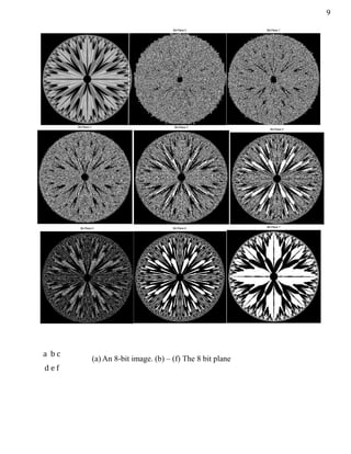
- 10. 9 (a) An 8-bit image. (b) – (f) The 8 bit plane a b c d e f
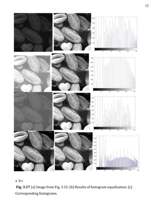
- 11. 10 3.3.1 Histogram equalization The transformation function of histogram equalization is ( ) ∑ ( ) ∑ k = 0, 1, …, L – 1. % Histogram; f1 = imread('Fig3.15(a)1top.jpg'); f2 = imread('Fig3.15(a)2.jpg'); f3 = imread('Fig3.15(a)3.jpg'); f4 = imread('Fig3.15(a)4.jpg'); f = input('image: '); imhist(f), figure; g = histeq(f, 256); imshow(g), figure, imhist(g); a b c Fig. 3.17 Transformation functions (1) through (4) were obtained from the images in Fig. 3.17 (a), using histogram equalization
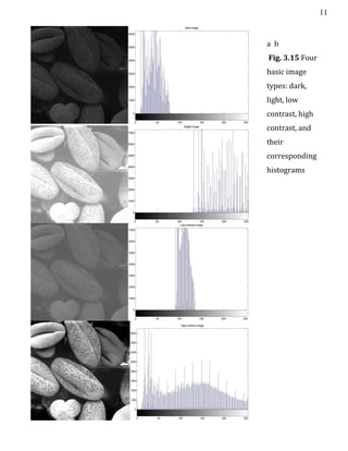
- 12. 11 a b Fig. 3.15 Four basic image types: dark, light, low contrast, high contrast, and their corresponding histograms
- 13. 12 a b c Fig. 3.17 (a) Image from Fig. 3.15. (b) Results of histogram equalization. (c) Corresponding histograms.
- 14. 13 3.4.2 Subtraction The difference between tow images f (x, y) and h (x, y), expressed as g (x, y) = f (x, y) – h (x, y), The commands, f1 = imread('Fig3.28.a.jpg'); f2 = imread('Fig3.28.b.jpg'); f3 = imsubtract(f1,f2); f4 = histeq(f3,256); imshow(f3), figure, imshow(f4); a b c d Fig. 3.17 (a) The first image. (b) The second image. (c) Difference between (a) and (b). (d) Histogram – equalized difference image.
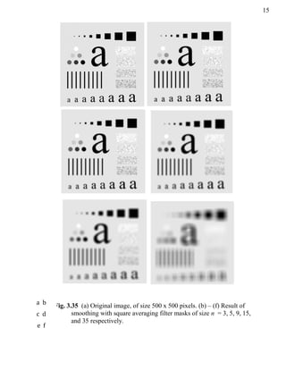
- 15. 14 3.6.1 Smoothing Linear Filters The commands, f = imread('Fig3.35(a).jpg'); w3 = 1/ (3. ^2)*ones (3); g3 = imfilter (f, w3, 'conv', 'replicate', 'same'); w5 = 1/ (5. ^2)*ones (5); g5 = imfilter (f, w5, 'conv', 'replicate', 'same'); w9 = 1/ (9. ^2)*ones (9); g9 = imfilter (f, w9, 'conv', 'replicate', 'same'); w15 = 1/ (15. ^2)*ones (15); g15 = imfilter (f, w15, 'conv', 'replicate', 'same'); w35 = 1/ (35. ^2)*ones (35); g35 = imfilter(f, w35, 'conv', 'replicate', 'same'); imshow (g3), figure, imshow (g5), figure, imshow (g9), figure, imshow (g15), figure, imshow (g35), figure; h = imread ('Fig3.36(a).jpg'); h15 = imfilter (h, w15, 'conv', 'replicate', 'same'); [m, n] = size (h15); for i = 1:m for j = 1:n if ((h15 (i,j)>=0) & (h15 (i,j)<128)) g (i,j) = 0; else g(i,j) = 255; end end end imshow(h15), figure, imshow(g);
- 16. 15 Fig. 3.35 (a) Original image, of size 500 x 500 pixels. (b) – (f) Result of smoothing with square averaging filter masks of size n = 3, 5, 9, 15, and 35 respectively. a b c d e f
- 17. 16 3.6.2 Order-Statistics Filters The commands, >> f = imread('Fig3.37(a).jpg'); w3 = 1/(3.^2)*ones(3); g3 = imfilter(f, w3, 'conv', 'replicate', 'same'); g = medfilt2(g3); imshow(g3), figure, imshow(g); a b c Fig. 3.36 (a) Original image. (b) Image processed by a 15 x 15 averaging mask. (c) Result of thresholding (b) Fig. 3.37 (a) X – ray image of circuit board corrupted by salt – and – pepper noise. (b) Noise reduction with a 3 x 3 averaging mask. (c) Noise reduction with a 3 x 3 median filter a b c
- 18. 17 3.7.2 The Laplacian The Laplacian for image enhancement is as follows: ( ) { ( ) ( ) ( ) ( ) ( ) The commands, % Laplacian function f1 = imread('Fig3.40(a).jpg'); w4 = fspecial('laplacian', 0); g1 = imfilter(f1, w4, 'replicate'); imshow(g1, [ ]), figure; f2 = im2double(f1); g2 = imfilter(f2, w4, 'replicate'); imshow(g2, [ ]), figure; g3 = imsubtract(f2,g2); imshow(g3) Fig. 3.40 (a) Image of the North Pole of the moon. (b) Laplacian image scaled for display purposes. (d) Image enhanced by Eq. (3.7 – 5) a b c d
- 19. 18 % Laplacian simplication f1 = imread ('Fig3.41(c).jpg'); w5 = [0 -1 0; -1 5 -1; 0 -1 0]; g1 = imfilter (f1, w5, 'replicate'); imshow (g1), figure; w9 = [-1 -1 -1; -1 9 -1; -1 -1 -1]; g2 = imfilter (f1, w9, 'replicate'); imshow (g2); 0 -1 0 -1 5 -1 0 -1 0 -1 -1 -1 -1 9 -1 -1 -1 -1 a b c d e Fig. 3.37 (a) Composite Laplacian mask. (b) A second composite mask. (c) Scanning electron microscope image. (d) and (e) Result of filtering with the masks in (a) and (b) respectively.
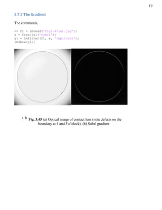
- 20. 19 3.7.3 The Gradient The commands, >> f1 = imread('Fig3.45(a).jpg'); w = fspecial('sobel'); g1 = imfilter(f1, w, 'replicate'); imshow(g1); a b Fig. 3.45 (a) Optical image of contact lens (note defects on the boundary at 4 and 5 o’clock). (b) Sobel gradient