Gradient boosting for regression problems with example basics of regression algorithm
0 likes147 views

The document discusses using gradient boosting for regression problems. Gradient boosting builds an additive model in a stage-wise fashion to minimize a loss function. It uses decision trees as weak learners that are added sequentially. The document demonstrates implementing gradient boosting in Python to predict Boston housing prices based on various attributes. It loads the dataset, trains a gradient boosting regressor model on 80% of the data, and evaluates the model on the remaining 20% with metrics showing good performance.
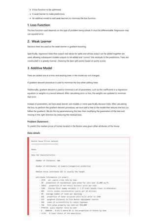
![The Boston house-price data has been used in many machine learning papers that address
regression problems.
Tools used:
Pandas
Numpy
Matplotlib
scikit-learn
Python Implementation with code :
Import necessary libraries
Import the necessary modules from specific libraries.
import numpy as np
import pandas as pd
%matplotlib inline
import matplotlib.pyplot as plt
from sklearn.model_selection import train_test_split
from sklearn import datasets
from sklearn.metrics import mean_squared_error
from sklearn import ensemble
Load the data set
Use the pandas module to read the taxi data from the file system. Check few records of the dataset.
#
#############################################################################
# Load data
boston = datasets.load_boston()
print(boston.data.shape, boston.target.shape)
print(boston.feature_names)
(506, 13) (506,)
['CRIM' 'ZN' 'INDUS' 'CHAS' 'NOX' 'RM' 'AGE' 'DIS' 'RAD' 'TAX' 'PTRATIO' 'B' 'LSTAT']
data = pd.DataFrame(boston.data,columns=boston.feature_names)
data = pd.concat([data,pd.Series(boston.target,name='MEDV')],axis=1)
data.head()
CRIM ZN INDUS CHAS NOX RM AGE DIS RAD TAX PTRATIO B LSTAT MEDV
0 0.00632 18.0 2.31 0.0 0.538 6.575 65.2 4.0900 1.0 296.0 15.3 396.90 4.98 24.0
1 0.02731 0.0 7.07 0.0 0.469 6.421 78.9 4.9671 2.0 242.0 17.8 396.90 9.14 21.6
2 0.02729 0.0 7.07 0.0 0.469 7.185 61.1 4.9671 2.0 242.0 17.8 392.83 4.03 34.7
- MEDV Median value of owner-occupied homes in $1000's
:Missing Attribute Values: None
:Creator: Harrison, D. and Rubinfeld, D.L.
This is a copy of UCI ML housing dataset.
http://archive.ics.uci.edu/ml/datasets/Housing
This dataset was taken from the StatLib library which is maintained at Carnegie Mellon University.
The Boston house-price data of Harrison, D. and Rubinfeld, D.L. 'Hedonic
prices and the demand for clean air', J. Environ. Economics & Management,
vol.5, 81-102, 1978. Used in Belsley, Kuh & Welsch, 'Regression diagnostics
...', Wiley, 1980. N.B. Various transformations are used in the table on
pages 244-261 of the latter.](https://image.slidesharecdn.com/gradientboostingforregressionproblemswithexamplebasicsofregressionalgorithm-181005085252/85/Gradient-boosting-for-regression-problems-with-example-basics-of-regression-algorithm-3-320.jpg)
![3 0.03237 0.0 2.18 0.0 0.458 6.998 45.8 6.0622 3.0 222.0 18.7 394.63 2.94 33.4
4 0.06905 0.0 2.18 0.0 0.458 7.147 54.2 6.0622 3.0 222.0 18.7 396.90 5.33 36.2
Select the predictor and target variables
X = data.iloc[:,:-1]
y = data.iloc[:,-1]
Train test split:
x_training_set, x_test_set, y_training_set, y_test_set = train_test_split(X,y,test_size=0.10,
random_state=42,
shuffle=True)
Training/model fitting:
Fit the model to selected supervised data
# Fit regression model
params = {'n_estimators': 500, 'max_depth': 4, 'min_samples_split': 2,
'learning_rate': 0.01, 'loss': 'ls'}
model = ensemble.GradientBoostingRegressor(**params)
model.fit(x_training_set, y_training_set)
Model parameters study :
from sklearn.metrics import mean_squared_error, r2_score
model_score = model.score(x_training_set,y_training_set)
# Have a look at R sq to give an idea of the fit ,
# Explained variance score: 1 is perfect prediction
print('R2 sq: ',model_score)
y_predicted = model.predict(x_test_set)
# The mean squared error
print("Mean squared error: %.2f"% mean_squared_error(y_test_set, y_predicted))
# Explained variance score: 1 is perfect prediction
print('Test Variance score: %.2f' % r2_score(y_test_set, y_predicted))
R2 sq: 0.9798997042218072
Mean squared error: 5.83
Test Variance score: 0.91
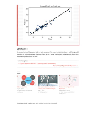
Accuracy report with test data :
Let’s visualize the goodness of the fit with the predictions being visualized by a line
# So let's run the model against the test data
from sklearn.model_selection import cross_val_predict
fig, ax = plt.subplots()
ax.scatter(y_test_set, y_predicted, edgecolors=(0, 0, 0))
ax.plot([y_test_set.min(), y_test_set.max()], [y_test_set.min(), y_test_set.max()], 'k--', lw=4)
ax.set_xlabel('Actual')
ax.set_ylabel('Predicted')
ax.set_title("Ground Truth vs Predicted")
plt.show()](https://image.slidesharecdn.com/gradientboostingforregressionproblemswithexamplebasicsofregressionalgorithm-181005085252/85/Gradient-boosting-for-regression-problems-with-example-basics-of-regression-algorithm-4-320.jpg)
Gradient boosting for regression problems with example basics of regression algorithm
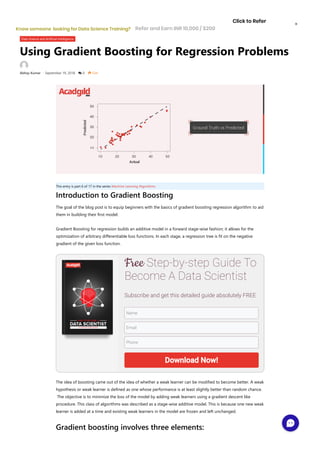
- 1. Using Gradient Boosting for Regression Problems Abhay Kumar • September 19, 2018 0 534 Data Science and Artificial Intelligence This entry is part 6 of 17 in the series Machine Learning Algorithms Introduction to Gradient Boosting The goal of the blog post is to equip beginners with the basics of gradient boosting regression algorithm to aid them in building their first model. Gradient Boosting for regression builds an additive model in a forward stage-wise fashion; it allows for the optimization of arbitrary differentiable loss functions. In each stage, a regression tree is fit on the negative gradient of the given loss function. The idea of boosting came out of the idea of whether a weak learner can be modified to become better. A weak hypothesis or weak learner is defined as one whose performance is at least slightly better than random chance. The objective is to minimize the loss of the model by adding weak learners using a gradient descent like procedure. This class of algorithms was described as a stage-wise additive model. This is because one new weak learner is added at a time and existing weak learners in the model are frozen and left unchanged. Gradient boosting involves three elements: Free Step-by-step Guide To Become A Data Scientist Subscribe and get this detailed guide absolutely FREE Name Email Phone Download Now! Refer and Earn INR 10,000 / $200 Click to Refer Know someone looking for Data Science Training? ×
- 2. A loss function to be optimized. A weak learner to make predictions. An additive model to add weak learners to minimize the loss function. 1. Loss Function The loss function used depends on the type of problem being solved. It must be differentiable. Regression may use squared error. 2. Weak Learner Decision trees are used as the weak learner in gradient boosting. Specifically, regression trees that output real values for splits and whose output can be added together are used, allowing subsequent models outputs to be added and “correct” the residuals in the predictions. Trees are constructed in a greedy manner, choosing the best split points based on purity scores. 3. Additive Model Trees are added one at a time, and existing trees in the model are not changed. A gradient descent procedure is used to minimize the loss when adding trees. Traditionally, gradient descent is used to minimize a set of parameters, such as the coefficients in a regression equation or weights in a neural network. After calculating error or loss, the weights are updated to minimize that error. Instead of parameters, we have weak learner sub-models or more specifically decision trees. After calculating the loss, to perform the gradient descent procedure, we must add a tree to the model that reduces the loss (i.e. follow the gradient). We do this by parameterizing the tree, then modifying the parameters of the tree and moving in the right direction by (reducing the residual loss). Problem Statement : To predict the median prices of homes located in the Boston area given other attributes of the house. Data details Boston House Prices dataset =========================== Notes ------ Data Set Characteristics: :Number of Instances: 506 :Number of Attributes: 13 numeric/categorical predictive :Median Value (attribute 14) is usually the target :Attribute Information (in order): - CRIM per capita crime rate by town - ZN proportion of residential land zoned for lots over 25,000 sq.ft. - INDUS proportion of non-retail business acres per town - CHAS Charles River dummy variable (= 1 if tract bounds river; 0 otherwise) - NOX nitric oxides concentration (parts per 10 million) - RM average number of rooms per dwelling - AGE proportion of owner-occupied units built prior to 1940 - DIS weighted distances to five Boston employment centres - RAD index of accessibility to radial highways - TAX full-value property-tax rate per $10,000 - PTRATIO pupil-teacher ratio by town - B 1000(Bk - 0.63)^2 where Bk is the proportion of blacks by town - LSTAT % lower status of the population
- 3. The Boston house-price data has been used in many machine learning papers that address regression problems. Tools used: Pandas Numpy Matplotlib scikit-learn Python Implementation with code : Import necessary libraries Import the necessary modules from specific libraries. import numpy as np import pandas as pd %matplotlib inline import matplotlib.pyplot as plt from sklearn.model_selection import train_test_split from sklearn import datasets from sklearn.metrics import mean_squared_error from sklearn import ensemble Load the data set Use the pandas module to read the taxi data from the file system. Check few records of the dataset. # ############################################################################# # Load data boston = datasets.load_boston() print(boston.data.shape, boston.target.shape) print(boston.feature_names) (506, 13) (506,) ['CRIM' 'ZN' 'INDUS' 'CHAS' 'NOX' 'RM' 'AGE' 'DIS' 'RAD' 'TAX' 'PTRATIO' 'B' 'LSTAT'] data = pd.DataFrame(boston.data,columns=boston.feature_names) data = pd.concat([data,pd.Series(boston.target,name='MEDV')],axis=1) data.head() CRIM ZN INDUS CHAS NOX RM AGE DIS RAD TAX PTRATIO B LSTAT MEDV 0 0.00632 18.0 2.31 0.0 0.538 6.575 65.2 4.0900 1.0 296.0 15.3 396.90 4.98 24.0 1 0.02731 0.0 7.07 0.0 0.469 6.421 78.9 4.9671 2.0 242.0 17.8 396.90 9.14 21.6 2 0.02729 0.0 7.07 0.0 0.469 7.185 61.1 4.9671 2.0 242.0 17.8 392.83 4.03 34.7 - MEDV Median value of owner-occupied homes in $1000's :Missing Attribute Values: None :Creator: Harrison, D. and Rubinfeld, D.L. This is a copy of UCI ML housing dataset. http://archive.ics.uci.edu/ml/datasets/Housing This dataset was taken from the StatLib library which is maintained at Carnegie Mellon University. The Boston house-price data of Harrison, D. and Rubinfeld, D.L. 'Hedonic prices and the demand for clean air', J. Environ. Economics & Management, vol.5, 81-102, 1978. Used in Belsley, Kuh & Welsch, 'Regression diagnostics ...', Wiley, 1980. N.B. Various transformations are used in the table on pages 244-261 of the latter.
- 4. 3 0.03237 0.0 2.18 0.0 0.458 6.998 45.8 6.0622 3.0 222.0 18.7 394.63 2.94 33.4 4 0.06905 0.0 2.18 0.0 0.458 7.147 54.2 6.0622 3.0 222.0 18.7 396.90 5.33 36.2 Select the predictor and target variables X = data.iloc[:,:-1] y = data.iloc[:,-1] Train test split: x_training_set, x_test_set, y_training_set, y_test_set = train_test_split(X,y,test_size=0.10, random_state=42, shuffle=True) Training/model fitting: Fit the model to selected supervised data # Fit regression model params = {'n_estimators': 500, 'max_depth': 4, 'min_samples_split': 2, 'learning_rate': 0.01, 'loss': 'ls'} model = ensemble.GradientBoostingRegressor(**params) model.fit(x_training_set, y_training_set) Model parameters study : from sklearn.metrics import mean_squared_error, r2_score model_score = model.score(x_training_set,y_training_set) # Have a look at R sq to give an idea of the fit , # Explained variance score: 1 is perfect prediction print('R2 sq: ',model_score) y_predicted = model.predict(x_test_set) # The mean squared error print("Mean squared error: %.2f"% mean_squared_error(y_test_set, y_predicted)) # Explained variance score: 1 is perfect prediction print('Test Variance score: %.2f' % r2_score(y_test_set, y_predicted)) R2 sq: 0.9798997042218072 Mean squared error: 5.83 Test Variance score: 0.91 Accuracy report with test data : Let’s visualize the goodness of the fit with the predictions being visualized by a line # So let's run the model against the test data from sklearn.model_selection import cross_val_predict fig, ax = plt.subplots() ax.scatter(y_test_set, y_predicted, edgecolors=(0, 0, 0)) ax.plot([y_test_set.min(), y_test_set.max()], [y_test_set.min(), y_test_set.max()], 'k--', lw=4) ax.set_xlabel('Actual') ax.set_ylabel('Predicted') ax.set_title("Ground Truth vs Predicted") plt.show()
- 5. This site uses Akismet to reduce spam. Learn how your comment data is processed. << Logistic Regression With PCA – Speeding Up and Benchmarking Random Forest Algorithm for Regression >> Conclusion : We can see that our R2 score and MSE are both very good. This means that we have found a well-fitting model to predict the median price value of a house. There can be a further improvement to the metric by doing some preprocessing before fitting the data. Series Navigation Related XGBoost Algorithm July 12, 2018 In "Data Science and Artificial Intelligence" Data Science Glossary- Machine Learning Tools and Terminologies May 3, 2018 In "All Categories" Random Forest Algorithm for Regression September 17, 2018 In "Data Science and Artificial Intelligence"