SlideShare a Scribd company logo
Chapter -3
Greedy Algorithms
“I always choose a lazy person to do a difficult job because he will
find an easy way to do it ”
Greedy Algorithm
• Solve problems with the simplest possible algorithm
• The hard part: showing that something simple actually works
• Pseudo-definition
– An algorithm is Greedy if it builds its solution by adding elements
one at a time using a simple rule
• Greedy is the most straight forward design technique.
• Most of the problems have n inputs and require us to obtain a subset
that satisfies some constraints.
• Any subset that satisfies these constraints is called a feasible solution.
• A feasible solution that does this is called an optimal solution.
• At each stage, a decision is made regarding whether or not a particular
input is in an optimal solution.
Greedy Algorithms
• A greedy algorithm is an approach for solving a problem by selecting
the best option available at the moment.
• It doesn't worry whether the current best result will bring the overall
optimal result.
• The algorithm never reverses the earlier decision even if the choice is
wrong. It works in a top-down approach.
• This algorithm may not produce the best result for all the problems.
It's because it always goes for the local best choice to produce the
global best result.
• However, we can determine if the algorithm can be used with any
problem if the problem has the following properties:
• If an optimal solution to the problem can be found by choosing the
best choice at each step without reconsidering the previous steps once
chosen, the problem can be solved using a greedy approach.
 This property is called greedy choice property.
2. Optimal Substructure
• If the optimal overall solution to the problem corresponds to the
optimal solution to its subproblems, then the problem can be solved
using a greedy approach.
 This property is called optimal substructure.
1. Greedy Choice Property
Advantages of Greedy Approach
 The algorithm is easier to describe.
 This algorithm can perform better than other algorithms (but, not in
all cases).
Drawback of Greedy Approach
• As mentioned earlier, the greedy algorithm doesn't always produce
the optimal solution. This is the major disadvantage of the algorithm
• For example, suppose we want to find the longest path in the graph
below from root to leaf. Let's use the greedy algorithm here.
Greedy Algorithm
Apply greedy approach to this tree to find the longest route
Greedy Approach
1. Let's start with the root node 20. The weight of the right child
is 3 and the weight of the left child is 2.
2. Our problem is to find the largest path. And, the optimal solution at
the moment is 3. So, the greedy algorithm will choose 3.
3. Finally the weight of an only child of 3 is 1. This gives us our final
result 20 + 3 + 1 = 24.
However, it is not the optimal solution. There is another path that
carries more weight (20 + 2 + 10 = 32) as shown in the image below.
Greedy Algorithm
Longest path
Therefore, greedy algorithms do not always give an optimal/feasible
solution.
Greedy Algorithm
 To begin with, the solution set (containing answers) is empty.
 At each step, an item is added to the solution set until a solution is
reached.
 If the solution set is feasible, the current item is kept.
 Else, the item is rejected and never considered again.
 Let's now use this algorithm to solve a problem.
Example - Greedy Approach
Problem: You have to make a change of an amount using the smallest possible number
of coins.
Amount: $18
Available coins are
$5 coin
$2 coin
$1 coin
There is no limit to the number of each coin you can use.
Solution:
1. Create an empty solution-set = { }. Available coins are {5, 2, 1}.
2. We are supposed to find the sum = 18. Let's start with sum = 0.
3. Always select the coin with the largest value (i.e. 5) until the sum > 18.
(When we select the largest value at each step, we hope to reach the
destination faster. This concept is called greedy choice property.)
4. In the first iteration, solution-set = {5} and sum = 5.
5. In the second iteration, solution-set = {5, 5} and sum = 10.
6. In the third iteration, solution-set = {5, 5, 5} and sum = 15.
7. In the fourth iteration, solution-set = {5, 5, 5, 2} and sum = 17. (We
cannot select 5 here because if we do so, sum = 20 which is greater than
18. So, we select the 2nd largest item which is 2.)
8. Similarly, in the fifth iteration, select 1. Now sum = 18 and solution-set =
{5, 5, 5, 2, 1}.
Some examples of greedy algorithms
Spanning tree
Huffman Coding
Dijkstra's Algorithm
Spanning Tree and Minimum Spanning Tree
• Before we learn about spanning trees, we need to understand two
graphs: undirected graphs and connected graphs.
• An undirected graph is a graph in which the edges do not point in
any direction (i.e. the edges are bidirectional).
Undirected Graph
Spanning Tree and Minimum Spanning Tree
• A connected graph is a graph in which there is always a path from a vertex
to any other vertex.
Connected graph
Spanning tree
• A spanning tree is a sub-graph of an undirected connected graph, which
includes all the vertices of the graph with a minimum possible number of
edges.
• If a vertex is missed, then it is not a spanning tree.
• The edges may or may not have weights assigned to them.
Spanning tree
• The total number of spanning trees with n vertices that can be created
from a complete graph is equal to n(n-2).
• If we have n = 4, the maximum number of possible spanning trees is
equal to 44-2 = 16. Thus, 16 spanning trees can be formed from a
complete graph with 4 vertices.
Example of a Spanning Tree
Let's understand the spanning tree with examples below:
Let the original graph be:
Normal graph
Spanning tree
• Some of the possible spanning trees that can be created from
the above graph are:
Minimum Spanning Tree
• A minimum spanning tree is a spanning tree in which the sum of
the weight of the edges is as minimum as possible.
Example of a Spanning Tree
• Let's understand the above definition with the help of the example
below.
• The initial graph is:
Weighted graph
The possible spanning trees from the above graph are:
Minimum Spanning Tree
• The minimum spanning tree from the above spanning trees is:
Minimum spanning tree
The minimum spanning tree from a graph is found using the following algorithms:
Prim's Algorithm
Kruskal's Algorithm
Spanning Tree Applications
 Computer Network Routing Protocol
 Cluster Analysis
 Civil Network Planning
Minimum Spanning tree Applications
 To find paths in the map
 To design networks like telecommunication networks, water supply networks, and
electrical grids.
Prim's Algorithm
Prim's algorithm is a minimum spanning tree algorithm that takes a graph as
input and finds the subset of the edges of that graph which
 Form a tree that includes every vertex
 Has the minimum sum of weights among all the trees that can be formed
from the graph
How Prim's algorithm works
It falls under a class of algorithms called greedy algorithms that find the local
optimum in the hopes of finding a global optimum.
We start from one vertex and keep adding edges with the lowest weight until
we reach our goal.
The steps for implementing Prim's algorithm are as follows:
Initialize the minimum spanning tree with a vertex chosen at random.
Find all the edges that connect the tree to new vertices, find the minimum and
add it to the tree
Keep repeating step 2 until we get a minimum spanning tree
Example of Prim's algorithm
Steps
Example of Prim's algorithm: steps
random
Example of Prim's algorithm: steps
Repeat until you have a spanning tree
Prim's Algorithm pseudocode
The pseudocode for prim's algorithm shows how we create two sets of vertices
U and V-U. U contains the list of vertices that have been visited and V-U the
list of vertices that haven't. One by one, we move vertices from set V-U to set
U by connecting the least weight edge.
Prim's Algorithm pseudocode
• T = ∅;
• U = { 1 };
• while (U ≠ V)
• let (u, v) be the lowest cost edge such that u ∈ U and v ∈ V - U;
• T = T ∪ {(u, v)}
• U = U ∪ {v}
Prim's vs Kruskal's Algorithm
• Kruskal's algorithm is another popular minimum spanning tree algorithm
that uses a different logic to find the MST of a graph.
• Instead of starting from a vertex, Kruskal's algorithm sorts all the edges
from low weight to high and keeps adding the lowest edges, ignoring those
edges that create a cycle.
Prim's Algorithm Complexity
• The time complexity of Prim's algorithm is O(E log V).
Prim's Algorithm Application
• Laying cables of electrical wiring
• In network designed
• To make protocols in network cycles
Huffman Coding
• Huffman Coding is a technique of compressing data to reduce its size
without losing any of the details. It was first developed by David
Huffman.
• Huffman Coding is generally useful to compress the data in which
there are frequently occurring characters.
• How Huffman Coding works?
• Suppose the string below is to be sent over a network.
Initial string
How Huffman Coding works?
• Each character occupies 8 bits. There are a total of 15 characters in the
above string. Thus, a total of 8 * 15 = 120 bits are required to send this
string.
• Using the Huffman Coding technique, we can compress the string to a
smaller size.
• Huffman coding first creates a tree using the frequencies of the character
and then generates code for each character.
• Once the data is encoded, it has to be decoded. Decoding is done using the
same tree.
• Huffman Coding prevents any ambiguity in the decoding process using the
concept of prefix code i.e. a code associated with a character should not
be present in the prefix of any other code. The tree created above helps in
maintaining the property.
How Huffman Coding works?
Huffman coding is done with the help of the following steps.
1.Calculate the frequency of each character in the string.
Frequency of string
2. Sort the characters in increasing order of the frequency. These are stored
in a priority queue Q.
Characters are sorted according to their ascending order frequency.
How Huffman Coding works?
3. Make each unique character as a leaf node.
4. Create an empty node z. Assign the minimum frequency to the left
child of z and assign the second minimum frequency to the right child
of z. Set the value of the z as the sum of the above two minimum
frequencies
getting the sum of the least numbers
How Huffman Coding works?
• Remove these two minimum frequencies from Q and add the sum into the
list of frequencies (* denote the internal nodes in the figure above).
• Insert node z into the tree.
• Repeat steps 3 to 5 for all the characters.
How Huffman Coding works?
• For each non-leaf node, assign 0 to the left edge and 1 to the right edge.
assign 0 to the left edge and 1 to the right edge
For sending the above string over a network, we have to send the tree as well as
the above compressed-code. The total size is given by the table below.
The total size is given by the table below.
Without encoding, the total size of the string was 120 bits. After encoding
the size is reduced to 32 + 15 + 28 = 75
Character Frequency Code Size
A 5 11 5*2 = 10
B 1 100 1*3 = 3
C 6 0 6*1 = 6
D 3 101 3*3 = 9
4 * 8 = 32 bits 15 bits 28 bits
.
How Huffman Coding works?
Decoding the code
• For decoding the code, we can take the code and traverse through the
tree to find the character.
• Let 101 is to be decoded, we can traverse from the root as in the figure
below.
Huffman Coding Algorithm
create a priority queue Q consisting of each unique character.
sort then in ascending order of their frequencies.
for all the unique characters:
create a newNode
extract minimum value from Q and assign it to leftChild of
newNode
extract minimum value from Q and assign it to rightChild of
newNode
calculate the sum of these two minimum values and assign it
to the value of newNode
insert this newNode into the tree
return rootNode
Huffman Coding Complexity
• The time complexity for encoding each unique character based on its
frequency is O(nlog n).
• Extracting minimum frequency from the priority queue takes
place 2*(n-1) times and its complexity is O(log n). Thus the overall
complexity is O(nlog n).
Huffman Coding Applications
• Huffman coding is used in conventional compression formats like
GZIP, BZIP2, PKZIP, etc.
• For text and fax transmissions.
Dijkstra's Algorithm
Dijkstra's algorithm allows us to find the shortest path between any two vertices of a
graph.
It differs from the minimum spanning tree because the shortest distance between two
vertices might not include all the vertices of the graph.
How Dijkstra's Algorithm works
Dijkstra's Algorithm works on the basis that any subpath B -> D of the shortest path A -
> D between vertices A and D is also the shortest path between vertices B and D.
How Dijkstra's Algorithm works
Each subpath is the shortest path
Djikstra used this property in the opposite direction i.e. we overestimate
the distance of each vertex from the starting vertex.
Then we visit each node and its neighbors to find the shortest subpath to
those neighbors.
The algorithm uses a greedy approach in the sense that we find the next
best solution hoping that the end result is the best solution for the whole
problem.
Example of Dijkstra's algorithm
s
Example of Dijkstra's algorithm
Djikstra's algorithm pseudocode
• We need to maintain the path distance of every vertex. We can store
that in an array of size v, where v is the number of vertices.
• We also want to be able to get the shortest path, not only know the
length of the shortest path. For this, we map each vertex to the vertex
that last updated its path length.
• Once the algorithm is over, we can backtrack from the destination
vertex to the source vertex to find the path.
• A minimum priority queue can be used to efficiently receive the
vertex with least path distance.
Djikstra's algorithm pseudocode
function dijkstra(G, S)
for each vertex V in G
distance[V] <- infinite
previous[V] <- NULL
If V != S, add V to Priority Queue Q
distance[S] <- 0
while Q IS NOT EMPTY
U <- Extract MIN from Q
for each unvisited neighbour V of U
tempDistance <- distance[U] + edge_weight(U, V)
if tempDistance < distance[V]
distance[V] <- tempDistance
previous[V] <- U
return distance[], previous[]
Code for Dijkstra's Algorithm
• The implementation of Dijkstra's Algorithm in C++ is given below.
The complexity of the code can be improved, but the abstractions are
convenient to relate the code with the algorithm.
Dijkstra's Algorithm Complexity
• Time Complexity: O(E Log V)
• where, E is the number of edges and V is the number of vertices.
• Space Complexity: O(V)
Dijkstra's Algorithm Applications
• To find the shortest path
• In social networking applications
• In a telephone network
• To find the locations in the map
Ad

Recommended

Aulas 11-guloso Algoritmos
Kevin Takano
 
Application of Dijkstra Algorithm in Robot path planning
Darling Jemima
 
Dijkstra.ppt
Dijkstra.ppt
Ruchika Sinha
 
Geométria computacional: Polígonos y-monótonos
Miguel Sancho
 
Welttierschutztag
Welttierschutztag
lilipuhi
 
Finite fields
Finite fields
BhumikaPal1
 
Epipolar geometry
Epipolar geometry
Safayet Hossain
 
Dynamic pgmming
Dynamic pgmming
Dr. C.V. Suresh Babu
 
Uninformed search /Blind search in AI
Kirti Verma
 
Minmax and alpha beta pruning.pptx
PriyadharshiniG41
 
AI Lecture 5 (game playing)
Tajim Md. Niamat Ullah Akhund
 
PROLOG: Database Manipulation In Prolog
DataminingTools Inc
 
Minimum spanning tree
Amit Kumar Rathi
 
Lecture 6 disjoint set
Abirami A
 
Hierarchical clustering of multi class data (the zoo dataset)
Raid Mahbouba
 
Lecture 25 hill climbing
Hema Kashyap
 
Solution of N Queens Problem genetic algorithm
MohammedAlKazal
 
Lecture 18 simplified memory bound a star algorithm
Hema Kashyap
 
Traveling salesman problem(tsp)
Viraj Patil
 
Maximum Matching in General Graphs
Ahmad Khayyat
 
Application of greedy method prim
Tech_MX
 
Adaptive Resonance Theory
surat murthy
 
AI3391 Artificial Intelligence Session 19 stochastics games.pptx
Guru Nanak Technical Institutions
 
Adjacency And Incidence Matrix
Abir Junayed
 
Subset sum problem(dp)
VishnuPratap7
 
Research Scope in Parallel Computing And Parallel Programming
Shitalkumar Sukhdeve
 
Lecture 6 expert systems
Vajira Thambawita
 
Androidアプリ本格開発入門 webブラウザ編
bg1 333
 
Unit3_1.pdf
Unit3_1.pdf
Pratimakumari213460
 
7. Algorithm Design and analysis ppt.pptx
deivasigamani9
 

More Related Content

What's hot (20)

Uninformed search /Blind search in AI
Kirti Verma
 
Minmax and alpha beta pruning.pptx
PriyadharshiniG41
 
AI Lecture 5 (game playing)
Tajim Md. Niamat Ullah Akhund
 
PROLOG: Database Manipulation In Prolog
DataminingTools Inc
 
Minimum spanning tree
Amit Kumar Rathi
 
Lecture 6 disjoint set
Abirami A
 
Hierarchical clustering of multi class data (the zoo dataset)
Raid Mahbouba
 
Lecture 25 hill climbing
Hema Kashyap
 
Solution of N Queens Problem genetic algorithm
MohammedAlKazal
 
Lecture 18 simplified memory bound a star algorithm
Hema Kashyap
 
Traveling salesman problem(tsp)
Viraj Patil
 
Maximum Matching in General Graphs
Ahmad Khayyat
 
Application of greedy method prim
Tech_MX
 
Adaptive Resonance Theory
surat murthy
 
AI3391 Artificial Intelligence Session 19 stochastics games.pptx
Guru Nanak Technical Institutions
 
Adjacency And Incidence Matrix
Abir Junayed
 
Subset sum problem(dp)
VishnuPratap7
 
Research Scope in Parallel Computing And Parallel Programming
Shitalkumar Sukhdeve
 
Lecture 6 expert systems
Vajira Thambawita
 
Androidアプリ本格開発入門 webブラウザ編
bg1 333
 
Uninformed search /Blind search in AI
Kirti Verma
 
Minmax and alpha beta pruning.pptx
PriyadharshiniG41
 
PROLOG: Database Manipulation In Prolog
DataminingTools Inc
 
Lecture 6 disjoint set
Abirami A
 
Hierarchical clustering of multi class data (the zoo dataset)
Raid Mahbouba
 
Lecture 25 hill climbing
Hema Kashyap
 
Solution of N Queens Problem genetic algorithm
MohammedAlKazal
 
Lecture 18 simplified memory bound a star algorithm
Hema Kashyap
 
Traveling salesman problem(tsp)
Viraj Patil
 
Maximum Matching in General Graphs
Ahmad Khayyat
 
Application of greedy method prim
Tech_MX
 
Adaptive Resonance Theory
surat murthy
 
AI3391 Artificial Intelligence Session 19 stochastics games.pptx
Guru Nanak Technical Institutions
 
Adjacency And Incidence Matrix
Abir Junayed
 
Subset sum problem(dp)
VishnuPratap7
 
Research Scope in Parallel Computing And Parallel Programming
Shitalkumar Sukhdeve
 
Androidアプリ本格開発入門 webブラウザ編
bg1 333
 

Similar to Greedy algorithm pptxe file for computer (20)

Unit3_1.pdf
Unit3_1.pdf
Pratimakumari213460
 
7. Algorithm Design and analysis ppt.pptx
deivasigamani9
 
Mastering Greedy Algorithms: Optimizing Solutions for Efficiency"
22bcs058
 
Lec07-Greedy Algorithms.pdf Lec07-Greedy Algorithms.pdf
MAJDABDALLAH3
 
3 Greedy-lec.pptggggghhhhhhhyyyyyyyyyyyyyy
esraelman182
 
greedy algorithm.pptx good for understanding
HUSNAINAHMAD39
 
Greedy Algorihm
Greedy Algorihm
Muhammad Amjad Rana
 
Module 2 - Greedy Algorithm Data structures and algorithm
farzanirani201402
 
Undecidable Problems - COPING WITH THE LIMITATIONS OF ALGORITHM POWER
muthukrishnavinayaga
 
Single source Shortest path algorithm with example
VINITACHAUHAN21
 
Greedy Method unit-2(Design and analysis of algorithms).pptx
shivani366010
 
Data Analysis and Algorithms Lecture 1: Introduction
TayyabSattar5
 
Undecidable Problems and Approximation Algorithms
Muthu Vinayagam
 
Lecture-11-CS345A-2023 of Design and Analysis
ssuser9183b6
 
Greedy algorithm
Greedy algorithm
International Islamic University
 
Greedy Algorithms
Greedy Algorithms
Amrinder Arora
 
Greedy Algorithm
Greedy Algorithm
Waqar Akram
 
Greedy technique - Algorithm design techniques using data structures
divyammo
 
Minimum Spanning Tree.pptx
HrRajon2
 
Daa chapter4
Daa chapter4
B.Kirron Reddi
 
7. Algorithm Design and analysis ppt.pptx
deivasigamani9
 
Mastering Greedy Algorithms: Optimizing Solutions for Efficiency"
22bcs058
 
Lec07-Greedy Algorithms.pdf Lec07-Greedy Algorithms.pdf
MAJDABDALLAH3
 
3 Greedy-lec.pptggggghhhhhhhyyyyyyyyyyyyyy
esraelman182
 
greedy algorithm.pptx good for understanding
HUSNAINAHMAD39
 
Module 2 - Greedy Algorithm Data structures and algorithm
farzanirani201402
 
Undecidable Problems - COPING WITH THE LIMITATIONS OF ALGORITHM POWER
muthukrishnavinayaga
 
Single source Shortest path algorithm with example
VINITACHAUHAN21
 
Greedy Method unit-2(Design and analysis of algorithms).pptx
shivani366010
 
Data Analysis and Algorithms Lecture 1: Introduction
TayyabSattar5
 
Undecidable Problems and Approximation Algorithms
Muthu Vinayagam
 
Lecture-11-CS345A-2023 of Design and Analysis
ssuser9183b6
 
Greedy Algorithm
Greedy Algorithm
Waqar Akram
 
Greedy technique - Algorithm design techniques using data structures
divyammo
 
Minimum Spanning Tree.pptx
HrRajon2
 
Ad

Recently uploaded (20)

FLOURISHING THROUGH SENSES: FROM Ab‘SENSE’ to Pre‘SENSE’ to Es‘SENSE’ to Re-...
Samuel Thuo
 
Chapter 5 - 1.ppt,Chapter 5 - 1.ppt,Chapter 5 - 1.ppt
NaveedRehman55
 
Chapter 3 Agile Development 7e.ppt,Chapter 5 - 1.ppt
NaveedRehman55
 
AI-Driven-Personalization-in-UX-Designing-for-One-in-a-Million.pdf
Sultan Shalakhti
 
Numbers 1 to 100 Circle Flashcard s.pptx
KarenGimena1
 
Assignment 1_ studying a roomkjdhfkeqjdhfjeqhfdjkqebf
kunduanannya2003
 
I2C EEPROM SIMULATION IN VERILOG-12.pptx
sudheerkurakula1218
 
User Persona for a fitness CEO Founder
modele dawodu
 
Transformative Storytelling_ Insights from the Sankofa Writing Intensive.pdf
Dr. Rema
 
Formal Informal Apology letter.pptxvvvvv
iqlimajurayeva
 
AVA-fundamentals-Gavin-Ambrose-Paul-Harris-The-fundamentals-of-typography-AVA...
FaisalNurWibowo
 
Bethany Michels Master of Architecture Thesis 2025
Bethany Michels
 
Exploratory Experiences Built by Design (UXPA25)
Design for Context
 
Presentation.pptx tinkercadjajsjhdhdhdhs
sukh27012
 
最新版美国威斯康星大学普拉特维尔分校毕业证(UWP毕业证书)原版定制
taqyea
 
Capcut Pro Crack For PC Latest Version {Fully Unlocked}
Ayesha khan
 
Indian_Constitution_Presentation.pptx , images
jaglandushyant
 
Canva Pro Crack Free Download 2025 Latest
chandchuhdary068
 
week3.pptx python related programs and outputs
doramira833
 
最新版美国北密歇根大学毕业证(NMU毕业证书)原版定制
Taqyea
 
Ad

Greedy algorithm pptxe file for computer

  • 1. Chapter -3 Greedy Algorithms “I always choose a lazy person to do a difficult job because he will find an easy way to do it ”
  • 2. Greedy Algorithm • Solve problems with the simplest possible algorithm • The hard part: showing that something simple actually works • Pseudo-definition – An algorithm is Greedy if it builds its solution by adding elements one at a time using a simple rule • Greedy is the most straight forward design technique. • Most of the problems have n inputs and require us to obtain a subset that satisfies some constraints. • Any subset that satisfies these constraints is called a feasible solution. • A feasible solution that does this is called an optimal solution. • At each stage, a decision is made regarding whether or not a particular input is in an optimal solution.
  • 3. Greedy Algorithms • A greedy algorithm is an approach for solving a problem by selecting the best option available at the moment. • It doesn't worry whether the current best result will bring the overall optimal result. • The algorithm never reverses the earlier decision even if the choice is wrong. It works in a top-down approach. • This algorithm may not produce the best result for all the problems. It's because it always goes for the local best choice to produce the global best result. • However, we can determine if the algorithm can be used with any problem if the problem has the following properties:
  • 4. • If an optimal solution to the problem can be found by choosing the best choice at each step without reconsidering the previous steps once chosen, the problem can be solved using a greedy approach.  This property is called greedy choice property. 2. Optimal Substructure • If the optimal overall solution to the problem corresponds to the optimal solution to its subproblems, then the problem can be solved using a greedy approach.  This property is called optimal substructure. 1. Greedy Choice Property
  • 5. Advantages of Greedy Approach  The algorithm is easier to describe.  This algorithm can perform better than other algorithms (but, not in all cases). Drawback of Greedy Approach • As mentioned earlier, the greedy algorithm doesn't always produce the optimal solution. This is the major disadvantage of the algorithm • For example, suppose we want to find the longest path in the graph below from root to leaf. Let's use the greedy algorithm here.
  • 6. Greedy Algorithm Apply greedy approach to this tree to find the longest route Greedy Approach 1. Let's start with the root node 20. The weight of the right child is 3 and the weight of the left child is 2. 2. Our problem is to find the largest path. And, the optimal solution at the moment is 3. So, the greedy algorithm will choose 3. 3. Finally the weight of an only child of 3 is 1. This gives us our final result 20 + 3 + 1 = 24. However, it is not the optimal solution. There is another path that carries more weight (20 + 2 + 10 = 32) as shown in the image below.
  • 7. Greedy Algorithm Longest path Therefore, greedy algorithms do not always give an optimal/feasible solution.
  • 8. Greedy Algorithm  To begin with, the solution set (containing answers) is empty.  At each step, an item is added to the solution set until a solution is reached.  If the solution set is feasible, the current item is kept.  Else, the item is rejected and never considered again.  Let's now use this algorithm to solve a problem. Example - Greedy Approach Problem: You have to make a change of an amount using the smallest possible number of coins. Amount: $18 Available coins are $5 coin $2 coin $1 coin There is no limit to the number of each coin you can use.
  • 9. Solution: 1. Create an empty solution-set = { }. Available coins are {5, 2, 1}. 2. We are supposed to find the sum = 18. Let's start with sum = 0. 3. Always select the coin with the largest value (i.e. 5) until the sum > 18. (When we select the largest value at each step, we hope to reach the destination faster. This concept is called greedy choice property.) 4. In the first iteration, solution-set = {5} and sum = 5. 5. In the second iteration, solution-set = {5, 5} and sum = 10. 6. In the third iteration, solution-set = {5, 5, 5} and sum = 15. 7. In the fourth iteration, solution-set = {5, 5, 5, 2} and sum = 17. (We cannot select 5 here because if we do so, sum = 20 which is greater than 18. So, we select the 2nd largest item which is 2.) 8. Similarly, in the fifth iteration, select 1. Now sum = 18 and solution-set = {5, 5, 5, 2, 1}.
  • 10. Some examples of greedy algorithms Spanning tree Huffman Coding Dijkstra's Algorithm
  • 11. Spanning Tree and Minimum Spanning Tree • Before we learn about spanning trees, we need to understand two graphs: undirected graphs and connected graphs. • An undirected graph is a graph in which the edges do not point in any direction (i.e. the edges are bidirectional). Undirected Graph
  • 12. Spanning Tree and Minimum Spanning Tree • A connected graph is a graph in which there is always a path from a vertex to any other vertex. Connected graph Spanning tree • A spanning tree is a sub-graph of an undirected connected graph, which includes all the vertices of the graph with a minimum possible number of edges. • If a vertex is missed, then it is not a spanning tree. • The edges may or may not have weights assigned to them.
  • 13. Spanning tree • The total number of spanning trees with n vertices that can be created from a complete graph is equal to n(n-2). • If we have n = 4, the maximum number of possible spanning trees is equal to 44-2 = 16. Thus, 16 spanning trees can be formed from a complete graph with 4 vertices. Example of a Spanning Tree Let's understand the spanning tree with examples below: Let the original graph be: Normal graph
  • 14. Spanning tree • Some of the possible spanning trees that can be created from the above graph are:
  • 15. Minimum Spanning Tree • A minimum spanning tree is a spanning tree in which the sum of the weight of the edges is as minimum as possible. Example of a Spanning Tree • Let's understand the above definition with the help of the example below. • The initial graph is: Weighted graph The possible spanning trees from the above graph are:
  • 17. Minimum Spanning Tree • The minimum spanning tree from the above spanning trees is: Minimum spanning tree The minimum spanning tree from a graph is found using the following algorithms: Prim's Algorithm Kruskal's Algorithm Spanning Tree Applications  Computer Network Routing Protocol  Cluster Analysis  Civil Network Planning Minimum Spanning tree Applications  To find paths in the map  To design networks like telecommunication networks, water supply networks, and electrical grids.
  • 18. Prim's Algorithm Prim's algorithm is a minimum spanning tree algorithm that takes a graph as input and finds the subset of the edges of that graph which  Form a tree that includes every vertex  Has the minimum sum of weights among all the trees that can be formed from the graph How Prim's algorithm works It falls under a class of algorithms called greedy algorithms that find the local optimum in the hopes of finding a global optimum. We start from one vertex and keep adding edges with the lowest weight until we reach our goal. The steps for implementing Prim's algorithm are as follows: Initialize the minimum spanning tree with a vertex chosen at random. Find all the edges that connect the tree to new vertices, find the minimum and add it to the tree Keep repeating step 2 until we get a minimum spanning tree
  • 19. Example of Prim's algorithm Steps
  • 20. Example of Prim's algorithm: steps random
  • 21. Example of Prim's algorithm: steps Repeat until you have a spanning tree Prim's Algorithm pseudocode The pseudocode for prim's algorithm shows how we create two sets of vertices U and V-U. U contains the list of vertices that have been visited and V-U the list of vertices that haven't. One by one, we move vertices from set V-U to set U by connecting the least weight edge.
  • 22. Prim's Algorithm pseudocode • T = ∅; • U = { 1 }; • while (U ≠ V) • let (u, v) be the lowest cost edge such that u ∈ U and v ∈ V - U; • T = T ∪ {(u, v)} • U = U ∪ {v} Prim's vs Kruskal's Algorithm • Kruskal's algorithm is another popular minimum spanning tree algorithm that uses a different logic to find the MST of a graph. • Instead of starting from a vertex, Kruskal's algorithm sorts all the edges from low weight to high and keeps adding the lowest edges, ignoring those edges that create a cycle.
  • 23. Prim's Algorithm Complexity • The time complexity of Prim's algorithm is O(E log V). Prim's Algorithm Application • Laying cables of electrical wiring • In network designed • To make protocols in network cycles
  • 24. Huffman Coding • Huffman Coding is a technique of compressing data to reduce its size without losing any of the details. It was first developed by David Huffman. • Huffman Coding is generally useful to compress the data in which there are frequently occurring characters. • How Huffman Coding works? • Suppose the string below is to be sent over a network. Initial string
  • 25. How Huffman Coding works? • Each character occupies 8 bits. There are a total of 15 characters in the above string. Thus, a total of 8 * 15 = 120 bits are required to send this string. • Using the Huffman Coding technique, we can compress the string to a smaller size. • Huffman coding first creates a tree using the frequencies of the character and then generates code for each character. • Once the data is encoded, it has to be decoded. Decoding is done using the same tree. • Huffman Coding prevents any ambiguity in the decoding process using the concept of prefix code i.e. a code associated with a character should not be present in the prefix of any other code. The tree created above helps in maintaining the property.
  • 26. How Huffman Coding works? Huffman coding is done with the help of the following steps. 1.Calculate the frequency of each character in the string. Frequency of string 2. Sort the characters in increasing order of the frequency. These are stored in a priority queue Q. Characters are sorted according to their ascending order frequency.
  • 27. How Huffman Coding works? 3. Make each unique character as a leaf node. 4. Create an empty node z. Assign the minimum frequency to the left child of z and assign the second minimum frequency to the right child of z. Set the value of the z as the sum of the above two minimum frequencies getting the sum of the least numbers
  • 28. How Huffman Coding works? • Remove these two minimum frequencies from Q and add the sum into the list of frequencies (* denote the internal nodes in the figure above). • Insert node z into the tree. • Repeat steps 3 to 5 for all the characters.
  • 29. How Huffman Coding works? • For each non-leaf node, assign 0 to the left edge and 1 to the right edge. assign 0 to the left edge and 1 to the right edge For sending the above string over a network, we have to send the tree as well as the above compressed-code. The total size is given by the table below.
  • 30. The total size is given by the table below. Without encoding, the total size of the string was 120 bits. After encoding the size is reduced to 32 + 15 + 28 = 75 Character Frequency Code Size A 5 11 5*2 = 10 B 1 100 1*3 = 3 C 6 0 6*1 = 6 D 3 101 3*3 = 9 4 * 8 = 32 bits 15 bits 28 bits .
  • 31. How Huffman Coding works? Decoding the code • For decoding the code, we can take the code and traverse through the tree to find the character. • Let 101 is to be decoded, we can traverse from the root as in the figure below.
  • 32. Huffman Coding Algorithm create a priority queue Q consisting of each unique character. sort then in ascending order of their frequencies. for all the unique characters: create a newNode extract minimum value from Q and assign it to leftChild of newNode extract minimum value from Q and assign it to rightChild of newNode calculate the sum of these two minimum values and assign it to the value of newNode insert this newNode into the tree return rootNode
  • 33. Huffman Coding Complexity • The time complexity for encoding each unique character based on its frequency is O(nlog n). • Extracting minimum frequency from the priority queue takes place 2*(n-1) times and its complexity is O(log n). Thus the overall complexity is O(nlog n). Huffman Coding Applications • Huffman coding is used in conventional compression formats like GZIP, BZIP2, PKZIP, etc. • For text and fax transmissions.
  • 34. Dijkstra's Algorithm Dijkstra's algorithm allows us to find the shortest path between any two vertices of a graph. It differs from the minimum spanning tree because the shortest distance between two vertices might not include all the vertices of the graph. How Dijkstra's Algorithm works Dijkstra's Algorithm works on the basis that any subpath B -> D of the shortest path A - > D between vertices A and D is also the shortest path between vertices B and D.
  • 35. How Dijkstra's Algorithm works Each subpath is the shortest path Djikstra used this property in the opposite direction i.e. we overestimate the distance of each vertex from the starting vertex. Then we visit each node and its neighbors to find the shortest subpath to those neighbors. The algorithm uses a greedy approach in the sense that we find the next best solution hoping that the end result is the best solution for the whole problem.
  • 36. Example of Dijkstra's algorithm s
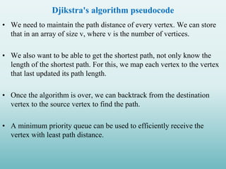
  • 40. Djikstra's algorithm pseudocode • We need to maintain the path distance of every vertex. We can store that in an array of size v, where v is the number of vertices. • We also want to be able to get the shortest path, not only know the length of the shortest path. For this, we map each vertex to the vertex that last updated its path length. • Once the algorithm is over, we can backtrack from the destination vertex to the source vertex to find the path. • A minimum priority queue can be used to efficiently receive the vertex with least path distance.
  • 41. Djikstra's algorithm pseudocode function dijkstra(G, S) for each vertex V in G distance[V] <- infinite previous[V] <- NULL If V != S, add V to Priority Queue Q distance[S] <- 0 while Q IS NOT EMPTY U <- Extract MIN from Q for each unvisited neighbour V of U tempDistance <- distance[U] + edge_weight(U, V) if tempDistance < distance[V] distance[V] <- tempDistance previous[V] <- U return distance[], previous[]
  • 42. Code for Dijkstra's Algorithm • The implementation of Dijkstra's Algorithm in C++ is given below. The complexity of the code can be improved, but the abstractions are convenient to relate the code with the algorithm. Dijkstra's Algorithm Complexity • Time Complexity: O(E Log V) • where, E is the number of edges and V is the number of vertices. • Space Complexity: O(V) Dijkstra's Algorithm Applications • To find the shortest path • In social networking applications • In a telephone network • To find the locations in the map