High-dimensional polytopes defined by oracles: algorithms, computations and applications

High-dimensional polytopes deﬁned by oracles:
algorithms, computations and applications
Vissarion Fisikopoulos
Dept. of Informatics & Telecommunications, University of Athens
PhD defence, Athens, 24.Apr.2014

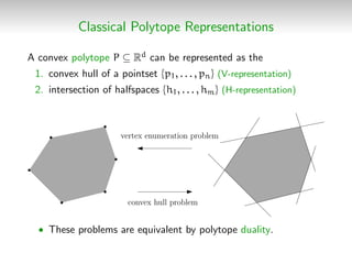
Classical Polytope Representations
A convex polytope P ⊆ Rd can be represented as the
1. convex hull of a pointset {p1, . . . , pn} (V-representation)
2. intersection of halfspaces {h1, . . . , hm} (H-representation)
convex hull problem
vertex enumeration problem
• These problems are equivalent by polytope duality.

Algorithmic Issues
• For general dimension d there is no polynomial algorithm for
the convex hull (or vertex enumeration) problem since m can
be O n d/2 [McMullen’70].
• It is open whether there exist a total poly-time algorithm for
the convex hull (or vertex enumeration) problem, i.e. runs in
poly-time in n, m, d.

Polytope Oracles
Implicit representation for a polytope P ⊆ Rd.
OPTP: Given direction c ∈ Rd return the vertex v ∈ P that maximizes
cT v.
SEPP: Given point y ∈ Rd, return yes if y ∈ P otherwise a
hyperplane h that separates y from P.
c
v
P P
h
y

Why polytope Oracles?
• Polynomial time algorithms for combinatorial optimization
problems using the ellipsoid method
[Grötschel-Lovász-Schrijver’93]
• Randomized polynomial-time algorithms for approximating the
volume of convex bodies
[Dyer-Frieze-Kannan ’90],. . . ,[Lovász-Vempala ’04]

Our view of the Oracles
Resultant, Discriminant, Secondary polytopes
• Vertices → subdivisions of a
pointset’s convex hull
• OPTP is available via a subdivision
computation
• Applications in Computational Algebraic Geometry, Geometric
Modelling, Optimization, Combinatorics

Main actor: resultant polytope
• Geometry: Minkowski summands of secondary polytopes,
generalize Birkhoﬀ polytopes
• Algebra: resultant expresses the solvability of polynomial
systems
• Applications: resultant computation, implicitization of
parametric hypersurfaces [Emiris, Kalinka, Konaxis, LuuBa ’12]
Enneper’s Minimal Surface

Polytopes and Algebra
• Given n + 1 polynomials on n variables.
f0(x) = ax2
+ b
f1(x) = cx2
+ dx + e

• Supports (set of exponents of monomials with non-zero
coeﬃcient) A0, A1, . . . , An ⊂ Zn.
A0
A1
f0(x) = ax2
+ b
f1(x) = cx2
+ dx + e

• The resultant R is the polynomial in the coeﬃcients of a
system of polynomials which vanishes if there exists a
common root in the torus of the given polynomials.
A0
A1
R(a, b, c, d, e) = ad2
b + c2
b2
− 2caeb + a2
e2
f0(x) = ax2
+ b
f1(x) = cx2
+ dx + e

• The resultant R is the polynomial in the coeﬃcients of a
system of polynomials which vanishes if there exists a
common root in the torus of the given polynomials.
• The resultant polytope N(R), is the convex hull of the
support of R, i.e. the Newton polytope of the resultant.
A0
A1
N(R)R(a, b, c, d, e) = ad2
b + c2
b2
− 2caeb + a2
e2
f0(x) = ax2
+ b
f1(x) = cx2
+ dx + e

Mixed subdivisions
A subdivision S of Minkowski sum A0 + A1 + · · · + An is
• mixed: cells are Minkowski sums of subsets of Ai’s,
• ﬁne: for each cell σ = σ0 + · · · + σn, dim(σ) = n
i=0 dim(σi)
Example
A0
A1
A2 ﬁne mixed subdivision S of A0 + A1 + A2

Resultant polytope vertices
Theorem [GKZ’94,
Sturmfels’94]
• many-to-one relation from
regular ﬁne mixed
subdivisions of
A0 + · · · + An to N(R)
vertices
• one-to-one relation between
regular ﬁne mixed
subdivisions and secondary
polytope Σ vertices

The idea of the algorithm
Input: A0, A1, . . . , An ⊂ Zn
Simplistic method:
• compute the vertices of secondary polytope Σ [Rambau ’02]
• many-to-one relation between vertices of Σ and N(R)

The idea of the algorithm
Input: A0, A1, . . . , An ⊂ Zn
New Algorithm:
• Optimization oracle for N(R) by subdivision computation
• Output sensitive: 1 subd. per N(R) vertex + 1 per N(R) facet
• Computes projections of N(R), Σ

The Algorithm
• incremental
• ﬁrst: compute conv.hull of d + 1 aﬀ. indep. vertices of N(R)
• step: call the oracle with outer normal vector of a halfspace
→ either validate this halfspace
→ or add a new vertex to the convex hull
N(R)
Q

The Algorithm
• incremental
Theorem
H-, V-repr. & triang. T of N(R) can be computed in
O(d5
ns2
) arithmetic operations + O(n + m) oracle calls
n, m, s are the number of vertices, facets of N(R), cells of T resp.

The Algorithm
• incremental
Theorem
H-, V-repr. & triang. T of N(R) can be computed in
O(d5
ns2
) arithmetic operations + O(n + m) oracle calls
n, m, s are the number of vertices, facets of N(R), cells of T resp.
BUT: s can be O n d/2

ResPol package
• C++
• Towards high-dimensional
• Propose hashing of determinantal predicates scheme:
optimizing sequences of similar determinants (x100 speed-up)
• Computes 5-, 6- and 7-dimensional polytopes with 35K, 23K
and 500 vertices, respectively, within 2hrs
• Computes polytopes of many important surface equations
encountered in geometric modeling in < 1sec, whereas the
corresponding secondary polytopes are intractable

References
• Emiris, F, Konaxis, Peñaranda An output-sensitive algorithm
for computing projections of resultant polytopes. Proc. of
28th ACM Annual Symposium on Computational Geometry,
2012, Chapel Hill, NC, USA.
• Emiris, F, Konaxis, Peñaranda An oracle-based, output
sensitive algorithm for projections of resultant polytopes.
International Journal of Computational Geometry and
Applications (Special issue) World Scientific.

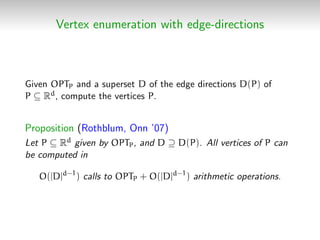
Vertex enumeration with edge-directions
Given OPTP and a superset D of the edge directions D(P) of
P ⊆ Rd, compute the vertices P.
Proposition (Rothblum, Onn ’07)
Let P ⊆ Rd given by OPTP, and D ⊇ D(P). All vertices of P can
be computed in
O(|D|d−1
) calls to OPTP + O(|D|d−1
) arithmetic operations.

Well-described polytopes and oracles
Deﬁnition
A polytope P ⊆ Rd is well-described (with a parameter ϕ) if there
exists an H-representation for P in which every inequality has
encoding length at most ϕ. The encoding length of P is
P = d + ϕ.
Proposition (Gr¨otschel et al.’93)
For a well-described polytope, we can compute OPTP from SEPP
(and vice versa) in oracle polynomial-time. The runtime
(polynomially) depends on d and ϕ.

The edge-skeleton algorithm
Input:
• OPTP
• Edge vec. P (dir. & len.): D
Output:
• Edge-skeleton of P
P
c
Sketch of Algorithm:
• Compute a vertex of P (x = OPTP(c) for arbitrary cT ∈ Rd)

Input:
• OPTP
Output:
P
• Compute segments S = {(x, x + d), for all d ∈ D}

Input:
• OPTP
Output:
P
• Remove from S all segments (x, y) s.t. y /∈ P (OPTP → SEPP)

Input:
• OPTP
Output:
P
• Remove from S the segments that are not extreme

Input:
• OPTP
Output:
P
• Remove from S the segments that are not extreme
Can be altered to work with edge directions only

Complexity
Theorem
Given OPTP and a superset of edge directions D of a well-
described polytope P ⊆ Rd, the edge skeleton of P can be
computed in oracle total polynomial-time
O n|D| T + LP(d3
|D| B ) + d log n ,
• n the number of vertices of P,
• T : runtime of oracle conversion algorithm for P and D,
• B is the binary encoding length of the vector set P and D,
• LP( A + b + c ) runtime of max cT x over {x : Ax ≤ b}.

Applications
Corollary
The edge skeleton of resultant, secondary polytopes can be
computed in oracle total polynomial-time.
Corollary
The edge skeletons of polytopes appearing in convex combinatorial
optimization [Rothblum-Onn ’04] and convex integer
programming [De Loera et al. ’09] problems can be computed in
oracle total polynomial-time.

References
• Emiris, F, Gärtner Efficient Volume and Edge-Skeleton
Computation for Polytopes Given by Oracles. Proc. of 29th
European Workshop on Computational Geometry,
Braunschweig, Germany 2013.
• Emiris, F, Gärtner Efficient edge skeleton computation for
polytopes defined by oracles. Submitted to Computational
Geometry - Theory and Applications.

The volume computation problem
Input: Polytope P := {x ∈ Rd | Ax ≤ b} A ∈ Rm×d, b ∈ Rm
Output: Volume of P
• #-P hard for vertex and for halfspace repres. [DyerFrieze’88]

Output: Volume of P
• randomized poly-time algorithm approximates the volume of a
convex body with high probability and arbitrarily small relative
error [DyerFriezeKannan’91] O∗(d23) → O∗(d4) [LovVemp’04]

Output: Volume of P
• randomized poly-time algorithm approximates the volume of a
convex body with high probability and arbitrarily small relative
error [DyerFriezeKannan’91] O∗(d23) → O∗(d4) [LovVemp’04]
Implementations
• Exact (VINCI, Qhull, etc.) cannot compute in high
dimensions (e.g. > 20)
• Randomized ([CousinsVempala’14], [EmirisF’14]) compute in
high dimensions (e.g. 100)

How do we compute a random point in a polytope P?
• easy for simple shapes like simplex or cube

How do we compute a random point in a polytope P?
• easy for simple shapes like simplex or cube
• BUT for arbitrary polytopes we need random walks

Random Directions Hit-and-Run (RDHR)
x
P
B
Input: point x ∈ P
Output: new point x ∈ P
1. line through x, uniform on B(x, 1)
2. set x to be a uniform disrtibuted
point on P ∩
Iterate this for W steps.

x
P
point on P ∩

xP
point on P ∩
• x is unif. random distrib. in P after W = O∗(d3) steps,
where O∗(·) hides log factors [LovaszVempala’06]
• to generate many random points iterate this procedure

Multiphase Monte Carlo (Sequence of balls)
B = B(c, r)
B = B(c, ρ)
P
• B(c, 2i/d), i = α, α + 1, . . . , β,
α = d log r , β = d log ρ
• Pi := P ∩ B(c, 2i/d), i = α, α + 1, . . . , β,
Pα = B(c, 2α/d) ⊆ B(c, r)

Multiphase Monte Carlo (Generate/count random points)
P0 = B(c, r)
B = B(c, ρ)
P
P1
• B(c, 2i/d), i = α, α + 1, . . . , β,
α = d log r , β = d log ρ
• Pi := P ∩ B(c, 2i/d), i = α, α + 1, . . . , β,
Pα = B(c, 2α/d) ⊆ B(c, r)
1. Generate rand. points in Pi
2. Count how many rand. points in Pi fall
in Pi−1
vol(P) = vol(Pα)
β
i=α+1
vol(Pi)
vol(Pi−1)

Contributions
Some modiﬁcations towards practicality
• W = 10 + d/10 random walk steps (vs. O∗(d3) which hides
constant 1011) achieve < 1% error in up to 100 dim.
• implement boundary oracles with O(m) runtime in coordinate
(vs. random) directions hit-and-run

Contributions
Some modifications towards practicality
• W = 10 + d/10 random walk steps (vs. O∗(d3) which hides
constant 1011) achieve < 1% error in up to 100 dim.
• implement boundary oracles with O(m) runtime in coordinate
(vs. random) directions hit-and-run
Highlights of experimental results
• approximate the volume of a series of polytopes (cubes,
random, cross, Birkhoff) for d < 100 in <2 hrs with mean
approximation error <1%
• Compute the volume of Birkhoff polytopes B11, . . . , B15 in few
hrs whereas exact methods have only computed that of B10 by
specialized software in ∼ 1 year of parallel computation

References
• Emiris, F. Eﬃcient random-walk methods for approximating
polytope volume. Proc. of 30th ACM Annual Symposium on
Computational Geometry, 2014, Kyoto, Japan.

Existing work
• [GKZ’90] Univariate case / general dimensional N(R)

Existing work
• [GKZ’90] Univariate case / general dimensional N(R)
• [Sturmfels’94] Multivariate case / up to 3 dimensional N(R)

One step beyond... 4-dimensional N(R)
• Polytope P ⊆ R4; f-vector is the vector of its face cardinalities.

• Call vertices, edges, ridges, facets, the 0,1,2,3-d, faces of P.

• Call vertices, edges, ridges, facets, the 0,1,2,3-d, faces of P.
• f-vectors of 4-dimensional N(R) (computed with ResPol)
(5, 10, 10, 5)
(6, 15, 18, 9)
(8, 20, 21, 9)
(9, 22, 21, 8)
.
.
.
(17, 49, 48, 16)
(17, 49, 49, 17)
(17, 50, 50, 17)
(18, 51, 48, 15)
(18, 51, 49, 16)
(18, 52, 50, 16)
(18, 52, 51, 17)
(18, 53, 51, 16)
(18, 53, 53, 18)
(18, 54, 54, 18)
(19, 54, 52, 17)
(19, 55, 51, 15)
(19, 55, 52, 16)
(19, 55, 54, 18)
(19, 56, 54, 17)
(19, 56, 56, 19)
(19, 57, 57, 19)
(20, 58, 54, 16)
(20, 59, 57, 18)
(20, 60, 60, 20)
(21, 62, 60, 19)
(21, 63, 63, 21)
(22, 66, 66, 22)

Main result
Theorem
Given A0, A1, . . . , An ⊂ Zn with N(R) of dimension 4. Then N(R)
are degenerations of the polytopes in following cases.
• Degenarations can only decrease the number of faces.

Main result
Theorem
(i) All |Ai| = 2, except for one with cardinality 5, is a 4-simplex
with f-vector (5, 10, 10, 5).

Main result
Theorem
with f-vector (5, 10, 10, 5).
(ii) All |Ai| = 2, except for two with cardinalities 3 and 4, has
f-vector (10, 26, 25, 9).

Main result
Theorem
with f-vector (5, 10, 10, 5).
f-vector (10, 26, 25, 9).
(iii) All |Ai| = 2, except for three with cardinality 3, maximal
number of ridges is ˜f2 = 66 and of facets ˜f3 = 22. Moreover,
22 ≤ ˜f0 ≤ 28, and 66 ≤ ˜f1 ≤ 72. The lower bounds are tight.
• Focus on new case (iii), which reduces to n = 2 and each
|Ai| = 3.

Main result
Theorem
with f-vector (5, 10, 10, 5).
f-vector (10, 26, 25, 9).
(iii) All |Ai| = 2, except for three with cardinality 3, maximal
number of ridges is ˜f2 = 66 and of facets ˜f3 = 22. Moreover,
22 ≤ ˜f0 ≤ 28, and 66 ≤ ˜f1 ≤ 72. The lower bounds are tight.
• Focus on new case (iii), which reduces to n = 2 and each
|Ai| = 3.
• Generic upper bound for vertices yields 6608 [Sturmfels’94].

Tool (1): N(R) faces and subdivisions
A subdivision S of A0 + A1 + · · · + An is mixed when its cells are
Minkowski sums of Ai’s subsets.
Example
A0
A1
A2 NOT ﬁne mixed subdivision S of A0 + A1 + A2

Tool (1): N(R) faces and subdivisions
A subdivision S of A0 + A1 + · · · + An is mixed when its cells are
Minkowski sums of Ai’s subsets.
Example
A0
A1
A2 NOT ﬁne mixed subdivision S of A0 + A1 + A2
Proposition (Sturmfels’94)
A regular mixed subdivision S of A0 + A1 + · · · + An corresponds
to a face of N(R).

Tool (2): Input genericity
Proposition
Input genericity maximizes the number of resultant polytope faces.
Proof idea
N(R∗
) f-vector: (18, 52, 50, 16)
N(R) f-vector: (14, 38, 36, 12)
p
p∗
A0 A1 A2
A0 A1 A2

Facets of 4-d resultant polytopes
Lemma
A 4-dimensioanl N(R) have at most
• 9 resultant facets: 3-d N(R)
• 9 prism facets: 2-d N(R) (triangle) + 1-d N(R)
• 4 zonotope facets: Mink. sum of 1-d N(R)s

References
• Dickenstein, Emiris, F. Combinatorics of 4-dimensional
Resultant Polytopes. Proc. of the 38th ACM Symposium on
Symbolic and Algebraic Computation, 2013, Boston, MA,
USA.

Geometric algorithms and predicates
Setting
• geometric algorithms → sequence of geometric predicates
• Hi-dim: as dimension grows predicates become more expensive

Geometric algorithms and predicates
Setting
• geometric algorithms → sequence of geometric predicates
• Hi-dim: as dimension grows predicates become more expensive
Examples
• Orientation: Does
c lie on, left or
right of ab?
ax ay 1
bx by 1
cx cy 1
0
a
b
c

Determinant computation
Given matrix A ⊆ Rd×d
• Theory: State-of-the-art O(dω), ω ∼ 2.3727 [Williams’12]
• Practice: Gaussian elimination, O(d3)

Dynamic Determinant Computations
One-column update problem
Given matrix A ⊆ Rd×d, answer queries for det(A) when i-th
column of A, (A)i, is replaced by u ⊆ Rd.

Dynamic Determinant Computations
One-column update problem
Given matrix A ⊆ Rd×d, answer queries for det(A) when i-th
column of A, (A)i, is replaced by u ⊆ Rd.
Solution: Sherman-Morrison formula (1950)
A −1
= A−1
−
(A−1(u − (A)i)) (eT
i A−1)
1 + eT
i A−1(u − (A)i)
det(A ) = (1 + eT
i A−1
(u − (A)i)det(A)
• Only vector×vector, vector×matrix → Complexity: O(d2)

Incremental convex hull: REVISITED
p2 p5
p2 p4 p5
1 1 1
A =
p1
p3
p4
• Orientation(p2, p4, p5) = sgn(det(A))

p2 p5
p6 p4 p5
1 1 1
A =
p1
p3
p4
p6
• Orientation(p6, p4, p5) = sgn(det(A )) in O(d2)

p2 p5
p6 p4 p5
1 1 1
A =
p1
p3
p4
p6
• Store det(A), A−1 in a hash table

p2 p5
p6 p4 p5
1 1 1
A =
p1
p3
p4
p6
• Store det(A), A−1 in a hash table
• Update det(A ), A −1 (Sherman-Morrison)

Experiments
Determinants (1-column updates)
• 2 and 7 times faster than state-of-the-art software (Eigen,
Linbox, Maple) in rational and integer arithmetic resp.
Convex hull
• Plug into triangulation/CGAL improving performance
• Outperforms polymake, lrs, cdd in most cases with generic
input in d ≤ 7
Point location
• Improves up to 78 times in triangulation/CGAL, using up
to 50 times more memory, d ≤ 11

References
• F, Pe˜naranda. Faster Geometric Algorithms via Dynamic
Determinant Computation. Proc. of European Symposium on
Algorithms, LNCS, 2012, Ljubljana, Slovenia.

Acknowledgements
Funding
Co-authors

Acknowledgements
Funding
Co-authors
THANK YOU !!!

High-dimensional polytopes defined by oracles: algorithms, computations and applications

More Related Content

What's hot (18)

Similar to High-dimensional polytopes defined by oracles: algorithms, computations and applications (20)

More from Vissarion Fisikopoulos (8)

Recently uploaded (20)

High-dimensional polytopes defined by oracles: algorithms, computations and applications