


![Performance Measures
Ꚛ Evaluating a classifier is often significantly trickier than evaluating a
regressor
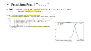
Ꚛ Let’s use the cross_val_score() function to evaluate your SGDClassifier
model using K-fold crossvalidation, with three folds.
Ꚛ Remember that K-fold cross-validation means splitting the training set
into K-folds (in this case, three), then making predictions and evaluating
them on each fold using a model trained on the remaining folds
▪ from sklearn.model_selection import cross_val_score
▪ cross_val_score(sgd_clf, X_train, y_train_5, cv=3, scoring="accuracy")
▪ Out[24]: array([0.94555, 0.9012 , 0.9625 ])
Ꚛ Wow! Around 95% accuracy (ratio of correct predictions) on all cross-
validation folds? This looks amazing, doesn’t it?](https://image.slidesharecdn.com/hwknmajmrfk2q6n51lrk-signature-8de60c98476d684bd50cee58acbea27ff40abfe38959d4d51c6e1d5d4629c2e1-poli-200307202646/85/Lecture-12-binary-classifier-confusion-matrix-11-320.jpg)


Lecture 12 binary classifier confusion matrix
- 1. ClassificationDr. Mostafa A. Elhosseini
- 2. Revise Ꚛ Regression task Ꚛ Predicting Housing values using ▪ Linear Regression ▪ How to fix underfitting ▪ Decision Trees. ▪ Random Forest Ꚛ Cross-validation Ꚛ Fine-tune your model ▪ Grid Search ▪ Randomized Search ▪ Ensemble Methods Ꚛ Hyberparameter
- 3. Agenda Ꚛ Handwritten digits dataset MINST
- 4. MINST Ꚛ Set of 70,000 small images of digits handwritten by high school students and employees of the US Census Bureau Ꚛ Each image is labeled with the digit it represents Ꚛ It is often called the “Hello World” of Machine Learning Ꚛ Each image has 28×28 pixels (784 features ) Ꚛ Each feature simply represents one pixel’s intensity, from 0 (white) to 255 (black)
- 5. MINST Ꚛ Datasets loaded by Scikit- Learn generally have a similar dictionary structure including: ▪ A DESCR key describing the dataset ▪ A data key containing an array with one row per instance and one column per feature ▪ A target key containing an array with the labels
- 6. Peek at one digit from the dataset
- 7. ▪ To feel complexity of the classification task
- 8. MINST Training & Testing set Ꚛ You should always create a test set and set it aside before inspecting the data closely. Ꚛ The MNIST dataset is actually already split into a training set (the first 60,000 images) and a test set (the last 10,000 images): Ꚛ Shuffle the training set; this will guarantee that… ▪ All cross-validation folds will be similar (you don’t want one fold to be missing some digits). ▪ Moreover, some learning algorithms are sensitive to the order of the training instances, and they perform poorly if they get many similar instances in a row. Shuffling the dataset ensures that this won’t happen:
- 9. Training Binary Classifier Ꚛ Let’s simplify the problem for now and only try to identify one digit — for example, the number 5. Ꚛ This “5-detector” will be an example of a binary classifier, capable of distinguishing between just two classes, 5 and not-5. Let’s create the target vectors for this classification task: ▪ y_train_5 = (y_train == 5) # True for all 5s, False for all other digits. ▪ y_test_5 = (y_test == 5) Ꚛ Okay, now let’s pick a classifier and train it. A good place to start is with a Stochastic Gradient Descent (SGD) classifier, using Scikit- Learn’s SGDClassifier class
- 10. Stochastic Gradient Descent Classifier Ꚛ This classifier has the advantage of being capable of handling very large datasets efficiently. Ꚛ This is in part because SGD deals with training instances independently, one at a time (which also makes SGD well suited for online learning), as we will see later. ▪ from sklearn.linear_model import SGDClassifier ▪ sgd_clf = SGDClassifier(random_state=42) ▪ sgd_clf.fit(X_train, y_train_5) Ꚛ The SGDClassifier relies on randomness during training (hence the name “stochastic”). Ꚛ If you want reproducible results, you should set the random_state parameter. Ꚛ The classifier guesses that this image represents a 5 (True)
- 11. Performance Measures Ꚛ Evaluating a classifier is often significantly trickier than evaluating a regressor Ꚛ Let’s use the cross_val_score() function to evaluate your SGDClassifier model using K-fold crossvalidation, with three folds. Ꚛ Remember that K-fold cross-validation means splitting the training set into K-folds (in this case, three), then making predictions and evaluating them on each fold using a model trained on the remaining folds ▪ from sklearn.model_selection import cross_val_score ▪ cross_val_score(sgd_clf, X_train, y_train_5, cv=3, scoring="accuracy") ▪ Out[24]: array([0.94555, 0.9012 , 0.9625 ]) Ꚛ Wow! Around 95% accuracy (ratio of correct predictions) on all cross- validation folds? This looks amazing, doesn’t it?
- 12. Dumb classifier ▪ Well, before you get too excited, let’s look at a very dumb classifier that just classifies every single image in the “not-5” class
- 13. Dumb classifier Ꚛ It has over 90% accuracy! This is simply because only about 10% of the images are 5s, so if you always guess that an image is not a 5, you will be right about 90% of the time. Ꚛ This demonstrates why accuracy is generally not the preferred performance measure for classifiers, especially when you are dealing with skewed datasets (i.e., when some classes are much more frequent than others)
- 14. Confusion Matrix Ꚛ A much better way to evaluate the performance of a classifier is to look at the confusion matrix. Ꚛ The general idea is to count the number of times instances of class A are classified as class B ▪ For example, to know the number of times the classifier confused images of 5s with 3s, you would look in the 5th row and 3rd column of the confusion matrix Ꚛ To compute the confusion matrix, you first need to have a set of predictions, so they can be compared to the actual targets. Ꚛ You could make predictions on the test set, but let’s keep it untouched for now (remember that you want to use the test set only at the very end of your project, once you have a classifier that you are ready to launch). ▪ Instead, you can use the cross_val_predict() function:
- 15. Confusion Matrix ▪ from sklearn.model_selection import cross_val_predict ▪ y_train_pred = cross_val_predict(sgd_clf, X_train, y_train_5, cv=3)
- 16. Confusion Matrix Ꚛ Each row in a confusion matrix represents an actual class, while each column represents a predicted class. Ꚛ The first row of this matrix considers non-5 images (the negative class): 53,272 of them were correctly classified as non-5s (they are called true negatives TN), ▪ while the remaining 1,307 were wrongly classified as 5s (false positives FP). Ꚛ The second row considers the images of 5s (the positive class): 1,077 were wrongly classified as non-5s (false negatives FN), while the remaining 4,344 were correctly classified as 5s (true positives TP). Ꚛ A perfect classifier would have only true positives and true negatives, so its confusion matrix would have nonzero values only on its main diagonal (top left to bottom right)
- 17. ▪ 𝑃𝑟𝑒𝑐𝑖𝑠𝑖𝑜𝑛 = 𝑇𝑃 𝑇𝑃+𝐹𝑃 ▪ Accuracy of the positive predictions ▪ 𝑅𝑒𝑐𝑎𝑙𝑙 = 𝑇𝑃 𝑇𝑃+𝐹𝑁 ▪ Sensitivity = True Positive Rate TPR
- 18. Confusion Matrix ▪ Now your 5-detector does not look as shiny as it did when you looked at its accuracy. ▪ When it claims an image represents a 5, it is correct only 77% of the time. Moreover, it only detects 79% of the 5s
- 19. 𝐹1Score • It is often convenient to combine precision and recall into a single metric called the 𝐹1 score, in particular if you need a simple way to compare two classifiers. • The 𝐹1 score is the harmonic mean of precision and recall • Whereas the regular mean treats all values equally, the harmonic mean gives much more weight to low values. As a result, the classifier will only get a high 𝐹1 score if both recall and precision are high
- 20. Which is more important – Precision / Recall? Ꚛ The 𝐹1 score favors classifiers that have similar precision and recall. This is not always what you want: in some contexts you mostly care about precision, and in other contexts you really care about recall. Ꚛ For example, if you trained a classifier to detect videos that are safe for kids, you would probably prefer a classifier that rejects many good videos (low recall) but keeps only safe ones (high precision), rather than a classifier that has a much higher recall but lets a few really bad videos show up in your product Ꚛ On the other hand, suppose you train a classifier to detect shoplifters on surveillance images: it is probably fine if your classifier has only 30% precision as long as it has 99% recall (sure, the security guards will get a few false alerts, but almost all shoplifters will get caught).
- 21. Precision/Recall Tradeoff Ꚛ To understand this tradeoff, let’s look at how the SGDClassifier makes its classification decisions. ▪ For each instance, it computes a score based on a decision function, and if that score is greater than a threshold, it assigns the instance to the positive class, or else it assigns it to the negative class Ꚛ Figure below shows a few digits positioned from the lowest score on the left to the highest score on the right. ▪ Suppose the decision threshold is positioned at the central arrow (between the two 5s): you will find 4 true positives (actual 5s) on the right of that threshold, and one false positive (actually a 6). ▪ Therefore, with that threshold, the precision is 80% (4 out of 5). But out of 6 actual 5s, the classifier only detects 4, so the recall is 67% (4 out of 6). Ꚛ Now if you raise the threshold (move it to the arrow on the right), the false positive (the 6) becomes a true negative, thereby increasing precision (up to 100% in this case), but one true positive becomes a false negative, decreasing recall down to 50%. Conversely, lowering the threshold increases recall and reduces precision
- 23. Precision/Recall Tradeoff Ꚛ Scikit-Learn does not let you set the threshold directly, but it does give you access to the decision scores that it uses to make predictions. Ꚛ Instead of calling the classifier’s predict() method, you can call its decision_function() method, which returns a score for each instance, and then make predictions based on those scores using any threshold you want:
- 24. Precision/Recall Tradeoff Ꚛ This confirms that raising the threshold decreases recall. The image actually represents a 5, and the classifier detects it when the threshold is 0, but it misses it when the threshold is increased to 200,000. Ꚛ So how can you decide which threshold to use? For this you will first need to get the scores of all instances in the training set using the cross_val_predict() function again, but this time specifying that you want it to return decision scores instead of predictions:
- 26. Precision/Recall Tradeoff Ꚛ You may wonder why the precision curve is bumpier than the recall curve in Figure 3-4. The reason is that precision may sometimes go down when you raise the threshold (although in general it will go up). Ꚛ To understand why, look back at Figure and notice what happens when you start from the central threshold and move it just one digit to the right: precision goes from 4/5 (80%) down to 3/4 (75%). Ꚛ On the other hand, recall can only go down when the threshold is increased, which explains why its curve looks smooth
- 27. Precision/Recall Tradeoff Ꚛ Now you can simply select the threshold value that gives you the best precision/recall tradeoff for your task. Ꚛ Another way to select a good precision/recall tradeoff is to plot precision directly against recall You can see that precision really starts to fall sharply around 80% recall. You will probably want to select a precision/recall tradeoff just before that drop — for example, at around 60% recall. But of course the choice depends on your project
- 28. Precision/Recall Tradeoff Ꚛ So let’s suppose you decide to aim for 90% precision. Ꚛ You look up the first plot (zooming in a bit) and find that you need to use a threshold of about 230,000. To make predictions (on the training set for now), instead of calling the classifier’s predict() method, you can just run this code:
- 29. Precision/Recall Tradeoff Ꚛ Great, you have a 90% precision classifier (or close enough)! As you can see, it is fairly easy to create a classifier with virtually any precision you want: just set a high enough threshold, and you’re done. Ꚛ Hmm, not so fast. A high-precision classifier is not very useful if its recall is too low! Ꚛ If someone says “let’s reach 99% precision,” you should ask, “at what recall?”
- 30. The ROC Curve Ꚛ The Receiver Operating Characteristic (ROC) curve is another common tool used with binary classifiers. Ꚛ ROC curve plots the true positive rate (another name for recall) against the false positive rate FPR Ꚛ The FPR is the ratio of negative instances that are incorrectly classified as positive. ▪ It is equal to one minus the true negative rate, which is the ratio of negative instances that are correctly classified as negative. Ꚛ The TNR is also called specificity. Ꚛ Hence the ROC curve plots sensitivity (recall) versus 1 – specificity.
- 31. ▪ The ROC Curve ▪ Once again there is a tradeoff: the higher the recall (TPR), the more false positives (FPR) the classifier produces. ▪ The dotted line represents the ROC curve of a purely random classifier ▪ A good classifier stays as far away from that line as possible (toward the top-left corner).
- 32. ▪ The ROC Curve Ꚛ One way to compare classifiers is to measure the Area Under the Curve (AUC). Ꚛ A perfect classifier will have a ROC AUC equal to 1, whereas a purely random classifier will have a ROC AUC equal to 0.5. Ꚛ Scikit-Learn provides a function to compute the ROC AUC: ▪ from sklearn.metrics import roc_auc_score ▪ roc_auc_score(y_train_5, y_scores) Ꚛ As a rule of thumb, you should prefer the PR curve whenever the positive class is rare or when you care more about the false positives than the false negatives, and the ROC curve otherwise
- 33. ▪ The ROC Curve Ꚛ Let’s train a RandomForestClassifier and compare its ROC curve and ROC AUC score to the SGDClassifier. Ꚛ First, you need to get scores for each instance in the training set. ▪ But due to the way it works, the RandomForestClassifier class does not have a decision_function() method. Ꚛ Instead it has a predict_proba() method. Scikit-Learn classifiers generally have one or the other. Ꚛ The predict_proba() method returns an array containing a row per instance and a column per class, each containing the probability that the given instance belongs to the given class (e.g., 70% chance that the image represents a 5):
- 34. ▪ The ROC Curve ▪ But to plot a ROC curve, you need scores, not probabilities. A simple solution is to use the positive class’s probability as the score:
- 35. ▪ The ROC Curve Ꚛ The RandomForestClassifier’s ROC curve looks much better than the SGDClassifier’s: it comes much closer to the top-left corner. Ꚛ As a result, its ROC AUC score is also significantly better: