SlideShare a Scribd company logo
UNIT 3
Linear Programming - Introduction
Dr. Kailash Chaudhary
Ph.D. (Mechanical Design), M.E. (P & I), B.E. (Mechanical Engg)
Assistant Professor
Department of Mechanical Engineering
MBM Engineering College
ME 342 A
System Design and Analysis
Lecture Contents
Introduction to optimization
Modelling and Solving simple problems
Modelling combinatorial problems.
Duality or Assessing the quality of a solution.
Motivation
Why linear programming is a very important topic?
• A lot of problems can be formulated as linear
programmes
• There exist efficient methods to solve them
• or at least give good approximations.
• Solve difficult problems: e.g. original example given
by the inventor of the theory, Dantzig. Best
assignment of 70 people to 70 tasks.
What is a linear programme?
• Optimization problem consisting in
• Maximizing (or minimizing) a linear objective
function
• of n decision variables
• subject to a set of constraints expressed by
linear equations or inequalities.
• Terminology due to George B. Dantzig, inventor of
the Simplex Algorithm (1947)
Terminology
max 350x1 + 300x2
subject to
x1 + x2 ≤200
9x1 + 6x2 ≤1566
12x1 + 16x2 ≤2880
x1, x2 ≥0
x1,x2 : Decision variables
Objective function
Constraints
Terminology
max 350x1 + 300x2
subject to
x1 + x2 ≤200
9x1 + 6x2 ≤1566
12x1 + 16x2 ≤2880
x1, x2 ≥0
x1,x2 : Decision variables
Objective function
Constraints
In linear programme: objective function + constraints
are all linear
Typically (not always): variables are non-negative
If variables are integer: system called Integer
Programme (IP)
Terminology
xj ≥ 0 for all 1 ≤j ≤n.
• the problem is a maximization;
• all constraints are inequalities (and not equations);
• all variables are non-negative.
Linear programmes can be written under the standard form:
∑n
j=1 cjxj
Maximize
Subject to: ∑n
j=1 aijxj ≤ bi for all 1 ≤i ≤m (1)
Example 1: a resource allocation
problem
A company produces copper cable of 5 and 10 mm of diameter on a
single production line with the following constraints:
• The available copper allows to produces 21000 meters of cable of
5 mm diameter per week.
• A meter of 10 mm diameter copper consumes 4 times more
copper than a meter of 5 mm diameter copper.
Due to demand, the weekly production of 5 mm cable is limited to
15000 meters and the production of 10 mm cable should not exceed
40% of the total production. Cable are respectively sold 50 and 200
euros the meter.
What should the company produce in order to maximize its weekly
revenue?
Define two decision variables:
• x1: the number of thousands of meters of 5 mm cables produced
every week
• x2: the number of thousands meters of 10 mm cables produced
every week
The revenue associated to a production (x1,x2) is
z = 50x1 + 200x2.
The capacity of production cannot be exceeded
x1 + 4x2 ≤21.
The demand constraints have to be satisfied
2
4
10
x ≤ ( 1 2
x + x )
x1 ≤15
Negative quantities cannot be produced
x1 ≥0,x2 ≥0.
The model: To maximize the sell revenue, determine the solutions of
the following linear programme x1 and x2:
max z = 50x1 + 200x2
subject to
x1 + 4x2 ≤21
−4x1 + 6x2 ≤0
x1 ≤15
x1,x2 ≥0
Example 2: Scheduling
• m = 3 machines
• n = 8 tasks
• Each task lasts x units of
time
Objective: affect the tasks to the machines in order to minimize the
duration
• Here, the 8 tasks are finished after 7 units of times on 3
machines.
• m = 3 machines
• n = 8 tasks
• Each task lasts x units of
time
Objective: affect the tasks to the machines in order to minimize the
duration
• Now, the 8 tasks are accomplished after 6.5 units of time
Graphical Method
• The constraints of a linear programme define a
zone of solutions.
• The best point of the zone corresponds to the
optimal solution.
• For problem with 2 variables, easy to draw the
zone of solutions and to find the optimal solution
graphically.
Graphical Method
Example:
max 350x1 +300x2
subject to
x1 + x2 ≤200
9x1 + 6x2 ≤1566
12x1 + 16x2 ≤2880
x1, x2 ≥0
Lecture - Linear Programming.pdf
Computation of optimal solution
The optimal solution is at the intersection of the constraints:
x1 + x2 = 200 (2)
9x1 + 6x2 = 1566 (3)
We get:
x1 = 122
x2 = 78
Objective = 66100.
Optimal Solutions:
Different Cases
Three different possible cases:
• a single optimal solution,
• an infinite number of optimal solutions, or
• no optimal solutions.
• If an optimal solution exists, there is always a
corner point optimal solution!
Solving Linear Programmes
• The constraints of an LP give rise to a geometrical shape:
a polyhedron
• If we can determine all the corner points of the polyhedron, then
we calculate the objective function at these points and take the
best one as our optimal solution.
• The Simplex Method intelligently moves from corner to corner
until it can prove that it has found the optimal solution.
Solving Linear Programmes
• Geometric method impossible in higher dimensions
• Algebraical methods:
• Simplex method (George B. Dantzig 1949):
skim through the feasible solution polytope.
Similar to a "Gaussian elimination".
Very good in practice, but can take an
exponential time.
But Integer Programming
(IP) is different!
• Feasible region: a set of
discrete points.
• Corner point solution not
assured.
• No "efficient" way to solve
an IP.
• Solving it as an LP provides
a relaxation and a bound on
the solution.
Linear programming example 1
A company is involved in the production of two items (X and Y). The resources
need to produce X and Y are twofold, namely machine time for automatic
processing and craftsman time for hand finishing. The table below gives the
number of minutes required for each item:
Machine time Craftsman time
Item X 13 20
Y 19 29
The company has 40 hours of machine time available in the next working week
but only 35 hours of craftsman time. Machine time is costed at rupees10 per
hour worked and craftsman time is costed at rupees 2 per hour worked. Both
machine and craftsman idle times incur no costs. The revenue received for each
item produced (all production is sold) is rupees 20 for X and rupees 30 for Y.
The company has a specific contract to produce 10 items of X per week for a
particular customer.
 Formulate the problem of deciding how much to produce per week as a
linear program.
 Solve this linear program graphically.
Solution
Let
 x be the number of items of X
 y be the number of items of Y
then the LP is:
maximise
 20x + 30y - 10(machine time worked) - 2(craftsman time worked)
subject to:
 13x + 19y <= 40(60) machine time
 20x + 29y <= 35(60) craftsman time
 x >= 10 contract
 x,y >= 0
so that the objective function becomes
maximise
 20x + 30y - 10(13x + 19y)/60 - 2(20x + 29y)/60
i.e. maximise
 17.1667x + 25.8667y
subject to:
 13x + 19y <= 2400
 20x + 29y <= 2100
 x >= 10
 x,y >= 0
It is plain from the diagram below that the maximum occurs at the intersection
of x=10 and 20x + 29y <= 2100
Solving simultaneously, rather than by reading values off the graph, we have
that x=10 and y=65.52 with the value of the objective function being rupees
1866.5
Linear programming example 2
A company manufactures two products (A and B) and the profit per unit sold is
rupees 3 and rupees 5 respectively. Each product has to be assembled on a
particular machine, each unit of product A taking 12 minutes of assembly time
and each unit of product B 25 minutes of assembly time. The company
estimates that the machine used for assembly has an effective working week of
only 30 hours (due to maintenance/breakdown).
Technological constraints mean that for every five units of product A produced
at least two units of product B must be produced.
 Formulate the problem of how much of each product to produce as a
linear program.
 Solve this linear program graphically.
 The company has been offered the chance to hire an extra machine,
thereby doubling the effective assembly time available. What is
the maximum amount you would be prepared to pay (per week) for the
hire of this machine and why?
Solution
Let
xA = number of units of A produced
xB = number of units of B produced
then the constraints are:
12xA + 25xB <= 30(60) (assembly time)
xB >= 2(xA/5)
i.e. xB - 0.4xA >= 0
i.e. 5xB >= 2xA (technological)
where xA, xB >= 0
and the objective is
maximise 3xA + 5xB
It is plain from the diagram below that the maximum occurs at the intersection
of 12xA + 25xB = 1800 and xB - 0.4xA = 0
Solving simultaneously, rather than by reading values off the graph, we have
that:
xA= (1800/22) = 81.8
xB= 0.4xA = 32.7
with the value of the objective function being rupees 408.9
Doubling the assembly time available means that the assembly time constraint
(currently 12xA + 25xB <= 1800) becomes 12xA + 25xB <= 2(1800) This new
constraint will be parallel to the existing assembly time constraint so that the
new optimal solution will lie at the intersection of 12xA + 25xB = 3600 and xB -
0.4xA = 0
i.e. at xA = (3600/22) = 163.6
xB= 0.4xA = 65.4
with the value of the objective function being rupees 817.8
Hence we have made an additional profit of rupees (817.8-408.9) = rupees
408.9 and this is the maximum amount we would be prepared to pay for the hire
of the machine for doubling the assembly time.
This is because if we pay more than this amount then we will reduce our
maximum profit below the rupees 408.9 we would have made without the
new machine.
Linear programming example 3
Solve
minimise
4a + 5b + 6c
subject to
a + b >= 11
a - b <= 5
c - a - b = 0
7a >= 35 - 12b
a >= 0 b >= 0 c >= 0
Solution
To solve this LP we use the equation c-a-b=0 to put c=a+b (>= 0 as a >= 0 and
b >= 0) and so the LP is reduced to
minimise
4a + 5b + 6(a + b) = 10a + 11b
subject to
a + b >= 11
a - b <= 5
7a + 12b >= 35
a >= 0 b >= 0
From the diagram below the minimum occurs at the intersection of a - b = 5 and
a + b = 11
i.e. a = 8 and b = 3 with c (= a + b) = 11 and the value of the objective function
10a + 11b = 80 + 33 = 113.
Linear programming example 4
Solve the following linear program:
maximise 5x1 + 6x2
subject to
x1 + x2 <= 10
x1 - x2 >= 3
5x1 + 4x2 <= 35
x1 >= 0
x2 >= 0
Solution
It is plain from the diagram below that the maximum occurs at the intersection
of
5x1 + 4x2 = 35 and
x1 - x2 = 3
Solving simultaneously, rather than by reading values off the graph, we have
that
5(3 + x2) + 4x2 = 35
i.e. 15 + 9x2 = 35
i.e. x2 = (20/9) = 2.222 and
x1 = 3 + x2 = (47/9) = 5.222
The maximum value is 5(47/9) + 6(20/9) = (355/9) = 39.444
Linear programming example 5
A carpenter makes tables and chairs. Each table can be sold for a profit of
rupees 30 and each chair for a profit of rupees 10. The carpenter can afford to
spend up to 40 hours per week working and takes six hours to make a table and
three hours to make a chair. Customer demand requires that he makes at least
three times as many chairs as tables. Tables take up four times as much storage
space as chairs and there is room for at most four tables each week.
Formulate this problem as a linear programming problem and solve it
graphically.
Solution
Variables
Let
xT = number of tables made per week
xC = number of chairs made per week
Constraints
 total work time
6xT + 3xC <= 40
 customer demand
xC >= 3xT
 storage space
(xC/4) + xT <= 4
 all variables >= 0
Objective
maximise 30xT + 10xC
The graphical representation of the problem is given below and from that we
have that the solution lies at the intersection of
(xC/4) + xT = 4 and 6xT + 3xC = 40
Solving these two equations simultaneously we get xC = 10.667, xT = 1.333 and
the corresponding profit = rupees 146.667
Additional problems for exercise: Chapter 2 of Operation
Research book by H A Taha
Ad

Recommended

Ap for b.tech. (mechanical) Assignment Problem
Prashant Khandelwal
 
Assignment problem
Assignment problem
Harshil Vakani
 
Assignment Problem
Assignment Problem
Nakul Bhardwaj
 
Stepping Stone Method
Himanshi Gupta
 
Transportation and Assignment
Lokesh Payasi
 
Assignment Chapter - Q & A Compilation by Niraj Thapa
CA Niraj Thapa
 
Assignment Poblems
Assignment Poblems
vkabre
 
Nature and scope of managerial economics
Harinadh Karimikonda
 
Linear programing
Linear programing
anam katmale
 
Scope of Managerial Economics
Rajat Busheheri
 
Simplex method concept,
Dronak Sahu
 
Transportation problems
VishalHotchandani2
 
Assignment Problem
Assignment Problem
JIMS Rohini Sector 5
 
Assignment oprations research luv
Ashok Sharma
 
Mba i qt unit-1.3_linear programming in om
Rai University
 
Importance of Operation Research in Decision Making – MIT School of Distance ...
MIT School
 
Vogel’s Approximation Method (VAM)
dkpawar
 
Formulation Lpp
Formulation Lpp
Sachin MK
 
Linear Programming
Linear Programming
Pulchowk Campus
 
Linear programing
Linear programing
Aniruddh Tiwari
 
Replacement Theory Models in Operations Research by Dr. Rajesh Timane
Rajesh Timane, PhD
 
Solving Degenaracy in Transportation Problem
mkmanik
 
Linear programming Cost Minimization
Khushbu :-)
 
Unit.3. duality and sensetivity analisis
DagnaygebawGoshme
 
3. linear programming senstivity analysis
Hakeem-Ur- Rehman
 
Project Management- Unit V
Lamay Sabir
 
Simplex Method
Simplex Method
Sachin MK
 
Decision Theory Lecture Notes.pdf
Dr. Tushar J Bhatt
 
introduction to Operation Research
amanyosama12
 
Management Science
Management Science
Renzhie Katigbak
 

More Related Content

What's hot (20)

Linear programing
Linear programing
anam katmale
 
Scope of Managerial Economics
Rajat Busheheri
 
Simplex method concept,
Dronak Sahu
 
Transportation problems
VishalHotchandani2
 
Assignment Problem
Assignment Problem
JIMS Rohini Sector 5
 
Assignment oprations research luv
Ashok Sharma
 
Mba i qt unit-1.3_linear programming in om
Rai University
 
Importance of Operation Research in Decision Making – MIT School of Distance ...
MIT School
 
Vogel’s Approximation Method (VAM)
dkpawar
 
Formulation Lpp
Formulation Lpp
Sachin MK
 
Linear Programming
Linear Programming
Pulchowk Campus
 
Linear programing
Linear programing
Aniruddh Tiwari
 
Replacement Theory Models in Operations Research by Dr. Rajesh Timane
Rajesh Timane, PhD
 
Solving Degenaracy in Transportation Problem
mkmanik
 
Linear programming Cost Minimization
Khushbu :-)
 
Unit.3. duality and sensetivity analisis
DagnaygebawGoshme
 
3. linear programming senstivity analysis
Hakeem-Ur- Rehman
 
Project Management- Unit V
Lamay Sabir
 
Simplex Method
Simplex Method
Sachin MK
 
Decision Theory Lecture Notes.pdf
Dr. Tushar J Bhatt
 
Scope of Managerial Economics
Rajat Busheheri
 
Simplex method concept,
Dronak Sahu
 
Assignment oprations research luv
Ashok Sharma
 
Mba i qt unit-1.3_linear programming in om
Rai University
 
Importance of Operation Research in Decision Making – MIT School of Distance ...
MIT School
 
Vogel’s Approximation Method (VAM)
dkpawar
 
Formulation Lpp
Formulation Lpp
Sachin MK
 
Replacement Theory Models in Operations Research by Dr. Rajesh Timane
Rajesh Timane, PhD
 
Solving Degenaracy in Transportation Problem
mkmanik
 
Linear programming Cost Minimization
Khushbu :-)
 
Unit.3. duality and sensetivity analisis
DagnaygebawGoshme
 
3. linear programming senstivity analysis
Hakeem-Ur- Rehman
 
Project Management- Unit V
Lamay Sabir
 
Simplex Method
Simplex Method
Sachin MK
 
Decision Theory Lecture Notes.pdf
Dr. Tushar J Bhatt
 

Similar to Lecture - Linear Programming.pdf (20)

introduction to Operation Research
amanyosama12
 
Management Science
Management Science
Renzhie Katigbak
 
Chapter 2.Linear Programming.pdf
Tsegay Berhe
 
Operation research ppt chapter two mitku
mitku assefa
 
Operation research chapter two linear programming
selome993
 
Introduction to Linear programing.ORpptx
aishaashraf31
 
Linear Programing.pptx
AdnanHaleem
 
Graphical Solution in LPP along with graphs and formula
SUDIPTAADHIKARY15
 
Linear programming
Linear programming
Tarun Gehlot
 
Linear programming graphical method
Dr. Abdulfatah Salem
 
Mathematics For Management CHAPTER THREE PART I.PPT
AYNETUTEREFE1
 
V -linear_programming
Yashwant Raj Verma
 
Linear Programming 1
irsa javed
 
chapter 2 revised.pptx
DejeneDay
 
Quantitativetechniqueformanagerialdecisionlinearprogramming 090725035417-phpa...
kongara
 
chapter 2 revised.pptx
DejeneDay
 
Ees 300
Ees 300
AgwonaMAllan
 
Linear Programming Module- A Conceptual Framework
Sasquatch S
 
Linear Models for Engineering applications
KalinduDilanjan
 
Linear programming.pptx
Prabin Pandit
 
introduction to Operation Research
amanyosama12
 
Chapter 2.Linear Programming.pdf
Tsegay Berhe
 
Operation research ppt chapter two mitku
mitku assefa
 
Operation research chapter two linear programming
selome993
 
Introduction to Linear programing.ORpptx
aishaashraf31
 
Linear Programing.pptx
AdnanHaleem
 
Graphical Solution in LPP along with graphs and formula
SUDIPTAADHIKARY15
 
Linear programming
Linear programming
Tarun Gehlot
 
Linear programming graphical method
Dr. Abdulfatah Salem
 
Mathematics For Management CHAPTER THREE PART I.PPT
AYNETUTEREFE1
 
Linear Programming 1
irsa javed
 
chapter 2 revised.pptx
DejeneDay
 
Quantitativetechniqueformanagerialdecisionlinearprogramming 090725035417-phpa...
kongara
 
chapter 2 revised.pptx
DejeneDay
 
Linear Programming Module- A Conceptual Framework
Sasquatch S
 
Linear Models for Engineering applications
KalinduDilanjan
 
Linear programming.pptx
Prabin Pandit
 
Ad

Recently uploaded (20)

International Journal of Advanced Information Technology (IJAIT)
ijait
 
AI_Presentation (1). Artificial intelligence
RoselynKaur8thD34
 
Learning – Types of Machine Learning – Supervised Learning – Unsupervised UNI...
23Q95A6706
 
Introduction to Python Programming Language
merlinjohnsy
 
最新版美国圣莫尼卡学院毕业证(SMC毕业证书)原版定制
Taqyea
 
Abraham Silberschatz-Operating System Concepts (9th,2012.12).pdf
Shabista Imam
 
Decoding Kotlin - Your Guide to Solving the Mysterious in Kotlin - Devoxx PL ...
João Esperancinha
 
IntroSlides-June-GDG-Cloud-Munich community [email protected]
Luiz Carneiro
 
Complete University of Calculus :: 2nd edition
Shabista Imam
 
ElysiumPro Company Profile 2025-2026.pdf
info751436
 
System design handwritten notes guidance
Shabista Imam
 
Structured Programming with C++ :: Kjell Backman
Shabista Imam
 
IPL_Logic_Flow.pdf Mainframe IPLMainframe IPL
KhadijaKhadijaAouadi
 
Microwatt: Open Tiny Core, Big Possibilities
IBM
 
Industry 4.o the fourth revolutionWeek-2.pptx
KNaveenKumarECE
 
Stay Safe Women Security Android App Project Report.pdf
Kamal Acharya
 
nnnnnnnnnnnn7777777777777777777777777777777.pptx
gayathri venkataramani
 
Tally.ERP 9 at a Glance.book - Tally Solutions .pdf
Shabista Imam
 
60 Years and Beyond eBook 1234567891.pdf
waseemalazzeh
 
Mechanical Vibration_MIC 202_iit roorkee.pdf
isahiliitr
 
International Journal of Advanced Information Technology (IJAIT)
ijait
 
AI_Presentation (1). Artificial intelligence
RoselynKaur8thD34
 
Learning – Types of Machine Learning – Supervised Learning – Unsupervised UNI...
23Q95A6706
 
Introduction to Python Programming Language
merlinjohnsy
 
最新版美国圣莫尼卡学院毕业证(SMC毕业证书)原版定制
Taqyea
 
Abraham Silberschatz-Operating System Concepts (9th,2012.12).pdf
Shabista Imam
 
Decoding Kotlin - Your Guide to Solving the Mysterious in Kotlin - Devoxx PL ...
João Esperancinha
 
Complete University of Calculus :: 2nd edition
Shabista Imam
 
ElysiumPro Company Profile 2025-2026.pdf
info751436
 
System design handwritten notes guidance
Shabista Imam
 
Structured Programming with C++ :: Kjell Backman
Shabista Imam
 
IPL_Logic_Flow.pdf Mainframe IPLMainframe IPL
KhadijaKhadijaAouadi
 
Microwatt: Open Tiny Core, Big Possibilities
IBM
 
Industry 4.o the fourth revolutionWeek-2.pptx
KNaveenKumarECE
 
Stay Safe Women Security Android App Project Report.pdf
Kamal Acharya
 
nnnnnnnnnnnn7777777777777777777777777777777.pptx
gayathri venkataramani
 
Tally.ERP 9 at a Glance.book - Tally Solutions .pdf
Shabista Imam
 
60 Years and Beyond eBook 1234567891.pdf
waseemalazzeh
 
Mechanical Vibration_MIC 202_iit roorkee.pdf
isahiliitr
 
Ad

Lecture - Linear Programming.pdf

  • 1. UNIT 3 Linear Programming - Introduction Dr. Kailash Chaudhary Ph.D. (Mechanical Design), M.E. (P & I), B.E. (Mechanical Engg) Assistant Professor Department of Mechanical Engineering MBM Engineering College ME 342 A System Design and Analysis
  • 2. Lecture Contents Introduction to optimization Modelling and Solving simple problems Modelling combinatorial problems. Duality or Assessing the quality of a solution.
  • 3. Motivation Why linear programming is a very important topic? • A lot of problems can be formulated as linear programmes • There exist efficient methods to solve them • or at least give good approximations. • Solve difficult problems: e.g. original example given by the inventor of the theory, Dantzig. Best assignment of 70 people to 70 tasks.
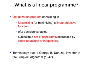
  • 4. What is a linear programme? • Optimization problem consisting in • Maximizing (or minimizing) a linear objective function • of n decision variables • subject to a set of constraints expressed by linear equations or inequalities. • Terminology due to George B. Dantzig, inventor of the Simplex Algorithm (1947)
  • 5. Terminology max 350x1 + 300x2 subject to x1 + x2 ≤200 9x1 + 6x2 ≤1566 12x1 + 16x2 ≤2880 x1, x2 ≥0 x1,x2 : Decision variables Objective function Constraints
  • 6. Terminology max 350x1 + 300x2 subject to x1 + x2 ≤200 9x1 + 6x2 ≤1566 12x1 + 16x2 ≤2880 x1, x2 ≥0 x1,x2 : Decision variables Objective function Constraints In linear programme: objective function + constraints are all linear Typically (not always): variables are non-negative If variables are integer: system called Integer Programme (IP)
  • 7. Terminology xj ≥ 0 for all 1 ≤j ≤n. • the problem is a maximization; • all constraints are inequalities (and not equations); • all variables are non-negative. Linear programmes can be written under the standard form: ∑n j=1 cjxj Maximize Subject to: ∑n j=1 aijxj ≤ bi for all 1 ≤i ≤m (1)
  • 8. Example 1: a resource allocation problem A company produces copper cable of 5 and 10 mm of diameter on a single production line with the following constraints: • The available copper allows to produces 21000 meters of cable of 5 mm diameter per week. • A meter of 10 mm diameter copper consumes 4 times more copper than a meter of 5 mm diameter copper. Due to demand, the weekly production of 5 mm cable is limited to 15000 meters and the production of 10 mm cable should not exceed 40% of the total production. Cable are respectively sold 50 and 200 euros the meter. What should the company produce in order to maximize its weekly revenue?
  • 9. Define two decision variables: • x1: the number of thousands of meters of 5 mm cables produced every week • x2: the number of thousands meters of 10 mm cables produced every week The revenue associated to a production (x1,x2) is z = 50x1 + 200x2. The capacity of production cannot be exceeded x1 + 4x2 ≤21.
  • 10. The demand constraints have to be satisfied 2 4 10 x ≤ ( 1 2 x + x ) x1 ≤15 Negative quantities cannot be produced x1 ≥0,x2 ≥0.
  • 11. The model: To maximize the sell revenue, determine the solutions of the following linear programme x1 and x2: max z = 50x1 + 200x2 subject to x1 + 4x2 ≤21 −4x1 + 6x2 ≤0 x1 ≤15 x1,x2 ≥0
  • 12. Example 2: Scheduling • m = 3 machines • n = 8 tasks • Each task lasts x units of time Objective: affect the tasks to the machines in order to minimize the duration • Here, the 8 tasks are finished after 7 units of times on 3 machines.
  • 13. • m = 3 machines • n = 8 tasks • Each task lasts x units of time Objective: affect the tasks to the machines in order to minimize the duration • Now, the 8 tasks are accomplished after 6.5 units of time
  • 14. Graphical Method • The constraints of a linear programme define a zone of solutions. • The best point of the zone corresponds to the optimal solution. • For problem with 2 variables, easy to draw the zone of solutions and to find the optimal solution graphically.
  • 15. Graphical Method Example: max 350x1 +300x2 subject to x1 + x2 ≤200 9x1 + 6x2 ≤1566 12x1 + 16x2 ≤2880 x1, x2 ≥0
  • 22. Computation of optimal solution The optimal solution is at the intersection of the constraints: x1 + x2 = 200 (2) 9x1 + 6x2 = 1566 (3) We get: x1 = 122 x2 = 78 Objective = 66100.
  • 23. Optimal Solutions: Different Cases Three different possible cases: • a single optimal solution, • an infinite number of optimal solutions, or • no optimal solutions. • If an optimal solution exists, there is always a corner point optimal solution!
  • 25. Solving Linear Programmes • The constraints of an LP give rise to a geometrical shape: a polyhedron • If we can determine all the corner points of the polyhedron, then we calculate the objective function at these points and take the best one as our optimal solution. • The Simplex Method intelligently moves from corner to corner until it can prove that it has found the optimal solution.
  • 26. Solving Linear Programmes • Geometric method impossible in higher dimensions • Algebraical methods: • Simplex method (George B. Dantzig 1949): skim through the feasible solution polytope. Similar to a "Gaussian elimination". Very good in practice, but can take an exponential time.
  • 27. But Integer Programming (IP) is different! • Feasible region: a set of discrete points. • Corner point solution not assured. • No "efficient" way to solve an IP. • Solving it as an LP provides a relaxation and a bound on the solution.
  • 28. Linear programming example 1 A company is involved in the production of two items (X and Y). The resources need to produce X and Y are twofold, namely machine time for automatic processing and craftsman time for hand finishing. The table below gives the number of minutes required for each item: Machine time Craftsman time Item X 13 20 Y 19 29 The company has 40 hours of machine time available in the next working week but only 35 hours of craftsman time. Machine time is costed at rupees10 per hour worked and craftsman time is costed at rupees 2 per hour worked. Both machine and craftsman idle times incur no costs. The revenue received for each item produced (all production is sold) is rupees 20 for X and rupees 30 for Y. The company has a specific contract to produce 10 items of X per week for a particular customer.  Formulate the problem of deciding how much to produce per week as a linear program.  Solve this linear program graphically. Solution Let  x be the number of items of X  y be the number of items of Y then the LP is: maximise  20x + 30y - 10(machine time worked) - 2(craftsman time worked) subject to:  13x + 19y <= 40(60) machine time  20x + 29y <= 35(60) craftsman time  x >= 10 contract  x,y >= 0 so that the objective function becomes
  • 29. maximise  20x + 30y - 10(13x + 19y)/60 - 2(20x + 29y)/60 i.e. maximise  17.1667x + 25.8667y subject to:  13x + 19y <= 2400  20x + 29y <= 2100  x >= 10  x,y >= 0 It is plain from the diagram below that the maximum occurs at the intersection of x=10 and 20x + 29y <= 2100 Solving simultaneously, rather than by reading values off the graph, we have that x=10 and y=65.52 with the value of the objective function being rupees 1866.5
  • 30. Linear programming example 2 A company manufactures two products (A and B) and the profit per unit sold is rupees 3 and rupees 5 respectively. Each product has to be assembled on a particular machine, each unit of product A taking 12 minutes of assembly time and each unit of product B 25 minutes of assembly time. The company estimates that the machine used for assembly has an effective working week of only 30 hours (due to maintenance/breakdown). Technological constraints mean that for every five units of product A produced at least two units of product B must be produced.  Formulate the problem of how much of each product to produce as a linear program.  Solve this linear program graphically.  The company has been offered the chance to hire an extra machine, thereby doubling the effective assembly time available. What is the maximum amount you would be prepared to pay (per week) for the hire of this machine and why? Solution Let xA = number of units of A produced xB = number of units of B produced then the constraints are: 12xA + 25xB <= 30(60) (assembly time) xB >= 2(xA/5) i.e. xB - 0.4xA >= 0 i.e. 5xB >= 2xA (technological) where xA, xB >= 0 and the objective is maximise 3xA + 5xB
  • 31. It is plain from the diagram below that the maximum occurs at the intersection of 12xA + 25xB = 1800 and xB - 0.4xA = 0 Solving simultaneously, rather than by reading values off the graph, we have that: xA= (1800/22) = 81.8 xB= 0.4xA = 32.7 with the value of the objective function being rupees 408.9 Doubling the assembly time available means that the assembly time constraint (currently 12xA + 25xB <= 1800) becomes 12xA + 25xB <= 2(1800) This new constraint will be parallel to the existing assembly time constraint so that the new optimal solution will lie at the intersection of 12xA + 25xB = 3600 and xB - 0.4xA = 0 i.e. at xA = (3600/22) = 163.6 xB= 0.4xA = 65.4
  • 32. with the value of the objective function being rupees 817.8 Hence we have made an additional profit of rupees (817.8-408.9) = rupees 408.9 and this is the maximum amount we would be prepared to pay for the hire of the machine for doubling the assembly time. This is because if we pay more than this amount then we will reduce our maximum profit below the rupees 408.9 we would have made without the new machine. Linear programming example 3 Solve minimise 4a + 5b + 6c subject to a + b >= 11 a - b <= 5 c - a - b = 0 7a >= 35 - 12b a >= 0 b >= 0 c >= 0 Solution To solve this LP we use the equation c-a-b=0 to put c=a+b (>= 0 as a >= 0 and b >= 0) and so the LP is reduced to minimise 4a + 5b + 6(a + b) = 10a + 11b subject to a + b >= 11
  • 33. a - b <= 5 7a + 12b >= 35 a >= 0 b >= 0 From the diagram below the minimum occurs at the intersection of a - b = 5 and a + b = 11 i.e. a = 8 and b = 3 with c (= a + b) = 11 and the value of the objective function 10a + 11b = 80 + 33 = 113. Linear programming example 4 Solve the following linear program: maximise 5x1 + 6x2 subject to
  • 34. x1 + x2 <= 10 x1 - x2 >= 3 5x1 + 4x2 <= 35 x1 >= 0 x2 >= 0 Solution It is plain from the diagram below that the maximum occurs at the intersection of 5x1 + 4x2 = 35 and x1 - x2 = 3 Solving simultaneously, rather than by reading values off the graph, we have that 5(3 + x2) + 4x2 = 35 i.e. 15 + 9x2 = 35 i.e. x2 = (20/9) = 2.222 and x1 = 3 + x2 = (47/9) = 5.222 The maximum value is 5(47/9) + 6(20/9) = (355/9) = 39.444
  • 35. Linear programming example 5 A carpenter makes tables and chairs. Each table can be sold for a profit of rupees 30 and each chair for a profit of rupees 10. The carpenter can afford to spend up to 40 hours per week working and takes six hours to make a table and three hours to make a chair. Customer demand requires that he makes at least three times as many chairs as tables. Tables take up four times as much storage space as chairs and there is room for at most four tables each week. Formulate this problem as a linear programming problem and solve it graphically. Solution Variables Let xT = number of tables made per week xC = number of chairs made per week
  • 36. Constraints  total work time 6xT + 3xC <= 40  customer demand xC >= 3xT  storage space (xC/4) + xT <= 4  all variables >= 0 Objective maximise 30xT + 10xC The graphical representation of the problem is given below and from that we have that the solution lies at the intersection of (xC/4) + xT = 4 and 6xT + 3xC = 40 Solving these two equations simultaneously we get xC = 10.667, xT = 1.333 and the corresponding profit = rupees 146.667
  • 37. Additional problems for exercise: Chapter 2 of Operation Research book by H A Taha