


![Now, after defining the loss function our prime goal is to minimize the loss function. It can be done
with the help of fitting the weights which means by increasing or decreasing the weights. With the
help of derivatives of the loss function w.r.t each weight, we would be able to know what
parameters should have high weight and what should have smaller weight.
Gradient descent
The following gradient descent equation tells us how loss would change if we modified
the parameters:
Partial derivative
gradient = np.dot(X.T, (h - y)) / y.shape[0]
Then we update the weights by substracting to them the derivative times the learning rate.
lr = 0.01
theta -= lr * gradient
We should repeat this steps several times until we reach the optimal solution.
Company Confidential: Data-Core Systems, Inc. | datacoresystems.com](https://image.slidesharecdn.com/machinelearningwithpython-machinelearningalgorithms-logisticregression-250217162710-8d34f275/85/Machine-Learning-with-Python-Machine-Learning-Algorithms-Logistic-Regression-pdf-7-320.jpg)
![Implementation in Python
Now we will implement the above concept of binomial logistic regression in Python. For this
purpose, we are using a multivariate flower dataset named ‘iris’ which have 3 classes of 50
instances each, but we will be using the first two feature columns. Every class represents a type of
iris flower.
First, we need to import the necessary libraries as follows:
import numpy as np
import matplotlib.pyplot as plt import seaborn as sns
from sklearn import datasets
Next, load the iris dataset as follows:
iris = datasets.load_iris()
X = iris.data[:, :2]
y = (iris.target != 0) * 1
We can plot our training data s follows:
Weather it can be separated with decision boundary or not?
plt.figure(figsize=(10, 6))
plt.scatter(X[y == 0][:, 0], X[y == 0][:, 1], color='g', label='0')
plt.scatter(X[y == 1][:, 0], X[y == 1][:, 1], color='y', label='1')
plt.legend();](https://image.slidesharecdn.com/machinelearningwithpython-machinelearningalgorithms-logisticregression-250217162710-8d34f275/85/Machine-Learning-with-Python-Machine-Learning-Algorithms-Logistic-Regression-pdf-9-320.jpg)
![class LogisticRegression:
#defining parameters such as learning rate, number ot iterations, whether to include intercept,
# and verbose which says whether to print anything or not like, loss etc.
def init (self, lr=0.01, num_iter=100000, fit_intercept=True, verbose=False):
self.lr = lr
self.num_iter = num_iter
self.fit_intercept = fit_intercept
self.verbose = verbose
def add_intercept(self, X): # function to define the Incercept value.
intercept = np.ones((X.shape[0], 1)) # initially we set it as all 1's
# then we concatinate them to the value of X, we don't add we just append them at the end.
return np.concatenate((intercept, X), axis=1)
def sigmoid(self, z): # this is our actual sigmoid function which predicts our yp
return 1 / (1 + np.exp(-z))
def loss(self, h, y): # this is the loss function which we use to minimize the error of our model
return (-y * np.log(h) - (1 - y) * np.log(1 - h)).mean()
def fit(self, X, y): # this is the function which trains our model.
if self.fit_intercept:
X = self. add_intercept(X) # as said if we want our intercept term to be added we use fit_intercept=True](https://image.slidesharecdn.com/machinelearningwithpython-machinelearningalgorithms-logisticregression-250217162710-8d34f275/85/Machine-Learning-with-Python-Machine-Learning-Algorithms-Logistic-Regression-pdf-11-320.jpg)
![Now, initialize the weights as follows:
self.theta = np.zeros(X.shape[1]) # weights initialization of our Normal Vector, initially we set it to 0,
then we learn it eventually
for i in range(self.num_iter): # this for loop runs for the number of iterations provided
z = np.dot(X, self.theta) # this is our theta * Xi
h = self. sigmoid(z) # this is where we predict the values of Y based on theta and Xi
gradient = np.dot(X.T, (h - y)) / y.size # this is where the gradient is calculated form the error
generated by our model
self.theta -= self.lr * gradient # this is where we update our values of theta, so that we can use the
new values for the next iteration
z = np.dot(X, self.theta) # this is our new theta * Xi
h = self. sigmoid(z)
loss = self. loss(h, y) # this is where the loss is calculated
if(self.verbose ==True and i % 10000 == 0): # as mentioned above if we want to print somehting we use
verbose, so if verbose=True then our loss get printed
print(f'loss: {loss} t')
Company Confidential: Data-Core Systems, Inc. | datacoresystems.com](https://image.slidesharecdn.com/machinelearningwithpython-machinelearningalgorithms-logisticregression-250217162710-8d34f275/85/Machine-Learning-with-Python-Machine-Learning-Algorithms-Logistic-Regression-pdf-12-320.jpg)

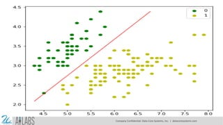
![Next, we can evaluate the model and plot it as follows:
model = LogisticRegression(lr=0.1, num_iter=300000)
preds = model.predict(X) # how well our predictions work
(preds == y).mean()
plt.figure(figsize=(10, 6))
plt.scatter(X[y == 0][:, 0], X[y == 0][:, 1], color='g', label='0')
plt.scatter(X[y == 1][:, 0], X[y == 1][:, 1], color='y', label='1') plt.legend()
x1_min, x1_max = X[:,0].min(), X[:,0].max(),
x2_min, x2_max = X[:,1].min(), X[:,1].max(),
xx1, xx2 = np.meshgrid(np.linspace(x1_min, x1_max), np.linspace(x2_min, x2_max))
grid = np.c_[xx1.ravel(), xx2.ravel()]
probs = model.predict_prob(grid).reshape(xx1.shape) plt.contour(xx1, xx2, probs, [0.5],
linewidths=1, colors='red');
Company Confidential: Data-Core Systems, Inc. | datacoresystems.com](https://image.slidesharecdn.com/machinelearningwithpython-machinelearningalgorithms-logisticregression-250217162710-8d34f275/85/Machine-Learning-with-Python-Machine-Learning-Algorithms-Logistic-Regression-pdf-14-320.jpg)
![cm = confusion_matrix(y, model.predict(X))
fig, ax = plt.subplots(figsize=(8, 8))
ax.imshow(cm)
ax.grid(False)
ax.xaxis.set(ticks=(0, 1), ticklabels=('Predicted 0s', 'Predicted 1s'))
ax.yaxis.set(ticks=(0, 1), ticklabels=('Actual 0s', 'Actual 1s'))
ax.set_ylim(1.5, -0.5)
for i in range(2):
for j in range(2):
ax.text(j, i, cm[i, j], ha='center', va='center', color='white')
plt.show()
Company Confidential: Data-Core Systems, Inc. | datacoresystems.com](https://image.slidesharecdn.com/machinelearningwithpython-machinelearningalgorithms-logisticregression-250217162710-8d34f275/85/Machine-Learning-with-Python-Machine-Learning-Algorithms-Logistic-Regression-pdf-17-320.jpg)


Machine Learning with Python- Machine Learning Algorithms- Logistic Regression.pdf
- 1. Machine Learning with Python Machine Learning Algorithms - Logistic Regression Prof.ShibdasDutta, Associate Professor, DCGDATACORESYSTEMSINDIAPVTLTD Kolkata Company Confidential: Data-Core Systems, Inc. | datacoresystems.com
- 2. Machine Learning Algorithms – Classification Algo- Logistic Regression Logistic Regression - Introduction Logistic regression is a supervised learning classification algorithm used to predict the probability of a target variable. The nature of target or dependent variable is dichotomous, which means there would be only two possible classes. In simple words, the dependent variable is binary in nature having data coded as either 1 (stands for success/yes) or 0 (stands for failure/no). Mathematically, a logistic regression model predicts P(Y=1) as a function of X. It is one of the simplest ML algorithms that can be used for various classification problems such as spam detection, Diabetes prediction, cancer detection etc. Company Confidential: Data-Core Systems, Inc. | datacoresystems.com
- 3. Types of Logistic Regression Generally, logistic regression means binary logistic regression having binary target variables, but there can be two more categories of target variables that can be predicted by it. Based on those number of categories, Logistic regression can be divided into following types: Binary or Binomial In such a kind of classification, a dependent variable will have only two possible types either 1 and 0. For example, these variables may represent success or failure, yes or no, win or loss etc. Multinomial In such a kind of classification, dependent variable can have 3 or more possible unordered types or the types having no quantitative significance. For example, these variables may represent “Type A” or “Type B” or “Type C”. Ordinal In such a kind of classification, dependent variable can have 3 or more possible ordered types or the types having a quantitative significance. For example, these variables may represent “poor” or “good”, “very good”, “Excellent” and each category can have the scores like 0,1,2,3.
- 4. Logistic Regression Assumptions Before diving into the implementation of logistic regression, we must be aware of the following assumptions about the same: • In case of binary logistic regression, the target variables must be binary always and the desired outcome is represented by the factor level 1. • There should not be any multi-collinearity in the model, which means the independent variables must be independent of each other. • We must include meaningful variables in our model. • We should choose a large sample size for logistic regression. Company Confidential: Data-Core Systems, Inc. | datacoresystems.com
- 5. Binary Logistic Regression model The simplest form of logistic regression is binary or binomial logistic regression in which the target or dependent variable can have only 2 possible types either 1 or 0. It allows us to model a relationship between multiple predictor variables and a binary/binomial target variable. In case of logistic regression, the linear function is basically used as an input to another function such as g in the following relation: Here, g is the logistic or sigmoid function. To sigmoid curve can be represented with the help of following graph. We can see the values of y-axis lie between 0 and 1 and crosses the axis at 0.5. Hypothesis , e is the natural log 2.718 The classes can be divided into positive or negative. The output comes under the probability of positive class if it lies between 0 and 1. For our implementation, we are interpreting the output of hypothesis function as positive if it is ≥ 0.5, otherwise negative.
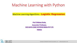
- 6. We also need to define a loss function to measure how well the algorithm performs using the weights on functions, represented by theta as follows: Loss function Functions have parameters/weights (represented by theta in our notation) and we want to find the best values for them. To start we pick random values and we need a way to measure how well the algorithm performs using those random weights. That measure is computed using the loss function, defined as: def loss(h, y): return (-y * np.log(h) - (1 - y) * np.log(1 - h)).mean() Company Confidential: Data-Core Systems, Inc. | datacoresystems.com
- 7. Now, after defining the loss function our prime goal is to minimize the loss function. It can be done with the help of fitting the weights which means by increasing or decreasing the weights. With the help of derivatives of the loss function w.r.t each weight, we would be able to know what parameters should have high weight and what should have smaller weight. Gradient descent The following gradient descent equation tells us how loss would change if we modified the parameters: Partial derivative gradient = np.dot(X.T, (h - y)) / y.shape[0] Then we update the weights by substracting to them the derivative times the learning rate. lr = 0.01 theta -= lr * gradient We should repeat this steps several times until we reach the optimal solution. Company Confidential: Data-Core Systems, Inc. | datacoresystems.com
- 8. Predictions By calling the sigmoid function we get the probability that some input x belongs to class 1. Let’s take all probabilities ≥ 0.5 = class 1 and all probabilities < 0 = class 0. This threshold should be defined depending on the business problem we were working. def predict_probs(X, theta): return sigmoid(np.dot(X, theta))def predict(X, theta, threshold=0.5): return predict_probs(X, theta) >= threshold Company Confidential: Data-Core Systems, Inc. | datacoresystems.com
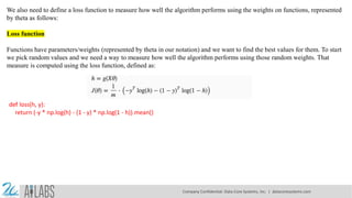
- 9. Implementation in Python Now we will implement the above concept of binomial logistic regression in Python. For this purpose, we are using a multivariate flower dataset named ‘iris’ which have 3 classes of 50 instances each, but we will be using the first two feature columns. Every class represents a type of iris flower. First, we need to import the necessary libraries as follows: import numpy as np import matplotlib.pyplot as plt import seaborn as sns from sklearn import datasets Next, load the iris dataset as follows: iris = datasets.load_iris() X = iris.data[:, :2] y = (iris.target != 0) * 1 We can plot our training data s follows: Weather it can be separated with decision boundary or not? plt.figure(figsize=(10, 6)) plt.scatter(X[y == 0][:, 0], X[y == 0][:, 1], color='g', label='0') plt.scatter(X[y == 1][:, 0], X[y == 1][:, 1], color='y', label='1') plt.legend();
- 10. It seems that it can be differentiated using a Decision Boundary, now lets define our class. Next, we will define sigmoid function, loss function and gradient descend as follows: Company Confidential: Data-Core Systems, Inc. | datacoresystems.com
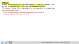
- 11. class LogisticRegression: #defining parameters such as learning rate, number ot iterations, whether to include intercept, # and verbose which says whether to print anything or not like, loss etc. def init (self, lr=0.01, num_iter=100000, fit_intercept=True, verbose=False): self.lr = lr self.num_iter = num_iter self.fit_intercept = fit_intercept self.verbose = verbose def add_intercept(self, X): # function to define the Incercept value. intercept = np.ones((X.shape[0], 1)) # initially we set it as all 1's # then we concatinate them to the value of X, we don't add we just append them at the end. return np.concatenate((intercept, X), axis=1) def sigmoid(self, z): # this is our actual sigmoid function which predicts our yp return 1 / (1 + np.exp(-z)) def loss(self, h, y): # this is the loss function which we use to minimize the error of our model return (-y * np.log(h) - (1 - y) * np.log(1 - h)).mean() def fit(self, X, y): # this is the function which trains our model. if self.fit_intercept: X = self. add_intercept(X) # as said if we want our intercept term to be added we use fit_intercept=True
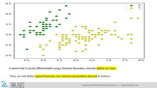
- 12. Now, initialize the weights as follows: self.theta = np.zeros(X.shape[1]) # weights initialization of our Normal Vector, initially we set it to 0, then we learn it eventually for i in range(self.num_iter): # this for loop runs for the number of iterations provided z = np.dot(X, self.theta) # this is our theta * Xi h = self. sigmoid(z) # this is where we predict the values of Y based on theta and Xi gradient = np.dot(X.T, (h - y)) / y.size # this is where the gradient is calculated form the error generated by our model self.theta -= self.lr * gradient # this is where we update our values of theta, so that we can use the new values for the next iteration z = np.dot(X, self.theta) # this is our new theta * Xi h = self. sigmoid(z) loss = self. loss(h, y) # this is where the loss is calculated if(self.verbose ==True and i % 10000 == 0): # as mentioned above if we want to print somehting we use verbose, so if verbose=True then our loss get printed print(f'loss: {loss} t') Company Confidential: Data-Core Systems, Inc. | datacoresystems.com
- 13. With the help of the following script, we can predict the output probabilities: # this is where we predict the probability values based on out generated W values out of all those iterations. def predict_prob(self, X): # as said if we want our intercept term to be added we use fit_intercept=True if self.fit_intercept: X = self. add_intercept(X) # this is the final prediction that is generated based on the values learned. return self. sigmoid(np.dot(X, self.theta)) # this is where we predict the actual values 0 or 1 using round. anything less than 0.5 = 0 or more than 0.5 is 1 def predict(self, X): return self.predict_prob(X).round() Company Confidential: Data-Core Systems, Inc. | datacoresystems.com
- 14. Next, we can evaluate the model and plot it as follows: model = LogisticRegression(lr=0.1, num_iter=300000) preds = model.predict(X) # how well our predictions work (preds == y).mean() plt.figure(figsize=(10, 6)) plt.scatter(X[y == 0][:, 0], X[y == 0][:, 1], color='g', label='0') plt.scatter(X[y == 1][:, 0], X[y == 1][:, 1], color='y', label='1') plt.legend() x1_min, x1_max = X[:,0].min(), X[:,0].max(), x2_min, x2_max = X[:,1].min(), X[:,1].max(), xx1, xx2 = np.meshgrid(np.linspace(x1_min, x1_max), np.linspace(x2_min, x2_max)) grid = np.c_[xx1.ravel(), xx2.ravel()] probs = model.predict_prob(grid).reshape(xx1.shape) plt.contour(xx1, xx2, probs, [0.5], linewidths=1, colors='red'); Company Confidential: Data-Core Systems, Inc. | datacoresystems.com
- 15. Company Confidential: Data-Core Systems, Inc. | datacoresystems.com
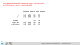
- 16. from sklearn.metrics import classification_report, confusion_matrix print(classification_report(y, model.predict(X))) precision recall f1-score support 0 1.00 1.00 1.00 50 1 1.00 1.00 1.00 100 accuracy 1.00 150 macro avg 1.00 1.00 1.00 150 weighted avg 1.00 1.00 1.00 150 Company Confidential: Data-Core Systems, Inc. | datacoresystems.com
- 17. cm = confusion_matrix(y, model.predict(X)) fig, ax = plt.subplots(figsize=(8, 8)) ax.imshow(cm) ax.grid(False) ax.xaxis.set(ticks=(0, 1), ticklabels=('Predicted 0s', 'Predicted 1s')) ax.yaxis.set(ticks=(0, 1), ticklabels=('Actual 0s', 'Actual 1s')) ax.set_ylim(1.5, -0.5) for i in range(2): for j in range(2): ax.text(j, i, cm[i, j], ha='center', va='center', color='white') plt.show() Company Confidential: Data-Core Systems, Inc. | datacoresystems.com
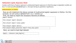
- 18. Multinomial Logistic Regression Model Another useful form of logistic regression is multinomial logistic regression in which the target or dependent variable can have 3 or more possible unordered types i.e. the types having no quantitative significance. Implementation in Python Now we will implement the above concept of multinomial logistic regression in Python. For this purpose, we are using a dataset from sklearn named digit. First, we need to import the necessary libraries as follows: Import sklearn from sklearn import datasets from sklearn import linear_model from sklearn import metrics from sklearn.model_selection import train_test_split Next, we need to load digit dataset: digits = datasets.load_digits() Company Confidential: Data-Core Systems, Inc. | datacoresystems.com
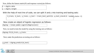
- 19. Now, define the feature matrix(X) and response vector(y)as follows: X = digits.data y = digits.target With the help of next line of code, we can split X and y into training and testing sets: X_train, X_test, y_train, y_test = train_test_split(X, y,test_size=0.4, random_state= 1) Now create an object of logistic regression as follows: digreg = linear_model.LogisticRegression() Now, we need to train the model by using the training sets as follows: digreg.fit(X_train, y_train) Next, make the predictions on testing set as follows: y_pred = digreg.predict(X_test) Company Confidential: Data-Core Systems, Inc. | datacoresystems.com
- 20. Next print the accuracy of the model as follows: print("Accuracy of Logistic Regression model is:", metrics.accuracy_score(y_test, y_pred)*100) Output Accuracy of Logistic Regression model is: 95.6884561891516 From the above output we can see the accuracy of our model is around 96 percent. Company Confidential: Data-Core Systems, Inc. | datacoresystems.com
- 21. Thank You Company Confidential: Data-Core Systems, Inc. | datacoresystems.com