
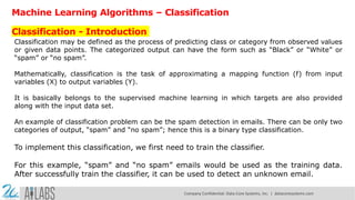
![We also need to organize the data and it can be done with the help of following scripts:
label_names = data['target_names']
labels = data['target']
feature_names = data['feature_names']
features = data['data']
The following command will print the name of the labels, ‘malignant’ and ‘benign’ in case of our database.
print(label_names)
The output of the above command is the names of the labels:
['malignant' 'benign']
These labels are mapped to binary values 0 and 1. Malignant cancer is represented by 0
and Benign cancer is represented by 1.
The feature names and feature values of these labels can be seen with the help
of following commands:
Company Confidential: Data-Core Systems, Inc. | datacoresystems.com](https://image.slidesharecdn.com/machinelearningwithpython-machinelearningalgorithms-250217162712-4ef490a9/85/Machine-Learning-with-Python-Machine-Learning-Algorithms-pdf-5-320.jpg)
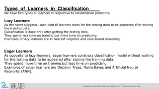
![print(feature_names[0])
The output of the above command is the names of the features for label 0 i.e. Malignant
cancer:
mean radius
Similarly, names of the features for label can be produced as follows:
print(feature_names[1])
The output of the above command is the names of the features for label 1 i.e. Benign
cancer:
mean texture
We can print the features values for these labels with the help of following command:
print(features[0])
Company Confidential: Data-Core Systems, Inc. | datacoresystems.com](https://image.slidesharecdn.com/machinelearningwithpython-machinelearningalgorithms-250217162712-4ef490a9/85/Machine-Learning-with-Python-Machine-Learning-Algorithms-pdf-6-320.jpg)
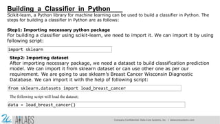
![This will give the following output:
[1.799e+01 1.038e+01 1.228e+02 1.001e+03 1.184e-01 2.776e-01 3.001e-01 1.471e-01
2.419e-01 7.871e-02 1.095e+00 9.053e-01 8.589e+00 1.534e+02
6.399e-03 4.904e-02 5.373e-02 1.587e-02 3.003e-02 6.193e-03 2.538e+01
1.733e+01 1.846e+02 2.019e+03 1.622e-01 6.656e-01 7.119e-01 2.654e-01
4.601e-01 1.189e-01]
We can print the features values for these labels with the help of following command:
print(features[1])
This will give the following output:
[2.057e+01 1.777e+01 1.329e+02 1.326e+03 8.474e-02 7.864e-02 8.690e-02 7.017e-02
1.812e-01 5.667e-02 5.435e-01 7.339e-01 3.398e+00 7.408e+01
5.225e-03 1.308e-02 1.860e-02 1.340e-02 1.389e-02 3.532e-03 2.499e+01
2.341e+01 1.588e+02 1.956e+03 1.238e-01 1.866e-01 2.416e-01 1.860e-01
2.750e-01 8.902e-02]
Company Confidential: Data-Core Systems, Inc. | datacoresystems.com](https://image.slidesharecdn.com/machinelearningwithpython-machinelearningalgorithms-250217162712-4ef490a9/85/Machine-Learning-with-Python-Machine-Learning-Algorithms-pdf-7-320.jpg)
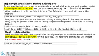
![Now, initialize the model as follows:
gnb = GaussianNB()
Next, with the help of following command we can train the model:
model = gnb.fit(train, train_labels)
Now, for evaluation purpose we need to make predictions. It can be done by using
predict() function as follows:
preds = gnb.predict(test)
print(preds)
This will give the following output: [1 0 0 1 1 0 0 0 1 1 1 0 1 0 1 0 1 1 1 0 1 10 1 1 11 11 0 11 111 10
1 0 1 1 0 1 1 1 1 1 1 1 1 0 0 1 1 1 1 1 0 0 1 1 0 0 1 1 1 0 0 1 1 0 0 1 0
1 1 1 1 1 1 0 1 1 0 0 0 0 0 1 1 1 1 1 1 1 1 0 0 1 0 0 1 0 0 1 1 1 0 1 1 0
1 1 0 0 0 1 1 1 0 0 1 1 0 1 0 0 1 1 0 0 0 1 1 1 0 1 1 0 0 1 0 1 1 0 1 0 0
1 1 1 1 1 1 1 0 0 1 1 1 1 1 1 1 1 1 1 1 1 0 1 1 1 0 1 1 0 1 1 1 1 1 1 0 0
0 1 1 0 1 0 1 1 1 1 0 1 1 0 1 1 1 0 1 0 0 1 1 1 1 1 1 1 1 0 1 1 1 1 1 0 1
0 0 1 1 0 1]
The above series of 0s and 1s in output are the predicted values for the Malignant and
Benign tumor classes
Company Confidential: Data-Core Systems, Inc. | datacoresystems.com](https://image.slidesharecdn.com/machinelearningwithpython-machinelearningalgorithms-250217162712-4ef490a9/85/Machine-Learning-with-Python-Machine-Learning-Algorithms-pdf-9-320.jpg)

![We can find the confusion matrix with the help of confusion_matrix() function of sklearn. With the help of the
following script, we can find the confusion matrix of above built binary classifier:
from sklearn.metrics import confusion_matrix
Output
[[ 73 7]
[ 4 144]]
Accuracy
It may be defined as the number of correct predictions made by our ML model. We can easily
calculate it by confusion matrix with the help of following formula:
Accuracy = (TP+TN) / (TP+FP+FN+TN)
For above built binary classifier, TP + TN = 73+144 = 217 and TP+FP+FN+TN =
73+7+4+144=228.
Hence, Accuracy = 217/228 = 0.951754385965 which is same as we have
calculated after creating our binary classifier.
Company Confidential: Data-Core Systems, Inc. | datacoresystems.com](https://image.slidesharecdn.com/machinelearningwithpython-machinelearningalgorithms-250217162712-4ef490a9/85/Machine-Learning-with-Python-Machine-Learning-Algorithms-pdf-13-320.jpg)


Machine Learning with Python- Machine Learning Algorithms.pdf
- 1. Machine Learning with Python Machine Learning Algorithms Prof.ShibdasDutta, Associate Professor, DCGDATACORESYSTEMSINDIAPVTLTD Kolkata Company Confidential: Data-Core Systems, Inc. | datacoresystems.com
- 2. Machine Learning Algorithms – Classification Classification - Introduction Classification may be defined as the process of predicting class or category from observed values or given data points. The categorized output can have the form such as “Black” or “White” or “spam” or “no spam”. Mathematically, classification is the task of approximating a mapping function (f) from input variables (X) to output variables (Y). It is basically belongs to the supervised machine learning in which targets are also provided along with the input data set. An example of classification problem can be the spam detection in emails. There can be only two categories of output, “spam” and “no spam”; hence this is a binary type classification. To implement this classification, we first need to train the classifier. For this example, “spam” and “no spam” emails would be used as the training data. After successfully train the classifier, it can be used to detect an unknown email. Company Confidential: Data-Core Systems, Inc. | datacoresystems.com
- 3. Types of Learners in Classification We have two types of learners in respective to classification problems: Lazy Learners As the name suggests, such kind of learners waits for the testing data to be appeared after storing the training data. Classification is done only after getting the testing data. They spend less time on training but more time on predicting. Examples of lazy learners are K- nearest neighbor and case-based reasoning. Eager Learners As opposite to lazy learners, eager learners construct classification model without waiting for the testing data to be appeared after storing the training data. They spend more time on training but less time on predicting. Examples of eager learners are Decision Trees, Naïve Bayes and Artificial Neural Networks (ANN). Company Confidential: Data-Core Systems, Inc. | datacoresystems.com
- 4. Building a Classifier in Python Scikit-learn, a Python library for machine learning can be used to build a classifier in Python. The steps for building a classifier in Python are as follows: Step1: Importing necessary python package For building a classifier using scikit-learn, we need to import it. We can import it by using following script: import sklearn Step2: Importing dataset After importing necessary package, we need a dataset to build classification prediction model. We can import it from sklearn dataset or can use other one as per our requirement. We are going to use sklearn’s Breast Cancer Wisconsin Diagnostic Database. We can import it with the help of following script: from sklearn.datasets import load_breast_cancer The following script will load the dataset; data = load_breast_cancer() Company Confidential: Data-Core Systems, Inc. | datacoresystems.com
- 5. We also need to organize the data and it can be done with the help of following scripts: label_names = data['target_names'] labels = data['target'] feature_names = data['feature_names'] features = data['data'] The following command will print the name of the labels, ‘malignant’ and ‘benign’ in case of our database. print(label_names) The output of the above command is the names of the labels: ['malignant' 'benign'] These labels are mapped to binary values 0 and 1. Malignant cancer is represented by 0 and Benign cancer is represented by 1. The feature names and feature values of these labels can be seen with the help of following commands: Company Confidential: Data-Core Systems, Inc. | datacoresystems.com
- 6. print(feature_names[0]) The output of the above command is the names of the features for label 0 i.e. Malignant cancer: mean radius Similarly, names of the features for label can be produced as follows: print(feature_names[1]) The output of the above command is the names of the features for label 1 i.e. Benign cancer: mean texture We can print the features values for these labels with the help of following command: print(features[0]) Company Confidential: Data-Core Systems, Inc. | datacoresystems.com
- 7. This will give the following output: [1.799e+01 1.038e+01 1.228e+02 1.001e+03 1.184e-01 2.776e-01 3.001e-01 1.471e-01 2.419e-01 7.871e-02 1.095e+00 9.053e-01 8.589e+00 1.534e+02 6.399e-03 4.904e-02 5.373e-02 1.587e-02 3.003e-02 6.193e-03 2.538e+01 1.733e+01 1.846e+02 2.019e+03 1.622e-01 6.656e-01 7.119e-01 2.654e-01 4.601e-01 1.189e-01] We can print the features values for these labels with the help of following command: print(features[1]) This will give the following output: [2.057e+01 1.777e+01 1.329e+02 1.326e+03 8.474e-02 7.864e-02 8.690e-02 7.017e-02 1.812e-01 5.667e-02 5.435e-01 7.339e-01 3.398e+00 7.408e+01 5.225e-03 1.308e-02 1.860e-02 1.340e-02 1.389e-02 3.532e-03 2.499e+01 2.341e+01 1.588e+02 1.956e+03 1.238e-01 1.866e-01 2.416e-01 1.860e-01 2.750e-01 8.902e-02] Company Confidential: Data-Core Systems, Inc. | datacoresystems.com
- 8. Step3: Organizing data into training & testing sets As we need to test our model on unseen data, we will divide our dataset into two parts: a training set and a test set. We can use train_test_split() function of sklearn python package to split the data into sets. The following command will import the function: from sklearn.model_selection import train_test_split Now, next command will split the data into training & testing data. In this example, we are using taking 40 percent of the data for testing purpose and 60 percent of the data for training purpose: train, test, train_labels, test_labels = train_test_split(features,labels,test_size = 0.40, random_state = 42) Step4- Model evaluation After dividing the data into training and testing we need to build the model. We will be using Naïve Bayes algorithm for this purpose. The following commands will import the GaussianNB module: from sklearn.naive_bayes import GaussianNB Company Confidential: Data-Core Systems, Inc. | datacoresystems.com
- 9. Now, initialize the model as follows: gnb = GaussianNB() Next, with the help of following command we can train the model: model = gnb.fit(train, train_labels) Now, for evaluation purpose we need to make predictions. It can be done by using predict() function as follows: preds = gnb.predict(test) print(preds) This will give the following output: [1 0 0 1 1 0 0 0 1 1 1 0 1 0 1 0 1 1 1 0 1 10 1 1 11 11 0 11 111 10 1 0 1 1 0 1 1 1 1 1 1 1 1 0 0 1 1 1 1 1 0 0 1 1 0 0 1 1 1 0 0 1 1 0 0 1 0 1 1 1 1 1 1 0 1 1 0 0 0 0 0 1 1 1 1 1 1 1 1 0 0 1 0 0 1 0 0 1 1 1 0 1 1 0 1 1 0 0 0 1 1 1 0 0 1 1 0 1 0 0 1 1 0 0 0 1 1 1 0 1 1 0 0 1 0 1 1 0 1 0 0 1 1 1 1 1 1 1 0 0 1 1 1 1 1 1 1 1 1 1 1 1 0 1 1 1 0 1 1 0 1 1 1 1 1 1 0 0 0 1 1 0 1 0 1 1 1 1 0 1 1 0 1 1 1 0 1 0 0 1 1 1 1 1 1 1 1 0 1 1 1 1 1 0 1 0 0 1 1 0 1] The above series of 0s and 1s in output are the predicted values for the Malignant and Benign tumor classes Company Confidential: Data-Core Systems, Inc. | datacoresystems.com
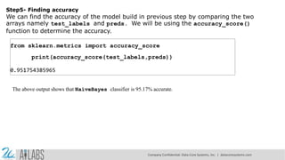
- 10. Step5- Finding accuracy We can find the accuracy of the model build in previous step by comparing the two arrays namely test_labels and preds. We will be using the accuracy_score() function to determine the accuracy. from sklearn.metrics import accuracy_score print(accuracy_score(test_labels,preds)) 0.951754385965 The above output shows that NaïveBayes classifier is 95.17% accurate. Company Confidential: Data-Core Systems, Inc. | datacoresystems.com
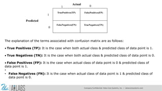
- 11. Classification Evaluation Metrics The job is not done even if you have finished implementation of your Machine Learning application or model. We must have to find out how effective our model is? There can be different evaluation metrics, but we must choose it carefully because the choice of metrics influences how the performance of a machine learning algorithm is measured and compared. The following are some of the important classification evaluation metrics among which you can choose based upon your dataset and kind of problem: Confusion Matrix It is the easiest way to measure the performance of a classification problem where the output can be of two or more type of classes. A confusion matrix is nothing but a table with two dimensions viz. “Actual” and “Predicted” and furthermore, both the dimensions have “True Positives (TP)”, “True Negatives (TN)”, “False Positives (FP)”, “False Negatives (FN)” as shown below: Company Confidential: Data-Core Systems, Inc. | datacoresystems.com
- 12. The explanation of the terms associated with confusion matrix are as follows: True Positives (TP): It is the case when both actual class & predicted class of data point is 1. True Negatives (TN): It is the case when both actual class & predicted class of data point is 0. False Positives (FP): It is the case when actual class of data point is 0 & predicted class of data point is 1. • • False Negatives (FN): It is the case when actual class of data point is 1 & predicted class of data point is 0. TruePositives(TP) FalsePositives(FP) FalseNegatives(FN) TrueNegatives(TN) Actual 1 0 1 0 Predicted Company Confidential: Data-Core Systems, Inc. | datacoresystems.com
- 13. We can find the confusion matrix with the help of confusion_matrix() function of sklearn. With the help of the following script, we can find the confusion matrix of above built binary classifier: from sklearn.metrics import confusion_matrix Output [[ 73 7] [ 4 144]] Accuracy It may be defined as the number of correct predictions made by our ML model. We can easily calculate it by confusion matrix with the help of following formula: Accuracy = (TP+TN) / (TP+FP+FN+TN) For above built binary classifier, TP + TN = 73+144 = 217 and TP+FP+FN+TN = 73+7+4+144=228. Hence, Accuracy = 217/228 = 0.951754385965 which is same as we have calculated after creating our binary classifier. Company Confidential: Data-Core Systems, Inc. | datacoresystems.com
- 14. Precision Precision, used in document retrievals, may be defined as the number of correct documents returned by our ML model. We can easily calculate it by confusion matrix with the help of following formula: Precision = TP / (TP+FP) For the above built binary classifier, TP = 73 and TP+FP = 73+7 = 80. Hence, Precision = 73/80 = 0.915 Recall or Sensitivity Recall may be defined as the number of positives returned by our ML model. We can easily calculate it by confusion matrix with the help of following formula: Recall = TP / (TP + FN) For above built binary classifier, TP = 73 and TP+FN = 73+4 = 77. Hence, Precision = 73/77 = 0.94805 Specificity Specificity, in contrast to recall, may be defined as the number of negatives returned by our ML model. We can easily calculate it by confusion matrix with the help of following formula: Specificity = TN / (TN+FP) For the above built binary classifier, TN = 144 and TN+FP = 144+7 = 151. Hence, Precision = 144/151 = 0.95364 Company Confidential: Data-Core Systems, Inc. | datacoresystems.com
- 15. Applications Some of the most important applications of classification algorithms are as follows: Speech Recognition Handwriting Recognition Biometric Identification • Document Classification Company Confidential: Data-Core Systems, Inc. | datacoresystems.com
- 16. Thank You Company Confidential: Data-Core Systems, Inc. | datacoresystems.com