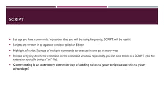
SlideShare a Scribd company logo
MATLAB :TUTORIAL 1 (INTRO)
GETTINGYOURSELVES FAMILIAR
WORRY NOT, IT IS NOT AS HARD ASYOU THINK
DOWNLOAD
MATLAB
1. Click and submit Uni name and your
university email
https://www.mathworks.com/prod
ucts/get-
matlab.html?s_tid=gn_getml
2. Click to download
MATLAB
ENVIRONMENT
 Command Window
 Workspace
 Current Folder
 Command History
 Click “Layout” if you do not
have them
CURRENT FOLDER
 Shows the current folder you are in / where your files will be saved,
display all files in the current folder
 GOOD HABIT: Keep a pendrive around, and store the directory you
made specifically for this class in there
 Proper naming scheme of your files is important
 e.g. tutorial_1_intro_week4.m
 Only those in bold can be read by MATLAB
COMMAND WINDOW
 Type all your command/lines of the programming
 The results/variables typed in command window will be saved in WORKSPACE
WORKSPACE
 Store all your variables from your command window or the script.
 You may choose to save the variables by
- right-clicking theWorkspace >> save – To save ALLVariables
- choose variables >> right-click >> save as –To save SelectedVariables
 ‘clear all’ will clear all the unsaved variables in Workspace (or select all variable, and delete)
 IMPORTANT: Create your own personal directory (folder) where you will store all your contents
 The SavedWorkspace variables will be visible in current folder (in a .mat file)
 When saving matlab files, the name CANNOT contain space. (use underscore instead)
COMMAND HISTORY
 Store the commands you typed in command window
 You may directly copy the command and turn them into Script / Live Script
 Live Script : interactive documents that combine MATLAB code with formatted text, equations, and images in a
single environment called the Live Editor. In addition, live scripts store and display output alongside the code
that creates it.
 Highlight of command history: For keeping track of previous commands, and restoration in case of accidental
deletion
NOTE: If command history box is not visible,
HOME >> Environment >>Layout >> Command History >> Select ‘Docked’
SCRIPT
 Let say you have commands / equations that you will be using frequently, SCRIPT will be useful.
 Scripts are written in a separate window called an Editor
 Highlight of script: Storage of multiple commands to execute in one go, in many ways
 Instead of typing down the command in the command window repeatedly, you can save them in a SCRIPT (the file
extension typically being a “.m” file).
 Commenting is an extremely common way of adding notes to your script; abuse this to your
advantage!
RECAP
 Command Window
 Workspace
 Current Folder
 Command History
 MATLAB Intro (ALL)
 Script
FURTHER REFERENCES
 MATLAB Onramp, a tutorial service for getting used to the basic features in MATLAB
(requires signup of email)
MATLAB :TUTORIAL
(SIMULINK)
WHAT IS SIMULINK?
 A graphical programming environment that utilizes
blocks.
 Used for simulations, development, and analysis in an
intuitive flowchart-like manner.
 Typically requires a lot of memory allocation, which
means you need to wait some time for it to become
fast and responsive (or just use SSD).
LAUNCH SIMULINK
1st way : Click this icon,
then select ‘Blank Model’
2nd way :
i. type slLibraryBrowser
ii. Click this →
SIMULINK INTERFACE
Open new
blank Simulink
Simulation time
Block library Run
simulation
BASIC PURPOSES OF SIMULINK BLOCKS
 INPUT
 The starting point of your simulations, located in “Sources” within the Simulink Library. Can be considered an “activator” to any
process or function.
 Examples: Constant value, step (single magnitude) input, ramp (steady) input, sinusoidal signal input, repeated sequence,
imported data from spreadsheet, etc.
 PROCESS
 Has a slot for input and output, modifies the input into a specific output value.Also has auxiliary uses.
 Examples:Transfer function, equation, controller, simple math operation, etc.
 OUTPUT
 What comes out of a process. Depending on the type of process, it can be in many forms.
 A value, a graph, another process (equation), a variable to export into workspace, etc.
 Related to this lesson however, the output blocks located in “Sinks” within the library are used.
TASK 1 : LET’S TRY
Let’s simulate two simple math problems:
And show the answer in a “Display” block.
1. Load the inputs.The two inputs used are simple constant values, within “Sources”.
- Drag and drop the block from the library, and place into an open Simulink environment.
- Access the block’s properties (double click), and change it to what we need.
2. Load the process to use our two inputs.As it is a simple addition, what we want can be found under “Math
Operations”.
3. Connect the two inputs to the process that we want to run them through.
4. Select the “Display” block within “Sinks” and connect the output of the operation to it.
5. Repeat steps for second math problem.
i. 𝟏 + 𝟐
ii. 20 - 12
PROTIPS
 Size not to your liking?You can increase/decrease the environment size with mousewheel drag
up/down. For a MUCH MORE pleasant navigational and working experience, use the middle
mousewheel click + drag to pan across the space.
 The interface is flexible.You can copy, cut and paste, comment out any unneeded blocks.
 Typical keyboard shortcuts also applies (for copying, pasting, etc).
 You can rename the blocks by clicking on it, and then clicking the name space below it.
 The blocks themselves are flexible in application. For example;
- The “Add” block is not just for additions.You can alter the properties within, to change into
another operational block (without having to open another one in the library), and even include
more options.
- Can change the addition to subtraction, multiplication to divison, etc., and even add in more input
slots!
- It is possible to connect 1 variable for multiple blocks/operations (treat it as if it’s a single variable).
With the right mouse click, this can be done much easier.
i. 𝟏 + 𝟐
ii. 20 - 12
TRICYCLE RUN (TUTORIAL TASK 1)
THIS ISYOUR REPLACEMENTTASK 1 FORTHETUTORIAL
Save everything from previous slides, and create a new Simulink file.
Let’s simulate 4 simple math operations within a fresh new Simulink file,
and show the answer in multiple “Display” blocks:
1. 15 + 2 + 4 = 21
2. 46/2 = 23
3. 15*4 = 60
4. 15*2+46 =76
REALIZING THE TRANSFER FUNCTION COMPONENTS
Remember the definitions to each term?
K = gain of process (proportional value that shows the relationship between the magnitude of the input to the
magnitude of the output signal at steady state)
𝜏 = process time constant (time takes for process to reach 63.2% of its total change)
𝜃 = process time delay
We will now see how it is tangible in describing transfer function behaviour!
𝐺(𝑠) =
𝐾
𝜏𝑠 + 1
𝑒−𝜃𝑠 𝐺(𝑠) =
2
10𝑠 + 1
𝑒−5𝑠
TRANSFER FUNCTIONS IN SIMULINK
𝐺(𝑠) =
2
10𝑠 + 1
𝑒−5𝑠
Let’s create TF in Simulink, and observe
its response to a step input at t = 5, with magnitude of 2.
Open up a new Simulink file.
1. Within “Continuous” section in Library, select “Transfer Fcn”. Drop it into your blank
Simulink file.
2. Edit the properties of the numerator
and denominator to match what we want
above
(double click/open and change the
properties).
MATLAB simulink open loop dynamics system
TRANSFER FUNCTIONS IN SIMULINK
To observe the step response… we need a step input, and export the visual as a graph.
4. Under “Sources”, select “Step” block. Add in Simulink, and change the initial and final values to generate a
magnitude of 2. NOTE: You don’t change the “step time” option to get a magnitude change.
TRANSFER FUNCTIONS IN SIMULINK
5. Under “Sinks”, select “Scope” block. Add in Simulink, link everything together, and run.
6. Double-click the Scope to see the graph. Did it display everything you expected it to show?
TRANSFER FUNCTIONS IN SIMULINK
7. As a general rule of thumb, set the simulation time to be higher than 9x the process time constant. For this
example, just set it as 100.
TRANSFER FUNCTIONS IN SIMULINK
LET’S PRACTICE :
1. Try ramp input and observe response 2. Try sine wave input and observe response
2ND ORDERTRANSFER FUNCTION
𝐺(𝑠) =
2
𝑠2 + 10𝑠 + 1
𝑒−5𝑠
Let’s create 2nd order TF in Simulink, and observe
its response to a step input at t = 5, with magnitude of 2.
1. Within “Continuous” section in Library, select “Transfer Fcn”. Drop it into your blank
Simulink file.
2. Edit the properties of the numerator
and denominator to match what we want
above
(double click/open and change the
properties).
𝐺(𝑠) =
2
𝑠2 + 10𝑠 + 1
𝑒−5𝑠
2ND ORDERTRANSFER FUNCTION
𝐺(𝑠) =
2
𝑠2 + 10𝑠 + 1
𝑒−5𝑠
4. Under “Sources”, select “Step” block. Add in Simulink, and change the initial and final values to generate a
magnitude of 2.
2ND ORDERTRANSFER FUNCTION
5. Under “Sinks”, select “Scope” block. Add in Simulink, link everything together, and run.
6. Double-click the Scope to see the graph. Discuss your observations.
2ND ORDERTRANSFER FUNCTION
LET’S PRACTICE FOR 2ND ORDER TF :
1. Try ramp input and observe response 2. Try sine wave input and observe response
CONCLUSION
CONCLUSION
CONCLUSION
MATLAB :TUTORIAL 2
(TRANSFER FUNCTIONS)
BASIC COMPONENTS OF A 1ST ORDERTRANSFER FUNCTION
In the standard form, these are what each terms stand for:
K = gain of process
𝜏 = process time constant (time takes for process to reach 63.2% of its total change)
𝜃 = process time delay
𝐺(𝑠) =
𝐾
𝜏𝑠 + 1
𝑒−𝜃𝑠
TRANSFER FUNCTION CREATION
How to create transfer function?
Let’s create:
1. Define numerator, e.g.
>> num = [10]
2. Define denominator, e.g.
>> den = [7 1]
3. Use “tf” command, with the following function,
>> G = tf(num,den)
4. Observe the step response with,
>> step(G)
𝐺(𝑠) =
10
7𝑠 + 1
TRANSFER FUNCTION DELAY ADDITION
How to add a delay to the transfer function?
Let’s make it as such:
1. Duplicate the transfer function to be created,
>> Gd = G
2. Observe all the editable variables with,
>> get(Gd)
3. Change the specific variable to the value we want.
In this case, it’s the OutputDelay,and we change it with,
>> set(Gd,‘OutputDelay’, 8)
4. Observe the newly delayed step response with,
>> step(Gd)
𝐺𝑑(𝑠) =
10
7𝑠 + 1
𝑒−8𝑠
ADDITIONAL MATLAB COMMANDS
How to create a simple graph?
 Use “plot” command
 A simple demo, enter the following in your MATLAB command window:
>> a = [1:1:100];
>> plot(a);
ADDITIONAL MATLAB COMMANDS
How to create multiple graphs?
 Command “figure” is used to pre-generate a “canvas”
 Enter the following in your MATLAB command window:
>> a = [1:1:100];
>> b = [3:3:300];
>> figure;
>> plot(a);
>> figure;
>> plot(b);
ADDITIONAL MATLAB COMMANDS
How to overlay multiple plots in one figure?
 For quick application, use “hold” command
 “hold on” to enable overlaying of future plots into a single figure,“hold off” to continue making plots in additional figures
 Using the same variables as before as an example:
>> a = [1:1:100];
>> b = [3:3:300];
>> figure;
>> plot(a);
>> hold on
>> plot(b,”x”);
>> hold off
LET’S GO TOTHE TUTORIALS
 Final result that I want from the developed script:
- Creates all the required variables in the workspace.
- Automatically generates 6 separate plots.
- DOES NOT touch any ofTasks 1.d, 1.e, 2.c, 2d.
Ad

Recommended

Mit6 094 iap10_lec05
Tribhuwan Pant
 
Simulink
Simulink
jackabraham
 
Simulink Presentation.ppt
hodeeeeee1
 
ADVANCED WORKSHOP IN MATLAB
Saeed J. Almalowi,PhD
 
learn matlab for ease Lec5
Amba Research
 
Simulink4 beginners
Simulink4 beginners
sandeep2506
 
Simulink 1.pdf
Simulink 1.pdf
ssuser1dfd371
 
1.1Introduction to matlab.pptx
BeheraA
 
Summer training matlab
Arshit Rai
 
EE6711 Power System Simulation Lab manual
Velalar College of Engineering and Technology
 
Introduction to matlab
VidhyaSenthil
 
M3M_250327ggggt_224420_250411_183353.pdf
HebaEng
 
Summer training matlab
Arshit Rai
 
Simulink
Simulink
Kelin Jose
 
Control system Lab record
Yuvraj Singh
 
Control chap9
Control chap9
Mohd Ashraf Shabarshah
 
MATLAB/SIMULINK for Engineering Applications day 2:Introduction to simulink
reddyprasad reddyvari
 
Forelasning4
Forelasning4
Memo Love
 
Mmc manual
Mmc manual
Urvi Surat
 
Malab tutorial
Malab tutorial
sisira senarathna
 
Matlab 1 level_1
Matlab 1 level_1
Ahmed Farouk
 
10_Matlab Simulink for Electrical Engineering.pptx
RomanusPeterLyanda
 
Introduction to MATLAB 7 - WIlliam PALM III.ppt
HassenMOuakkad
 
Matlab workshop
Matlab workshop
محمدعبد الحى
 
++Matlab 14 sesiones
Rosemberth Rodriguez
 
simulink
simulink
Aditi Tiwari
 
The speed of the motor has been varied successfully in a
MuhZakaria1
 
Simulation lab
Simulation lab
Ezhilarasi Nagarajan
 
Research Proposal Writing and thesispptx
sirisha n
 
Cover page analysis for optimum conditions
sirisha n
 

More Related Content

Similar to MATLAB simulink open loop dynamics system (20)

Summer training matlab
Arshit Rai
 
EE6711 Power System Simulation Lab manual
Velalar College of Engineering and Technology
 
Introduction to matlab
VidhyaSenthil
 
M3M_250327ggggt_224420_250411_183353.pdf
HebaEng
 
Summer training matlab
Arshit Rai
 
Simulink
Simulink
Kelin Jose
 
Control system Lab record
Yuvraj Singh
 
Control chap9
Control chap9
Mohd Ashraf Shabarshah
 
MATLAB/SIMULINK for Engineering Applications day 2:Introduction to simulink
reddyprasad reddyvari
 
Forelasning4
Forelasning4
Memo Love
 
Mmc manual
Mmc manual
Urvi Surat
 
Malab tutorial
Malab tutorial
sisira senarathna
 
Matlab 1 level_1
Matlab 1 level_1
Ahmed Farouk
 
10_Matlab Simulink for Electrical Engineering.pptx
RomanusPeterLyanda
 
Introduction to MATLAB 7 - WIlliam PALM III.ppt
HassenMOuakkad
 
Matlab workshop
Matlab workshop
محمدعبد الحى
 
++Matlab 14 sesiones
Rosemberth Rodriguez
 
simulink
simulink
Aditi Tiwari
 
The speed of the motor has been varied successfully in a
MuhZakaria1
 
Simulation lab
Simulation lab
Ezhilarasi Nagarajan
 
Summer training matlab
Arshit Rai
 
Introduction to matlab
VidhyaSenthil
 
M3M_250327ggggt_224420_250411_183353.pdf
HebaEng
 
Summer training matlab
Arshit Rai
 
Control system Lab record
Yuvraj Singh
 
MATLAB/SIMULINK for Engineering Applications day 2:Introduction to simulink
reddyprasad reddyvari
 
Forelasning4
Forelasning4
Memo Love
 
10_Matlab Simulink for Electrical Engineering.pptx
RomanusPeterLyanda
 
Introduction to MATLAB 7 - WIlliam PALM III.ppt
HassenMOuakkad
 
The speed of the motor has been varied successfully in a
MuhZakaria1
 

More from sirisha n (7)

Research Proposal Writing and thesispptx
sirisha n
 
Cover page analysis for optimum conditions
sirisha n
 
new developments in intelleuctual proeprty
sirisha n
 
industrial effluent andwaste water residues
sirisha n
 
ICARE technology and innovation in teaching
sirisha n
 
Technical writing in research methodology
sirisha n
 
technical Writing for research methodology
sirisha n
 
Ad

Recently uploaded (20)

Rapid Prototyping for XR: Lecture 1 Introduction to Prototyping
Mark Billinghurst
 
System design handwritten notes guidance
Shabista Imam
 
تقرير عن التحليل الديناميكي لتدفق الهواء حول جناح.pdf
محمد قصص فتوتة
 
Introduction to Python Programming Language
merlinjohnsy
 
International Journal of Advanced Information Technology (IJAIT)
ijait
 
May 2025: Top 10 Read Articles in Data Mining & Knowledge Management Process
IJDKP
 
AI_Presentation (1). Artificial intelligence
RoselynKaur8thD34
 
Bitumen Emulsion by Dr Sangita Ex CRRI Delhi
grilcodes
 
FSE-Journal-First-Automated code editing with search-generate-modify.pdf
cl144
 
20CE404-Soil Mechanics - Slide Share PPT
saravananr808639
 
Proposal for folders structure division in projects.pdf
Mohamed Ahmed
 
Deep Learning for Image Processing on 16 June 2025 MITS.pptx
resming1
 
Complete guidance book of Asp.Net Web API
Shabista Imam
 
NEW Strengthened Senior High School Gen Math.pptx
DaryllWhere
 
Call For Papers - 17th International Conference on Wireless & Mobile Networks...
hosseinihamid192023
 
Industrial internet of things IOT Week-3.pptx
KNaveenKumarECE
 
Rapid Prototyping for XR: Lecture 2 - Low Fidelity Prototyping.
Mark Billinghurst
 
Industry 4.o the fourth revolutionWeek-2.pptx
KNaveenKumarECE
 
Generative AI & Scientific Research : Catalyst for Innovation, Ethics & Impact
AlqualsaDIResearchGr
 
دراسة حاله لقرية تقع في جنوب غرب السودان
محمد قصص فتوتة
 
Ad

MATLAB simulink open loop dynamics system

  • 1. MATLAB :TUTORIAL 1 (INTRO) GETTINGYOURSELVES FAMILIAR GETTINGYOURSELVES FAMILIAR WORRY NOT, IT IS NOT AS HARD ASYOU THINK
  • 2. DOWNLOAD MATLAB 1. Click and submit Uni name and your university email https://www.mathworks.com/prod ucts/get- matlab.html?s_tid=gn_getml 2. Click to download
  • 3. MATLAB ENVIRONMENT  Command Window  Workspace  Current Folder  Command History  Click “Layout” if you do not have them
  • 4. CURRENT FOLDER  Shows the current folder you are in / where your files will be saved, display all files in the current folder  GOOD HABIT: Keep a pendrive around, and store the directory you made specifically for this class in there  Proper naming scheme of your files is important  e.g. tutorial_1_intro_week4.m  Only those in bold can be read by MATLAB
  • 5. COMMAND WINDOW  Type all your command/lines of the programming  The results/variables typed in command window will be saved in WORKSPACE
  • 6. WORKSPACE  Store all your variables from your command window or the script.  You may choose to save the variables by - right-clicking theWorkspace >> save – To save ALLVariables - choose variables >> right-click >> save as –To save SelectedVariables  ‘clear all’ will clear all the unsaved variables in Workspace (or select all variable, and delete)  IMPORTANT: Create your own personal directory (folder) where you will store all your contents  The SavedWorkspace variables will be visible in current folder (in a .mat file)  When saving matlab files, the name CANNOT contain space. (use underscore instead)
  • 7. COMMAND HISTORY  Store the commands you typed in command window  You may directly copy the command and turn them into Script / Live Script  Live Script : interactive documents that combine MATLAB code with formatted text, equations, and images in a single environment called the Live Editor. In addition, live scripts store and display output alongside the code that creates it.  Highlight of command history: For keeping track of previous commands, and restoration in case of accidental deletion NOTE: If command history box is not visible, HOME >> Environment >>Layout >> Command History >> Select ‘Docked’
  • 8. SCRIPT  Let say you have commands / equations that you will be using frequently, SCRIPT will be useful.  Scripts are written in a separate window called an Editor  Highlight of script: Storage of multiple commands to execute in one go, in many ways  Instead of typing down the command in the command window repeatedly, you can save them in a SCRIPT (the file extension typically being a “.m” file).  Commenting is an extremely common way of adding notes to your script; abuse this to your advantage!
  • 9. RECAP  Command Window  Workspace  Current Folder  Command History  MATLAB Intro (ALL)  Script
  • 10. FURTHER REFERENCES  MATLAB Onramp, a tutorial service for getting used to the basic features in MATLAB (requires signup of email)
  • 12. WHAT IS SIMULINK?  A graphical programming environment that utilizes blocks.  Used for simulations, development, and analysis in an intuitive flowchart-like manner.  Typically requires a lot of memory allocation, which means you need to wait some time for it to become fast and responsive (or just use SSD).
  • 13. LAUNCH SIMULINK 1st way : Click this icon, then select ‘Blank Model’ 2nd way : i. type slLibraryBrowser ii. Click this →
  • 14. SIMULINK INTERFACE Open new blank Simulink Simulation time Block library Run simulation
  • 15. BASIC PURPOSES OF SIMULINK BLOCKS  INPUT  The starting point of your simulations, located in “Sources” within the Simulink Library. Can be considered an “activator” to any process or function.  Examples: Constant value, step (single magnitude) input, ramp (steady) input, sinusoidal signal input, repeated sequence, imported data from spreadsheet, etc.  PROCESS  Has a slot for input and output, modifies the input into a specific output value.Also has auxiliary uses.  Examples:Transfer function, equation, controller, simple math operation, etc.  OUTPUT  What comes out of a process. Depending on the type of process, it can be in many forms.  A value, a graph, another process (equation), a variable to export into workspace, etc.  Related to this lesson however, the output blocks located in “Sinks” within the library are used.
  • 16. TASK 1 : LET’S TRY Let’s simulate two simple math problems: And show the answer in a “Display” block. 1. Load the inputs.The two inputs used are simple constant values, within “Sources”. - Drag and drop the block from the library, and place into an open Simulink environment. - Access the block’s properties (double click), and change it to what we need. 2. Load the process to use our two inputs.As it is a simple addition, what we want can be found under “Math Operations”. 3. Connect the two inputs to the process that we want to run them through. 4. Select the “Display” block within “Sinks” and connect the output of the operation to it. 5. Repeat steps for second math problem. i. 𝟏 + 𝟐 ii. 20 - 12
  • 17. PROTIPS  Size not to your liking?You can increase/decrease the environment size with mousewheel drag up/down. For a MUCH MORE pleasant navigational and working experience, use the middle mousewheel click + drag to pan across the space.  The interface is flexible.You can copy, cut and paste, comment out any unneeded blocks.  Typical keyboard shortcuts also applies (for copying, pasting, etc).  You can rename the blocks by clicking on it, and then clicking the name space below it.  The blocks themselves are flexible in application. For example; - The “Add” block is not just for additions.You can alter the properties within, to change into another operational block (without having to open another one in the library), and even include more options. - Can change the addition to subtraction, multiplication to divison, etc., and even add in more input slots! - It is possible to connect 1 variable for multiple blocks/operations (treat it as if it’s a single variable). With the right mouse click, this can be done much easier. i. 𝟏 + 𝟐 ii. 20 - 12
  • 18. TRICYCLE RUN (TUTORIAL TASK 1) THIS ISYOUR REPLACEMENTTASK 1 FORTHETUTORIAL Save everything from previous slides, and create a new Simulink file. Let’s simulate 4 simple math operations within a fresh new Simulink file, and show the answer in multiple “Display” blocks: 1. 15 + 2 + 4 = 21 2. 46/2 = 23 3. 15*4 = 60 4. 15*2+46 =76
  • 19. REALIZING THE TRANSFER FUNCTION COMPONENTS Remember the definitions to each term? K = gain of process (proportional value that shows the relationship between the magnitude of the input to the magnitude of the output signal at steady state) 𝜏 = process time constant (time takes for process to reach 63.2% of its total change) 𝜃 = process time delay We will now see how it is tangible in describing transfer function behaviour! 𝐺(𝑠) = 𝐾 𝜏𝑠 + 1 𝑒−𝜃𝑠 𝐺(𝑠) = 2 10𝑠 + 1 𝑒−5𝑠
  • 20. TRANSFER FUNCTIONS IN SIMULINK 𝐺(𝑠) = 2 10𝑠 + 1 𝑒−5𝑠 Let’s create TF in Simulink, and observe its response to a step input at t = 5, with magnitude of 2. Open up a new Simulink file. 1. Within “Continuous” section in Library, select “Transfer Fcn”. Drop it into your blank Simulink file.
  • 21. 2. Edit the properties of the numerator and denominator to match what we want above (double click/open and change the properties).
  • 23. TRANSFER FUNCTIONS IN SIMULINK To observe the step response… we need a step input, and export the visual as a graph. 4. Under “Sources”, select “Step” block. Add in Simulink, and change the initial and final values to generate a magnitude of 2. NOTE: You don’t change the “step time” option to get a magnitude change.
  • 24. TRANSFER FUNCTIONS IN SIMULINK 5. Under “Sinks”, select “Scope” block. Add in Simulink, link everything together, and run. 6. Double-click the Scope to see the graph. Did it display everything you expected it to show?
  • 25. TRANSFER FUNCTIONS IN SIMULINK 7. As a general rule of thumb, set the simulation time to be higher than 9x the process time constant. For this example, just set it as 100.
  • 26. TRANSFER FUNCTIONS IN SIMULINK LET’S PRACTICE : 1. Try ramp input and observe response 2. Try sine wave input and observe response
  • 27. 2ND ORDERTRANSFER FUNCTION 𝐺(𝑠) = 2 𝑠2 + 10𝑠 + 1 𝑒−5𝑠 Let’s create 2nd order TF in Simulink, and observe its response to a step input at t = 5, with magnitude of 2. 1. Within “Continuous” section in Library, select “Transfer Fcn”. Drop it into your blank Simulink file.
  • 28. 2. Edit the properties of the numerator and denominator to match what we want above (double click/open and change the properties). 𝐺(𝑠) = 2 𝑠2 + 10𝑠 + 1 𝑒−5𝑠 2ND ORDERTRANSFER FUNCTION
  • 29. 𝐺(𝑠) = 2 𝑠2 + 10𝑠 + 1 𝑒−5𝑠
  • 30. 4. Under “Sources”, select “Step” block. Add in Simulink, and change the initial and final values to generate a magnitude of 2. 2ND ORDERTRANSFER FUNCTION
  • 31. 5. Under “Sinks”, select “Scope” block. Add in Simulink, link everything together, and run. 6. Double-click the Scope to see the graph. Discuss your observations. 2ND ORDERTRANSFER FUNCTION
  • 32. 2ND ORDERTRANSFER FUNCTION LET’S PRACTICE FOR 2ND ORDER TF : 1. Try ramp input and observe response 2. Try sine wave input and observe response
  • 37. BASIC COMPONENTS OF A 1ST ORDERTRANSFER FUNCTION In the standard form, these are what each terms stand for: K = gain of process 𝜏 = process time constant (time takes for process to reach 63.2% of its total change) 𝜃 = process time delay 𝐺(𝑠) = 𝐾 𝜏𝑠 + 1 𝑒−𝜃𝑠
  • 38. TRANSFER FUNCTION CREATION How to create transfer function? Let’s create: 1. Define numerator, e.g. >> num = [10] 2. Define denominator, e.g. >> den = [7 1] 3. Use “tf” command, with the following function, >> G = tf(num,den) 4. Observe the step response with, >> step(G) 𝐺(𝑠) = 10 7𝑠 + 1
  • 39. TRANSFER FUNCTION DELAY ADDITION How to add a delay to the transfer function? Let’s make it as such: 1. Duplicate the transfer function to be created, >> Gd = G 2. Observe all the editable variables with, >> get(Gd) 3. Change the specific variable to the value we want. In this case, it’s the OutputDelay,and we change it with, >> set(Gd,‘OutputDelay’, 8) 4. Observe the newly delayed step response with, >> step(Gd) 𝐺𝑑(𝑠) = 10 7𝑠 + 1 𝑒−8𝑠
  • 40. ADDITIONAL MATLAB COMMANDS How to create a simple graph?  Use “plot” command  A simple demo, enter the following in your MATLAB command window: >> a = [1:1:100]; >> plot(a);
  • 41. ADDITIONAL MATLAB COMMANDS How to create multiple graphs?  Command “figure” is used to pre-generate a “canvas”  Enter the following in your MATLAB command window: >> a = [1:1:100]; >> b = [3:3:300]; >> figure; >> plot(a); >> figure; >> plot(b);
  • 42. ADDITIONAL MATLAB COMMANDS How to overlay multiple plots in one figure?  For quick application, use “hold” command  “hold on” to enable overlaying of future plots into a single figure,“hold off” to continue making plots in additional figures  Using the same variables as before as an example: >> a = [1:1:100]; >> b = [3:3:300]; >> figure; >> plot(a); >> hold on >> plot(b,”x”); >> hold off
  • 43. LET’S GO TOTHE TUTORIALS  Final result that I want from the developed script: - Creates all the required variables in the workspace. - Automatically generates 6 separate plots. - DOES NOT touch any ofTasks 1.d, 1.e, 2.c, 2d.