


![4
Introduction and
Acknowledgment
This text is about recursive algorithms. Therefore we must define what such
an algorithm is. An algorithm is called recursive, if it contains at least one
function which calls itself. A well-known and simple example is the compu-
tation of factorials. n! stands for the product of the integer numbers from 1
to n. But usually factorials are defined recursively, and 0! = 1 is also defined.
n! =
(
n · (n − 1)! if n > 0
1 if n = 0
.
This definition can easily be converted into a Python function:
def fakrek(n):
if n == 0: return 1
else: return n*fakrek(n-1)
However, it is not necessary to write your own function. Predefined functions
for factorials are available in modules math and scipy.
Some basic knowledge of Python is provided in this text. If you are an
absolute beginner you should study a tutorial on Python first. There you
will learn how to code loops with for or while and how to deal with func-
tions. It is not necessary to study the programming of classes; they will not
occur in this text because the codes are as simple as possible.
There are some examples in the following text which use turtlegraphics. Orig-
inally this kind of graphics was developed for the programming language Logo
[2]. The turtle was a small robot that could be directed to move around by
typing commands on the keyboard. But soon it appeared on the screen.
Turtlegraphics is also available in Python’s module turtle [3]. This kind of
graphics allows numerous nice examples which use recursions, and you can
watch how the graphics develops on the screen.](https://image.slidesharecdn.com/recursivealgorithmsr-250126092011-2b54067b/85/Recursive-Algorithms-coded-in-Python-pdf-5-320.jpg)
![Introduction 5
Whenever a drawing with turtlegraphics is finished the program should re-
turn to the editor. But to achieve this may not be quite simple. We used
the version for PyCharm [4] in the programs treated below. For closing the
frame for turtlegraphics using Sypder [5] see appendix ”how to terminate
turtlegraphics under Spyder”. Nevertheless sometimes the simple version for
PyCharm also works with Spyder.
Chapter 1 starts with some examples of simple recursive algorithms. In
chapter 2 a couple of mathematical applications of recursions are described.
Chapter 3 is about recursive algorithms with more than one call. In that
chapter we shall see that recursive algorithms are not always advantageous,
and it may be better to use iterative algorithms instead. Finally, in chapter
4 some algorithms with indirect recursive calls are discussed.
There are some general programming concepts which are related with recur-
sive algorithms. ’Divide and Conquer’ divides the input into smaller and
smaller sub-problems until a trivial solution can be found for each. Then the
partial solutions are put together to yield a complete solution of the origi-
nal problem. Well-known examples are binary search, see Section 1.1.4, and
merge sort, see Section 3.4. Another concept is ’Branch and Bound’. There
the aim is to minimize the set of possible solutions. This is done by branch-
ing the set of feasible solutions into subsets and installing suitable bounds.
A typical example is solving integer linear problems, see Section 3.7. ’Back-
tracking’ is a concept which is especially useful for constraint satisfaction
problems e.g, for the knapsack problem, see Section 3.6.
The programs discussed are coded in a rather simple manner. Certainly
experts would code some of them shorter and in a more elegant way. But
in this text comprehensibility was emphasized most. Modules for diverse
purposes have been created for Python during last years. So many of the
problems discussed in this text can easily be solved applying one of these
modules. But here only such modules are used that are included in the
Python package except turtle and scipy for ILP (Section 3.7).
The codes were written in Python 3.9.13 [1] and tested with 3.11.5 and 3.13.
Meanwhile there will be more recent versions, and it is possible that some
parts of the codes will not work any more. But in most cases it will not be
difficult to update the codes.
The program scripts and the solutions of the exercises can be found in [82].
Many thanks to Horst Oehr for reading the text and testing the codes.](https://image.slidesharecdn.com/recursivealgorithmsr-250126092011-2b54067b/85/Recursive-Algorithms-coded-in-Python-pdf-6-320.jpg)
![6
Chapter 1
Simple Recursions
1.1 Some Examples for Beginners
1.1.1 Harmonic Series
The harmonic series is defined by
1 +
1
2
+
1
3
+
1
4
+ ... =
∞
X
n=1
1
n
Every added fraction is smaller than the preceding one. But the value of
partial sums
HN =
N
X
n=1
1
n
(1.1)
grows slowly with increasing N. In the 14th century the french philosopher
Nicole Oresme showed that the partial sums diverge [6]. That means they
grow infinitely with increasing N. But actually N must be large to surpass
even a relatively small number such as 8. We develop a short program which
computes partial sums (Eq. (1.1)) of the harmonic series to explore the min-
imal N such that
PN
n=1
1
n
yields more than 8.
A suitable recursive function is very simple:
def harmrek(n):
if n == 1: return 1
else: return harmrek(n-1) + 1/n
The computation of the partial sum with upper bound n is reduced to com-
puting it with the upper bound n-1 and adding 1
n
. If n = 1, 1 is returned.](https://image.slidesharecdn.com/recursivealgorithmsr-250126092011-2b54067b/85/Recursive-Algorithms-coded-in-Python-pdf-7-320.jpg)
![1.1. SOME EXAMPLES FOR BEGINNERS 7
The main program essentially consists of just two lines:
n = int(input(’n = ’))
print(’H(’,n,’) = ’,harmrek(n))
The function input interprets any input as a string. We have to convert it
into an integer number. That is why we must surround the call of input by
int(...). The second line shows the upper limit n and the resulting partial
sum.
The harmonic partial sums can be approximated by ln n + γ, where γ is
the Euler-Mascheroni constant which has the value γ ≈ 0.5772 [7]. In order
to compare our results with the approximation we must import the module
math at the beginning. The constant γ must be defined, and one more line
is added to the main program:
print(’approximated by’,math.log(n)+ gamma)
The function log of the module math computes the natural logarithm of the
argument.
The approximation is the better the greater n is. Here are two examples:
H( 10 ) = 2.9289682539682538, approximated by 2.879800757896
H( 1000 ) = 7.485470860550343, approximated by 7.48497094388367
Applying the approximation yields that to surpass the partial sum 8 you
must set n ≈ 1673. Using this program you can easily find the exact solu-
tion. Do not try much larger numbers. Otherwise the program will not work
and you’ll get the error message: RecursionError: maximum recursion
depth exceeded in comparison. There are some internet sites on the limit
of recursions in Python. Most of them state that it is 1000. You can find
out what the maximum recursion depth on your system really is. Just type
this small program and run it:
import sys
print(sys.getrecursionlimit())
It is even possible to change the limit of recursions on your system. However,
according to experts this is not recommended.
1.1.2 Hexagons
This is a little program showing some features of turtlegraphics. An overview
with all possibilities of turtlegraphics in Python can be found here [3]. We
should like to plot some regular hexagons which all have the same center.
The edges of each succeeding hexagon shall be shorter than the edges of the](https://image.slidesharecdn.com/recursivealgorithmsr-250126092011-2b54067b/85/Recursive-Algorithms-coded-in-Python-pdf-8-320.jpg)


![1.1. SOME EXAMPLES FOR BEGINNERS 10
tu.setpos(-0.5*a,-0.866*a)
tu.down()
for i in range(6):
tu.forward(a); tu.left(60)
tu.up(); tu.setpos(0,0)
if a > 25: hexagon(a*0.8, red, blue)
Now let us take a glance at the main program. The colors have to be ini-
tialized: red = 1; blue = 0.2, and the width of the pen is fixed such that
is not too small: tu.pensize(width = 3). Then the essential function is
called: hexagon(200,red,blue). At last there are some lines to announce to
the user that the drawing is finished. Finally we have to care that the panel
of turtlegraphics can be closed properly. Here the version for PyCharm [4]
is presented; for Spyder [5] see terminate turtlegraphics with Spyder. Here
is the complete main program:
red = 1; blue = 0.2
tu.pensize(width = 3)
hexagon(200,red, blue)
tu.up(); tu.hideturtle()
tu.setpos(-300,-250); tu.pencolor((0,0,0))
tu.write(’finished!’,font = ("Arial",12,"normal"))
tu.exitonclick() # für PyCharm
try:tu.bye()
except tu.Terminator: pass
The following figure 1.3 shows the first three steps of the concentric hexagons
described above.
Figure 1.3: First three hexagons, colors intensified](https://image.slidesharecdn.com/recursivealgorithmsr-250126092011-2b54067b/85/Recursive-Algorithms-coded-in-Python-pdf-11-320.jpg)
![1.1. SOME EXAMPLES FOR BEGINNERS 11
1.1.3 Palindromes
If a word is equal to its reverse it is called a palindrome, for example ”level”.
A palindrome can also be a number, such as 43134 or a short phrase like ”no
melon no lemon”. In this case spaces between the words are ignored. We
intend to develop a small program to check whether or not a given string is
a palindrome.
For that it is useful to define ”palindrome” in a different way [8]:
A string P is called palindrome,
ˆ if it contains at most one character
ˆ or if the string P’ is a palindrome where P’ is obtained from P by
cancelling the first and the last character.
This characterization permits to develop a recursive function isPalindrome
which does the above checking. In the code of this function p assigns the
result, i.e. True or False. The value of p is returned to the function by
which isPalindrome is called. The if-branch is very simple. len(st) is the
length of string st. If it is at most 1, st is a palindrome.
The else-branch is not so simple. Assume our string is ’RADAR’. Python
allows access to each character, where the characters are numbered beginning
with 0. For example st[2] = ’D’, st[0] = st[4] = ’R’. It is also possible to copy
parts of a string. The first three characters of st are obtained by st[:3],
thus st[:3] = ’RAD’. Generally st[:n] consists of the first n characters
of st. If you put a number before the colon, say st[n:], the characters of
st beginning with number n are copied. Example: st[2:] = ’DAR’. Our
function has to use the string without the first character, that is st[1:].
But how can we tell the program to cancel the last character too if we do
not know the length of st? Fortunately python provides negative indices.
st[1:-1] is string st without the first and the last character. (If we wanted
to cancel the last two characters, we would write st[1:-2].)
We want a recursive call isPalindrome(st[1:-1]) only if the shortened
string could still be a palindrome. Thus before the call the first and last
character have to be checked. If they are different, st[0] != st[-1], p is
set False. Otherwise the recursive call is processed. Here is the listing:
def isPalindrome(st):
if len(st) <= 1: p = True
else:
if st[0] != st[-1]: p = False](https://image.slidesharecdn.com/recursivealgorithmsr-250126092011-2b54067b/85/Recursive-Algorithms-coded-in-Python-pdf-12-320.jpg)
![1.1. SOME EXAMPLES FOR BEGINNERS 12
else: p = isPalindrome(st[1:-1])
return p
There is one more function in our program: checkPalindrome(st). Its task
is to prepare the string, to call function isPalindrome and to display the
result. The line stu = st.upper() converts all characters to corresponding
capitals. For example st = ’Radar’ is converted to stu = ’RADAR’. The
following two lines remove spaces and commas by replacing them by ’’, the
empty string. (Similarly more special characters could be removed.) The
rest of the function is self-explanatory.
def checkPalindrome(st):
stu = st.upper()
stu = stu.replace(’ ’,’’)
print(st)
palin = isPalindrome(stu)
if palin == True:print(’is a palindrome.’)
else:print(’is not a palindrome.’)
print()
The main program is just one line, where checkPalindrom(st) is called.
But you can run this ”main program” several times with various strings, for
example
checkPalindrome(’noon’)
checkPalindrome(’rainbow’)
checkPalindrome(’Step on no pets’)
checkPalindrome(’borrow or rob’)
checkPalindrome(’12345321’)
Of course, two of these strings are no palindromes.
1.1.4 Binary Search
A frequent task in data processing is searching for certain data. The input
is a keyword or a number. The data processing program has to find the
corresponding data set or it has to tell the user that there is none. If the
keywords are not sorted the program must check every stored keyword. This
is very time-consuming. However, if the keywords are sorted much better
methods for searching are available. One of them is ”binary search” which
we demonstrate in this section.
Therefore a file with 1024 first names is loaded into the memory. We do not
discuss this part of the program because it has nothing to do with binary
search itself. The loaded names are stored in namesList.](https://image.slidesharecdn.com/recursivealgorithmsr-250126092011-2b54067b/85/Recursive-Algorithms-coded-in-Python-pdf-13-320.jpg)
![1.1. SOME EXAMPLES FOR BEGINNERS 13
The important function is search. It needs the two parameters l,r. These
are the left and right bound between which the search is performed. In
function search the variable found must be initialized. Then the mid-
dle m of l and r is determined: m = round((l+r)/2). The current name
namesList[m] is displayed so we can see what the function does. There are
three possibilities: (1) na == namesList[m] which means that name na was
found. In this case searching ends, and found = True and m are returned.
(2) The name na precedes namesList[m] in alphabetical order. In this case
also the condition l < m must be checked. If both conditions are fulfilled
searching continues in the interval [l,m-1]:
if (na < namesList[m]) & (l < m): found, m = search(l,m-1)
However, if the first condition is true but the second is not, the name na is
not in namesList. (3) The name na succeeds namesList[m] in alphabetical
order. This case is quite analogous to the second case. If m < r searching
continues in the right half of namesList, otherwise na cannot be found in
the list of names.
We must still explain why search has to return m and found. The reason
is that all variables in Python are local. Let us assume that na is found in
a certain recursive call of search. For example m = 47 and found = True.
These values are only ”known” to the current call of search. The copy
of search which called the version of search where na was found doesn’t
”know” anything about the successful search. That’s why we must return
parameters m and found to the calling copy of search. Here is the listing:
def search(l,r):
found = False
m = round((l+r)/2)
print(’ Name[’,m,’] = ’,namesList[m])
if na == namesList[m]: found = True
if (na < namesList[m]) & (l < m):found,m = search(l,m-1)
if (na > namesList[m]) & (m < r):found,m = search(m+1,r)
return found, m
Now, some words about the main program. Besides the header there is just
the input of the name na which is looked for. The call of function search
follows: found, m = search(0,n-1) The left and right limits are 0 and n-1,
these are the lowest and highest index of namesList. Finally the result is
displayed on the screen.
Why is ”binary search” advantageous? If a linear search in an unsorted
list of 1024 entries is carried out, the mean number of comparisons is 512.](https://image.slidesharecdn.com/recursivealgorithmsr-250126092011-2b54067b/85/Recursive-Algorithms-coded-in-Python-pdf-14-320.jpg)


![1.2. TOP-OF-STACK RECURSIONS 16
for i in range(n):
tu.forward(x); tu.right(angle)
x is the length of an edge. In the main program we set x = 360/n. count
denotes the number of calls needed to draw a complete rosette. After having
drawn a single polygon the turtle turns at a small angle: tu.right(7). The
last line is the recursive call: if count < 360/7:shape(count+1,x)
Figure 1.4: This rosette consists of pentagons.
That means that the length of an edge keeps its value, but variable count
is increased by one. So many polygons are drawn rotated by small angles,
and a rosette results. In total the code is very short and easy to understand.
Nevertheless it yields a result like figure 1.4.
1.2.3 Greatest Common Divisor
The greatest common divisor gcd of two (positive) numbers is the greatest
number by which both numbers can be divided without leaving a remainder.
Here we discuss a possibility to obtain the gcd of more than two numbers.
It applies the well-known Euclidean algorithm, see [9].
The main program is very short. The user is asked to enter at least two
numbers. The while-loops ensure that a or b cannot be 0. Then function](https://image.slidesharecdn.com/recursivealgorithmsr-250126092011-2b54067b/85/Recursive-Algorithms-coded-in-Python-pdf-17-320.jpg)
![1.3. EXERCISES 17
gcd is called, and that’s it. Here is the listing:
a, b = 0, 0
while a == 0:a = int(input(’first number: ’))
while b == 0:b = int(input(’second number: ’))
gcd(a,b)
In the function itself we take care that negative numbers can also be pro-
cessed. They are converted into positives if necessary.
if x < 0: x = -x; if y < 0: y = -y
Now four lines follow containing the Euclidean algorithm.
r = 1
while r > 0:
r = x % y; x = y; y = r
print(’The GCD is ’,x)
r denotes the remainder and is initially set to 1. The while-loop runs until r
is zero. The operation x % y computes the remainder obtained by dividing
x by y. x need not be greater than y. For example 5 % 7 = 5. Afterwards
the variables are shifted: x gets the value of y, and y is set to r. The proof
of correctness of the algorithm can be found in [9].
Next the user is asked to enter another number to continue the calculation
of the gcd.
z = int(input(’next number: ’))
if z != 0:gcd(x,z)
If 0 is entered the calculation is finished. Otherwise the gcd of the gcd ob-
tained so far and the new number is calculated. Here is an example. We want
to have the gcd of 525, 1365, 1015 and 749. Function gcd first returns 105 =
gcd(525,1365). Then 1015 is entered, and gcd(105,1015) = 35 is displayed.
After entering 749 the final result is gcd(35,749) = 7.
Since the recursive call is contained in the last line of the code of function
gcd it is a top-of-stack recursion.
1.3 Exercises
1. Alternating Harmonic Series
(i) Develop a program for computing partial sums of the alternating
harmonic series
1 −
1
2
+
1
3
−
1
4
+ −... =
∞
X
n=1
(−1)n+1 1
n](https://image.slidesharecdn.com/recursivealgorithmsr-250126092011-2b54067b/85/Recursive-Algorithms-coded-in-Python-pdf-18-320.jpg)
![1.3. EXERCISES 18
Your program should contain a recursive function. Additionally com-
pute the difference from ln 2 (that is np.log(2) in Python) which is
the limit of this series [10].
(ii) The alternating series
1 −
1
3
+
1
5
−
1
7
+ −... =
∞
X
n=0
(−1)n 1
2n + 1
has the limit π
4
[11]. Write a program that computes an approximation
for π using partial sums of the above series.
2. Snail-shell
Write a program which creates a drawing similar to figure 1.5. The
snail-shell consists of squares with decreasing edge lengths. There
are only two functions necessary to start and to stop filling a square:
tu.begin fill() and tu.end fill() before and after the code of the
drawing you want to fill. Hint: Red is coded by the triple (1,0,0), cyan
by (0,1,1).
Figure 1.5: Snail-shell with colors changing from red to cyan
3. Program X
Describe what functions work and work2 display on the screen and why
they do so. Which function is a top-of-stack recursion?](https://image.slidesharecdn.com/recursivealgorithmsr-250126092011-2b54067b/85/Recursive-Algorithms-coded-in-Python-pdf-19-320.jpg)
![1.3. EXERCISES 19
def work(k):
print(st[k],end = ’’)
if st[k] != ’ ’: work(k+1)
def work2(k):
if st[k] != ’ ’: work2(k+1)
print(st[k],end = ’’)
4. Snowflakes
A snowflake consists of a crystal containing several smaller sub-crystals
of the same shape as the first one. An elementary crystal is a star with
a certain number of rays. Create a program for drawing snowflakes
with at least 3 and at most 6 rays per star. Code a recursive function
applying turtlegraphics. The drawing may look like figure 1.6, see [12].
Figure 1.6: Snowflake - stars have five rays
Hints: The turtle moves forward from the center of the current star at
length x. Then function flake is called with parameter 0.4*x for five
or six rays, otherwise 0.5*x. When the function is finished the turtle
has to move back by x. To draw the next ray the turtle must turn at
angle 360°/n where n is the number of rays.](https://image.slidesharecdn.com/recursivealgorithmsr-250126092011-2b54067b/85/Recursive-Algorithms-coded-in-Python-pdf-20-320.jpg)

![21
Chapter 2
Some Recursive Algorithms in
Mathematics
There are a lot of recursive algorithms in mathematics. Only few of them
will be discussed here and coded in Python. An often represented example in
this context is the computation of Fibonacci numbers. But there are enough
of websites on this item [13]. More applications of recursions in mathematics
can be found in the next chapter because they are algorithms with more than
one recursive call.
2.1 Reducing Fractions
A fraction can be reduced by dividing the numerator and the denominator
by the greatest common divisor. However, normally reducing is not done
this way. Instead one tries to divide numerator and denominator by small
numbers as long as this is possible without leaving a remainder. Why not
try to code this method in Python?
We will not discuss the main program in detail. The numerator and the
denominator are entered, and they are expected to be positive. One more
variable is needed: prime = 2. And then the recursive call is done:
reduce(prime, num, den)
where num and den stand for numerator and denominator. prime denotes
a prime number. Initially prime is set to 2 which is the smallest prime. If
possible, num and den shall be divided by prime.
From function reduce first function search prime is called. It returns prime
and success. If the latter is True reducing of the fraction takes place: num
= num // prime and den = den // prime. The double slash stands for in-](https://image.slidesharecdn.com/recursivealgorithmsr-250126092011-2b54067b/85/Recursive-Algorithms-coded-in-Python-pdf-22-320.jpg)

![2.2. HERON’S METHOD 23
Now the program to reduce fractions in a special way is complete, and this
is an example for the output: 48/84 = 24/42 = 12/21 = 4/7.
2.2 Heron’s Method
Heron lived about 50 after Christ in Alexandria, Egypt [14]. He invented
a method for determining square roots approximately [15]. Let a be the
radicand. That is the number to determine the square root x of. Then
x =
√
a. x0 denotes the initial approximation, e.g. x0 = 1. Then we build
x1 =
1
2
· (x0 +
a
x0
)
Evidently, one of the numbers x0, a
x0
is greater and the other one is smaller
than
√
a. So x1 is a better approximation of
√
a than x0 because it is the
mean value of x0 and a
x0
. Again one of the numbers x1 and a
x1
is greater
than
√
a, and the other one is smaller. Thus we can continue and build
x2 = 1
2
· (x1 + a
x1
) and so on, in general
xi+1 =
1
2
· (xi +
a
xi
) (2.1)
But why do we know that the sequence < xi > really converges against
√
a?
It can easily be shown by solving a quadratic equation that for all natural
numbers i ∈ N:
xi >
√
a and
a
xi
<
√
a (2.2)
Since xi+1 < xi for all i the sequence < xi > is decreasing monotonously,
and the sequence < a
xi
> is increasing monotonously. Because of eq. (2.2)
the sequence of intervals [ a
xi
, xi] is an interval nesting and converges against
√
a. Now we are ready to implement Heron’s method. This is in fact not
very difficult. The main program is short and looks like this:
# main program
print("Computing Square Roots using Heron’s Method")
a = float(input(’radicant = ’))
d = int(input(’number of decimals: ’))
epsilon = 10**(-d)
Heron(1,0)](https://image.slidesharecdn.com/recursivealgorithmsr-250126092011-2b54067b/85/Recursive-Algorithms-coded-in-Python-pdf-24-320.jpg)
![2.3. CATALAN NUMBERS 24
Variable d denotes the accuracy of the desired approximation, and it is con-
verted to epsilon. At last function Heron is invoked with parameters 1 and
0. 1 is the zeroth approximation x0, and 0 the number of approximations.
Also function Heron looks very simple. First we increase i by one which
indicates the number of steps carried out. Then we apply eq. (2.2): x new =
0.5*(x + a/x) and the newly computed interval [ a
xi
, xi] is displayed. Finally
the recursive call has to be executed: if x new - a/x new > epsilon:
Heron(x new,i). That’s all. Here is the listing of the function:
def Heron(x,i):
i += 1
x new = 0.5*(x + a/x)
print(’step ’,i,’[’,a/x new,’,’,x new,’]’)
if x new - a/x new > epsilon:Heron(x new,i)
Heron’s method can easily be extended to an approximation of the kth root of
a given number. By applying the newton procedure for zeros on the function
f(x) = xk
− a it can be shown that eq. (2.2) has to be replaced by
xi+1 = (1 −
1
k
) · xi +
a
k · xk−1
i
(2.3)
The reader should implement a program using eq. (2.3) for approximating
kth roots. However, only approximations xi can be obtained, not intervals.
2.3 Catalan Numbers
Many a reader may not know what Catalan numbers are. Nevertheless they
play an important role in combinatorics. They are called after the Belgian
mathematician Eugène Catalan (1814-1894). There are two equivalent
definitions [16]:
Cn =
1
n + 1
·
2n
n
=
(2n)!
(n + 1)! · n!
(2.4)
But what are they good for? Here are some examples.
(1) Parentheses: A term like 18 − 9 − 4 − 1 makes no sense if there are no
parentheses set. There are some possibilities to set them. Here they are:
((18 − 9) − 4) − 1 = 4
(18 − (9 − 4)) − 1 = 12](https://image.slidesharecdn.com/recursivealgorithmsr-250126092011-2b54067b/85/Recursive-Algorithms-coded-in-Python-pdf-25-320.jpg)
![2.3. CATALAN NUMBERS 25
(18 − 9) − (4 − 1) = 6
18 − ((9 − 4) − 1) = 14
18 − (9 − (4 − 1)) = 12
Since there are three operations there are five possibilities to set parentheses,
and using eq. (2.4) it can easily be verified that C3 = 5. It can be shown
that the number of possible sets of parentheses in a term of n operations is
Cn, the Catalan number of n.
(2) The number of different binary trees with n nodes is Cn. Figure 2.1 shows
the non-isomorphic binary trees with three nodes. Notice that a branch or
leaf with a key smaller than the parent key is a ”left child”; if the key is
greater than the parent key it is a ”right child”. Therefore 1-2-3 and 3-2-1
are not isomorphic. The proof using eq. (2.5) is done in [17].
Figure 2.1: There are five non-isomorphic binary trees with three nodes.
(3) The number of non-crossing partitions of a set with n elements is Cn [18].
In Figure 2.2 C4 = 14 non-crossing partitions of the set consisting of four
elements is shown.
Indeed there are many more applications of Catalan numbers, but you can
see from the above examples how useful theses numbers are. But now we
will discuss three small programs for computing Catalan numbers in Python.
According to definition (2.4) we can implement a program which calls the
following recursive function for factorials three times:
def fakrek(n):
if n == 0:return 1
else:return n*fakrek(n-1)
The main program which computes Catalan numbers up to a limit n looks
like this:](https://image.slidesharecdn.com/recursivealgorithmsr-250126092011-2b54067b/85/Recursive-Algorithms-coded-in-Python-pdf-26-320.jpg)

![2.3. CATALAN NUMBERS 27
For tests you should enter small numbers such as 5 or 10. You will see
that the program works fine. You’ll see the Catalan numbers up to 5 or 10
on the screen, but if you enter somewhat larger numbers such as n = 18 you
will notice that the program gets slower and slower. The reason is that the
number of recursive calls increases exponentially. If you choose a still larger
n it may happen that the maximum depth for recursions does not suffice for
the required computation. The program is canceled and an error message is
displayed. That is not what we want.
How can we do better? We avoid the lots of recursive calls by introducing
a list, called CatList. The list must be initialized in the main program by
CatList = [ ]. The modified main program is not very complicated either.
We have just to append the current value of function Cat to our CatList.
Then the result can be displayed on the screen.
n = int(input(’limit = ’))
for i in range(n+1):
CatList.append(Cat(i,CatList))
print(’C(’,i,’) = ’,round(CatList[i]))
However, the function itself has to be modified. Instead of many recursive
calls the required Catalan numbers are obtained from CatList which is al-
ready filled as far as necessary. Thus the implementation of the function
looks like this:
def Cat(n,CatList):
if n == 0: return 1
else:
su = 0
for j in range(n):
su += CatList[j]*CatList[n-1-j]
return su
This program seems not to differ very much from the latter, but the most
important issue: There is no recursive call. Programs like these are called
iterative. The Catalan numbers obtained one after the other are stored in a
list or in an array. So they are available at once when needed.
Testing this iterative algorithm shows the enormous gain of speed. It costs
only a moment to get results like this C(40) = 2622127042276492108820. So
if you can convert a recursive algorithm into an iterative one the latter is
preferable. But this conversion is not always possible.](https://image.slidesharecdn.com/recursivealgorithmsr-250126092011-2b54067b/85/Recursive-Algorithms-coded-in-Python-pdf-28-320.jpg)
![2.4. BINOMIAL DISTRIBUTION 28
2.4 Binomial Distribution
Assume we have a box with w white and b black balls. A ball is randomly
drawn from the box n times, the color is checked, and then the ball is thrown
back into the box. We consider drawing of a white ball as ”success”. The
probability of success is p := w/(w + b). If a certain sequence of white and
black balls is fixed, the probability to draw k white balls is pk
· (1 − p)n−k
.
Let us consider an example with three white and five black balls. The prob-
ability to draw the sequence bbwbwwbb is (3
8
)3
· (5
8
)5
≈ 0.005. But if we
are not interested in the sequence of drawing white and black balls, and we
only consider the probability of obtaining k white balls, i.e. P(X = k),
we have to multiply the previous result with the number of possibilities to
choose k white balls of n. This number is the binomial coefficient n
k
[19].
So the number of successes is given by the so-called binomial distribution [20]:
p(X = k) =
n
k
· pk
· (1 − p)n−k
(2.6)
Let us look at the above example again. There are eight balls in a box, three
of them are white, and we draw eight times. The probability to draw three
white balls is according to eq. (2.6)
p(X = 3) =
8
3
· 0.3753
· 0.6255
≈ 0.2816
Eq. (2.6) can easily be implemented as a Python code because module scipy
provides a function which computes the binomial coefficients. The whole list-
ing is this:
import scipy.special as sp
headline and inputs
p = w/(w + b)
for k in range(n+1):
binom = sp.comb(n,k,exact = True)
binom = binom*(p**k)*((1-p)**(n-k))
print(’Probability for ’,k,’ white balls: ’,binom)
This is a short code which needs no recursion, but the predefined module
scipy instead. That is not really what we want. Instead we wish to create
a ”handmade” code with a recursive function. The for-loop of the main
program is shorter:](https://image.slidesharecdn.com/recursivealgorithmsr-250126092011-2b54067b/85/Recursive-Algorithms-coded-in-Python-pdf-29-320.jpg)
![2.4. BINOMIAL DISTRIBUTION 29
for k in range(n+1):
print(’Probability for ’,k,’ white balls: ’,prob(n,k))
Function prob has to be discussed. It starts with an if-clause: if (white
step) or (white 0):return 0. That is so because the number of white
balls cannot be greater than the number of draws and a negative number of
white balls doesn’t make sense. The first part of the else-branch contains
another if-clause: if step == 1:.... The if-branch consists of still one
more if-clause: if white == 1:return p, else:return 1-p. This case
covers the situation in which only one ball is drawn. The probability obtain-
ing a white ball is p, and the probability to draw a black ball is 1 − p. The
last else-branch is a bit complicated:
prob(1,0)*prob(step-1,white)+prob(1,1)*prob(step-1,white-1).
prob(1,0) can be replaced by 1-p, and prob(1,1) is the same as p. Ad-
ditionally there are two recursive function calls: prob(step-1,white) and
prob(step-1,white-1). To show the correctness we convert that line of the
Python code back into an algebraic formula.
P(X = k) =
n
k
· pk
(1 − p)n−k
=
(1 − p) ·
n − 1
k
· pk
(1 − p)n−1−k
+ p ·
n − 1
k − 1
· pk−1
(1 − p)n−k
We can rewrite this in the following way:
n
k
· pk
(1 − p)n−k
= pk
(1 − p)n−k
·
n − 1
k
+
n − 1
k − 1
This is equivalent to
n
k
= ·
n − 1
k
+
n − 1
k − 1
(2.7)
The proof of eq. (2.7) can be found in [21]. Thus we see that the last line of
function prob is indeed correct. So we show the whole listing.
def prob(step,white):
if (white step) or (white 0):return 0
else:
if step == 1:
if white == 1:return p
else:return 1 - p
else:](https://image.slidesharecdn.com/recursivealgorithmsr-250126092011-2b54067b/85/Recursive-Algorithms-coded-in-Python-pdf-30-320.jpg)


![2.5. DETERMINANTS 32
Here the parameters are are rank = 2, column = 2, ind = {2,3}. At this
step recursive calls end because a determinant with two rows can be com-
puted directly, see eq. 2.8. This is covered by the following part of det:
if rank == 2:
# find correct indices
k = list(ind)
if k[0] k[1]:x = k[0];k.pop(0);k.append(x)
res = A[k[0]][column]*A[k[1]][column+1]-
A[k[1]][column]*A[k[0]][column+1]
Finding the two correct indices looks a bit strange. Since we have to care
for the right order of the indices we need a list k with only two members. In
order to achieve that at first the set ind is converted to a list k. If the first
index is greater than the second, the first index is copied to x, then removed
from the list and x is appended at the end. Then the formula for two-rowed
determinants is applied.
The else-branch contains recursive calls. At first two local variables are
needed. res is reserved for the value of the current determinant. count
denotes a counter initialized with 0. It serves to ensure that the exponent in
eq. 2.10 is correct. Remember that the development of the determinant is
done by (current) column 0. So (-1)**count yields the correct sign. count
is not the same as i in the following for loop. Look at matrix 2.11 again. If
i = 1, subdeterminant
det
0 3 4
2 0 0
4 1 5
has to be computed. Therefore i obtains the values 0, 2, 3 one after the
other. But since count is local, it takes the values 0, 1 and 2.
The for-loop runs from 0 to n-1 and doesn’t care about the current rank. If
index i is in the current set ind of indices it must be removed from ind for
the following recursive call: ind=ind-{i}. The call itself applies eq. 2.10:
res += (-1)**count*A[i][column]*det(A,rank-1,column+1,ind)
Thus res obtains the value of the current determinant during the runs of the
for-loop. Afterwards count is increased, and i is added to ind again. This
is the whole listing of the else-branch:
else:
res = 0;count = 0
for i in range(n):
if i in ind:
# remove row i](https://image.slidesharecdn.com/recursivealgorithmsr-250126092011-2b54067b/85/Recursive-Algorithms-coded-in-Python-pdf-33-320.jpg)
![2.5. DETERMINANTS 33
ind = ind - {i}
res+=(-1)**count*A[i][column]*
det(A,rank-1,column+1,ind)
count += 1
ind = ind.union({i})
There are some basic rules about determinants, see [22], [23]. From these
it can easily be derived that a determinant is zero if one column is a linear
combination of the other columns. The determinant 2.11 is -58, not zero;
thus the vectors consisting of the columns are linearly independent. None of
them is a linear combination of the other three vectors.
The absolute value of the determinant of three vectors as columns yields the
volume of the parallelepiped generated by these vectors [24]. An example for
a parallelepiped is a feldspar crystal in figure 2.3 However, if a determinant
of three vectors is zero the vectors lie in a plane, they are coplanar.
Figure 2.3: feldspar crystal - example of a parallelepiped
Determinants are also good for solving linear systems of equations applying
Cramer’s rule [25]. If the system has a unique solution it is necessary to
compute one more determinant than the number of variables to obtain it.
However, if the determinant of the matrix of coefficients is zero, the system
has no unique solution.
These are only some examples for the application of determinants, see [23] for
more. Finally we have to remark that the development of a determinant by
column or row is not a very efficient algorithm. The runtime is proportional
to the factorial of the number of variables n that is O(n!) [26]. More efficient
algorithms are available, see exercises. Moreover there are better algorithms
for solving systems of equations and to prove linear independence. But de-](https://image.slidesharecdn.com/recursivealgorithmsr-250126092011-2b54067b/85/Recursive-Algorithms-coded-in-Python-pdf-34-320.jpg)
![2.6. INTERVAL HALVING METHOD 34
terminants are convenient to deal with, for example coding Cramer’s rule is
relatively simple.
2.6 Interval Halving Method
This section is about a method for determining the zeros of a polynomial
function. There is no exact algorithm which allows the computation of zeros
of polynomial functions with a degree greater than 4 [27]. But the methods
for polynomials of degrees 3 and 4 are complicated [28], [29]. So we are going
to perform a numerical approximation. A common method is the interval
halving method, and we will first line out the structure of a program which
applies this method.
Let M be the sum of the absolute values of the coefficients. Then all ze-
ros lie within the interval [-M,M ]. We build a table of function values with
integer steps starting with -M and ending with M. If there is a change of
signs between two function values there must be a zero (of odd multiplicity)
between them, and the function bisection is called. Evidently the zero must
lie either in the lower or in the upper half of the interval, and the change
of signs occurs either in the lower half or in the upper. This fact provides a
recursive algorithm which is stopped if the lengths of the intervals get smaller
than a limit which we call epsilon.
The main program consists of two parts: the input and the processing part.
Here is the listing:
max = 6 # the maximal degree
epsilon = 1e-5
print(); print(’Interval Halving Method’)
ok = False
while not(ok):
coeff(); polynom()
print(); ans = input(’everything ok? (y/n) ’)
if ans in [’Y’,’y’]:ok = True
limit(n,a); tov(n,a)
max = 6 restricts the degree of the polynomial. The meaning of epsilon
has already been explained. The while-loop allows to correct the input of
the coefficients, which is done in function coeff. polynomial displays the
current polynomial. If the input is correct, function limit is called to fix
the interval [-M,M ] where the table of values is to be computed. These three
functions are not discussed in detail because they are very simple and no
recursion is needed in them.](https://image.slidesharecdn.com/recursivealgorithmsr-250126092011-2b54067b/85/Recursive-Algorithms-coded-in-Python-pdf-35-320.jpg)
![2.6. INTERVAL HALVING METHOD 35
Function tov (which stands for ”table of values”) does not contain a re-
cursion either but we will nevertheless discuss it. We denote the essentials
of the listing:
def tov(n,a):
for i in range(round(-M),round(M)):
print(’ ’,i,’ - ’,round(f(i),3))
if f(i)*f(i+1) -epsilon:
bisection(i,i+1)
if abs(f(i)) epsilon:
print(); print(’A zero detected at ’,i)
Function f builds a polynomial of the coefficients such that values can be
computed, see below. bisection is called if f(i)*f(i+1) -epsilon. This
means that a change of signs occurs in the interval [i,i+1]. If the prod-
uct f(i)*f(i+1) is not smaller than -epsilon there is no change of signs
or an integer zero was found. The latter case is captured by the last two
lines. Unfortunately the program will not detect every zero of polynomi-
als. It may happen that two zeros of odd multiplicities are very close to-
gether, for example 1
4
and 1
2
. So the program will not detect the zeros of
p(x) = x2
− 3
4
x + 1
8
. In this case the increment of the table of values must be
refined, see zeros ihm ref.py. The program will also fail detecting zeros of
even multiplicity, see [30]. If you enter the polynomial p(x) = x3
−5
2
x2
+3
4
x+9
8
the program will only find −1
2
but not the zero 3
2
which is also a minimum.
Function f looks very simple, but it isn’t. It applies Horner’s method [31].
The variable to be returned is y, and it is initially set to the coefficient of
the maximal exponent: y = a[n]. A for-loop follows the index of which
decreases to zero. The old value of y is multiplied by argument x, then the
next coefficient is added: a[j-1]. Finally y is returned.
def f(x):
y = a[n]
for j in range(n,0,-1):y = y*x + a[j-1]
return y
At last the recursive function bisection is presented. Parameters are the
left and right border l and r of the interval in which the change of signs oc-
curs. fl and fr are the corresponding function values. They are displayed,
so you can see how the function works. If r-l epsilon the terminal con-
dition is reached; otherwise a recursive call is processed depending on where
the change of signs occurs. And this is the listing:](https://image.slidesharecdn.com/recursivealgorithmsr-250126092011-2b54067b/85/Recursive-Algorithms-coded-in-Python-pdf-36-320.jpg)
![2.7. EXERCISES 36
def bisection(l,r):
fl = f(l); fr = f(r)
print(’[’,round(l,5),’,’,round(r,5),’])
if r - l epsilon:
print(); print(’A zero lies in the interval’)
print(’[’,l,’,’,r,’].’); print()
else:
if fl*f((l+r)/2) = 0: bisection(l,(l+r)/2)
else: bisection((l+r)/2,r)
2.7 Exercises
1. Heron’s Method
Write a program to compute the kth root of a positive floating point
number. See eq. (2.3).
2. Pascal’s Triangle
Implement a program to compute the numbers of Pascal’s triangle. It
contains the binomial coefficients, see [32].
3. Catalan numbers
There are C4 = 14 different binary trees with four nodes. Determine
all of them.
4. Regula falsi
A well-known method to determine zeros of odd multiplicity is the reg-
ula falsi [33]. This method is very old, mentioned first in papyrus Rhind
(about 1550 before Christ) and developed in more detail in the medieval
Muslim mathematics. Let P0 = (x0, f(x0)) and P1 = (x1, f(x1)) be two
points with f(x0) · f(x1) 0, where w.l.o.g. x0 x1. Then (x2, 0) is
the intersection of the line connecting P0 and P1 and the x-axis, see
figure 2.4. It can be shown that
x2 =
x0 · f(x1) − x1 · f(x0)
f(x1) − f(x0)
(2.12)
It is an approximation of the zero between x0 and x1. As in the inter-
val halving method either f(x0) · f(x2) 0 or f(x2) · f(x1) 0. So
this procedure can be continued using recursive calls until a sufficient
precision has been reached.](https://image.slidesharecdn.com/recursivealgorithmsr-250126092011-2b54067b/85/Recursive-Algorithms-coded-in-Python-pdf-37-320.jpg)
![2.7. EXERCISES 37
Develop a program for approximating zeros of a given function ap-
plying eq. (2.12). If you use f(x) = sin(2 · x) and your interval is [2, 4]
you’ll obtain an approximation for π.
Hint: If you want to enter floating point numbers as interval borders,
you must convert your input into ”float”:
border = float(input(’enter border ’)).
5. Determinants
We mentioned that developing a determinant by column or by row is
not a very efficient algorithm. Transformation into an upper triangular
matrix is better. A determinant does not change its value, if a mul-
tiple of one row is added to another row. Adding −ak1
a11
times row 1
to row k (k = 2,...,n) yields a determinant which has the same value
as the given determinant, and the first column consists of zeros except
a11. This procedure can be continued by recursive calls until there is
no longer an element below a diagonal element [34]. At last an upper
triangular matrix is received. The determinant is just the product of
the diagonal elements. Unfortunately some rounding errors may occur
caused by divisions.
Write a program that computes a determinant by triangulation pro-
vided that no diagonal element is zero!
Figure 2.4: A change of signs occurs between x0 = 2 and x1 = 4. According to
eq. (2.12) the intersection of the red secant and the x-axis is (2.87,0) . The blue
graph intersects the x-axis in (π, 0).](https://image.slidesharecdn.com/recursivealgorithmsr-250126092011-2b54067b/85/Recursive-Algorithms-coded-in-Python-pdf-38-320.jpg)
![38
Chapter 3
Recursive Algorithms with
Multiple Calls
There are many functions in which recursive calls occur twice or more. In
the following only a small selection of these is presented. An important
application is the computing of permutations. Extraordinary functions are
the Ackermann function, Hofstadter’s Q-function, and the algorithm for
Fibonacci numbers of higher order. But we start with a graphical application.
3.1 Dragon Curves
A dragon curve of step n [35] emerges from a dragon curve of step n-1 by
replacing each line of the curve of step n-1 by the cathetes of a rectangular
triangle such that the above mentioned line is the hypotenuse of the triangle.
The right angle is directed outside as seen from the middle of the screen.
A dragon curve of step 0 is just a straight line. Figure 3.1 shows dragon
curves of steps 3 and 4 and the superposition of both curves. These curves
are dragon curves because the right angles stand out like the scales of the
armoured skin of a dragon.
Since the dragon curve is defined recursively it is obvious that we implement
the drawing of the curve by a recursive function using turtlegraphics. It de-
pends on two parameters: size and step. If step = 0, the function consists
of only one statement: tu.forward(size). Otherwise we have to care that
the problem of drawing the dragon curve of step n is reduced to plotting the
dragon curve of step n-1.
In a right angled isosceles triangle the proportion of the length of a cathete
and the hypotenuse is 1
√
2
, which is approximately 0.707. Thus in function](https://image.slidesharecdn.com/recursivealgorithmsr-250126092011-2b54067b/85/Recursive-Algorithms-coded-in-Python-pdf-39-320.jpg)

![3.1. DRAGON CURVES 40
tu.right(90)
dragon(size,step-1)
tu.left(45)
The reader might think that the function is wrong for the following rea-
son: If step is 2 at the beginning, size will be replaced by the 0.707-fold of
size. Next the function calls dragon(0.707*size,1). Thereby the original
size will be replaced by the 0.7072
-fold of size, the half of the original size.
What happens when the function dragon processes step = 0? Will size get
smaller and smaller during further function calls?
Actually this will not happen. Python differs between variables used in dif-
ferent function calls although all of them are called size. The size of step
2 is not the same as size of step 1 or step 0. Only during the current call
size is changed: size = round(size*0.707). As an example all recursive
calls of dragon(100,2) are shown in the following table.
1 dragon(100,2)
2 dragon(71,1)
3 dragon(50,0)
4 dragon(50,0)
5 dragon(71,1)
6 dragon(50,0)
7 dragon(50,0)
The main program shall overlay the dragon curves of orders 0 to 5. It would
be possible to choose a higher limit for the number of curves. But the errors
caused by rounding would spoil the image. If you want to have a dragon
curve of high order it is recommended to modify the program a bit such that
only the curve you want is drawn and no one else.
Perhaps it is convenient to set the width of the turtle to more than one:
tu.width(3). The main part of the program consists only of a loop in
which the color is set with which the turtle has to draw. The small func-
tion chooseColor() just determines randomly the so-called pencolor. The
last part of the main program ensures that the panel for turtlegraphics is
closed. Here the version for PyCharm [4] is presented; for Spyder [5] see
terminate turtlegraphics with Spyder. The main program is denoted here,
chooseColor() afterwards.](https://image.slidesharecdn.com/recursivealgorithmsr-250126092011-2b54067b/85/Recursive-Algorithms-coded-in-Python-pdf-41-320.jpg)
![3.2. PERMUTATIONS 41
tu.width(2)
for step in range(6):
tu.pencolor(chooseColor())
tu.up()
tu.setpos(-160,-50)
tu.down()
dragon(270,step)
tu.up(); tu.hideturtle()
tu.setpos(-300,-150)
tu.pencolor((0,0,0))
tu.write(’finished!’,font = (Arial,12,normal))
tu.exitonclick() # für PyCharm
try: tu.bye()
except tu.Terminator: pass
For using chooseColor(), the module random must be imported, for example
this way: import random as rd
def chooseColor():
red = rd.uniform(0,0.9)
green = rd.uniform(0,0.9)
blue = rd.uniform(0,0.9)
return (red, green, blue)
3.2 Permutations
We want to develop a code which displays all permutations of numbers 1,...,n,
where 2 ≤ n ≤ 6. Generally a permutation of a finite set of elements is an
arrangement of the elements in a row. For example the elements of the set
{1,2,3} can be arranged in six different ways: (123), (132), (213), (231),
(312), (321). It is easy to show that the number of permutations of n objects
is n!, the factorial of n [36].
The main program contains the input of the variable pmax, the permutations
of 1,...,pmax will be computed. Then list p is filled with 1,...,pmax.
Finally function perm is called, that’s all. By perm the numbers will be re-
arranged so that all permutations are obtained.
Before we discuss function perm let’s look at the auxiliary function swap. Its
purpose is to exchange list elements p[i] and p[j]. This is easily achieved](https://image.slidesharecdn.com/recursivealgorithmsr-250126092011-2b54067b/85/Recursive-Algorithms-coded-in-Python-pdf-42-320.jpg)
![3.2. PERMUTATIONS 42
using a Python speciality:
p[j], p[i] = p[i], p[j].
Through this double assignment p[j] gets the value p[i] had before and
vice versa.
The essential function with recursive calls is perm. Let us first consider the
special case n = 2.
if n == 2:
print(p)
swap(p,pmax-2,pmax-1)
print(p)
swap(p,pmax-2,pmax-1)
The current permutation p is displayed, then the last two numbers are
swapped. The obtained new permutation is displayed. Afterwards the ex-
change of the two numbers is canceled by one more call of swap.
Example: p=[1,3,2,4]. First p=[1,3,2,4] is displayed, then the last two
numbers of p are swapped, and p=[1,3,4,2] is displayed. Finally swapping
is canceled, and p=[1,3,2,4] again.
The else-branch is not so easy to understand:
else:
perm(n-1)
for i in range(pmax-n+1,pmax):
swap(p,pmax-n,i)
perm(n-1)
for i in range(pmax-n+1,pmax):swap(p,i-1,i)
Let us consider the case pmax=3. We know that p = [1,2,3], and perm(n-1)
= perm(2) is called. So [1,2,3] and [1,3,2] are displayed. Then a for-
loop starts. It ranges from i = pmax-n+1 to pmax-1, that means i will
assume the values 1 and 2. If i=1 the following happens: p[pmax-n]=p[0]
and p[1] are swapped, and perm(n-1) = perm(2) is called again. [2,1,3]
and [2,3,1] are displayed. Now consider i=2. p[pmax-n]=p[0] and p[2]
are swapped, and perm(2) is executed. [3,1,2] and [3,2,1] are displayed.
The effect of the second for-loop is to reestablish the initial order of the
numbers. Before starting the order is [3,1,2]. When i=1, 3 and 1 are
swapped, and we get [1,3,2]. And when i=2, 3 and 2 are swapped. The
original order is back.
But what if pmax3, for example pmax=4? Here it should be emphasized that
pmax is a global variable, as its value has been fixed in the main program.
However, n is a local variable, and its value changes in every function call.
The first statement in perm(4) is perm(n-1) = perm(3). In this call still](https://image.slidesharecdn.com/recursivealgorithmsr-250126092011-2b54067b/85/Recursive-Algorithms-coded-in-Python-pdf-43-320.jpg)
![3.3. ACKERMANN FUNCTION 43
pmax = 4 is valid, but n = 3. So pmax-n+1=4-3+1=2, and the loop ranges
from 2 to 3. That’s why we obtain the permutations of [2,3,4], instead
of [1,2,3], and (1234), (1243), (1324), (1342), (1423), (1432) will be dis-
played. The for-loop in perm(4) changes 2,3,4 to the first position one
after the other, and perm(n-1) creates the permutations of [1,3,4] (2 fixed
at first position), [1,2,4] (3 fixed) and [1,2,3] (4 fixed). So all 4! = 24
permutations are obtained.
3.3 Ackermann Function
In 1926 W. Ackermann invented a function which we present in the version
of Rózsa Péter [37]. This is the definition:
A(m, n) =
n + 1 if m = 0
A(m − 1, 1) if m 0 and n = 0
A(m − 1, A(m, n − 1)) otherwise
(3.1)
It is not difficult to code this recursive definition in Python:
def A(m,n):
if m == 0:y = n+1
else:
if n == 0:y = A(m-1,1)
else:y = A(m-1,A(m,n-1))
return y
We do not discuss the main program. It just consists of the input and the
call of function A. Try to fill the following table:
y/x 0 1 2 3 4
0
1 ?
2 X
3 X
4 X
Table 3.1: Fill in values of the Ackermann function
Possibly you fail to determine A(4,1). Instead the following message is dis-
played: ”maximum recursion depth exceeded in comparison”. It is caused
by the large number of recursive calls. So we ask: What is wrong about the
Ackermann function? What is it good for?](https://image.slidesharecdn.com/recursivealgorithmsr-250126092011-2b54067b/85/Recursive-Algorithms-coded-in-Python-pdf-44-320.jpg)
![3.3. ACKERMANN FUNCTION 44
These questions are topics of theoretical computer science. In 1926 D.
Hilbert supposed that a function is computable if and only if it is com-
posed of certain elementary functions. Such functions are called primitive
recursive [38]. Values of these can be computed by programs which use only
for-loops. But Ackermann invented his function as an example for a com-
putable function that is not primitive recursive. It is not possible to code
it using only for-loops. However, it is intuitively computable, and it can
be shown that it is WHILE computable [39]. That means: There exists a
program using a while-loop instead of recursions which computes values of
the Ackermann function [40]. It uses a stack which we emulate by a list in
Python. Here is the listing:
print(’Ackermann function with WHILE’)
x = int(input(’m = ’))
y = int(input(’n = ’))
m = x; n = y
stack = []
stack.append(m) # push(m; stack)
stack.append(n) # push(n; stack)
count = 0
while len(stack) != 1:
count += 1
print(’count = ’,count,’ stack = ’,stack)
n = stack[-1]; stack.pop(-1) # n := pop(stack)
m = stack[-1]; stack.pop(-1) # m := pop(stack)
if m == 0:
stack.append(n+1) # push(n + 1; stack)
else:
if n == 0:
stack.append(m-1) # push(m-1; stack)
stack.append(1) # push(1; stack)
else:
stack.append(m-1) # push(m-1; stack)
stack.append(m) # push(m; stack)
stack.append(n-1) # push(n-1; stack)
result = stack[-1] # pop(stack)
print(); print(’number of runs = ’,count)
print(); print(’A(’,x,’,’,y,’) = ’,result)
This program does not need any function, and it is not recursive. Com-
ments show the corresponding operations on the stack. Since the arguments](https://image.slidesharecdn.com/recursivealgorithmsr-250126092011-2b54067b/85/Recursive-Algorithms-coded-in-Python-pdf-45-320.jpg)
![3.4. MERGESORT 45
m and n will change during the run of the program we use variables x and
y, so that a correct output is displayed. Then the arguments m and n are
pushed onto the stack. In the body of the while-loop the definition 3.1 is
”translated” into stack operations. In addition the variable count counts the
number of runs of the while-loop.
Again try to fill table 3.1. Also try to determine A(4,1). The author’s
computer obtained the correct value, but more than 2.86 billion runs of the
while-loop were necessary.
3.4 Mergesort
Sorting data is one of the most important applications of computers. So it
is not astonishing that there are many sorting algorithms, most of them are
well documented, and we will not treat them here. Only if the data are sorted
fast searching methods such as binary search (section 1.1.4) can be applied.
We want to develop a small program which demonstrates the functionality
of one of the oldest sorting algorithms. John von Neumann invented it
in 1945. Mergesort is not an in-place algorithm. That means it needs more
storage than the data to be sorted.
The principle is explained quickly [41]. Mergesort is a ”divide and conquer”
algorithm. In the first step the list (or array) of keys to be sorted is split
into two halves. Then the first and the second half are split again. This
process is continued until the obtained lists (or arrays) each consist of only
one element, and nothing is to sort. When this is done the elements are
composed to lists of two elements, then to lists of four elements and so on
using the zipper principle. Finally the sorted list (or array) is obtained.
Our program will sort a list of 40 randomly chosen capital characters. We use
turtlegraphics without any drawing to demonstrate mergesort. Thus the pro-
gram begins with import turtle as tu and import random as rd. The
main program contains preliminaries for turtlegraphics and it initializes the
list of characters a. The essential recursive function mergesort is called, and
the operations for termination of turtlegraphics are done, see section 1.1.2.
We will not discuss function update in detail. update(kk,x,y) moves the
turtle to position (x, y.). Any character that may be found at that position
is deleted. Then the turtle writes a[kk].
The most important function is mergesort. Its parameters are l and r,
the left and right limitations for mergesort. Parameters h and p have noth-](https://image.slidesharecdn.com/recursivealgorithmsr-250126092011-2b54067b/85/Recursive-Algorithms-coded-in-Python-pdf-46-320.jpg)
![3.4. MERGESORT 46
ing to do with sorting itself. h is a measure of the y-position on the panel of
turtlegraphics, and with the help of p the horizontal position is determined.
Usually l will be smaller than r. In this case the part of list a beginning
with l and ending with r is displayed. The exact position of every character
was found out by trial and error. The mean value m of l and r is computed
using integer division //. Two recursive calls of mergesort follow. In the
first call r is replaced by m, in the second l is substituted by m+1. Thus it
is ensured that each character of a between l and r appears exactly once in
the parts ranging from l to m and m+1 to r. Parameters h and p are passed
to function mergesort with necessary changes. Finally the zipper function
merge is called which will be discussed next. However, if l=r, there is only
one character to be displayed. Here is the listing of mergesort:
def mergeSort(l, r, h, p):
if l r:
for i in range(l,r+1):update(i,p+13*i,260-50*h)
m = (l+r)//2
mergeSort(l, m, h+1,p-65//(2**h))
mergeSort(m+1, r, h+1,p+65//(2**h))
merge(l, m, r, h, p)
else: update(l,p+13*l,260-50*h)
Function merge needs all the parameters used by mergesort too and also
it needs m, the mean of l and r. Further three auxiliary lists are necessary:
L = a[l:m+1] and R = a[m+1:r+1] are the parts of a to be merged. A= []
is initially empty, in the end it will contain the sorted part of a from l to r.
A while-loop follows which realizes the zipper principle.
If L is empty R is added to A, and correspondingly L is added to A, if R is
empty. But if neither list is empty the lexicographically first of characters
L[0] or R[0] is appended to A. Important is deleting the character just ap-
pended to A from list L or R. When the while-loops are done the sorted list
A is copied into a at the correct position and it is displayed. This is the
somewhat confusing looking listing:
def merge(l, m, r, h, p):
A = []; L = a[l:m+1]; R = a[m+1:r+1]
while (L != []) or (R != []):
if L == []: A += R; R = []
elif R == []: A += L; L = []
else:
while (L != []) (R != []):
if L[0] R[0]: A.append(L[0]); L.pop(0)
else: A.append(R[0]); R.pop(0)](https://image.slidesharecdn.com/recursivealgorithmsr-250126092011-2b54067b/85/Recursive-Algorithms-coded-in-Python-pdf-47-320.jpg)
![3.5. TOWER OF HANOI 47
for i in range(len(A)): a[l+i] = A[i]
for i in range(l,r+1): update(i,p+13*i,260-50*h)
Figure 3.2 shows the panel of turtlegraphics when sorting is partially done.
There is another code in the program part without turtlegraphics. It is easy
to use it for sorting data sets where the keys are not just characters.
Figure 3.2: Almost three quarters of the given list are sorted.
3.5 Tower of Hanoi
Tower of Hanoi (or Brahma) is a mathematical game invented by Édouard
Lucas in 1883 [42]. The source pile consists of n disks with increasing diam-
eters, the smallest at the top. Thus the pile has a conical shape. The disks
shall be piled up at another position, called target. It is not allowed to place
a disk with a larger diameter on a disk with a smaller size. The upper disk
would break apart. Only one disk may be moved at a time. Further only one
auxiliary pile is allowed for moving all disks from the source to the target,
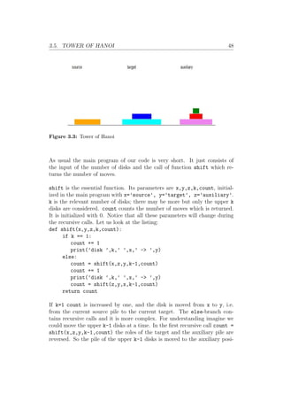
see figure 3.3. There are some legends about this game, see [42], [43].
We develop a short program with a recursive function which solves the game.
In the program part there is also the program Tower plot which uses turtle-
graphics. It demonstrates all the necessary moves, but the code is more
elaborate.](https://image.slidesharecdn.com/recursivealgorithmsr-250126092011-2b54067b/85/Recursive-Algorithms-coded-in-Python-pdf-48-320.jpg)
![3.6. THE KNAPSACK PROBLEM 49
tion. Then disk k moves to the target: print(’disk ’,k,’ ’,x,’-’,y).
The following call count = shift(z,y,x,k-1,count) means that the up-
per k-1 disks are moved from the auxiliary position to the target. But we
cannot move more than one disks at a time. So many recursive calls may be
necessary to move all disks to the target correctly. It can be shown that the
minimum number of necessary moves is 2n
−1 where n is the number of disks.
Let us look at an example. We set n = 3. ’source’, ’target’, ’auxiliary’
are abbreviated by s,t,a. In the main program shift(s,t,a,3,0) is called.
Then the following happens:
shift(s,t,a,3,0)
shift(s,a,t,2,0)
shift(s,t,a,1,0):count = 1; disk 1:s → t
count = 2; disk 2:s → a
shift(t,a,s,1,2):count = 3; disk 1:t → a
count = 4; disk 3:s → t
shift(a,t,s,2,4)
shift(a,s,t,1,4):count = 5; disk 1:a → s
count = 6; disk 2:a → t
shift(s,t,a,1,6):count = 7; disk 1:s → t
It should be mentioned that there exists an iterative solution of the game too,
see [44]. Anyhow the complexity of the algorithms (recursive or iterative) is
high. It can be shown that it is proportional to 2n
, see [45]. That’s why you
should not choose the number of disks greater than 6.
3.6 The Knapsack Problem
It is not difficult to explain what the knapsack problem is [46], [47]. Assume
there are several objects you want to put in your knapsack to transport them.
Every object has a known value and a known weight. The total weight of
objects carried in the knapsack may not exceed a certain limit maxweight.
Otherwise the knapsack would be damaged. But maxweight is smaller than
the sum of weights of all objects. So some of them must be left behind. The
problem is to find objects such that the sum of their values is maximal and
the sum of their weights is less or equal to maxweight. The set of objects
determined in this way is optimal to be transported in the knapsack.
The knapsack problem is interesting because it is an NP-problem [48], [49].
That means there is no known algorithm to solve it in polynomial time. How-](https://image.slidesharecdn.com/recursivealgorithmsr-250126092011-2b54067b/85/Recursive-Algorithms-coded-in-Python-pdf-50-320.jpg)
![3.6. THE KNAPSACK PROBLEM 50
ever, the knapsack problem can be solved using dynamic programming, see
[47]. This method works fine but it needs a lot of computer storage. Here
we prefer the method backtracking ([50], [51]) which needs no large storage.
We show how it works by a small example.
The weights and the values are given by the lists weight = [7,4,6,8,6]
and value = [4,4,5,4,6]. The limit of the weights is maxweight = 13.
The current optimal value is named optival, the corresponding numbers of
the objects (starting with 0) are stored in optiList. Initially optival = 0
and optiList = [] of course.
In the following scheme we show the way the optimal solution is found in the
example. Explanations see below.
[](0) → [0](4) → [0, 1](8) → [0, 1, 2](−)
↙
[0, 1](8) → [0, 1, 3](−)
↙
[0, 1](8) → [0, 1, 4](−)
↙
↙
[0](8) → [0, 2](9) → [0, 2, 3](−)
↙
[0, 2](9) → [0, 2, 4](−)
↙
↙
[0](9) → [0, 3](−)
↙
[0](9) → [0, 4](10)
↙
↙
[](10) → [1](10) → [1, 2](10) → [1, 2, 3](−)
↙
[1, 2](10) → [1, 2, 4](−)
↙
↙
[1](10) → [1, 3](10) → [1, 3, 4](−)
↙
↙
[1](10) → [1, 4](10)
↙
↙](https://image.slidesharecdn.com/recursivealgorithmsr-250126092011-2b54067b/85/Recursive-Algorithms-coded-in-Python-pdf-51-320.jpg)
 → [2](10) → [2, 3](−)
↙
[2](10) → [2, 4](11)
↙
[](11) → [3](11) → [3, 4](−)
↙
↙
[](11) → [4](11)
The currently chosen numbers of the objects are stored in indList. It is
part of list [0,1,2,3,4]. The number in parentheses is the current optimal
value optival. If there is a dash instead the corresponding indList is not
feasible, i.e. the sum of the associated weights exceeds maxweight. If an ar-
row points to the right the next possible number is added to indList. Then
the feasibility must be checked. Diagonal arrows stand for backtracking, and
the last number of indList is canceled.
The algorithm takes the first element of the list of weights and checks whether
or not maxweight is exceeded. It is not, thus optival is set to 4 and
indList = optiList = [0]. Also the sum of the first two weights is less
than maxweight. So optival = 8 and indList = optiList = [0,1]. How-
ever, the sum of the first three weights is greater than maxweight. indList =
[0,1,2], but optival and optiList remain unchanged, 2 must be removed
from indList. Next the algorithm tries to add 3 to indList, but [0,1,3]
is also infeasible etc.
The number of indlists which have to be checked is 23. Since there are
five objects there are 32 possibilities in total. But e.g. it is unnecessary to
check [0,1,2,3] because we already know that [0,1,2] is infeasible. The
reduction of the number of checks does not seem to be very large in our
example. But try the example in the exercises with eleven objects.
To code this method in Python we need some more variables. valList
and wtList are lists that contain values and weights. But they are not the
same as value and weight. valList is the list of values of the objects
of indList. wtList is defined analogously. For example: If indList =
[0,2,4], valList = [4,5,6] and wtList = [7,6,6] in the above exam-
ple. marked is a list of boolean variables which are initially all set False.
marked[index] is turned to True if it is impossible that a new and better
optival could be obtained by an indList containing index. We will discuss
this later in detail. n is just the number of objects, and count counts the
indLists to be considered. It is not necessary for the algorithm however.](https://image.slidesharecdn.com/recursivealgorithmsr-250126092011-2b54067b/85/Recursive-Algorithms-coded-in-Python-pdf-52-320.jpg)
![3.6. THE KNAPSACK PROBLEM 52
base on the other hand is very important. It tells the essential function
search which number to begin with if indList is temporarily empty. You
can see that this may happen when you look at the scheme above.
All lists except marked are initialized with [] and all numbers are initialized
with 0. Besides these settings the main program only consists of the call of
function search and the display of the results. This is the listing:
n = len(weight)
indList, optiList, valList, wtList = [], [], [], []
marked = [False for i in range(n)]
base, count, optival = 0, 0, 0
search(-1)
print(); print(’optimal value: ’,optival)
print(’optimal objects: ’,optiList)
print(’number of checks: ’,count)
The recursive function search does the essential work in this program. First
variables count, base, optival, optiList are declared global. What
does this mean, and why is this necessary? Normally all variables in Python
are local. That means they are only defined in the function where they occur.
But variables are global if they are defined in the main program (not in any
function). They may be used in functions as well. But we want to change
the values of the variables mentioned above inside the function. In this case
we have to declare them global. This keyword is not needed für printing
and accessing.
Then the auxiliary function find is called: y=find(current). This function
returns the first index not marked or -1 if there is no such index from the
argument current+1 on. When the program starts current = 0, no index
is marked, so find returns 0. However, later y will be set to -1. In that case,
backtracking is necessary.
But let’s consider the case if y = 0 first. current is set to y, and this value
is appended to indList, wtList and valList. This does not yet imply that
we found a new solution of our problem. The constraint sum(wtList) =
maxweight and the condition sum(valList) optival must be checked. If
both conditions are fulfilled, a new and better solution was found:
if (sum(wtList) = maxweight) (sum(valList) optival):
optival = sum(valList); optiList = indList.copy()
To avoid unnecessary searching the following two lines are important:
if sum(wtList) maxweight:
for ii in range(current+1,n):marked[ii] = True](https://image.slidesharecdn.com/recursivealgorithmsr-250126092011-2b54067b/85/Recursive-Algorithms-coded-in-Python-pdf-53-320.jpg)
![3.6. THE KNAPSACK PROBLEM 53
Consider indList=[0,1,2] in the scheme above. Then sum(wtList) =
7+4+6 = 17 maxweight. Consequently indices 3 and 4 are marked, and
indLists [0,1,2,3] , [0,1,2,4] and [0,1,2,3,4] are not checked. The
last line of the if-branch is the recursive call search(current) without any
terminal condition.
Now let us look at the else-branch. It is processed if y=-1, i.e. all fur-
ther indices are marked or there is none. Then backtracking has to be per-
formed. Thus current must be marked: marked[current] = True. clean
is an auxiliary function called with parameter indList[-1], the last item of
indList. All markers from indList[-1]+1 on are set to False. Why is this
necessary? Look at our example again. indList=[2,3] is infeasible because
weight[2]+weight[3]=6+8maxweight. So 3 and 4 are marked. But still
indList=[2,4] has not been checked, so 4 must be unmarked again. In
fact indList=[2,4] yields the optimal solution, and we don’t want to miss
it. Then the last items of indList, wtList and valList are removed. If
indList is not empty, current is assigned to the new last item of indList:
if indList != []:current = indList[-1].
For an empty indList things are more complicated. In this case current
must be set to base. Remember that base was set to 0 in the main program.
You can see from the scheme above that indList is empty for the first time
if all possibilities for 0 in indList are depleted. Therefore base must be
increased, and the next series starts with indList = [1]; no 0 occurs any-
more. Finally the recursive call follows including the terminal condition: if
basen:search(current). Here is the whole listing of search:
def search(current):
global count, base, optival, optiList
y = find(current)
if y = 0:
count += 1; current = y
indList.append(current)
wtList.append(weight[current])
valList.append(value[current])
if (sum(wtList)=maxweight) (sum(valList)optival):
optival = sum(valList); optiList = indList.copy()
if sum(wtList) maxweight:
for ii in range(current+1,n):marked[ii] = True
print(’count = ’,count,)
print(’optival = ’,optival,’ indList = ’,indList)
search(current)](https://image.slidesharecdn.com/recursivealgorithmsr-250126092011-2b54067b/85/Recursive-Algorithms-coded-in-Python-pdf-54-320.jpg)
![3.7. ILP WITH BRANCH AND BOUND 54
else: # backtracking
marked[current] = True
clean(indList[-1])
indList.pop(-1); wtList.pop(-1); valList.pop(-1)
if indList != []:current = indList[-1]
else:
current = base; base += 1
if base n: search(current)
Finally we denote the listings of the small auxiliary functions:
def find(x):
posi = -1
for j in range(n-1,x,-1):
if (not marked[j]): posi = j
return posi
def clean(x):
y = x + 1
while y = n-1:
marked[y] = False; y += 1
3.7 ILP with Branch and Bound
ILP stands for Integer Linear Program. This is a linear optimization prob-
lem [52] in which only integer solutions are to be determined. Such problems
are important because often only integer solutions make sense. For example
you can’t buy 4.73 cars, and only integer numbers of sofas can be produced.
It is not possible just to solve a linear optimization problem with real solu-
tions and then obtain the solution for your ILP by rounding. The reason is
that rounded solutions may be infeasible.
There are several methods for finding optimal solutions of a general lin-
ear optimization problem. A well-known method is the simplex method, see
[53], [54]. This method usually works very well, but it can only be shown
that it has exponential runtime. But in fact such problems can be solved in
polynomial time (see [55]). This means that there exists an integer k such
that the running time is limited by nk
where n is the number of variables.
There is an efficient scipy function for solving general linear problems. So
we shall concentrate on solving integer linear problems.](https://image.slidesharecdn.com/recursivealgorithmsr-250126092011-2b54067b/85/Recursive-Algorithms-coded-in-Python-pdf-55-320.jpg)
![3.7. ILP WITH BRANCH AND BOUND 55
One strategy to solve them is Branch and Bound. Generally this is a tem-
plate for certain algorithms. The problem is split into two or more problems
which can be solved easier than the original one. In most cases this results
in a tree. Bounding means that some branches may be canceled because of
constraints included in the original problem.
Especially it is useful for integer optimization problems. One might think
that finding only integer solutions is easier than solving the corresponding
problem for real solutions. But the opposite is correct. No algorithm is
known that solves ILPs in polynomial time. Applying Branch and Bound
may be helpful by reducing the number of branches to be checked.
The first step consists in a relaxation. The constraint that only integer so-
lutions are to be determined is omitted. The obtained optimal solution may
contain non integer values, for example x3 = 1.5. Then the original problem
is split into two new problems. The first one is the original problem with the
additional constraint x3 ≤ 1 and the second is the original problem with the
additional constraint x3 ≥ 2. When the first problem is solved it may hap-
pen that x4 = 7.3. In this case another branching has to be performed. The
branching is repeated until one of the following cases occurs: (1) An integer
solution was found. (2) The current linear problem is infeasible. (3) A better
solution has already been obtained. The next step consists in collecting all
integer solutions, and finally the best of these is selected.
Now we will code an ILP in Python. In order to explain how the program
works we use an example found in a text from the university of Siegen (Ger-
many) [56]. The advantage is that this example is not very complicated but
on the other hand it is not trivial. Here it is:
The objective function to be minimized is given by c(x) := −x1 − x2.
The constraints are
− 2x1 + x2 ≤ −
1
2
− x2 ≤ −
1
2
2x1 + x2 ≤
11
2
First the required data must be available for processing, i.e. the objective
function and the constraints. It is rather tough to type all the needed data](https://image.slidesharecdn.com/recursivealgorithmsr-250126092011-2b54067b/85/Recursive-Algorithms-coded-in-Python-pdf-56-320.jpg)

![3.7. ILP WITH BRANCH AND BOUND 57
optimization yields at least one variable which is not integer. It returns a
boolean variable which has the value True if a solution of the ILP was found.
The parameters are ind, x, A, B, xList, yList. ind is the first index
of a non-integer variable. x is the current list of variables, A is the current
matrix, and B is the current vector of the right hand side. We emphasize
the word ’current’ because the values of these variables will probably change
during recursive calls of branch. xList is the list of all lists of variables,
and yList is the list of the corresponding optimal values obtained during
preceding optimizations.
branch initializes the local variables found l and found r with False. They
will turn to True as soon as an integer solution is found in the left or right
branch. The line xl,yl,Al,Bl,succ = left(ind,x,A,B) follows. Function
left adds one more constraint to the current system. The new constraint
consists of a 1 inserted at the position of index ind. All other coefficients on
the left hand side are set to 0. So a new row A is added to matrix A, the
resulting matrix is A0. Vector B is supplemented by = ⌊x[ind]⌋, resulting in
B0. Then the new LP is solved by calling solve LP with parameters obj, the
objective function, and A0 and B0; these are the new built matrix of coeffi-
cients and the vector on the right hand side. If the solution is not feasible
(that means succ == False) y0 is set to np.inf, that is infinity. So it is
ensured that this is certainly not the optimal solution of the problem. left
returns the new optimal variables of the LP x0, the new optimal solution y0
and the expanded matrix A0, vector B0 and finally succ to decide whether
or not the solution of the linear problem was successful.
The function right works in a quite similar way. We have just to re-
member that the new constraint x[ind] ≥ ⌈b[ind]⌉ has to be replaced by
−x[ind] ≤ −⌈b[ind]⌉. So we have to set A [ind] = -1; A1 = A + [A ].
The vector B must be supplemented by B1 = B + [-np.ceil(x[ind])].
Now let’s return to function branch. If an integer and feasible solution was
found the obtained new list xl and the corresponding optimal value yl are
appended to the lists xList and yList respectively. found l is then set to
True. This is coded in these three lines:
if allInt(xl) (yl != np.inf):
xList.append(xl); yList.append(yl)
found l = True
This was outlined for the left branch. The corresponding part for the right
branch looks quite analogously.](https://image.slidesharecdn.com/recursivealgorithmsr-250126092011-2b54067b/85/Recursive-Algorithms-coded-in-Python-pdf-58-320.jpg)
![3.7. ILP WITH BRANCH AND BOUND 58
However, in most cases we shall not obtain integer solutions, and branch-
ing must go on. Whenever we have obtained a non-integer variable by the
functions left and right we could perform another branching. This is done
in the Python script IPL 2. It is obvious that the computing effort grows
exponentially with the number of non-integer variables. But we can reduce
the number of branches by bounding.
We return to the example from above to explain the idea. The LP relaxation
yields the optimal value y = −4 where x1 = 1.5, x2 = 2.5. So branching has
to be performed. The additional constraints are x1 ≤ 1 for the left branch
and x1 ≥ 2 for the right one. Function left yields yl = -2.5 and xl = [1,
1.5], whereas function right gives yr = -3.5 and xr = [2, 1.5]. The
minimum of yl and yr is a bound to the optimal value of the ILP. It cannot
be smaller than -3.5. Since yr is less than yl we shall first try to find an
integer solution using the right branch. If we obtain such a solution with an
optimal value −2.5 it is not necessary to consider the left branch. Only
if the right branch yields no feasible integer solution it is necessary to try to
get a solution from the left branch.
In our example the right branch seems to be the better choice, and we haven’t
got an integer solution yet. Thus the following part of function branch will
be executed:
if (yr = bound) (yr != np.inf) (found r == False):
i = 0
while (i len(xr)-1) isInt(xr[i]) :i += 1
if i len(xr):found r=branch(i,xr,Ar,Br,xList,yList)
We see that all the conditions of the if-clause are fulfilled. The next two
lines detect the first index i where the variable x[i] has no integer value, if
there is any. If such an index is found finally the recursive call of function
branch is executed. The corresponding part for the left branch looks quite
the same and need not be discussed here.
Our example now gives yl = -3.25 and xl = [2.25, 1]. The right branch
yields yr = -4 and xr = [2, 2]. But this solution is not feasible (the third
constraint is not fulfilled), and it has to be canceled.
One more branching is necessary to obtain yl=-3, xl = [2,1] and yr=-3.5,
xl = [3,0.5]. The latter solution is not feasible, so the optimal value is
y = −3 with x1 = 2, x2 = 1. Since this optimal value is smaller than the
former received left branch value −2.5 we need not consider the left branch
of the first branching. The complete solution is shown in the sketch below.](https://image.slidesharecdn.com/recursivealgorithmsr-250126092011-2b54067b/85/Recursive-Algorithms-coded-in-Python-pdf-59-320.jpg)
![3.7. ILP WITH BRANCH AND BOUND 59
yl = −4, xl = [1.5, 2.5]
/
left x1 = 1 right x1 = 2
yl = −2.5, xl = [1, 1.5] yr = −3.5, xr = [2, 1.5]
/
left x2 = 1 right x2 = 2
yl = −3.25, xl = [2.25, 1] yr = −4, infeasible
/
left x1 = 2 right x1 = 3
yl = −3
yl = −3
yl = −3, xl = [2, 1]
xl = [2, 1]
xl = [2, 1] yr = −3, 5, infeasible
Example for an ILP The complete tree according to our example; there is
no need to pursue the upper left branch because the optimal objective value
is −3 which is less than yl in the upper left branch.
Function branch is nearly complete, but there is still one case left. It is
possible that the putative better branch (with the lower value of the objec-
tive function) gives no feasible solution. Then the remaining branch has to
be considered.
y2 = np.inf; found2 = False
if yl bound: y2 = yl; x2 = xl; A2 = Al; B2 = Bl
if yr bound: y2 = yr; x2 = xr; A2 = Ar; B2 = Br
The preceding three lines effect that parameters of the remaining branch
are assigned index 2. So we need only one more function call for branching.
We also have to keep in mind that this call is only necessary if no integer
solution has been found yet and if y2 is greater than bound. The interior of
the if-clause is quite analogous to the cases treated before.
if (y2 != np.inf)(found l == False)(found r == False):
i = 0
while (i len(x2)-1) isInt(x2[i]) :i += 1
if i len(x2):found2 = branch(i,x2,A2,B2,xList,yList)
There are three possibilities to find an integer solution during the course
of function branch: find l or find r may turn to True, and finally find2
may become True. Therefore the last line of the function is
return found l or found r or found2.
Here is the listing of function branch:](https://image.slidesharecdn.com/recursivealgorithmsr-250126092011-2b54067b/85/Recursive-Algorithms-coded-in-Python-pdf-60-320.jpg)
![3.7. ILP WITH BRANCH AND BOUND 60
def branch(ind,x,A,B,xList,yList):
found l = False; found r = False
xl,yl,Al,Bl,succ = left(ind,x,A,B)
if succ:
if allInt(xl) (yl != np.inf):
xList.append(xl); yList.append(yl)
found l = True
xr,yr,Ar,Br,succ = right(ind,x,A,B)
if succ:
if allInt(xr) (yr != np.inf):
xList.append(xr); yList.append(yr)
found r = True
bound = min(yl,yr)
if (yl = bound)(yl != np.inf)(found l == False):
i = 0
while (i len(xl)-1) isInt(xl[i]) :i += 1
if ilen(xl):found l = branch(i,xl,Al,Bl,xList,yList)
if (yr = bound)(yr != np.inf)(found r == False):
i = 0
while (i len(xr)-1) isInt(xr[i]) :i += 1
if ilen(xr):found r = branch(i,xr,Ar,Br,xList,yList)
y2 = np.inf; found2 = False
if yl bound:y2 = yl; x2 = xl; A2 = Al; B2 = Bl
if yr bound:y2 = yr; x2 = xr; A2 = Ar; B2 = Br
if (y2 != np.inf)(found l == False)(found r == False):
i = 0
while (i len(x2)-1) isInt(x2[i]) : i += 1
if ilen(x2):found2 = branch(i,x2,A2,B2,xList,yList)
return found l or found r or found2
The main program is not so exciting. It starts with some initialization:
epsilon = 1e-6, xList and yList are set to []. A text file (see above)
is read to obtain the objective function as well as the constraints. The LP
is solved: x,y, succ = solve LP(obj,A,B). If the solution of the LP is al-
ready integer or if it is infeasible the result is displayed. Otherwise branching
begins. In the end xList, yList and the result are displayed.
The program part contains three versions: ILP only displays the results
whereas ILP 3 also shows a lot of intermediate results so you can see how it](https://image.slidesharecdn.com/recursivealgorithmsr-250126092011-2b54067b/85/Recursive-Algorithms-coded-in-Python-pdf-61-320.jpg)
![3.8. EXERCISES 61
works. There is also a version ILP 2 where only branching is implemented
but no bounding. The runtime difference between the latter two versions
may seem unimportant, but take notice of exercise 6.
3.8 Exercises
Figure 3.4: Curve of hooks and snowflake curve
1. Curve of Hooks [57] and Snowflake Curve [58]
Develop programs for drawing these curves. Step one of them is de-
picted in figure 3.4. The recursive function draw belonging to the curve
of hooks starts with width = width // 4. For the snowflake curve
it is sufficient to divide width by 3. If step == 0 the recursive call
draw(width,step-1) simply means tu.forward(width).
The main program is the same for both curves. Here it is:
for count in range(3):
tu.up(); tu.setpos(-300,0); tu.down()
tu.width(2)
draw(800,count)
time.sleep(3)
tu.clearscreen()
tu.up(); tu.hideturtle()
tu.setpos(-300,-250)
tu.pencolor((0,0,0))
tu.write(’finished!’,font = (Arial,12,normal))
tu.exitonclick() # für PyCharm
try:tu.bye()
except tu.Terminator:pass
Hint: Do not forget to import time at the beginning of the programs.
2. Fibonacci Function of higher Order
The Fibonacci function fibop of order p of a number n is defined by](https://image.slidesharecdn.com/recursivealgorithmsr-250126092011-2b54067b/85/Recursive-Algorithms-coded-in-Python-pdf-62-320.jpg)
![3.8. EXERCISES 62
the sum of the p + 1 predecessors of n [59]. If n = p, fibop(p) = 1, if
n p : fibop(n) = 0.
Write a program for computing values of fibop applying a recursive or
an iterative algorithm. The user may decide the kind of algorithm.
3. Q function
The Q function invented by D. R. Hofstadter [60] is defined thus:
Q(k) =
1, if k ≤ 2
Q(k − Q(k − 1)) + Q(k − Q(k − 2)) otherwise
Write a program for computing values of this function applying a re-
cursive or an iterative algorithm. The user may decide the kind of
algorithm.
Remark: It has not been proven that the Q function is well-defined.
Possibly the recursion demands negative arguments for which Q does
not exist. But this is unlikely [60], [61].
4. Permutations
The following code corresponds to Heap’s algorithm for computing
permutations [62], [63]. Perform a desk test for this code for m=3, A
= [1,2,3] and denote in which order the permutations are displayed.
def Perm(m):
if m == 1:
print(A)
for i in range(m):
Perm(m-1)
if m % 2 == 1:
A[m-1], A[0] = A[0], A[m-1]
else:
A[m-1], A[i] = A[i], A[m-1]
5. Knapsack Problem
(i) Run program ”Knapsack backtracking” with weight = [6,8,7], value
= [5,6,8] and maxweight = 13.
(ii) Run it with weight = [5, 7, 6, 8, 10, 11, 12, 15, 17, 30, 18] , value
= [8, 9, 6, 5, 10, 5, 10, 17, 19, 20, 13] and maxweight = 33.
(iii) Alter the program such that it checks all possibilities for arranging
the set of objects.
6. ILP
(1) Test all text files using program versions ILP 3 and ILP 2.](https://image.slidesharecdn.com/recursivealgorithmsr-250126092011-2b54067b/85/Recursive-Algorithms-coded-in-Python-pdf-63-320.jpg)
![3.8. EXERCISES 63
(2) Find examples for every case that can occur and test your examples:
(i) the LP is infeasible,
(ii) the LP relaxation yields an integer solution,
(iii) the LP is feasible but the ILP is not.
(3) Solve the following ILP (adapted from [64]) .
max −2x1 + x2 − 8x3
subject to:
2x1 − 4x2 + 6x3 ≤ 3
−x1 + 3x2 + 4x3 ≤ 2
2x3 ≤ 1
x1, x2, x3 ≥ 0
Use programs ILP 3 and ILP 2. Count the different number of calls of
function branch. Do you think that it is worthwhile to use bounding?](https://image.slidesharecdn.com/recursivealgorithmsr-250126092011-2b54067b/85/Recursive-Algorithms-coded-in-Python-pdf-64-320.jpg)
![64
Chapter 4
Some Indirect Recursive
Algorithms
4.1 Collatz Conjecture
The problem is quite simple to formulate: Consider an integer number 0.
If it is odd, multiply by three and add one. If it is even, divide it by two.
Before 1950 Collatz stated that each sequence of positive integers built
according to these two rules ends with ...4,2,1,4,2,1,... [65], [66]. This is the
Collatz conjecture. An example is 17 → 52 → 26 → 13 → 40 → 20 → 10 →
5 → 16 → 8 → 4 → 2 → 1 → 4 → 2 → 1 ...
In recent years many mathematicians tried to prove the Collatz conjecture
[67]. But no one could prove it. If you find a proof, you’ll win a prize [68].
We will not try to prove it. Instead we shall develop a simple example for two
functions which call each other recursively. The program will not continue
indefinitely with 4,2,1, it will end as soon as number 1 is reached. Here is
function even:
def even(n):
print(n,end = ’ ’)
n = n //2
if n % 2 == 0:even(n)
else:odd(n)
After having displayed the current number n it is divided by two using integer
division, i.e. n // 2. The term n % 2 checks whether n is even or odd. If it
is even, n % 2 = 0 otherwise it is 1. A termination condition is not needed
in this function because the sequence does not end with an even number.](https://image.slidesharecdn.com/recursivealgorithmsr-250126092011-2b54067b/85/Recursive-Algorithms-coded-in-Python-pdf-65-320.jpg)
![4.2. MONDRIAN 65
Function odd looks similarly simple:
def odd(n):
if n == 1:print(1)
else:
print(n,end = ’ ’)
even(3*n+1)
Here a termination condition is present: if n == 1:print(1). Otherwise
a recursive call of even follows the display of n. The main program is very
short. The user is asked to enter an odd number. Then function odd is
called. This way we obtain two functions that call each other recursively.
Since even is not called from the main program it is an indirect recursion.
Only one of the functions needs a termination condition, but it is also possi-
ble to implement such a condition in each of the two functions.
What makes the Collatz conjecture interesting is among other aspects that
the sequences arising from odd numbers have very different lengths. Try
27, 97, 113, 491, 497 and 9663. The lengths of the sequences have evidently
nothing to do with prime numbers. Some sequences grow to enormous values
but finally they all reach 4,2,1. For example the maximum of the sequence
starting with 27 is 9232, and starting with 9663 you will reach 27,114,424.
4.2 Mondrian
Piet Mondrian (1872 - 1944) was a famous Dutch painter [69], [70]. Many
museums especially in the Netherlands exhibit his paintings [71]. Works be-
longing to the artistic movement ”new plasticism” are often composed of
black horizontal and vertical bars which form a grid pattern. Some of the
rectangular areas of the grid are filled with intensive colors red, blue and
yellow [72], [73].
We want to develop a program which produces images modeled after this kind
of paintings. Of course their quality is not comparable to original works. It
is easy to see that the balance is missing. One reason is the use of random
numbers in the program. We shall just apply the technique of the kind of
paintings described above. A possible result is shown in Figure 4.2.
The essential functions are horizontal and vertical. They are mutually
recursive, i.e. vertical calls horizontal and horizontal calls vertical
until a terminal condition has been reached. Both functions need four pa-](https://image.slidesharecdn.com/recursivealgorithmsr-250126092011-2b54067b/85/Recursive-Algorithms-coded-in-Python-pdf-66-320.jpg)


![4.3. SHAKERSORT 69
4.3 Shakersort
Bubblesort is a sorting method which is easy to understand, but it works very
slowly. A similar method is Shakersort [74], and we may suppose that it works
faster. The idea is the following: As in Bubblesort [75] the algorithm steps
through the elements starting with the last, compares the current element
with its predecessor and swaps them if they are in wrong order, see left
column of the scheme below. However, when the first run is finished and
the element with the smallest key is at position 1, the direction of sorting is
reversed, and it starts at position 2, see the middle column of the scheme. So
it is ensured that an element with the largest key stands at the last position.
Then the direction of sorting is reversed again, and it starts at the last
position but one, see right column of the scheme. Changing the directions
and swapping continue until the whole sorting is done. In our example just 8
characters will be sorted alphabetically. In this example sorting is completed
after two backward runs and one forward run. But in general more runs are
necessary.
sorting backward sorting forward sorting backward
E C B F A H G D
E C B F A H D G A E C B F D H G A C B E D F G H
E C B F A D H G A C E B F D H G A C B E D F G H
E C B F A D H G A C B E F D H G A C B E D F G H
E C B A F D H G A C B E F D H G A C B D E F G H
E C A B F D H G A C B E D F H G A C B D E F G H
E A C B F D H G A C B E D F H G A B C D E F G H
A E C B F D H G A C B E D F G H
We demonstrate this sorting method similarly to mergesort, see section 3.4.
To do that we choose 60 capital letters randomly. This is done in the main
program. The list a is initialized by [].
for i in range(n):# set n = 60
a.append(rd.randint(65, 90))
update(a,i)
The letters are to be sorted alphabetically. Whenever a letter is moved,
more exactly: swapped with one of its neighbors, function update is called.
We will not discuss this function in detail. update(a,kk) moves the turtle to](https://image.slidesharecdn.com/recursivealgorithmsr-250126092011-2b54067b/85/Recursive-Algorithms-coded-in-Python-pdf-70-320.jpg)
![4.3. SHAKERSORT 70
the correct position. Any character that may be at that position is deleted.
Then the turtle writes a[kk].
The essential functions are back and forward. They need three parame-
ters: the list a, and l and r which mark the left and right border of the
region where sorting has still to be done. At the beginning, l = 0 and r =
n-1; remember that Python starts counting at 0. If there are 60 letters to
sort their positions are numbered 0, ..., 59. Function shakersort itself just
consists of the call back(0,n-1).
Functions back and forward look very similar, but there are some impor-
tant differences. We will discuss back first. The introduced variable k will
mark the next left border. Initially it is set to r, and it remains r, if the
list is already sorted. The following for-loop starts at r and ends at l. The
third parameter of range is -1, and that means that j counts backwards, for
example 8,7,6,...,0. If an element with a greater key stands just left of the
current element, they are swapped and updated. In this case, k is set to j be-
cause the element swapped to the right must possibly be swapped again. So
we are not sure that sorting is already done from position j on. Finally the
indirect recursive call follows: if k r:forward(a,k,r). Forward sorting
makes sense only if k r. Otherwise the list is already sorted. Here is the
listing of back:
def back(a,l,r):
k = r
for j in range(r,l,-1):
if a[j-1] a[j]:
a[j], a[j-1] = a[j-1], a[j]
update(a,j-1); update(a,j)
k = j
if k r: forward(a,k,r)
In forward k is initially set to 0. If the list is already sorted, k does not
change. The following for-loop counts in forward direction. Notice that the
right bound is r+1. Why is this necessary? Possibly a[r] and a[r-1] must
be swapped. So index r must be reached by the loop. But the last index is
only r-1 in range(l,r), a special feature of Python. The last line contains
the recursive call: if l k:back(a,l,k). The case l = k would show
that sorting is already done. This is the whole listing:
def forward(a,l,r):
k = 0
for j in range(l,r+1):
if a[j-1] a[j]:
a[j], a[j-1] = a[j-1], a[j]](https://image.slidesharecdn.com/recursivealgorithmsr-250126092011-2b54067b/85/Recursive-Algorithms-coded-in-Python-pdf-71-320.jpg)
![4.4. SIERPINSKI CURVES 71
update(a,j-1); update(a,j)
k = j
if l k: back(a,l,k)
Is Shakersort significantly better than Bubblesort? We made a small experi-
ment to explore this. With n = 60 and tu.speed(6) we ran Shakersort and
Bubblesort ten times each. The mean value of the time consumed was 113.5
± 14.5 s for Shakersort and 119.5 ± 10.7 s for Bubblesort. From that we can
see that Shakersort was slightly better than Bubblesort but not significantly.
It can be shown that the time complexity of both methods is O(n2
), see [74].
If the number of elements is multiplied by 2, 3 etc. the time consumption
must be multiplied by 4, 9 etc. Therefore Shakersort is not recommended for
sorting large numbers of elements. But the method is funny, isn’t it?
4.4 Sierpinski Curves
In 1912 the Polish mathematician Waclaw Sierpiński developed the se-
quence of fractal curves [76] we want to code. The curves of the sequence
are closed, and they all lie inside a finite area, e.g. the unit square. But
their lengths grow exponentially with the number of step n. The limit for
n → ∞ is a curve which runs through every point of an area; it is called
”space-filling”.
A Sierpiński curve [77] [78] consists of bulges and passages. If n=1, a passage
is just a line of length h2; one of four bulges is colored red in figure 4.3.
In function bulge we have to treat the basic case step = 1 and the re-
cursive case step 1 differently. The basic case explains itself. Evidently
passing a bulge turns the turtle to the right by 90°.
if step == 1:
tu.left(45);tu.forward(h2)
tu.right(90);tu.forward(h2)
tu.right(90);tu.forward(h2)
tu.left(45)
From figure 4.4a it can be seen in which way the code for a bulge has to be
replaced for step 1. It is not sufficient just to substitute a simple bulge
by three smaller ones. Instead the turtle must turn by 45° to the left and
then move along a passage. Then it turns once more by 45° to the left and
moves forward. When this is finished three bulges are drawn each of them
followed by a forward move. At last passage is called again, framed by two
more turns by 45° to the left. This is the else-branch:](https://image.slidesharecdn.com/recursivealgorithmsr-250126092011-2b54067b/85/Recursive-Algorithms-coded-in-Python-pdf-72-320.jpg)


![4.5. EXERCISES 74
n=int(input(’n = (1,...,6) ’))
h0=200
for i in range(n):
h0=h0*(4+math.sqrt(2))/(8+3*math.sqrt(2))
h=round(h0);h2=round(math.sqrt(2)*h0)
tu.width(2);tu.speed(5)
# move to the start position
tu.up();tu.setpos(-100,60);tu.down();tu.left(90)
for i in range(4):
bulge(h,h2,n);tu.forward(2*h)
# final part, see section 1.1.2
This was only one example for a sequence of curves with a space-filling limit.
Of course there are many more of them. Some are closed curves and some
are not. For more information about space-filling curves see [79]. It should
be possible to write a code using turtlegraphics to model Hilbert curves, see
[80]. More than two mutually recursive functions are necessary for modeling
these curves.
4.5 Exercises
1. Indirect Recursive Figures
(i) Write a program with two indirect recursive functions ”square” and
”triangle”. The result could look like figure 4.5a.
(ii) Write a program with two indirect recursive functions ”triangle”
and ”rectangle”. The result could look like figure 4.5b.
a b
Figure 4.5: (a) Functions square and triangle call each other. (b) Functions
triangle and rectagle call each other.](https://image.slidesharecdn.com/recursivealgorithmsr-250126092011-2b54067b/85/Recursive-Algorithms-coded-in-Python-pdf-75-320.jpg)

![76
Appendix
How to terminate Turtlegraphics
Though it is really fun to deal with turtlegraphics there is a general problem.
Whenever a drawing with turtlegraphics is finished the following line of the
code is (see chapters 1 - 4):
tu.write(’finished!’,font = (Arial,12,normal)).
But how can you achieve that the panel for turtlegraphics is closed and the
program returns to the editor? There is no general answer to this question.
It depends on the operating system of the computer but also on the Python
editor. Two editors frequently used are PyCharm [4] and Spyder [5].
Things are quite simple with PyCharm. Simply add these lines following
the line with ”finished!”:
tu.exitonclick()
try:
tu.bye()
except tu.Terminator:
pass
This is already done in the listings of chapters 1 - 4. Then a mouse click on
the panel suffices. The panel is closed, and the program returns to the editor.
Things are not so simple with Spyder. In [81] the following two lines are
recommended:
turtle.done()
turtle.bye()
A mouse click on the panel won’t help. You must click on the cross for clos-
ing the panel. But what happens then cannot be predicted. There are three
possibilities:
(1) The panel is closed, and the program returns to the editor. That is the
best possible result.](https://image.slidesharecdn.com/recursivealgorithmsr-250126092011-2b54067b/85/Recursive-Algorithms-coded-in-Python-pdf-77-320.jpg)
![4.5. EXERCISES 77
(2) An error message is displayed similar to this one:
runfile(’D:/myPython/xyz.py’, wdir=’D:/myPython’)
Traceback (most recent call last):
File D:Anaconda3Libsite-packagesspyder kernelspy3compat.py:356
in compat exec
exec(code, globals, locals)
File d:mypythonxyz.py:25
tu.done()
File string:5 in mainloop
Terminator
Surely you are not happy about that message, but after all you are back to
the IPython console.
(3) An extremely long error message is displayed which is not cited in too
much detail. It starts with
Tcl AsyncDelete: async handler deleted by the wrong thread
Windows fatal exception: code 0x80000003
and ends with
Restarting kernel... .
According to [81] the error messages could be suppressed by using these lines:
tu.done()
try:
tu.bye()
except tu.Terminator:
pass
However, this is not always successful.
On the other hand sometimes the lines provided for PyCharm are also suc-
cessful with Spyder.
Link to Program Part
The complete Python scripts for Chapters 1 - 4 as well as the solutions to
the exercises can be found here:
https://drthpeters.github.io/Recursive-Algorithms-Python/](https://image.slidesharecdn.com/recursivealgorithmsr-250126092011-2b54067b/85/Recursive-Algorithms-coded-in-Python-pdf-78-320.jpg)
![78
References
[1] Python can be downloaded from https://www.python.org/downloads
[2] The concept of the programming language Logo is described in
https://el.media.mit.edu/logo-foundation/what_is_logo/logo_
primer.html
[3] https://docs.python.org/3/library/turtle.html
[4] https://www.jetbrains.com/de-de/pycharm/download/?section=
windows
[5] https://www.spyder-ide.org/download/
[6] https://plato.stanford.edu/entries/nicole-oresme/
[7] https://www.cantorsparadise.com/the-euler-mascheroni-constant-4bd34203aa01
[8] https://www.olabs.edu.in/?sub=97brch=48sim=492cnt=1
[9] https://en.wikipedia.org/wiki/Euclidean_algorithm
[10] https://socratic.org/questions/what-does-the-alternating-harmonic-series-con
[11] https://www.britannica.com/topic/Pi-Recipes-1084437
[12] https://slideplayer.org/slide/2837657/
[13] https://realpython.com/fibonacci-sequence-python/
[14] https://en.wikipedia.org/wiki/Hero_of_Alexandria
[15] https://web2.0calc.com/questions/using-heron-s-method-what-is-the-square-roo
[16] https://en.wikipedia.org/wiki/Catalan_number
[17] https://www.whitman.edu/mathematics/cgt_online/book/
section03.05.html](https://image.slidesharecdn.com/recursivealgorithmsr-250126092011-2b54067b/85/Recursive-Algorithms-coded-in-Python-pdf-79-320.jpg)
![REFERENCES 79
[18] https://en.wikipedia.org/wiki/Noncrossing_partition
[19] https://en.wikipedia.org/wiki/Binomial_coefficient
[20] https://en.wikipedia.org/wiki/Binomial_distribution
[21] https://brilliant.org/wiki/binomial-coefficient/
[22] https://math.libretexts.org/Bookshelves/Linear_Algebra/A_
First_Course_in_Linear_Algebra_(Kuttler)/03%3A_Determinants/
3.02%3A_Properties_of_Determinants
[23] https://en.wikipedia.org/wiki/Determinant
[24] https://en.wikipedia.org/wiki/Parallelepiped
[25] https://www.purplemath.com/modules/cramers.htm
[26] https://en.wikipedia.org/wiki/Computational_complexity_of_
mathematical_operations
[27] https://en.wikipedia.org/wiki/Abel%E2%80%93Ruffini_theorem
[28] https://en.wikipedia.org/wiki/Cubic_equation
[29] https://en.wikipedia.org/wiki/Quartic_function
[30] https://www.tandfonline.com/doi/full/10.1080/23311835.2016.
1277463
[31] https://en.wikipedia.org/wiki/Horner%27s_method
[32] https://en.wikipedia.org/wiki/Pascal%27s_triangle
[33] https://en.wikipedia.org/wiki/Regula_falsi
[34] https://en.wikipedia.org/wiki/Gaussian_elimination
[35] https://en.wikipedia.org/wiki/Dragon_curve The dragon curves
shown on this Site are similar but not quite the same as in sec. 3.1.
[36] http://aleph0.clarku.edu/~djoyce/ma114/comb.pdf
[37] https://en.wikipedia.org/wiki/Ackermann_function
[38] https://en.wikipedia.org/wiki/Primitive_recursive_function](https://image.slidesharecdn.com/recursivealgorithmsr-250126092011-2b54067b/85/Recursive-Algorithms-coded-in-Python-pdf-80-320.jpg)
![REFERENCES 80
[39] https://training.incf.org/sites/default/files/2019-02/03_
lester_.pdf
[40] https://www.tcs.ifi.lmu.de/lehre/ss-2024/fsk_de/
vl-09c-f-die-ackermannfunktion.pdf
[41] https://www.tutorialspoint.com/data_structures_algorithms/
merge_sort_algorithm.htm
[42] https://www.vanishingincmagic.com/puzzles-and-brainteasers/
articles/history-of-tower-of-hanoi-problem/
[43] https://www.scientificamerican.com/article/
the-tower-of-hanoi/#:~:text=The%20tower%20of%20Hanoi%
20(also,mental%20discipline%20of%20young%20priests.
[44] https://www.geeksforgeeks.org/iterative-tower-of-hanoi/
[45] https://www.baeldung.com/cs/towers-of-hanoi-complexity
[46] https://en.wikipedia.org/wiki/Knapsack_problem
[47] https://www.educative.io/blog/0-1-knapsack-problem-dynamic-solution
[48] https://mathworld.wolfram.com/NP-Problem.html
[49] https://deepai.org/machine-learning-glossary-and-terms/
nondeterministic-polynomial-time
[50] https://en.wikipedia.org/wiki/Backtracking
[51] https://www.programiz.com/dsa/backtracking-algorithm
[52] https://www.cimt.org.uk/projects/mepres/alevel/discrete_
ch5.pdf
[53] http://www.phpsimplex.com/en/simplex_method_example.htm
[54] https://users.mai.liu.se/torla64/MAI0130/Beatrice%202pre.
pdf
[55] http://public.tepper.cmu.edu/jnh/karmarkar.pdf
[56] from OPTI2.dvi(uni-siegen.de), unfortunately no longer available
[57] https://en.wikipedia.org/wiki/Z-order_curve The curve of hooks
is similar to the Lebesgue curve or Z curve.](https://image.slidesharecdn.com/recursivealgorithmsr-250126092011-2b54067b/85/Recursive-Algorithms-coded-in-Python-pdf-81-320.jpg)
![REFERENCES 81
[58] https://larryriddle.agnesscott.org/ifs/kcurve/kcurve.htm
[59] http://www.modernscientificpress.com/
Journals/ViewArticle.aspx?XBq7Uu+HD/
8eRjFUGMqlRSziRNLeU2RixB4ndiJghEnTfTElvDRYUuwGofG1d+5T
[60] https://en.wikipedia.org/wiki/Hofstadter_sequence
[61] https://cs.uwaterloo.ca/journals/JIS/VOL9/Emerson/emerson6.
pdf
[62] https://en.wikipedia.org/wiki/Heap%27s_algorithm
[63] https://www.geeksforgeeks.org/heaps-algorithm-for-generating-permutations/
[64] https://www.uni-muenster.de/AMM/num/Vorlesungen/maurer/
Uebungen09.pdf
[65] https://en.wikipedia.org/wiki/Collatz_conjecture
[66] https://www.quantamagazine.org/why-mathematicians-still-cant-solve-the-colla
[67] https://www.quantamagazine.org/mathematician-proves-huge-result-on-dangerous
Don’t miss the video!
[68] https://mathprize.net/posts/collatz-conjecture/
[69] https://en.wikipedia.org/wiki/Piet_Mondrian
[70] https://blog.artsper.com/en/a-closer-look/
10-things-to-know-about-piet-mondrian/
[71] https://www.holland.com/global/tourism/search.htm?keyword=
Mondrian
[72] https://en.wikipedia.org/wiki/Piet_Mondrian#/media/File:
Tableau_I,_by_Piet_Mondriaan.jpg
[73] https://en.wikipedia.org/wiki/Piet_Mondrian#/media/File:
Piet_Mondriaan,_1939-1942_-_Composition_10.jpg
[74] https://en.wikipedia.org/wiki/Cocktail_shaker_sort
[75] https://en.wikipedia.org/wiki/Bubble_sort
[76] https://medical-dictionary.thefreedictionary.com/Fractal+
curve](https://image.slidesharecdn.com/recursivealgorithmsr-250126092011-2b54067b/85/Recursive-Algorithms-coded-in-Python-pdf-82-320.jpg)
![REFERENCES 82
[77] https://en.wikipedia.org/wiki/Wac%C5%82aw_Sierpi%C5%84ski
[78] https://en.wikipedia.org/wiki/Sierpi%C5%84ski_curve
[79] https://en.wikipedia.org/wiki/Space-filling_curve
[80] https://www5.in.tum.de/lehre/seminare/oktal/SS03/
ausarbeitungen/oberhofer.pdf
[81] https://github.com/spyder-ide/spyder/wiki/
How-to-run-turtle-scripts-within-Spyder
[82] https://drthpeters.github.io/Recursive-Algorithms-Python/](https://image.slidesharecdn.com/recursivealgorithmsr-250126092011-2b54067b/85/Recursive-Algorithms-coded-in-Python-pdf-83-320.jpg)
Recursive Algorithms coded in Python.pdf
- 1. Recursive Algorithms coded in Python - Version 1.1 - Thomas Peters © 2025
- 2. 1 Copyright © 2025 Thomas Peters All rights reserved.
- 3. 2 Contents Introduction and Preliminaries 4 1 Simple Recursions 6 1.1 Some Examples for Beginners . . . . . . . . . . . . . . . . . . 6 1.1.1 Harmonic Series . . . . . . . . . . . . . . . . . . . . . . 6 1.1.2 Hexagons . . . . . . . . . . . . . . . . . . . . . . . . . 7 1.1.3 Palindromes . . . . . . . . . . . . . . . . . . . . . . . . 11 1.1.4 Binary Search . . . . . . . . . . . . . . . . . . . . . . . 12 1.2 Top-of-Stack Recursions . . . . . . . . . . . . . . . . . . . . . 14 1.2.1 The Small Difference . . . . . . . . . . . . . . . . . . . 14 1.2.2 Rosettes . . . . . . . . . . . . . . . . . . . . . . . . . . 15 1.2.3 Greatest Common Divisor . . . . . . . . . . . . . . . . 16 1.3 Exercises . . . . . . . . . . . . . . . . . . . . . . . . . . . . . . 17 2 Some Recursive Algorithms in Mathematics 21 2.1 Reducing Fractions . . . . . . . . . . . . . . . . . . . . . . . . 21 2.2 Heron’s Method . . . . . . . . . . . . . . . . . . . . . . . . . . 23 2.3 Catalan Numbers . . . . . . . . . . . . . . . . . . . . . . . . . 24 2.4 Binomial Distribution . . . . . . . . . . . . . . . . . . . . . . . 28 2.5 Determinants . . . . . . . . . . . . . . . . . . . . . . . . . . . 30 2.6 Interval Halving Method . . . . . . . . . . . . . . . . . . . . . 34 2.7 Exercises . . . . . . . . . . . . . . . . . . . . . . . . . . . . . . 36 3 Recursive Algorithms with Multiple Calls 38 3.1 Dragon Curves . . . . . . . . . . . . . . . . . . . . . . . . . . 38 3.2 Permutations . . . . . . . . . . . . . . . . . . . . . . . . . . . 41 3.3 Ackermann Function . . . . . . . . . . . . . . . . . . . . . . . 43 3.4 Mergesort . . . . . . . . . . . . . . . . . . . . . . . . . . . . . 45 3.5 Tower of Hanoi . . . . . . . . . . . . . . . . . . . . . . . . . . 47 3.6 The Knapsack Problem . . . . . . . . . . . . . . . . . . . . . . 49 3.7 ILP with Branch and Bound . . . . . . . . . . . . . . . . . . . 54
- 4. 3.8 Exercises . . . . . . . . . . . . . . . . . . . . . . . . . . . . . . 61 4 Some Indirect Recursive Algorithms 64 4.1 Collatz Conjecture . . . . . . . . . . . . . . . . . . . . . . . . 64 4.2 Mondrian . . . . . . . . . . . . . . . . . . . . . . . . . . . . . 65 4.3 Shakersort . . . . . . . . . . . . . . . . . . . . . . . . . . . . . 69 4.4 Sierpinski Curves . . . . . . . . . . . . . . . . . . . . . . . . . 71 4.5 Exercises . . . . . . . . . . . . . . . . . . . . . . . . . . . . . . 74 Appendix 76 How to terminate Turtlegraphics . . . . . . . . . . . . . . . . . . . 76 Link to program part . . . . . . . . . . . . . . . . . . . . . . . . . . 77 References 77
- 5. 4 Introduction and Acknowledgment This text is about recursive algorithms. Therefore we must define what such an algorithm is. An algorithm is called recursive, if it contains at least one function which calls itself. A well-known and simple example is the compu- tation of factorials. n! stands for the product of the integer numbers from 1 to n. But usually factorials are defined recursively, and 0! = 1 is also defined. n! = ( n · (n − 1)! if n > 0 1 if n = 0 . This definition can easily be converted into a Python function: def fakrek(n): if n == 0: return 1 else: return n*fakrek(n-1) However, it is not necessary to write your own function. Predefined functions for factorials are available in modules math and scipy. Some basic knowledge of Python is provided in this text. If you are an absolute beginner you should study a tutorial on Python first. There you will learn how to code loops with for or while and how to deal with func- tions. It is not necessary to study the programming of classes; they will not occur in this text because the codes are as simple as possible. There are some examples in the following text which use turtlegraphics. Orig- inally this kind of graphics was developed for the programming language Logo [2]. The turtle was a small robot that could be directed to move around by typing commands on the keyboard. But soon it appeared on the screen. Turtlegraphics is also available in Python’s module turtle [3]. This kind of graphics allows numerous nice examples which use recursions, and you can watch how the graphics develops on the screen.
- 6. Introduction 5 Whenever a drawing with turtlegraphics is finished the program should re- turn to the editor. But to achieve this may not be quite simple. We used the version for PyCharm [4] in the programs treated below. For closing the frame for turtlegraphics using Sypder [5] see appendix ”how to terminate turtlegraphics under Spyder”. Nevertheless sometimes the simple version for PyCharm also works with Spyder. Chapter 1 starts with some examples of simple recursive algorithms. In chapter 2 a couple of mathematical applications of recursions are described. Chapter 3 is about recursive algorithms with more than one call. In that chapter we shall see that recursive algorithms are not always advantageous, and it may be better to use iterative algorithms instead. Finally, in chapter 4 some algorithms with indirect recursive calls are discussed. There are some general programming concepts which are related with recur- sive algorithms. ’Divide and Conquer’ divides the input into smaller and smaller sub-problems until a trivial solution can be found for each. Then the partial solutions are put together to yield a complete solution of the origi- nal problem. Well-known examples are binary search, see Section 1.1.4, and merge sort, see Section 3.4. Another concept is ’Branch and Bound’. There the aim is to minimize the set of possible solutions. This is done by branch- ing the set of feasible solutions into subsets and installing suitable bounds. A typical example is solving integer linear problems, see Section 3.7. ’Back- tracking’ is a concept which is especially useful for constraint satisfaction problems e.g, for the knapsack problem, see Section 3.6. The programs discussed are coded in a rather simple manner. Certainly experts would code some of them shorter and in a more elegant way. But in this text comprehensibility was emphasized most. Modules for diverse purposes have been created for Python during last years. So many of the problems discussed in this text can easily be solved applying one of these modules. But here only such modules are used that are included in the Python package except turtle and scipy for ILP (Section 3.7). The codes were written in Python 3.9.13 [1] and tested with 3.11.5 and 3.13. Meanwhile there will be more recent versions, and it is possible that some parts of the codes will not work any more. But in most cases it will not be difficult to update the codes. The program scripts and the solutions of the exercises can be found in [82]. Many thanks to Horst Oehr for reading the text and testing the codes.
- 7. 6 Chapter 1 Simple Recursions 1.1 Some Examples for Beginners 1.1.1 Harmonic Series The harmonic series is defined by 1 + 1 2 + 1 3 + 1 4 + ... = ∞ X n=1 1 n Every added fraction is smaller than the preceding one. But the value of partial sums HN = N X n=1 1 n (1.1) grows slowly with increasing N. In the 14th century the french philosopher Nicole Oresme showed that the partial sums diverge [6]. That means they grow infinitely with increasing N. But actually N must be large to surpass even a relatively small number such as 8. We develop a short program which computes partial sums (Eq. (1.1)) of the harmonic series to explore the min- imal N such that PN n=1 1 n yields more than 8. A suitable recursive function is very simple: def harmrek(n): if n == 1: return 1 else: return harmrek(n-1) + 1/n The computation of the partial sum with upper bound n is reduced to com- puting it with the upper bound n-1 and adding 1 n . If n = 1, 1 is returned.
- 8. 1.1. SOME EXAMPLES FOR BEGINNERS 7 The main program essentially consists of just two lines: n = int(input(’n = ’)) print(’H(’,n,’) = ’,harmrek(n)) The function input interprets any input as a string. We have to convert it into an integer number. That is why we must surround the call of input by int(...). The second line shows the upper limit n and the resulting partial sum. The harmonic partial sums can be approximated by ln n + γ, where γ is the Euler-Mascheroni constant which has the value γ ≈ 0.5772 [7]. In order to compare our results with the approximation we must import the module math at the beginning. The constant γ must be defined, and one more line is added to the main program: print(’approximated by’,math.log(n)+ gamma) The function log of the module math computes the natural logarithm of the argument. The approximation is the better the greater n is. Here are two examples: H( 10 ) = 2.9289682539682538, approximated by 2.879800757896 H( 1000 ) = 7.485470860550343, approximated by 7.48497094388367 Applying the approximation yields that to surpass the partial sum 8 you must set n ≈ 1673. Using this program you can easily find the exact solu- tion. Do not try much larger numbers. Otherwise the program will not work and you’ll get the error message: RecursionError: maximum recursion depth exceeded in comparison. There are some internet sites on the limit of recursions in Python. Most of them state that it is 1000. You can find out what the maximum recursion depth on your system really is. Just type this small program and run it: import sys print(sys.getrecursionlimit()) It is even possible to change the limit of recursions on your system. However, according to experts this is not recommended. 1.1.2 Hexagons This is a little program showing some features of turtlegraphics. An overview with all possibilities of turtlegraphics in Python can be found here [3]. We should like to plot some regular hexagons which all have the same center. The edges of each succeeding hexagon shall be shorter than the edges of the
- 9. 1.1. SOME EXAMPLES FOR BEGINNERS 8 current one. Primarily we want to plot a single hexagon with turtlegraphics. The first thing we always have to do when dealing with turtlegraphics is to import the module: import turtle as tu That means the module is available, and whenever we want to use its func- tions we may e.g. write tu.forward(100) instead of turtle.forward(100). The turtle is adjusted in such a way that it initially moves ”eastward”. To obtain a hexagon it has to turn left, but by which angle? Every two edges of a hexagon include the angle 120°. The turtle would move straight ahead if we do not tell it to turn. Figure 1.1 shows that the correct angle to turn left is 60°. Figure 1.1: The turtle must turn left by 60° to draw the next edge of a hexagon. With that we can construct a hexagon with edge length a just by these two lines: for i in range(6): tu.forward(a); tu.left(60) That is all we need to draw one single hexagon. But we want to obtain many concentric hexagons. The turtle is initially at position (0,0), that is the middle of its panel. It would be nice if the hexagons would be drawn around this center. So we must first move the turtle to the position where drawing of the hexagon begins. Figure 1.2 shows that the turtle must move down by √ 3 2 · a, approximated by 0.866 · a, and it has to move to the left by 1 2 a. Only when these motions have been performed the turtle can start to draw. In Python it is coded this way: tu.up() tu.setpos(-0.5*a,-0.866*a) tu.down() When the hexagon is finished the turtle has to move back to the center with- out drawing: tu.up() tu.setpos(0,0)
- 10. 1.1. SOME EXAMPLES FOR BEGINNERS 9 Figure 1.2: The turtle has to move without drawing down by 0.866·a and to the left by 1 2a. After all this is done a recursive call may follow like this one: if a > 25: hexagon(a*0.8) The if-clause is very important. If it was not there the program would not terminate and run forever. Every recursive function needs a so-called termi- nation condition. The values ”edge length” a = 25 and ”reduction factor” 0.8 are arbitrary. The hexagons look a bit nicer with colors. We want the outer hexagon to be red. Then the colors of the hexagons change continuously to blue. We can achieve this by the following three lines: red *= 0.8; blue *= 1.25 if blue > 1: blue = 1 tu.pencolor(red,0,blue) The variables for colors red, green and blue range from 0 to 1. The current values for red and blue are multiplied by 0.8 and 1.25 respectively. So the contribution of red decreases while the blue color intensifies. The next line ensures that blue cannot be greater than 1. The last line tells the turtle to use the color composed of red and blue. There is no green used here. This is the code of the complete function hexagon: def hexagon(a, red, blue): red *= 0.8; blue *= 1.25 if blue > 1: blue = 1 tu.pencolor(red,0,blue) tu.up()
- 11. 1.1. SOME EXAMPLES FOR BEGINNERS 10 tu.setpos(-0.5*a,-0.866*a) tu.down() for i in range(6): tu.forward(a); tu.left(60) tu.up(); tu.setpos(0,0) if a > 25: hexagon(a*0.8, red, blue) Now let us take a glance at the main program. The colors have to be ini- tialized: red = 1; blue = 0.2, and the width of the pen is fixed such that is not too small: tu.pensize(width = 3). Then the essential function is called: hexagon(200,red,blue). At last there are some lines to announce to the user that the drawing is finished. Finally we have to care that the panel of turtlegraphics can be closed properly. Here the version for PyCharm [4] is presented; for Spyder [5] see terminate turtlegraphics with Spyder. Here is the complete main program: red = 1; blue = 0.2 tu.pensize(width = 3) hexagon(200,red, blue) tu.up(); tu.hideturtle() tu.setpos(-300,-250); tu.pencolor((0,0,0)) tu.write(’finished!’,font = ("Arial",12,"normal")) tu.exitonclick() # für PyCharm try:tu.bye() except tu.Terminator: pass The following figure 1.3 shows the first three steps of the concentric hexagons described above. Figure 1.3: First three hexagons, colors intensified
- 12. 1.1. SOME EXAMPLES FOR BEGINNERS 11 1.1.3 Palindromes If a word is equal to its reverse it is called a palindrome, for example ”level”. A palindrome can also be a number, such as 43134 or a short phrase like ”no melon no lemon”. In this case spaces between the words are ignored. We intend to develop a small program to check whether or not a given string is a palindrome. For that it is useful to define ”palindrome” in a different way [8]: A string P is called palindrome, ˆ if it contains at most one character ˆ or if the string P’ is a palindrome where P’ is obtained from P by cancelling the first and the last character. This characterization permits to develop a recursive function isPalindrome which does the above checking. In the code of this function p assigns the result, i.e. True or False. The value of p is returned to the function by which isPalindrome is called. The if-branch is very simple. len(st) is the length of string st. If it is at most 1, st is a palindrome. The else-branch is not so simple. Assume our string is ’RADAR’. Python allows access to each character, where the characters are numbered beginning with 0. For example st[2] = ’D’, st[0] = st[4] = ’R’. It is also possible to copy parts of a string. The first three characters of st are obtained by st[:3], thus st[:3] = ’RAD’. Generally st[:n] consists of the first n characters of st. If you put a number before the colon, say st[n:], the characters of st beginning with number n are copied. Example: st[2:] = ’DAR’. Our function has to use the string without the first character, that is st[1:]. But how can we tell the program to cancel the last character too if we do not know the length of st? Fortunately python provides negative indices. st[1:-1] is string st without the first and the last character. (If we wanted to cancel the last two characters, we would write st[1:-2].) We want a recursive call isPalindrome(st[1:-1]) only if the shortened string could still be a palindrome. Thus before the call the first and last character have to be checked. If they are different, st[0] != st[-1], p is set False. Otherwise the recursive call is processed. Here is the listing: def isPalindrome(st): if len(st) <= 1: p = True else: if st[0] != st[-1]: p = False
- 13. 1.1. SOME EXAMPLES FOR BEGINNERS 12 else: p = isPalindrome(st[1:-1]) return p There is one more function in our program: checkPalindrome(st). Its task is to prepare the string, to call function isPalindrome and to display the result. The line stu = st.upper() converts all characters to corresponding capitals. For example st = ’Radar’ is converted to stu = ’RADAR’. The following two lines remove spaces and commas by replacing them by ’’, the empty string. (Similarly more special characters could be removed.) The rest of the function is self-explanatory. def checkPalindrome(st): stu = st.upper() stu = stu.replace(’ ’,’’) print(st) palin = isPalindrome(stu) if palin == True:print(’is a palindrome.’) else:print(’is not a palindrome.’) print() The main program is just one line, where checkPalindrom(st) is called. But you can run this ”main program” several times with various strings, for example checkPalindrome(’noon’) checkPalindrome(’rainbow’) checkPalindrome(’Step on no pets’) checkPalindrome(’borrow or rob’) checkPalindrome(’12345321’) Of course, two of these strings are no palindromes. 1.1.4 Binary Search A frequent task in data processing is searching for certain data. The input is a keyword or a number. The data processing program has to find the corresponding data set or it has to tell the user that there is none. If the keywords are not sorted the program must check every stored keyword. This is very time-consuming. However, if the keywords are sorted much better methods for searching are available. One of them is ”binary search” which we demonstrate in this section. Therefore a file with 1024 first names is loaded into the memory. We do not discuss this part of the program because it has nothing to do with binary search itself. The loaded names are stored in namesList.
- 14. 1.1. SOME EXAMPLES FOR BEGINNERS 13 The important function is search. It needs the two parameters l,r. These are the left and right bound between which the search is performed. In function search the variable found must be initialized. Then the mid- dle m of l and r is determined: m = round((l+r)/2). The current name namesList[m] is displayed so we can see what the function does. There are three possibilities: (1) na == namesList[m] which means that name na was found. In this case searching ends, and found = True and m are returned. (2) The name na precedes namesList[m] in alphabetical order. In this case also the condition l < m must be checked. If both conditions are fulfilled searching continues in the interval [l,m-1]: if (na < namesList[m]) & (l < m): found, m = search(l,m-1) However, if the first condition is true but the second is not, the name na is not in namesList. (3) The name na succeeds namesList[m] in alphabetical order. This case is quite analogous to the second case. If m < r searching continues in the right half of namesList, otherwise na cannot be found in the list of names. We must still explain why search has to return m and found. The reason is that all variables in Python are local. Let us assume that na is found in a certain recursive call of search. For example m = 47 and found = True. These values are only ”known” to the current call of search. The copy of search which called the version of search where na was found doesn’t ”know” anything about the successful search. That’s why we must return parameters m and found to the calling copy of search. Here is the listing: def search(l,r): found = False m = round((l+r)/2) print(’ Name[’,m,’] = ’,namesList[m]) if na == namesList[m]: found = True if (na < namesList[m]) & (l < m):found,m = search(l,m-1) if (na > namesList[m]) & (m < r):found,m = search(m+1,r) return found, m Now, some words about the main program. Besides the header there is just the input of the name na which is looked for. The call of function search follows: found, m = search(0,n-1) The left and right limits are 0 and n-1, these are the lowest and highest index of namesList. Finally the result is displayed on the screen. Why is ”binary search” advantageous? If a linear search in an unsorted list of 1024 entries is carried out, the mean number of comparisons is 512.
- 15. 1.2. TOP-OF-STACK RECURSIONS 14 In binary search there are initially also 1024 possibilities. After the first comparison this number reduces to 512, after the second to 256, and so on. Thus at most 10 = log21024 comparisons are necessary to find an entry or to find out that it is not in the list of keys. The multiple splitting of the list which serves as input is a good example for the general programming concept ”Divide and Conquer”. 1.2 Top-of-Stack Recursions 1.2.1 The Small Difference Let us take a look at these two small functions: def minus(i): i -= 1 print(i,end= ’ ’) if i > 0: minus(i) def minus 2(i): i -= 1 if i > 0: minus 2(i) print(i,end= ’ ’) The functions are called by this tiny main program: n = int(input(’n = ’)) minus(n); print() minus 2(n); print() Let us assume n = 4. Function minus will first display 3, then the recursive call follows. So 2 appears on the screen, after that 1 and finally 0. It is a countdown. Function minus 2 just does the reverse. The output starts with 0 and ends with 3. What is the reason? Before anything is displayed on the screen a recursive call is carried out. Multiple calls of function minus 2 are processed in the following sequence: minus 2(4) print(3 ) ↘ ↗ minus 2(3) print(2 ) ↘ ↗ minus 2(2) print(1 ) ↘ ↗ minus 2(1) → print(0 )
- 16. 1.2. TOP-OF-STACK RECURSIONS 15 Recursions use a part of the computer memory which is called stack. It is comparable to a dead end street into which only a certain number of cars can drive and only backward out again. A stack follows the principle ”LIFO” which stands for ”Last In First Out”. The above sketch shows that each re- cursive call pushes some information on the stack: the name of a function and one or more parameters. In function minus 2 information is only taken from the stack, when the base condition is reached that means if i > 0 is no longer True. Then 0 is displayed, and the call minus 2(1) is finished. Consequently 1 is displayed, and minus 2(2) is done. So the processing moves up from the bottom to the top. That is the way recursive functions normally work. But function minus is different. First printing is done and the recursive call comes afterwards. So displays and recursive calls alternate with each other until i > 0 is False. minus(4) → print(3) → minus(3) → print(2) → minus(2) → print(1) → minus(1) → print(0) Functions where the recursive call is the last statement are called top-of-stack recursions. There are programming languages where the information of the recursive function call is removed, ’popped’ from the stack when the call is finished. In such programming languages a top-of-stack recursion can run indefinitely. Python, however, does not belong to these languages, and the number of recursive calls is limited. 1.2.2 Rosettes Though the possibilities of top-of-stack recursions are limited there are some nice examples. Here is one that applies turtlegraphics for drawing rosettes by means of polygons with three, four, five or six edges. The main program is not very exciting. The input n denotes the number of edges, and angle is a variable set to 360/n. It is necessary for drawing polygons. The width of the turtle’s pen for drawing is set to 2, such that lines are not too thin. Then the function call follows which draws the rosette: shape(0,600/n). When finished the code ends with a passage described in Section 1.1.2. Let us see how function shape(count,x) works. First the turtle’s pencolor is determined. This is done by choosing randomly values for red, green and blue, e.g. red = rd.uniform(0,1). Therefore module random must be imported at the beginning of the program: import random as rd. For drawing the polygon just two lines are needed:
- 17. 1.2. TOP-OF-STACK RECURSIONS 16 for i in range(n): tu.forward(x); tu.right(angle) x is the length of an edge. In the main program we set x = 360/n. count denotes the number of calls needed to draw a complete rosette. After having drawn a single polygon the turtle turns at a small angle: tu.right(7). The last line is the recursive call: if count < 360/7:shape(count+1,x) Figure 1.4: This rosette consists of pentagons. That means that the length of an edge keeps its value, but variable count is increased by one. So many polygons are drawn rotated by small angles, and a rosette results. In total the code is very short and easy to understand. Nevertheless it yields a result like figure 1.4. 1.2.3 Greatest Common Divisor The greatest common divisor gcd of two (positive) numbers is the greatest number by which both numbers can be divided without leaving a remainder. Here we discuss a possibility to obtain the gcd of more than two numbers. It applies the well-known Euclidean algorithm, see [9]. The main program is very short. The user is asked to enter at least two numbers. The while-loops ensure that a or b cannot be 0. Then function
- 18. 1.3. EXERCISES 17 gcd is called, and that’s it. Here is the listing: a, b = 0, 0 while a == 0:a = int(input(’first number: ’)) while b == 0:b = int(input(’second number: ’)) gcd(a,b) In the function itself we take care that negative numbers can also be pro- cessed. They are converted into positives if necessary. if x < 0: x = -x; if y < 0: y = -y Now four lines follow containing the Euclidean algorithm. r = 1 while r > 0: r = x % y; x = y; y = r print(’The GCD is ’,x) r denotes the remainder and is initially set to 1. The while-loop runs until r is zero. The operation x % y computes the remainder obtained by dividing x by y. x need not be greater than y. For example 5 % 7 = 5. Afterwards the variables are shifted: x gets the value of y, and y is set to r. The proof of correctness of the algorithm can be found in [9]. Next the user is asked to enter another number to continue the calculation of the gcd. z = int(input(’next number: ’)) if z != 0:gcd(x,z) If 0 is entered the calculation is finished. Otherwise the gcd of the gcd ob- tained so far and the new number is calculated. Here is an example. We want to have the gcd of 525, 1365, 1015 and 749. Function gcd first returns 105 = gcd(525,1365). Then 1015 is entered, and gcd(105,1015) = 35 is displayed. After entering 749 the final result is gcd(35,749) = 7. Since the recursive call is contained in the last line of the code of function gcd it is a top-of-stack recursion. 1.3 Exercises 1. Alternating Harmonic Series (i) Develop a program for computing partial sums of the alternating harmonic series 1 − 1 2 + 1 3 − 1 4 + −... = ∞ X n=1 (−1)n+1 1 n
- 19. 1.3. EXERCISES 18 Your program should contain a recursive function. Additionally com- pute the difference from ln 2 (that is np.log(2) in Python) which is the limit of this series [10]. (ii) The alternating series 1 − 1 3 + 1 5 − 1 7 + −... = ∞ X n=0 (−1)n 1 2n + 1 has the limit π 4 [11]. Write a program that computes an approximation for π using partial sums of the above series. 2. Snail-shell Write a program which creates a drawing similar to figure 1.5. The snail-shell consists of squares with decreasing edge lengths. There are only two functions necessary to start and to stop filling a square: tu.begin fill() and tu.end fill() before and after the code of the drawing you want to fill. Hint: Red is coded by the triple (1,0,0), cyan by (0,1,1). Figure 1.5: Snail-shell with colors changing from red to cyan 3. Program X Describe what functions work and work2 display on the screen and why they do so. Which function is a top-of-stack recursion?
- 20. 1.3. EXERCISES 19 def work(k): print(st[k],end = ’’) if st[k] != ’ ’: work(k+1) def work2(k): if st[k] != ’ ’: work2(k+1) print(st[k],end = ’’) 4. Snowflakes A snowflake consists of a crystal containing several smaller sub-crystals of the same shape as the first one. An elementary crystal is a star with a certain number of rays. Create a program for drawing snowflakes with at least 3 and at most 6 rays per star. Code a recursive function applying turtlegraphics. The drawing may look like figure 1.6, see [12]. Figure 1.6: Snowflake - stars have five rays Hints: The turtle moves forward from the center of the current star at length x. Then function flake is called with parameter 0.4*x for five or six rays, otherwise 0.5*x. When the function is finished the turtle has to move back by x. To draw the next ray the turtle must turn at angle 360°/n where n is the number of rays.
- 21. 1.3. EXERCISES 20 5. Prime Factors Write a program which computes the prime factors of a given (not too large) number. Your program should contain a function with a top-of-stack recursion. 6. Street Write a program with a top-of-stack recursion for drawing a ”street” with houses of different sizes similar to figure 1.7. Hints: Shades of gray are obtained by gray = rd.uniform(0.4,0.9). Don’t forget to import module random. The termination condition is obtained by checking the x-coordinate of the lower left corner, for example: if tu.xcor() < 200:. Figure 1.7: Street with houses of different sizes
- 22. 21 Chapter 2 Some Recursive Algorithms in Mathematics There are a lot of recursive algorithms in mathematics. Only few of them will be discussed here and coded in Python. An often represented example in this context is the computation of Fibonacci numbers. But there are enough of websites on this item [13]. More applications of recursions in mathematics can be found in the next chapter because they are algorithms with more than one recursive call. 2.1 Reducing Fractions A fraction can be reduced by dividing the numerator and the denominator by the greatest common divisor. However, normally reducing is not done this way. Instead one tries to divide numerator and denominator by small numbers as long as this is possible without leaving a remainder. Why not try to code this method in Python? We will not discuss the main program in detail. The numerator and the denominator are entered, and they are expected to be positive. One more variable is needed: prime = 2. And then the recursive call is done: reduce(prime, num, den) where num and den stand for numerator and denominator. prime denotes a prime number. Initially prime is set to 2 which is the smallest prime. If possible, num and den shall be divided by prime. From function reduce first function search prime is called. It returns prime and success. If the latter is True reducing of the fraction takes place: num = num // prime and den = den // prime. The double slash stands for in-
- 23. 2.1. REDUCING FRACTIONS 22 teger division. That means decimals are cut off, and the result is integer. For example 22 // 5 = 4. Then the (intermediate) result is displayed: print(’ = ’,num,’/’,den,end = ’ ’). Thereby end = ’ ’ effects that no new line begins when the print(...) command is finished. Finally reduce is called with possibly altered parameters. Here is the listing of the whole function: def reduce(prime, num, den): prime, success = search prime(prime, num, den) if success: num = num // prime; den = den // prime print(’ = ’,num,’/’,den,end = ’ ’) reduce(prime, num, den) Now, let’s have a look at what function search prime does. Its task is to provide a prime by which both, num and den, can be divided without re- mainder. Additionally it is checked whether or not reducing may continue. There are two boolean variables possible and success. possible is True as long as reducing the fraction may be possible. That means num and den are both greater or equal compared to prime. success is set to False. But it will become True if num and den can be divided by prime. So, initially possible = True; success = False. What is to happen, if num or den cannot be divided by prime without re- mainder? Surely prime must be increased: prime += 1. Then it has to be checked whether or not reducing is still possible: if (num < prime) or (den < prime): possible = False. If reducing is still possible (but num or den could not be divided by prime), function search prime is called recur- sively: prime, success = search prime(prime, num, den). Note that prime has changed meanwhile. However, if num or den can be divided by prime, the else-branch is active, and success = True. In the end prime and success are returned. Here is the listing of search prime: def search prime(prime, num, den): possible = True; success = False if (num % prime != 0) or (den % prime != 0): prime += 1 if (num < prime) or (den < prime): possible = False if possible: prime, success = search prime(prime, num, den) else: success = True return prime, success
- 24. 2.2. HERON’S METHOD 23 Now the program to reduce fractions in a special way is complete, and this is an example for the output: 48/84 = 24/42 = 12/21 = 4/7. 2.2 Heron’s Method Heron lived about 50 after Christ in Alexandria, Egypt [14]. He invented a method for determining square roots approximately [15]. Let a be the radicand. That is the number to determine the square root x of. Then x = √ a. x0 denotes the initial approximation, e.g. x0 = 1. Then we build x1 = 1 2 · (x0 + a x0 ) Evidently, one of the numbers x0, a x0 is greater and the other one is smaller than √ a. So x1 is a better approximation of √ a than x0 because it is the mean value of x0 and a x0 . Again one of the numbers x1 and a x1 is greater than √ a, and the other one is smaller. Thus we can continue and build x2 = 1 2 · (x1 + a x1 ) and so on, in general xi+1 = 1 2 · (xi + a xi ) (2.1) But why do we know that the sequence < xi > really converges against √ a? It can easily be shown by solving a quadratic equation that for all natural numbers i ∈ N: xi > √ a and a xi < √ a (2.2) Since xi+1 < xi for all i the sequence < xi > is decreasing monotonously, and the sequence < a xi > is increasing monotonously. Because of eq. (2.2) the sequence of intervals [ a xi , xi] is an interval nesting and converges against √ a. Now we are ready to implement Heron’s method. This is in fact not very difficult. The main program is short and looks like this: # main program print("Computing Square Roots using Heron’s Method") a = float(input(’radicant = ’)) d = int(input(’number of decimals: ’)) epsilon = 10**(-d) Heron(1,0)
- 25. 2.3. CATALAN NUMBERS 24 Variable d denotes the accuracy of the desired approximation, and it is con- verted to epsilon. At last function Heron is invoked with parameters 1 and 0. 1 is the zeroth approximation x0, and 0 the number of approximations. Also function Heron looks very simple. First we increase i by one which indicates the number of steps carried out. Then we apply eq. (2.2): x new = 0.5*(x + a/x) and the newly computed interval [ a xi , xi] is displayed. Finally the recursive call has to be executed: if x new - a/x new > epsilon: Heron(x new,i). That’s all. Here is the listing of the function: def Heron(x,i): i += 1 x new = 0.5*(x + a/x) print(’step ’,i,’[’,a/x new,’,’,x new,’]’) if x new - a/x new > epsilon:Heron(x new,i) Heron’s method can easily be extended to an approximation of the kth root of a given number. By applying the newton procedure for zeros on the function f(x) = xk − a it can be shown that eq. (2.2) has to be replaced by xi+1 = (1 − 1 k ) · xi + a k · xk−1 i (2.3) The reader should implement a program using eq. (2.3) for approximating kth roots. However, only approximations xi can be obtained, not intervals. 2.3 Catalan Numbers Many a reader may not know what Catalan numbers are. Nevertheless they play an important role in combinatorics. They are called after the Belgian mathematician Eugène Catalan (1814-1894). There are two equivalent definitions [16]: Cn = 1 n + 1 · 2n n = (2n)! (n + 1)! · n! (2.4) But what are they good for? Here are some examples. (1) Parentheses: A term like 18 − 9 − 4 − 1 makes no sense if there are no parentheses set. There are some possibilities to set them. Here they are: ((18 − 9) − 4) − 1 = 4 (18 − (9 − 4)) − 1 = 12
- 26. 2.3. CATALAN NUMBERS 25 (18 − 9) − (4 − 1) = 6 18 − ((9 − 4) − 1) = 14 18 − (9 − (4 − 1)) = 12 Since there are three operations there are five possibilities to set parentheses, and using eq. (2.4) it can easily be verified that C3 = 5. It can be shown that the number of possible sets of parentheses in a term of n operations is Cn, the Catalan number of n. (2) The number of different binary trees with n nodes is Cn. Figure 2.1 shows the non-isomorphic binary trees with three nodes. Notice that a branch or leaf with a key smaller than the parent key is a ”left child”; if the key is greater than the parent key it is a ”right child”. Therefore 1-2-3 and 3-2-1 are not isomorphic. The proof using eq. (2.5) is done in [17]. Figure 2.1: There are five non-isomorphic binary trees with three nodes. (3) The number of non-crossing partitions of a set with n elements is Cn [18]. In Figure 2.2 C4 = 14 non-crossing partitions of the set consisting of four elements is shown. Indeed there are many more applications of Catalan numbers, but you can see from the above examples how useful theses numbers are. But now we will discuss three small programs for computing Catalan numbers in Python. According to definition (2.4) we can implement a program which calls the following recursive function for factorials three times: def fakrek(n): if n == 0:return 1 else:return n*fakrek(n-1) The main program which computes Catalan numbers up to a limit n looks like this:
- 27. 2.3. CATALAN NUMBERS 26 Figure 2.2: There are 14 non-isomorphic non-crossing partitions of a set with four elements. n = int(input(’limit = ’)) for k in range(n+1): C = fakrek(2*k)/(fakrek(k+1)*fakrek(k)) print(’C(’,k,’) = ’,round(C)) This is a simple method to compute Catalan numbers. But there is another recursive formula which doesn’t need factorials: Cn = n−1 X j=0 Cj · Cn−j−1 where C0 = 1 (2.5) Thus it is easy to implement eq. (2.5) as a Python function: def Cat(n): if n == 0:return 1 else: su = 0 for j in range(n): su += Cat(j)*Cat(n-1-j) return su And this is the corresponding very short main program: n = int(input(’limit = ’)) for i in range(n+1): print(’C(’,i,’) = ’,round(Cat(i)))
- 28. 2.3. CATALAN NUMBERS 27 For tests you should enter small numbers such as 5 or 10. You will see that the program works fine. You’ll see the Catalan numbers up to 5 or 10 on the screen, but if you enter somewhat larger numbers such as n = 18 you will notice that the program gets slower and slower. The reason is that the number of recursive calls increases exponentially. If you choose a still larger n it may happen that the maximum depth for recursions does not suffice for the required computation. The program is canceled and an error message is displayed. That is not what we want. How can we do better? We avoid the lots of recursive calls by introducing a list, called CatList. The list must be initialized in the main program by CatList = [ ]. The modified main program is not very complicated either. We have just to append the current value of function Cat to our CatList. Then the result can be displayed on the screen. n = int(input(’limit = ’)) for i in range(n+1): CatList.append(Cat(i,CatList)) print(’C(’,i,’) = ’,round(CatList[i])) However, the function itself has to be modified. Instead of many recursive calls the required Catalan numbers are obtained from CatList which is al- ready filled as far as necessary. Thus the implementation of the function looks like this: def Cat(n,CatList): if n == 0: return 1 else: su = 0 for j in range(n): su += CatList[j]*CatList[n-1-j] return su This program seems not to differ very much from the latter, but the most important issue: There is no recursive call. Programs like these are called iterative. The Catalan numbers obtained one after the other are stored in a list or in an array. So they are available at once when needed. Testing this iterative algorithm shows the enormous gain of speed. It costs only a moment to get results like this C(40) = 2622127042276492108820. So if you can convert a recursive algorithm into an iterative one the latter is preferable. But this conversion is not always possible.
- 29. 2.4. BINOMIAL DISTRIBUTION 28 2.4 Binomial Distribution Assume we have a box with w white and b black balls. A ball is randomly drawn from the box n times, the color is checked, and then the ball is thrown back into the box. We consider drawing of a white ball as ”success”. The probability of success is p := w/(w + b). If a certain sequence of white and black balls is fixed, the probability to draw k white balls is pk · (1 − p)n−k . Let us consider an example with three white and five black balls. The prob- ability to draw the sequence bbwbwwbb is (3 8 )3 · (5 8 )5 ≈ 0.005. But if we are not interested in the sequence of drawing white and black balls, and we only consider the probability of obtaining k white balls, i.e. P(X = k), we have to multiply the previous result with the number of possibilities to choose k white balls of n. This number is the binomial coefficient n k [19]. So the number of successes is given by the so-called binomial distribution [20]: p(X = k) = n k · pk · (1 − p)n−k (2.6) Let us look at the above example again. There are eight balls in a box, three of them are white, and we draw eight times. The probability to draw three white balls is according to eq. (2.6) p(X = 3) = 8 3 · 0.3753 · 0.6255 ≈ 0.2816 Eq. (2.6) can easily be implemented as a Python code because module scipy provides a function which computes the binomial coefficients. The whole list- ing is this: import scipy.special as sp headline and inputs p = w/(w + b) for k in range(n+1): binom = sp.comb(n,k,exact = True) binom = binom*(p**k)*((1-p)**(n-k)) print(’Probability for ’,k,’ white balls: ’,binom) This is a short code which needs no recursion, but the predefined module scipy instead. That is not really what we want. Instead we wish to create a ”handmade” code with a recursive function. The for-loop of the main program is shorter:
- 30. 2.4. BINOMIAL DISTRIBUTION 29 for k in range(n+1): print(’Probability for ’,k,’ white balls: ’,prob(n,k)) Function prob has to be discussed. It starts with an if-clause: if (white step) or (white 0):return 0. That is so because the number of white balls cannot be greater than the number of draws and a negative number of white balls doesn’t make sense. The first part of the else-branch contains another if-clause: if step == 1:.... The if-branch consists of still one more if-clause: if white == 1:return p, else:return 1-p. This case covers the situation in which only one ball is drawn. The probability obtain- ing a white ball is p, and the probability to draw a black ball is 1 − p. The last else-branch is a bit complicated: prob(1,0)*prob(step-1,white)+prob(1,1)*prob(step-1,white-1). prob(1,0) can be replaced by 1-p, and prob(1,1) is the same as p. Ad- ditionally there are two recursive function calls: prob(step-1,white) and prob(step-1,white-1). To show the correctness we convert that line of the Python code back into an algebraic formula. P(X = k) = n k · pk (1 − p)n−k = (1 − p) · n − 1 k · pk (1 − p)n−1−k + p · n − 1 k − 1 · pk−1 (1 − p)n−k We can rewrite this in the following way: n k · pk (1 − p)n−k = pk (1 − p)n−k · n − 1 k + n − 1 k − 1 This is equivalent to n k = · n − 1 k + n − 1 k − 1 (2.7) The proof of eq. (2.7) can be found in [21]. Thus we see that the last line of function prob is indeed correct. So we show the whole listing. def prob(step,white): if (white step) or (white 0):return 0 else: if step == 1: if white == 1:return p else:return 1 - p else:
- 31. 2.5. DETERMINANTS 30 return prob(1,0)*prob(step-1,white)+ prob(1,1)*prob(step-1,white-1) Our ”handmade” program works quite fine for small numbers. Try w = 3, b = 5, n = 8. But if we set w = 9, b = 15, n = 24, i.e. three times the former inputs, the program gets very slow. The reason is that the number of recursive calls increases very strongly with the number of draws n, see chapter 3. To see that also try w = 3, b = 5, n = 30. 2.5 Determinants The determinant of a square matrix is a floating point number which depends on the entries of the matrix . There are many applications of determinants, some examples are given below. The determinant of a 2 x 2 matrix can easily be computed: det a11 a12 a21 a22 = a11 · a22 − a12 · a21 (2.8) The definition of the determinant of a 3 x 3 matrix is more complicated, for example det a11 a12 a13 a21 a22 a23 a31 a32 a33 = a11 · det a22 a23 a32 a33 − a21 · det a12 a13 a32 a33 + a31 · det a12 a13 a22 a23 (2.9) This looks complicated but eq. 2.9 is only a special case of what is called development of a determinant by column. Code determinant 3 demonstrates the application of eq. 2.9. The general formula for n x n determinants is det A = n X i=1 (−1)i+j aij · det Aij (2.10) A is the matrix of which the determinant is to be computed, Aij is the ma- trix which arises from A by leaving out the i-th row and the j-th column. The determinant is then developed by the j-th column. It is also possible to develop a determinant by a row. But this is not discussed here.
- 32. 2.5. DETERMINANTS 31 As it can be seen from eq. 2.9 the computation of a determinant with three rows can be recursively reduced to computing three determinants with two rows each. Eq. 2.10 shows that the computation of a determinant with n rows is done by computing n determinants with n-1 rows. So it makes sense to develop a recursive function for computing determinants. Before we start it should be mentioned that there is a function doing that in the mod- ule numpy. The built-in function np.linalg.det requires a two dimensional numpy array. It returns the value of a determinant, but you cannot see the path of computing. Our code needs no extra module. The matrix A is entered row by row, so we get a list of lists. This is done in function enterMatrix which we do not discuss in detail. Additionally we need the set of indices {0, 1, ..., n-1}, in Python: indices = {j for j in range(n)}. The main program is short: A,n = enterMatrix() indices = {j for j in range(n)} print(’value of the determinant:’,det(A,n,0,indices)) The essential function is det which depends on parameters A, rank, column, ind. Clearly A denotes the current matrix of which the determinant is to be computed. rank is the number of rows and columns of the current matrix A. column is the current column by which the determinant is developed. ind denotes the current set of indices. The word current must be emphasized because all these parameters will probably change during recursive calls. Here is an example: The matrix A is defined in 2.11. We want to develop det(A) by column 0. A = 1 0 3 4 −2 1 1 3 0 2 0 0 1 4 1 5 (2.11) Function det is called with parameters rank = 4, column = 0, ind = {0,1,2,3}. In the first recursive call the following subdeterminant has to be computed: det 1 1 3 2 0 0 4 1 5 The corresponding parameters in function det are rank = 3, column = 1, ind = {1,2,3}. The second recursive step has to compute det 0 0 1 5
- 33. 2.5. DETERMINANTS 32 Here the parameters are are rank = 2, column = 2, ind = {2,3}. At this step recursive calls end because a determinant with two rows can be com- puted directly, see eq. 2.8. This is covered by the following part of det: if rank == 2: # find correct indices k = list(ind) if k[0] k[1]:x = k[0];k.pop(0);k.append(x) res = A[k[0]][column]*A[k[1]][column+1]- A[k[1]][column]*A[k[0]][column+1] Finding the two correct indices looks a bit strange. Since we have to care for the right order of the indices we need a list k with only two members. In order to achieve that at first the set ind is converted to a list k. If the first index is greater than the second, the first index is copied to x, then removed from the list and x is appended at the end. Then the formula for two-rowed determinants is applied. The else-branch contains recursive calls. At first two local variables are needed. res is reserved for the value of the current determinant. count denotes a counter initialized with 0. It serves to ensure that the exponent in eq. 2.10 is correct. Remember that the development of the determinant is done by (current) column 0. So (-1)**count yields the correct sign. count is not the same as i in the following for loop. Look at matrix 2.11 again. If i = 1, subdeterminant det 0 3 4 2 0 0 4 1 5 has to be computed. Therefore i obtains the values 0, 2, 3 one after the other. But since count is local, it takes the values 0, 1 and 2. The for-loop runs from 0 to n-1 and doesn’t care about the current rank. If index i is in the current set ind of indices it must be removed from ind for the following recursive call: ind=ind-{i}. The call itself applies eq. 2.10: res += (-1)**count*A[i][column]*det(A,rank-1,column+1,ind) Thus res obtains the value of the current determinant during the runs of the for-loop. Afterwards count is increased, and i is added to ind again. This is the whole listing of the else-branch: else: res = 0;count = 0 for i in range(n): if i in ind: # remove row i
- 34. 2.5. DETERMINANTS 33 ind = ind - {i} res+=(-1)**count*A[i][column]* det(A,rank-1,column+1,ind) count += 1 ind = ind.union({i}) There are some basic rules about determinants, see [22], [23]. From these it can easily be derived that a determinant is zero if one column is a linear combination of the other columns. The determinant 2.11 is -58, not zero; thus the vectors consisting of the columns are linearly independent. None of them is a linear combination of the other three vectors. The absolute value of the determinant of three vectors as columns yields the volume of the parallelepiped generated by these vectors [24]. An example for a parallelepiped is a feldspar crystal in figure 2.3 However, if a determinant of three vectors is zero the vectors lie in a plane, they are coplanar. Figure 2.3: feldspar crystal - example of a parallelepiped Determinants are also good for solving linear systems of equations applying Cramer’s rule [25]. If the system has a unique solution it is necessary to compute one more determinant than the number of variables to obtain it. However, if the determinant of the matrix of coefficients is zero, the system has no unique solution. These are only some examples for the application of determinants, see [23] for more. Finally we have to remark that the development of a determinant by column or row is not a very efficient algorithm. The runtime is proportional to the factorial of the number of variables n that is O(n!) [26]. More efficient algorithms are available, see exercises. Moreover there are better algorithms for solving systems of equations and to prove linear independence. But de-
- 35. 2.6. INTERVAL HALVING METHOD 34 terminants are convenient to deal with, for example coding Cramer’s rule is relatively simple. 2.6 Interval Halving Method This section is about a method for determining the zeros of a polynomial function. There is no exact algorithm which allows the computation of zeros of polynomial functions with a degree greater than 4 [27]. But the methods for polynomials of degrees 3 and 4 are complicated [28], [29]. So we are going to perform a numerical approximation. A common method is the interval halving method, and we will first line out the structure of a program which applies this method. Let M be the sum of the absolute values of the coefficients. Then all ze- ros lie within the interval [-M,M ]. We build a table of function values with integer steps starting with -M and ending with M. If there is a change of signs between two function values there must be a zero (of odd multiplicity) between them, and the function bisection is called. Evidently the zero must lie either in the lower or in the upper half of the interval, and the change of signs occurs either in the lower half or in the upper. This fact provides a recursive algorithm which is stopped if the lengths of the intervals get smaller than a limit which we call epsilon. The main program consists of two parts: the input and the processing part. Here is the listing: max = 6 # the maximal degree epsilon = 1e-5 print(); print(’Interval Halving Method’) ok = False while not(ok): coeff(); polynom() print(); ans = input(’everything ok? (y/n) ’) if ans in [’Y’,’y’]:ok = True limit(n,a); tov(n,a) max = 6 restricts the degree of the polynomial. The meaning of epsilon has already been explained. The while-loop allows to correct the input of the coefficients, which is done in function coeff. polynomial displays the current polynomial. If the input is correct, function limit is called to fix the interval [-M,M ] where the table of values is to be computed. These three functions are not discussed in detail because they are very simple and no recursion is needed in them.
- 36. 2.6. INTERVAL HALVING METHOD 35 Function tov (which stands for ”table of values”) does not contain a re- cursion either but we will nevertheless discuss it. We denote the essentials of the listing: def tov(n,a): for i in range(round(-M),round(M)): print(’ ’,i,’ - ’,round(f(i),3)) if f(i)*f(i+1) -epsilon: bisection(i,i+1) if abs(f(i)) epsilon: print(); print(’A zero detected at ’,i) Function f builds a polynomial of the coefficients such that values can be computed, see below. bisection is called if f(i)*f(i+1) -epsilon. This means that a change of signs occurs in the interval [i,i+1]. If the prod- uct f(i)*f(i+1) is not smaller than -epsilon there is no change of signs or an integer zero was found. The latter case is captured by the last two lines. Unfortunately the program will not detect every zero of polynomi- als. It may happen that two zeros of odd multiplicities are very close to- gether, for example 1 4 and 1 2 . So the program will not detect the zeros of p(x) = x2 − 3 4 x + 1 8 . In this case the increment of the table of values must be refined, see zeros ihm ref.py. The program will also fail detecting zeros of even multiplicity, see [30]. If you enter the polynomial p(x) = x3 −5 2 x2 +3 4 x+9 8 the program will only find −1 2 but not the zero 3 2 which is also a minimum. Function f looks very simple, but it isn’t. It applies Horner’s method [31]. The variable to be returned is y, and it is initially set to the coefficient of the maximal exponent: y = a[n]. A for-loop follows the index of which decreases to zero. The old value of y is multiplied by argument x, then the next coefficient is added: a[j-1]. Finally y is returned. def f(x): y = a[n] for j in range(n,0,-1):y = y*x + a[j-1] return y At last the recursive function bisection is presented. Parameters are the left and right border l and r of the interval in which the change of signs oc- curs. fl and fr are the corresponding function values. They are displayed, so you can see how the function works. If r-l epsilon the terminal con- dition is reached; otherwise a recursive call is processed depending on where the change of signs occurs. And this is the listing:
- 37. 2.7. EXERCISES 36 def bisection(l,r): fl = f(l); fr = f(r) print(’[’,round(l,5),’,’,round(r,5),’]) if r - l epsilon: print(); print(’A zero lies in the interval’) print(’[’,l,’,’,r,’].’); print() else: if fl*f((l+r)/2) = 0: bisection(l,(l+r)/2) else: bisection((l+r)/2,r) 2.7 Exercises 1. Heron’s Method Write a program to compute the kth root of a positive floating point number. See eq. (2.3). 2. Pascal’s Triangle Implement a program to compute the numbers of Pascal’s triangle. It contains the binomial coefficients, see [32]. 3. Catalan numbers There are C4 = 14 different binary trees with four nodes. Determine all of them. 4. Regula falsi A well-known method to determine zeros of odd multiplicity is the reg- ula falsi [33]. This method is very old, mentioned first in papyrus Rhind (about 1550 before Christ) and developed in more detail in the medieval Muslim mathematics. Let P0 = (x0, f(x0)) and P1 = (x1, f(x1)) be two points with f(x0) · f(x1) 0, where w.l.o.g. x0 x1. Then (x2, 0) is the intersection of the line connecting P0 and P1 and the x-axis, see figure 2.4. It can be shown that x2 = x0 · f(x1) − x1 · f(x0) f(x1) − f(x0) (2.12) It is an approximation of the zero between x0 and x1. As in the inter- val halving method either f(x0) · f(x2) 0 or f(x2) · f(x1) 0. So this procedure can be continued using recursive calls until a sufficient precision has been reached.
- 38. 2.7. EXERCISES 37 Develop a program for approximating zeros of a given function ap- plying eq. (2.12). If you use f(x) = sin(2 · x) and your interval is [2, 4] you’ll obtain an approximation for π. Hint: If you want to enter floating point numbers as interval borders, you must convert your input into ”float”: border = float(input(’enter border ’)). 5. Determinants We mentioned that developing a determinant by column or by row is not a very efficient algorithm. Transformation into an upper triangular matrix is better. A determinant does not change its value, if a mul- tiple of one row is added to another row. Adding −ak1 a11 times row 1 to row k (k = 2,...,n) yields a determinant which has the same value as the given determinant, and the first column consists of zeros except a11. This procedure can be continued by recursive calls until there is no longer an element below a diagonal element [34]. At last an upper triangular matrix is received. The determinant is just the product of the diagonal elements. Unfortunately some rounding errors may occur caused by divisions. Write a program that computes a determinant by triangulation pro- vided that no diagonal element is zero! Figure 2.4: A change of signs occurs between x0 = 2 and x1 = 4. According to eq. (2.12) the intersection of the red secant and the x-axis is (2.87,0) . The blue graph intersects the x-axis in (π, 0).
- 39. 38 Chapter 3 Recursive Algorithms with Multiple Calls There are many functions in which recursive calls occur twice or more. In the following only a small selection of these is presented. An important application is the computing of permutations. Extraordinary functions are the Ackermann function, Hofstadter’s Q-function, and the algorithm for Fibonacci numbers of higher order. But we start with a graphical application. 3.1 Dragon Curves A dragon curve of step n [35] emerges from a dragon curve of step n-1 by replacing each line of the curve of step n-1 by the cathetes of a rectangular triangle such that the above mentioned line is the hypotenuse of the triangle. The right angle is directed outside as seen from the middle of the screen. A dragon curve of step 0 is just a straight line. Figure 3.1 shows dragon curves of steps 3 and 4 and the superposition of both curves. These curves are dragon curves because the right angles stand out like the scales of the armoured skin of a dragon. Since the dragon curve is defined recursively it is obvious that we implement the drawing of the curve by a recursive function using turtlegraphics. It de- pends on two parameters: size and step. If step = 0, the function consists of only one statement: tu.forward(size). Otherwise we have to care that the problem of drawing the dragon curve of step n is reduced to plotting the dragon curve of step n-1. In a right angled isosceles triangle the proportion of the length of a cathete and the hypotenuse is 1 √ 2 , which is approximately 0.707. Thus in function
- 40. 3.1. DRAGON CURVES 39 Figure 3.1: Dragon curves: step 3, step 4, and the superposition of both dragon we redefine size = round(0.707*size). Then the turtle rotates by 45◦ to the left, and dragon is called with step-1. Afterwards the turtle has to rotate by 90◦ to the right, and dragon(size,step-1) is called again. But in the end of this small section the turtle shall have the same direction as at the beginning. So the turtle has to rotate by 45◦ to the left again. Now the whole function can be given. def dragon(size,step): if step == 0:tu.forward(size) else: size = round(size*0.707) tu.left(45) dragon(size,step-1)
- 41. 3.1. DRAGON CURVES 40 tu.right(90) dragon(size,step-1) tu.left(45) The reader might think that the function is wrong for the following rea- son: If step is 2 at the beginning, size will be replaced by the 0.707-fold of size. Next the function calls dragon(0.707*size,1). Thereby the original size will be replaced by the 0.7072 -fold of size, the half of the original size. What happens when the function dragon processes step = 0? Will size get smaller and smaller during further function calls? Actually this will not happen. Python differs between variables used in dif- ferent function calls although all of them are called size. The size of step 2 is not the same as size of step 1 or step 0. Only during the current call size is changed: size = round(size*0.707). As an example all recursive calls of dragon(100,2) are shown in the following table. 1 dragon(100,2) 2 dragon(71,1) 3 dragon(50,0) 4 dragon(50,0) 5 dragon(71,1) 6 dragon(50,0) 7 dragon(50,0) The main program shall overlay the dragon curves of orders 0 to 5. It would be possible to choose a higher limit for the number of curves. But the errors caused by rounding would spoil the image. If you want to have a dragon curve of high order it is recommended to modify the program a bit such that only the curve you want is drawn and no one else. Perhaps it is convenient to set the width of the turtle to more than one: tu.width(3). The main part of the program consists only of a loop in which the color is set with which the turtle has to draw. The small func- tion chooseColor() just determines randomly the so-called pencolor. The last part of the main program ensures that the panel for turtlegraphics is closed. Here the version for PyCharm [4] is presented; for Spyder [5] see terminate turtlegraphics with Spyder. The main program is denoted here, chooseColor() afterwards.
- 42. 3.2. PERMUTATIONS 41 tu.width(2) for step in range(6): tu.pencolor(chooseColor()) tu.up() tu.setpos(-160,-50) tu.down() dragon(270,step) tu.up(); tu.hideturtle() tu.setpos(-300,-150) tu.pencolor((0,0,0)) tu.write(’finished!’,font = (Arial,12,normal)) tu.exitonclick() # für PyCharm try: tu.bye() except tu.Terminator: pass For using chooseColor(), the module random must be imported, for example this way: import random as rd def chooseColor(): red = rd.uniform(0,0.9) green = rd.uniform(0,0.9) blue = rd.uniform(0,0.9) return (red, green, blue) 3.2 Permutations We want to develop a code which displays all permutations of numbers 1,...,n, where 2 ≤ n ≤ 6. Generally a permutation of a finite set of elements is an arrangement of the elements in a row. For example the elements of the set {1,2,3} can be arranged in six different ways: (123), (132), (213), (231), (312), (321). It is easy to show that the number of permutations of n objects is n!, the factorial of n [36]. The main program contains the input of the variable pmax, the permutations of 1,...,pmax will be computed. Then list p is filled with 1,...,pmax. Finally function perm is called, that’s all. By perm the numbers will be re- arranged so that all permutations are obtained. Before we discuss function perm let’s look at the auxiliary function swap. Its purpose is to exchange list elements p[i] and p[j]. This is easily achieved
- 43. 3.2. PERMUTATIONS 42 using a Python speciality: p[j], p[i] = p[i], p[j]. Through this double assignment p[j] gets the value p[i] had before and vice versa. The essential function with recursive calls is perm. Let us first consider the special case n = 2. if n == 2: print(p) swap(p,pmax-2,pmax-1) print(p) swap(p,pmax-2,pmax-1) The current permutation p is displayed, then the last two numbers are swapped. The obtained new permutation is displayed. Afterwards the ex- change of the two numbers is canceled by one more call of swap. Example: p=[1,3,2,4]. First p=[1,3,2,4] is displayed, then the last two numbers of p are swapped, and p=[1,3,4,2] is displayed. Finally swapping is canceled, and p=[1,3,2,4] again. The else-branch is not so easy to understand: else: perm(n-1) for i in range(pmax-n+1,pmax): swap(p,pmax-n,i) perm(n-1) for i in range(pmax-n+1,pmax):swap(p,i-1,i) Let us consider the case pmax=3. We know that p = [1,2,3], and perm(n-1) = perm(2) is called. So [1,2,3] and [1,3,2] are displayed. Then a for- loop starts. It ranges from i = pmax-n+1 to pmax-1, that means i will assume the values 1 and 2. If i=1 the following happens: p[pmax-n]=p[0] and p[1] are swapped, and perm(n-1) = perm(2) is called again. [2,1,3] and [2,3,1] are displayed. Now consider i=2. p[pmax-n]=p[0] and p[2] are swapped, and perm(2) is executed. [3,1,2] and [3,2,1] are displayed. The effect of the second for-loop is to reestablish the initial order of the numbers. Before starting the order is [3,1,2]. When i=1, 3 and 1 are swapped, and we get [1,3,2]. And when i=2, 3 and 2 are swapped. The original order is back. But what if pmax3, for example pmax=4? Here it should be emphasized that pmax is a global variable, as its value has been fixed in the main program. However, n is a local variable, and its value changes in every function call. The first statement in perm(4) is perm(n-1) = perm(3). In this call still
- 44. 3.3. ACKERMANN FUNCTION 43 pmax = 4 is valid, but n = 3. So pmax-n+1=4-3+1=2, and the loop ranges from 2 to 3. That’s why we obtain the permutations of [2,3,4], instead of [1,2,3], and (1234), (1243), (1324), (1342), (1423), (1432) will be dis- played. The for-loop in perm(4) changes 2,3,4 to the first position one after the other, and perm(n-1) creates the permutations of [1,3,4] (2 fixed at first position), [1,2,4] (3 fixed) and [1,2,3] (4 fixed). So all 4! = 24 permutations are obtained. 3.3 Ackermann Function In 1926 W. Ackermann invented a function which we present in the version of Rózsa Péter [37]. This is the definition: A(m, n) = n + 1 if m = 0 A(m − 1, 1) if m 0 and n = 0 A(m − 1, A(m, n − 1)) otherwise (3.1) It is not difficult to code this recursive definition in Python: def A(m,n): if m == 0:y = n+1 else: if n == 0:y = A(m-1,1) else:y = A(m-1,A(m,n-1)) return y We do not discuss the main program. It just consists of the input and the call of function A. Try to fill the following table: y/x 0 1 2 3 4 0 1 ? 2 X 3 X 4 X Table 3.1: Fill in values of the Ackermann function Possibly you fail to determine A(4,1). Instead the following message is dis- played: ”maximum recursion depth exceeded in comparison”. It is caused by the large number of recursive calls. So we ask: What is wrong about the Ackermann function? What is it good for?
- 45. 3.3. ACKERMANN FUNCTION 44 These questions are topics of theoretical computer science. In 1926 D. Hilbert supposed that a function is computable if and only if it is com- posed of certain elementary functions. Such functions are called primitive recursive [38]. Values of these can be computed by programs which use only for-loops. But Ackermann invented his function as an example for a com- putable function that is not primitive recursive. It is not possible to code it using only for-loops. However, it is intuitively computable, and it can be shown that it is WHILE computable [39]. That means: There exists a program using a while-loop instead of recursions which computes values of the Ackermann function [40]. It uses a stack which we emulate by a list in Python. Here is the listing: print(’Ackermann function with WHILE’) x = int(input(’m = ’)) y = int(input(’n = ’)) m = x; n = y stack = [] stack.append(m) # push(m; stack) stack.append(n) # push(n; stack) count = 0 while len(stack) != 1: count += 1 print(’count = ’,count,’ stack = ’,stack) n = stack[-1]; stack.pop(-1) # n := pop(stack) m = stack[-1]; stack.pop(-1) # m := pop(stack) if m == 0: stack.append(n+1) # push(n + 1; stack) else: if n == 0: stack.append(m-1) # push(m-1; stack) stack.append(1) # push(1; stack) else: stack.append(m-1) # push(m-1; stack) stack.append(m) # push(m; stack) stack.append(n-1) # push(n-1; stack) result = stack[-1] # pop(stack) print(); print(’number of runs = ’,count) print(); print(’A(’,x,’,’,y,’) = ’,result) This program does not need any function, and it is not recursive. Com- ments show the corresponding operations on the stack. Since the arguments
- 46. 3.4. MERGESORT 45 m and n will change during the run of the program we use variables x and y, so that a correct output is displayed. Then the arguments m and n are pushed onto the stack. In the body of the while-loop the definition 3.1 is ”translated” into stack operations. In addition the variable count counts the number of runs of the while-loop. Again try to fill table 3.1. Also try to determine A(4,1). The author’s computer obtained the correct value, but more than 2.86 billion runs of the while-loop were necessary. 3.4 Mergesort Sorting data is one of the most important applications of computers. So it is not astonishing that there are many sorting algorithms, most of them are well documented, and we will not treat them here. Only if the data are sorted fast searching methods such as binary search (section 1.1.4) can be applied. We want to develop a small program which demonstrates the functionality of one of the oldest sorting algorithms. John von Neumann invented it in 1945. Mergesort is not an in-place algorithm. That means it needs more storage than the data to be sorted. The principle is explained quickly [41]. Mergesort is a ”divide and conquer” algorithm. In the first step the list (or array) of keys to be sorted is split into two halves. Then the first and the second half are split again. This process is continued until the obtained lists (or arrays) each consist of only one element, and nothing is to sort. When this is done the elements are composed to lists of two elements, then to lists of four elements and so on using the zipper principle. Finally the sorted list (or array) is obtained. Our program will sort a list of 40 randomly chosen capital characters. We use turtlegraphics without any drawing to demonstrate mergesort. Thus the pro- gram begins with import turtle as tu and import random as rd. The main program contains preliminaries for turtlegraphics and it initializes the list of characters a. The essential recursive function mergesort is called, and the operations for termination of turtlegraphics are done, see section 1.1.2. We will not discuss function update in detail. update(kk,x,y) moves the turtle to position (x, y.). Any character that may be found at that position is deleted. Then the turtle writes a[kk]. The most important function is mergesort. Its parameters are l and r, the left and right limitations for mergesort. Parameters h and p have noth-
- 47. 3.4. MERGESORT 46 ing to do with sorting itself. h is a measure of the y-position on the panel of turtlegraphics, and with the help of p the horizontal position is determined. Usually l will be smaller than r. In this case the part of list a beginning with l and ending with r is displayed. The exact position of every character was found out by trial and error. The mean value m of l and r is computed using integer division //. Two recursive calls of mergesort follow. In the first call r is replaced by m, in the second l is substituted by m+1. Thus it is ensured that each character of a between l and r appears exactly once in the parts ranging from l to m and m+1 to r. Parameters h and p are passed to function mergesort with necessary changes. Finally the zipper function merge is called which will be discussed next. However, if l=r, there is only one character to be displayed. Here is the listing of mergesort: def mergeSort(l, r, h, p): if l r: for i in range(l,r+1):update(i,p+13*i,260-50*h) m = (l+r)//2 mergeSort(l, m, h+1,p-65//(2**h)) mergeSort(m+1, r, h+1,p+65//(2**h)) merge(l, m, r, h, p) else: update(l,p+13*l,260-50*h) Function merge needs all the parameters used by mergesort too and also it needs m, the mean of l and r. Further three auxiliary lists are necessary: L = a[l:m+1] and R = a[m+1:r+1] are the parts of a to be merged. A= [] is initially empty, in the end it will contain the sorted part of a from l to r. A while-loop follows which realizes the zipper principle. If L is empty R is added to A, and correspondingly L is added to A, if R is empty. But if neither list is empty the lexicographically first of characters L[0] or R[0] is appended to A. Important is deleting the character just ap- pended to A from list L or R. When the while-loops are done the sorted list A is copied into a at the correct position and it is displayed. This is the somewhat confusing looking listing: def merge(l, m, r, h, p): A = []; L = a[l:m+1]; R = a[m+1:r+1] while (L != []) or (R != []): if L == []: A += R; R = [] elif R == []: A += L; L = [] else: while (L != []) (R != []): if L[0] R[0]: A.append(L[0]); L.pop(0) else: A.append(R[0]); R.pop(0)
- 48. 3.5. TOWER OF HANOI 47 for i in range(len(A)): a[l+i] = A[i] for i in range(l,r+1): update(i,p+13*i,260-50*h) Figure 3.2 shows the panel of turtlegraphics when sorting is partially done. There is another code in the program part without turtlegraphics. It is easy to use it for sorting data sets where the keys are not just characters. Figure 3.2: Almost three quarters of the given list are sorted. 3.5 Tower of Hanoi Tower of Hanoi (or Brahma) is a mathematical game invented by Édouard Lucas in 1883 [42]. The source pile consists of n disks with increasing diam- eters, the smallest at the top. Thus the pile has a conical shape. The disks shall be piled up at another position, called target. It is not allowed to place a disk with a larger diameter on a disk with a smaller size. The upper disk would break apart. Only one disk may be moved at a time. Further only one auxiliary pile is allowed for moving all disks from the source to the target, see figure 3.3. There are some legends about this game, see [42], [43]. We develop a short program with a recursive function which solves the game. In the program part there is also the program Tower plot which uses turtle- graphics. It demonstrates all the necessary moves, but the code is more elaborate.
- 49. 3.5. TOWER OF HANOI 48 Figure 3.3: Tower of Hanoi As usual the main program of our code is very short. It just consists of the input of the number of disks and the call of function shift which re- turns the number of moves. shift is the essential function. Its parameters are x,y,z,k,count, initial- ized in the main program with x=’source’, y=’target’, z=’auxiliary’. k is the relevant number of disks; there may be more but only the upper k disks are considered. count counts the number of moves which is returned. It is initialized with 0. Notice that all these parameters will change during the recursive calls. Let us look at the listing: def shift(x,y,z,k,count): if k == 1: count += 1 print(’disk ’,k,’ ’,x,’ - ’,y) else: count = shift(x,z,y,k-1,count) count += 1 print(’disk ’,k,’ ’,x,’ - ’,y) count = shift(z,y,x,k-1,count) return count If k=1 count is increased by one, and the disk is moved from x to y, i.e. from the current source pile to the current target. The else-branch con- tains recursive calls and it is more complex. For understanding imagine we could move the upper k-1 disks at a time. In the first recursive call count = shift(x,z,y,k-1,count) the roles of the target and the auxiliary pile are reversed. So the pile of the upper k-1 disks is moved to the auxiliary posi-
- 50. 3.6. THE KNAPSACK PROBLEM 49 tion. Then disk k moves to the target: print(’disk ’,k,’ ’,x,’-’,y). The following call count = shift(z,y,x,k-1,count) means that the up- per k-1 disks are moved from the auxiliary position to the target. But we cannot move more than one disks at a time. So many recursive calls may be necessary to move all disks to the target correctly. It can be shown that the minimum number of necessary moves is 2n −1 where n is the number of disks. Let us look at an example. We set n = 3. ’source’, ’target’, ’auxiliary’ are abbreviated by s,t,a. In the main program shift(s,t,a,3,0) is called. Then the following happens: shift(s,t,a,3,0) shift(s,a,t,2,0) shift(s,t,a,1,0):count = 1; disk 1:s → t count = 2; disk 2:s → a shift(t,a,s,1,2):count = 3; disk 1:t → a count = 4; disk 3:s → t shift(a,t,s,2,4) shift(a,s,t,1,4):count = 5; disk 1:a → s count = 6; disk 2:a → t shift(s,t,a,1,6):count = 7; disk 1:s → t It should be mentioned that there exists an iterative solution of the game too, see [44]. Anyhow the complexity of the algorithms (recursive or iterative) is high. It can be shown that it is proportional to 2n , see [45]. That’s why you should not choose the number of disks greater than 6. 3.6 The Knapsack Problem It is not difficult to explain what the knapsack problem is [46], [47]. Assume there are several objects you want to put in your knapsack to transport them. Every object has a known value and a known weight. The total weight of objects carried in the knapsack may not exceed a certain limit maxweight. Otherwise the knapsack would be damaged. But maxweight is smaller than the sum of weights of all objects. So some of them must be left behind. The problem is to find objects such that the sum of their values is maximal and the sum of their weights is less or equal to maxweight. The set of objects determined in this way is optimal to be transported in the knapsack. The knapsack problem is interesting because it is an NP-problem [48], [49]. That means there is no known algorithm to solve it in polynomial time. How-
- 51. 3.6. THE KNAPSACK PROBLEM 50 ever, the knapsack problem can be solved using dynamic programming, see [47]. This method works fine but it needs a lot of computer storage. Here we prefer the method backtracking ([50], [51]) which needs no large storage. We show how it works by a small example. The weights and the values are given by the lists weight = [7,4,6,8,6] and value = [4,4,5,4,6]. The limit of the weights is maxweight = 13. The current optimal value is named optival, the corresponding numbers of the objects (starting with 0) are stored in optiList. Initially optival = 0 and optiList = [] of course. In the following scheme we show the way the optimal solution is found in the example. Explanations see below. [](0) → [0](4) → [0, 1](8) → [0, 1, 2](−) ↙ [0, 1](8) → [0, 1, 3](−) ↙ [0, 1](8) → [0, 1, 4](−) ↙ ↙ [0](8) → [0, 2](9) → [0, 2, 3](−) ↙ [0, 2](9) → [0, 2, 4](−) ↙ ↙ [0](9) → [0, 3](−) ↙ [0](9) → [0, 4](10) ↙ ↙ [](10) → [1](10) → [1, 2](10) → [1, 2, 3](−) ↙ [1, 2](10) → [1, 2, 4](−) ↙ ↙ [1](10) → [1, 3](10) → [1, 3, 4](−) ↙ ↙ [1](10) → [1, 4](10) ↙ ↙
- 52. 3.6. THE KNAPSACK PROBLEM 51 [](10) → [2](10) → [2, 3](−) ↙ [2](10) → [2, 4](11) ↙ [](11) → [3](11) → [3, 4](−) ↙ ↙ [](11) → [4](11) The currently chosen numbers of the objects are stored in indList. It is part of list [0,1,2,3,4]. The number in parentheses is the current optimal value optival. If there is a dash instead the corresponding indList is not feasible, i.e. the sum of the associated weights exceeds maxweight. If an ar- row points to the right the next possible number is added to indList. Then the feasibility must be checked. Diagonal arrows stand for backtracking, and the last number of indList is canceled. The algorithm takes the first element of the list of weights and checks whether or not maxweight is exceeded. It is not, thus optival is set to 4 and indList = optiList = [0]. Also the sum of the first two weights is less than maxweight. So optival = 8 and indList = optiList = [0,1]. How- ever, the sum of the first three weights is greater than maxweight. indList = [0,1,2], but optival and optiList remain unchanged, 2 must be removed from indList. Next the algorithm tries to add 3 to indList, but [0,1,3] is also infeasible etc. The number of indlists which have to be checked is 23. Since there are five objects there are 32 possibilities in total. But e.g. it is unnecessary to check [0,1,2,3] because we already know that [0,1,2] is infeasible. The reduction of the number of checks does not seem to be very large in our example. But try the example in the exercises with eleven objects. To code this method in Python we need some more variables. valList and wtList are lists that contain values and weights. But they are not the same as value and weight. valList is the list of values of the objects of indList. wtList is defined analogously. For example: If indList = [0,2,4], valList = [4,5,6] and wtList = [7,6,6] in the above exam- ple. marked is a list of boolean variables which are initially all set False. marked[index] is turned to True if it is impossible that a new and better optival could be obtained by an indList containing index. We will discuss this later in detail. n is just the number of objects, and count counts the indLists to be considered. It is not necessary for the algorithm however.
- 53. 3.6. THE KNAPSACK PROBLEM 52 base on the other hand is very important. It tells the essential function search which number to begin with if indList is temporarily empty. You can see that this may happen when you look at the scheme above. All lists except marked are initialized with [] and all numbers are initialized with 0. Besides these settings the main program only consists of the call of function search and the display of the results. This is the listing: n = len(weight) indList, optiList, valList, wtList = [], [], [], [] marked = [False for i in range(n)] base, count, optival = 0, 0, 0 search(-1) print(); print(’optimal value: ’,optival) print(’optimal objects: ’,optiList) print(’number of checks: ’,count) The recursive function search does the essential work in this program. First variables count, base, optival, optiList are declared global. What does this mean, and why is this necessary? Normally all variables in Python are local. That means they are only defined in the function where they occur. But variables are global if they are defined in the main program (not in any function). They may be used in functions as well. But we want to change the values of the variables mentioned above inside the function. In this case we have to declare them global. This keyword is not needed für printing and accessing. Then the auxiliary function find is called: y=find(current). This function returns the first index not marked or -1 if there is no such index from the argument current+1 on. When the program starts current = 0, no index is marked, so find returns 0. However, later y will be set to -1. In that case, backtracking is necessary. But let’s consider the case if y = 0 first. current is set to y, and this value is appended to indList, wtList and valList. This does not yet imply that we found a new solution of our problem. The constraint sum(wtList) = maxweight and the condition sum(valList) optival must be checked. If both conditions are fulfilled, a new and better solution was found: if (sum(wtList) = maxweight) (sum(valList) optival): optival = sum(valList); optiList = indList.copy() To avoid unnecessary searching the following two lines are important: if sum(wtList) maxweight: for ii in range(current+1,n):marked[ii] = True
- 54. 3.6. THE KNAPSACK PROBLEM 53 Consider indList=[0,1,2] in the scheme above. Then sum(wtList) = 7+4+6 = 17 maxweight. Consequently indices 3 and 4 are marked, and indLists [0,1,2,3] , [0,1,2,4] and [0,1,2,3,4] are not checked. The last line of the if-branch is the recursive call search(current) without any terminal condition. Now let us look at the else-branch. It is processed if y=-1, i.e. all fur- ther indices are marked or there is none. Then backtracking has to be per- formed. Thus current must be marked: marked[current] = True. clean is an auxiliary function called with parameter indList[-1], the last item of indList. All markers from indList[-1]+1 on are set to False. Why is this necessary? Look at our example again. indList=[2,3] is infeasible because weight[2]+weight[3]=6+8maxweight. So 3 and 4 are marked. But still indList=[2,4] has not been checked, so 4 must be unmarked again. In fact indList=[2,4] yields the optimal solution, and we don’t want to miss it. Then the last items of indList, wtList and valList are removed. If indList is not empty, current is assigned to the new last item of indList: if indList != []:current = indList[-1]. For an empty indList things are more complicated. In this case current must be set to base. Remember that base was set to 0 in the main program. You can see from the scheme above that indList is empty for the first time if all possibilities for 0 in indList are depleted. Therefore base must be increased, and the next series starts with indList = [1]; no 0 occurs any- more. Finally the recursive call follows including the terminal condition: if basen:search(current). Here is the whole listing of search: def search(current): global count, base, optival, optiList y = find(current) if y = 0: count += 1; current = y indList.append(current) wtList.append(weight[current]) valList.append(value[current]) if (sum(wtList)=maxweight) (sum(valList)optival): optival = sum(valList); optiList = indList.copy() if sum(wtList) maxweight: for ii in range(current+1,n):marked[ii] = True print(’count = ’,count,) print(’optival = ’,optival,’ indList = ’,indList) search(current)
- 55. 3.7. ILP WITH BRANCH AND BOUND 54 else: # backtracking marked[current] = True clean(indList[-1]) indList.pop(-1); wtList.pop(-1); valList.pop(-1) if indList != []:current = indList[-1] else: current = base; base += 1 if base n: search(current) Finally we denote the listings of the small auxiliary functions: def find(x): posi = -1 for j in range(n-1,x,-1): if (not marked[j]): posi = j return posi def clean(x): y = x + 1 while y = n-1: marked[y] = False; y += 1 3.7 ILP with Branch and Bound ILP stands for Integer Linear Program. This is a linear optimization prob- lem [52] in which only integer solutions are to be determined. Such problems are important because often only integer solutions make sense. For example you can’t buy 4.73 cars, and only integer numbers of sofas can be produced. It is not possible just to solve a linear optimization problem with real solu- tions and then obtain the solution for your ILP by rounding. The reason is that rounded solutions may be infeasible. There are several methods for finding optimal solutions of a general lin- ear optimization problem. A well-known method is the simplex method, see [53], [54]. This method usually works very well, but it can only be shown that it has exponential runtime. But in fact such problems can be solved in polynomial time (see [55]). This means that there exists an integer k such that the running time is limited by nk where n is the number of variables. There is an efficient scipy function for solving general linear problems. So we shall concentrate on solving integer linear problems.
- 56. 3.7. ILP WITH BRANCH AND BOUND 55 One strategy to solve them is Branch and Bound. Generally this is a tem- plate for certain algorithms. The problem is split into two or more problems which can be solved easier than the original one. In most cases this results in a tree. Bounding means that some branches may be canceled because of constraints included in the original problem. Especially it is useful for integer optimization problems. One might think that finding only integer solutions is easier than solving the corresponding problem for real solutions. But the opposite is correct. No algorithm is known that solves ILPs in polynomial time. Applying Branch and Bound may be helpful by reducing the number of branches to be checked. The first step consists in a relaxation. The constraint that only integer so- lutions are to be determined is omitted. The obtained optimal solution may contain non integer values, for example x3 = 1.5. Then the original problem is split into two new problems. The first one is the original problem with the additional constraint x3 ≤ 1 and the second is the original problem with the additional constraint x3 ≥ 2. When the first problem is solved it may hap- pen that x4 = 7.3. In this case another branching has to be performed. The branching is repeated until one of the following cases occurs: (1) An integer solution was found. (2) The current linear problem is infeasible. (3) A better solution has already been obtained. The next step consists in collecting all integer solutions, and finally the best of these is selected. Now we will code an ILP in Python. In order to explain how the program works we use an example found in a text from the university of Siegen (Ger- many) [56]. The advantage is that this example is not very complicated but on the other hand it is not trivial. Here it is: The objective function to be minimized is given by c(x) := −x1 − x2. The constraints are − 2x1 + x2 ≤ − 1 2 − x2 ≤ − 1 2 2x1 + x2 ≤ 11 2 First the required data must be available for processing, i.e. the objective function and the constraints. It is rather tough to type all the needed data
- 57. 3.7. ILP WITH BRANCH AND BOUND 56 using input functions. So we rather store the data in a text file. It can be created by an editor for plain text. Whenever you want to create your own text file, remember that the entries have to be separated by exactly one space. For our example it looks like this: −1 −1 0 −2 1 −0.5 0 −1 −0.5 2 1 5.5 The first line consists of the coefficients of the objective function. At the end of the line a zero is added because all lines must have equal lengths. All the other lines contain the coefficients of the constraints. Look at the third line. The inequality does not contain x1. But in the text file a zero was entered at the position of the missing coefficient of x1. Function read serves for reading the text file. In the main program the variable filename must be replaced by the name of the file, in our example ’ILP1.txt’. We will not explain the details of this function. It uses function loadtxt of module numpy which must be imported. More important is the output. obj is a list which contains the coefficients of the objective function. A is a matrix and B is a vector such that the constraints are given in the form A · x ≤ B, where x is the vector of variables. Function solve LP contains the function linprog provided by module scipy. Thus we must also import the module scipy.optimize. linprog returns a lot of outputs, but most of them are not important with regard to our prob- lem. So solve LP just returns x,y,succ. x is the vector of optimal variables corresponding to the given linear optimizing problem. Some of these val- ues may be non-integers. y is the optimal objective value. succ announces whether or not the solution is feasible. The next two functions check the input x. isInt returns True if x is nearly an integer. The equation x = round(x) will always be wrong, if x is a float- ing point number caused by the finite precision of calculation. Thus we use (abs(x-xlow) epsilon) or (abs(xup - x) epsilon). epsilon is a value fixed in the main program below, and xlow = ⌊x⌋, xup = ⌈x⌉ are the greatest lower integer and the smallest greater integer with respect to x. Whereas isInt requires a single number as input, allInt demands a list. It checks whether all members of list x obtained from solve LP are integer. The functions discussed so far were only preliminaries for the important ones. The most essential function is branch. It is called whenever the preceding
- 58. 3.7. ILP WITH BRANCH AND BOUND 57 optimization yields at least one variable which is not integer. It returns a boolean variable which has the value True if a solution of the ILP was found. The parameters are ind, x, A, B, xList, yList. ind is the first index of a non-integer variable. x is the current list of variables, A is the current matrix, and B is the current vector of the right hand side. We emphasize the word ’current’ because the values of these variables will probably change during recursive calls of branch. xList is the list of all lists of variables, and yList is the list of the corresponding optimal values obtained during preceding optimizations. branch initializes the local variables found l and found r with False. They will turn to True as soon as an integer solution is found in the left or right branch. The line xl,yl,Al,Bl,succ = left(ind,x,A,B) follows. Function left adds one more constraint to the current system. The new constraint consists of a 1 inserted at the position of index ind. All other coefficients on the left hand side are set to 0. So a new row A is added to matrix A, the resulting matrix is A0. Vector B is supplemented by = ⌊x[ind]⌋, resulting in B0. Then the new LP is solved by calling solve LP with parameters obj, the objective function, and A0 and B0; these are the new built matrix of coeffi- cients and the vector on the right hand side. If the solution is not feasible (that means succ == False) y0 is set to np.inf, that is infinity. So it is ensured that this is certainly not the optimal solution of the problem. left returns the new optimal variables of the LP x0, the new optimal solution y0 and the expanded matrix A0, vector B0 and finally succ to decide whether or not the solution of the linear problem was successful. The function right works in a quite similar way. We have just to re- member that the new constraint x[ind] ≥ ⌈b[ind]⌉ has to be replaced by −x[ind] ≤ −⌈b[ind]⌉. So we have to set A [ind] = -1; A1 = A + [A ]. The vector B must be supplemented by B1 = B + [-np.ceil(x[ind])]. Now let’s return to function branch. If an integer and feasible solution was found the obtained new list xl and the corresponding optimal value yl are appended to the lists xList and yList respectively. found l is then set to True. This is coded in these three lines: if allInt(xl) (yl != np.inf): xList.append(xl); yList.append(yl) found l = True This was outlined for the left branch. The corresponding part for the right branch looks quite analogously.
- 59. 3.7. ILP WITH BRANCH AND BOUND 58 However, in most cases we shall not obtain integer solutions, and branch- ing must go on. Whenever we have obtained a non-integer variable by the functions left and right we could perform another branching. This is done in the Python script IPL 2. It is obvious that the computing effort grows exponentially with the number of non-integer variables. But we can reduce the number of branches by bounding. We return to the example from above to explain the idea. The LP relaxation yields the optimal value y = −4 where x1 = 1.5, x2 = 2.5. So branching has to be performed. The additional constraints are x1 ≤ 1 for the left branch and x1 ≥ 2 for the right one. Function left yields yl = -2.5 and xl = [1, 1.5], whereas function right gives yr = -3.5 and xr = [2, 1.5]. The minimum of yl and yr is a bound to the optimal value of the ILP. It cannot be smaller than -3.5. Since yr is less than yl we shall first try to find an integer solution using the right branch. If we obtain such a solution with an optimal value −2.5 it is not necessary to consider the left branch. Only if the right branch yields no feasible integer solution it is necessary to try to get a solution from the left branch. In our example the right branch seems to be the better choice, and we haven’t got an integer solution yet. Thus the following part of function branch will be executed: if (yr = bound) (yr != np.inf) (found r == False): i = 0 while (i len(xr)-1) isInt(xr[i]) :i += 1 if i len(xr):found r=branch(i,xr,Ar,Br,xList,yList) We see that all the conditions of the if-clause are fulfilled. The next two lines detect the first index i where the variable x[i] has no integer value, if there is any. If such an index is found finally the recursive call of function branch is executed. The corresponding part for the left branch looks quite the same and need not be discussed here. Our example now gives yl = -3.25 and xl = [2.25, 1]. The right branch yields yr = -4 and xr = [2, 2]. But this solution is not feasible (the third constraint is not fulfilled), and it has to be canceled. One more branching is necessary to obtain yl=-3, xl = [2,1] and yr=-3.5, xl = [3,0.5]. The latter solution is not feasible, so the optimal value is y = −3 with x1 = 2, x2 = 1. Since this optimal value is smaller than the former received left branch value −2.5 we need not consider the left branch of the first branching. The complete solution is shown in the sketch below.
- 60. 3.7. ILP WITH BRANCH AND BOUND 59 yl = −4, xl = [1.5, 2.5] / left x1 = 1 right x1 = 2 yl = −2.5, xl = [1, 1.5] yr = −3.5, xr = [2, 1.5] / left x2 = 1 right x2 = 2 yl = −3.25, xl = [2.25, 1] yr = −4, infeasible / left x1 = 2 right x1 = 3 yl = −3 yl = −3 yl = −3, xl = [2, 1] xl = [2, 1] xl = [2, 1] yr = −3, 5, infeasible Example for an ILP The complete tree according to our example; there is no need to pursue the upper left branch because the optimal objective value is −3 which is less than yl in the upper left branch. Function branch is nearly complete, but there is still one case left. It is possible that the putative better branch (with the lower value of the objec- tive function) gives no feasible solution. Then the remaining branch has to be considered. y2 = np.inf; found2 = False if yl bound: y2 = yl; x2 = xl; A2 = Al; B2 = Bl if yr bound: y2 = yr; x2 = xr; A2 = Ar; B2 = Br The preceding three lines effect that parameters of the remaining branch are assigned index 2. So we need only one more function call for branching. We also have to keep in mind that this call is only necessary if no integer solution has been found yet and if y2 is greater than bound. The interior of the if-clause is quite analogous to the cases treated before. if (y2 != np.inf)(found l == False)(found r == False): i = 0 while (i len(x2)-1) isInt(x2[i]) :i += 1 if i len(x2):found2 = branch(i,x2,A2,B2,xList,yList) There are three possibilities to find an integer solution during the course of function branch: find l or find r may turn to True, and finally find2 may become True. Therefore the last line of the function is return found l or found r or found2. Here is the listing of function branch:
- 61. 3.7. ILP WITH BRANCH AND BOUND 60 def branch(ind,x,A,B,xList,yList): found l = False; found r = False xl,yl,Al,Bl,succ = left(ind,x,A,B) if succ: if allInt(xl) (yl != np.inf): xList.append(xl); yList.append(yl) found l = True xr,yr,Ar,Br,succ = right(ind,x,A,B) if succ: if allInt(xr) (yr != np.inf): xList.append(xr); yList.append(yr) found r = True bound = min(yl,yr) if (yl = bound)(yl != np.inf)(found l == False): i = 0 while (i len(xl)-1) isInt(xl[i]) :i += 1 if ilen(xl):found l = branch(i,xl,Al,Bl,xList,yList) if (yr = bound)(yr != np.inf)(found r == False): i = 0 while (i len(xr)-1) isInt(xr[i]) :i += 1 if ilen(xr):found r = branch(i,xr,Ar,Br,xList,yList) y2 = np.inf; found2 = False if yl bound:y2 = yl; x2 = xl; A2 = Al; B2 = Bl if yr bound:y2 = yr; x2 = xr; A2 = Ar; B2 = Br if (y2 != np.inf)(found l == False)(found r == False): i = 0 while (i len(x2)-1) isInt(x2[i]) : i += 1 if ilen(x2):found2 = branch(i,x2,A2,B2,xList,yList) return found l or found r or found2 The main program is not so exciting. It starts with some initialization: epsilon = 1e-6, xList and yList are set to []. A text file (see above) is read to obtain the objective function as well as the constraints. The LP is solved: x,y, succ = solve LP(obj,A,B). If the solution of the LP is al- ready integer or if it is infeasible the result is displayed. Otherwise branching begins. In the end xList, yList and the result are displayed. The program part contains three versions: ILP only displays the results whereas ILP 3 also shows a lot of intermediate results so you can see how it
- 62. 3.8. EXERCISES 61 works. There is also a version ILP 2 where only branching is implemented but no bounding. The runtime difference between the latter two versions may seem unimportant, but take notice of exercise 6. 3.8 Exercises Figure 3.4: Curve of hooks and snowflake curve 1. Curve of Hooks [57] and Snowflake Curve [58] Develop programs for drawing these curves. Step one of them is de- picted in figure 3.4. The recursive function draw belonging to the curve of hooks starts with width = width // 4. For the snowflake curve it is sufficient to divide width by 3. If step == 0 the recursive call draw(width,step-1) simply means tu.forward(width). The main program is the same for both curves. Here it is: for count in range(3): tu.up(); tu.setpos(-300,0); tu.down() tu.width(2) draw(800,count) time.sleep(3) tu.clearscreen() tu.up(); tu.hideturtle() tu.setpos(-300,-250) tu.pencolor((0,0,0)) tu.write(’finished!’,font = (Arial,12,normal)) tu.exitonclick() # für PyCharm try:tu.bye() except tu.Terminator:pass Hint: Do not forget to import time at the beginning of the programs. 2. Fibonacci Function of higher Order The Fibonacci function fibop of order p of a number n is defined by
- 63. 3.8. EXERCISES 62 the sum of the p + 1 predecessors of n [59]. If n = p, fibop(p) = 1, if n p : fibop(n) = 0. Write a program for computing values of fibop applying a recursive or an iterative algorithm. The user may decide the kind of algorithm. 3. Q function The Q function invented by D. R. Hofstadter [60] is defined thus: Q(k) = 1, if k ≤ 2 Q(k − Q(k − 1)) + Q(k − Q(k − 2)) otherwise Write a program for computing values of this function applying a re- cursive or an iterative algorithm. The user may decide the kind of algorithm. Remark: It has not been proven that the Q function is well-defined. Possibly the recursion demands negative arguments for which Q does not exist. But this is unlikely [60], [61]. 4. Permutations The following code corresponds to Heap’s algorithm for computing permutations [62], [63]. Perform a desk test for this code for m=3, A = [1,2,3] and denote in which order the permutations are displayed. def Perm(m): if m == 1: print(A) for i in range(m): Perm(m-1) if m % 2 == 1: A[m-1], A[0] = A[0], A[m-1] else: A[m-1], A[i] = A[i], A[m-1] 5. Knapsack Problem (i) Run program ”Knapsack backtracking” with weight = [6,8,7], value = [5,6,8] and maxweight = 13. (ii) Run it with weight = [5, 7, 6, 8, 10, 11, 12, 15, 17, 30, 18] , value = [8, 9, 6, 5, 10, 5, 10, 17, 19, 20, 13] and maxweight = 33. (iii) Alter the program such that it checks all possibilities for arranging the set of objects. 6. ILP (1) Test all text files using program versions ILP 3 and ILP 2.
- 64. 3.8. EXERCISES 63 (2) Find examples for every case that can occur and test your examples: (i) the LP is infeasible, (ii) the LP relaxation yields an integer solution, (iii) the LP is feasible but the ILP is not. (3) Solve the following ILP (adapted from [64]) . max −2x1 + x2 − 8x3 subject to: 2x1 − 4x2 + 6x3 ≤ 3 −x1 + 3x2 + 4x3 ≤ 2 2x3 ≤ 1 x1, x2, x3 ≥ 0 Use programs ILP 3 and ILP 2. Count the different number of calls of function branch. Do you think that it is worthwhile to use bounding?
- 65. 64 Chapter 4 Some Indirect Recursive Algorithms 4.1 Collatz Conjecture The problem is quite simple to formulate: Consider an integer number 0. If it is odd, multiply by three and add one. If it is even, divide it by two. Before 1950 Collatz stated that each sequence of positive integers built according to these two rules ends with ...4,2,1,4,2,1,... [65], [66]. This is the Collatz conjecture. An example is 17 → 52 → 26 → 13 → 40 → 20 → 10 → 5 → 16 → 8 → 4 → 2 → 1 → 4 → 2 → 1 ... In recent years many mathematicians tried to prove the Collatz conjecture [67]. But no one could prove it. If you find a proof, you’ll win a prize [68]. We will not try to prove it. Instead we shall develop a simple example for two functions which call each other recursively. The program will not continue indefinitely with 4,2,1, it will end as soon as number 1 is reached. Here is function even: def even(n): print(n,end = ’ ’) n = n //2 if n % 2 == 0:even(n) else:odd(n) After having displayed the current number n it is divided by two using integer division, i.e. n // 2. The term n % 2 checks whether n is even or odd. If it is even, n % 2 = 0 otherwise it is 1. A termination condition is not needed in this function because the sequence does not end with an even number.
- 66. 4.2. MONDRIAN 65 Function odd looks similarly simple: def odd(n): if n == 1:print(1) else: print(n,end = ’ ’) even(3*n+1) Here a termination condition is present: if n == 1:print(1). Otherwise a recursive call of even follows the display of n. The main program is very short. The user is asked to enter an odd number. Then function odd is called. This way we obtain two functions that call each other recursively. Since even is not called from the main program it is an indirect recursion. Only one of the functions needs a termination condition, but it is also possi- ble to implement such a condition in each of the two functions. What makes the Collatz conjecture interesting is among other aspects that the sequences arising from odd numbers have very different lengths. Try 27, 97, 113, 491, 497 and 9663. The lengths of the sequences have evidently nothing to do with prime numbers. Some sequences grow to enormous values but finally they all reach 4,2,1. For example the maximum of the sequence starting with 27 is 9232, and starting with 9663 you will reach 27,114,424. 4.2 Mondrian Piet Mondrian (1872 - 1944) was a famous Dutch painter [69], [70]. Many museums especially in the Netherlands exhibit his paintings [71]. Works be- longing to the artistic movement ”new plasticism” are often composed of black horizontal and vertical bars which form a grid pattern. Some of the rectangular areas of the grid are filled with intensive colors red, blue and yellow [72], [73]. We want to develop a program which produces images modeled after this kind of paintings. Of course their quality is not comparable to original works. It is easy to see that the balance is missing. One reason is the use of random numbers in the program. We shall just apply the technique of the kind of paintings described above. A possible result is shown in Figure 4.2. The essential functions are horizontal and vertical. They are mutually recursive, i.e. vertical calls horizontal and horizontal calls vertical until a terminal condition has been reached. Both functions need four pa-
- 67. 4.2. MONDRIAN 66 rameters left, right, bottom and top. They mark the region where the next vertical or horizontal bar is to be painted. First of all we need two global parameters: minspan and half. minspan is the minimal difference between top and bottom in function vertical and be- tween right and left in function horizontal. half is the half of the width of a black bar. The values of these parameters remain constant throughout the program. Their amounts depend on the size of the panel for turtlegraph- ics. For example set minspan = 120 and half = 5. Now let us discuss function vertical in detail. We define span as the dif- ference of right and left. The interesting part is the following if-clause of the listing below. There le and ri are set: le = span//4+left and ri = -span//4+right. Thus le and ri are a bit away from the left and the right border of the region where a vertical bar could be drawn. Then middle is initialized by left or -1, in any case it is outside the suitable region for a vertical bar. But the following while-loop takes care that middle gets a value between le and ri: while (middlele) or (middleri):middle=left+rd.randint(1,span). Now, function fill is called: fill(middle-half,middle+half,bottom,top,0). It effects that a new bar is drawn. The left and right borders are middle-half and middle+half, whereas bottom and top remain unchanged. The last pa- rameter 0 stands for the color black. At last function horizontal is called twice. In these function calls it is tried to draw a horizontal bar between left and middle-half and then between middle+half and right respec- tively. But this happens only if there is enough space. If the condition span = minspan is not fulfilled the rectangle with borders left, right, bottom and top may be colored with red, blue or yellow by calling function dye. And here is the complete listing of function vertical: def vertical(left,right,bottom,top): span = right - left if span = minspan: le = span//4 + left ri = -span//4 + right if left 0: middle = 2*left else:middle = -1 while (middle le) or (middle ri): middle = left + rd.randint(1,span) fill(middle-half,middle+half,bottom,top,0) horizontal(left,middle-half,bottom,top)
- 68. 4.2. MONDRIAN 67 horizontal(middle+half,right,bottom,top) else:dye(left,right,bottom,top) Function horizontal works quite analogously to function vertical. Figure 4.1 demonstrates the way both functions call each other. Now let us look at the main program. First we define three global con- stants. Above we already mentioned minspan = 120 and half = 5. The third constant is colorset = {1,2,3}. It is needed for dying an area. The small function dye produces random numbers from 1 to 18. If the number is at most 3, the area bordered by left, right, bottom and top will be filled with a color. Otherwise the area will not be dyed. In dye the area is not really filled. It just calls function fill with an additional parameter z. Figure 4.1: First the black vertical bar is drawn by calling vertical. Function horizontal is called twice. Two horizontal bars are drawn colored dark gray, one left and one right of the vertical bar. Each call of horizontal calls vertical twice. But only on the left side of the black vertical bar light gray vertical bars are drawn, one above and one below the horizontal bar. There is not enough space for them on the right. Let’s return to the main program. The speed of the turtle is set to 8, so it will be very fast. But the turtle will be invisible throughout the program caused by tu.hideturtle(). The invisible turtle is moved to the correct start position, and function vertical is called. The final part of the pro- gram is well-known, see section 1.1.2. This is the whole main program: minspan = 120; half = 5; colorset = {1,2,3} tu.speed(8)
- 69. 4.2. MONDRIAN 68 #move the turtle to the start position tu.up(); tu.hideturtle(); tu.left(90) vertical(-300,300,-200,200) tu.up(); tu.setpos(-300,-250); tu.pencolor((0,0,0)) tu.write(’finished!’,font = (Arial,12,normal)) tu.exitonclick() # für PyCharm try:tu.bye() except tu.Terminator: pass It still remains to explain how the invisible turtle draws the bars and ar- eas. This is done in function fill. The needed parameters are already known. The last one is important for the determination of the color. From the if-clause it follows that c = 0 means black, c = 1 stands for red, c = 2 for blue, and c ≥ 2 (else-branch) stands for yellow. The filling itself is done by drawing a rectangle: tu.setpos(left,bottom) for i in range(2): tu.forward(top-bottom); tu.right(90) tu.forward(right-left); tu.right(90) framed by tu.begin fill() and tu.end fill(). That’s all. Figure 4.2: An example for a result of program Mondrian
- 70. 4.3. SHAKERSORT 69 4.3 Shakersort Bubblesort is a sorting method which is easy to understand, but it works very slowly. A similar method is Shakersort [74], and we may suppose that it works faster. The idea is the following: As in Bubblesort [75] the algorithm steps through the elements starting with the last, compares the current element with its predecessor and swaps them if they are in wrong order, see left column of the scheme below. However, when the first run is finished and the element with the smallest key is at position 1, the direction of sorting is reversed, and it starts at position 2, see the middle column of the scheme. So it is ensured that an element with the largest key stands at the last position. Then the direction of sorting is reversed again, and it starts at the last position but one, see right column of the scheme. Changing the directions and swapping continue until the whole sorting is done. In our example just 8 characters will be sorted alphabetically. In this example sorting is completed after two backward runs and one forward run. But in general more runs are necessary. sorting backward sorting forward sorting backward E C B F A H G D E C B F A H D G A E C B F D H G A C B E D F G H E C B F A D H G A C E B F D H G A C B E D F G H E C B F A D H G A C B E F D H G A C B E D F G H E C B A F D H G A C B E F D H G A C B D E F G H E C A B F D H G A C B E D F H G A C B D E F G H E A C B F D H G A C B E D F H G A B C D E F G H A E C B F D H G A C B E D F G H We demonstrate this sorting method similarly to mergesort, see section 3.4. To do that we choose 60 capital letters randomly. This is done in the main program. The list a is initialized by []. for i in range(n):# set n = 60 a.append(rd.randint(65, 90)) update(a,i) The letters are to be sorted alphabetically. Whenever a letter is moved, more exactly: swapped with one of its neighbors, function update is called. We will not discuss this function in detail. update(a,kk) moves the turtle to
- 71. 4.3. SHAKERSORT 70 the correct position. Any character that may be at that position is deleted. Then the turtle writes a[kk]. The essential functions are back and forward. They need three parame- ters: the list a, and l and r which mark the left and right border of the region where sorting has still to be done. At the beginning, l = 0 and r = n-1; remember that Python starts counting at 0. If there are 60 letters to sort their positions are numbered 0, ..., 59. Function shakersort itself just consists of the call back(0,n-1). Functions back and forward look very similar, but there are some impor- tant differences. We will discuss back first. The introduced variable k will mark the next left border. Initially it is set to r, and it remains r, if the list is already sorted. The following for-loop starts at r and ends at l. The third parameter of range is -1, and that means that j counts backwards, for example 8,7,6,...,0. If an element with a greater key stands just left of the current element, they are swapped and updated. In this case, k is set to j be- cause the element swapped to the right must possibly be swapped again. So we are not sure that sorting is already done from position j on. Finally the indirect recursive call follows: if k r:forward(a,k,r). Forward sorting makes sense only if k r. Otherwise the list is already sorted. Here is the listing of back: def back(a,l,r): k = r for j in range(r,l,-1): if a[j-1] a[j]: a[j], a[j-1] = a[j-1], a[j] update(a,j-1); update(a,j) k = j if k r: forward(a,k,r) In forward k is initially set to 0. If the list is already sorted, k does not change. The following for-loop counts in forward direction. Notice that the right bound is r+1. Why is this necessary? Possibly a[r] and a[r-1] must be swapped. So index r must be reached by the loop. But the last index is only r-1 in range(l,r), a special feature of Python. The last line contains the recursive call: if l k:back(a,l,k). The case l = k would show that sorting is already done. This is the whole listing: def forward(a,l,r): k = 0 for j in range(l,r+1): if a[j-1] a[j]: a[j], a[j-1] = a[j-1], a[j]
- 72. 4.4. SIERPINSKI CURVES 71 update(a,j-1); update(a,j) k = j if l k: back(a,l,k) Is Shakersort significantly better than Bubblesort? We made a small experi- ment to explore this. With n = 60 and tu.speed(6) we ran Shakersort and Bubblesort ten times each. The mean value of the time consumed was 113.5 ± 14.5 s for Shakersort and 119.5 ± 10.7 s for Bubblesort. From that we can see that Shakersort was slightly better than Bubblesort but not significantly. It can be shown that the time complexity of both methods is O(n2 ), see [74]. If the number of elements is multiplied by 2, 3 etc. the time consumption must be multiplied by 4, 9 etc. Therefore Shakersort is not recommended for sorting large numbers of elements. But the method is funny, isn’t it? 4.4 Sierpinski Curves In 1912 the Polish mathematician Waclaw Sierpiński developed the se- quence of fractal curves [76] we want to code. The curves of the sequence are closed, and they all lie inside a finite area, e.g. the unit square. But their lengths grow exponentially with the number of step n. The limit for n → ∞ is a curve which runs through every point of an area; it is called ”space-filling”. A Sierpiński curve [77] [78] consists of bulges and passages. If n=1, a passage is just a line of length h2; one of four bulges is colored red in figure 4.3. In function bulge we have to treat the basic case step = 1 and the re- cursive case step 1 differently. The basic case explains itself. Evidently passing a bulge turns the turtle to the right by 90°. if step == 1: tu.left(45);tu.forward(h2) tu.right(90);tu.forward(h2) tu.right(90);tu.forward(h2) tu.left(45) From figure 4.4a it can be seen in which way the code for a bulge has to be replaced for step 1. It is not sufficient just to substitute a simple bulge by three smaller ones. Instead the turtle must turn by 45° to the left and then move along a passage. Then it turns once more by 45° to the left and moves forward. When this is finished three bulges are drawn each of them followed by a forward move. At last passage is called again, framed by two more turns by 45° to the left. This is the else-branch:
- 73. 4.4. SIERPINSKI CURVES 72 else: tu.left(45);passage(h,h2,step-1) tu.left(45);tu.forward(h2) for i in range(3): bulge(h,h2,step-1);tu.forward(h2) tu.left(45); passage(h,h2,step-1) tu.left(45) Figure 4.3: Sierpiński curve, step = 1; the green line is a passage, a bulge is colored red. If step 1, in passage the move tu.forward(h2) must be replaced by the following (see figure 4.4b): if step 1: passage(h,h2,step-1) tu.left(45); tu.forward(2*h) bulge(h,h2,step-1) tu.forward(2*h); tu.left(45) passage(h,h2,step-1) passage is called with parameter step-1 (colored green). Then the tur- tle turns to the left by 45° and moves forward, black in figure 4.4b. Next bulge(h,h2,step-1) is called, colored red in figure 4.4b. Afterwards the
- 74. 4.4. SIERPINSKI CURVES 73 turtle turns to the left by 45° and moves forward. Finally passage is called again, colored green, and the turtle turns by 45° again. Functions bulge and passage call each other, thus the functions are indirect recursive. a b Figure 4.4: (a) shows a bulge where n=2. The passages (n=1) are colored green and the bulges of n=1 are colored red. (b) shows a passage with n=2. The necessary bulges of n=1 are colored red, and the passages of n=1 are green. The main program is not so short as usual. Between the input of n and the function call some preparations are necessary. The initial length h0 = 200 may depend on the resolution of the reader’s screen. Possibly the value must be changed. For drawing a Sierpiński curve of step n length h0 must be adjusted. Two lengths are used for drawing: h=round(h0) and h2, the square root of 2 multiplied by h0. From figure 4.3 it can be seen that the difference between the right and left sides of the curve is (4 + √ 2) · h. From figure 4.4a we observe that for step=2 the above difference is (8 + 3 · √ 2) · h. So for each step the original length has to be multiplied by 4 + √ 2 8 + 3 · √ 2 So the corresponding lines of code have to be inserted. The final part of the program could be copied from section 1.1.2. This is nearly the whole main program:
- 75. 4.5. EXERCISES 74 n=int(input(’n = (1,...,6) ’)) h0=200 for i in range(n): h0=h0*(4+math.sqrt(2))/(8+3*math.sqrt(2)) h=round(h0);h2=round(math.sqrt(2)*h0) tu.width(2);tu.speed(5) # move to the start position tu.up();tu.setpos(-100,60);tu.down();tu.left(90) for i in range(4): bulge(h,h2,n);tu.forward(2*h) # final part, see section 1.1.2 This was only one example for a sequence of curves with a space-filling limit. Of course there are many more of them. Some are closed curves and some are not. For more information about space-filling curves see [79]. It should be possible to write a code using turtlegraphics to model Hilbert curves, see [80]. More than two mutually recursive functions are necessary for modeling these curves. 4.5 Exercises 1. Indirect Recursive Figures (i) Write a program with two indirect recursive functions ”square” and ”triangle”. The result could look like figure 4.5a. (ii) Write a program with two indirect recursive functions ”triangle” and ”rectangle”. The result could look like figure 4.5b. a b Figure 4.5: (a) Functions square and triangle call each other. (b) Functions triangle and rectagle call each other.
- 76. 4.5. EXERCISES 75 2. Simple Figures Write a program which creates hexagons, rectangles and triangles filled with randomly determined colors. The figures should be bounded to the panel. But they may cover each other. Write the program such that function ”hexagon” calls ”rectangle”, ”rectangle” calls ”triangle”, and ”triangle” calls ”rectangle”. Drawing stops after a fixed time, e.g. 25 seconds. Import the module time. The time of the computer system is obtained by time.time(). A possible solution is shown in figure 4.6, but your solution will look quite differently. Figure 4.6: Possible solution of exercise 2 3. Sierpiński curves Color the bulges and passages, e.g. bulges could be red and passages green. Try n=6. You will obtain a nice pattern. 4. Roots and squares Write a program with mutually recursive functions ”root” and ”square” which computes a term consisting of roots and squares after having en- tered a number n. For example n=5 yields the following: q 5 + (4 + p (3 + (2 + 1)2) 2 = 7.7918427 5. Catalan series Write a program with two indirect recursive functions for computation of partial sums of the Catalan series which is defined by 1 √ 2 − 1 − 1 √ 2 + 1 + 1 √ 3 − 1 − 1 √ 3 + 1 + 1 √ 4 − 1 − 1 √ 4 + 1 ... Does this series converge?
- 77. 76 Appendix How to terminate Turtlegraphics Though it is really fun to deal with turtlegraphics there is a general problem. Whenever a drawing with turtlegraphics is finished the following line of the code is (see chapters 1 - 4): tu.write(’finished!’,font = (Arial,12,normal)). But how can you achieve that the panel for turtlegraphics is closed and the program returns to the editor? There is no general answer to this question. It depends on the operating system of the computer but also on the Python editor. Two editors frequently used are PyCharm [4] and Spyder [5]. Things are quite simple with PyCharm. Simply add these lines following the line with ”finished!”: tu.exitonclick() try: tu.bye() except tu.Terminator: pass This is already done in the listings of chapters 1 - 4. Then a mouse click on the panel suffices. The panel is closed, and the program returns to the editor. Things are not so simple with Spyder. In [81] the following two lines are recommended: turtle.done() turtle.bye() A mouse click on the panel won’t help. You must click on the cross for clos- ing the panel. But what happens then cannot be predicted. There are three possibilities: (1) The panel is closed, and the program returns to the editor. That is the best possible result.
- 78. 4.5. EXERCISES 77 (2) An error message is displayed similar to this one: runfile(’D:/myPython/xyz.py’, wdir=’D:/myPython’) Traceback (most recent call last): File D:Anaconda3Libsite-packagesspyder kernelspy3compat.py:356 in compat exec exec(code, globals, locals) File d:mypythonxyz.py:25 tu.done() File string:5 in mainloop Terminator Surely you are not happy about that message, but after all you are back to the IPython console. (3) An extremely long error message is displayed which is not cited in too much detail. It starts with Tcl AsyncDelete: async handler deleted by the wrong thread Windows fatal exception: code 0x80000003 and ends with Restarting kernel... . According to [81] the error messages could be suppressed by using these lines: tu.done() try: tu.bye() except tu.Terminator: pass However, this is not always successful. On the other hand sometimes the lines provided for PyCharm are also suc- cessful with Spyder. Link to Program Part The complete Python scripts for Chapters 1 - 4 as well as the solutions to the exercises can be found here: https://drthpeters.github.io/Recursive-Algorithms-Python/
- 79. 78 References [1] Python can be downloaded from https://www.python.org/downloads [2] The concept of the programming language Logo is described in https://el.media.mit.edu/logo-foundation/what_is_logo/logo_ primer.html [3] https://docs.python.org/3/library/turtle.html [4] https://www.jetbrains.com/de-de/pycharm/download/?section= windows [5] https://www.spyder-ide.org/download/ [6] https://plato.stanford.edu/entries/nicole-oresme/ [7] https://www.cantorsparadise.com/the-euler-mascheroni-constant-4bd34203aa01 [8] https://www.olabs.edu.in/?sub=97brch=48sim=492cnt=1 [9] https://en.wikipedia.org/wiki/Euclidean_algorithm [10] https://socratic.org/questions/what-does-the-alternating-harmonic-series-con [11] https://www.britannica.com/topic/Pi-Recipes-1084437 [12] https://slideplayer.org/slide/2837657/ [13] https://realpython.com/fibonacci-sequence-python/ [14] https://en.wikipedia.org/wiki/Hero_of_Alexandria [15] https://web2.0calc.com/questions/using-heron-s-method-what-is-the-square-roo [16] https://en.wikipedia.org/wiki/Catalan_number [17] https://www.whitman.edu/mathematics/cgt_online/book/ section03.05.html
- 80. REFERENCES 79 [18] https://en.wikipedia.org/wiki/Noncrossing_partition [19] https://en.wikipedia.org/wiki/Binomial_coefficient [20] https://en.wikipedia.org/wiki/Binomial_distribution [21] https://brilliant.org/wiki/binomial-coefficient/ [22] https://math.libretexts.org/Bookshelves/Linear_Algebra/A_ First_Course_in_Linear_Algebra_(Kuttler)/03%3A_Determinants/ 3.02%3A_Properties_of_Determinants [23] https://en.wikipedia.org/wiki/Determinant [24] https://en.wikipedia.org/wiki/Parallelepiped [25] https://www.purplemath.com/modules/cramers.htm [26] https://en.wikipedia.org/wiki/Computational_complexity_of_ mathematical_operations [27] https://en.wikipedia.org/wiki/Abel%E2%80%93Ruffini_theorem [28] https://en.wikipedia.org/wiki/Cubic_equation [29] https://en.wikipedia.org/wiki/Quartic_function [30] https://www.tandfonline.com/doi/full/10.1080/23311835.2016. 1277463 [31] https://en.wikipedia.org/wiki/Horner%27s_method [32] https://en.wikipedia.org/wiki/Pascal%27s_triangle [33] https://en.wikipedia.org/wiki/Regula_falsi [34] https://en.wikipedia.org/wiki/Gaussian_elimination [35] https://en.wikipedia.org/wiki/Dragon_curve The dragon curves shown on this Site are similar but not quite the same as in sec. 3.1. [36] http://aleph0.clarku.edu/~djoyce/ma114/comb.pdf [37] https://en.wikipedia.org/wiki/Ackermann_function [38] https://en.wikipedia.org/wiki/Primitive_recursive_function
- 81. REFERENCES 80 [39] https://training.incf.org/sites/default/files/2019-02/03_ lester_.pdf [40] https://www.tcs.ifi.lmu.de/lehre/ss-2024/fsk_de/ vl-09c-f-die-ackermannfunktion.pdf [41] https://www.tutorialspoint.com/data_structures_algorithms/ merge_sort_algorithm.htm [42] https://www.vanishingincmagic.com/puzzles-and-brainteasers/ articles/history-of-tower-of-hanoi-problem/ [43] https://www.scientificamerican.com/article/ the-tower-of-hanoi/#:~:text=The%20tower%20of%20Hanoi% 20(also,mental%20discipline%20of%20young%20priests. [44] https://www.geeksforgeeks.org/iterative-tower-of-hanoi/ [45] https://www.baeldung.com/cs/towers-of-hanoi-complexity [46] https://en.wikipedia.org/wiki/Knapsack_problem [47] https://www.educative.io/blog/0-1-knapsack-problem-dynamic-solution [48] https://mathworld.wolfram.com/NP-Problem.html [49] https://deepai.org/machine-learning-glossary-and-terms/ nondeterministic-polynomial-time [50] https://en.wikipedia.org/wiki/Backtracking [51] https://www.programiz.com/dsa/backtracking-algorithm [52] https://www.cimt.org.uk/projects/mepres/alevel/discrete_ ch5.pdf [53] http://www.phpsimplex.com/en/simplex_method_example.htm [54] https://users.mai.liu.se/torla64/MAI0130/Beatrice%202pre. pdf [55] http://public.tepper.cmu.edu/jnh/karmarkar.pdf [56] from OPTI2.dvi(uni-siegen.de), unfortunately no longer available [57] https://en.wikipedia.org/wiki/Z-order_curve The curve of hooks is similar to the Lebesgue curve or Z curve.
- 82. REFERENCES 81 [58] https://larryriddle.agnesscott.org/ifs/kcurve/kcurve.htm [59] http://www.modernscientificpress.com/ Journals/ViewArticle.aspx?XBq7Uu+HD/ 8eRjFUGMqlRSziRNLeU2RixB4ndiJghEnTfTElvDRYUuwGofG1d+5T [60] https://en.wikipedia.org/wiki/Hofstadter_sequence [61] https://cs.uwaterloo.ca/journals/JIS/VOL9/Emerson/emerson6. pdf [62] https://en.wikipedia.org/wiki/Heap%27s_algorithm [63] https://www.geeksforgeeks.org/heaps-algorithm-for-generating-permutations/ [64] https://www.uni-muenster.de/AMM/num/Vorlesungen/maurer/ Uebungen09.pdf [65] https://en.wikipedia.org/wiki/Collatz_conjecture [66] https://www.quantamagazine.org/why-mathematicians-still-cant-solve-the-colla [67] https://www.quantamagazine.org/mathematician-proves-huge-result-on-dangerous Don’t miss the video! [68] https://mathprize.net/posts/collatz-conjecture/ [69] https://en.wikipedia.org/wiki/Piet_Mondrian [70] https://blog.artsper.com/en/a-closer-look/ 10-things-to-know-about-piet-mondrian/ [71] https://www.holland.com/global/tourism/search.htm?keyword= Mondrian [72] https://en.wikipedia.org/wiki/Piet_Mondrian#/media/File: Tableau_I,_by_Piet_Mondriaan.jpg [73] https://en.wikipedia.org/wiki/Piet_Mondrian#/media/File: Piet_Mondriaan,_1939-1942_-_Composition_10.jpg [74] https://en.wikipedia.org/wiki/Cocktail_shaker_sort [75] https://en.wikipedia.org/wiki/Bubble_sort [76] https://medical-dictionary.thefreedictionary.com/Fractal+ curve
- 83. REFERENCES 82 [77] https://en.wikipedia.org/wiki/Wac%C5%82aw_Sierpi%C5%84ski [78] https://en.wikipedia.org/wiki/Sierpi%C5%84ski_curve [79] https://en.wikipedia.org/wiki/Space-filling_curve [80] https://www5.in.tum.de/lehre/seminare/oktal/SS03/ ausarbeitungen/oberhofer.pdf [81] https://github.com/spyder-ide/spyder/wiki/ How-to-run-turtle-scripts-within-Spyder [82] https://drthpeters.github.io/Recursive-Algorithms-Python/