![Signals and Systems
with MATLAB ® Computing
and Simulink ® Modeling
Fourth Edition
Steven T. Karris
Includes
step-by-step
mn procedures
N –1 – j2π -- --
-- -
N
X[ m ] = ∑ x [n ]e for designing
n=0
analog and
digital filters
Orchard Publications
www.orchardpublications.com](https://image.slidesharecdn.com/signalsandsystemswithmatlabcomputingandsimulinkmodeling-121109110233-phpapp02/85/Signals-and-systems-with-matlab-computing-and-simulink-modeling-1-320.jpg)


![Simulink Modeling
Page 7−31
8 The Fourier Transform 8−1
8.1 Definition and Special Forms ................................................................................ 8−1
8.2 Special Forms of the Fourier Transform ................................................................ 8−2
8.2.1 Real Time Functions.................................................................................. 8−3
8.2.2 Imaginary Time Functions ......................................................................... 8−6
8.3 Properties and Theorems of the Fourier Transform .............................................. 8−9
8.3.1 Linearity...................................................................................................... 8−9
8.3.2 Symmetry.................................................................................................... 8−9
8.3.3 Time Scaling............................................................................................. 8−10
8.3.4 Time Shifting............................................................................................ 8−11
8.3.5 Frequency Shifting ................................................................................... 8−11
8.3.6 Time Differentiation ................................................................................ 8−12
8.3.7 Frequency Differentiation ........................................................................ 8−13
8.3.8 Time Integration ...................................................................................... 8−13
8.3.9 Conjugate Time and Frequency Functions.............................................. 8−13
8.3.10 Time Convolution .................................................................................... 8−14
8.3.11 Frequency Convolution............................................................................ 8−15
8.3.12 Area Under f ( t ) ........................................................................................ 8−15
8.3.13 Area Under F ( ω ) ...................................................................................... 8−15
8.3.14 Parseval’s Theorem................................................................................... 8−16
8.4 Fourier Transform Pairs of Common Functions.................................................. 8−18
8.4.1 The Delta Function Pair .......................................................................... 8−18
8.4.2 The Constant Function Pair .................................................................... 8−18
8.4.3 The Cosine Function Pair ........................................................................ 8−19
8.4.4 The Sine Function Pair............................................................................. 8−20
8.4.5 The Signum Function Pair........................................................................ 8−20
8.4.6 The Unit Step Function Pair .................................................................... 8−22
– jω 0 t
8.4.7 The e u0 ( t ) Function Pair .................................................................... 8−24
8.4.8 The ( cos ω 0 t ) ( u 0 t ) Function Pair ............................................................... 8−24
8.4.9 The ( sin ω 0 t ) ( u 0 t ) Function Pair ............................................................... 8−25
8.5 Derivation of the Fourier Transform from the Laplace Transform .................... 8−25
8.6 Fourier Transforms of Common Waveforms ...................................................... 8−27
8.6.1 The Transform of f ( t ) = A [ u 0 ( t + T ) – u 0 ( t – T ) ] ....................................... 8−27
8.6.2 The Transform of f ( t ) = A [ u 0 ( t ) – u 0 ( t – 2T ) ] ........................................... 8−28
8.6.3 The Transform of f ( t ) = A [ u 0 ( t + T ) + u 0 ( t ) – u 0 ( t – T ) – u 0 ( t – 2T ) ] ........... 8−29
Signals and Systems with MATLAB Computing and Simulink Modeling, Third Edition v
Copyright © Orchard Publications](https://image.slidesharecdn.com/signalsandsystemswithmatlabcomputingandsimulinkmodeling-121109110233-phpapp02/85/Signals-and-systems-with-matlab-computing-and-simulink-modeling-10-320.jpg)
![8.6.4 The Transform of f ( t ) = A cos ω 0 t [ u0 ( t + T ) – u 0 ( t – T ) ] .............................. 8−30
8.6.5 The Transform of a Periodic Time Function with Period T..................... 8−31
∞
8.6.6 The Transform of the Periodic Time Function f ( t ) = A ∑
n = –∞
δ ( t – nT ) .... 8−32
8.7 Using MATLAB for Finding the Fourier Transform of Time Functions............ 8−33
8.8 The System Function and Applications to Circuit Analysis............................... 8−34
8.9 Summary .............................................................................................................. 8−42
8.10 Exercises............................................................................................................... 8−47
8.11 Solutions to End−of−Chapter Exercises .............................................................. 8−49
MATLAB Computing
Pages 8−33, 8−34, 8−50, 8−54, 8−55, 8−56, 8−59, 8−60
9 Discrete−Time Systems and the Z Transform 9−1
9.1 Definition and Special Forms of the Z Transform ............................................... 9−1
9.2 Properties and Theorems of the Z Transform...................................................... 9−3
9.2.1 Linearity ..................................................................................................... 9−3
9.2.2 Shift of f [ n ]u 0 [ n ] in the Discrete−Time Domain ..................................... 9−3
9.2.3 Right Shift in the Discrete−Time Domain ................................................ 9−4
9.2.4 Left Shift in the Discrete−Time Domain................................................... 9−5
n
9.2.5 Multiplication by a in the Discrete−Time Domain................................. 9−6
– naT
9.2.6 Multiplication by e in the Discrete−Time Domain ........................... 9−6
9.2.7 Multiplication by n and n2 in the Discrete−Time Domain ..................... 9−6
9.2.8 Summation in the Discrete−Time Domain ............................................... 9−7
9.2.9 Convolution in the Discrete−Time Domain ............................................. 9−8
9.2.10 Convolution in the Discrete−Frequency Domain ..................................... 9−9
9.2.11 Initial Value Theorem ............................................................................... 9−9
9.2.12 Final Value Theorem............................................................................... 9−10
9.3 The Z Transform of Common Discrete−Time Functions.................................. 9−11
9.3.1 The Transform of the Geometric Sequence .............................................9−11
9.3.2 The Transform of the Discrete−Time Unit Step Function ......................9−14
9.3.3 The Transform of the Discrete−Time Exponential Sequence .................9−16
9.3.4 The Transform of the Discrete−Time Cosine and Sine Functions ..........9−16
9.3.5 The Transform of the Discrete−Time Unit Ramp Function....................9−18
9.4 Computation of the Z Transform with Contour Integration .............................9−20
9.5 Transformation Between s− and z−Domains .......................................................9−22
9.6 The Inverse Z Transform ...................................................................................9−25
vi Signals and Systems with MATLAB Computing and Simulink Modeling, Third Edition
Copyright © Orchard Publications](https://image.slidesharecdn.com/signalsandsystemswithmatlabcomputingandsimulinkmodeling-121109110233-phpapp02/85/Signals-and-systems-with-matlab-computing-and-simulink-modeling-11-320.jpg)


![The Unit Step Function
Thus, the pulse of Figure 1.9(a) is the sum of the unit step functions of Figures 1.9(b) and 1.9(c)
and it is represented as u 0 ( t ) – u 0 ( t – 1 ) .
The unit step function offers a convenient method of describing the sudden application of a volt-
age or current source. For example, a constant voltage source of 24 V applied at t = 0 , can be
denoted as 24u 0 ( t ) V . Likewise, a sinusoidal voltage source v ( t ) = V m cos ωt V that is applied to
a circuit at t = t0 , can be described as v ( t ) = ( V m cos ωt )u 0 ( t – t 0 ) V . Also, if the excitation in a
circuit is a rectangular, or triangular, or sawtooth, or any other recurring pulse, it can be repre-
sented as a sum (difference) of unit step functions.
Example 1.2
Express the square waveform of Figure 1.10 as a sum of unit step functions. The vertical dotted
lines indicate the discontinuities at T, 2T, 3T , and so on.
v(t)
A
T 2T 3T
t
0
–A
Figure 1.10. Square waveform for Example 1.2
Solution:
Line segment has height A , starts at t = 0 , and terminates at t = T . Then, as in Example 1.1, this
segment is expressed as
v1 ( t ) = A [ u0 ( t ) – u0 ( t – T ) ] (1.8)
Line segment has height – A , starts at t = T and terminates at t = 2T . This segment is
expressed as
v 2 ( t ) = – A [ u 0 ( t – T ) – u 0 ( t – 2T ) ] (1.9)
Line segment has height A , starts at t = 2T and terminates at t = 3T . This segment is expressed
as
v 3 ( t ) = A [ u 0 ( t – 2T ) – u 0 ( t – 3T ) ] (1.10)
Line segment has height – A , starts at t = 3T , and terminates at t = 4T . It is expressed as
v 4 ( t ) = – A [ u 0 ( t – 3T ) – u 0 ( t – 4T ) ] (1.11)
Signals and Systems with MATLAB Computing and Simulink Modeling, Fourth Edition 1−5
Copyright © Orchard Publications](https://image.slidesharecdn.com/signalsandsystemswithmatlabcomputingandsimulinkmodeling-121109110233-phpapp02/85/Signals-and-systems-with-matlab-computing-and-simulink-modeling-20-320.jpg)
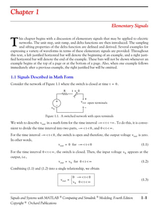
![Chapter 1 Elementary Signals
Thus, the square waveform of Figure 1.10 can be expressed as the summation of (1.8) through
(1.11), that is,
v ( t ) = v1 ( t ) + v2 ( t ) + v3 ( t ) + v4 ( t )
= A [ u 0 ( t ) – u 0 ( t – T ) ] – A [ u 0 ( t – T ) – u 0 ( t – 2T ) ] (1.12)
+A [ u 0 ( t – 2T ) – u 0 ( t – 3T ) ] – A [ u 0 ( t – 3T ) – u 0 ( t – 4T ) ]
Combining like terms, we obtain
v ( t ) = A [ u 0 ( t ) – 2u 0 ( t – T ) + 2u 0 ( t – 2T ) – 2u 0 ( t – 3T ) + … ] (1.13)
Example 1.3
Express the symmetric rectangular pulse of Figure 1.11 as a sum of unit step functions.
i(t)
A
t
–T ⁄ 2 0 T⁄2
Figure 1.11. Symmetric rectangular pulse for Example 1.3
Solution:
This pulse has height A , starts at t = – T ⁄ 2 , and terminates at t = T ⁄ 2 . Therefore, with refer-
ence to Figures 1.5 and 1.8 (b), we obtain
i ( t ) = Au 0 t + -- – Au 0 t – -- = A u 0 t + -- – u 0 t – --
T T T T
-
2
-
-
2
- (1.14)
2 2
Example 1.4
Express the symmetric triangular waveform of Figure 1.12 as a sum of unit step functions.
v(t)
1
t
–T ⁄ 2 0 T⁄2
Figure 1.12. Symmetric triangular waveform for Example 1.4
Solution:
1−6 Signals and Systems with MATLAB Computing and Simulink Modeling, Fourth Edition
Copyright © Orchard Publications](https://image.slidesharecdn.com/signalsandsystemswithmatlabcomputingandsimulinkmodeling-121109110233-phpapp02/85/Signals-and-systems-with-matlab-computing-and-simulink-modeling-21-320.jpg)

![Chapter 1 Elementary Signals
As in the previous example, we first find the equations of the linear segments linear segments
and shown in Figure 1.15.
v(t)
3
2
2t + 1
1 –t+3
t
0 1 2 3
Figure 1.15. Equations for the linear segments of Figure 1.14
Following the same procedure as in the previous examples, we obtain
v ( t ) = ( 2t + 1 ) [ u 0 ( t ) – u 0 ( t – 1 ) ] + 3 [ u 0 ( t – 1 ) – u 0 ( t – 2 ) ]
+ ( – t + 3 ) [ u0 ( t – 2 ) – u0 ( t – 3 ) ]
Multiplying the values in parentheses by the values in the brackets, we obtain
v ( t ) = ( 2t + 1 )u 0 ( t ) – ( 2t + 1 )u 0 ( t – 1 ) + 3u 0 ( t – 1 )
– 3u 0 ( t – 2 ) + ( – t + 3 )u 0 ( t – 2 ) – ( – t + 3 )u 0 ( t – 3 )
v ( t ) = ( 2t + 1 )u 0 ( t ) + [ – ( 2t + 1 ) + 3 ]u 0 ( t – 1 )
+ [ – 3 + ( – t + 3 ) ]u 0 ( t – 2 ) – ( – t + 3 )u 0 ( t – 3 )
and combining terms inside the brackets, we obtain
v ( t ) = ( 2t + 1 )u 0 ( t ) – 2 ( t – 1 )u 0 ( t – 1 ) – t u 0 ( t – 2 ) + ( t – 3 )u 0 ( t – 3 ) (1.18)
Two other functions of interest are the unit ramp function, and the unit impulse or delta function.
We will introduce them with the examples that follow.
Example 1.6
In the network of Figure 1.16 i S is a constant current source and the switch is closed at time
t = 0 . Express the capacitor voltage v C ( t ) as a function of the unit step.
1−8 Signals and Systems with MATLAB Computing and Simulink Modeling, Fourth Edition
Copyright © Orchard Publications](https://image.slidesharecdn.com/signalsandsystemswithmatlabcomputingandsimulinkmodeling-121109110233-phpapp02/85/Signals-and-systems-with-matlab-computing-and-simulink-modeling-23-320.jpg)


![Chapter 1 Elementary Signals
To better understand the delta function δ ( t ) , let us represent the unit step u 0 ( t ) as shown in Fig-
ure 1.20 (a).
1
Figure (a)
0
−ε ε
t
1
Area =1 2ε Figure (b)
0
−ε ε t
Figure 1.20. Representation of the unit step as a limit
The function of Figure 1.20 (a) becomes the unit step as ε → 0 . Figure 1.20 (b) is the derivative of
Figure 1.20 (a), where we see that as ε → 0 , 1 ⁄ 2 ε becomes unbounded, but the area of the rect-
angle remains 1 . Therefore, in the limit, we can think of δ ( t ) as approaching a very large spike or
impulse at the origin, with unbounded amplitude, zero width, and area equal to 1 .
Two useful properties of the delta function are the sampling property and the sifting property.
1.4.1 The Sampling Property of the Delta Function δ ( t )
The sampling property of the delta function states that
f ( t )δ ( t – a ) = f ( a )δ ( t ) (1.35)
or, when a = 0 ,
f ( t )δ ( t ) = f ( 0 )δ ( t ) (1.36)
that is, multiplication of any function f ( t ) by the delta function δ ( t ) results in sampling the func-
tion at the time instants where the delta function is not zero. The study of discrete−time systems is
based on this property.
Proof:
Since δ ( t ) = 0 for t < 0 and t > 0 then,
f ( t )δ ( t ) = 0 for t < 0 and t > 0 (1.37)
We rewrite f ( t ) as
f(t) = f(0) + [f(t) – f(0)] (1.38)
Integrating (1.37) over the interval – ∞ to t and using (1.38), we obtain
1−12 Signals and Systems with MATLAB Computing and Simulink Modeling, Fourth Edition
Copyright © Orchard Publications](https://image.slidesharecdn.com/signalsandsystemswithmatlabcomputingandsimulinkmodeling-121109110233-phpapp02/85/Signals-and-systems-with-matlab-computing-and-simulink-modeling-27-320.jpg)
![The Delta Function
t t t
∫– ∞ f ( τ )δ ( τ ) dτ = ∫– ∞ f ( 0 )δ ( τ ) dτ + ∫–∞ [ f ( τ ) – f ( 0 ) ]δ ( τ ) dτ (1.39)
The first integral on the right side of (1.39) contains the constant term f ( 0 ) ; this can be written
outside the integral, that is,
t t
∫– ∞ f ( 0 )δ ( τ ) dτ = f ( 0 ) ∫– ∞ δ ( τ ) d τ (1.40)
The second integral of the right side of (1.39) is always zero because
δ ( t ) = 0 for t < 0 and t > 0
and
[f(τ ) – f(0 ) ] τ=0
= f(0 ) – f( 0) = 0
Therefore, (1.39) reduces to
t t
∫– ∞ f ( τ )δ ( τ ) dτ = f ( 0 ) ∫– ∞ δ ( τ ) d τ (1.41)
Differentiating both sides of (1.41), and replacing τ with t , we obtain
f ( t )δ ( t ) = f ( 0 )δ ( t )
(1.42)
Sampling Property of δ ( t )
1.4.2 The Sifting Property of the Delta Function δ ( t )
The sifting property of the delta function states that
∞
∫–∞ f ( t )δ ( t – α ) dt = f(α) (1.43)
that is, if we multiply any function f ( t ) by δ ( t – α ) , and integrate from – ∞ to +∞ , we will obtain
the value of f ( t ) evaluated at t = α .
Proof:
Let us consider the integral
b
∫a f ( t )δ ( t – α ) dt where a < α < b (1.44)
We will use integration by parts to evaluate this integral. We recall from the derivative of prod-
ucts that
d ( xy ) = xdy + ydx or xdy = d ( xy ) – ydx (1.45)
and integrating both sides we obtain
Signals and Systems with MATLAB Computing and Simulink Modeling, Fourth Edition 1−13
Copyright © Orchard Publications](https://image.slidesharecdn.com/signalsandsystemswithmatlabcomputingandsimulinkmodeling-121109110233-phpapp02/85/Signals-and-systems-with-matlab-computing-and-simulink-modeling-28-320.jpg)
![Chapter 1 Elementary Signals
∫ x dy = xy – y dx ∫ (1.46)
Now, we let x = f ( t ) ; then, dx = f ′( t ) . We also let dy = δ ( t – α ) ; then, y = u 0 ( t – α ) . By sub-
stitution into (1.44), we obtain
b b
∫a ∫a u0 ( t – α )f ′( t ) dt
b
f ( t )δ ( t – α ) dt = f ( t )u 0 ( t – α ) – (1.47)
a
We have assumed that a < α < b ; therefore, u 0 ( t – α ) = 0 for α < a , and thus the first term of the
right side of (1.47) reduces to f ( b ) . Also, the integral on the right side is zero for α < a , and there-
fore, we can replace the lower limit of integration a by α . We can now rewrite (1.47) as
b b
∫a f ( t )δ ( t – α ) dt = f ( b ) – ∫α f ′ ( t ) d t = f( b) – f( b) + f(α )
and letting a → – ∞ and b → ∞ for any α < ∞ , we obtain
∞
∫–∞ f ( t )δ ( t – α ) dt = f ( α ) (1.48)
Sifting Property of δ ( t )
1.5 Higher Order Delta Functions
An nth-order delta function is defined as the nth derivative of u 0 ( t ) , that is,
n
n δ
δ ( t ) = ---- [ u 0 ( t ) ]
- (1.49)
dt
The function δ' ( t ) is called doublet, δ'' ( t ) is called triplet, and so on. By a procedure similar to the
derivation of the sampling property of the delta function, we can show that
f ( t )δ' ( t – a ) = f ( a )δ' ( t – a ) – f ' ( a )δ ( t – a ) (1.50)
Also, the derivation of the sifting property of the delta function can be extended to show that
∞ n
nd
∫
n
f ( t )δ ( t – α ) dt = ( – 1 ) ------- [ f ( t ) ]
-
n
(1.51)
–∞ dt t=α
1−14 Signals and Systems with MATLAB Computing and Simulink Modeling, Fourth Edition
Copyright © Orchard Publications](https://image.slidesharecdn.com/signalsandsystemswithmatlabcomputingandsimulinkmodeling-121109110233-phpapp02/85/Signals-and-systems-with-matlab-computing-and-simulink-modeling-29-320.jpg)

![Chapter 1 Elementary Signals
v(t) (V)
3
2
1
−1 1 2 3 4 5 6 7
0
t (s)
−1
−2
Figure 1.21. Waveform for Example 1.9
Solution:
a. We begin with the derivation of the equations for the linear segments of the given waveform as
shown in Figure 1.22.
v(t) (V) v(t)
–t+5
3
2 –t+6
1
−1 1 2 3 4 5 6 7
0
t (s)
−1
2t
−2
Figure 1.22. Equations for the linear segments of Figure 1.21
Next, we express v ( t ) in terms of the unit step function u 0 ( t ) , and we obtain
v ( t ) = 2t [ u 0 ( t + 1 ) – u 0 ( t – 1 ) ] + 2 [ u 0 ( t – 1 ) – u 0 ( t – 2 ) ]
+ ( – t + 5 ) [ u0 ( t – 2 ) – u0 ( t – 4 ) ] + [ u0 ( t – 4 ) – u0 ( t – 5 ) ] (1.52)
+ ( – t + 6 ) [ u0 ( t – 5 ) – u0 ( t – 7 ) ]
Multiplying and collecting like terms in (1.52), we obtain
1−16 Signals and Systems with MATLAB Computing and Simulink Modeling, Fourth Edition
Copyright © Orchard Publications](https://image.slidesharecdn.com/signalsandsystemswithmatlabcomputingandsimulinkmodeling-121109110233-phpapp02/85/Signals-and-systems-with-matlab-computing-and-simulink-modeling-31-320.jpg)


![Solutions to End−of−Chapter Exercises
1. We apply the sampling property of the δ ( t ) function for all expressions except (e) where we
apply the sifting property. For part (f) we apply the sampling property of the doublet.
We recall that the sampling property states that f ( t )δ ( t – a ) = f ( a )δ ( t – a ) . Thus,
π π π π
a. sin tδ t – π = sin t
--
- δ t – -- = sin -- δ t – -- = 0.5δ t – --
- - -
6
-
6 t = π⁄6 6 6 6
π
b. cos 2tδ t – π = cos 2t
--
-
δ t – π = cos -- δ t – π = 0
4
--
- - --
-
4 t = π⁄4 2 4
π π
c. cos t δ t – π = -- ( 1 + cos 2t ) π
δ t – -- = -- ( 1 + cos π )δ t – -- = -- ( 1 – 1 )δ t – -- = 0
2 1 1 1
--
- - - - - - -
2 2 2 2 2 2 2
t =π⁄2
π π π
d. tan 2tδ t – π = tan 2t
--
-
π
δ t – -- = tan -- δ t – -- = δ t – --
- - -
8
-
8 t = π⁄8 8 4 8
∞
We recall that the sampling property states that ∫–∞ f ( t )δ ( t – α ) dt = f ( α ) . Thus,
∞
2 –t 2 –t –2
e. ∫– ∞ t e δ ( t – 2 ) dt = t e t=2
= 4e = 0.54
We recall that the sampling property for the doublet states that
f ( t )δ' ( t – a ) = f ( a )δ' ( t – a ) – f ' ( a )δ ( t – a )
Thus,
π π π
sin t δ t – -- = sin t δ t – -- – ---- sin t δ t – --
2 1 2 1 d 2
- - - -
2 t = π⁄2 2 dt t = π⁄2 2
π π
δ t – -- – sin 2t δ t – --
1
f. = -- ( 1 – cos 2t )
1
- - -
2 t = π⁄2 2 t = π⁄2 2
π π π
= -- ( 1 + 1 )δ t – -- – sin πδ t – -- = δ t – --
1 1 1
- - - -
2 2 2 2
2.
– 2t
v( t) = e [ u 0 ( t ) – u 0 ( t – 2 ) ] + ( 10t – 30 ) [ u 0 ( t – 2 ) – u 0 ( t – 3 ) ]
a.
+ ( – 10 t + 50 ) [ u 0 ( t – 3 ) – u 0 ( t – 5 ) ] + ( 10t – 70 ) [ u 0 ( t – 5 ) – u 0 ( t – 7 ) ]
– 2t – 2t
v(t) = e u0 ( t ) – e u 0 ( t – 2 ) + 10tu 0 ( t – 2 ) – 30u 0 ( t – 2 ) – 10tu 0 ( t – 3 ) + 30u 0 ( t – 3 )
– 10tu 0 ( t – 3 ) + 50u 0 ( t – 3 ) + 10tu 0 ( t – 5 ) – 50u 0 ( t – 5 ) + 10tu 0 ( t – 5 )
– 70u 0 ( t – 5 ) – 10tu 0 ( t – 7 ) + 70u 0 ( t – 7 )
Signals and Systems with MATLAB Computing and Simulink Modeling, Fourth Edition 1−25
Copyright © Orchard Publications](https://image.slidesharecdn.com/signalsandsystemswithmatlabcomputingandsimulinkmodeling-121109110233-phpapp02/85/Signals-and-systems-with-matlab-computing-and-simulink-modeling-40-320.jpg)
![Chapter 1 Elementary Signals
– 2t – 2t
v(t) = e u0 ( t ) + ( –e + 10t – 30 )u 0 ( t – 2 ) + ( – 20t + 80 )u 0 ( t – 3 ) + ( 20t – 120 )u 0 ( t – 5 )
+ ( – 10t + 70 )u 0 ( t – 7 )
b.
dv – 2t – 2t – 2t – 2t
----- = – 2e u 0 ( t ) + e δ ( t ) + ( 2e + 10 )u 0 ( t – 2 ) + ( – e + 10t – 30 )δ ( t – 2 )
-
dt
– 20u 0 ( t – 3 ) + ( – 20t + 80 )δ ( t – 3 ) + 20u 0 ( t – 5 ) + ( 20t – 120 )δ ( t – 5 ) (1)
– 10u 0 ( t – 7 ) + ( – 10t + 70 )δ ( t – 7 )
Referring to the given waveform we observe that discontinuities occur only at t = 2 , t = 3 ,
and t = 5 . Therefore, δ ( t ) = 0 and δ ( t – 7 ) = 0 . Also, by the sampling property of the delta
function
– 2t – 2t
( –e + 10t – 30 )δ ( t – 2 ) = ( – e + 10t – 30 ) t=2
δ ( t – 2 ) ≈ – 10δ ( t – 2 )
( – 20t + 80 )δ ( t – 3 ) = ( – 20t + 80 ) t=3
δ ( t – 3 ) = 20δ ( t – 3 )
( 20t – 120 )δ ( t – 5 ) = ( 20t – 120 ) t=5
δ ( t – 5 ) = – 20 δ ( t – 5 )
and with these simplifications (1) above reduces to
– 2t – 2t
dv ⁄ dt = – 2e u 0 ( t ) + 2e u 0 ( t – 2 ) + 10u 0 ( t – 2 ) – 10δ ( t – 2 )
– 20u 0 ( t – 3 ) + 20δ ( t – 3 ) + 20u 0 ( t – 5 ) – 20δ ( t – 5 ) – 10u 0 ( t – 7 )
– 2t
= – 2e [ u 0 ( t ) – u 0 ( t – 2 ) ] – 10δ ( t – 2 ) + 10 [ u 0 ( t – 2 ) – u 0 ( t – 3 ) ] + 20δ ( t – 3 )
– 10 [ u 0 ( t – 3 ) – u 0 ( t – 5 ) ] – 20δ ( t – 5 ) + 10 [ u 0 ( t – 5 ) – u 0 ( t – 7 ) ]
The waveform for dv ⁄ dt is shown below.
dv ⁄ dt (V ⁄ s)
20 δ ( t – 3 )
20
10
1 2 3 4 5 6 7 t (s)
– 10
– 10δ ( t – 2 )
– 20
– 2t – 20 δ ( t – 5 )
– 2e
1−26 Signals and Systems with MATLAB Computing and Simulink Modeling, Fourth Edition
Copyright © Orchard Publications](https://image.slidesharecdn.com/signalsandsystemswithmatlabcomputingandsimulinkmodeling-121109110233-phpapp02/85/Signals-and-systems-with-matlab-computing-and-simulink-modeling-41-320.jpg)


![Properties and Theorems of the Laplace Transform
2.2.1 Linearity Property
The linearity property states that if
f 1 ( t ), f 2 ( t ), …, f n ( t )
have Laplace transforms
F 1 ( s ), F 2 ( s ), …, F n ( s )
respectively, and
c 1 , c 2 , …, c n
are arbitrary constants, then,
c1 f1 ( t ) + c2 f2 ( t ) + … + cn fn ( t ) ⇔ c 1 F1 ( s ) + c2 F2 ( s ) + … + cn Fn ( s ) (2.11)
Proof:
∞
L { c1 f1 ( t ) + c2 f2 ( t ) + … + cn fn ( t ) } = ∫t 0
[ c 1 f 1 ( t ) + c 2 f 2 ( t ) + … + c n f n ( t ) ] dt
∞ ∞ ∞
– st – st – st
= c1 ∫t 0
f1 ( t ) e dt + c 2 ∫t 0
f2 ( t ) e dt + … + c n ∫t 0
fn ( t ) e dt
= c1 F1 ( s ) + c2 F2 ( s ) + … + cn Fn ( s )
Note 1:
It is desirable to multiply f ( t ) by the unit step function u 0 ( t ) to eliminate any unwanted non−
zero values of f ( t ) for t < 0 .
2.2.2 Time Shifting Property
The time shifting property states that a right shift in the time domain by a units, corresponds to
– as
multiplication by e in the complex frequency domain. Thus,
– as
f ( t – a )u 0 ( t – a ) ⇔ e F(s) (2.12)
Proof:
a ∞
– st – st
L { f ( t – a )u 0 ( t – a ) } = ∫0 0e dt + ∫ a f( t – a )e dt (2.13)
Now, we let t – a = τ ; then, t = τ + a and dt = dτ . With these substitutions and with a → 0 ,
the second integral on the right side of (2.13) is expressed as
∞ ∞
–s ( τ + a ) – as – sτ – as
∫0 f(τ)e dτ = e ∫0 f ( τ ) e dτ = e F(s)
Signals and Systems with MATLAB Computing and Simulink Modeling, Fourth Edition 2−3
Copyright © Orchard Publications](https://image.slidesharecdn.com/signalsandsystemswithmatlabcomputingandsimulinkmodeling-121109110233-phpapp02/85/Signals-and-systems-with-matlab-computing-and-simulink-modeling-44-320.jpg)

![Properties and Theorems of the Laplace Transform
d- −
f ' ( t ) = ---- f ( t ) ⇔ sF ( s ) – f ( 0 ) (2.16)
dt
Proof:
∞
– st
L {f '(t)} = ∫0 f ' ( t ) e dt
Using integration by parts where
∫ v du = uv – u dv ∫ (2.17)
– st – st
we let du = f ' ( t ) and v = e . Then, u = f ( t ) , dv = – se , and thus
∞
– st ∞ – st – st a
L { f ' ( t ) } = f ( t )e
0
−
+s ∫0 −
f(t)e dt = lim
a→∞
f ( t )e
0
−
+ sF ( s )
– sa − −
= lim [ e f ( a ) – f ( 0 ) ] + sF ( s ) = 0 – f ( 0 ) + sF ( s )
a→∞
The time differentiation property can be extended to show that
d2
------- f ( t ) ⇔ s 2 F ( s ) – sf ( 0 − ) – f ' ( 0 − )
- (2.18)
2
dt
d3
------- f ( t ) ⇔ s 3 F ( s ) – s 2 f ( 0 − ) – sf ' ( 0 − ) – f '' ( 0 − )
- (2.19)
3
dt
and in general
n
d
------- f ( t ) ⇔ s n F ( s ) – s n – 1 f ( 0 − ) – s n – 2 f ' ( 0 − ) – … – f
- n–1
(0 )
−
(2.20)
n
dt
To prove (2.18), we let
d
g ( t ) = f ' ( t ) = ---- f ( t )
-
dt
and as we found above,
−
L { g ' ( t ) } = sL { g ( t ) } – g ( 0 )
Then,
− − −
L { f '' ( t ) } = sL { f ' ( t ) } – f ' ( 0 ) = s [ sL [ f ( t ) ] – f ( 0 ) ] – f ' ( 0 )
− −
= s 2 F ( s ) – sf ( 0 ) – f ' ( 0 )
Relations (2.19) and (2.20) can be proved by similar procedures.
Signals and Systems with MATLAB Computing and Simulink Modeling, Fourth Edition 2−5
Copyright © Orchard Publications](https://image.slidesharecdn.com/signalsandsystemswithmatlabcomputingandsimulinkmodeling-121109110233-phpapp02/85/Signals-and-systems-with-matlab-computing-and-simulink-modeling-46-320.jpg)
![Chapter 2 The Laplace Transformation
We must remember that the terms f ( 0 − ), f ' ( 0 − ), f '' ( 0 − ) , and so on, represent the initial condi-
tions. Therefore, when all initial conditions are zero, and we differentiate a time function f ( t ) n
times, this corresponds to F ( s ) multiplied by s to the nth power.
2.2.6 Differentiation in Complex Frequency Domain Property
This property states that differentiation in complex frequency domain and multiplication by minus
one, corresponds to multiplication of f ( t ) by t in the time domain. In other words,
d
tf ( t ) ⇔ – ---- F ( s )
- (2.21)
ds
Proof:
∞
– st
L { f( t)} = F( s) = ∫0 f ( t ) e dt
Differentiating with respect to s and applying Leibnitz’s rule* for differentiation under the integral,
we obtain
∞ ∞ ∞ ∞
d d – st ∂ –st – st – st
---- F ( s ) = ----
ds
-
ds
-
∫0 f( t)e dt = ∫0 ∂s
e f ( t )dt = ∫0 –t e f ( t )dt = – ∫0 [ tf ( t ) ] e dt = – L [ tf ( t ) ]
In general,
n
n nd
t f ( t ) ⇔ ( – 1 ) ------- F ( s )
-
n
(2.22)
ds
The proof for n ≥ 2 follows by taking the second and higher−order derivatives of F ( s ) with
respect to s .
2.2.7 Integration in Time Domain Property
This property states that integration in time domain corresponds to F ( s ) divided by s plus the ini-
tial value of f ( t ) at t = 0 − , also divided by s . That is,
b
* This rule states that if a function of a parameter α is defined by the equation F ( α ) = ∫a f ( x, α ) dx where f is some known
function of integration x and the parameter α , a and b are constants independent of x and α , and the partial derivative
dF b
∂( x, α )
∂f ⁄ ∂α exists and it is continuous, then ------ =
dα
- ∫a ----------------- dx .
∂( α )
2−6 Signals and Systems with MATLAB Computing and Simulink Modeling, Fourth Edition
Copyright © Orchard Publications](https://image.slidesharecdn.com/signalsandsystemswithmatlabcomputingandsimulinkmodeling-121109110233-phpapp02/85/Signals-and-systems-with-matlab-computing-and-simulink-modeling-47-320.jpg)


![Chapter 2 The Laplace Transformation
Proof:
From the time domain differentiation property,
d
---- f ( t ) ⇔ sF ( s ) – f ( 0 − )
-
dt
or
d ∞
d
---- f ( t ) e –st dt
∫0
−
L ---- f ( t ) = sF ( s ) – f ( 0 ) =
- -
dt dt
Taking the limit of both sides by letting s → ∞ , we obtain
T
d – st
∫ ----- f ( t ) e
−
lim [ sF ( s ) – f ( 0 ) ] = lim lim dt
s→∞ s→∞ T → ∞ ε dt
ε→0
Interchanging the limiting process, we obtain
T
d – st
T → ∞ ∫ ε dt
−
lim [ sF ( s ) – f ( 0 ) ] = lim ---- f ( t )
- lim e dt
s→∞ s→∞
ε→0
and since
– st
lim e = 0
s→∞
the above expression reduces to
−
lim [ sF ( s ) – f ( 0 ) ] = 0
s→∞
or
−
lim sF ( s ) = f ( 0 )
s→∞
2.2.11 Final Value Theorem
The final value theorem states that the final value f ( ∞ ) of the time function f ( t ) can be found
from its Laplace transform multiplied by s , then, letting s → 0 . That is,
lim f ( t ) = lim sF ( s ) = f ( ∞ ) (2.33)
t→∞ s→0
Proof:
From the time domain differentiation property,
d
---- f ( t ) ⇔ sF ( s ) – f ( 0 − )
-
dt
or
2−10 Signals and Systems with MATLAB Computing and Simulink Modeling, Fourth Edition
Copyright © Orchard Publications](https://image.slidesharecdn.com/signalsandsystemswithmatlabcomputingandsimulinkmodeling-121109110233-phpapp02/85/Signals-and-systems-with-matlab-computing-and-simulink-modeling-51-320.jpg)
![Properties and Theorems of the Laplace Transform
d ∞
d
---- f ( t ) e –st dt
∫0
−
L ---- f ( t ) = sF ( s ) – f ( 0 ) =
- -
dt dt
Taking the limit of both sides by letting s → 0 , we obtain
T
d – st
∫ ---- f ( t ) e
−
lim [ sF ( s ) – f ( 0 ) ] = lim lim - dt
s→0 s→0 T → ∞ ε dt
ε→0
and by interchanging the limiting process, the expression above is written as
T
d – st
∫ ----- f ( t )
−
lim [ sF ( s ) – f ( 0 ) ] = lim lim e dt
s→0 T→∞ ε
dt s→0
ε→0
Also, since
– st
lim e = 1
s→0
it reduces to
T T
d
∫ ∫ε f ( t )
− −
lim [ sF ( s ) – f ( 0 ) ] = lim ---- f ( t ) dt = lim
- = lim [ f ( T ) – f ( ε ) ] = f ( ∞ ) – f ( 0 )
s→0 T→∞ ε dt T→∞ T→∞
ε→0 ε→0 ε→0
Therefore,
lim sF ( s ) = f ( ∞ )
s→0
2.2.12 Convolution in Time Domain Property
Convolution* in the time domain corresponds to multiplication in the complex frequency domain,
that is,
f 1 ( t )*f 2 ( t ) ⇔ F 1 ( s )F 2 ( s ) (2.34)
* Convolution is the process of overlapping two time functions f 1 ( t ) and f 2 ( t ) . The convolution integral indicates
the amount of overlap of one function as it is shifted over another function The convolution of two time functions
∞
f1 ( t ) and f2 ( t ) is denoted as f 1 ( t )*f 2 ( t ) , and by definition, f 1 ( t )*f 2 ( t ) = ∫–∞ f1 ( τ )f2 ( t – τ ) dτ where τ is a dummy
variable. Convolution is discussed in detail in Chapter 6.
Signals and Systems with MATLAB Computing and Simulink Modeling, Fourth Edition 2−11
Copyright © Orchard Publications](https://image.slidesharecdn.com/signalsandsystemswithmatlabcomputingandsimulinkmodeling-121109110233-phpapp02/85/Signals-and-systems-with-matlab-computing-and-simulink-modeling-52-320.jpg)


![Chapter 2 The Laplace Transformation
n – at n!
t e u 0 ( t ) ⇔ ------------------------
n+1
- (2.61)
(s + a)
for σ > – a .
2.3.8 The Laplace Transform of sin ωt u 0 ( t )
We apply the definition
∞ a
– st – st
L { sin ωt u 0 ( t ) } = ∫0 ( sin ωt ) e dt = lim
a→∞ 0 ∫ ( sin ωt ) e dt
and from tables of integrals*
ax
∫ e sin bx dx = e ( a sin bx – b cos bx - )
ax
-----------------------------------------------------
2 2
a +b
Then,
– st a
e ( – s sin ωt – ω cos ωt - )
L { sin ωt u 0 ( t ) } = lim ----------------------------------------------------------
a→∞ 2
s +ω
2
0
– as
e ( – s sin ωa – ω cos ωa ) ω ω
= lim ------------------------------------------------------------- + ---------------- = ----------------
- - -
a→∞ 2
s +ω
2 2
s +ω
2 2
s +ω
2
Thus, we have obtained the transform pair
ω
sin ωt u 0 t ⇔ ----------------
2
-
2
(2.62)
s +ω
for σ > 0 .
2.3.9 The Laplace Transform of cos ω t u 0 ( t )
We apply the definition
∞ a
– st – st
L { cos ω t u 0 ( t ) } = ∫0 ( cos ωt ) e dt = lim
a→∞ 0 ∫ ( cos ωt ) e dt
1- jωt – jωt – at 1-
* This can also be derived from sin ωt = ---- ( e – e ) , and the use of (2.55) where e u 0 ( t ) ⇔ ---------- . By the linearity
j2 s+a
property, the sum of these terms corresponds to the sum of their Laplace transforms. Therefore,
1-
L [ sin ωtu 0 ( t ) ] = ---- 1 - 1 ω
------------- – -------------- = -----------------
j2 s – jω s + jω
s2 + ω2
2−20 Signals and Systems with MATLAB Computing and Simulink Modeling, Fourth Edition
Copyright © Orchard Publications](https://image.slidesharecdn.com/signalsandsystemswithmatlabcomputingandsimulinkmodeling-121109110233-phpapp02/85/Signals-and-systems-with-matlab-computing-and-simulink-modeling-61-320.jpg)
![The Laplace Transform of Common Functions of Time
and from tables of integrals*
ax
e ( acos bx + b sin bx )
∫
ax
e cos bx dx = -----------------------------------------------------
-
2 2
a +b
Then,
– st a
e ( – s cos ωt + ω sin ωt )
L { cos ω t u 0 ( t ) } = lim ----------------------------------------------------------
-
a→∞ 2
s +ω
2
0
– as
= lim e ( – s cos ωa + ω sin ωa ) + ---------------- = ----------------
-------------------------------------------------------------
- s - s -
a→∞ 2
s +ω
2 2
s +ω
2 2
s +ω
2
Thus, we have the fransform pair
s
cos ω t u 0 t ⇔ ----------------
2
-
2
(2.63)
s +ω
for σ > 0 .
– at
2.3.10 The Laplace Transform of e sin ωt u 0 ( t )
From (2.62),
ω
sin ωtu 0 t ⇔ ----------------
2
-
2
s +ω
Using the frequency shifting property of (2.14), that is,
– at
e f(t) ⇔ F(s + a ) (2.64)
we replace s with s + a , and we obtain
– at ω
e sin ωt u 0 ( t ) ⇔ ------------------------------
2
-
2
(2.65)
(s + a) + ω
for σ > 0 and a > 0 .
1 jωt – jωt
* We can use the relation cos ωt = -- ( e + e
- ) and the linearity property, as in the derivation of the transform of
2
d- −
sin ω t on the footnote of the previous page. We can also use the transform pair ---- f ( t ) ⇔ sF ( s ) – f ( 0 ) ; this is the time
dt
differentiation property of (2.16). Applying this transform pair for this derivation, we obtain
1 d- 1 d- 1 ω s
L [ cos ω tu 0 ( t ) ] = L --- ---- sin ω tu 0 ( t ) = --- L ---- sin ω tu 0 ( t ) = --- s ----------------- = -----------------
- - -
ω dt ω dt ω s2 + ω2 s + ω2
2
Signals and Systems with MATLAB Computing and Simulink Modeling, Fourth Edition 2−21
Copyright © Orchard Publications](https://image.slidesharecdn.com/signalsandsystemswithmatlabcomputingandsimulinkmodeling-121109110233-phpapp02/85/Signals-and-systems-with-matlab-computing-and-simulink-modeling-62-320.jpg)

![The Laplace Transform of Common Waveforms
2.4 The Laplace Transform of Common Waveforms
In this section, we will present procedures for deriving the Laplace transform of common wave-
forms using the transform pairs of Tables 1 and 2. The derivations are described in Subsections
2.4.1 through 2.4.5 below.
2.4.1 The Laplace Transform of a Pulse
The waveform of a pulse, denoted as f P ( t ) , is shown in Figure 2.1.
fP ( t )
A
0 a t
Figure 2.1. Waveform for a pulse
We first express the given waveform as a sum of unit step functions as we’ve learned in Chapter
1. Then,
fP ( t ) = A [ u0 ( t ) – u0 ( t – a ) ] (2.67)
From Table 2.1, Page 2−13,
– as
f ( t – a )u 0 ( t – a ) ⇔ e F(s)
and from Table 2.2, Page 2−22
u0 ( t ) ⇔ 1 ⁄ s
Thus,
Au 0 ( t ) ⇔ A ⁄ s
and
– as A
Au 0 ( t – a ) ⇔ e ---
-
s
Then, in accordance with the linearity property, the Laplace transform of the pulse of Figure 2.1
is
A –as A A – as
A [ u 0 ( t ) – u 0 ( t – a ) ] ⇔ --- – e --- = --- ( 1 – e )
- - -
s s s
2.4.2 The Laplace Transform of a Linear Segment
The waveform of a linear segment, denoted as f L ( t ) , is shown in Figure 2.2.
Signals and Systems with MATLAB Computing and Simulink Modeling, Fourth Edition 2−23
Copyright © Orchard Publications](https://image.slidesharecdn.com/signalsandsystemswithmatlabcomputingandsimulinkmodeling-121109110233-phpapp02/85/Signals-and-systems-with-matlab-computing-and-simulink-modeling-64-320.jpg)

![The Laplace Transform of Common Waveforms
fT ( t )
1 t –t+2
1 2 t
0
Figure 2.5. Triangular waveform with the equations of the linear segments
Next, we express the given waveform in terms of the unit step function.
fT ( t ) = t [ u0 ( t ) – u0 ( t – 1 ) ] + ( – t + 2 ) [ u0 ( t – 1 ) – u0 ( t – 2 ) ]
= tu 0 ( t ) – tu 0 ( t – 1 ) – tu 0 ( t – 1 ) + 2u 0 ( t – 1 ) + tu 0 ( t – 2 ) – 2u 0 ( t – 2 )
Collecting like terms, we obtain
f T ( t ) = tu 0 ( t ) – 2 ( t – 1 )u 0 ( t – 1 ) + ( t – 2 )u 0 ( t – 2 )
From Table 2.1, Page 2−13,
– as
f ( t – a )u 0 ( t – a ) ⇔ e F(s)
and from Table 2.2, Page 2−22,
1-
tu 0 ( t ) ⇔ ---
2
s
Then,
1- –s 1 – 2s 1
tu 0 ( t ) – 2 ( t – 1 )u 0 ( t – 1 ) + ( t – 2 )u 0 ( t – 2 ) ⇔ --- – 2e --- + e ---
-
2
-
2
2
s s s
or
1- –s – 2s
tu 0 ( t ) – 2 ( t – 1 )u 0 ( t – 1 ) + ( t – 2 )u 0 ( t – 2 ) ⇔ --- ( 1 – 2e + e )
2
s
Therefore, the Laplace transform of the triangular waveform of Figure 2.4 is
1- –s 2
f T ( t ) ⇔ --- ( 1 – e )
2
(2.69)
s
2.4.4 The Laplace Transform of a Rectangular Periodic Waveform
The waveform of a rectangular periodic waveform, denoted as f R ( t ) , is shown in Figure 2.6. This
is a periodic waveform with period T = 2a , and we can apply the time periodicity property
T
– sτ
∫0 f ( τ ) e dτ
L { f ( τ ) } = -------------------------------
-
– sT
1–e
Signals and Systems with MATLAB Computing and Simulink Modeling, Fourth Edition 2−25
Copyright © Orchard Publications](https://image.slidesharecdn.com/signalsandsystemswithmatlabcomputingandsimulinkmodeling-121109110233-phpapp02/85/Signals-and-systems-with-matlab-computing-and-simulink-modeling-66-320.jpg)

![Using MATLAB for Finding the Laplace Transforms of Time Functions
where the denominator represents the periodicity of f ( t ) .
f HW ( t )
π 2π 3π 4π 5π
Figure 2.7. Half-rectified sine waveform*
For this waveform,
2π π
1 – st 1 – st
L { f HW ( t ) } = --------------------
1–e
– 2πs
-
∫0 f( t)e dt = --------------------
1–e
– 2πs
-
∫0 sin t e dt
π
– st – πs
1 - e ( s sin t – cos t - ) 1 ( 1 + e )-
= -------------------- -----------------------------------------
– 2πs 2
= ------------------ -------------------------
2 – 2πs
1–e s +1 (s + 1) (1 – e )
0
– πs
1 (1 + e )
L { f HW ( t ) } = ------------------ -----------------------------------------------
2 – πs – πs
(s + 1) (1 + e )(1 – e )
1
f HW ( t ) ⇔ ------------------------------------------
2 – πs
(2.71)
(s + 1)(1 – e )
2.5 Using MATLAB for Finding the Laplace Transforms of Time Functions
We can use the MATLAB function laplace to find the Laplace transform of a time function. For
examples, please type
help laplace
in MATLAB’s Command prompt.
We will be using this function extensively in the subsequent chapters of this book.
* This waveform was produced with the following MATLAB script:
t=0:pi/64:5*pi; x=sin(t); y=sin(t−2*pi); z=sin(t−4*pi); plot(t,x,t,y,t,z); axis([0 5*pi 0 1])
Signals and Systems with MATLAB Computing and Simulink Modeling, Fourth Edition 2−27
Copyright © Orchard Publications](https://image.slidesharecdn.com/signalsandsystemswithmatlabcomputingandsimulinkmodeling-121109110233-phpapp02/85/Signals-and-systems-with-matlab-computing-and-simulink-modeling-68-320.jpg)


![Chapter 2 The Laplace Transformation
b.
d –s +9
2 2 2 2
d s + 3 – s ( 2s )
2 ( – 1 ) ------- --------------- = 2 ---- ---------------------------------- = 2 ---- --------------------
2 d s
- - - - - -
2 2 2 ds 2
(s + 9)
ds 2 2
ds s + 3 2
(s + 9)
2 2 2 2
( s + 9 ) ( – 2s ) – 2 ( s + 9 ) ( 2s ) ( – s + 9 - )
= 2 ⋅ -------------------------------------------------------------------------------------------------
4
2
(s + 9)
2 2 3 3
( s + 9 ) ( – 2s ) – 4s ( – s + 9 - ) – 2s – 18s + 4s – 36s
= 2 ⋅ ------------------------------------------------------------------- = 2 ⋅ -------------------------------------------------------
3 3
-
2 2
(s + 9) (s + 9)
3 2
2s – 54s 2s ( s – 27 ) 4s ( s 2 – 27 )
= 2 ⋅ ---------------------- = 2 ⋅ -------------------------- = --------------------------
3 3
- -
2 2 3
(s + 9) (s + 9) 2
(s + 9)
c.
2×5 10
------------------------------ = ------------------------------
-
2 2 2
(s + 5) + 5 ( s + 5 ) + 25
d.
8(s + 3) 8(s + 3)
----------------------------- = ------------------------------
- -
2 2 2
(s + 3) + 4 ( s + 3 ) + 16
e.
– ( π ⁄ 4 )s
cos t π⁄4
δ ( t – π ⁄ 4 ) = ( 2 ⁄ 2 )δ ( t – π ⁄ 4 ) and ( 2 ⁄ 2 )δ ( t – π ⁄ 4 ) ⇔ ( 2 ⁄ 2 )e
5.
a.
– 3s
--- + 15 = -- e 1 + 3
5- ----- 5 –3s
5tu 0 ( t – 3 ) = [ 5 ( t – 3 ) + 15 ]u 0 ( t – 3 ) ⇔ e - - --
-
2 s s s
s
b.
2 2
( 2t – 5t + 4 )u 0 ( t – 3 ) = [ 2 ( t – 3 ) + 12t – 18 – 5t + 4 ]u 0 ( t – 3 )
2
= [ 2 ( t – 3 ) + 7t – 14 ]u 0 ( t – 3 )
2
= [ 2 ( t – 3 ) + 7 ( t – 3 ) + 21 – 14 ]u 0 ( t – 3 )
– 3s 2 × 2! 7 7
------------- + --- + --
2
= [ 2 ( t – 3 ) + 7 ( t – 3 ) + 7 ]u 0 ( t – 3 ) ⇔ e - - -
3 2 s
s s
c.
– 2t –2 ( t – 2 ) –4
( t – 3 )e u 0 ( t – 2 ) = [ ( t – 2 ) – 1 ]e ⋅ e u0 ( t – 2 )
–4 – 2s 1 1 –4 – 2s – ( s + 1 )
⇔e ⋅e ------------------ – --------------- = e ⋅ e
- ------------------
-
2 (s + 2) 2
(s + 2) (s + 2)
2−34 Signals and Systems with MATLAB Computing and Simulink Modeling, Fourth Edition
Copyright © Orchard Publications](https://image.slidesharecdn.com/signalsandsystemswithmatlabcomputingandsimulinkmodeling-121109110233-phpapp02/85/Signals-and-systems-with-matlab-computing-and-simulink-modeling-75-320.jpg)
![Solutions to End−of−Chapter Exercises
d.
2(t – 2) –2 ( t – 3 ) –2
( 2t – 4 )e u 0 ( t – 3 ) = [ 2 ( t – 3 ) + 6 – 4 ]e ⋅ e u0 ( t – 3 )
–2 – 3s 2 2 –2 – 3s s+4
⇔e ⋅e ------------------ + --------------- = 2e ⋅ e
- ------------------
(s + 3)
2 (s + 3) (s + 3)
2
e.
– 3t 1 d s+3 - d- s+3
4te ( cos 2t )u 0 ( t ) ⇔ 4 ( – 1 ) ---- ----------------------------- = – 4 ---- ----------------------------------
- -
ds ( s + 3 ) 2 + 2 2 ds s 2 + 6s + 9 + 4
2
d s+3 s + 6s + 13 – ( s + 3 ) ( 2s + 6 )
⇔ – 4 ---- ---------------------------- = – 4 -----------------------------------------------------------------------
- - -
ds s 2 + 6s + 13 2 2
( s + 6s + 13 )
2 2 2
s + 6s + 13 – 2s – 6s – 6s – 18 4 ( s + 6s + 5 )
⇔ – 4 ----------------------------------------------------------------------------- = -----------------------------------
2
- -
2 2
( s + 6s + 13 ) 2
( s + 6s + 13 )
6.
a.
---- f ( t ) ⇔ sF ( s ) – f ( 0 − ) −
3 d
sin 3t ⇔ ---------------
2
-
2
- f ( 0 ) = sin 3t t=0
= 0
s +3 dt
d 3 3s
( sin 3t ) ⇔ s --------------- – 0 = -------------
- -
dt 2
s +3
2 2
s +9
b.
---- f ( t ) ⇔ sF ( s ) – f ( 0 − ) −
– 4t 3 d – 4t
3e ⇔ ----------
- - f ( 0 ) = 3e = 3
s+4 dt t=0
d – 4t 3 3s 3 ( s + 4 ) – 12
( 3e ) ⇔ s ---------- – 3 = ---------- – ------------------- = ----------
- - -
dt s+4 s+4 s+4 s+4
c.
2
s 2 2 d s
cos 2t ⇔ ---------------
2
-
2
t cos 2t ⇔ ( – 1 ) ------- -------------
-
2 2
-
s +2 ds s + 4
2 2 2
d s + 4 – s ( 2s ) 2 2 2
---- -------------------------------- = ---- -------------------- = ( s + 4 ) ( – 2s ) – ( – s + 4 ) ( s + 4 )2 ( 2s )
d –s + 4
- - - - ------------------------------------------------------------------------------------------------
-
ds 2 2 ds 2 2 4
(s + 4) (s + 4) 2
(s + 4)
2 2 3 3 2
( s + 4 ) ( – 2s ) – ( – s + 4 ) ( 4s ) – 2s – 8s + 4s – 16s 2s ( s – 12 )
= ----------------------------------------------------------------------- = ---------------------------------------------------- = --------------------------
- - -
2 3 2 3 2 3
(s + 4) (s + 4) (s + 4)
Thus,
2
2 2s ( s – 12 )
t cos 2t ⇔ --------------------------
3
-
2
(s + 4)
and
Signals and Systems with MATLAB Computing and Simulink Modeling, Fourth Edition 2−35
Copyright © Orchard Publications](https://image.slidesharecdn.com/signalsandsystemswithmatlabcomputingandsimulinkmodeling-121109110233-phpapp02/85/Signals-and-systems-with-matlab-computing-and-simulink-modeling-76-320.jpg)
![Chapter 2 The Laplace Transformation
d 2 −
( t cos 2t ) ⇔ sF ( s ) – f ( 0 )
dt
2
2s ( s – 12 ) 2 2
2s ( s – 12 )
⇔ s -------------------------- – 0 = -----------------------------
3
- -
2 3
(s + 4) 2
(s + 4)
d.
2 -
sin 2 t ⇔ --------------- e
– 2t 2
sin 2t ⇔ ---------------------------
- ---- f ( t ) ⇔ sF ( s ) – f ( 0 − )
d-
2 2 2 dt
s +2 (s + 2) + 4
d –2t 2 2s
( e sin 2t ) ⇔ s --------------------------- – 0 = ---------------------------
- -
dt (s + 2) + 4
2
(s + 2) + 4
2
e.
2 – 2t
---- f ( t ) ⇔ sF ( s ) – f ( 0 − )
2 2! 2! d
t ⇔ ----
-
3
t e ⇔ ------------------
3
-
s (s + 2) dt
d 2 –2t 2! 2s
( t e ) ⇔ s ------------------ – 0 = ------------------
dt (s + 2)
3
(s + 2)
3
7.
a.
1 - sin t sin t
sin t ⇔ ------------- but to find L -------- we must first show that the limit lim -------- exists. Since
2
- -
s +1 t t→0 t
∞
sin t 1
∫s
sin x
lim ---------- = 1 , this condition is satisfied and thus -------- ⇔
- ------------- ds . From tables of integrals,
2
-
x→0 x t s +1
1 1 –1 1 - –1
∫ x 2 + a 2 dx
----------------
a
-
2
s +1
∫
= -- tan ( x ⁄ a ) + C . Then, ------------- ds = tan ( 1 ⁄ s ) + C and the constant of integra-
tion C is evaluated from the final value theorem. Thus,
–1 sin - t –1
lim f ( t ) = lim sF ( s ) = lim s [ tan ( 1 ⁄ s ) + C ] = 0 and -------- ⇔ tan ( 1 ⁄ s )
t→∞ s→0 s→0 t
b.
t −
sin t –1 F( s) f (0 )
From (a) above, -------- ⇔ tan ( 1 ⁄ s ) and since
-
t ∫ –∞
f ( τ ) dτ ⇔ ---------- + ------------ , it follows that
s s
-
t
sin τ 1 –1
∫0 ---------- dτ ⇔ -- tan
τ s
- (1 ⁄ s)
c.
From (a) above -------- ⇔ tan ( 1 ⁄ s ) and since f ( at ) ⇔ -- F - , it follows that
sin t –1 1 s
- - -
t a a
2−36 Signals and Systems with MATLAB Computing and Simulink Modeling, Fourth Edition
Copyright © Orchard Publications](https://image.slidesharecdn.com/signalsandsystemswithmatlabcomputingandsimulinkmodeling-121109110233-phpapp02/85/Signals-and-systems-with-matlab-computing-and-simulink-modeling-77-320.jpg)
![Solutions to End−of−Chapter Exercises
–1
----------- ⇔ 1 tan 1 ⁄ s or ----------- ⇔ tan –1( a ⁄ s )
sin at - --
- --------
- sin at -
at a a t
d.
∞
s cos t s
cos t ⇔ ------------- , --------- ⇔
2
s +1
-
t
-
∫s s2 + 1 ds , and from tables of integrals,
-------------
-
x 1 s 1
∫ ---------------- dx = -- ln ( x + a ) + C . Then, ∫ -------------- ds = -- ln ( s + 1 ) + C and the constant of inte-
2 2 2
- -
2 2 2 2 2
x +a s +1
gration C is evaluated from the final value theorem. Thus,
t −
1 F(s) f (0 )
lim f ( t ) = lim sF ( s ) = lim s -- ln ( s + 1 ) + C = 0 and using ∫ f ( τ ) dτ ⇔ ---------- + ------------ we
2
- -
t→∞ s→0 s→0 2 –∞ s s
obtain
∞
cos τ 1
∫t ---------- dτ ⇔ ---- ln ( s 2 + 1 )
τ
-
2s
-
e.
–t ∞
–t 1 - e- 1 1 1
e ⇔ ---------- , ----- ⇔
s+1 t ∫s ----------- ds , and from tables of integrals ∫ --------------- dx
s+1 ax + b
= -- ln ( ax + b ) . Then,
2
-
1
∫ ----------- ds
s+1
= ln ( s + 1 ) + C and the constant of integration C is evaluated from the final value
theorem. Thus,
lim f ( t ) = lim sF ( s ) = lim s [ ln ( s + 1 ) + C ] = 0
t→∞ s→0 s→0
t −
F(s) f (0 )
and using ∫ –∞
f ( τ ) dτ ⇔ ---------- + ------------ , we obtain
s s
-
∞ –τ
e 1
∫t ------ dτ ⇔ -- ln ( s + 1 )
τ
-
s
-
8.
f ST ( t ) A
--- t
-
a
A
a 3a
t
2a
This is a periodic waveform with period T = a , and its Laplace transform is
Signals and Systems with MATLAB Computing and Simulink Modeling, Fourth Edition 2−37
Copyright © Orchard Publications](https://image.slidesharecdn.com/signalsandsystemswithmatlabcomputingandsimulinkmodeling-121109110233-phpapp02/85/Signals-and-systems-with-matlab-computing-and-simulink-modeling-78-320.jpg)
![Chapter 2 The Laplace Transformation
a a
1 - A –st A - – st
F ( s ) = -----------------
1–e
– as ∫ 0
--- te dt = -------------------------
a
-
a(1 – e )
– as ∫0 te dt (1)
and from (2.41), Page 2-14, and limits of integration 0 to a , we obtain
a 0
a – st – st – st – st
– st
∫0 te
a te e te e
L {t} 0
= dt = – --------- – -------
- - = --------- + -------
- -
s 2 s 2
s s
0 a
– as – as
1- ae - e - 1 – as
= --- – ----------- – -------- = --- [ 1 – ( 1 + as )e ]
-
2
2 s 2
s s s
Adding and subtracting as in the last expression above, we obtain
a 1 – as 1 – as
L {t} 0
= --- [ ( 1 + as ) – ( 1 + as )e – as ] = --- [ ( 1 + as ) ( 1 – e ) – as ]
-
2
-
2
s s
By substitution into (1) we obtain
A - 1- – as A – as
F ( s ) = ------------------------- ⋅ --- [ ( 1 + as ) ( 1 – e ) – as ] = ------------------------------ ⋅ [ ( 1 + as ) ( 1 – e ) – as ]
– as 2 2 – as
-
a(1 – e ) s as ( 1 – e )
A ( 1 + as ) Aa A ( 1 + as ) a
= ----------------------- – --------------------------- = ---- ------------------ – ----------------------
- - - - -
2 – as as s – as
as as ( 1 – e ) (1 – e )
9.
This is a periodic waveform with period T = a = π and its Laplace transform is
T π
1 – st 1 - – st
F ( s ) = ------------------
1–e
– sT ∫0 f ( t )e dt = ----------------------
(1 – e )
– πs ∫0 sin te dt
From tables of integrals,
ax
e ( asin bx – b cos bx )
∫
ax
sin bxe dx = -----------------------------------------------------
-
2 2
a +b
Then,
– st π – πs
1 e ( s sin t – cos t ) 1 1+e
F ( s ) = ----------------- ⋅ -----------------------------------------
– πs
-
2
- = ----------------- ⋅ ------------------
– πs
-
2
-
1–e s +1 0
1–e s +1
– πs
1+e πs
= ------------- ⋅ ------------------ = ------------- coth -----
1 1
- - -
2 – πs 2 2
s +1 1–e s +1
The full−rectified waveform can be produced with the MATLAB script
t=0:pi/16:4*pi; x=sin(t); plot(t,abs(x)); axis([0 4*pi 0 1])
2−38 Signals and Systems with MATLAB Computing and Simulink Modeling, Fourth Edition
Copyright © Orchard Publications](https://image.slidesharecdn.com/signalsandsystemswithmatlabcomputingandsimulinkmodeling-121109110233-phpapp02/85/Signals-and-systems-with-matlab-computing-and-simulink-modeling-79-320.jpg)


![Partial Fraction Expansion
3s + 2
F 1 ( s ) = -------------------------
- (3.8)
2
s + 3s + 2
Solution:
Using (3.6), we obtain
3s + 2 3s + 2 r1 r2
F 1 ( s ) = ------------------------- = -------------------------------- = --------------- + ---------------
- - - - (3.9)
2
s + 3s + 2 (s + 1)(s + 2) (s + 1) (s + 2)
The residues are
3s + 2
r 1 = lim ( s + 1 )F ( s ) = ---------------
- = –1 (3.10)
s → –1 (s + 2) s = –1
and
3s + 2
r 2 = lim ( s + 2 )F ( s ) = ---------------
- = 4 (3.11)
s → –2 (s + 1) s = –2
Therefore, we express (3.9) as
3s + 2 - –1 - 4 -
F 1 ( s ) = ------------------------- = --------------- + --------------- (3.12)
2
s + 3s + 2 (s + 1) (s + 2)
and from Table 2.2, Chapter 2, Page 2−22, we find that
– at 1
e u 0 ( t ) ⇔ ----------
- (3.13)
s+a
Therefore,
–1 - 4 - –t – 2t
F 1 ( s ) = --------------- + --------------- ⇔ ( – e + 4e ) u 0 ( t ) = f 1 ( t ) (3.14)
(s + 1) (s + 2)
The residues and poles of a rational function of polynomials such as (3.8), can be found easily
using the MATLAB residue(a,b) function. For this example, we use the script
Ns = [3, 2]; Ds = [1, 3, 2]; [r, p, k] = residue(Ns, Ds)
and MATLAB returns the values
r =
4
-1
p =
-2
-1
k =
[]
Signals and Systems with MATLAB Computing and Simulink Modeling, Fourth Edition 3−3
Copyright © Orchard Publications](https://image.slidesharecdn.com/signalsandsystemswithmatlabcomputingandsimulinkmodeling-121109110233-phpapp02/85/Signals-and-systems-with-matlab-computing-and-simulink-modeling-82-320.jpg)


![Chapter 3 The Inverse Laplace Transformation
Example 3.3
Use the partial fraction expansion method to simplify F 3 ( s ) of (3.23) below, and find the time
domain function f 3 ( t ) corresponding to F 3 ( s ) .
s+3
F 3 ( s ) = ------------------------------------------
- (3.23)
3 2
s + 5s + 12s + 8
Solution:
Let us first express the denominator in factored form to identify the poles of F 3 ( s ) using the
MATLAB factor(s) symbolic function. Then,
syms s; factor(s^3 + 5*s^2 + 12*s + 8)
ans =
(s+1)*(s^2+4*s+8)
The factor(s) function did not factor the quadratic term. We will use the roots(p) function.
p=[1 4 8]; roots_p=roots(p)
roots_p =
-2.0000 + 2.0000i
-2.0000 - 2.0000i
Then,
s+3 s+3
F 3 ( s ) = ------------------------------------------ = ------------------------------------------------------------------------
-
3 2 ( s + 1 ) ( s + 2 + j2 ) ( s + 2 – j2 )
s + 5s + 12s + 8
or
s+3 r1 r2 r 2∗
F 3 ( s ) = ------------------------------------------ = --------------- + --------------------------- + ------------------------
- - - (3.24)
3 2 ( s + 1 ) ( s + 2 + j2 ) ( s + 2 – j 2 )
s + 5s + 12s + 8
The residues are
s+3 -
r 1 = ------------------------- = 2
--
- (3.25)
2 5
s + 4s + 8 s = –1
s+3 1 – j2 1 – j2
r 2 = -----------------------------------------
- = ------------------------------------ = ------------------
( s + 1 ) ( s + 2 –j 2 ) s = – 2 – j2
( – 1 – j2 ) ( – j4 ) – 8 + j4
(3.26)
( 1 – j2 ) ( – 8 – j4 )
= ---------------------- ---------------------- = – 16 + j12 = – -- + -----
- - ------------------------ 1 j3
- -
( – 8 + j4 ) ( – 8 – j4 ) 80 5 20
1 j3 ∗
r 2∗ = – -- + ----- = – -- – -----
1 j3
-
5 20
- - - (3.27)
5 20
3−6 Signals and Systems with MATLAB Computing and Simulink Modeling, Fourth Edition
Copyright © Orchard Publications](https://image.slidesharecdn.com/signalsandsystemswithmatlabcomputingandsimulinkmodeling-121109110233-phpapp02/85/Signals-and-systems-with-matlab-computing-and-simulink-modeling-85-320.jpg)


![Partial Fraction Expansion
Next, taking the limit as s → p 1 on both sides of (3.37), we obtain
m 2 m–1
lim ( s – p 1 ) F ( s ) = r 11 + lim [ ( s – p 1 )r 12 + ( s – p 1 ) r 13 + … + ( s – p 1 ) r 1m ]
s → p1 s → p1
rn
( s – p 1 ) ----------------- + ----------------- + … + -----------------
m r2 r3
+ lim - - -
s → p1 ( s – p2 ) ( s – p3 ) ( s – p n )
or
m
r 11 = lim ( s – p 1 ) F ( s ) (3.38)
s → p1
and thus (3.38) yields the residue of the first repeated pole.
The residue r 12 for the second repeated pole p 1 , is found by differentiating (3.37) with respect to
s and again, we let s → p 1 , that is,
d m
r 12 = lim ---- [ ( s – p 1 ) F ( s ) ]
- (3.39)
s → p 1 ds
In general, the residue r 1k can be found from
m 2
( s – p 1 ) F ( s ) = r 11 + r 12 ( s – p 1 ) + r 13 ( s – p 1 ) + … (3.40)
whose ( m – 1 )th derivative of both sides is
k–1
1 d m
( k – 1 )!r 1k = lim ------------------ ------------- [ ( s – p 1 ) F ( s ) ]
- (3.41)
s → p 1 ( k – 1 )! ds k – 1
or
k–1
1 d - m
r 1k = lim ------------------ ------------- [ ( s – p 1 ) F ( s ) ] (3.42)
s → p 1 ( k – 1 )! ds k–1
Example 3.4
Use the partial fraction expansion method to simplify F 4 ( s ) of (3.43) below, and find the time
domain function f 4 ( t ) corresponding to F 4 ( s ) .
s+3
F 4 ( s ) = ----------------------------------- (3.43)
2
(s + 2)(s + 1)
Solution:
We observe that there is a pole of multiplicity 2 at s = – 1 , and thus in partial fraction expansion
form, F 4 ( s ) is written as
Signals and Systems with MATLAB Computing and Simulink Modeling, Fourth Edition 3−9
Copyright © Orchard Publications](https://image.slidesharecdn.com/signalsandsystemswithmatlabcomputingandsimulinkmodeling-121109110233-phpapp02/85/Signals-and-systems-with-matlab-computing-and-simulink-modeling-88-320.jpg)
![Chapter 3 The Inverse Laplace Transformation
s+3 r1 r 21 r 22
F 4 ( s ) = ----------------------------------- = --------------- + ------------------ + ---------------
- - (3.44)
(s + 2)(s + 1)
2 ( s + 2 ) ( s + 1 )2 ( s + 1 )
The residues are
s+3
r 1 = ------------------ = 1
2
(s + 1) s = –2
s+3
r 21 = ----------
- = 2
s+2 s = –1
= (s + 2) – (s + 3- )
d- s + 3
r 22 = ---- ----------
- -------------------------------------- = –1
ds s + 2 (s + 2)
2
s = –1 s = –1
The value of the residue r 22 can also be found without differentiation as follows:
Substitution of the already known values of r 1 and r 21 into (3.44), and letting s = 0 *, we obtain
s+3
----------------------------------- 1 -
= --------------- 2
+ ------------------
r 22
+ ---------------
-
(s + 1) (s + 2)
2 (s + 2) s = 0 (s + 1)
2 (s + 1) s=0
s=0 s=0
or
3 = 1+2+r
--
- --
- 22
2 2
from which r 22 = – 1 as before. Finally,
s+3 1 - 2 –1 - – 2t –t –t
F 4 ( s ) = ----------------------------------- = --------------- + ------------------ + --------------- ⇔ e + 2te – e = f 4 ( t ) (3.45)
(s + 2)(s + 1)
2 (s + 2) (s + 1) 2 (s + 1)
Check with MATLAB:
syms s t; Fs=(s+3)/((s+2)*(s+1)^2); ft=ilaplace(Fs)
ft = exp(-2*t)+2*t*exp(-t)-exp(-t)
We can use the following script to check the partial fraction expansion.
syms s
Ns = [1 3]; % Coefficients of the numerator N(s) of F(s)
expand((s + 1)^2); % Expands (s + 1)^2 to s^2 + 2*s + 1;
d1 = [1 2 1]; % Coefficients of (s + 1)^2 = s^2 + 2*s + 1 term in D(s)
d2 = [0 1 2]; % Coefficients of (s + 2) term in D(s)
Ds=conv(d1,d2); % Multiplies polynomials d1 and d2 to express the
% denominator D(s) of F(s) as a polynomial
[r,p,k]=residue(Ns,Ds)
* This is permissible since (3.44) is an identity.
3−10 Signals and Systems with MATLAB Computing and Simulink Modeling, Fourth Edition
Copyright © Orchard Publications](https://image.slidesharecdn.com/signalsandsystemswithmatlabcomputingandsimulinkmodeling-121109110233-phpapp02/85/Signals-and-systems-with-matlab-computing-and-simulink-modeling-89-320.jpg)
![Partial Fraction Expansion
r =
1.0000
-1.0000
2.0000
p =
-2.0000
-1.0000
-1.0000
k =
[]
Example 3.5
Use the partial fraction expansion method to simplify F 5 ( s ) of (3.46) below, and find the time
domain function f 5 ( t ) corresponding to the given F 5 ( s ) .
2
s + 3s + 1
F 5 ( s ) = -------------------------------------
- (3.46)
3 2
(s + 1) (s + 2)
Solution:
We observe that there is a pole of multiplicity 3 at s = – 1 , and a pole of multiplicity 2 at s = – 2 .
Then, in partial fraction expansion form, F 5 ( s ) is written as
r 11 r 12 r 13 r 21 r 22
F 5 ( s ) = ------------------ + ------------------ + --------------- + ------------------ + ---------------
- - (3.47)
(s + 1)
3
(s + 1)
2 ( s + 1 ) ( s + 2 )2 ( s + 2 )
The residues are
2
s + 3s + 1
r 11 = -------------------------
- = –1
2
(s + 2) s = –1
d- s + 3 s + 1
2
r 12 = ---- -------------------------
-
ds ( s + 2 ) 2
s = –1
2 2
( s + 2 ) ( 2s + 3 ) – 2 ( s + 2 ) ( s + 3 s + 1 ) s+4
= ---------------------------------------------------------------------------------------------
- = ------------------ =3
4 3
(s + 2) s = –1
(s + 2) s = –1
Signals and Systems with MATLAB Computing and Simulink Modeling, Fourth Edition 3−11
Copyright © Orchard Publications](https://image.slidesharecdn.com/signalsandsystemswithmatlabcomputingandsimulinkmodeling-121109110233-phpapp02/85/Signals-and-systems-with-matlab-computing-and-simulink-modeling-90-320.jpg)
![Chapter 3 The Inverse Laplace Transformation
1- d - s + 3 s + 1 1 d- d- s + 3 s + 1
2 2 2
r 13 = ---- ------- -------------------------
- = -- ---- ---- -------------------------
- -
2! ds 2 ( s + 2 ) 2 2 ds ds ( s + 2 ) 2
s = –1 s = –1
3 2
1d s+4 1 (s + 2) – 3(s + 2) (s + 4)
= -- ---- ------------------
- - = -- ---------------------------------------------------------------
- -
2 ds ( s + 2 ) 3 2 (s + 2)
6
s = –1 s = –1
1 s + 2 – 3s – 12 –s–5
= -- ----------------------------------
- - = ------------------ = –4
2 (s + 2)
4
(s + 2)
4
s = –1 s = –1
Next, for the pole at s = – 2 ,
2
s + 3s + 1
r 21 = -------------------------
- = 1
3
(s + 1) s = –2
and
d- s + 3 s + 1
2 3 2 2
r 22 = ---- -------------------------
- = ( s + 1 ) ( 2s + 3 ) – 3 ( s + 1 ) ( s + 3 s + 1 - )
--------------------------------------------------------------------------------------------------
ds ( s + 1 ) 3 (s + 1)
6
s = –2 s = –2
2 2
( s + 1 ) ( 2s + 3 ) – 3 ( s + 3 s + 1 ) – s – 4s
= ----------------------------------------------------------------------------
- = -------------------- =4
4 4
(s + 1) s = –2
(s + 1) s = –2
By substitution of the residues into (3.47), we obtain
–1 3 –4 1 4
F 5 ( s ) = ------------------ + ------------------ + --------------- + ------------------ + ---------------
- - (3.48)
(s + 1)
3
(s + 1)
2 ( s + 1 ) ( s + 2 )2 ( s + 2 )
We will check the values of these residues with the MATLAB script below.
syms s; % The function collect(s) below multiplies (s+1)^3 by (s+2)^2
% and we use it to express the denominator D(s) as a polynomial so that we can
% use the coefficients of the resulting polynomial with the residue function
Ds=collect(((s+1)^3)*((s+2)^2))
Ds =
s^5+7*s^4+19*s^3+25*s^2+16*s+4
Ns=[1 3 1]; Ds=[1 7 19 25 16 4]; [r,p,k]=residue(Ns,Ds)
r =
4.0000
1.0000
-4.0000
3.0000
-1.0000
3−12 Signals and Systems with MATLAB Computing and Simulink Modeling, Fourth Edition
Copyright © Orchard Publications](https://image.slidesharecdn.com/signalsandsystemswithmatlabcomputingandsimulinkmodeling-121109110233-phpapp02/85/Signals-and-systems-with-matlab-computing-and-simulink-modeling-91-320.jpg)
![Case where F(s) is Improper Rational Function
p =
-2.0000
-2.0000
-1.0000
-1.0000
-1.0000
k =
[]
From Table 2.2, Chapter 2, Page 2−22,
– at 1 – at 1 n – 1 – at ( n – 1 )!
e ⇔ ----------
- te ⇔ -----------------
- t e ⇔ ------------------
s+a (s + a)
2
(s + a)
n
and with these, we derive f 5 ( t ) from (3.48) as
1 2 –t –t –t – 2t – 2t
f 5 ( t ) = – -- t e + 3te – 4e + te + 4e
- (3.49)
2
We can verify (3.49) with MATLAB as follows:
syms s t; Fs=-1/((s+1)^3) + 3/((s+1)^2) - 4/(s+1) + 1/((s+2)^2) + 4/(s+2); ft=ilaplace(Fs)
ft = -1/2*t^2*exp(-t)+3*t*exp(-t)-4*exp(-t)
+t*exp(-2*t)+4*exp(-2*t)
3.3 Case where F(s) is Improper Rational Function
Our discussion thus far, was based on the condition that F ( s ) is a proper rational function. How-
ever, if F ( s ) is an improper rational function, that is, if m ≥ n , we must first divide the numerator
N ( s ) by the denominator D ( s ) to obtain an expression of the form
2 m–n N(s)
F ( s ) = k0 + k1 s + k2 s + … + km – n s + ----------- (3.50)
D(s)
where N ( s ) ⁄ D ( s ) is a proper rational function.
Example 3.6
Derive the Inverse Laplace transform f 6 ( t ) of
2
s + 2s + 2
F 6 ( s ) = -------------------------
- (3.51)
s+1
Signals and Systems with MATLAB Computing and Simulink Modeling, Fourth Edition 3−13
Copyright © Orchard Publications](https://image.slidesharecdn.com/signalsandsystemswithmatlabcomputingandsimulinkmodeling-121109110233-phpapp02/85/Signals-and-systems-with-matlab-computing-and-simulink-modeling-92-320.jpg)
![Chapter 3 The Inverse Laplace Transformation
Solution:
For this example, F 6 ( s ) is an improper rational function. Therefore, we must express it in the form
of (3.50) before we use the partial fraction expansion method.
By long division, we obtain
2
s + 2s + 2 1-
F 6 ( s ) = ------------------------- = ---------- + 1 + s
-
s+1 s+1
Now, we recognize that
1
---------- ⇔ e –t
-
s+1
and
1 ⇔ δ(t)
but
s⇔?
To answer that question, we recall that
u 0' ( t ) = δ ( t )
and
u 0'' ( t ) = δ' ( t )
where δ' ( t ) is the doublet of the delta function. Also, by the time differentiation property
2 2 2 1
u 0'' ( t ) = δ' ( t ) ⇔ s F ( s ) – sf ( 0 ) – f ' (0 ) = s F ( s ) = s ⋅ -- = s
-
s
Therefore, we have the new transform pair
s ⇔ δ' ( t ) (3.52)
and thus,
2
s + 2s + 2 1 –t
F 6 ( s ) = ------------------------- = ---------- + 1 + s ⇔ e + δ ( t ) + δ' ( t ) = f 6 ( t )
- - (3.53)
s+1 s+1
In general,
n
d
------- δ ( t ) ⇔ s n
- (3.54)
n
dt
We verify (3.53) with MATLAB as follows:
Ns = [1 2 2]; Ds = [1 1]; [r, p, k] = residue(Ns, Ds)
r =
1
p =
-1
3−14 Signals and Systems with MATLAB Computing and Simulink Modeling, Fourth Edition
Copyright © Orchard Publications](https://image.slidesharecdn.com/signalsandsystemswithmatlabcomputingandsimulinkmodeling-121109110233-phpapp02/85/Signals-and-systems-with-matlab-computing-and-simulink-modeling-93-320.jpg)
![Alternate Method of Partial Fraction Expansion
k =
1 1
The direct terms k= [1 1] above are the coefficients of δ ( t ) and δ' ( t ) respectively.
3.4 Alternate Method of Partial Fraction Expansion
Partial fraction expansion can also be performed with the method of clearing the fractions, that is,
making the denominators of both sides the same, then equating the numerators. As before, we
assume that F ( s ) is a proper rational function. If not, we first perform a long division, and then
work with the quotient and the remainder as we did in Example 3.6. We also assume that the
denominator D ( s ) can be expressed as a product of real linear and quadratic factors. If these
assumptions prevail, we let ( s – a ) be a linear factor of D ( s ) , and we assume that ( s – a ) is the
m
highest power of ( s – a ) that divides D ( s ) . Then, we can express F ( s ) as
F ( s ) = N ( s ) = ---------- + ----------------- + … ------------------
r1 r2 rm
----------- - - - (3.55)
D(s) s – a (s – a) 2
(s – a)
m
n
Let s + αs + β be a quadratic factor of D ( s ) , and suppose that ( s + αs + β ) is the highest power
2 2
of this factor that divides D ( s ) . Now, we perform the following steps:
1. To this factor, we assign the sum of n partial fractions, that is,
r1 s + k1 r2 s + k2 rn s + kn
-------------------------- + --------------------------------- + … + ---------------------------------
- - -
2 2 n
s + αs + β ( s 2 + αs + β ) 2
( s + αs + β )
2. We repeat step 1 for each of the distinct linear and quadratic factors of D ( s )
3. We set the given F ( s ) equal to the sum of these partial fractions
4. We clear the resulting expression of fractions and arrange the terms in decreasing powers of s
5. We equate the coefficients of corresponding powers of s
6. We solve the resulting equations for the residues
Example 3.7
Express F 7 ( s ) of (3.56) below as a sum of partial fractions using the method of clearing the frac-
tions.
Signals and Systems with MATLAB Computing and Simulink Modeling, Fourth Edition 3−15
Copyright © Orchard Publications](https://image.slidesharecdn.com/signalsandsystemswithmatlabcomputingandsimulinkmodeling-121109110233-phpapp02/85/Signals-and-systems-with-matlab-computing-and-simulink-modeling-94-320.jpg)


![Chapter 3 The Inverse Laplace Transformation
4⁄3 2⁄3 2 – 4t –t ⁄ 4
---------- + ----------------- ⇔ -- ( 2e + e
- - - )
s+4 s+1⁄4 3
3 2 2 2
s + 8s + 24s + 32 ( s + 4 ) ( s + 4s + 8 ) ( s + 4s + 8 )
--------------------------------------------- = ----------------------------------------------- = ------------------------------ and by long division
- - -
2
s + 6s + 8 (s + 2)(s + 4) (s + 2)
d.
2
s + 4s + 8 = s + 2 + ---------- ⇔ δ' ( t ) + 2δ ( t ) + 4e –2t
-------------------------
- 4-
s+2 s+2
e.
– 2s 3 – 2s
e ---------------------
-
3
e F ( s ) ⇔ f ( t – 2 )u 0 ( t – 2 )
( 2s + 3 )
3⁄2
3
3⁄8 3⁄8 -
F ( s ) = --------------------- = ------------------------------ = --------------------------------- = ------------------------- ⇔ -- ---- t e
3 - 3 1- 2 – ( 3 ⁄ 2 )t ----- 2 –( 3 ⁄ 2 )t
3
- - - = -t e
( 2s + 3 )
3
( 2s + 3 ) ⁄ 2
3 3
[ ( 2s + 3 ) ⁄ 2 ]
3
(s + 3 ⁄ 2)
3 8 2! 16
– 2s – 2s 3 3 2 –( 3 ⁄ 2 ) ( t – 2 )
e F ( s ) = e --------------------- ⇔ ----- ( t – 2 ) e
-
3
- u0 ( t – 2 )
( 2s + 3 ) 16
4. The initial value theorem states that lim f ( t ) = lim sF ( s ) . Then,
t→0 s→∞
2
2s + 3 2s + 3s -
f ( 0 ) = lim s -------------------------------- = lim --------------------------------
-
s → ∞ s 2 + 4.25s + 1 s → ∞ s 2 + 4.25s + 1
2 2 2
2s ⁄ s + 3s ⁄ s 2+3⁄s
= lim ----------------------------------------------------------- = lim ------------------------------------------- = 2
- -
s → ∞ s ⁄ s + 4.25s ⁄ s + 1 ⁄ s
2 2 2 2 s → ∞ 1 + 4.25 ⁄ s + 1 ⁄ s 2
The value f ( 0 ) = 2 is the same as in the time domain expression that we found in Exercise
3(c).
A(s – 1)
5. We are given that F ( s ) = -------------------- and lim f ( t ) = lim sF ( s ) = 10 . Then,
s(s + 1) t→∞ s→0
A(s – 1) (s – 1)
lim s -------------------- = A lim --------------- = – A = 10
-
s→0 s(s + 1) s → 0 (s + 1)
Therefore,
– 10 ( s – 1 - r 1 ) r2 –t
F ( s ) = ------------------------ = --- + ---------- = 10 – ---------- ⇔ ( 10 – 20e )u 0 ( t )
- - -----
- 20 -
s(s + 1) s s+1 s s+1
that is, –t
f ( t ) = ( 10 – 20e )u 0 ( t )
and we observe that
lim f ( t ) = 10
t→∞
3−24 Signals and Systems with MATLAB Computing and Simulink Modeling, Fourth Edition
Copyright © Orchard Publications](https://image.slidesharecdn.com/signalsandsystemswithmatlabcomputingandsimulinkmodeling-121109110233-phpapp02/85/Signals-and-systems-with-matlab-computing-and-simulink-modeling-103-320.jpg)


![Chapter 4 Circuit Analysis with Laplace Transforms
Applying KCL at node we obtain
V out ( s ) – 1 – 3 ⁄ s V out ( s ) V out ( s )
----------------------------------------- + ----------------- + ----------------- = 0
- - - (4.5)
1⁄s+2+s⁄2 1 s⁄2
and after simplification
2s ( s + 3 ) -
V out ( s ) = ------------------------------------------ (4.6)
3 2
s + 8s + 10s + 4
We will use MATLAB to factor the denominator D ( s ) of (4.6) into a linear and a quadratic fac-
tor.
p=[1 8 10 4]; r=roots(p) % Find the roots of D(s)
r =
-6.5708
-0.7146 + 0.3132i
-0.7146 - 0.3132i
y=expand((s + 0.7146 − 0.3132j)*(s + 0.7146 + 0.3132j)) % Find quadratic form
y =
s^2+3573/2500*s+3043737/5000000
3573/2500 % Simplify coefficient of s
ans =
1.4292
3043737/5000000 % Simplify constant term
ans =
0.6087
Therefore,
2s ( s + 3 ) - 2s ( s + 3 )
V out ( s ) = ------------------------------------------ = ---------------------------------------------------------------------
- (4.7)
3 2 2
s + 8s + 10s + 4 ( s + 6.57 ) ( s + 1.43s + 0.61 )
Next, we perform partial fraction expansion.
2s ( s + 3 ) r1 r2 s + r3
V out ( s ) = --------------------------------------------------------------------- = ------------------ + ----------------------------------------
- - - (4.8)
( s + 6.57 ) ( s + 1.43s + 0.61 ) s + 6.57 s + 1.43s + 0.61
2 2
2s ( s + 3 )
r 1 = ----------------------------------------
2
- = 1.36 (4.9)
s + 1.43s + 0.61 s = – 6.57
The residues r 2 and r 3 are found from the equality
4− 6 Signals and Systems with MATLAB Computing and Simulink Modeling, Fourth Edition
Copyright © Orchard Publications](https://image.slidesharecdn.com/signalsandsystemswithmatlabcomputingandsimulinkmodeling-121109110233-phpapp02/85/Signals-and-systems-with-matlab-computing-and-simulink-modeling-109-320.jpg)


![Chapter 4 Circuit Analysis with Laplace Transforms
VA ( s ) – VS ( s ) VA ( s ) VA ( s )
----------------------------------- + -------------- + ----------------- = 0
- -
1 s s+1⁄s
1 + -- + ----------------- V ( s ) = V ( s )
1
-
1
-
s s+1⁄s A S
3
s +1
V A ( s ) = ------------------------------------ ⋅ V S ( s )
3 2
-
s + 2s + s + 1
The current I ( s ) is now found as
VS ( s ) – VA ( s ) 3
s +1 2s + 1
2
I ( s ) = ---------------------------------- = 1 – ------------------------------------ V S ( s ) = ------------------------------------ ⋅ V S ( s )
- - -
1 s + 2s + s + 1
3 2 3
s + 2s + s + 1
2
and thus,
VS ( s ) 3
s + 2s + s + 1
2
Z ( s ) = ------------- = ------------------------------------
- - (4.18)
I(s) 2s + 1
2
b.
The impedance Z ( s ) can also be found by successive combinations of series and parallel
impedances, as it is done with series and parallel resistances. For convenience, we denote the
network devices as Z 1, Z 2, Z 3 and Z 4 shown in Figure 4.14.
1 1⁄s
a
Z1 Z3
Z(s) s Z2 s Z4
b
Figure 4.14. Computation of the impedance of Example 4.4 by series − parallel combinations
To find the equivalent impedance Z ( s ) , looking to the right of terminals a and b , we start on
the right side of the network and we proceed to the left combining impedances as we would
combine resistances where the symbol || denotes parallel combination. Then,
Z ( s ) = [ ( Z 3 + Z 4 ) || Z 2 ] + Z 1
2 3 3 2
s(s + 1 ⁄ s ) s +1 s +s s + 2s + s + 1
Z ( s ) = ------------------------- + 1 = --------------------------- + 1 = ---------------- + 1 = ------------------------------------
- - - - (4.19)
s+s+1⁄s 2
( 2s + 1 ) ⁄ s 2s + 1
2
2s + 1
2
We observe that (4.19) is the same as (4.18).
4−10 Signals and Systems with MATLAB Computing and Simulink Modeling, Fourth Edition
Copyright © Orchard Publications](https://image.slidesharecdn.com/signalsandsystemswithmatlabcomputingandsimulinkmodeling-121109110233-phpapp02/85/Signals-and-systems-with-matlab-computing-and-simulink-modeling-113-320.jpg)


![Chapter 4 Circuit Analysis with Laplace Transforms
At node 2,
V2 ( s ) – V1 ( s ) V out ( s )
-------------------------------- = ------------------
- - (4.29)
R3 1 ⁄ sC 2
Since V 2 ( s ) = 0 (virtual ground), we express (4.29) as
V 1 ( s ) = ( – sR 3 C 2 )V out ( s ) (4.30)
and by substitution of (4.30) into (4.28), rearranging, and collecting like terms, we obtain:
----- + ----- + ----- + sC ( – sR C ) – ----- V ( s ) = ----- V ( s )
1 1 1 1 1
R1 R2 R3 1
3 2
R2 out R 1 in
or
V out ( s ) –1
G ( s ) = ------------------ = -------------------------------------------------------------------------------------------------------------------------------
- - (4.31)
V in ( s ) R 1 [ ( 1 ⁄ R 1 + 1 ⁄ R 2 + 1 ⁄ R 3 + sC 1 ) ( sR 3 C 2 ) + 1 ⁄ R 2 ]
To simplify the denominator of (4.31), we use the MATLAB script below with the given values of
the resistors and the capacitors.
syms s; % Define symbolic variable s
R1=2*10^5; R2=4*10^4; R3=5*10^4; C1=25*10^(-9); C2=10*10^(-9);...
DEN=R1*((1/R1+1/R2+1/R3+s*C1)*(s*R3*C2)+1/R2); simplify(DEN)
ans =
1/200*s+188894659314785825/75557863725914323419136*s^2+5
188894659314785825/75557863725914323419136 % Simplify coefficient of s^2
ans =
2.5000e-006
1/200 % Simplify coefficient of s^2
ans =
0.0050
Therefore,
V out ( s ) –1
G ( s ) = ----------------- = -------------------------------------------------------------------
- -
V in ( s ) –6 2
2.5 × 10 s + 5 × 10 s + 5
–3
By substitution of s with jω we obtain
V out ( j ω ) –1
G ( j ω ) = --------------------- = ------------------------------------------------------------------------
- (4.32)
V in ( j ω ) –6 2
2.5 × 10 ω – j5 × 10 ω + 5
–3
4−16 Signals and Systems with MATLAB Computing and Simulink Modeling, Fourth Edition
Copyright © Orchard Publications](https://image.slidesharecdn.com/signalsandsystemswithmatlabcomputingandsimulinkmodeling-121109110233-phpapp02/85/Signals-and-systems-with-matlab-computing-and-simulink-modeling-119-320.jpg)

![Chapter 4 Circuit Analysis with Laplace Transforms
V out ( s ) –1
G ( s ) = ------------------ = -------------------------------------------------------------------------------------------------------------------------------
- - (4.34)
V in ( s ) R 1 [ ( 1 ⁄ R 1 + 1 ⁄ R 2 + 1 ⁄ R 3 + sC 1 ) ( sR 3 C 2 ) + 1 ⁄ R 2 ]
and for simplicity, let R 1 = R 2 = R 3 = 1 Ω , and C 1 = C 2 = 1 F . By substitution into (4.34) we
obtain
V out ( s ) –1
G ( s ) = ------------------ = ------------------------
- - (4.35)
V in ( s ) 2
s + 3s + 1
Next, we let the input be the unit step function u 0 ( t ) , and as we know from Chapter 2,
u 0 ( t ) ⇔ 1 ⁄ s . Therefore,
1 –1 –1
V out ( s ) = G ( s ) ⋅ V in ( s ) = -- ⋅ ------------------------- = --------------------------
- - (4.36)
s s 2 + 3s + 1 3
s + 3s + s
2
To find v out ( t ) , we perform partial fraction expansion, and for convenience, we use the MAT-
LAB residue function as follows:
num=−1; den=[1 3 1 0];[r p k]=residue(num,den)
r =
-0.1708
1.1708
-1.0000
p =
-2.6180
-0.3820
0
k =
[]
Therefore,
1 –1
-- ⋅ ------------------------- = – 1 + --------------------- – --------------------- ⇔ – 1 + 1.171e –0.382t – 0.171e –2.618t = v ( t ) (4.37)
1.171 0.171
- --
- - -
s s 2 + 3s + 1 s s + 0.382 s + 2.618 out
The plot for v out ( t ) is obtained with the following MATLAB script, and it is shown in Figure
4.23.
t=0:0.01:10; ft=−1+1.171.*exp(−0.382.*t)−0.171.*exp(−2.618.*t); plot(t,ft); grid
The same plot can be obtained using the Simulink model of Figure 4.24, where in the Function
Block Parameters dialog box for the Transfer Fcn block we enter – 1 for the numerator, and
[ 1 3 1 ] for the denominator. After the simulation command is executed, the Scope block dis-
plays the waveform of Figure 4.25.
4−18 Signals and Systems with MATLAB Computing and Simulink Modeling, Fourth Edition
Copyright © Orchard Publications](https://image.slidesharecdn.com/signalsandsystemswithmatlabcomputingandsimulinkmodeling-121109110233-phpapp02/85/Signals-and-systems-with-matlab-computing-and-simulink-modeling-121-320.jpg)


![Chapter 4 Circuit Analysis with Laplace Transforms
( z 1 + z 2 )I 1 ( s ) – z 2 I 2 ( s ) = 1 ⁄ s
– z 2 I 1 ( s ) + ( z 2 + z 3 )I 2 ( s ) = – 2 ⁄ s
and in matrix form
( z1 + z2 ) –z2 I1 ( s ) 1⁄s
⋅ =
–z2 ( z2 + z3 ) I2 ( s ) –2 ⁄ s
We use the MATLAB script below we obtain the values of the currents.
Z=[z1+z2 −z2; −z2 z2+z3]; Vs=[1/s −2/s]'; Is=ZVs; fprintf(' n');...
disp('Is1 = '); pretty(Is(1)); disp('Is2 = '); pretty(Is(2))
Is1 =
2
2 s - 1 + s
-------------------------------
2 3
(6 s + 3 + 9 s + 2 s )
Is2 =
2
4 s + s + 1
- -------------------------------
2 3
(6 s + 3 + 9 s + 2 s ) conj(s)
Therefore,
2
s + 2s – 1
I 1 ( s ) = ------------------------------------------- (1)
-
3 2
2s + 9s + 6s + 3
2
4s + s + 1 -
I 2 ( s ) = – ------------------------------------------- (2)
3 2
2s + 9s + 6s + 3
We use MATLAB to express the denominators of (1) and (2) as a product of a linear and a
quadratic term.
p=[2 9 6 3]; r=roots(p); fprintf(' n'); disp('root1 ='); disp(r(1));...
disp('root2 ='); disp(r(2)); disp('root3 ='); disp(r(3)); disp('root2 + root3 ='); disp(r(2)+r(3));...
disp('root2 * root3 ='); disp(r(2)*r(3))
root1 =
-3.8170
root2 =
-0.3415 + 0.5257i
4−26 Signals and Systems with MATLAB Computing and Simulink Modeling, Fourth Edition
Copyright © Orchard Publications](https://image.slidesharecdn.com/signalsandsystemswithmatlabcomputingandsimulinkmodeling-121109110233-phpapp02/85/Signals-and-systems-with-matlab-computing-and-simulink-modeling-129-320.jpg)
![Solutions to End−of−Chapter Exercises
root3 =
-0.3415 - 0.5257i
root2 + root3 =
-0.6830
root2 * root3 =
0.3930
and with these values (1) is written as
2
s + 2s – 1 r1 r2 s + r3
I 1 ( s ) = ---------------------------------------------------------------------------------- = -------------------------- + --------------------------------------------------- (3)
- - -
2
( s + 3.817 ) ⋅ ( s + 0.683s + 0.393 ) ( s + 3.817 ) ( s 2 + 0.683s + 0.393 )
Multiplying every term by the denominator and equating numerators we obtain
2 2
s + 2s – 1 = r 1 ( s + 0.683s + 0.393 ) + ( r 2 s + r 3 ) ( s + 3.817 )
Equating s , s , and constant terms we obtain
2
r1 + r2 = 1
0.683r 1 + 3.817r 2 + r 3 = 2
0.393r 1 + 3.817r 3 = – 1
We will use MATLAB to find these residues.
A=[1 1 0; 0.683 3.817 1; 0.393 0 3.817]; B=[1 2 −1]'; r=AB; fprintf(' n');...
fprintf('r1 = %5.2f t',r(1)); fprintf('r2 = %5.2f t',r(2)); fprintf('r3 = %5.2f',r(3))
r1 = 0.48 r2 = 0.52 r3 = -0.31
By substitution of these values into (3) we obtain
r1 r2 s + r3 0.48 0.52s – 0.31
I 1 ( s ) = -------------------------- + --------------------------------------------------- = -------------------------- + --------------------------------------------------- (4)
- - - -
( s + 3.817 ) ( s 2 + 0.683s + 0.393 ) ( s + 3.817 ) ( s 2 + 0.683s + 0.393 )
By inspection, the Inverse Laplace of first term on the right side of (4) is
0.48 -
----------------------- ⇔ 0.48e –3.82t (5)
( s + 3.82 )
The second term on the right side of (4) requires some manipulation. Therefore, we will use
the MATLAB ilaplace(s) function to find the Inverse Laplace as shown below.
syms s t
IL=ilaplace((0.52*s-0.31)/(s^2+0.68*s+0.39));
pretty(IL)
Signals and Systems with MATLAB Computing and Simulink Modeling, Fourth Edition 4−27
Copyright © Orchard Publications](https://image.slidesharecdn.com/signalsandsystemswithmatlabcomputingandsimulinkmodeling-121109110233-phpapp02/85/Signals-and-systems-with-matlab-computing-and-simulink-modeling-130-320.jpg)
![Chapter 4 Circuit Analysis with Laplace Transforms
1217 17 1/2 1/2
- ---- exp(- -- t) 14 sin(7/50 14 t)
4900 50
13 17 1/2
+ -- exp(- -- t) cos(7/50 14 t)
25 50
Thus,
– 3.82t – 0.34t – 0.34t
i 1 ( t ) = 0.48e – 0.93e sin 0.53t + 0.52e cos 0.53t
Next, we will find I 2 ( s ) . We found earlier that
2
4s + s + 1
I 2 ( s ) = – -------------------------------------------
-
3 2
2s + 9s + 6s + 3
and following the same procedure we obtain
2
– 4s – s – 1 r1 r2 s + r3
I 2 ( s ) = ---------------------------------------------------------------------------------- = -------------------------- + --------------------------------------------------- (6)
- - -
2
( s + 3.817 ) ⋅ ( s + 0.683s + 0.393 ) ( s + 3.817 ) ( s + 0.683s + 0.393 )
2
Multiplying every term by the denominator and equating numerators we obtain
2 2
– 4s – s – 1 = r 1 ( s + 0.683s + 0.393 ) + ( r 2 s + r 3 ) ( s + 3.817 )
Equating s , s , and constant terms, we obtain
2
r1 + r2 = –4
0.683r 1 + 3.817r 2 + r 3 = – 1
0.393r 1 + 3.817r 3 = – 1
We will use MATLAB to find these residues.
A=[1 1 0; 0.683 3.817 1; 0.393 0 3.817]; B=[−4 −1 −1]'; r=AB; fprintf(' n');...
fprintf('r1 = %5.2f t',r(1)); fprintf('r2 = %5.2f t',r(2)); fprintf('r3 = %5.2f',r(3))
r1 = -4.49 r2 = 0.49 r3 = 0.20
By substitution of these values into (6) we obtain
r1 r2 s + r3 – 4.49 0.49s + 0.20
I 1 ( s ) = -------------------------- + --------------------------------------------------- = -------------------------- + --------------------------------------------------- (7)
- - - -
( s + 3.817 ) ( s + 0.683s + 0.393 )
2 ( s + 3.817 ) ( s + 0.683s + 0.393 )
2
By inspection, the Inverse Laplace of first term on the right side of (7) is
4−28 Signals and Systems with MATLAB Computing and Simulink Modeling, Fourth Edition
Copyright © Orchard Publications](https://image.slidesharecdn.com/signalsandsystemswithmatlabcomputingandsimulinkmodeling-121109110233-phpapp02/85/Signals-and-systems-with-matlab-computing-and-simulink-modeling-131-320.jpg)
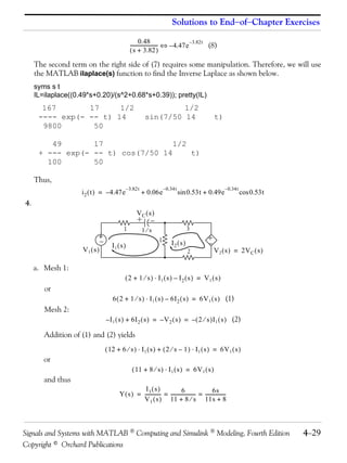


![Chapter 4 Circuit Analysis with Laplace Transforms
8.
1 ⁄ Cs R2
R1 R2 1 ⁄ Cs R1
V in ( s ) V in ( s ) V out ( s )
V out ( s )
(a) (b)
Network (a):
R × 1 ⁄ Cs V (s) z
Let z 1 = R 1 and z 2 = R 2 || 1 ⁄ Cs = ------------------------- . For inverting op amps ----------------- = – ---- , and
2
- out
- 2
-
R 2 + 1 ⁄ Cs V in ( s ) z1
thus
V out ( s ) – [ ( R 2 × 1 ⁄ Cs ) ⁄ ( R 2 + 1 ⁄ Cs ) ] – ( R 2 × 1 ⁄ Cs ) –R1 C
G ( s ) = ----------------- = ------------------------------------------------------------------------- = ----------------------------------------- = -------------------------
- - - -
V in ( s ) R1 R 1 ⋅ ( R 2 + 1 ⁄ Cs ) s + 1 ⁄ R2 C
This network is a first−order active low−pass filter.
Network (b):
V (s) z
Let z 1 = R 1 + 1 ⁄ Cs and z 2 = R 2 . For inverting op-amps ----------------- = – ---- , and thus
out
- 2
-
V in ( s ) z1
V out ( s ) –R2 – ( R 2 ⁄ R 1 )s
G ( s ) = ----------------- = ------------------------- = --------------------------
- - -
V in ( s ) R 1 + 1 ⁄ Cs s + 1 ⁄ R1 C
This network is a first−order active high−pass filter.
4−32 Signals and Systems with MATLAB Computing and Simulink Modeling, Fourth Edition
Copyright © Orchard Publications](https://image.slidesharecdn.com/signalsandsystemswithmatlabcomputingandsimulinkmodeling-121109110233-phpapp02/85/Signals-and-systems-with-matlab-computing-and-simulink-modeling-135-320.jpg)


![Solution of Single State Equations
We will now prove that the solution of the first state equation in (5.22) is
α ( t – t0 ) t
αt – ατ
x(t) = e x0 + e ∫t e
0
β u ( τ ) dτ (5.24)
Proof:
First, we must show that (5.24) satisfies the initial condition of (5.23). This is done by substitu-
tion of t = t0 in (5.24). Then,
t0
α ( t0 – t0 ) αt –α τ
x ( t0 ) = e x0 + e ∫t 0
e β u ( τ ) dτ (5.25)
The first term in the right side of (5.25) reduces to x 0 since
α ( t0 – t0 )
e x0 = e x0 = x0
0
(5.26)
The second term of (5.25) is zero since the upper and lower limits of integration are the same.
Therefore, (5.25) reduces to x ( t 0 ) = x 0 and thus the initial condition is satisfied.
Next, we must prove that (5.24) satisfies also the first equation in (5.22). To prove this, we dif-
ferentiate (5.24) with respect to t and we obtain
d- α ( t – t0 ) d- αt t
– ατ
x ( t ) = ---- ( e
·
dt
x 0 ) + ---- e
dt ∫t e 0
β u ( τ ) dτ
or t
α ( t – t0 ) αt – ατ αt – ατ
x(t) = αe
· x0 + α e ∫t 0
e β u ( τ ) dτ + e [ e βu(τ)] τ = t
α ( t – t0 ) t
αt – ατ αt – αt
= α e x0 + e ∫t 0
e β u ( τ ) dτ + e e βu(t)
or
α ( t – t0 ) t
α(t – τ)
x(t)= α e
· x0 + ∫t e
0
β u ( τ ) dτ + β u ( t ) (5.27)
We observe that the bracketed terms of (5.27) are the same as the right side of the assumed solu-
tion of (5.24). Therefore,
·
x = αx + βu
and this is the same as the first equation of (5.22).
In summary, if α and β are scalar constants, the solution of
·
x = αx + βu (5.28)
Signals and Systems with MATLAB Computing and Simulink Modeling, Fourth Edition 5−7
Copyright © Orchard Publications](https://image.slidesharecdn.com/signalsandsystemswithmatlabcomputingandsimulinkmodeling-121109110233-phpapp02/85/Signals-and-systems-with-matlab-computing-and-simulink-modeling-145-320.jpg)
![Chapter 5 State Variables and State Equations
with initial condition
x0 = x ( t0 ) (5.29)
is obtained from the relation
α ( t – t0 ) t
αt –α τ
x(t) = e x0 + e ∫t e
0
β u ( τ ) dτ (5.30)
Example 5.5
Use (5.28) through (5.30) to find the capacitor voltage v C ( t ) of the circuit of Figure 5.6 for t > 0 ,
given that the initial condition is v C ( 0 − ) = 1 V
R
2Ω C +
+ vC ( t )
−
2u 0 ( t ) 0.5 F −
Figure 5.6. Circuit for Example 5.5
Solution:
From (5.20) of Example 5.3, Page 5−5,
1
x = – ------- x + v S u 0 ( t )
· -
RC
and by comparison with (5.28),
1 –1
α = – ------- = ---------------- = – 1
-
RC 2 × 0.5
and
β = 2
Then, from (5.30),
α ( t – t0 ) t t
αt –α τ –1 ( t – 0 ) –t τ
x(t) = e x0 + e ∫t 0
e β u ( τ ) dτ = e 1+e ∫0 e 2u ( τ ) dτ
t t
–t –t τ –t –t τ –t –t
∫0
t
= e + 2e e dτ = e + 2e [ e ] 0
= e + 2e ( e – 1 )
or
–t
v C ( t ) = x ( t ) = ( 2 – e )u 0 ( t ) (5.31)
Assuming that the output y is the capacitor voltage, the output state equation is
5− 8 Signals and Systems with MATLAB Computing and Simulink Modeling, Fourth Edition
Copyright © Orchard Publications](https://image.slidesharecdn.com/signalsandsystemswithmatlabcomputingandsimulinkmodeling-121109110233-phpapp02/85/Signals-and-systems-with-matlab-computing-and-simulink-modeling-146-320.jpg)


![Computation of the State Transition Matrix
5.4 Computation of the State Transition Matrix e
At
Let A be an n × n matrix, and I be the n × n identity matrix. By definition, the eigenvalues λ i ,
i = 1, 2, …, n of A are the roots of the nth order polynomial
det [ A – λI ] = 0 (5.46)
We recall that expansion of a determinant produces a polynomial. The roots of the polynomial of
(5.46) can be real (unequal or equal), or complex numbers.
Evaluation of the state transition matrix e is based on the Cayley−Hamilton theorem. This theo-
At
rem states that a matrix can be expressed as an ( n – 1 )th degree polynomial in terms of the
matrix A as
At 2 n–1
e = a0 I + a1 A + a2 A + … + an – 1 A (5.47)
where the coefficients a i are functions of the eigenvalues λ .
We accept (5.47) without proving it. The proof can be found in Linear Algebra and Matrix The-
ory textbooks.
Since the coefficients a i are functions of the eigenvalues λ , we must consider the two cases dis-
cussed in Subsections 5.4.1 and 5.4.2 below.
5.4.1 Distinct Eigenvalues (Real of Complex)
If λ 1 ≠ λ 2 ≠ λ 3 ≠ … ≠ λ n , that is, if all eigenvalues of a given matrix A are distinct, the coeffi-
cients a i are found from the simultaneous solution of the following system of equations:
2 n–1 λ1 t
a0 + a1 λ1 + a2 λ1 + … + an – 1 λ1 = e
2 n–1 λ2 t
a0 + a1 λ2 + a2 λ2 + … + an – 1 λ2 = e
(5.48)
…
2 n–1 λn t
a0 + a1 λn + a2 λn + … + an – 1 λn = e
Example 5.6
Compute the state transition matrix e given that
At
Signals and Systems with MATLAB Computing and Simulink Modeling, Fourth Edition 5−11
Copyright © Orchard Publications](https://image.slidesharecdn.com/signalsandsystemswithmatlabcomputingandsimulinkmodeling-121109110233-phpapp02/85/Signals-and-systems-with-matlab-computing-and-simulink-modeling-149-320.jpg)
![Chapter 5 State Variables and State Equations
A = –2 1
0 –1
Solution:
We must first find the eigenvalues λ of the given matrix A . These are found from the expansion
of
det [ A – λI ] = 0
For this example,
det [ A – λI ] = det – 2 1 – λ 1 0 = det – 2 – λ 1 = 0
0 –1 0 1 0 –1–λ
= (– 2 – λ)(– 1 – λ) = 0
or
(λ + 1 )( λ + 2) = 0
Therefore,
λ 1 = – 1 and λ 2 = – 2 (5.49)
Next, we must find the coefficients a i of (5.47). Since A is a 2 × 2 matrix, we only need to con-
sider the first two terms of that relation, that is,
At
e = a0 I + a1 A (5.50)
The coefficients a 0 and a 1 are found from (5.48). For this example,
λ1 t
a0 + a1 λ1 = e
λ2 t
a0 + a1 λ2 = e
or
–t
a0 + a1 ( –1 ) = e
(5.51)
– 2t
a0 + a1 ( –2 ) = e
Simultaneous solution of (5.51) yields
–t – 2t
a 0 = 2e – e
(5.52)
–t – 2t
a1 = e – e
and by substitution into (5.50),
) –2 1
At –t – 2t 1 0 –t – 2t
e = ( 2e – e ) + (e – e
0 1 0 –1
5−12 Signals and Systems with MATLAB Computing and Simulink Modeling, Fourth Edition
Copyright © Orchard Publications](https://image.slidesharecdn.com/signalsandsystemswithmatlabcomputingandsimulinkmodeling-121109110233-phpapp02/85/Signals-and-systems-with-matlab-computing-and-simulink-modeling-150-320.jpg)
![Computation of the State Transition Matrix
or
– 2t –t – 2t
e
At
= e e –e (5.53)
–t
0 e
In summary, we compute the state transition matrix e for a given matrix A using the following
At
procedure:
1. We find the eigenvalues λ from det [ A – λI ] = 0 . We can write [ A – λI ] at once by sub-
tracting λ from each of the main diagonal elements of A . If the dimension of A is a 2 × 2
matrix, it will yield two eigenvalues; if it is a 3 × 3 matrix, it will yield three eigenvalues, and
so on. If the eigenvalues are distinct, we perform steps 2 through 4; otherwise we refer to Sub-
section 5.4.2 below.
2. If the dimension of A is a 2 × 2 matrix, we use only the first 2 terms of the right side of the
state transition matrix
At 2 n–1
e = a0 I + a1 A + a2 A + … + an – 1 A (5.54)
If A matrix is a 3 × 3 matrix, we use the first 3 terms of (5.54), and so on.
3. We obtain the a i coefficients from
2 n–1 λ1 t
a0 + a1 λ1 + a2 λ1 + … + an – 1 λ1 = e
2 n–1 λ2 t
a0 + a1 λ2 + a2 λ2 + … + an – 1 λ2 = e
…
2 n–1 λn t
a0 + a1 λn + a2 λn + … + an – 1 λn = e
We use as many equations as the number of the eigenvalues, and we solve for the coefficients
ai .
4. We substitute the a i coefficients into the state transition matrix of (5.54), and we simplify.
Example 5.7
Compute the state transition matrix e given that
At
Signals and Systems with MATLAB Computing and Simulink Modeling, Fourth Edition 5−13
Copyright © Orchard Publications](https://image.slidesharecdn.com/signalsandsystemswithmatlabcomputingandsimulinkmodeling-121109110233-phpapp02/85/Signals-and-systems-with-matlab-computing-and-simulink-modeling-151-320.jpg)
![Chapter 5 State Variables and State Equations
5 7 –5
A = 0 4 –1 (5.55)
2 8 –3
Solution:
1. We first compute the eigenvalues from det [ A – λI ] = 0 . We obtain [ A – λI ] at once, by sub-
tracting λ from each of the main diagonal elements of A . Then,
5–λ 7 –5
det [ A – λI ] = det 0 4–λ –1 = 0 (5.56)
2 8 –3–λ
and expansion of this determinant yields the polynomial
3 2
λ – 6λ + 11λ – 6 = 0 (5.57)
We will use MATLAB roots(p) function to obtain the roots of (5.57).
p=[1 −6 11 −6]; r=roots(p); fprintf(' n'); fprintf('lambda1 = %5.2f t', r(1));...
fprintf('lambda2 = %5.2f t', r(2)); fprintf('lambda3 = %5.2f', r(3))
lambda1 = 3.00 lambda2 = 2.00 lambda3 = 1.00
and thus the eigenvalues are
λ1 = 1 λ2 = 2 λ3 = 3 (5.58)
2. Since A is a 3 × 3 matrix, we use the first 3 terms of (5.54), that is,
At 2
e = a0 I + a1 A + a2 A (5.59)
3. We obtain the coefficients a 0, a 1, and a 2 from
2 λ1 t
a0 + a1 λ1 + a2 λ1 = e
2 λ2 t
a0 + a1 λ2 + a2 λ2 = e
2 λ3 t
a0 + a1 λ3 + a2 λ3 = e
or
t
a0 + a1 + a2 = e
a 0 + 2a 1 + 4a 2 = e
2t
(5.60)
3t
a 0 + 3a 1 + 9a 2 = e
5−14 Signals and Systems with MATLAB Computing and Simulink Modeling, Fourth Edition
Copyright © Orchard Publications](https://image.slidesharecdn.com/signalsandsystemswithmatlabcomputingandsimulinkmodeling-121109110233-phpapp02/85/Signals-and-systems-with-matlab-computing-and-simulink-modeling-152-320.jpg)
![Computation of the State Transition Matrix
We will use the following MATLAB script for the solution of (5.60).
B=sym('[1 1 1; 1 2 4; 1 3 9]'); b=sym('[exp(t); exp(2*t); exp(3*t)]'); a=Bb; fprintf(' n');...
disp('a0 = '); disp(a(1)); disp('a1 = '); disp(a(2)); disp('a2 = '); disp(a(3))
a0 =
3*exp(t)-3*exp(2*t)+exp(3*t)
a1 =
-5/2*exp(t)+4*exp(2*t)-3/2*exp(3*t)
a2 =
1/2*exp(t)-exp(2*t)+1/2*exp(3*t)
Thus, t 2t 3t
a 0 = 3e – 3e + e
5 t 2t 3 3t
a 1 = – -- e + 4e – -- e
- - (5.61)
2 2
1 t 2t 1 3t
a 2 = -- e – e + -- e
- -
2 2
4. We also use MATLAB to perform the substitution into the state transition matrix, and to per-
form the matrix multiplications. The script is shown below.
syms t; a0 = 3*exp(t)+exp(3*t)−3*exp(2*t); a1 = −5/2*exp(t)−3/2*exp(3*t)+4*exp(2*t);...
a2 = 1/2*exp(t)+1/2*exp(3*t)−exp(2*t);...
A = [5 7 −5; 0 4 −1; 2 8 -3]; eAt=a0*eye(3)+a1*A+a2*A^2
eAt =
[-2*exp(t)+2*exp(2*t)+exp(3*t), -6*exp(t)+5*exp(2*t)+exp(3*t),
4*exp(t)-3*exp(2*t)-exp(3*t)]
[-exp(t)+2*exp(2*t)-exp(3*t), -3*exp(t)+5*exp(2*t)-exp(3*t),
2*exp(t)-3*exp(2*t)+exp(3*t)]
[-3*exp(t)+4*exp(2*t)-exp(3*t), -9*exp(t)+10*exp(2*t)-exp(3*t),
6*exp(t)-6*exp(2*t)+exp(3*t)]
Thus,
t 2t 3t t 2t 3t t 2t 3t
– 2e + 2e + e – 6 e + 5e + e 4e – 3e – e
At
e = t 2t
– e + 2e – e
3t t 2t
– 3e + 5e – e
3t t 2t
2e – 3e + e
3t
t 2t 3t t 2t 3t t 2t 3t
– 3e + 4e – e – 9e + 10e – e 6e – 6e + e
5.4.2 Multiple (Repeated) Eigenvalues
In this case, we will assume that the polynomial of
det [ A – λI ] = 0 (5.62)
Signals and Systems with MATLAB Computing and Simulink Modeling, Fourth Edition 5−15
Copyright © Orchard Publications](https://image.slidesharecdn.com/signalsandsystemswithmatlabcomputingandsimulinkmodeling-121109110233-phpapp02/85/Signals-and-systems-with-matlab-computing-and-simulink-modeling-153-320.jpg)
![Chapter 5 State Variables and State Equations
has n roots, and m of these roots are equal. In other words, the roots are
λ1 = λ2 = λ3 … = λm , λm + 1 , λn (5.63)
The coefficients a i of the state transition matrix
At n–1
= a0 I + a1 A + a2 A + … + an – 1 A (5.64)
2
e
are found from the simultaneous solution of the system of equations of (5.65) below.
n–1 λ1 t
a0 + a1 λ1 + a2 λ1 + … + an – 1 λ1
2
= e
d- d- λ t
-------- ( a 0 + a 1 λ 1 + a 2 λ 2 + … + a n – 1 λ n – 1 ) = ------- e 1
1 1
dλ 1 dλ 1
2 2
d d λt
-------2 ( a 0 + a 1 λ 1 + a 2 λ 2 + … + a n – 1 λ n – 1 ) = -------2 e 1
- 1 1 -
dλ 1 dλ 1
… (5.65)
m–1 m–1
d d λ t
-------------- ( a 0 + a 1 λ 1 + a 2 λ 2 + … + a n – 1 λ n – 1 ) = -------------- e 1
m–1
- 1 1 m–1
-
dλ 1 dλ 1
n–1 λ m + 1t
a0 + a1 λm + 1 + a2 λm + 1 + … + an – 1 λm + 1 = e
2
…
n–1 λn t
a 0 + a 1 λn + a 2 λ n + … + a n – 1 λ n
2
= e
Example 5.8
Compute the state transition matrix e given that
At
A = –1 0
2 –1
Solution:
1. We first find the eigenvalues λ of the matrix A and these are found from the polynomial of
det [ A – λI ] = 0 . For this example,
det [ A – λI ] = det – 1 – λ 0 = 0 2
(– 1 – λ)(– 1 – λ) = 0 (λ + 1) = 0
2 –1–λ
and thus,
5−16 Signals and Systems with MATLAB Computing and Simulink Modeling, Fourth Edition
Copyright © Orchard Publications](https://image.slidesharecdn.com/signalsandsystemswithmatlabcomputingandsimulinkmodeling-121109110233-phpapp02/85/Signals-and-systems-with-matlab-computing-and-simulink-modeling-154-320.jpg)

![Chapter 5 State Variables and State Equations
We will first use MATLAB to verify the values of the eigenvalues found in Examples 5.6 through
5.8, and we will briefly discuss eigenvectors in the next section.
Example 5.6:
A= [−2 1; 0 −1]; lambda=eig(A)
lambda =
-2
-1
Example 5.7:
B = [5 7 −5; 0 4 −1; 2 8 −3]; lambda=eig(B)
lambda =
1.0000
3.0000
2.0000
Example 5.8:
C = [−1 0; 2 −1]; lambda=eig(C)
lambda =
-1
-1
5.5 Eigenvectors
Consider the relation
AX = λX (5.69)
where A is an n × n matrix, X is a column vector, and λ is a scalar number. We can express this
relation in matrix form as
a 11 a 12 … a 1n x 1 x1
a 21 a 22 … a 2n x 2 x2
= λ (5.70)
… … … … … …
a n1 a n2 … a nn x n xn
We write (5.70) as
( A – λI )X = 0 (5.71)
Then, (5.71) can be written as
5−18 Signals and Systems with MATLAB Computing and Simulink Modeling, Fourth Edition
Copyright © Orchard Publications](https://image.slidesharecdn.com/signalsandsystemswithmatlabcomputingandsimulinkmodeling-121109110233-phpapp02/85/Signals-and-systems-with-matlab-computing-and-simulink-modeling-156-320.jpg)


![Chapter 5 State Variables and State Equations
We will compute the solution of (5.88) using
A ( t – t0 ) t
–A τ
∫t e
At
x( t) = e x0 + e bu ( τ ) dτ (5.89)
0
where
–4 –4 iL ( 0 ) 0
A = x0 = = b = 4 (5.90)
3⁄4 0 vC ( 0 ) 1⁄2 0
First, we compute the state transition matrix e . We find the eigenvalues from
At
det [ A – λI ] = 0
Then,
det [ A – λI ] = det – 4 – λ – 4 = 0
2
( –λ ) ( – 4 – λ ) + 3 = 0 λ + 4λ + 3 = 0
3 ⁄ 4 –λ
Therefore,
λ 1 = – 1 and λ 2 = – 3
The next step is to find the coefficients a i . Since A is a 2 × 2 matrix, we only need the first two
terms of the state transition matrix, that is,
At
e = a0 I + a1 A (5.91)
The constants a 0 and a 1 are found from
λ1 t
a0 + a1 λ1 = e
λ2 t
a0 + a1 λ2 = e
and with λ 1 = – 1 and λ 2 = – 3 , we obtain
–t
a0 –a1 = e
(5.92)
– 3t
a 0 – 3a 1 = e
Simultaneous solution of (5.92) yields
–t – 3t
a 0 = 1.5e – 0.5e
(5.93)
–t – 3t
a 1 = 0.5e – 0.5e
We now substitute these values into (5.91), and we obtain
5−24 Signals and Systems with MATLAB Computing and Simulink Modeling, Fourth Edition
Copyright © Orchard Publications](https://image.slidesharecdn.com/signalsandsystemswithmatlabcomputingandsimulinkmodeling-121109110233-phpapp02/85/Signals-and-systems-with-matlab-computing-and-simulink-modeling-162-320.jpg)


![Circuit Analysis with State Variables
1
0.9
0.8
0.7
0.6
0.5
0 1 2 3 4 5 6 7 8 9 10
Figure 5.8. Plot for relation (5.97)
We can obtain the plot of Figure 5.8 with the Simulink State−Space block with the unit step
function as the input using the Step block, and the capacitor voltage as the output displayed on
the Scope block as shown in the model of Figure 5.9 where for the State−Space block Function
Block Parameters dialog box we have entered:
A: [−4 −4; 3/4 0]
B: [4 0]’
C: [0 1]
D: [ 0 ]
Initial conditions: [0 1/2]
Figure 5.9. Simulink model for Example 5.10
The waveform for the capacitor voltage for the simulation time interval 0 ≤ t ≤ 10 seconds is
shown in Figure 5.10 where we observe that the initial condition v C ( 0 − ) = 0.5 V is also dis-
played.
Signals and Systems with MATLAB Computing and Simulink Modeling, Fourth Edition 5−27
Copyright © Orchard Publications](https://image.slidesharecdn.com/signalsandsystemswithmatlabcomputingandsimulinkmodeling-121109110233-phpapp02/85/Signals-and-systems-with-matlab-computing-and-simulink-modeling-165-320.jpg)
![Chapter 5 State Variables and State Equations
Figure 5.10. Input and output waveforms for the model of Figure 5.9
Example 5.11
A network is described by the state equation
·
x = Ax + bu (5.98)
where
A = 1 0 x0 = 1 b = –1 and u = δ ( t ) (5.99)
1 –1 0 1
Compute the state vector
x1
x =
x2
Solution:
We compute the eigenvalues from
det [ A – λI ] = 0
For this example,
det [ A – λI ] = det 1 – λ 0 = 0 ( 1 –λ ) ( – 1 – λ ) = 0
1 –1 –λ
Then,
λ 1 = 1 and λ 2 = – 1
Since A is a 2 × 2 matrix, we only need the first two terms of the state transition matrix to find
the coefficients a i , that is,
At
e = a0 I + a1 A (5.100)
The constants a 0 and a 1 are found from
5−28 Signals and Systems with MATLAB Computing and Simulink Modeling, Fourth Edition
Copyright © Orchard Publications](https://image.slidesharecdn.com/signalsandsystemswithmatlabcomputingandsimulinkmodeling-121109110233-phpapp02/85/Signals-and-systems-with-matlab-computing-and-simulink-modeling-166-320.jpg)

![Chapter 5 State Variables and State Equations
5.7 Relationship between State Equations and Laplace Transform
In this section, we will show that the state transition matrix can be computed from the Inverse
Laplace transform. We will also show that the transfer function can be found from the coefficient
matrices of the state equations.
Consider the state equation
·
x = Ax + bu (5.106)
Taking the Laplace of both sides of (5.106), we obtain
sX ( s ) – x ( 0 ) = AX ( s ) + bU ( s )
or
( sI – A )X ( s ) = x ( 0 ) + bU ( s ) (5.107)
Multiplying both sides of (5.107) by ( sI – A ) –1 , we obtain
–1 –1
X ( s ) = ( sI – A ) x ( 0 ) + ( sI – A ) bU ( s ) (5.108)
Comparing (5.108) with
t
–A τ
∫0 e
At At
x ( t ) = e x0 + e bu ( τ ) dτ (5.109)
we observe that the right side of (5.108) is the Laplace transform of (5.109). Therefore, we can
compute the state transition matrix e from the Inverse Laplace of ( sI – A ) –1 , that is, we can use
At
the relation
At –1 –1
e = L { ( sI – A ) } (5.110)
Next, we consider the output state equation
y = Cx + du (5.111)
Taking the Laplace of both sides of (5.111), we obtain
Y ( s ) = CX ( s ) + dU ( s ) (5.112)
and using (5.108), we obtain
–1 –1
Y ( s ) = C ( sI – A ) x ( 0 ) + [ C ( sI – A ) b + d ]U ( s ) (5.113)
If the initial condition x ( 0 ) = 0 , (5.113) reduces to
–1
Y ( s ) = [ C ( sI – A ) b + d ]U ( s ) (5.114)
5−30 Signals and Systems with MATLAB Computing and Simulink Modeling, Fourth Edition
Copyright © Orchard Publications](https://image.slidesharecdn.com/signalsandsystemswithmatlabcomputingandsimulinkmodeling-121109110233-phpapp02/85/Signals-and-systems-with-matlab-computing-and-simulink-modeling-168-320.jpg)


![Relationship between State Equations and Laplace Transform
t
–A τ
∫0 e
At At
x ( t ) = e x0 + e bu ( τ ) dτ
using the procedure of Example 5.11.
MATLAB provides two very useful functions to convert state−space (state equations), to trans-
fer function (s−domain), and vice versa. The function ss2tf (state−space to transfer function)
converts the state space equations
·
x = Ax + Bu *
(5.124)
y = Cx + Du
to the rational transfer function form
N(s)
G ( s ) = ----------- (5.125)
D(s)
This is used with the statement [num,den]=ss2tf(A,B,C,D,iu) where A, B, C, D are the matrices
of (5.124) and iu is 1 if there is only one input. The MATLAB help command provides the fol-
lowing information:
help ss2tf
SS2TF State-space to transfer function conversion.
[NUM,DEN] = SS2TF(A,B,C,D,iu) calculates the
transfer function:
NUM(s) -1
G(s) = -------- = C(sI-A) B + D
DEN(s)
of the system:
x = Ax + Bu
y = Cx + Du
from the iu'th input. Vector DEN contains the coefficients of the
denominator in descending powers of s. The numerator coefficients are
returned in matrix NUM with as many rows as there are outputs y.
See also TF2SS
The other function, tf2ss, converts the transfer function of (5.125) to the state−space equations
of (5.124). It is used with the statement [A,B,C,D]=tf2ss(num,den) where A, B, C, and D are
the matrices of (5.124), and num, den are N ( s ) and D ( s ) of (5.125) respectively. The MATLAB
help command provides the following information:
* We have used capital letters for vectors b and c to be consistent with MATLAB’s designations.
Signals and Systems with MATLAB Computing and Simulink Modeling, Fourth Edition 5−33
Copyright © Orchard Publications](https://image.slidesharecdn.com/signalsandsystemswithmatlabcomputingandsimulinkmodeling-121109110233-phpapp02/85/Signals-and-systems-with-matlab-computing-and-simulink-modeling-171-320.jpg)
![Chapter 5 State Variables and State Equations
help tf2ss
TF2SS Transfer function to state-space conversion.
[A,B,C,D] = TF2SS(NUM,DEN) calculates the state-space
representation:
x = Ax + Bu
y = Cx + Du
of the system:
NUM(s)
G(s) = --------
DEN(s)
from a single input. Vector DEN must contain the coefficients of the
denominator in descending powers of s. Matrix NUM must contain the
numerator coefficients with as many rows as there are outputs y. The
A,B,C,D matrices are returned in controller canonical form. This calcu-
lation also works for discrete systems. To avoid confusion when using
this function with discrete systems, always use a numerator polynomial
that has been padded with zeros to make it the same length as the denom-
inator. See the User's guide for more details.
See also SS2TF.
Example 5.13
For the circuit of Figure 5.12, all initial conditions are zero.
R L
1Ω 1H
C +
+ v C ( t ) = v out ( t )
− i( t) −
1F
vS ( t ) = u0 ( t )
Figure 5.12. Circuit for Example 5.13
a. Derive the state equations and express them in matrix form as
·
x = Ax + Bu
y = Cx + Du
b. Derive the transfer function
N(s)
G ( s ) = -----------
D(s)
c. Verify your answers with MATLAB.
5−34 Signals and Systems with MATLAB Computing and Simulink Modeling, Fourth Edition
Copyright © Orchard Publications](https://image.slidesharecdn.com/signalsandsystemswithmatlabcomputingandsimulinkmodeling-121109110233-phpapp02/85/Signals-and-systems-with-matlab-computing-and-simulink-modeling-172-320.jpg)
![Chapter 5 State Variables and State Equations
R L
1Ω s
+
C +
V C ( s ) = V out ( s )
− 1⁄s −
V in ( s )
Figure 5.13. Transformed circuit for Example 5.13
By the voltage division expression,
1⁄s -
V out ( s ) = -------------------------- V in ( s )
1+s+1⁄s
or
V out ( s ) 1 -
----------------- = ---------------------
-
V in ( s ) 2
s +s+1
Therefore,
V out ( s ) 1 -
G ( s ) = ----------------- = ---------------------
- (5.127)
V in ( s ) 2
s +s+1
c.
A = [−1 −1; 1 0]; B = [1 0]'; C = [0 1]; D = [0]; % The matrices of (5.126)
[num, den] = ss2tf(A, B, C, D, 1) % Verify coefficients of G(s) in (5.127)
num =
0 0 1
den =
1.0000 1.0000 1.0000
num = [0 0 1]; den = [1 1 1]; % The coefficients of G(s) in (5.127)
[A B C D] = tf2ss(num, den) % Verify the matrices of (5.126)
A =
-1 -1
1 0
B =
1
0
C =
0 1
D =
0
The equivalence between the state−space equations of (5.126) and the transfer function of
(5.127) is also evident from the Simulink models shown in Figure 5.14 where for the State−
Space block Function Block Parameters dialog box we have entered:
5−36 Signals and Systems with MATLAB Computing and Simulink Modeling, Fourth Edition
Copyright © Orchard Publications](https://image.slidesharecdn.com/signalsandsystemswithmatlabcomputingandsimulinkmodeling-121109110233-phpapp02/85/Signals-and-systems-with-matlab-computing-and-simulink-modeling-174-320.jpg)
![Relationship between State Equations and Laplace Transform
A: [−1 −1; 3/4 0]
B: [1 0]’
C: [0 1]
D: [ 0 ]
Initial conditions: [0 0]
For the Transfer Fcn block Function Block Parameters dialog box we have entered:
Numerator coefficient: [ 1 ]
Denominator coefficient: [1 1 1]
Figure 5.14. Models to show the equivalence between relations (5.126) and (5.127)
After the simulation command is executed, both Scope 1 and Scope 2 blocks display the input
and output waveforms shown in Figure 5.15.
Figure 5.15. Waveforms displayed by Scope 1 and Scope 2 blocks for the models in Figure 5.14
Signals and Systems with MATLAB Computing and Simulink Modeling, Fourth Edition 5−37
Copyright © Orchard Publications](https://image.slidesharecdn.com/signalsandsystemswithmatlabcomputingandsimulinkmodeling-121109110233-phpapp02/85/Signals-and-systems-with-matlab-computing-and-simulink-modeling-175-320.jpg)
![Chapter 5 State Variables and State Equations
5.8 Summary
• An nth−order differential equation can be resolved to n first−order simultaneous differential
equations with a set of auxiliary variables called state variables. The resulting first−order differ-
ential equations are called state−space equations, or simply state equations.
• The state−space equations can be obtained either from the nth−order differential equation, or
directly from the network, provided that the state variables are chosen appropriately.
• When we obtain the state equations directly from given circuits, we choose the state variables
to represent inductor currents and capacitor voltages.
• The state variable method offers the advantage that it can also be used with non−linear and
time−varying devices.
• If a circuit contains only one energy−storing device, the state equations are written as
·
x = αx + βu
y = k1 x + k2 u
where α , β , k 1 , and k 2 are scalar constants, and the initial condition, if non−zero, is denoted
as
x0 = x ( t0 )
• If α and β are scalar constants, the solution of x = α x + β u with initial condition x 0 = x ( t 0 )
·
is obtained from the relation
α ( t – t0 ) t
αt –α τ
x( t) = e x0 + e ∫t e
0
β u ( τ ) dτ
• The solution of the state equations pair
·
x = Ax + bu
y = Cx + du
where A and C are 2 × 2 or higher order matrices, and b and d are column vectors with two
or more rows, entails the computation of the state transition matrix e , and integration of
At
A ( t – t0 ) t
–A τ
∫t e
At
x(t) = e x0 + e bu ( τ ) dτ
0
• The eigenvalues λ i , where i = 1, 2, …, n , of an n × n matrix A are the roots of the nth order
polynomial
det [ A – λI ] = 0
where I is the n × n identity matrix.
5−38 Signals and Systems with MATLAB Computing and Simulink Modeling, Fourth Edition
Copyright © Orchard Publications](https://image.slidesharecdn.com/signalsandsystemswithmatlabcomputingandsimulinkmodeling-121109110233-phpapp02/85/Signals-and-systems-with-matlab-computing-and-simulink-modeling-176-320.jpg)


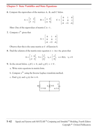


![Solutions to End−of−Chapter Exercises
di L
v C1 = L ------- + v C2
dt
or ·
x 2 = 1x 1 + x 3
or ·
x 1 = x 2 – x 3 (2)
Also,
dv C2
i L = C -----------
-
dt
or ·
x 1 = 2x 3
or
· 1
x 3 = -- x 1 (3)
-
2
Combining (1), (2), and (3) into matrix form we obtain
·
x1 0 1 –1 x1 0
– 1 ⁄ 2 – 1 ⁄ 2 0 ⋅ x 2 + 1 ⁄ 2 ⋅ V p cos ωtu 0 ( t )
· =
x2
· 1⁄2 0 0 x3 0
x3
We will create a Simulink model with V p = 1 and output y = x 3 . The model is shown below
where for the State−Space block Function Block Parameters dialog box we have entered:
A: [0 1 −1; −1/2 −1/2 0; 1/2 0 0]
B: [0 1/2 0]’
C: [0 0 1]
D: [ 0 ]
Initial conditions: [0 0 0]
and for the Sine Wave block Function Block Parameters dialog box we have entered:
Amplitude: 1
Phase: pi/2
The input and output waveforms are shown below.
Signals and Systems with MATLAB Computing and Simulink Modeling, Fourth Edition 5−45
Copyright © Orchard Publications](https://image.slidesharecdn.com/signalsandsystemswithmatlabcomputingandsimulinkmodeling-121109110233-phpapp02/85/Signals-and-systems-with-matlab-computing-and-simulink-modeling-183-320.jpg)


![Chapter 5 State Variables and State Equations
2 λ1 t –t
a0 + a1 λ1 + a2 λ1 = e ⇒ a0 – a1 + a2 = e
2 λ2 t – 2t
a0 + a1 λ2 + a2 λ2 = e ⇒ a 0 – 2a 1 + 4a 2 = e
2 λ3 t – 3t
a0 + a1 λ3 + a2 λ3 = e ⇒ a 0 – 3a 1 + 9a 2 = e
syms t; A=[1 −1 1; 1 −2 4; 1 −3 9];...
a=sym('[exp(−t); exp(−2*t); exp(−3*t)]'); x=Aa; fprintf(' n');...
disp('a0 = '); disp(x(1)); disp('a1 = '); disp(x(2)); disp('a2 = '); disp(x(3))
a0 =
3*exp(-t)-3*exp(-2*t)+exp(-3*t)
a1 =
5/2*exp(-t)-4*exp(-2*t)+3/2*exp(-3*t)
a2 =
1/2*exp(-t)-exp(-2*t)+1/2*exp(-3*t)
Thus,
–t – 2t – 3t
a 0 = 3e – 3e + 3e
–t – 2t – 3t
a 1 = 2.5e – 4e + 1.5e
–t – 2t – 3t
a 2 = 0.5e – e + 0.5e
Now, we compute e of (1) with the following MATLAB script:
At
syms t; a0=3*exp(−t)−3*exp(−2*t)+exp(−3*t); a1=5/2*exp(−t)−4*exp(−2*t)+3/2*exp(−3*t);...
a2=1/2*exp(−t)-exp(−2*t)+1/2*exp(−3*t); A=[0 1 0; 0 0 1; −6 −11 −6]; fprintf(' n');...
eAt=a0*eye(3)+a1*A+a2*A^2
eAt =
[3*exp(-t)-3*exp(-2*t)+exp(-3*t), 5/2*exp(-t)-4*exp(-2*t)+3/
2*exp(-3*t), 1/2*exp(-t)-exp(-2*t)+1/2*exp(-3*t)]
[-3*exp(-t)+6*exp(-2*t)-3*exp(-3*t), -5/2*exp(-t)+8*exp(-2*t)-
9/2*exp(-3*t), -1/2*exp(-t)+2*exp(-2*t)-3/2*exp(-3*t)]
[3*exp(-t)-12*exp(-2*t)+9*exp(-3*t), 5/2*exp(-t)-16*exp(-
2*t)+27/2*exp(-3*t), 1/2*exp(-t)-4*exp(-2*t)+9/2*exp(-3*t)]
Thus,
–t – 2t – 3t –t – 2t – 3t –t – 2t – 3t
3e – 3e +e 2.5e – 4e + 1.5e 0.5e – e + 0.5e
At
e = – 3 e –t + 6e –2t – 3e –3t –t
– 2.5 e + 8e
– 2t
– 4.5e
– 3t –t
– 0.5 e + 2e
– 2t
– 1.5e
– 3t
–t – 2t – 3t –t – 2t – 3t –t – 2t – 3t
3e – 12e + 9e 2.5e – 16e + 13.5e 0.5e – 4e + 4.5e
5−48 Signals and Systems with MATLAB Computing and Simulink Modeling, Fourth Edition
Copyright © Orchard Publications](https://image.slidesharecdn.com/signalsandsystemswithmatlabcomputingandsimulinkmodeling-121109110233-phpapp02/85/Signals-and-systems-with-matlab-computing-and-simulink-modeling-186-320.jpg)
![Solutions to End−of−Chapter Exercises
8.
A= 1 0 , b= 1 , x0 = –1 , u = δ ( t ), t0 = 0
–2 2 2 0
t t
A(t – 0) –A τ –A τ
∫0 ∫0 e
At At At
x( t) = e x0 + e e bu ( τ ) dτ = e x 0 + e bδ ( τ ) dτ
(1)
At
= e x0 + e b = e ( x0 + b ) = e –1 + 1 = e 0
At At At At
0 2 2
We use the following MATLAB script to find the eigenvalues λ 1 and λ 2 .
A=[1 0; −2 2]; lambda=eig(A); fprintf(' n');...
fprintf('lambda1 = %4.2f t',lambda(1)); fprintf('lambda2 = %4.2f t',lambda(2))
lambda1 = 2.00 lambda2 = 1.00
Next,
λ1 t t
a0 + a1 λ1 = e ⇒ a0 + a1 = e
λ2 t 2t
a0 + a1 λ2 = e ⇒ a 0 + 2a 1 = e
Then,
t 2t 2t t
a 0 = 2e – e a1 = e – e
and
= a 0 I + a 1 A = ( 2e – e ) 1 0 + ( e – e ) 1 0
At t 2t 2t t
e
0 1 –2 2
t 2t 2t t t
= 2e – e 0 + e –e 0 = e 0
t 2t 2t t 2t t t 2t 2t
0 2e – e – 2e + 2e 2e – 2e 2e – 2e e
By substitution into (1) we obtain
t
0 = e 0 0
⋅ 0 =
At
x( t) = e
t 2t 2t 2t
2 2e – 2e e 2 2e
and thus
2t
x1 = 0 x 2 = 2e
Signals and Systems with MATLAB Computing and Simulink Modeling, Fourth Edition 5−49
Copyright © Orchard Publications](https://image.slidesharecdn.com/signalsandsystemswithmatlabcomputingandsimulinkmodeling-121109110233-phpapp02/85/Signals-and-systems-with-matlab-computing-and-simulink-modeling-187-320.jpg)
![Chapter 5 State Variables and State Equations
9.
−
C
+ C iL ( 0 ) = 0
iR iL i
R L
−v C v ( 0 − ) = 1 V
C
3⁄4 Ω 4 H 4⁄3 F
We let
x1 = iL x2 = vC
Then,
a.
iR + iL + iC = 0
vC vC
----- + i L + C ----- = 0
- -
R dt
x2 4 ·
-------- + x 1 + -- x 2 = 0
- -
3⁄4 3
or
· 3
x 2 = – -- x 1 – x 2 (1)
-
4
Also,
di L ·
v L = v C = L ------- = 4x 1 = x 2
dt
or
· 1
x 1 = -- x (2)
-
4 2
From (1) and (2)
·
x1
= 0 1 ⁄ 4 ⋅ x1
·
x2 –3 ⁄ 4 –1 x2
and thus
A = 0 1⁄4
–3 ⁄ 4 –1
b.
At –1 –1
e = L { [ sI – A ] }
5−50 Signals and Systems with MATLAB Computing and Simulink Modeling, Fourth Edition
Copyright © Orchard Publications](https://image.slidesharecdn.com/signalsandsystemswithmatlabcomputingandsimulinkmodeling-121109110233-phpapp02/85/Signals-and-systems-with-matlab-computing-and-simulink-modeling-188-320.jpg)
![Solutions to End−of−Chapter Exercises
[ sI – A ] = s 0 – 0 1⁄4 = s –1 ⁄ 4
0 s –3 ⁄ 4 –1 3⁄4 s+1
∆ = det [ sI – A ] = det s – 1 ⁄ 4 = s 2 + s + 3 ⁄ 16 = ( s + 1 ⁄ 4 ) ( s + 3 ⁄ 4 )
3⁄4 s+1
adj [ sI – A ] = adj s –1 ⁄ 4 = s+1 1⁄4
3⁄4 s+1 –3 ⁄ 4 s
[ sI – A ]
–1
= -- adj [ sI – A ] = ---------------------------------------------- s + 1
1- 1 - 1⁄4
∆ ( s + 1 ⁄ 4 ) ( s + 3 ⁄ 4 ) –3 ⁄ 4 s
s+1 1⁄4
----------------------------------------------
- ----------------------------------------------
-
= (s + 1 ⁄ 4)(s + 3 ⁄ 4) (s + 1 ⁄ 4)(s + 3 ⁄ 4)
–3 ⁄ 4 s
----------------------------------------------
- -----------------------------------------------
(s + 1 ⁄ 4)(s + 3 ⁄ 4) (s + 1 ⁄ 4)(s + 3 ⁄ 4)
–1 –1
We use MATLAB to find e { [ sI – A ] } with the script below.
At
= L
syms s t
Fs1=(s+1)/(s^2+s+3/16); Fs2=(1/4)/(s^2+s+3/16); Fs3=(−3/4)/(s^2+s+3/16); Fs4=s/
(s^2+s+3/16);...
fprintf(' n'); disp('a11 = '); disp(simple(ilaplace(Fs1))); disp('a12 = '); disp(simple(ila-
place(Fs2)));...
disp('a21 = '); disp(simple(ilaplace(Fs3))); disp('a22 = '); disp(simple(ilaplace(Fs4)))
a11 =
-1/2*exp(-3/4*t)+3/2*exp(-1/4*t)
a12 =
1/2*exp(-1/4*t)-1/2*exp(-3/4*t)
a21 =
-3/2*exp(-1/4*t)+3/2*exp(-3/4*t)
a22 =
3/2*exp(-3/4*t)-1/2*exp(-1/4*t)
Thus,
– 0.25t – 0.75t – 0.25t – 0.75t
e
At
= 1.5e – 0.5e 0.5e – 0.5e
– 0.25t – 0.75t – 0.25t – 0.75t
– 1.5 e + 1.5e – 0.5 e + 1.5e
Signals and Systems with MATLAB Computing and Simulink Modeling, Fourth Edition 5−51
Copyright © Orchard Publications](https://image.slidesharecdn.com/signalsandsystemswithmatlabcomputingandsimulinkmodeling-121109110233-phpapp02/85/Signals-and-systems-with-matlab-computing-and-simulink-modeling-189-320.jpg)


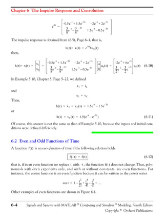

![Chapter 6 The Impulse Response and Convolution
T
∫– T f o ( t ) dt = 0 (6.15)
A function f ( t ) that is neither even nor odd can be expressed as
1
f e ( t ) = -- [ f ( t ) + f ( – t ) ]
- (6.16)
2
or as
1
f o ( t ) = -- [ f ( t ) – f ( – t ) ]
- (6.17)
2
Addition of (6.16) with (6.17) yields
f ( t ) = fe ( t ) + fo ( t ) (6.18)
that is, any function of time can be expressed as the sum of an even and an odd function.
Example 6.3
Determine whether the delta function is an even or an odd function of time.
Solution:
Let f ( t ) be an arbitrary function of time that is continuous at t = t 0 . Then, by the sifting property
of the delta function
∞
∫–∞ f ( t )δ ( t – t ) dt
0 = f ( t0 )
and for t 0 = 0 ,
∞
∫–∞ f ( t )δ ( t ) dt = f(0 )
Also,
∞
∫–∞ fe ( t )δ ( t ) dt = fe ( 0 )
and
∞
∫–∞ fo ( t )δ ( t ) dt = fo ( 0 )
As stated earlier, an odd function f o ( t ) evaluated at t = 0 is zero, that is, f o ( 0 ) = 0 . Therefore,
from the last relation above,
∞
∫–∞ fo ( t )δ ( t ) dt = fo ( 0 ) = 0 (6.19)
6− 6 Signals and Systems with MATLAB ® Computing and Simulink ® Modeling, Fourth Edition
Copyright © Orchard Publications](https://image.slidesharecdn.com/signalsandsystemswithmatlabcomputingandsimulinkmodeling-121109110233-phpapp02/85/Signals-and-systems-with-matlab-computing-and-simulink-modeling-196-320.jpg)


![Chapter 6 The Impulse Response and Convolution
0.5
2
0.4
t ⁄ 2 – 2t + 2
0.3
2
0.2 t–t ⁄2
0.1
0
0 0.2 0.4 0.6 0.8 1 1.2 1.4 1.6 1.8 2
Figure 6.15. Convolution for 0 ≤ τ ≤ 2 of the signals of Example 6.4
The plot of Figure 6.15 was obtained with the MATLAB script below.
t1=0:0.01:1; x=t1−t1.^2./2; axis([0 1 0 0.5]);...
t2=1:0.01:2; y=t2.^2./2−2.*t2+2; axis([1 2 0 0.5]); plot(t1,x,t2,y); grid
Example 6.5
The signals h ( t ) and u ( t ) are as shown in Figure 6.16. Compute h ( t )*u ( t ) using the graphical
evaluation method.
u ( t ) = u0 ( t ) – u0 ( t – 1 )
1 1
–t
h(t) = e
t t
0 0 1
Figure 6.16. Signals for Example 6.5
Solution:
Following the same procedure as in the previous example, we form u ( t – τ ) by first constructing
the image of u ( τ ) . This is shown as u ( – τ ) in Figure 6.17.
u ( –τ )
1
τ
−1 0
Figure 6.17. Construction of u ( – τ ) for Example 6.5
6−12 Signals and Systems with MATLAB ® Computing and Simulink ® Modeling, Fourth Edition
Copyright © Orchard Publications](https://image.slidesharecdn.com/signalsandsystemswithmatlabcomputingandsimulinkmodeling-121109110233-phpapp02/85/Signals-and-systems-with-matlab-computing-and-simulink-modeling-202-320.jpg)


![Graphical Evaluation of the Convolution Integral
u ( t – τ ), t = 1
1
h(τ)
A
τ
0 t−1 t
Figure 6.23. Convolution for interval 1 < t < 2 of Example 6.5
Therefore, for the time interval t > 1 , we have
t t
–τ –τ t –τ t – 1 –( t – 1 )
∫t – 1 ∫t – 1
–t –t
u ( t – τ )h ( τ ) dτ = ( 1 ) ( e ) dτ = – e t–1
= e t
= e –e = e (e – 1)
(6.28)
–t
= 1.732e
Evaluating (6.28) at t = 2 , we find that u ( τ )*h ( τ ) = 0.233 .
For t > 2 , the product u ( t – τ )h ( τ ) approaches zero as t → ∞ . The convolution of these signals for
0 ≤ t ≤ 2 , is shown in Figure 6.24.
0.7
0.6
–t
1–e
–t e (e – 1)
0.5
0.4
0.3
0.2
0.1
0
0 0.2 0.4 0.6 0.8 1 1.2 1.4 1.6 1.8 2
Figure 6.24. Convolution for 0 ≤ t ≤ 2 of the signals of Example 6.5
The plot of Figure 6.24 was obtained with the MATLAB script below.
t1=0:0.01:1; x=1−exp(−t1); axis([0 1 0 0.8]);...
t2=1:0.01:2; y=1.718.*exp(−t2); axis([1 2 0 0.8]); plot(t1,x,t2,y); grid
Example 6.6
Perform the convolution v 1 ( t )*v 2 ( t ) where v 1 ( t ) and v 2 ( t ) are as shown in Figure 6.25.
Signals and Systems with MATLAB ® Computing and Simulink ® Modeling, Fourth Edition 6−15
Copyright © Orchard Publications](https://image.slidesharecdn.com/signalsandsystemswithmatlabcomputingandsimulinkmodeling-121109110233-phpapp02/85/Signals-and-systems-with-matlab-computing-and-simulink-modeling-205-320.jpg)
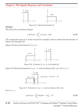


![Summary
6.6 Summary
• The impulse response is the output (voltage or current) of a network when the input is the
delta function.
• The determination of the impulse response assumes zero initial conditions.
• A function f ( t ) is an even function of time if the following relation holds.
f ( –t ) = f ( t )
• A function f ( t ) is an odd function of time if the following relation holds.
–f ( –t ) = f ( t )
• The product of two even or two odd functions is an even function, and the product of an even
function times an odd function, is an odd function.
• A function f ( t ) that is neither even nor odd, can be expressed as
1
f e ( t ) = -- [ f ( t ) + f ( – t ) ]
-
2
or as
1
f o ( t ) = -- [ f ( t ) – f ( – t ) ]
-
2
where f e ( t ) denotes an even function and f o ( t ) denotes an odd function.
• Any function of time can be expressed as the sum of an even and an odd function, that is,
f ( t ) = fe ( t ) + fo ( t )
• The delta function is an even function of time.
• The integral
∞
∫–∞ u ( τ )h ( t – τ ) dτ
or
∞
∫–∞ u ( t – τ )h ( τ ) dτ
is known as the convolution integral.
• If we know the impulse response of a network, we can compute the response to any input u ( t )
with the use of the convolution integral.
Signals and Systems with MATLAB ® Computing and Simulink ® Modeling, Fourth Edition 6−21
Copyright © Orchard Publications](https://image.slidesharecdn.com/signalsandsystemswithmatlabcomputingandsimulinkmodeling-121109110233-phpapp02/85/Signals-and-systems-with-matlab-computing-and-simulink-modeling-211-320.jpg)


![Chapter 6 The Impulse Response and Convolution
∞
u ( t )*h ( t ) = ∫–∞ u ( τ )h ( t – τ ) dτ
where h ( t ) = – t + 1 , h ( τ ) = – τ + 1 , h ( – τ ) = τ + 1 , and h ( t – τ ) = – ( t – τ ) + 1 = 1 – t + τ .
Then, for 0 < t < 1 ,
2 t 2 2
t
τ-
∫ = --- + ( 1 – t )t = t – t -
Area 1 = [ ( 1 – t ) + τ ] dτ = ---- + ( 1 – t )τ t- ---
0 2 0
2 2
and we observe that at t = 1 , Area 1 = 1 ⁄ 2 square units
Next, for 1 < t < 2 ,
2 1
1
Area 2 = [ ( 1 – t ) + τ ] dτ = τ - + ( 1 – t )τ
∫ ----
t–1 2 t–1
2 2
1 (t – 1) t
= -- + 1 – t – ----------------- – ( 1 – t ) ⋅ ( t – 1 ) = --- – 2t + 2
- -
2 2 2
and we observe that at t = 2 , Area 2 = 0
3.
1 1 1
1
h(t) h ( –τ )
h ( t–τ )
t τ τ
0 0 τ 0 t 1 0 1 t
From the plots above we observe that the area reaches its maximum value at t = 1 , and then
decreases exponentially to zero as t → ∞ . Alternately, using the convolution integral we obtain
∞
u ( t )*h ( t ) = ∫–∞ u ( τ )h ( t – τ ) dτ
–τ τ –( t – τ )
where h ( t ) = e , h ( τ ) = e , h ( – τ ) = e , and h ( t – τ ) = e . Then, for 0 < t < 1
–t
t t
–( t – τ ) τ
∫0 ∫0 e dτ
–t –t t 0 –t
Area 1 = (1 ⋅ e ) dτ = e = e (e – e ) = 1 – e
For t > 1 ,
1 1
–( t – τ ) τ –t τ 1
∫0 ∫ 0 e dτ
–t –t 1 0 –t –t
Area 2 = (1 ⋅ e ) dτ = e = e e 0
= e ( e – e ) = e ( e – 1 ) = 1.732e
6−26 Signals and Systems with MATLAB ® Computing and Simulink ® Modeling, Fourth Edition
Copyright © Orchard Publications](https://image.slidesharecdn.com/signalsandsystemswithmatlabcomputingandsimulinkmodeling-121109110233-phpapp02/85/Signals-and-systems-with-matlab-computing-and-simulink-modeling-216-320.jpg)
![Solutions to End−of−Chapter Exercises
4.
v2 ( t –τ ) v 1 ( t )*v 2 ( t )
1
1 v2 ( t )
v2 ( –τ ) 4t
t τ τ
0 0 τ 0 0 t
t t t
–2 ( t – τ )
∫0 ∫0 ∫0 τe
– 2t 2τ
v 1 ( t )*v 2 ( t ) = v 1 ( τ )v 2 ( t – τ ) dτ = 4τe dτ = 4e dτ
From tables of integrals,
ax
e -
∫
ax
xe dx = ------ ( ax – 1 )
2
a
and thus
2τ t
– 2t e ( 2τ – 1 - ) – 2t 2t 0
v 1 ( t )*v 2 ( t ) = ( 4e ) -------------------------- = e [ e ( 2t – 1 ) – e ( – 1 ) ]
4 0
0 – 2t – 2t
= e ( 2t – 1 + e ) = 2t + e –1
Check:
v 1 ( t )*v 2 ( t ) ⇔ V 1 ( s ) ⋅ V 2 ( s ) , V1 ( s ) = 4 ⁄ s , V2 ( s ) = 1 ⁄ ( s + 2 )
2
4 - 4 -
V 1 ( s ) ⋅ V 2 ( s ) = -------------------- = ------------------
2 3 2
s (s + 2) s + 2s
syms s t; ilaplace(4/(s^3+2*s^2))
ans =
2*t-1+exp(-2*t)
5.
To use the convolution integral, we must first find the impulse response. It was found in Exer-
cise 1 as
– ( R ⁄ L )t
h ( t ) = i ( t ) = ( 1 ⁄ L )e u0 ( t )
and with the given values,
–t
h ( t ) = e u0 ( t )
Signals and Systems with MATLAB ® Computing and Simulink ® Modeling, Fourth Edition 6−27
Copyright © Orchard Publications](https://image.slidesharecdn.com/signalsandsystemswithmatlabcomputingandsimulinkmodeling-121109110233-phpapp02/85/Signals-and-systems-with-matlab-computing-and-simulink-modeling-217-320.jpg)


![Chapter 6 The Impulse Response and Convolution
1
0.8
0.6
0.4
0.2
0
-0.2
-0.4
-0.6
-0.8
0 0.5 1 1.5 2 2.5 3 3.5 4 4.5 5
The plot above was obtained with the MATLAB script below.
t1=0:0.01:1; x=exp(−t1); axis([0 1 0 1]);...
t2=1:0.01:5; y=−1.718.*exp(−t2); axis([1 5 0 1]); plot(t1,x,t2,y); grid
6−30 Signals and Systems with MATLAB ® Computing and Simulink ® Modeling, Fourth Edition
Copyright © Orchard Publications](https://image.slidesharecdn.com/signalsandsystemswithmatlabcomputingandsimulinkmodeling-121109110233-phpapp02/85/Signals-and-systems-with-matlab-computing-and-simulink-modeling-220-320.jpg)

![Chapter 7 Fourier Series
the DC , the fundamental, the second harmonic, and so on, must produce the waveform f ( t ) .
Generally, the sum of two or more sinusoids of different frequencies produce a waveform that is
not a sinusoid as shown in Figure 7.1.
Total
2nd Harmonic
Fundamental
3rd Harmonic
Figure 7.1. Summation of a fundamental, second and third harmonic
7.2 Evaluation of the Coefficients
Evaluations of a i and b i coefficients of (7.1) is not a difficult task because the sine and cosine are
orthogonal functions, that is, the product of the sine and cosine functions under the integral eval-
uated from 0 to 2π is zero. This will be shown shortly.
Let us consider the functions sin mt and cos m t where m and n are any integers. Then,
2π
∫0 sin mt dt = 0 (7.3)
2π
∫0 cos m t dt = 0 (7.4)
2π
∫0 ( sin mt ) ( cos nt ) dt = 0 (7.5)
The integrals of (7.3) and (7.4) are zero since the net area over the 0 to 2π area is zero. The
integral of (7.5) is also is zero since
1
sin x cos y = -- [ sin ( x + y ) + sin ( x – y ) ]
-
2
This is also obvious from the plot of Figure 7.2, where we observe that the net shaded area above
and below the time axis is zero.
7−2 Signals and Systems with MATLAB Computing and Simulink Modeling, Fourth Edition
Copyright © Orchard Publications](https://image.slidesharecdn.com/signalsandsystemswithmatlabcomputingandsimulinkmodeling-121109110233-phpapp02/85/Signals-and-systems-with-matlab-computing-and-simulink-modeling-222-320.jpg)
![Evaluation of the Coefficients
sin x cos x
sin x ⋅ cos x
2π
Figure 7.2. Graphical proof of ∫0 ( sin mt ) ( cos nt ) dt = 0
Moreover, if m and n are different integers, then,
2π
∫0 ( sin mt ) ( sin nt ) dt = 0 (7.6)
since
1
( sin x ) ( sin y ) = -- [ cos ( x – y ) – cos ( x – y ) ]
-
2
The integral of (7.6) can also be confirmed graphically as shown in Figure 7.3, where m = 2 and
n = 3 . We observe that the net shaded area above and below the time axis is zero.
sin 2x sin 3x sin 2x ⋅ sin 3x
2π
Figure 7.3. Graphical proof of ∫0 ( sin mt ) ( sin nt ) dt = 0 for m = 2 and n = 3
Also, if m and n are different integers, then,
Signals and Systems with MATLAB Computing and Simulink Modeling, Fourth Edition 7−3
Copyright © Orchard Publications](https://image.slidesharecdn.com/signalsandsystemswithmatlabcomputingandsimulinkmodeling-121109110233-phpapp02/85/Signals-and-systems-with-matlab-computing-and-simulink-modeling-223-320.jpg)
![Chapter 7 Fourier Series
2π
∫0 ( cos m t ) ( cos nt ) dt = 0 (7.7)
since
1
( cos x ) ( cos y ) = -- [ cos ( x + y ) + cos ( x – y ) ]
-
2
The integral of (7.7) can also be confirmed graphically as shown in Figure 7.4, where m = 2 and
n = 3 . We observe that the net shaded area above and below the time axis is zero.
cos 3x cos 2x cos 2x ⋅ cos 3x
2π
Figure 7.4. Graphical proof of ∫0 ( cos m t ) ( cos nt ) dt = 0 for m = 2 and n = 3
However, if in (7.6) and (7.7), m = n , then,
2π
∫0
2
( sin mt ) dt = π (7.8)
and
2π
∫0
2
( cos m t ) dt = π (7.9)
The integrals of (7.8) and (7.9) can also be seen to be true graphically with the plots of Figures
7.5 and 7.6.
It was stated earlier that the sine and cosine functions are orthogonal to each other. The simpli-
fication obtained by application of the orthogonality properties of the sine and cosine functions,
becomes apparent in the discussion that follows.
In (7.1), Page 7−1, for simplicity, we let ω = 1 . Then,
1
f ( t ) = -- a 0 + a 1 cos t + a 2 cos 2t + a 3 cos 3t + a 4 cos 4t + …
-
2 (7.10)
+ b 1 sin t + b 2 sin 2t + b 3 sin 3t + b 4 sin 4t + …
7−4 Signals and Systems with MATLAB Computing and Simulink Modeling, Fourth Edition
Copyright © Orchard Publications](https://image.slidesharecdn.com/signalsandsystemswithmatlabcomputingandsimulinkmodeling-121109110233-phpapp02/85/Signals-and-systems-with-matlab-computing-and-simulink-modeling-224-320.jpg)


![Chapter 7 Fourier Series
1 1 1
a 2 – jb 2 = 0 – j -- = -- ∠– 90° ⇔ -- cos ( 2ωt – 90° )
- - - (7.75)
π π π
2- 2 2 2 2 2
a 3 – jb 3 = – ----- – j ----- = --------- ∠– 135° ⇔ --------- cos ( 3ωt – 135° )
- - - (7.76)
3π 3π 3π 3π
and
1 1 1
a 4 – jb 4 = 0 – j ----- = ----- ∠– 90° ⇔ ----- cos ( 4ωt – 90° )
- - - (7.77)
2π 2π 2π
Combining the terms of (7.67) with (7.74) through (7.77), we find that the alternate form of the
trigonometric Fourier series representing the waveform of this example is
3 1
f ( t ) = -- + --
- -
2 π
[2 2 cos ( ωt – 45° ) + cos ( 2ωt – 90° )
(7.78)
2 2 1
+ --------- cos ( 3ωt – 135° ) + -- cos ( 4ωt – 90° ) + …
3
-
2
- ]
7.7 Circuit Analysis with Trigonometric Fourier Series
When the excitation of an electric circuit is a non−sinusoidal waveform such as those we pre-
sented thus far, we can use Fouries series to determine the response of a circuit. The procedure is
illustrated with the examples that follow.
Example 7.2
The input to the series RC circuit of Figure 7.27, is the square waveform of Figure 7.28. Compute
the voltage v C ( t ) across the capacitor. Consider only the first three terms of the series, and
assume ω = 1 .
R
1Ω
C +
vC ( t )
−
v in ( t ) 1F
Figure 7.27. Circuit for Example 7.2
7−28 Signals and Systems with MATLAB Computing and Simulink Modeling, Fourth Edition
Copyright © Orchard Publications](https://image.slidesharecdn.com/signalsandsystemswithmatlabcomputingandsimulinkmodeling-121109110233-phpapp02/85/Signals-and-systems-with-matlab-computing-and-simulink-modeling-248-320.jpg)


![Chapter 7 Fourier Series
A
C 0 = ---
- (7.111)
k
For the values for n ≠ 0 , integration of (7.110) yields
π⁄k jnπ ⁄ k – jnπ ⁄ k
sin ( nπ ⁄ k )
= ----- ⋅ ------------------------------------ = ----- ⋅ sin ----- = A -------------------------
A - –jnt A- e –e A- nπ
C n = -------------- e - - -
– jn2 π –π ⁄ k nπ j2 nπ k nπ
or
A sin ( nπ ⁄ k )
C n = --- ⋅ -------------------------
- - (7.112)
k nπ ⁄ k
and thus,
∞
A sin ( nπ ⁄ k )
f(t) = ∑ --- ⋅ -------------------------
k
-
nπ ⁄ k
- (7.113)
n = –∞
The relation of (7.113) has the sin x ⁄ x form, and the line spectra are shown in Figures 7.37
through 7.39, for k = 2 , k = 5 and k = 10 respectively by using the MATLAB scripts below.
fplot('sin(2.*x)./(2.*x)',[−4 4 −0.4 1.2])
fplot('sin(5.*x)./(5.*x)',[−4 4 −0.4 1.2])
fplot('sin(10.*x)./(10.*x)',[−4 4 −0.4 1.2])
1.2
K=2
1
0.8
0.6
0.4
0.2
0
-0.2
-0.4
-4 -3 -2 -1 0 1 2 3 4
Figure 7.37. Line spectrum of (7.113) for k = 2
7−38 Signals and Systems with MATLAB Computing and Simulink Modeling, Fourth Edition
Copyright © Orchard Publications](https://image.slidesharecdn.com/signalsandsystemswithmatlabcomputingandsimulinkmodeling-121109110233-phpapp02/85/Signals-and-systems-with-matlab-computing-and-simulink-modeling-258-320.jpg)


![Chapter 7 Fourier Series
i = I 0 + I 1 cos ( ω 1 t ± θ 1 ) + I 2 cos ( ω 2 t ± θ 2 ) + … + I N cos ( ω N t ± θ N ) (7.119)
where I 0 represents a constant current, and I 1, I 2, …, I N represent the amplitudes of the sinuso-
ids, the RMS value of i is found from
I 0 + I 1 RMS + I 2 RMS + … + I N RMS
2 2 2 2
I RMS = (7.120)
or
1 2 1 2 1 2
I 0 + -- I + -- I + … + -- I
2
I RMS = - - - (7.121)
2 1m 2 2m 2 Nm
The proof of (7.120) is based on Parseval’s theorem; we will state this theorem in the next chap-
ter. A brief description of the proof of (7.120) follows.
We recall that the RMS (effective) value of a function, such as current i ( t ) , is defined as
T
1
∫0
2
I RMS = --
- i dt (7.122)
T
Substitution of (7.119) into (7.122), will produce the terms I 0 , I 1m [ cos ( ω 1 t – θ 1 ) ] 2 , and other
2 2
similar terms representing higher order harmonics. The result will also contain products of cosine
functions multiplied by a constant, or other cosine terms of different harmonic frequencies. But
as we know, from the orthogonality principle, the integration of (7.122), will produce all zero
terms except the cosine squared terms which, for each harmonic, will be
2T
I m -- -
2 1 2
--------- = -- I m
- (7.123)
T 2
as in (7.121).
Example 7.6
Consider the waveform of Figure 7.44.
1
ωt
−1
Figure 7.44. Waveform for Example 7.6
7−42 Signals and Systems with MATLAB Computing and Simulink Modeling, Fourth Edition
Copyright © Orchard Publications](https://image.slidesharecdn.com/signalsandsystemswithmatlabcomputingandsimulinkmodeling-121109110233-phpapp02/85/Signals-and-systems-with-matlab-computing-and-simulink-modeling-262-320.jpg)
![Computation of RMS Values from Fourier Series
Find the I RMS value of this waveform by application of
a. relation (7.122)
b. relation (7.121)
Solution:
a. By inspection, the period is T = 2π as shown in Figure 7.45.
1
π 2π ωt
−1
Figure 7.45. Waveform of Example 7.6 showing period T = 2π
Then,
T 2π π 2π
1 1 1
∫0 ∫0 ∫0 ∫π
2
i d( ωt ) = ----- 1 d( ωt ) + ( – 1 ) d( ωt )
2 2 2 2
I RMS = --
- i dt = -----
- -
T 2π 2π
1 π 2π 1
= ----- [ ωt 0 + ωt
- π
] = ----- [ 2π ] = 1
-
2π 2π
or
I RMS = 1
b. In Subsection 7.4.1, Page 7−11, we found that the given waveform may be written as
i ( t ) = -- sin ωt + -- sin 3ωt + -- sin 5ωt + …
4- 1- 1- (7.124)
π 3 5
and as we know, the RMS value of a sinusoid is a real number independent of the frequency
and the phase angle, and it is equal to 0.707 times its maximum value, that is,
I RMS = 0.707I max . Then, from (7.121) and (7.124),
1 1 2 1 1 2
I RMS = -- 0 + -- ( 1 ) + -- -- + -- -- + … = 0.97
4 1 2
- - - - - - (7.125)
π 2 23 25
This is a good approximation to unity, considering that higher harmonics have been
neglected.
Signals and Systems with MATLAB Computing and Simulink Modeling, Fourth Edition 7−43
Copyright © Orchard Publications](https://image.slidesharecdn.com/signalsandsystemswithmatlabcomputingandsimulinkmodeling-121109110233-phpapp02/85/Signals-and-systems-with-matlab-computing-and-simulink-modeling-263-320.jpg)


![Chapter 7 Fourier Series
and so on. Therefore,
∞
f ( t ) = -- a 0 – ------ cos t + -- cos 3t + ----- cos 5t + ----- cos 7t + … = A – ------
1 4A 1 1- 1- 4A 1-
2
-
π
-
2 9
-
25 49
---
2
-
π
-
∑ ---- cos nt
n
2
n = odd
2.
f(t) 2A
------ t
-
A π
ωt
0 π⁄2 π 3π ⁄ 2 π
This is an even function; therefore, the series consists of cosine terms only. There is no half−
wave symmetry and the average ( DC component) is not zero.
1 Area 2 × [ ( A ⁄ 2 ) ⋅ ( π ⁄ 2 ) ] + Aπ 3A ⋅ ( π ⁄ 2 ) 3A
Average = -- a 0 = ---------------- = --------------------------------------------------------------- = -------------------------- = ------
- - - - -
2 Period 2π 2π 4
π⁄2 π
2 2A 2
a n = --
π
-
∫0 ------ t cos nt dt + --
π
-
π
-
∫π ⁄ 2 A cos nt dt (1)
and with
1 x 1
∫ x cos ax dx = ---- cos ax + -- sin a x = ---- ( cos ax + ax sin ax )
a
-
2 a
-
a
-
2
relation (1) above simplifies to
π⁄2
4A 1 2A π
a n = ------ ---- ( cos nt + nt sin nt )
2
- -
2
+ ------ sin nt
- π⁄2
π n nπ
0
= ---------- cos nπ + ----- sin nπ – 1 – 0 + ------ sin nπ – sin nπ
4A nπ 2A
- -----
- - ----- - - -----
-
2 2 2 2 2 nπ 2
n π
and since sin ntπ = 0 for all integer n ,
a n = ---------- cos ----- + ------ sin ----- – ---------- – ------ sin ----- = ---------- cos ----- – 1
4A nπ 2A nπ 4A 2A nπ 4A nπ
- - - - - - - - -
2 2 2 nπ 2 2 nπ 2 2 2 2
n π n π
2
n π
4A 4A 4A 2A
for n = 1, a 1 = ------ ( 0 – 1 ) = – ------ , for n = 2, a 2 = -------- ( – 1 – 1 ) = – ------
2
- - -
2
-
π π
2
4π π
2
4A 4A – 4A
for n = 3, a 3 = -------- ( 0 – 1 ) = – -------- , for n = 4, a 4 = ---------- ( 1 – 1 ) = 0
-
2
- -
2 2 2
9π 9π 7 π
We observe that the fourth harmonic and all its multiples are zero. Therefore,
7−56 Signals and Systems with MATLAB Computing and Simulink Modeling, Fourth Edition
Copyright © Orchard Publications](https://image.slidesharecdn.com/signalsandsystemswithmatlabcomputingandsimulinkmodeling-121109110233-phpapp02/85/Signals-and-systems-with-matlab-computing-and-simulink-modeling-276-320.jpg)
![Solutions to End−of−Chapter Exercises
f ( t ) = 3A – ------ cos t + -- cos 2t + -- cos 3t + …
4A - 1- 1-
------
- 2 2 9
4 π
3.
f(t)
A
ωt
0 π 2π
This is neither an even nor an odd function and has no half−wave symmetry; therefore, the
series consists of both cosine and sine terms. The average ( DC component) is not zero. Then,
2π
1
∫0
– jnωt
C n = -----
- f ( t )e d( ωt )
2π
and with ω = 1
2π π 2π π
1 1 A
∫0 ∫0 ∫π ∫0 e
– jnt – jnt – jnt – jnt
C n = -----
- f ( t )e dt = -----
- Ae dt + 0e dt = -----
- dt
2π 2π 2π
The DC value is
π π
A A
∫0 = A
0
C 0 = -----
- e dt = ----- t
- ---
-
2π 2π 0 2
For n ≠ 0 ,
π π
A A –jnt A
∫0
– jnt – jnπ
C n = -----
- e dt = -------------- e
- = ----------- ( 1 – e
- )
2π – j2 nπ 0
j2nπ
Recalling that
– jnπ
e = cos nπ – j sin nπ
for n = even , e = 1 and for n = odd , e = – 1 . Then,
– jnπ – jnπ
A-
C n = even = ----------- ( 1 – 1 ) = 0
j2nπ
and
A A
C n = odd = ----------- [ 1 – ( – 1 ) ] = -------
- -
j2nπ jnπ
By substitution into
– j2ωt – jωt jωt j2ωt
f ( t ) = … + C –2 e + C –1 e + C0 + C1 e + C2 e +…
we find that
Signals and Systems with MATLAB Computing and Simulink Modeling, Fourth Edition 7−57
Copyright © Orchard Publications](https://image.slidesharecdn.com/signalsandsystemswithmatlabcomputingandsimulinkmodeling-121109110233-phpapp02/85/Signals-and-systems-with-matlab-computing-and-simulink-modeling-277-320.jpg)


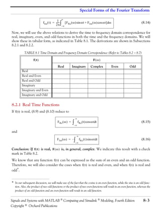


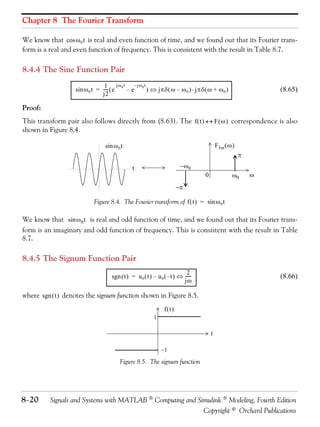


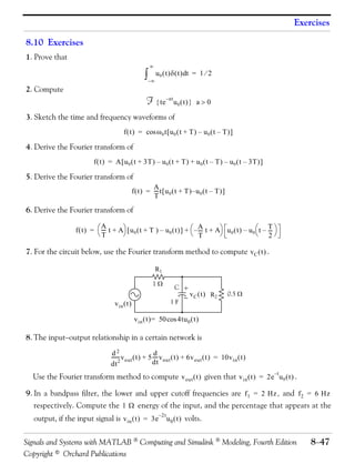


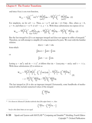


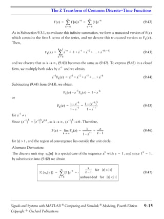


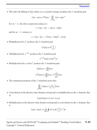


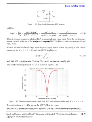


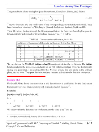


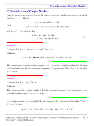


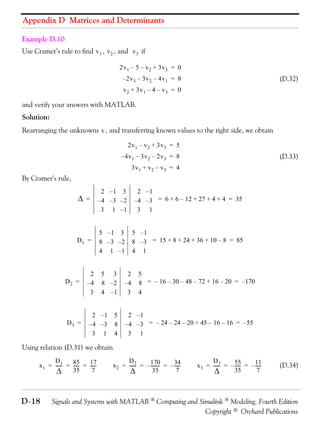


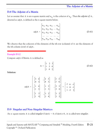


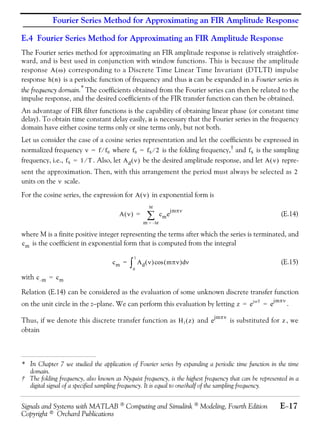


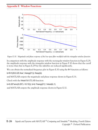


Signals and systems with matlab computing and simulink modeling
- 1. Signals and Systems with MATLAB ® Computing and Simulink ® Modeling Fourth Edition Steven T. Karris Includes step-by-step mn procedures N –1 – j2π -- -- -- - N X[ m ] = ∑ x [n ]e for designing n=0 analog and digital filters Orchard Publications www.orchardpublications.com
- 2. Signals and Systems with MATLAB Computing and Simulink Modeling Fourth Edition Steven T. Karris Orchard Publications www.orchardpublications.com
- 3. Signals and Systems with MATLAB® Computing and Simulink Modeling®, Fourth Edition Copyright © 2008 Orchard Publications. All rights reserved. Printed in the United States of America. No part of this publication may be reproduced or distributed in any form or by any means, or stored in a data base or retrieval system, without the prior written permission of the publisher. Direct all inquiries to Orchard Publications, [email protected] Product and corporate names are trademarks or registered trademarks of the Microsoft™ Corporation and The MathWorks™ Inc. They are used only for identification and explanation, without intent to infringe. Library of Congress Cataloging-in-Publication Data Catalog record is available from the Library of Congress Library of Congress Control Number: 2008927083 ISBN−13: 978−1−934404−12−6 ISBN−10: 1−934404−12−8 Copyright TX 5−471−562
- 4. Preface This text contains a comprehensive discussion on continuous and discrete time signals and systems with many MATLAB® and several Simulink® examples. It is written for junior and senior electrical and computer engineering students, and for self−study by working professionals. The prerequisites are a basic course in differential and integral calculus, and basic electric circuit theory. This book can be used in a two−quarter, or one semester course. This author has taught the subject material for many years and was able to cover all material in 16 weeks, with 2½ lecture hours per week. To get the most out of this text, it is highly recommended that Appendix A is thoroughly reviewed. This appendix serves as an introduction to MATLAB, and is intended for those who are not familiar with it. The Student Edition of MATLAB is an inexpensive, and yet a very powerful software package; it can be found in many college bookstores, or can be obtained directly from The MathWorks™ Inc., 3 Apple Hill Drive, Natick, MA 01760−2098 Phone: 508 647−7000, Fax: 508 647−7001 http://www.mathworks.com e−mail: [email protected] The elementary signals are reviewed in Chapter 1, and several examples are given. The purpose of this chapter is to enable the reader to express any waveform in terms of the unit step function, and subsequently the derivation of the Laplace transform of it. Chapters 2 through 4 are devoted to Laplace transformation and circuit analysis using this transform. Chapter 5 is an introduction to state−space and contains many illustrative examples. Chapter 6 discusses the impulse response. Chapters 7 and 8 are devoted to Fourier series and transform respectively. Chapter 9 introduces discrete−time signals and the Z transform. Considerable time was spent on Chapter 10 to present the Discrete Fourier transform and FFT with the simplest possible explanations. Chapter 11 contains a thorough discussion to analog and digital filters analysis and design procedures. As mentioned above, Appendix A is an introduction to MATLAB. Appendix B is an introduction to Simulink, Appendix C contains a review of complex numbers, and Appendix D is an introduction to matrix theory. New to the Second Edition This is an extensive revision of the first edition. The most notable change is the inclusion of the solutions to all exercises at the end of each chapter. It is in response to many readers who expressed a desire to obtain the solutions in order to check their solutions to those of the author and thereby enhancing their knowledge. Another reason is that this text is written also for self−
- 5. study by practicing engineers who need a review before taking more advanced courses such as digital image processing. Another major change is the addition of a rather comprehensive summary at the end of each chapter. Hopefully, this will be a valuable aid to instructors for preparation of view foils for presenting the material to their class. New to the Third Edition The most notable change is the inclusion of Simulink modeling examples. The pages where they appear can be found in the Table of Contents section of this text. Another change is the improvement of the plots generated by the latest revisions of the MATLAB® Student Version, Release 14. The author wishes to express his gratitude to the staff of The MathWorks™, the developers of MATLAB and Simulink, especially to Ms. Courtney Esposito, for the encouragement and unlimited support they have provided me with during the production of this text. Our heartfelt thanks also to Ms. Sally Wright, P.E., of Renewable Energy Research Laboratory University of Massachusetts, Amherst, for bringing some errors on the previous editions to our attention. New to the Fourth Edition The most notable change is the inclusion of Appendix E on window functions. The plots were generated generated with the latest revisions of the MATLAB® R2008a edition. Also, two end- of- chapter exercises were added in Chapter 10 to illustrate the use of the fft and ifft MATLAB functions The author wishes to express his gratitude to the staff of The MathWorks™, the developers of MATLAB and Simulink, especially to The MathWorks™ Book Program Team, for the encouragement and unlimited support they have provided me with during the production of this and all other texts by this publisher. Orchard Publications www.orchardpublications.com [email protected] 2
- 6. Table of Contents 1 Elementary Signals 1−1 1.1 Signals Described in Math Form .............................................................................1−1 1.2 The Unit Step Function ..........................................................................................1−2 1.3 The Unit Ramp Function ......................................................................................1−10 1.4 The Delta Function ............................................................................................... 1−11 1.4.1 The Sampling Property of the Delta Function ............................................1−12 1.4.2 The Sifting Property of the Delta Function ................................................1−13 1.5 Higher Order Delta Functions...............................................................................1−14 1.6 Summary ................................................................................................................1−22 1.7 Exercises.................................................................................................................1−23 1.8 Solutions to End−of−Chapter Exercises ................................................................1−24 MATLAB Computing Pages 1−20, 1−21 Simulink Modeling Page 1−18 2 The Laplace Transformation 2−1 2.1 Definition of the Laplace Transformation...............................................................2−1 2.2 Properties and Theorems of the Laplace Transform ...............................................2−2 2.2.1 Linearity Property ........................................................................................2−3 2.2.2 Time Shifting Property .................................................................................2−3 2.2.3 Frequency Shifting Property ........................................................................2−4 2.2.4 Scaling Property ...........................................................................................2−4 2.2.5 Differentiation in Time Domain Property ...................................................2−4 2.2.6 Differentiation in Complex Frequency Domain Property ...........................2−6 2.2.7 Integration in Time Domain Property .........................................................2−6 2.2.8 Integration in Complex Frequency Domain Property .................................2−8 2.2.9 Time Periodicity Property ............................................................................2−8 2.2.10 Initial Value Theorem..................................................................................2−9 2.2.11 Final Value Theorem .................................................................................2−10 2.2.12 Convolution in Time Domain Property.....................................................2−11 2.2.13 Convolution in Complex Frequency Domain Property.............................2−12 2.3 The Laplace Transform of Common Functions of Time.......................................2−14 2.3.1 The Laplace Transform of the Unit Step Function u 0 ( t ) ..........................2−14 2.3.2 The Laplace Transform of the Ramp Function u 1 ( t ) ................................2−14 2.3.3 The Laplace Transform of t n u0 ( t ) ..............................................................2−15 Signals and Systems with MATLAB Computing and Simulink Modeling, Third Edition i Copyright © Orchard Publications
- 7. 2.3.4 The Laplace Transform of the Delta Function δ ( t ) ................................. 2−18 2.3.5 The Laplace Transform of the Delayed Delta Function δ ( t – a ) .............. 2−18 2.3.6 The Laplace Transform of e –at u 0 ( t ) .......................................................... 2−19 – at 2.3.7 The Laplace Transform of t n e u 0 ( t ) ....................................................... 2−19 2.3.8 The Laplace Transform of sin ω t u 0 t ......................................................... 2−20 2.3.9 The Laplace Transform of cos ω t u 0 t ......................................................... 2−20 2.3.10 The Laplace Transform of e –at sin ω t u 0 ( t ) ................................................. 2−21 2.3.11 The Laplace Transform of e –at cos ω t u 0 ( t ) ................................................. 2−22 2.4 The Laplace Transform of Common Waveforms .................................................. 2−23 2.4.1 The Laplace Transform of a Pulse............................................................... 2−23 2.4.2 The Laplace Transform of a Linear Segment .............................................. 2−23 2.4.3 The Laplace Transform of a Triangular Waveform .................................... 2−24 2.4.4 The Laplace Transform of a Rectangular Periodic Waveform.................... 2−25 2.4.5 The Laplace Transform of a Half−Rectified Sine Waveform ..................... 2−26 2.5 Using MATLAB for Finding the Laplace Transforms of Time Functions ............ 2−27 2.6 Summary ................................................................................................................ 2−28 2.7 Exercises................................................................................................................. 2−31 The Laplace Transform of a Sawtooth Periodic Waveform ............................... 2−32 The Laplace Transform of a Full−Rectified Sine Waveform.............................. 2−32 2.8 Solutions to End−of−Chapter Exercises................................................................. 2−33 3 The Inverse Laplace Transform 3−1 3.1 The Inverse Laplace Transform Integral ..................................................................3−1 3.2 Partial Fraction Expansion........................................................................................3−1 3.2.1 Distinct Poles..................................................................................................3−2 3.2.2 Complex Poles ................................................................................................3−5 3.2.3 Multiple (Repeated) Poles..............................................................................3−8 3.3 Case where F(s) is Improper Rational Function.....................................................3−13 3.4 Alternate Method of Partial Fraction Expansion...................................................3−15 3.5 Summary .................................................................................................................3−19 3.6 Exercises..................................................................................................................3−21 3.7 Solutions to End−of−Chapter Exercises .................................................................3−22 MATLAB Computing Pages 3−3, 3−4, 3−5, 3−6, 3−8, 3−10, 3−12, 3−13, 3−14, 3−22 4 Circuit Analysis with Laplace Transforms 4−1 4.1 Circuit Transformation from Time to Complex Frequency.................................... 4−1 4.1.1 Resistive Network Transformation ............................................................... 4−1 4.1.2 Inductive Network Transformation .............................................................. 4−1 4.1.3 Capacitive Network Transformation ............................................................ 4−1 ii Signals and Systems with MATLAB Computing and Simulink Modeling, Third Edition Copyright © Orchard Publications
- 8. 4.2 Complex Impedance Z(s).........................................................................................4−8 4.3 Complex Admittance Y(s) .....................................................................................4−11 4.4 Transfer Functions .................................................................................................4−13 4.5 Using the Simulink Transfer Fcn Block.................................................................4−17 4.6 Summary.................................................................................................................4−20 4.7 Exercises .................................................................................................................4−21 4.8 Solutions to End−of−Chapter Exercises.................................................................4−24 MATLAB Computing Pages 4−6, 4−8, 4−12, 4−16, 4−17, 4−18, 4−26, 4−27, 4−28, 4−29, 4−34 Simulink Modeling Page 4−17 5 State Variables and State Equations 5−1 5.1 Expressing Differential Equations in State Equation Form................................... 5−1 5.2 Solution of Single State Equations ........................................................................ 5−6 5.3 The State Transition Matrix ................................................................................. 5−9 5.4 Computation of the State Transition Matrix ...................................................... 5−11 5.4.1 Distinct Eigenvalues ................................................................................. 5−11 5.4.2 Multiple (Repeated) Eigenvalues ............................................................. 5−15 5.5 Eigenvectors......................................................................................................... 5−18 5.6 Circuit Analysis with State Variables.................................................................. 5−22 5.7 Relationship between State Equations and Laplace Transform.......................... 5−30 5.8 Summary .............................................................................................................. 5−38 5.9 Exercises .............................................................................................................. 5−41 5.10 Solutions to End−of−Chapter Exercises .............................................................. 5−43 MATLAB Computing Pages 5−14, 5−15, 5−18, 5−26, 5−36, 5−48, 5−51 Simulink Modeling Pages 5−27, 5−37, 5−45 6 The Impulse Response and Convolution 6−1 6.1 The Impulse Response in Time Domain ................................................................ 6−1 6.2 Even and Odd Functions of Time .......................................................................... 6−4 6.3 Convolution ............................................................................................................ 6−7 6.4 Graphical Evaluation of the Convolution Integral................................................. 6−8 6.5 Circuit Analysis with the Convolution Integral ................................................... 6−18 6.6 Summary ............................................................................................................... 6−21 6.7 Exercises................................................................................................................ 6−23 Signals and Systems with MATLAB Computing and Simulink Modeling, Third Edition iii Copyright © Orchard Publications
- 9. 6.8 Solutions to End−of−Chapter Exercises................................................................ 6−25 MATLAB Applications Pages 6−12, 6−15, 6−30 7 Fourier Series 7−1 7.1 Wave Analysis......................................................................................................... 7−1 7.2 Evaluation of the Coefficients................................................................................. 7−2 7.3 Symmetry in Trigonometric Fourier Series ............................................................. 7−6 7.3.1 Symmetry in Square Waveform..................................................................... 7−8 7.3.2 Symmetry in Square Waveform with Ordinate Axis Shifted ........................ 7−8 7.3.3 Symmetry in Sawtooth Waveform................................................................. 7−9 7.3.4 Symmetry in Triangular Waveform ............................................................... 7−9 7.3.5 Symmetry in Fundamental, Second, and Third Harmonics........................ 7−10 7.4 Trigonometric Form of Fourier Series for Common Waveforms.......................... 7−10 7.4.1 Trigonometric Fourier Series for Square Waveform ................................... 7−11 7.4.2 Trigonometric Fourier Series for Sawtooth Waveform............................... 7−14 7.4.3 Trigonometric Fourier Series for Triangular Waveform ............................. 7−16 7.4.4 Trigonometric Fourier Series for Half−Wave Rectifier Waveform............. 7−17 7.4.5 Trigonometric Fourier Series for Full−Wave Rectifier Waveform.............. 7−20 7.5 Gibbs Phenomenon ............................................................................................... 7−24 7.6 Alternate Forms of the Trigonometric Fourier Series .......................................... 7−24 7.7 Circuit Analysis with Trigonometric Fourier Series............................................. 7−28 7.8 The Exponential Form of the Fourier Series........................................................ 7−31 7.9 Symmetry in Exponential Fourier Series .............................................................. 7−33 7.9.1 Even Functions ........................................................................................... 7−33 7.9.2 Odd Functions ............................................................................................ 7−34 7.9.3 Half-Wave Symmetry ................................................................................. 7−34 7.9.4 No Symmetry .............................................................................................. 7−34 7.9.5 Relation of C –n to C n ................................................................................ 7−34 7.10 Line Spectra.......................................................................................................... 7−36 7.11 Computation of RMS Values from Fourier Series................................................ 7−41 7.12 Computation of Average Power from Fourier Series ........................................... 7−44 7.13 Evaluation of Fourier Coefficients Using Excel® ................................................ 7−46 7.14 Evaluation of Fourier Coefficients Using MATLAB® ........................................ 7−47 7.15 Summary ............................................................................................................... 7−50 7.16 Exercises ............................................................................................................... 7−53 7.17 Solutions to End−of−Chapter Exercises ............................................................... 7−55 MATLAB Computing Pages 7−38, 7−47 iv Signals and Systems with MATLAB Computing and Simulink Modeling, Third Edition Copyright © Orchard Publications
- 10. Simulink Modeling Page 7−31 8 The Fourier Transform 8−1 8.1 Definition and Special Forms ................................................................................ 8−1 8.2 Special Forms of the Fourier Transform ................................................................ 8−2 8.2.1 Real Time Functions.................................................................................. 8−3 8.2.2 Imaginary Time Functions ......................................................................... 8−6 8.3 Properties and Theorems of the Fourier Transform .............................................. 8−9 8.3.1 Linearity...................................................................................................... 8−9 8.3.2 Symmetry.................................................................................................... 8−9 8.3.3 Time Scaling............................................................................................. 8−10 8.3.4 Time Shifting............................................................................................ 8−11 8.3.5 Frequency Shifting ................................................................................... 8−11 8.3.6 Time Differentiation ................................................................................ 8−12 8.3.7 Frequency Differentiation ........................................................................ 8−13 8.3.8 Time Integration ...................................................................................... 8−13 8.3.9 Conjugate Time and Frequency Functions.............................................. 8−13 8.3.10 Time Convolution .................................................................................... 8−14 8.3.11 Frequency Convolution............................................................................ 8−15 8.3.12 Area Under f ( t ) ........................................................................................ 8−15 8.3.13 Area Under F ( ω ) ...................................................................................... 8−15 8.3.14 Parseval’s Theorem................................................................................... 8−16 8.4 Fourier Transform Pairs of Common Functions.................................................. 8−18 8.4.1 The Delta Function Pair .......................................................................... 8−18 8.4.2 The Constant Function Pair .................................................................... 8−18 8.4.3 The Cosine Function Pair ........................................................................ 8−19 8.4.4 The Sine Function Pair............................................................................. 8−20 8.4.5 The Signum Function Pair........................................................................ 8−20 8.4.6 The Unit Step Function Pair .................................................................... 8−22 – jω 0 t 8.4.7 The e u0 ( t ) Function Pair .................................................................... 8−24 8.4.8 The ( cos ω 0 t ) ( u 0 t ) Function Pair ............................................................... 8−24 8.4.9 The ( sin ω 0 t ) ( u 0 t ) Function Pair ............................................................... 8−25 8.5 Derivation of the Fourier Transform from the Laplace Transform .................... 8−25 8.6 Fourier Transforms of Common Waveforms ...................................................... 8−27 8.6.1 The Transform of f ( t ) = A [ u 0 ( t + T ) – u 0 ( t – T ) ] ....................................... 8−27 8.6.2 The Transform of f ( t ) = A [ u 0 ( t ) – u 0 ( t – 2T ) ] ........................................... 8−28 8.6.3 The Transform of f ( t ) = A [ u 0 ( t + T ) + u 0 ( t ) – u 0 ( t – T ) – u 0 ( t – 2T ) ] ........... 8−29 Signals and Systems with MATLAB Computing and Simulink Modeling, Third Edition v Copyright © Orchard Publications
- 11. 8.6.4 The Transform of f ( t ) = A cos ω 0 t [ u0 ( t + T ) – u 0 ( t – T ) ] .............................. 8−30 8.6.5 The Transform of a Periodic Time Function with Period T..................... 8−31 ∞ 8.6.6 The Transform of the Periodic Time Function f ( t ) = A ∑ n = –∞ δ ( t – nT ) .... 8−32 8.7 Using MATLAB for Finding the Fourier Transform of Time Functions............ 8−33 8.8 The System Function and Applications to Circuit Analysis............................... 8−34 8.9 Summary .............................................................................................................. 8−42 8.10 Exercises............................................................................................................... 8−47 8.11 Solutions to End−of−Chapter Exercises .............................................................. 8−49 MATLAB Computing Pages 8−33, 8−34, 8−50, 8−54, 8−55, 8−56, 8−59, 8−60 9 Discrete−Time Systems and the Z Transform 9−1 9.1 Definition and Special Forms of the Z Transform ............................................... 9−1 9.2 Properties and Theorems of the Z Transform...................................................... 9−3 9.2.1 Linearity ..................................................................................................... 9−3 9.2.2 Shift of f [ n ]u 0 [ n ] in the Discrete−Time Domain ..................................... 9−3 9.2.3 Right Shift in the Discrete−Time Domain ................................................ 9−4 9.2.4 Left Shift in the Discrete−Time Domain................................................... 9−5 n 9.2.5 Multiplication by a in the Discrete−Time Domain................................. 9−6 – naT 9.2.6 Multiplication by e in the Discrete−Time Domain ........................... 9−6 9.2.7 Multiplication by n and n2 in the Discrete−Time Domain ..................... 9−6 9.2.8 Summation in the Discrete−Time Domain ............................................... 9−7 9.2.9 Convolution in the Discrete−Time Domain ............................................. 9−8 9.2.10 Convolution in the Discrete−Frequency Domain ..................................... 9−9 9.2.11 Initial Value Theorem ............................................................................... 9−9 9.2.12 Final Value Theorem............................................................................... 9−10 9.3 The Z Transform of Common Discrete−Time Functions.................................. 9−11 9.3.1 The Transform of the Geometric Sequence .............................................9−11 9.3.2 The Transform of the Discrete−Time Unit Step Function ......................9−14 9.3.3 The Transform of the Discrete−Time Exponential Sequence .................9−16 9.3.4 The Transform of the Discrete−Time Cosine and Sine Functions ..........9−16 9.3.5 The Transform of the Discrete−Time Unit Ramp Function....................9−18 9.4 Computation of the Z Transform with Contour Integration .............................9−20 9.5 Transformation Between s− and z−Domains .......................................................9−22 9.6 The Inverse Z Transform ...................................................................................9−25 vi Signals and Systems with MATLAB Computing and Simulink Modeling, Third Edition Copyright © Orchard Publications
- 12. 9.6.1 Partial Fraction Expansion ..................................................................... 9−25 9.6.2 The Inversion Integral............................................................................ 9−32 9.6.3 Long Division of Polynomials ................................................................ 9−36 9.7 The Transfer Function of Discrete−Time Systems ............................................ 9−38 9.8 State Equations for Discrete−Time Systems ...................................................... 9−45 9.9 Summary............................................................................................................. 9−48 9.10 Exercises ............................................................................................................. 9−53 9.11 Solutions to End−of−Chapter Exercises............................................................. 9−55 MATLAB Computing Pages 9−35, 9−37, 9−38, 9−41, 9−42, 9−59, 9−61 Simulink Modeling Page 9−44 Excel Plots Pages 9−35, 9−44 10 The DFT and the FFT Algorithm 10−1 10.1 The Discrete Fourier Transform (DFT) ............................................................10−1 10.2 Even and Odd Properties of the DFT ................................................................10−9 10.3 Common Properties and Theorems of the DFT ..............................................10−10 10.3.1 Linearity ...............................................................................................10−10 10.3.2 Time Shift ............................................................................................10−11 10.3.3 Frequency Shift....................................................................................10−12 10.3.4 Time Convolution ...............................................................................10−12 10.3.5 Frequency Convolution .......................................................................10−13 10.4 The Sampling Theorem ...................................................................................10−13 10.5 Number of Operations Required to Compute the DFT ..................................10−16 10.6 The Fast Fourier Transform (FFT) ..................................................................10−17 10.7 Summary...........................................................................................................10−28 10.8 Exercises ...........................................................................................................10−31 10.9 Solutions to End−of−Chapter Exercises...........................................................10−33 MATLAB Computing Pages 10−5, 10−7, 10−34 Excel Analysis ToolPak Pages 10−6, 10−8 11 Analog and Digital Filters 11.1 Filter Types and Classifications......................................................................... 11−1 11.2 Basic Analog Filters........................................................................................... 11−2 Signals and Systems with MATLAB Computing and Simulink Modeling, Third Edition vii Copyright © Orchard Publications
- 13. 11.2.1 RC Low−Pass Filter ............................................................................... 11−2 11.2.2 RC High−Pass Filter .............................................................................. 11−4 11.2.3 RLC Band−Pass Filter.............................................................................11−7 11.2.4 RLC Band−Elimination Filter ................................................................11−8 11.3 Low−Pass Analog Filter Prototypes ..................................................................11−10 11.3.1 Butterworth Analog Low−Pass Filter Design .......................................11−14 11.3.2 Chebyshev Type I Analog Low−Pass Filter Design..............................11−25 11.3.3 Chebyshev Type II Analog Low−Pass Filter Design ............................11−38 11.3.4 Elliptic Analog Low−Pass Filter Design ...............................................11−39 11.4 High−Pass, Band−Pass, and Band−Elimination Filter Design..........................11−41 11.5 Digital Filters ....................................................................................................11−51 11.6 Digital Filter Design with Simulink..................................................................11−70 11.6.1 The Direct Form I Realization of a Digital Filter.................................11−70 11.6.2 The Direct Form II Realization of a Digital Filter................................11−71 11.6.3 The Series Form Realization of a Digital Filter ....................................11−73 11.6.4 The Parallel Form Realization of a Digital Filter .................................11−75 11.6.5 The Digital Filter Design Block............................................................11−78 11.7 Summary ...........................................................................................................11−87 11.8 Exercises ...........................................................................................................11−91 11.9 Solutions to End−of−Chapter Exercises ...........................................................11−97 MATLAB Computing Pages 11−3, 11−4, 11−6, 11−7, 11−9, 11−15, 11−19, 11−23, 11−24, 11−31, 11−35, 11−36, 11−37, 11−38, 11−40, 11−41, 11−42, 11−43, 11−45, 11−46, 11−48, 11−50, 11−55, 11−56, 11−57, 11−60, 11−62, 11−64, 11−67, 11−68, and 11−97 through 11−106 Simulink Modeling Pages 11−71, 11−74, 11−77, 11−78, 11−80, 11−82, 11−83, 11−84 A Introduction to MATLAB A−1 A.1 MATLAB® and Simulink® ........................................................................... A−1 A.2 Command Window ......................................................................................... A−1 A.3 Roots of Polynomials ....................................................................................... A−3 A.4 Polynomial Construction from Known Roots ................................................. A−4 A.5 Evaluation of a Polynomial at Specified Values .............................................. A−6 A.6 Rational Polynomials ....................................................................................... A−8 A.7 Using MATLAB to Make Plots..................................................................... A−10 A.8 Subplots ......................................................................................................... A−18 A.9 Multiplication, Division, and Exponentiation .............................................. A−18 A.10 Script and Function Files .............................................................................. A−26 A.11 Display Formats ............................................................................................. A−31 viii Signals and Systems with MATLAB Computing and Simulink Modeling, Third Edition Copyright © Orchard Publications
- 14. MATLAB Computing Pages A−3 through A−8, A−10, A−13, A−14, A−16, A−17, A−21, A−22, A−24, A−27 B Introduction to Simulink B−1 B.1 Simulink and its Relation to MATLAB............................................................. B−1 B.2 Simulink Demos ............................................................................................... B−20 MATLAB Computing Page B−4 Simulink Modeling Pages B−7, B−12, B−14, B−18 C A Review of Complex Numbers C−1 C.1 Definition of a Complex Number....................................................................... C−1 C.2 Addition and Subtraction of Complex Numbers ............................................... C−2 C.3 Multiplication of Complex Numbers.................................................................. C−3 C.4 Division of Complex Numbers ........................................................................... C−4 C.5 Exponential and Polar Forms of Complex Numbers.......................................... C−4 MATLAB Computing Pages C−6, C−7, C−8 Simulink Modeling Page C−7 D Matrices and Determinants D−1 D.1 Matrix Definition.............................................................................................D−1 D.2 Matrix Operations ...........................................................................................D−2 D.3 Special Forms of Matrices................................................................................D−6 D.4 Determinants .................................................................................................D−10 D.5 Minors and Cofactors ....................................................................................D−12 D.6 Cramer’s Rule ................................................................................................D−17 D.7 Gaussian Elimination Method.......................................................................D−19 D.8 The Adjoint of a Matrix ................................................................................D−21 D.9 Singular and Non−Singular Matrices ............................................................D−21 D.10 The Inverse of a Matrix .................................................................................D−22 D.11 Solution of Simultaneous Equations with Matrices ......................................D−24 D.12 Exercises.........................................................................................................D−31 Signals and Systems with MATLAB Computing and Simulink Modeling, Third Edition ix Copyright © Orchard Publications
- 15. MATLAB Computing Pages D−3, D−4, D−5, D−7, D−8, D−9, D−10, D−12, D−19, D−23, D−27, D−29 Simulink Modeling Page D−3 Excel Spreadsheet Page D−28 E Window Functions E−1 E.1 Window Function Defined .................................................................................. E−1 E.2 Common Window Functions ............................................................................... E−1 E.2.1 Rectangular Window Function ................................................................. E−2 E.2.2 Triangular Window Function.................................................................... E−5 E.2.3 Hanning Window Function....................................................................... E−7 E.2.4 Hamming Window Function..................................................................... E−9 E.2.5 Blackman Window Function................................................................... E−12 E.2.6 Kaiser Family of Window Functions ....................................................... E−14 E.3 Other Window Functions .................................................................................. E−15 E.4 Fourier Series Method for Approximating an FIR Amplitude Response .......... E−17 References R−1 Index IN−1 x Signals and Systems with MATLAB Computing and Simulink Modeling, Third Edition Copyright © Orchard Publications
- 16. Chapter 1 Elementary Signals T his chapter begins with a discussion of elementary signals that may be applied to electric networks. The unit step, unit ramp, and delta functions are then introduced. The sampling and sifting properties of the delta function are defined and derived. Several examples for expressing a variety of waveforms in terms of these elementary signals are provided. Throughout this text, a left justified horizontal bar will denote the beginning of an example, and a right justi- fied horizontal bar will denote the end of the example. These bars will not be shown whenever an example begins at the top of a page or at the bottom of a page. Also, when one example follows immediately after a previous example, the right justified bar will be omitted. 1.1 Signals Described in Math Form Consider the network of Figure 1.1 where the switch is closed at time t = 0 . R t = 0 + + v out open terminals − vS − Figure 1.1. A switched network with open terminals We wish to describe v out in a math form for the time interval – ∞ < t < +∞ . To do this, it is conve- nient to divide the time interval into two parts, – ∞ < t < 0 , and 0 < t < ∞ . For the time interval – ∞ < t < 0 , the switch is open and therefore, the output voltage v out is zero. In other words, v out = 0 for – ∞ < t < 0 (1.1) For the time interval 0 < t < ∞ , the switch is closed. Then, the input voltage v S appears at the output, i.e., v out = v S for 0 < t < ∞ (1.2) Combining (1.1) and (1.2) into a single relationship, we obtain 0 –∞ < t < 0 v out = (1.3) vS 0 < t < ∞ Signals and Systems with MATLAB Computing and Simulink Modeling, Fourth Edition 1−1 Copyright © Orchard Publications
- 17. Chapter 1 Elementary Signals We can express (1.3) by the waveform shown in Figure 1.2. v out vS 0 t Figure 1.2. Waveform for v out as defined in relation (1.3) The waveform of Figure 1.2 is an example of a discontinuous function. A function is said to be dis- continuous if it exhibits points of discontinuity, that is, the function jumps from one value to another without taking on any intermediate values. 1.2 The Unit Step Function u 0 ( t ) A well known discontinuous function is the unit step function u 0 ( t ) * which is defined as 0 t<0 u0 ( t ) = (1.4) 1 t>0 It is also represented by the waveform of Figure 1.3. u0 ( t ) 1 0 t Figure 1.3. Waveform for u 0 ( t ) In the waveform of Figure 1.3, the unit step function u 0 ( t ) changes abruptly from 0 to 1 at t = 0 . But if it changes at t = t 0 instead, it is denoted as u 0 ( t – t 0 ) . In this case, its waveform and definition are as shown in Figure 1.4 and relation (1.5) respectively. 1 u0 ( t – t0 ) t 0 t0 Figure 1.4. Waveform for u 0 ( t – t 0 ) * In some books, the unit step function is denoted as u ( t ) , that is, without the subscript 0. In this text, however, we will reserve the u ( t ) designation for any input when we will discuss state variables in Chapter 5. 1−2 Signals and Systems with MATLAB Computing and Simulink Modeling, Fourth Edition Copyright © Orchard Publications
- 18. The Unit Step Function 0 t < t0 u0 ( t – t0 ) = (1.5) 1 t > t0 If the unit step function changes abruptly from 0 to 1 at t = – t 0 , it is denoted as u 0 ( t + t 0 ) . In this case, its waveform and definition are as shown in Figure 1.5 and relation (1.6) respectively. u0 ( t + t0 ) 1 −t0 0 t Figure 1.5. Waveform for u 0 ( t + t 0 ) 0 t < –t0 u0 ( t + t0 ) = (1.6) 1 t > –t0 Example 1.1 Consider the network of Figure 1.6, where the switch is closed at time t = T . R t = T + + v out open terminals − vS − Figure 1.6. Network for Example 1.1 Express the output voltage v out as a function of the unit step function, and sketch the appropriate waveform. Solution: For this example, the output voltage v out = 0 for t < T , and v out = v S for t > T . Therefore, v out = v S u 0 ( t – T ) (1.7) and the waveform is shown in Figure 1.7. Signals and Systems with MATLAB Computing and Simulink Modeling, Fourth Edition 1−3 Copyright © Orchard Publications
- 19. Chapter 1 Elementary Signals vS u0 ( t – T ) v out t 0 T Figure 1.7. Waveform for Example 1.1 Other forms of the unit step function are shown in Figure 1.8. Τ −Τ t t t 0 0 0 (a) (b) (c) −A −A −A –A u0 ( t ) –A u0 ( t – T ) –A u0 ( t + T ) Au 0 ( – t ) Au 0 ( – t + T ) Au 0 ( – t – T ) A A A t t −Τ 0 t 0 (d) 0 Τ (e) (f) Τ −Τ t t 0 t 0 (g) 0 (h) (i) −A −A −A –A u0 ( –t ) –A u0 ( – t + T ) –A u0 ( – t – T ) Figure 1.8. Other forms of the unit step function Unit step functions can be used to represent other time−varying functions such as the rectangular pulse shown in Figure 1.9. u0 ( t ) 1 1 t t t 0 1 0 0 (c) (a) (b) –u0 ( t – 1 ) Figure 1.9. A rectangular pulse expressed as the sum of two unit step functions 1−4 Signals and Systems with MATLAB Computing and Simulink Modeling, Fourth Edition Copyright © Orchard Publications
- 20. The Unit Step Function Thus, the pulse of Figure 1.9(a) is the sum of the unit step functions of Figures 1.9(b) and 1.9(c) and it is represented as u 0 ( t ) – u 0 ( t – 1 ) . The unit step function offers a convenient method of describing the sudden application of a volt- age or current source. For example, a constant voltage source of 24 V applied at t = 0 , can be denoted as 24u 0 ( t ) V . Likewise, a sinusoidal voltage source v ( t ) = V m cos ωt V that is applied to a circuit at t = t0 , can be described as v ( t ) = ( V m cos ωt )u 0 ( t – t 0 ) V . Also, if the excitation in a circuit is a rectangular, or triangular, or sawtooth, or any other recurring pulse, it can be repre- sented as a sum (difference) of unit step functions. Example 1.2 Express the square waveform of Figure 1.10 as a sum of unit step functions. The vertical dotted lines indicate the discontinuities at T, 2T, 3T , and so on. v(t) A T 2T 3T t 0 –A Figure 1.10. Square waveform for Example 1.2 Solution: Line segment has height A , starts at t = 0 , and terminates at t = T . Then, as in Example 1.1, this segment is expressed as v1 ( t ) = A [ u0 ( t ) – u0 ( t – T ) ] (1.8) Line segment has height – A , starts at t = T and terminates at t = 2T . This segment is expressed as v 2 ( t ) = – A [ u 0 ( t – T ) – u 0 ( t – 2T ) ] (1.9) Line segment has height A , starts at t = 2T and terminates at t = 3T . This segment is expressed as v 3 ( t ) = A [ u 0 ( t – 2T ) – u 0 ( t – 3T ) ] (1.10) Line segment has height – A , starts at t = 3T , and terminates at t = 4T . It is expressed as v 4 ( t ) = – A [ u 0 ( t – 3T ) – u 0 ( t – 4T ) ] (1.11) Signals and Systems with MATLAB Computing and Simulink Modeling, Fourth Edition 1−5 Copyright © Orchard Publications
- 21. Chapter 1 Elementary Signals Thus, the square waveform of Figure 1.10 can be expressed as the summation of (1.8) through (1.11), that is, v ( t ) = v1 ( t ) + v2 ( t ) + v3 ( t ) + v4 ( t ) = A [ u 0 ( t ) – u 0 ( t – T ) ] – A [ u 0 ( t – T ) – u 0 ( t – 2T ) ] (1.12) +A [ u 0 ( t – 2T ) – u 0 ( t – 3T ) ] – A [ u 0 ( t – 3T ) – u 0 ( t – 4T ) ] Combining like terms, we obtain v ( t ) = A [ u 0 ( t ) – 2u 0 ( t – T ) + 2u 0 ( t – 2T ) – 2u 0 ( t – 3T ) + … ] (1.13) Example 1.3 Express the symmetric rectangular pulse of Figure 1.11 as a sum of unit step functions. i(t) A t –T ⁄ 2 0 T⁄2 Figure 1.11. Symmetric rectangular pulse for Example 1.3 Solution: This pulse has height A , starts at t = – T ⁄ 2 , and terminates at t = T ⁄ 2 . Therefore, with refer- ence to Figures 1.5 and 1.8 (b), we obtain i ( t ) = Au 0 t + -- – Au 0 t – -- = A u 0 t + -- – u 0 t – -- T T T T - 2 - - 2 - (1.14) 2 2 Example 1.4 Express the symmetric triangular waveform of Figure 1.12 as a sum of unit step functions. v(t) 1 t –T ⁄ 2 0 T⁄2 Figure 1.12. Symmetric triangular waveform for Example 1.4 Solution: 1−6 Signals and Systems with MATLAB Computing and Simulink Modeling, Fourth Edition Copyright © Orchard Publications
- 22. The Unit Step Function We first derive the equations for the linear segments and shown in Figure 1.13. 2 v( t) 2 -- t + 1 - 1 – -- t + 1 - T T t –T ⁄ 2 0 T⁄2 Figure 1.13. Equations for the linear segments of Figure 1.12 For line segment , v 1 ( t ) = -- t + 1 u 0 t + -- – u 0 ( t ) 2 T T - 2 - (1.15) and for line segment , v 2 ( t ) = – -- t + 1 u 0 ( t ) – u 0 t – T 2- -- - (1.16) T 2 Combining (1.15) and (1.16), we obtain v ( t ) = v1 ( t ) + v2 ( t ) (1.17) = -- t + 1 u 0 t + T – u 0 ( t ) + – -- t + 1 u 0 ( t ) – u 0 t – T 2- 2 -- - - -- - T 2 T 2 Example 1.5 Express the waveform of Figure 1.14 as a sum of unit step functions. v( t) 3 2 1 t 0 1 2 3 Figure 1.14. Waveform for Example 1.5 Solution: Signals and Systems with MATLAB Computing and Simulink Modeling, Fourth Edition 1−7 Copyright © Orchard Publications
- 23. Chapter 1 Elementary Signals As in the previous example, we first find the equations of the linear segments linear segments and shown in Figure 1.15. v(t) 3 2 2t + 1 1 –t+3 t 0 1 2 3 Figure 1.15. Equations for the linear segments of Figure 1.14 Following the same procedure as in the previous examples, we obtain v ( t ) = ( 2t + 1 ) [ u 0 ( t ) – u 0 ( t – 1 ) ] + 3 [ u 0 ( t – 1 ) – u 0 ( t – 2 ) ] + ( – t + 3 ) [ u0 ( t – 2 ) – u0 ( t – 3 ) ] Multiplying the values in parentheses by the values in the brackets, we obtain v ( t ) = ( 2t + 1 )u 0 ( t ) – ( 2t + 1 )u 0 ( t – 1 ) + 3u 0 ( t – 1 ) – 3u 0 ( t – 2 ) + ( – t + 3 )u 0 ( t – 2 ) – ( – t + 3 )u 0 ( t – 3 ) v ( t ) = ( 2t + 1 )u 0 ( t ) + [ – ( 2t + 1 ) + 3 ]u 0 ( t – 1 ) + [ – 3 + ( – t + 3 ) ]u 0 ( t – 2 ) – ( – t + 3 )u 0 ( t – 3 ) and combining terms inside the brackets, we obtain v ( t ) = ( 2t + 1 )u 0 ( t ) – 2 ( t – 1 )u 0 ( t – 1 ) – t u 0 ( t – 2 ) + ( t – 3 )u 0 ( t – 3 ) (1.18) Two other functions of interest are the unit ramp function, and the unit impulse or delta function. We will introduce them with the examples that follow. Example 1.6 In the network of Figure 1.16 i S is a constant current source and the switch is closed at time t = 0 . Express the capacitor voltage v C ( t ) as a function of the unit step. 1−8 Signals and Systems with MATLAB Computing and Simulink Modeling, Fourth Edition Copyright © Orchard Publications
- 24. The Unit Step Function R t = 0 + vC ( t ) − iS C Figure 1.16. Network for Example 1.6 Solution: The current through the capacitor is i C ( t ) = i S = cons tan t , and the capacitor voltage v C ( t ) is t 1 * v C ( t ) = --- C - ∫– ∞ i C ( τ ) dτ (1.19) where τ is a dummy variable. Since the switch closes at t = 0 , we can express the current i C ( t ) as iC ( t ) = iS u0 ( t ) (1.20) and assuming that v C ( t ) = 0 for t < 0 , we can write (1.19) as iS 0 1 t --- - ∫–∞ u0 ( τ ) dτ iS t v C ( t ) = --- C - ∫– ∞ i S u 0 ( τ ) dτ = C + --- C - ∫ 0 u 0 ( τ ) dτ (1.21) 0 or iS v C ( t ) = ---- tu 0 ( t ) - (1.22) C Therefore, we see that when a capacitor is charged with a constant current, the voltage across it is a linear function and forms a ramp with slope i S ⁄ C as shown in Figure 1.17. vC ( t ) slope = i S ⁄ C t 0 Figure 1.17. Voltage across a capacitor when charged with a constant current source * Since the initial condition for the capacitor voltage was not specified, we express this integral with –∞ at the lower limit of integration so that any non-zero value prior to t < 0 would be included in the integration. Signals and Systems with MATLAB Computing and Simulink Modeling, Fourth Edition 1−9 Copyright © Orchard Publications
- 25. Chapter 1 Elementary Signals 1.3 The Unit Ramp Function u 1 ( t ) The unit ramp function, denoted as u 1 ( t ) , is defined as t u1 ( t ) = ∫– ∞ u 0 ( τ ) d τ (1.23) where τ is a dummy variable. We can evaluate the integral of (1.23) by considering the area under the unit step function u 0 ( t ) from – ∞ to t as shown in Figure 1.18. Area = 1 × τ = τ = t 1 t τ Figure 1.18. Area under the unit step function from – ∞ to t Therefore, we define u 1 ( t ) as 0 t<0 u1 ( t ) = (1.24) t t≥0 Since u 1 ( t ) is the integral of u 0 ( t ) , then u 0 ( t ) must be the derivative of u 1 ( t ) , i.e., d ---- u 1 ( t ) = u 0 ( t ) - (1.25) dt Higher order functions of t can be generated by repeated integration of the unit step function. For example, integrating u 0 ( t ) twice and multiplying by 2 , we define u 2 ( t ) as 0 t<0 t u2 ( t ) = 2 t t≥0 or u2 ( t ) = 2 ∫–∞ u1 ( τ ) dτ (1.26) Similarly, 0 t<0 t u3 ( t ) = 3 t t≥0 or u3 ( t ) = 3 ∫–∞ u2 ( τ ) dτ (1.27) and in general, 0 t<0 t un ( t ) = n t t≥0 or un ( t ) = 3 ∫– ∞ u n – 1 ( τ ) d τ (1.28) Also, 1−10 Signals and Systems with MATLAB Computing and Simulink Modeling, Fourth Edition Copyright © Orchard Publications
- 26. The Delta Function 1d u n – 1 ( t ) = -- ---- u n ( t ) - - (1.29) n dt Example 1.7 In the network of Figure 1.19, the switch is closed at time t = 0 and i L ( t ) = 0 for t < 0 . Express the inductor current i L ( t ) in terms of the unit step function. R t = 0 + iL ( t ) vL ( t ) iS L − Figure 1.19. Network for Example 1.7 Solution: The voltage across the inductor is di L v L ( t ) = L ------- (1.30) dt and since the switch closes at t = 0 , iL ( t ) = iS u0 ( t ) (1.31) Therefore, we can write (1.30) as d v L ( t ) = Li S ---- u 0 ( t ) - (1.32) dt But, as we know, u 0 ( t ) is constant ( 0 or 1 ) for all time except at t = 0 where it is discontinuous. Since the derivative of any constant is zero, the derivative of the unit step u 0 ( t ) has a non−zero value only at t = 0 . The derivative of the unit step function is defined in the next section. 1.4 The Delta Function δ ( t ) The unit impulse or delta function, denoted as δ ( t ) , is the derivative of the unit step u 0 ( t ) . It is also defined as t ∫– ∞ δ ( τ ) d τ = u0 ( t ) (1.33) and δ ( t ) = 0 for all t ≠ 0 (1.34) Signals and Systems with MATLAB Computing and Simulink Modeling, Fourth Edition 1−11 Copyright © Orchard Publications
- 27. Chapter 1 Elementary Signals To better understand the delta function δ ( t ) , let us represent the unit step u 0 ( t ) as shown in Fig- ure 1.20 (a). 1 Figure (a) 0 −ε ε t 1 Area =1 2ε Figure (b) 0 −ε ε t Figure 1.20. Representation of the unit step as a limit The function of Figure 1.20 (a) becomes the unit step as ε → 0 . Figure 1.20 (b) is the derivative of Figure 1.20 (a), where we see that as ε → 0 , 1 ⁄ 2 ε becomes unbounded, but the area of the rect- angle remains 1 . Therefore, in the limit, we can think of δ ( t ) as approaching a very large spike or impulse at the origin, with unbounded amplitude, zero width, and area equal to 1 . Two useful properties of the delta function are the sampling property and the sifting property. 1.4.1 The Sampling Property of the Delta Function δ ( t ) The sampling property of the delta function states that f ( t )δ ( t – a ) = f ( a )δ ( t ) (1.35) or, when a = 0 , f ( t )δ ( t ) = f ( 0 )δ ( t ) (1.36) that is, multiplication of any function f ( t ) by the delta function δ ( t ) results in sampling the func- tion at the time instants where the delta function is not zero. The study of discrete−time systems is based on this property. Proof: Since δ ( t ) = 0 for t < 0 and t > 0 then, f ( t )δ ( t ) = 0 for t < 0 and t > 0 (1.37) We rewrite f ( t ) as f(t) = f(0) + [f(t) – f(0)] (1.38) Integrating (1.37) over the interval – ∞ to t and using (1.38), we obtain 1−12 Signals and Systems with MATLAB Computing and Simulink Modeling, Fourth Edition Copyright © Orchard Publications
- 28. The Delta Function t t t ∫– ∞ f ( τ )δ ( τ ) dτ = ∫– ∞ f ( 0 )δ ( τ ) dτ + ∫–∞ [ f ( τ ) – f ( 0 ) ]δ ( τ ) dτ (1.39) The first integral on the right side of (1.39) contains the constant term f ( 0 ) ; this can be written outside the integral, that is, t t ∫– ∞ f ( 0 )δ ( τ ) dτ = f ( 0 ) ∫– ∞ δ ( τ ) d τ (1.40) The second integral of the right side of (1.39) is always zero because δ ( t ) = 0 for t < 0 and t > 0 and [f(τ ) – f(0 ) ] τ=0 = f(0 ) – f( 0) = 0 Therefore, (1.39) reduces to t t ∫– ∞ f ( τ )δ ( τ ) dτ = f ( 0 ) ∫– ∞ δ ( τ ) d τ (1.41) Differentiating both sides of (1.41), and replacing τ with t , we obtain f ( t )δ ( t ) = f ( 0 )δ ( t ) (1.42) Sampling Property of δ ( t ) 1.4.2 The Sifting Property of the Delta Function δ ( t ) The sifting property of the delta function states that ∞ ∫–∞ f ( t )δ ( t – α ) dt = f(α) (1.43) that is, if we multiply any function f ( t ) by δ ( t – α ) , and integrate from – ∞ to +∞ , we will obtain the value of f ( t ) evaluated at t = α . Proof: Let us consider the integral b ∫a f ( t )δ ( t – α ) dt where a < α < b (1.44) We will use integration by parts to evaluate this integral. We recall from the derivative of prod- ucts that d ( xy ) = xdy + ydx or xdy = d ( xy ) – ydx (1.45) and integrating both sides we obtain Signals and Systems with MATLAB Computing and Simulink Modeling, Fourth Edition 1−13 Copyright © Orchard Publications
- 29. Chapter 1 Elementary Signals ∫ x dy = xy – y dx ∫ (1.46) Now, we let x = f ( t ) ; then, dx = f ′( t ) . We also let dy = δ ( t – α ) ; then, y = u 0 ( t – α ) . By sub- stitution into (1.44), we obtain b b ∫a ∫a u0 ( t – α )f ′( t ) dt b f ( t )δ ( t – α ) dt = f ( t )u 0 ( t – α ) – (1.47) a We have assumed that a < α < b ; therefore, u 0 ( t – α ) = 0 for α < a , and thus the first term of the right side of (1.47) reduces to f ( b ) . Also, the integral on the right side is zero for α < a , and there- fore, we can replace the lower limit of integration a by α . We can now rewrite (1.47) as b b ∫a f ( t )δ ( t – α ) dt = f ( b ) – ∫α f ′ ( t ) d t = f( b) – f( b) + f(α ) and letting a → – ∞ and b → ∞ for any α < ∞ , we obtain ∞ ∫–∞ f ( t )δ ( t – α ) dt = f ( α ) (1.48) Sifting Property of δ ( t ) 1.5 Higher Order Delta Functions An nth-order delta function is defined as the nth derivative of u 0 ( t ) , that is, n n δ δ ( t ) = ---- [ u 0 ( t ) ] - (1.49) dt The function δ' ( t ) is called doublet, δ'' ( t ) is called triplet, and so on. By a procedure similar to the derivation of the sampling property of the delta function, we can show that f ( t )δ' ( t – a ) = f ( a )δ' ( t – a ) – f ' ( a )δ ( t – a ) (1.50) Also, the derivation of the sifting property of the delta function can be extended to show that ∞ n nd ∫ n f ( t )δ ( t – α ) dt = ( – 1 ) ------- [ f ( t ) ] - n (1.51) –∞ dt t=α 1−14 Signals and Systems with MATLAB Computing and Simulink Modeling, Fourth Edition Copyright © Orchard Publications
- 30. Higher Order Delta Functions Example 1.8 Evaluate the following expressions: ∞ a. 3t δ ( t – 1 ) b. ∫–∞ tδ ( t – 2 ) dt c. t δ' ( t – 3 ) 4 2 Solution: a. The sampling property states that f ( t )δ ( t – a ) = f ( a )δ ( t – a ) For this example, f ( t ) = 3t and 4 a = 1 . Then, 4 4 3t δ ( t – 1 ) = { 3t t=1 }δ ( t – 1 ) = 3δ ( t – 1 ) ∞ b. The sifting property states that ∫–∞ f ( t )δ ( t – α ) dt = f ( α ) . For this example, f ( t ) = t and α = 2 . Then, ∞ ∫–∞ tδ ( t – 2 ) dt = f ( 2 ) = t t = 2 = 2 c. The given expression contains the doublet; therefore, we use the relation f ( t )δ' ( t – a ) = f ( a )δ' ( t – a ) – f ' ( a )δ ( t – a ) Then, for this example, 2 2 d- 2 t δ' ( t – 3 ) = t t=3 δ' ( t – 3 ) – ---- t t=3 δ ( t – 3 ) = 9δ' ( t – 3 ) – 6δ ( t – 3 ) dt Example 1.9 a. Express the voltage waveform v ( t ) shown in Figure 1.21 as a sum of unit step functions for the time interval – 1 < t < 7 s . b. Using the result of part (a), compute the derivative of v ( t ) and sketch its waveform. Signals and Systems with MATLAB Computing and Simulink Modeling, Fourth Edition 1−15 Copyright © Orchard Publications
- 31. Chapter 1 Elementary Signals v(t) (V) 3 2 1 −1 1 2 3 4 5 6 7 0 t (s) −1 −2 Figure 1.21. Waveform for Example 1.9 Solution: a. We begin with the derivation of the equations for the linear segments of the given waveform as shown in Figure 1.22. v(t) (V) v(t) –t+5 3 2 –t+6 1 −1 1 2 3 4 5 6 7 0 t (s) −1 2t −2 Figure 1.22. Equations for the linear segments of Figure 1.21 Next, we express v ( t ) in terms of the unit step function u 0 ( t ) , and we obtain v ( t ) = 2t [ u 0 ( t + 1 ) – u 0 ( t – 1 ) ] + 2 [ u 0 ( t – 1 ) – u 0 ( t – 2 ) ] + ( – t + 5 ) [ u0 ( t – 2 ) – u0 ( t – 4 ) ] + [ u0 ( t – 4 ) – u0 ( t – 5 ) ] (1.52) + ( – t + 6 ) [ u0 ( t – 5 ) – u0 ( t – 7 ) ] Multiplying and collecting like terms in (1.52), we obtain 1−16 Signals and Systems with MATLAB Computing and Simulink Modeling, Fourth Edition Copyright © Orchard Publications
- 32. Higher Order Delta Functions v ( t ) = 2tu 0 ( t + 1 ) – 2tu 0 ( t – 1 ) – 2u 0 ( t – 1 ) – 2u 0 ( t – 2 ) – tu 0 ( t – 2 ) + 5u 0 ( t – 2 ) + tu 0 ( t – 4 ) – 5u 0 ( t – 4 ) + u 0 ( t – 4 ) – u 0 ( t – 5 ) – tu 0 ( t – 5 ) + 6u 0 ( t – 5 ) + tu 0 ( t – 7 ) – 6u 0 ( t – 7 ) or v ( t ) = 2tu 0 ( t + 1 ) + ( – 2t + 2 )u 0 ( t – 1 ) + ( – t + 3 )u 0 ( t – 2 ) + ( t – 4 )u 0 ( t – 4 ) + ( – t + 5 )u 0 ( t – 5 ) + ( t – 6 )u 0 ( t – 7 ) b. The derivative of v ( t ) is dv = 2u ( t + 1 ) + 2tδ ( t + 1 ) – 2u ( t – 1 ) + ( – 2t + 2 )δ ( t – 1 ) ----- - 0 0 dt – u 0 ( t – 2 ) + ( – t + 3 )δ ( t – 2 ) + u 0 ( t – 4 ) + ( t – 4 )δ ( t – 4 ) (1.53) – u 0 ( t – 5 ) + ( – t + 5 )δ ( t – 5 ) + u 0 ( t – 7 ) + ( t – 6 )δ ( t – 7 ) From the given waveform, we observe that discontinuities occur only at t = – 1 , t = 2 , and t = 7 . Therefore, δ ( t – 1 ) = 0 , δ ( t – 4 ) = 0 , and δ ( t – 5 ) = 0 , and the terms that contain these delta functions vanish. Also, by application of the sampling property, 2tδ ( t + 1 ) = { 2t t = –1 }δ ( t + 1 ) = – 2δ ( t + 1 ) ( – t + 3 )δ ( t – 2 ) = { ( – t + 3 ) t=2 }δ ( t – 2 ) = δ ( t – 2 ) ( t – 6 )δ ( t – 7 ) = { ( t – 6 ) t=7 }δ ( t – 7 ) = δ ( t – 7 ) and by substitution into (1.53), we obtain dv = 2u ( t + 1 ) – 2 δ ( t + 1 ) – 2u ( t – 1 ) – u ( t – 2 ) ----- - 0 0 0 dt (1.54) + δ ( t – 2 ) + u0 ( t – 4 ) – u0 ( t – 5 ) + u0 ( t – 7 ) + δ ( t – 7 ) The plot of dv ⁄ dt is shown in Figure 1.23. Signals and Systems with MATLAB Computing and Simulink Modeling, Fourth Edition 1−17 Copyright © Orchard Publications
- 33. Chapter 1 Elementary Signals dv (V ⁄ s) ----- - dt 2 δ(t – 2) δ(t – 7) 1 −1 0 1 2 3 4 5 6 7 t (s) −1 – 2δ ( t + 1 ) Figure 1.23. Plot of the derivative of the waveform of Figure 1.21 We observe that a negative spike of magnitude 2 occurs at t = – 1 , and two positive spikes of magnitude 1 occur at t = 2 , and t = 7 . These spikes occur because of the discontinuities at these points. It would be interesting to observe the given signal and its derivative on the Scope block of the Simulink* model of Figure 1.24. They are shown in Figure 1.25. Figure 1.24. Simulink model for Example 1.9 The waveform created by the Signal Builder block is shown in Figure 1.25. * A brief introduction to Simulink is presented in Appendix B. For a detailed procedure for generating piece-wise linear functions with Simulink’s Signal Builder block, please refer to Introduction to Simulink with Engineering Applications, ISBN 0−9744239−7−1 1−18 Signals and Systems with MATLAB Computing and Simulink Modeling, Fourth Edition Copyright © Orchard Publications
- 34. Higher Order Delta Functions Figure 1.25. Piece−wise linear waveform for the Signal Builder block in Figure 1.24 The waveform in Figure 1.25 is created with the following procedure: 1. We open a new model by clicking on the new model icon shown as a blank page on the left cor- ner of the top menu bar. Initially, the name Untitled appears on the top of this new model. We save it with the name Figure_1.25 and Simulink appends the .mdl extension to it. 2. From the Sources library, we drag the Signal Builder block into this new model. We also drag the Derivative block from the Continuous library, the Bus Creator block from the Com- monly Used Blocks library, and the Scope block into this model, and we interconnect these blocks as shown in Figure 1.24. 3. We double−click on the Signal Builder block in Figure 1.24, and on the plot which appears as a square pulse, we click on the y−axis and we enter Minimum: −2.5, and Maximum: 3.5. Like- wise we right−click anywhere on the plot and we specify the Change Time Range at Min time: −2, and Max time: 8. 4. To select a particular point, we position the mouse cursor over that point and we left−click. A circle is drawn around that point to indicate that it is selected. 5. To select a line segment, we left−click on that segment. That line segment is now shown as a thick line indicating that it is selected. To deselect it, we press the Esc key. Signals and Systems with MATLAB Computing and Simulink Modeling, Fourth Edition 1−19 Copyright © Orchard Publications
- 35. Chapter 1 Elementary Signals 6. To drag a line segment to a new position, we place the mouse cursor over that line segment and the cursor shape shows the position in which we can drag the segment. 7. To drag a point along the y−axis, we move the mouse cursor over that point, and the cursor changes to a circle indicating that we can drag that point. Then, we can move that point in a direction parallel to the x−axis. 8. To drag a point along the x−axis, we select that point, and we hold down the Shift key while dragging that point. 9. When we select a line segment on the time axis (x−axis) we observe that at the lower end of the waveform display window the Left Point and Right Point fields become visible. We can then reshape the given waveform by specifying the Time (T) and Amplitude (Y) points. Figure 1.26. Waveforms for the Simulink model of Figure 1.24 The two positive spikes that occur at t = 2 , and t = 7 , are clearly shown in Figure 1.26. MATLAB* has built-in functions for the unit step, and the delta functions. These are denoted by the names of the mathematicians who used them in their work. The unit step function u 0 ( t ) is referred to as Heaviside(t), and the delta function δ ( t ) is referred to as Dirac(t). Their use is illus- trated with the examples below. syms k a t; % Define symbolic variables u=k*sym('Heaviside(t−a)') % Create unit step function at t = a u = k*Heaviside(t-a) d=diff(u) % Compute the derivative of the unit step function d = k*Dirac(t-a) * An introduction to MATLAB® is given in Appendix A. 1−20 Signals and Systems with MATLAB Computing and Simulink Modeling, Fourth Edition Copyright © Orchard Publications
- 36. Higher Order Delta Functions int(d) % Integrate the delta function ans = Heaviside(t-a)*k Signals and Systems with MATLAB Computing and Simulink Modeling, Fourth Edition 1−21 Copyright © Orchard Publications
- 37. Chapter 1 Elementary Signals 1.6 Summary • The unit step function u 0 ( t ) is defined as 0 t<0 u0 ( t ) = 1 t>0 • The unit step function offers a convenient method of describing the sudden application of a voltage or current source. • The unit ramp function, denoted as u 1 ( t ) , is defined as t u1 ( t ) = ∫– ∞ u 0 ( τ ) d τ • The unit impulse or delta function, denoted as δ ( t ) , is the derivative of the unit step u 0 ( t ) . It is also defined as t ∫–∞ δ ( τ ) dτ = u0 ( t ) and δ ( t ) = 0 for all t ≠ 0 • The sampling property of the delta function states that f ( t )δ ( t – a ) = f ( a )δ ( t ) or, when a = 0 , f ( t )δ ( t ) = f ( 0 )δ ( t ) • The sifting property of the delta function states that ∞ ∫–∞ f ( t )δ ( t – α ) dt = f(α) • The sampling property of the doublet function δ' ( t ) states that f ( t )δ' ( t – a ) = f ( a )δ' ( t – a ) – f ' ( a )δ ( t – a ) 1−22 Signals and Systems with MATLAB Computing and Simulink Modeling, Fourth Edition Copyright © Orchard Publications
- 38. Exercises 1.7 Exercises 1. Evaluate the following functions: a. sin tδ t – π b. cos 2tδ t – π c. cos t δ t – π 2 -- - -- - -- - 6 4 2 ∞ d. tan 2tδ t – π f. sin t δ 1 t – π 2 –t e. ∫– ∞ t e 2 -- - δ ( t – 2 ) dt -- - 8 2 2. a. Express the voltage waveform v ( t ) shown below as a sum of unit step functions for the time interval 0 < t < 7 s . v(t) (V) v(t) 20 – 2t e 10 0 1 2 3 4 5 6 7 t(s) −10 −20 b. Using the result of part (a), compute the derivative of v ( t ) , and sketch its waveform. This waveform cannot be used with Sinulink’s Function Builder block because it contains the decaying exponential segment which is a non−linear function. Signals and Systems with MATLAB Computing and Simulink Modeling, Fourth Edition 1−23 Copyright © Orchard Publications
- 39. Chapter 1 Elementary Signals 1.8 Solutions to End−of−Chapter Exercises Dear Reader: The remaining pages on this chapter contain the solutions to the exercises. You must, for your benefit, make an honest effort to solve the problems without first looking at the solutions that follow. It is recommended that first you go through and solve those you feel that you know. For the exercises that you are uncertain, review this chapter and try again. If your results do not agree with those provided, look over your procedures for inconsistencies and com- putational errors. Refer to the solutions as a last resort and rework those problems at a later date. You should follow this practice with the exercises on all chapters of this book. 1−24 Signals and Systems with MATLAB Computing and Simulink Modeling, Fourth Edition Copyright © Orchard Publications
- 40. Solutions to End−of−Chapter Exercises 1. We apply the sampling property of the δ ( t ) function for all expressions except (e) where we apply the sifting property. For part (f) we apply the sampling property of the doublet. We recall that the sampling property states that f ( t )δ ( t – a ) = f ( a )δ ( t – a ) . Thus, π π π π a. sin tδ t – π = sin t -- - δ t – -- = sin -- δ t – -- = 0.5δ t – -- - - - 6 - 6 t = π⁄6 6 6 6 π b. cos 2tδ t – π = cos 2t -- - δ t – π = cos -- δ t – π = 0 4 -- - - -- - 4 t = π⁄4 2 4 π π c. cos t δ t – π = -- ( 1 + cos 2t ) π δ t – -- = -- ( 1 + cos π )δ t – -- = -- ( 1 – 1 )δ t – -- = 0 2 1 1 1 -- - - - - - - - 2 2 2 2 2 2 2 t =π⁄2 π π π d. tan 2tδ t – π = tan 2t -- - π δ t – -- = tan -- δ t – -- = δ t – -- - - - 8 - 8 t = π⁄8 8 4 8 ∞ We recall that the sampling property states that ∫–∞ f ( t )δ ( t – α ) dt = f ( α ) . Thus, ∞ 2 –t 2 –t –2 e. ∫– ∞ t e δ ( t – 2 ) dt = t e t=2 = 4e = 0.54 We recall that the sampling property for the doublet states that f ( t )δ' ( t – a ) = f ( a )δ' ( t – a ) – f ' ( a )δ ( t – a ) Thus, π π π sin t δ t – -- = sin t δ t – -- – ---- sin t δ t – -- 2 1 2 1 d 2 - - - - 2 t = π⁄2 2 dt t = π⁄2 2 π π δ t – -- – sin 2t δ t – -- 1 f. = -- ( 1 – cos 2t ) 1 - - - 2 t = π⁄2 2 t = π⁄2 2 π π π = -- ( 1 + 1 )δ t – -- – sin πδ t – -- = δ t – -- 1 1 1 - - - - 2 2 2 2 2. – 2t v( t) = e [ u 0 ( t ) – u 0 ( t – 2 ) ] + ( 10t – 30 ) [ u 0 ( t – 2 ) – u 0 ( t – 3 ) ] a. + ( – 10 t + 50 ) [ u 0 ( t – 3 ) – u 0 ( t – 5 ) ] + ( 10t – 70 ) [ u 0 ( t – 5 ) – u 0 ( t – 7 ) ] – 2t – 2t v(t) = e u0 ( t ) – e u 0 ( t – 2 ) + 10tu 0 ( t – 2 ) – 30u 0 ( t – 2 ) – 10tu 0 ( t – 3 ) + 30u 0 ( t – 3 ) – 10tu 0 ( t – 3 ) + 50u 0 ( t – 3 ) + 10tu 0 ( t – 5 ) – 50u 0 ( t – 5 ) + 10tu 0 ( t – 5 ) – 70u 0 ( t – 5 ) – 10tu 0 ( t – 7 ) + 70u 0 ( t – 7 ) Signals and Systems with MATLAB Computing and Simulink Modeling, Fourth Edition 1−25 Copyright © Orchard Publications
- 41. Chapter 1 Elementary Signals – 2t – 2t v(t) = e u0 ( t ) + ( –e + 10t – 30 )u 0 ( t – 2 ) + ( – 20t + 80 )u 0 ( t – 3 ) + ( 20t – 120 )u 0 ( t – 5 ) + ( – 10t + 70 )u 0 ( t – 7 ) b. dv – 2t – 2t – 2t – 2t ----- = – 2e u 0 ( t ) + e δ ( t ) + ( 2e + 10 )u 0 ( t – 2 ) + ( – e + 10t – 30 )δ ( t – 2 ) - dt – 20u 0 ( t – 3 ) + ( – 20t + 80 )δ ( t – 3 ) + 20u 0 ( t – 5 ) + ( 20t – 120 )δ ( t – 5 ) (1) – 10u 0 ( t – 7 ) + ( – 10t + 70 )δ ( t – 7 ) Referring to the given waveform we observe that discontinuities occur only at t = 2 , t = 3 , and t = 5 . Therefore, δ ( t ) = 0 and δ ( t – 7 ) = 0 . Also, by the sampling property of the delta function – 2t – 2t ( –e + 10t – 30 )δ ( t – 2 ) = ( – e + 10t – 30 ) t=2 δ ( t – 2 ) ≈ – 10δ ( t – 2 ) ( – 20t + 80 )δ ( t – 3 ) = ( – 20t + 80 ) t=3 δ ( t – 3 ) = 20δ ( t – 3 ) ( 20t – 120 )δ ( t – 5 ) = ( 20t – 120 ) t=5 δ ( t – 5 ) = – 20 δ ( t – 5 ) and with these simplifications (1) above reduces to – 2t – 2t dv ⁄ dt = – 2e u 0 ( t ) + 2e u 0 ( t – 2 ) + 10u 0 ( t – 2 ) – 10δ ( t – 2 ) – 20u 0 ( t – 3 ) + 20δ ( t – 3 ) + 20u 0 ( t – 5 ) – 20δ ( t – 5 ) – 10u 0 ( t – 7 ) – 2t = – 2e [ u 0 ( t ) – u 0 ( t – 2 ) ] – 10δ ( t – 2 ) + 10 [ u 0 ( t – 2 ) – u 0 ( t – 3 ) ] + 20δ ( t – 3 ) – 10 [ u 0 ( t – 3 ) – u 0 ( t – 5 ) ] – 20δ ( t – 5 ) + 10 [ u 0 ( t – 5 ) – u 0 ( t – 7 ) ] The waveform for dv ⁄ dt is shown below. dv ⁄ dt (V ⁄ s) 20 δ ( t – 3 ) 20 10 1 2 3 4 5 6 7 t (s) – 10 – 10δ ( t – 2 ) – 20 – 2t – 20 δ ( t – 5 ) – 2e 1−26 Signals and Systems with MATLAB Computing and Simulink Modeling, Fourth Edition Copyright © Orchard Publications
- 42. Chapter 2 The Laplace Transformation T his chapter begins with an introduction to the Laplace transformation, definitions, and properties of the Laplace transformation. The initial value and final value theorems are also discussed and proved. It continues with the derivation of the Laplace transform of common functions of time, and concludes with the derivation of the Laplace transforms of common wave- forms. 2.1 Definition of the Laplace Transformation The two−sided or bilateral Laplace Transform pair is defined as ∞ – st L {f(t)}= F(s) = ∫– ∞ f ( t ) e dt (2.1) σ + jω –1 1- ∫σ – jω st L { F ( s ) } = f ( t ) = ------- F ( s ) e ds (2.2) 2πj –1 where L { f ( t ) } denotes the Laplace transform of the time function f ( t ) , L { F ( s ) } denotes the Inverse Laplace transform, and s is a complex variable whose real part is σ , and imaginary part ω , that is, s = σ + jω . In most problems, we are concerned with values of time t greater than some reference time, say t = t 0 = 0 , and since the initial conditions are generally known, the two−sided Laplace trans- form pair of (2.1) and (2.2) simplifies to the unilateral or one−sided Laplace transform defined as ∞ ∞ – st – st L {f(t)}= F(s) = ∫t 0 f(t)e dt = ∫0 f ( t ) e dt (2.3) –1 1 σ + jω ∫ st L { F ( s ) } = f ( t ) = ------- - F ( s ) e ds (2.4) 2πj σ – jω The Laplace Transform of (2.3) has meaning only if the integral converges (reaches a limit), that is, if Signals and Systems with MATLAB Computing and Simulink Modeling, Fourth Edition 2−1 Copyright © Orchard Publications
- 43. Chapter 2 The Laplace Transformation ∞ – st ∫0 f ( t ) e dt < ∞ (2.5) To determine the conditions that will ensure us that the integral of (2.3) converges, we rewrite (2.5) as ∞ – σt – jωt ∫0 f ( t )e e dt < ∞ (2.6) – jωt – jωt The term e in the integral of (2.6) has magnitude of unity, i.e., e = 1 , and thus the con- dition for convergence becomes ∞ – σt ∫0 f ( t )e dt < ∞ (2.7) Fortunately, in most engineering applications the functions f ( t ) are of exponential order*. Then, we can express (2.7) as, ∞ ∞ σ 0 t – σt – σt ∫0 f ( t )e dt < ∫0 ke e dt (2.8) and we see that the integral on the right side of the inequality sign in (2.8), converges if σ > σ 0 . Therefore, we conclude that if f ( t ) is of exponential order, L { f ( t ) } exists if Re { s } = σ > σ 0 (2.9) where Re { s } denotes the real part of the complex variable s . Evaluation of the integral of (2.4) involves contour integration in the complex plane, and thus, it will not be attempted in this chapter. We will see in the next chapter that many Laplace trans- forms can be inverted with the use of a few standard pairs, and thus there is no need to use (2.4) to obtain the Inverse Laplace transform. In our subsequent discussion, we will denote transformation from the time domain to the com- plex frequency domain, and vice versa, as f(t) ⇔ F(s) (2.10) 2.2 Properties and Theorems of the Laplace Transform The most common properties and theorems of the Laplace transform are presented in Subsec- tions 2.2.1 through 2.2.13 below. σ0 t * A function f ( t ) is said to be of exponential order if f ( t ) < ke for all t ≥ 0 . 2−2 Signals and Systems with MATLAB Computing and Simulink Modeling, Fourth Edition Copyright © Orchard Publications
- 44. Properties and Theorems of the Laplace Transform 2.2.1 Linearity Property The linearity property states that if f 1 ( t ), f 2 ( t ), …, f n ( t ) have Laplace transforms F 1 ( s ), F 2 ( s ), …, F n ( s ) respectively, and c 1 , c 2 , …, c n are arbitrary constants, then, c1 f1 ( t ) + c2 f2 ( t ) + … + cn fn ( t ) ⇔ c 1 F1 ( s ) + c2 F2 ( s ) + … + cn Fn ( s ) (2.11) Proof: ∞ L { c1 f1 ( t ) + c2 f2 ( t ) + … + cn fn ( t ) } = ∫t 0 [ c 1 f 1 ( t ) + c 2 f 2 ( t ) + … + c n f n ( t ) ] dt ∞ ∞ ∞ – st – st – st = c1 ∫t 0 f1 ( t ) e dt + c 2 ∫t 0 f2 ( t ) e dt + … + c n ∫t 0 fn ( t ) e dt = c1 F1 ( s ) + c2 F2 ( s ) + … + cn Fn ( s ) Note 1: It is desirable to multiply f ( t ) by the unit step function u 0 ( t ) to eliminate any unwanted non− zero values of f ( t ) for t < 0 . 2.2.2 Time Shifting Property The time shifting property states that a right shift in the time domain by a units, corresponds to – as multiplication by e in the complex frequency domain. Thus, – as f ( t – a )u 0 ( t – a ) ⇔ e F(s) (2.12) Proof: a ∞ – st – st L { f ( t – a )u 0 ( t – a ) } = ∫0 0e dt + ∫ a f( t – a )e dt (2.13) Now, we let t – a = τ ; then, t = τ + a and dt = dτ . With these substitutions and with a → 0 , the second integral on the right side of (2.13) is expressed as ∞ ∞ –s ( τ + a ) – as – sτ – as ∫0 f(τ)e dτ = e ∫0 f ( τ ) e dτ = e F(s) Signals and Systems with MATLAB Computing and Simulink Modeling, Fourth Edition 2−3 Copyright © Orchard Publications
- 45. Chapter 2 The Laplace Transformation 2.2.3 Frequency Shifting Property The frequency shifting property states that if we multiply a time domain function f ( t ) by an expo- – at nential function e where a is an arbitrary positive constant, this multiplication will produce a shift of the s variable in the complex frequency domain by a units. Thus, – at e f(t) ⇔ F(s + a ) (2.14) Proof: ∞ ∞ – at – at – st – ( s + a )t L {e f( t) } = ∫0 e f(t)e dt = ∫0 f ( t ) e dt = F ( s + a ) Note 2: A change of scale is represented by multiplication of the time variable t by a positive scaling fac- tor a . Thus, the function f ( t ) after scaling the time axis, becomes f ( at ) . 2.2.4 Scaling Property Let a be an arbitrary positive constant; then, the scaling property states that f ( at ) ⇔ -- F - 1 s - - (2.15) a a Proof: ∞ – st L { f ( at ) } = ∫0 f ( at ) e dt and letting t = τ ⁄ a , we obtain ∞ ∞ τ d - = -- d ( τ ) = -- F - –s ( τ ⁄ a ) 1 –( s ⁄ a ) τ 1 s L { f ( at ) } = ∫0 f(τ )e - a a - ∫0 f ( τ ) e - a a - Note 3: Generally, the initial value of f ( t ) is taken at t = 0 − to include any discontinuity that may be present at t = 0 . If it is known that no such discontinuity exists at t = 0− , we simply interpret − f ( 0 ) as f ( 0 ) . 2.2.5 Differentiation in Time Domain Property The differentiation in time domain property states that differentiation in the time domain corre- sponds to multiplication by s in the complex frequency domain, minus the initial value of f ( t ) at − t = 0 . Thus, 2−4 Signals and Systems with MATLAB Computing and Simulink Modeling, Fourth Edition Copyright © Orchard Publications
- 46. Properties and Theorems of the Laplace Transform d- − f ' ( t ) = ---- f ( t ) ⇔ sF ( s ) – f ( 0 ) (2.16) dt Proof: ∞ – st L {f '(t)} = ∫0 f ' ( t ) e dt Using integration by parts where ∫ v du = uv – u dv ∫ (2.17) – st – st we let du = f ' ( t ) and v = e . Then, u = f ( t ) , dv = – se , and thus ∞ – st ∞ – st – st a L { f ' ( t ) } = f ( t )e 0 − +s ∫0 − f(t)e dt = lim a→∞ f ( t )e 0 − + sF ( s ) – sa − − = lim [ e f ( a ) – f ( 0 ) ] + sF ( s ) = 0 – f ( 0 ) + sF ( s ) a→∞ The time differentiation property can be extended to show that d2 ------- f ( t ) ⇔ s 2 F ( s ) – sf ( 0 − ) – f ' ( 0 − ) - (2.18) 2 dt d3 ------- f ( t ) ⇔ s 3 F ( s ) – s 2 f ( 0 − ) – sf ' ( 0 − ) – f '' ( 0 − ) - (2.19) 3 dt and in general n d ------- f ( t ) ⇔ s n F ( s ) – s n – 1 f ( 0 − ) – s n – 2 f ' ( 0 − ) – … – f - n–1 (0 ) − (2.20) n dt To prove (2.18), we let d g ( t ) = f ' ( t ) = ---- f ( t ) - dt and as we found above, − L { g ' ( t ) } = sL { g ( t ) } – g ( 0 ) Then, − − − L { f '' ( t ) } = sL { f ' ( t ) } – f ' ( 0 ) = s [ sL [ f ( t ) ] – f ( 0 ) ] – f ' ( 0 ) − − = s 2 F ( s ) – sf ( 0 ) – f ' ( 0 ) Relations (2.19) and (2.20) can be proved by similar procedures. Signals and Systems with MATLAB Computing and Simulink Modeling, Fourth Edition 2−5 Copyright © Orchard Publications
- 47. Chapter 2 The Laplace Transformation We must remember that the terms f ( 0 − ), f ' ( 0 − ), f '' ( 0 − ) , and so on, represent the initial condi- tions. Therefore, when all initial conditions are zero, and we differentiate a time function f ( t ) n times, this corresponds to F ( s ) multiplied by s to the nth power. 2.2.6 Differentiation in Complex Frequency Domain Property This property states that differentiation in complex frequency domain and multiplication by minus one, corresponds to multiplication of f ( t ) by t in the time domain. In other words, d tf ( t ) ⇔ – ---- F ( s ) - (2.21) ds Proof: ∞ – st L { f( t)} = F( s) = ∫0 f ( t ) e dt Differentiating with respect to s and applying Leibnitz’s rule* for differentiation under the integral, we obtain ∞ ∞ ∞ ∞ d d – st ∂ –st – st – st ---- F ( s ) = ---- ds - ds - ∫0 f( t)e dt = ∫0 ∂s e f ( t )dt = ∫0 –t e f ( t )dt = – ∫0 [ tf ( t ) ] e dt = – L [ tf ( t ) ] In general, n n nd t f ( t ) ⇔ ( – 1 ) ------- F ( s ) - n (2.22) ds The proof for n ≥ 2 follows by taking the second and higher−order derivatives of F ( s ) with respect to s . 2.2.7 Integration in Time Domain Property This property states that integration in time domain corresponds to F ( s ) divided by s plus the ini- tial value of f ( t ) at t = 0 − , also divided by s . That is, b * This rule states that if a function of a parameter α is defined by the equation F ( α ) = ∫a f ( x, α ) dx where f is some known function of integration x and the parameter α , a and b are constants independent of x and α , and the partial derivative dF b ∂( x, α ) ∂f ⁄ ∂α exists and it is continuous, then ------ = dα - ∫a ----------------- dx . ∂( α ) 2−6 Signals and Systems with MATLAB Computing and Simulink Modeling, Fourth Edition Copyright © Orchard Publications
- 48. Properties and Theorems of the Laplace Transform t − F(s) f (0 ) ∫ –∞ f ( τ ) dτ ⇔ ---------- + ------------ s s - (2.23) Proof: We begin by expressing the integral on the left side of (2.23) as two integrals, that is, t 0 t ∫– ∞ f ( τ ) dτ = ∫– ∞ f ( τ ) dτ + ∫ 0 f ( τ ) dτ (2.24) The first integral on the right side of (2.24), represents a constant value since neither the upper, nor the lower limits of integration are functions of time, and this constant is an initial condition denoted as f ( 0 − ) . We will find the Laplace transform of this constant, the transform of the sec- ond integral on the right side of (2.24), and will prove (2.23) by the linearity property. Thus, ∞ ∞ – st ∞ – st – st e ∫0 f ( 0 ) e ∫0 e − − − − L {f (0 )} = dt = f ( 0 ) dt = f ( 0 ) ------- - –s 0 (2.25) − − f(0 ) f(0 ) = f ( 0 ) × 0 – – ------------ = ----------- − - - s s This is the value of the first integral in (2.24). Next, we will show that t F(s) ∫0 f ( τ ) dτ ⇔ ---------- s We let t g(t) = ∫0 f ( τ ) dτ then, g' ( t ) = f ( τ ) and 0 g( 0) = ∫0 f ( τ ) dτ = 0 Now, − L { g' ( t ) } = G ( s ) = sL { g ( t ) } – g ( 0 ) = G ( s ) – 0 sL { g ( t ) } = G ( s ) G(s) L { g ( t ) } = ----------- s Signals and Systems with MATLAB Computing and Simulink Modeling, Fourth Edition 2−7 Copyright © Orchard Publications
- 49. Chapter 2 The Laplace Transformation t F(s) L ∫ 0 f ( τ ) dτ = ---------- s (2.26) and the proof of (2.23) follows from (2.25) and (2.26). 2.2.8 Integration in Complex Frequency Domain Property This property states that integration in complex frequency domain with respect to s corresponds to division of a time function f ( t ) by the variable t , provided that the limit lim f ( t ) exists. Thus, -------- t→0 t ∞ f( t) -------- ⇔ t ∫s F ( s ) ds (2.27) Proof: ∞ – st F(s) = ∫0 f ( t ) e dt Integrating both sides from s to ∞ , we obtain ∞ ∞ ∞ – st ∫s F ( s ) ds = ∫s ∫0 f ( t ) e dt ds Next, we interchange the order of integration, i.e., ∞ ∞ ∞ – st ∫s F ( s ) ds = ∫0 ∫ s e ds f ( t ) dt and performing the inner integration on the right side integral with respect to s , we obtain ∞ ∞ ∞ ∞ f ( t ) 1 –st f(t) – st ∫s F ( s ) ds = ∫0 – -- e - t s f ( t ) dt = ∫0 -------- e t dt = L -------- t 2.2.9 Time Periodicity Property The time periodicity property states that a periodic function of time with period T corresponds to T – st – sT the integral ∫0 f ( t ) e dt divided by ( 1 – e ) in the complex frequency domain. Thus, if we let f ( t ) be a periodic function with period T , that is, f ( t ) = f ( t + nT ) , for n = 1, 2, 3, … we obtain the transform pair 2−8 Signals and Systems with MATLAB Computing and Simulink Modeling, Fourth Edition Copyright © Orchard Publications
- 50. Properties and Theorems of the Laplace Transform T – st ∫0 f ( t ) e dt f ( t + nT ) ⇔ ----------------------------- – sT - (2.28) 1–e Proof: The Laplace transform of a periodic function can be expressed as ∞ T 2T 3T – st – st – st – st L {f(t)} = ∫0 f( t)e dt = ∫0 f(t )e dt + ∫T f(t)e dt + ∫ 2T f ( t ) e dt + … In the first integral of the right side, we let t = τ , in the second t = τ + T , in the third t = τ + 2T , and so on. The areas under each period of f ( t ) are equal, and thus the upper and lower limits of integration are the same for each integral. Then, T T T – sτ –s ( τ + T ) – s ( τ + 2T ) L {f(t)} = ∫0 f(τ )e dτ + ∫0 f(τ + T)e dτ + ∫0 f ( τ + 2T ) e dτ + … (2.29) Since the function is periodic, i.e., f ( τ ) = f ( τ + T ) = f ( τ + 2T ) = … = f ( τ + nT ) , we can write (2.29) as T – sT – 2sT – sτ L {f(τ)} = (1 + e +e + …) ∫0 f ( τ ) e dτ (2.30) By application of the binomial theorem, that is, 2 3 1 1 + a + a + a + … = ---------- - (2.31) 1–a we find that expression (2.30) reduces to T – sτ ∫0 f ( τ ) e dτ L { f ( τ ) } = --------------------------------- - – sT 1–e 2.2.10 Initial Value Theorem The initial value theorem states that the initial value f ( 0 − ) of the time function f ( t ) can be found from its Laplace transform multiplied by s and letting s → ∞ .That is, − lim f ( t ) = lim sF ( s ) = f ( 0 ) (2.32) t→0 s→∞ Signals and Systems with MATLAB Computing and Simulink Modeling, Fourth Edition 2−9 Copyright © Orchard Publications
- 51. Chapter 2 The Laplace Transformation Proof: From the time domain differentiation property, d ---- f ( t ) ⇔ sF ( s ) – f ( 0 − ) - dt or d ∞ d ---- f ( t ) e –st dt ∫0 − L ---- f ( t ) = sF ( s ) – f ( 0 ) = - - dt dt Taking the limit of both sides by letting s → ∞ , we obtain T d – st ∫ ----- f ( t ) e − lim [ sF ( s ) – f ( 0 ) ] = lim lim dt s→∞ s→∞ T → ∞ ε dt ε→0 Interchanging the limiting process, we obtain T d – st T → ∞ ∫ ε dt − lim [ sF ( s ) – f ( 0 ) ] = lim ---- f ( t ) - lim e dt s→∞ s→∞ ε→0 and since – st lim e = 0 s→∞ the above expression reduces to − lim [ sF ( s ) – f ( 0 ) ] = 0 s→∞ or − lim sF ( s ) = f ( 0 ) s→∞ 2.2.11 Final Value Theorem The final value theorem states that the final value f ( ∞ ) of the time function f ( t ) can be found from its Laplace transform multiplied by s , then, letting s → 0 . That is, lim f ( t ) = lim sF ( s ) = f ( ∞ ) (2.33) t→∞ s→0 Proof: From the time domain differentiation property, d ---- f ( t ) ⇔ sF ( s ) – f ( 0 − ) - dt or 2−10 Signals and Systems with MATLAB Computing and Simulink Modeling, Fourth Edition Copyright © Orchard Publications
- 52. Properties and Theorems of the Laplace Transform d ∞ d ---- f ( t ) e –st dt ∫0 − L ---- f ( t ) = sF ( s ) – f ( 0 ) = - - dt dt Taking the limit of both sides by letting s → 0 , we obtain T d – st ∫ ---- f ( t ) e − lim [ sF ( s ) – f ( 0 ) ] = lim lim - dt s→0 s→0 T → ∞ ε dt ε→0 and by interchanging the limiting process, the expression above is written as T d – st ∫ ----- f ( t ) − lim [ sF ( s ) – f ( 0 ) ] = lim lim e dt s→0 T→∞ ε dt s→0 ε→0 Also, since – st lim e = 1 s→0 it reduces to T T d ∫ ∫ε f ( t ) − − lim [ sF ( s ) – f ( 0 ) ] = lim ---- f ( t ) dt = lim - = lim [ f ( T ) – f ( ε ) ] = f ( ∞ ) – f ( 0 ) s→0 T→∞ ε dt T→∞ T→∞ ε→0 ε→0 ε→0 Therefore, lim sF ( s ) = f ( ∞ ) s→0 2.2.12 Convolution in Time Domain Property Convolution* in the time domain corresponds to multiplication in the complex frequency domain, that is, f 1 ( t )*f 2 ( t ) ⇔ F 1 ( s )F 2 ( s ) (2.34) * Convolution is the process of overlapping two time functions f 1 ( t ) and f 2 ( t ) . The convolution integral indicates the amount of overlap of one function as it is shifted over another function The convolution of two time functions ∞ f1 ( t ) and f2 ( t ) is denoted as f 1 ( t )*f 2 ( t ) , and by definition, f 1 ( t )*f 2 ( t ) = ∫–∞ f1 ( τ )f2 ( t – τ ) dτ where τ is a dummy variable. Convolution is discussed in detail in Chapter 6. Signals and Systems with MATLAB Computing and Simulink Modeling, Fourth Edition 2−11 Copyright © Orchard Publications
- 53. Chapter 2 The Laplace Transformation Proof: ∞ ∞ ∞ – st L { f 1 ( t )*f 2 ( t ) } = L ∫– ∞ f 1 ( τ )f 2 ( t – τ ) dτ = ∫0 ∫0 f1 ( τ )f2 ( t – τ ) dτ e dt (2.35) ∞ ∞ – st = ∫0 f 1 ( τ ) ∫0 f 2 ( t – τ ) e dt dτ We let t – τ = λ ; then, t = λ + τ , and dt = dλ . Then, by substitution into (2.35), ∞ ∞ ∞ ∞ –s ( λ + τ ) – sτ – sλ L { f 1 ( t )*f 2 ( t ) } = ∫0 f1 ( τ ) ∫0 f2 ( λ ) e dλ dτ = ∫0 f 1 ( τ )e dτ ∫0 f 2 ( λ ) e dλ = F 1 ( s )F 2 ( s ) 2.2.13 Convolution in Complex Frequency Domain Property Convolution in the complex frequency domain divided by 1 ⁄ 2πj , corresponds to multiplication in the time domain. That is, 1 f 1 ( t )f 2 ( t ) ⇔ ------- F 1 ( s )*F 2 ( s ) - (2.36) 2πj Proof: ∞ – st L { f 1 ( t )f 2 ( t ) } = ∫0 f1 ( t )f2 ( t ) e dt (2.37) and recalling that the Inverse Laplace transform from (2.2) is σ + jω 1 µt f 1 ( t ) = ------- 2πj - ∫σ – jω F 1 ( µ )e dµ by substitution into (2.37), we obtain ∞ σ + jω σ + jω ∞ 1- µt – st 1- – ( s – µ )t L { f 1 ( t )f 2 ( t ) } = ∫0 ------- 2πj ∫σ – jω F 1 ( µ )e dµ f 2 ( t ) e dt = ------- 2πj ∫σ – jω F1 ( µ ) ∫0 f 2 ( t ) e dt dµ We observe that the bracketed integral is F 2 ( s – µ ) ; therefore, σ + jω 1 1 L { f 1 ( t )f 2 ( t ) } = ------- 2πj - ∫σ – jω F1 ( µ )F2 ( s – µ )dµ = ------- F 1 ( s )*F 2 ( s ) 2πj - For easy reference, the Laplace transform pairs and theorems are summarized in Table 2.1. 2−12 Signals and Systems with MATLAB Computing and Simulink Modeling, Fourth Edition Copyright © Orchard Publications
- 54. Properties and Theorems of the Laplace Transform TABLE 2.1 Summary of Laplace Transform Properties and Theorems Property/Theorem Time Domain Complex Frequency Domain 1 Linearity c1 f1 ( t ) + c2 f2 ( t ) c1 F1 ( s ) + c2 F2 ( s ) + … + cn fn ( t ) + … + cn Fn ( s ) 2 Time Shifting f ( t – a )u 0 ( t – a ) – as e F(s) 3 Frequency Shifting – as F( s + a) e f(t) 4 Time Scaling f ( at ) 1 - -- F s - - a a 5 Time Differentiation d- sF ( s ) – f ( 0 ) − ---- f ( t ) See also (2.18) through (2.20) dt 6 Frequency Differentiation tf ( t ) d – ---- F ( s ) - See also (2.22) ds 7 Time Integration t − ∫–∞ f ( τ ) dτ F( s) + f ( 0 ) ---------- ------------ s s - 8 Frequency Integration f(t) ∞ -------- t ∫s F ( s ) ds 9 Time Periodicity f ( t + nT ) T – st ∫0 f ( t ) e dt ------------------------------ – sT 1–e 10 Initial Value Theorem lim f ( t ) lim sF ( s ) = f ( 0 ) − t→0 s→∞ 11 Final Value Theorem lim f ( t ) lim sF ( s ) = f ( ∞ ) t→∞ s→0 12 Time Convolution f 1 ( t )*f 2 ( t ) F 1 ( s )F 2 ( s ) 13 Frequency Convolution f 1 ( t )f 2 ( t ) 1- ------- F ( s )*F 2 ( s ) 2πj 1 Signals and Systems with MATLAB Computing and Simulink Modeling, Fourth Edition 2−13 Copyright © Orchard Publications
- 55. Chapter 2 The Laplace Transformation 2.3 The Laplace Transform of Common Functions of Time In this section, we will derive the Laplace transform of common functions of time. They are pre- sented in Subsections 2.3.1 through 2.3.11 below. 2.3.1 The Laplace Transform of the Unit Step Function u 0 ( t ) We begin with the definition of the Laplace transform, that is, ∞ – st L { f( t)} = F( s) = ∫0 f ( t ) e dt or ∞ st ∞ –e = 0 – – -- = -- – st 1 ∫0 1 e 1 L { u0 ( t ) } = dt = -------- - - - s s s 0 Thus, we have obtained the transform pair 1 u 0 ( t ) ⇔ -- - (2.38) s for Re { s } = σ > 0 .* 2.3.2 The Laplace Transform of the Ramp Function u 1 ( t ) We apply the definition ∞ – st L { f( t)} = F( s) = ∫0 f ( t ) e dt or ∞ – st L { u1 ( t ) } = L { t } = ∫0 t e dt We will perform integration by parts by recalling that ∫ u dv = uv – v du ∫ (2.39) We let – st u = t and dv = e then, – st –e du = 1 and v = ---------- - s * This condition was established in relation (2.9), Page 2−2. 2−14 Signals and Systems with MATLAB Computing and Simulink Modeling, Fourth Edition Copyright © Orchard Publications
- 56. The Laplace Transform of Common Functions of Time By substitution into (2.39), ∞ – st ∞ ∞ – st – st – st –t e – e - dt = ------------ – e - – t e - ------- L { t } = ------------ – s 0 - ∫0 ---------- s s s 2 (2.40) 0 Since the upper limit of integration in (2.40) produces an indeterminate form, we apply L’ Hôpi- tal’s rule*, that is, d (t) – st t dt 1 lim te = lim ----- = lim --------------- = lim -------- = 0 - - t→∞ t→∞ e st t→∞ d st t → ∞ se st (e ) dt 1 Evaluating the second term of (2.40), we obtain L { t } = ---- 2 s Thus, we have obtained the transform pair 1 t ⇔ --- - (2.41) s2 for σ > 0 . 2.3.3 The Laplace Transform of t u0 ( t ) n Before deriving the Laplace transform of this function, we digress to review the gamma or gener- alized factorial function Γ ( n ) which is an improper integral† but converges (approaches a limit) for all n > 0 . It is defined as f( x) * Often, the ratio of two functions, such as ---------- , for some value of x, say a, results in an indeterminate form. To work - g(x) f( x ) around this problem, we consider the limit lim ---------- , and we wish to find this limit, if it exists. To find this limit, we use - x→a g(x) d- d- L’Hôpital’s rule which states that if f ( a ) = g ( a ) = 0 , and if the limit ----- f ( x ) ⁄ ----- g ( x ) as x approaches a exists, then, dx dx f(x) lim ---------- = lim ----- f ( x ) ⁄ ----- g ( x ) - d - d - x→a g( x) x → a dx dx † Improper integrals are two types and these are: b a. ∫a f ( x ) dx where the limits of integration a or b or both are infinite b b. ∫a f ( x ) dx where f(x) becomes infinite at a value x between the lower and upper limits of integration inclusive. Signals and Systems with MATLAB Computing and Simulink Modeling, Fourth Edition 2−15 Copyright © Orchard Publications
- 57. Chapter 2 The Laplace Transformation ∞ n – 1 –x Γ(n) = ∫0 x e dx (2.42) We will now derive the basic properties of the gamma function, and its relation to the well known factorial function n! = n ( n – 1 ) ( n – 2 ) ⋅ ⋅ 3 ⋅ 2 ⋅ 1 The integral of (2.42) can be evaluated by performing integration by parts. Thus, in (2.42) we let –x n–1 u = e and dv = x Then, n –x du = – e dx and v = x - ---- n and (2.42) is written as n –x ∞ ∞ 1 n –x ∫0 x e x e Γ ( n ) = ------------ - + -- - dx (2.43) n x=0 n With the condition that n > 0 , the first term on the right side of (2.43) vanishes at the lower limit x = 0 . It also vanishes at the upper limit as x → ∞ . This can be proved with L’ Hôpital’s rule by differentiating both numerator and denominator m times, where m ≥ n . Then, m m–1 d n d n–1 n –x n m x m–1 nx x e x dx dx lim ------------ = lim ------- = lim ------------------- = lim ------------------------------------ = … - - - x→∞ n x → ∞ ne x x→∞ d m x→∞ m–1 x x d m ne m–1 ne dx dx n–m = lim n ( n – 1 ) ( n – 2 )… ( n – m + 1 )x - = lim ( n – 1 ) ( n – 2 )… ( n – m + 1 - = 0 ------------------------------------------------------------------------------------ -------------------------------------------------------------------) x→∞ ne x x→∞ m–n x x e Therefore, (2.43) reduces to ∞ 1 n –x Γ ( n ) = -- n - ∫0 x e dx and with (2.42), we have ∞ ∞ n – 1 –x 1 n –x Γ(n) = ∫0 x e dx = -- n - ∫0 x e dx (2.44) By comparing the integrals in (2.44), we observe that 2−16 Signals and Systems with MATLAB Computing and Simulink Modeling, Fourth Edition Copyright © Orchard Publications
- 58. The Laplace Transform of Common Functions of Time Γ(n ) = Γ(n + 1) -------------------- - (2.45) n or nΓ ( n ) = Γ ( n + 1 ) (2.46) It is convenient to use (2.45) for n < 0 , and (2.46) for n > 0 . From (2.45), we see that Γ ( n ) becomes infinite as n → 0 . For n = 1 , (2.42) yields ∞ –x –x ∞ Γ(1) = ∫0 e dx = – e 0 = 1 (2.47) and thus we have obtained the important relation, Γ(1) = 1 (2.48) From the recurring relation of (2.46), we obtain Γ(2) = 1 ⋅ Γ(1) = 1 Γ ( 3 ) = 2 ⋅ Γ ( 2 ) = 2 ⋅ 1 = 2! (2.49) Γ ( 4 ) = 3 ⋅ Γ ( 3 ) = 3 ⋅ 2 = 3! and in general Γ ( n + 1 ) = n! (2.50) for n = 1, 2, 3, … The formula of (2.50) is a noteworthy relation; it establishes the relationship between the Γ ( n ) function and the factorial n! We now return to the problem of finding the Laplace transform pair for t u 0 t , that is, n ∞ n – st ∫0 t n L { t u0 t } = e dt (2.51) To make this integral resemble the integral of the gamma function, we let st = y , or t = y ⁄ s , and thus dt = dy ⁄ s . Now, we rewrite (2.51) as ∞ ∞ n y e –y d y = ---------- 1- n –y Γ(n + 1) ∫0 ∫0 y e n L { t u0 t } = -- - -- - - n! - dy = ------------------- = ---------- s s n+1 n+1 n+1 s s s Therefore, we have obtained the transform pair Signals and Systems with MATLAB Computing and Simulink Modeling, Fourth Edition 2−17 Copyright © Orchard Publications
- 59. Chapter 2 The Laplace Transformation n n! t u 0 ( t ) ⇔ ---------- n+1 - (2.52) s for positive integers of n and σ > 0 . 2.3.4 The Laplace Transform of the Delta Function δ ( t ) We apply the definition ∞ – st L { δ ( t )} = ∫0 δ ( t ) e dt and using the sifting property of the delta function,* we obtain ∞ – st –s ( 0 ) L { δ ( t )} = ∫0 δ ( t ) e dt = e = 1 Thus, we have the transform pair δ(t) ⇔ 1 (2.53) for all σ . 2.3.5 The Laplace Transform of the Delayed Delta Function δ ( t – a ) We apply the definition ∞ – st L {δ(t – a)} = ∫0 δ ( t – a ) e dt and again, using the sifting property of the delta function, we obtain ∞ – st – as L {δ(t – a)} = ∫0 δ ( t – a ) e dt = e Thus, we have the transform pair – as δ(t – a) ⇔ e (2.54) for σ > 0 . * The sifting property of the δ ( t ) is described in Subsection 1.4.2, Chapter 1, Page 1−13. 2−18 Signals and Systems with MATLAB Computing and Simulink Modeling, Fourth Edition Copyright © Orchard Publications
- 60. The Laplace Transform of Common Functions of Time – at 2.3.6 The Laplace Transform of e u 0 ( t ) We apply the definition ∞ ∞ ∞ dt = – ---------- e – at – at – st – ( s + a )t – ( s + a )t ∫0 e ∫0 e 1 1 L {e u0 ( t ) } = e dt = - = ---------- - s+a s+a 0 Thus, we have the transform pair – at 1 e u 0 ( t ) ⇔ ---------- - (2.55) s+a for σ > – a . n – at 2.3.7 The Laplace Transform of t e u 0 ( t ) For this derivation, we will use the transform pair of (2.52), i.e., n n! t u 0 ( t ) ⇔ ---------- n+1 - (2.56) s and the frequency shifting property of (2.14), that is, – at e f(t) ⇔ F(s + a ) (2.57) Then, replacing s with s + a in (2.56), we obtain the transform pair n – at n! - t e u 0 ( t ) ⇔ ------------------------ n+1 (2.58) (s + a) where n is a positive integer, and σ > – a . Thus, for n = 1 , we obtain the transform pair – at 1 te u 0 ( t ) ⇔ ----------------- - 2 (2.59) (s + a) for σ > – a . For n = 2 , we obtain the transform 2 – at 2! t e u 0 ( t ) ⇔ ----------------- - 3 (2.60) (s + a) and in general, Signals and Systems with MATLAB Computing and Simulink Modeling, Fourth Edition 2−19 Copyright © Orchard Publications
- 61. Chapter 2 The Laplace Transformation n – at n! t e u 0 ( t ) ⇔ ------------------------ n+1 - (2.61) (s + a) for σ > – a . 2.3.8 The Laplace Transform of sin ωt u 0 ( t ) We apply the definition ∞ a – st – st L { sin ωt u 0 ( t ) } = ∫0 ( sin ωt ) e dt = lim a→∞ 0 ∫ ( sin ωt ) e dt and from tables of integrals* ax ∫ e sin bx dx = e ( a sin bx – b cos bx - ) ax ----------------------------------------------------- 2 2 a +b Then, – st a e ( – s sin ωt – ω cos ωt - ) L { sin ωt u 0 ( t ) } = lim ---------------------------------------------------------- a→∞ 2 s +ω 2 0 – as e ( – s sin ωa – ω cos ωa ) ω ω = lim ------------------------------------------------------------- + ---------------- = ---------------- - - - a→∞ 2 s +ω 2 2 s +ω 2 2 s +ω 2 Thus, we have obtained the transform pair ω sin ωt u 0 t ⇔ ---------------- 2 - 2 (2.62) s +ω for σ > 0 . 2.3.9 The Laplace Transform of cos ω t u 0 ( t ) We apply the definition ∞ a – st – st L { cos ω t u 0 ( t ) } = ∫0 ( cos ωt ) e dt = lim a→∞ 0 ∫ ( cos ωt ) e dt 1- jωt – jωt – at 1- * This can also be derived from sin ωt = ---- ( e – e ) , and the use of (2.55) where e u 0 ( t ) ⇔ ---------- . By the linearity j2 s+a property, the sum of these terms corresponds to the sum of their Laplace transforms. Therefore, 1- L [ sin ωtu 0 ( t ) ] = ---- 1 - 1 ω ------------- – -------------- = ----------------- j2 s – jω s + jω s2 + ω2 2−20 Signals and Systems with MATLAB Computing and Simulink Modeling, Fourth Edition Copyright © Orchard Publications
- 62. The Laplace Transform of Common Functions of Time and from tables of integrals* ax e ( acos bx + b sin bx ) ∫ ax e cos bx dx = ----------------------------------------------------- - 2 2 a +b Then, – st a e ( – s cos ωt + ω sin ωt ) L { cos ω t u 0 ( t ) } = lim ---------------------------------------------------------- - a→∞ 2 s +ω 2 0 – as = lim e ( – s cos ωa + ω sin ωa ) + ---------------- = ---------------- ------------------------------------------------------------- - s - s - a→∞ 2 s +ω 2 2 s +ω 2 2 s +ω 2 Thus, we have the fransform pair s cos ω t u 0 t ⇔ ---------------- 2 - 2 (2.63) s +ω for σ > 0 . – at 2.3.10 The Laplace Transform of e sin ωt u 0 ( t ) From (2.62), ω sin ωtu 0 t ⇔ ---------------- 2 - 2 s +ω Using the frequency shifting property of (2.14), that is, – at e f(t) ⇔ F(s + a ) (2.64) we replace s with s + a , and we obtain – at ω e sin ωt u 0 ( t ) ⇔ ------------------------------ 2 - 2 (2.65) (s + a) + ω for σ > 0 and a > 0 . 1 jωt – jωt * We can use the relation cos ωt = -- ( e + e - ) and the linearity property, as in the derivation of the transform of 2 d- − sin ω t on the footnote of the previous page. We can also use the transform pair ---- f ( t ) ⇔ sF ( s ) – f ( 0 ) ; this is the time dt differentiation property of (2.16). Applying this transform pair for this derivation, we obtain 1 d- 1 d- 1 ω s L [ cos ω tu 0 ( t ) ] = L --- ---- sin ω tu 0 ( t ) = --- L ---- sin ω tu 0 ( t ) = --- s ----------------- = ----------------- - - - ω dt ω dt ω s2 + ω2 s + ω2 2 Signals and Systems with MATLAB Computing and Simulink Modeling, Fourth Edition 2−21 Copyright © Orchard Publications
- 63. Chapter 2 The Laplace Transformation 2.3.11 The Laplace Transform of e –at cos ω t u 0 ( t ) From (2.63), s cos ω t u 0 ( t ) ⇔ ---------------- 2 - 2 s +ω and using the frequency shifting property of (2.14), we replace s with s + a , and we obtain – at s+a e cos ω t u 0 ( t ) ⇔ ------------------------------ 2 - 2 (2.66) (s + a) + ω for σ > 0 and a > 0 . For easy reference, we have summarized the above derivations in Table 2.2. TABLE 2.2 Laplace Transform Pairs for Common Functions f (t) F( s) 1 u0 ( t ) 1⁄s 2 t u0 ( t ) 1⁄s 2 3 n t u0 ( t ) n! ---------- - n+1 s 4 δ(t) 1 5 δ(t – a) e – as 6 – at 1- e u0 ( t ) ---------- s+a 7 n – at n! t e u0 ( t ) ------------------------ - n+1 (s + a) 8 sin ωt u 0 ( t ) ω ---------------- - 2 2 s +ω 9 cos ω t u 0 ( t ) s ---------------- - 2 2 s +ω 10 e – at sin ωt u 0 ( t ) ω ------------------------------ - 2 2 (s + a) + ω 11 e – at cos ω t u 0 ( t ) s+a ------------------------------ - 2 2 (s + a) + ω 2−22 Signals and Systems with MATLAB Computing and Simulink Modeling, Fourth Edition Copyright © Orchard Publications
- 64. The Laplace Transform of Common Waveforms 2.4 The Laplace Transform of Common Waveforms In this section, we will present procedures for deriving the Laplace transform of common wave- forms using the transform pairs of Tables 1 and 2. The derivations are described in Subsections 2.4.1 through 2.4.5 below. 2.4.1 The Laplace Transform of a Pulse The waveform of a pulse, denoted as f P ( t ) , is shown in Figure 2.1. fP ( t ) A 0 a t Figure 2.1. Waveform for a pulse We first express the given waveform as a sum of unit step functions as we’ve learned in Chapter 1. Then, fP ( t ) = A [ u0 ( t ) – u0 ( t – a ) ] (2.67) From Table 2.1, Page 2−13, – as f ( t – a )u 0 ( t – a ) ⇔ e F(s) and from Table 2.2, Page 2−22 u0 ( t ) ⇔ 1 ⁄ s Thus, Au 0 ( t ) ⇔ A ⁄ s and – as A Au 0 ( t – a ) ⇔ e --- - s Then, in accordance with the linearity property, the Laplace transform of the pulse of Figure 2.1 is A –as A A – as A [ u 0 ( t ) – u 0 ( t – a ) ] ⇔ --- – e --- = --- ( 1 – e ) - - - s s s 2.4.2 The Laplace Transform of a Linear Segment The waveform of a linear segment, denoted as f L ( t ) , is shown in Figure 2.2. Signals and Systems with MATLAB Computing and Simulink Modeling, Fourth Edition 2−23 Copyright © Orchard Publications
- 65. Chapter 2 The Laplace Transformation fL ( t ) 1 t 0 1 2 Figure 2.2. Waveform for a linear segment We must first derive the equation of the linear segment. This is shown in Figure 2.3. fL ( t ) t–1 1 t 0 1 2 Figure 2.3. Waveform for a linear segment with the equation that describes it Next, we express the given waveform in terms of the unit step function as follows: f L ( t ) = ( t – 1 )u 0 ( t – 1 ) From Table 2.1, Page 2−13, – as f ( t – a )u 0 ( t – a ) ⇔ e F(s) and from Table 2.2, Page 2−22, 1- tu 0 ( t ) ⇔ --- 2 s Therefore, the Laplace transform of the linear segment of Figure 2.2 is –s 1 ( t – 1 )u 0 ( t – 1 ) ⇔ e ---- (2.68) s2 2.4.3 The Laplace Transform of a Triangular Waveform The waveform of a triangular waveform, denoted as f T ( t ) , is shown in Figure 2.4. fT ( t ) 1 1 t 0 2 Figure 2.4. Triangular waveform The equations of the linear segments are shown in Figure 2.5. 2−24 Signals and Systems with MATLAB Computing and Simulink Modeling, Fourth Edition Copyright © Orchard Publications
- 66. The Laplace Transform of Common Waveforms fT ( t ) 1 t –t+2 1 2 t 0 Figure 2.5. Triangular waveform with the equations of the linear segments Next, we express the given waveform in terms of the unit step function. fT ( t ) = t [ u0 ( t ) – u0 ( t – 1 ) ] + ( – t + 2 ) [ u0 ( t – 1 ) – u0 ( t – 2 ) ] = tu 0 ( t ) – tu 0 ( t – 1 ) – tu 0 ( t – 1 ) + 2u 0 ( t – 1 ) + tu 0 ( t – 2 ) – 2u 0 ( t – 2 ) Collecting like terms, we obtain f T ( t ) = tu 0 ( t ) – 2 ( t – 1 )u 0 ( t – 1 ) + ( t – 2 )u 0 ( t – 2 ) From Table 2.1, Page 2−13, – as f ( t – a )u 0 ( t – a ) ⇔ e F(s) and from Table 2.2, Page 2−22, 1- tu 0 ( t ) ⇔ --- 2 s Then, 1- –s 1 – 2s 1 tu 0 ( t ) – 2 ( t – 1 )u 0 ( t – 1 ) + ( t – 2 )u 0 ( t – 2 ) ⇔ --- – 2e --- + e --- - 2 - 2 2 s s s or 1- –s – 2s tu 0 ( t ) – 2 ( t – 1 )u 0 ( t – 1 ) + ( t – 2 )u 0 ( t – 2 ) ⇔ --- ( 1 – 2e + e ) 2 s Therefore, the Laplace transform of the triangular waveform of Figure 2.4 is 1- –s 2 f T ( t ) ⇔ --- ( 1 – e ) 2 (2.69) s 2.4.4 The Laplace Transform of a Rectangular Periodic Waveform The waveform of a rectangular periodic waveform, denoted as f R ( t ) , is shown in Figure 2.6. This is a periodic waveform with period T = 2a , and we can apply the time periodicity property T – sτ ∫0 f ( τ ) e dτ L { f ( τ ) } = ------------------------------- - – sT 1–e Signals and Systems with MATLAB Computing and Simulink Modeling, Fourth Edition 2−25 Copyright © Orchard Publications
- 67. Chapter 2 The Laplace Transformation where the denominator represents the periodicity of f ( t ) . fR ( t ) A t 0 a 2a 3a −A Figure 2.6. Rectangular periodic waveform For this waveform, 2a a 2a 1 – st 1 – st – st L { f R ( t ) } = ------------------- 1–e – 2as - ∫0 fR ( t ) e dt = ------------------- 1–e – 2as - ∫0 Ae dt + ∫a ( –A ) e dt – st a – st 2a = ------------------- – e - + ------- A - e - – 2as ---------- 1–e s 0 s a A – as – 2as – as L { f R ( t ) } = --------------------------- ( – e + 1 + e – 2as - –e ) s(1 – e ) – as 2 A – as = --------------------------- ( 1 – 2e + e - – 2as A(1 – e ) ) = ------------------------------------------------ - – 2as – as – as s(1 – e ) s(1 + e )(1 – e ) – as as ⁄ 2 – as ⁄ 2 – as ⁄ 2 – as ⁄ 2 A (1 – e ) A e e –e e = --- ---------------------- = --- ------------------------------------------------------------- - - - - s ( 1 + e –as ) s e as ⁄ 2 e – as ⁄ 2 + e –as ⁄ 2 e – as ⁄ 2 – as ⁄ 2 as ⁄ 2 – as ⁄ 2 Ae e –e A sinh ( as ⁄ 2 ) = --- ------------- ------------------------------- = --- ---------------------------- - - - - - s e – as ⁄ 2 e as ⁄ 2 +e – as ⁄ 2 s cosh ( as ⁄ 2 ) f R ( t ) ⇔ --- tanh ---- A as - 2 - (2.70) s 2.4.5 The Laplace Transform of a Half−Rectified Sine Waveform The waveform of a half-rectified sine waveform, denoted as f HW ( t ) , is shown in Figure 2.7. This is a periodic waveform with period T = 2a , and we can apply the time periodicity property T – sτ ∫0 f ( τ ) edτ L { f ( τ ) } = ------------------------------- - – sT 1–e 2−26 Signals and Systems with MATLAB Computing and Simulink Modeling, Fourth Edition Copyright © Orchard Publications
- 68. Using MATLAB for Finding the Laplace Transforms of Time Functions where the denominator represents the periodicity of f ( t ) . f HW ( t ) π 2π 3π 4π 5π Figure 2.7. Half-rectified sine waveform* For this waveform, 2π π 1 – st 1 – st L { f HW ( t ) } = -------------------- 1–e – 2πs - ∫0 f( t)e dt = -------------------- 1–e – 2πs - ∫0 sin t e dt π – st – πs 1 - e ( s sin t – cos t - ) 1 ( 1 + e )- = -------------------- ----------------------------------------- – 2πs 2 = ------------------ ------------------------- 2 – 2πs 1–e s +1 (s + 1) (1 – e ) 0 – πs 1 (1 + e ) L { f HW ( t ) } = ------------------ ----------------------------------------------- 2 – πs – πs (s + 1) (1 + e )(1 – e ) 1 f HW ( t ) ⇔ ------------------------------------------ 2 – πs (2.71) (s + 1)(1 – e ) 2.5 Using MATLAB for Finding the Laplace Transforms of Time Functions We can use the MATLAB function laplace to find the Laplace transform of a time function. For examples, please type help laplace in MATLAB’s Command prompt. We will be using this function extensively in the subsequent chapters of this book. * This waveform was produced with the following MATLAB script: t=0:pi/64:5*pi; x=sin(t); y=sin(t−2*pi); z=sin(t−4*pi); plot(t,x,t,y,t,z); axis([0 5*pi 0 1]) Signals and Systems with MATLAB Computing and Simulink Modeling, Fourth Edition 2−27 Copyright © Orchard Publications
- 69. Chapter 2 The Laplace Transformation 2.6 Summary • The two−sided or bilateral Laplace Transform pair is defined as ∞ – st L {f(t)}= F(s ) = ∫– ∞ f ( t ) e dt σ + jω –1 1- ∫σ – jω st L { F ( s ) } = f ( t ) = ------- F ( s ) e ds 2πj –1 where L { f ( t ) } denotes the Laplace transform of the time function f ( t ) , L { F ( s ) } denotes the Inverse Laplace transform, and s is a complex variable whose real part is σ , and imaginary part ω , that is, s = σ + jω . • The unilateral or one−sided Laplace transform defined as ∞ ∞ – st – st L {f(t)}= F(s) = ∫t 0 f(t)e dt = ∫0 f ( t ) e dt • We denote transformation from the time domain to the complex frequency domain, and vice versa, as f(t) ⇔ F(s) • The linearity property states that c1 f1 ( t ) + c2 f2 ( t ) + … + cn fn ( t ) ⇔ c 1 F1 ( s ) + c2 F2 ( s ) + … + cn Fn ( s ) • The time shifting property states that – as f ( t – a )u 0 ( t – a ) ⇔ e F(s) • The frequency shifting property states that – at e f(t) ⇔ F(s + a ) • The scaling property states that f ( at ) ⇔ -- F - 1 s - - a a • The differentiation in time domain property states that d − f ' ( t ) = ---- f ( t ) ⇔ sF ( s ) – f ( 0 ) - dt Also, 2−28 Signals and Systems with MATLAB Computing and Simulink Modeling, Fourth Edition Copyright © Orchard Publications
- 70. Summary d 2- ------- f ( t ) ⇔ s 2 F ( s ) – sf ( 0 − ) – f ' ( 0 − ) 2 dt d3 ------- f ( t ) ⇔ s 3 F ( s ) – s 2 f ( 0 − ) – sf ' ( 0 − ) – f '' ( 0 − ) - 3 dt and in general n d ------- f ( t ) ⇔ s n F ( s ) – s n – 1 f ( 0 − ) – s n – 2 f ' ( 0 − ) – … – f - n–1 − (0 ) n dt where the terms f ( 0 − ), f ' ( 0 − ), f '' ( 0 − ) , and so on, represent the initial conditions. • The differentiation in complex frequency domain property states that d tf ( t ) ⇔ – ---- F ( s ) - ds and in general, n n nd t f ( t ) ⇔ ( – 1 ) ------- F ( s ) - n ds • The integration in time domain property states that t − F(s) f (0 ) ∫ –∞ f ( τ ) dτ ⇔ ---------- + ------------ s s - • The integration in complex frequency domain property states that ∞ f(t) -------- ⇔ t ∫s F ( s ) ds provided that the limit lim f ( t ) exists. -------- t→0 t • The time periodicity property states that T – st ∫0 f ( t ) e dt f ( t + nT ) ⇔ ----------------------------- – sT - 1–e • The initial value theorem states that − lim f ( t ) = lim sF ( s ) = f ( 0 ) t→0 s→∞ Signals and Systems with MATLAB Computing and Simulink Modeling, Fourth Edition 2−29 Copyright © Orchard Publications
- 71. Chapter 2 The Laplace Transformation • The final value theorem states that lim f ( t ) = lim sF ( s ) = f ( ∞ ) t→∞ s→0 • Convolution in the time domain corresponds to multiplication in the complex frequency domain, that is, f 1 ( t )*f 2 ( t ) ⇔ F 1 ( s )F 2 ( s ) • Convolution in the complex frequency domain divided by 1 ⁄ 2πj , corresponds to multiplica- tion in the time domain. That is, 1 f 1 ( t )f 2 ( t ) ⇔ ------- F 1 ( s )*F 2 ( s ) - 2πj • The Laplace transforms of some common functions of time are shown in Table 2.1, Page 2−13 • The Laplace transforms of some common waveforms are shown in Table 2.2, Page2−22 • We can use the MATLAB function laplace to find the Laplace transform of a time function 2−30 Signals and Systems with MATLAB Computing and Simulink Modeling, Fourth Edition Copyright © Orchard Publications
- 72. Exercises 2.7 Exercises 1. Derive the Laplace transform of the following time domain functions: a. 12 b. 6u0 ( t ) c. 24u 0 ( t – 12 ) d. 5tu 0 ( t ) e. 4t u 0 ( t ) 5 2. Derive the Laplace transform of the following time domain functions: – 5t 7 – 5t a. j8 b. j5 ∠– 90° c. 5e u0 ( t ) d. 8t e u0 ( t ) e. 15δ ( t – 4 ) 3. Derive the Laplace transform of the following time domain functions: a. ( t + 3t + 4t + 3 )u 0 ( t ) b. 3 ( 2t – 3 )δ ( t – 3 ) 3 2 c. ( 3 sin 5t )u 0 ( t ) d. ( 5 cos 3t )u 0 ( t ) e. ( 2 tan 4t )u 0 ( t ) Be careful with this! Comment and you may skip derivation. 4. Derive the Laplace transform of the following time domain functions: – 5t a. 3t ( sin 5t )u 0 ( t ) b. 2t ( cos 3t )u 0 ( t ) c. 2e 2 sin 5t – 3t d. 8e cos 4t e. ( cos t )δ ( t – π ⁄ 4 ) 5. Derive the Laplace transform of the following time domain functions: – 2t a. 5tu 0 ( t – 3 ) b. ( 2t – 5t + 4 )u 0 ( t – 3 ) c. ( t – 3 )e 2 u0 ( t – 2 ) 2(t – 2) – 3t d. ( 2t – 4 )e u0 ( t – 3 ) e. 4te ( cos 2t )u 0 ( t ) 6. Derive the Laplace transform of the following time domain functions: a. d ( sin 3t ) b. d ( 3e ) c. d ( t cos 2t ) d. d ( e sin 2t ) e. d ( t e ) – 4t 2 – 2t 2 – 2t dt dt dt dt dt 7. Derive the Laplace transform of the following time domain functions: ∞ ∞ –τ sin - t t sin τ sin at cos τ e - a. -------- t b. ∫ --------- dτ 0 τ - c. ----------- t - d. ∫t ---------- dτ τ - e. ∫ ------ dτ t τ Signals and Systems with MATLAB Computing and Simulink Modeling, Fourth Edition 2−31 Copyright © Orchard Publications
- 73. Chapter 2 The Laplace Transformation 8. Derive the Laplace transform for the sawtooth waveform f ST ( t ) below. f ST ( t ) A a 3a t 2a 9. Derive the Laplace transform for the full−rectified waveform f FR ( t ) below. f FR ( t ) π 2π 3π 4π Write a simple MATLAB script that will produce the waveform above. 2−32 Signals and Systems with MATLAB Computing and Simulink Modeling, Fourth Edition Copyright © Orchard Publications
- 74. Solutions to End−of−Chapter Exercises 2.8 Solutions to End−of−Chapter Exercises 1. From the definition of the Laplace transform or from Table 2.2, Page 2−22, we obtain: – 12s 24 5! a 12 ⁄ s b. 6 ⁄ s c. e d. 5 ⁄ s e. 4 ⋅ ---- 2 ⋅ ----- - - 6 s s 2. From the definition of the Laplace transform or from Table 2.2, Page 2−22, we obtain: 5 7! – 4s a. j8 ⁄ s b. 5 ⁄ s c. ----------- d. 8 ⋅ ------------------ e. 15e s+5 8 (s + 5) 3. 3 × 2! 4 a. From Table 2.2, Page 2−22, and the linearity property, we obtain 3! + ------------- + ---- + 3 ---- - 4 3 - 2 -- - s s s s – 3s b. 3 ( 2t – 3 )δ ( t – 3 ) = 3 ( 2t – 3 ) t=3 δ ( t – 3 ) = 9δ ( t – 3 ) and 9δ ( t – 3 ) ⇔ 9e 2 2 5 s sin 4t 4 ⁄ (s + 2 ) c. 3 ⋅ --------------- d. 5 ⋅ --------------- e. 2 tan 4t = 2 ⋅ ------------- ⇔ 2 ⋅ --------------------------- = 8 2 - 2 2 - 2 2 2 - --- s +5 s +3 cos 4t s ⁄ (s + 2 ) s This answer for part (e) looks suspicious because 8 ⁄ s ⇔ 8u 0 ( t ) and the Laplace transform is unilateral, that is, there is one−to−one correspondence between the time domain and the complex frequency domain. The fallacy with this procedure is that we assumed that if f1 ( t ) F1 ( s ) f 1 ( t ) ⇔ F 1 ( s ) and f 2 ( t ) ⇔ F 2 ( s ) , we cannot conclude that ---------- ⇔ ------------ . For this exercise - - f2 ( t ) F2 ( s ) 1 f 1 ( t ) ⋅ f 2 ( t ) = sin 4t ⋅ ------------- , and as we’ve learned, multiplication in the time domain corre- cos 4t sponds to convolution in the complex frequency domain. Accordingly, we must use the ∞ – st Laplace transform definition ∫0 ( 2 tan 4t )e dt and this requires integration by parts. We skip this analytical derivation. The interested reader may try to find the answer with the MAT- LAB script syms s t; 2*laplace(sin(4*t)/cos(4*t)) 4. From (2.22), Page 2−6, n n nd t f ( t ) ⇔ ( – 1 ) ------- F ( s ) - n ds a. – 5 ⋅ ( 2s ) 3 ( – 1 ) ---- --------------- = – 3 ----------------------- = ----------------------- 1 d 5 30s - - - - 2 ds s + 5 2 2 2 2 ( s + 25 ) 2 ( s + 25 ) Signals and Systems with MATLAB Computing and Simulink Modeling, Fourth Edition 2−33 Copyright © Orchard Publications
- 75. Chapter 2 The Laplace Transformation b. d –s +9 2 2 2 2 d s + 3 – s ( 2s ) 2 ( – 1 ) ------- --------------- = 2 ---- ---------------------------------- = 2 ---- -------------------- 2 d s - - - - - - 2 2 2 ds 2 (s + 9) ds 2 2 ds s + 3 2 (s + 9) 2 2 2 2 ( s + 9 ) ( – 2s ) – 2 ( s + 9 ) ( 2s ) ( – s + 9 - ) = 2 ⋅ ------------------------------------------------------------------------------------------------- 4 2 (s + 9) 2 2 3 3 ( s + 9 ) ( – 2s ) – 4s ( – s + 9 - ) – 2s – 18s + 4s – 36s = 2 ⋅ ------------------------------------------------------------------- = 2 ⋅ ------------------------------------------------------- 3 3 - 2 2 (s + 9) (s + 9) 3 2 2s – 54s 2s ( s – 27 ) 4s ( s 2 – 27 ) = 2 ⋅ ---------------------- = 2 ⋅ -------------------------- = -------------------------- 3 3 - - 2 2 3 (s + 9) (s + 9) 2 (s + 9) c. 2×5 10 ------------------------------ = ------------------------------ - 2 2 2 (s + 5) + 5 ( s + 5 ) + 25 d. 8(s + 3) 8(s + 3) ----------------------------- = ------------------------------ - - 2 2 2 (s + 3) + 4 ( s + 3 ) + 16 e. – ( π ⁄ 4 )s cos t π⁄4 δ ( t – π ⁄ 4 ) = ( 2 ⁄ 2 )δ ( t – π ⁄ 4 ) and ( 2 ⁄ 2 )δ ( t – π ⁄ 4 ) ⇔ ( 2 ⁄ 2 )e 5. a. – 3s --- + 15 = -- e 1 + 3 5- ----- 5 –3s 5tu 0 ( t – 3 ) = [ 5 ( t – 3 ) + 15 ]u 0 ( t – 3 ) ⇔ e - - -- - 2 s s s s b. 2 2 ( 2t – 5t + 4 )u 0 ( t – 3 ) = [ 2 ( t – 3 ) + 12t – 18 – 5t + 4 ]u 0 ( t – 3 ) 2 = [ 2 ( t – 3 ) + 7t – 14 ]u 0 ( t – 3 ) 2 = [ 2 ( t – 3 ) + 7 ( t – 3 ) + 21 – 14 ]u 0 ( t – 3 ) – 3s 2 × 2! 7 7 ------------- + --- + -- 2 = [ 2 ( t – 3 ) + 7 ( t – 3 ) + 7 ]u 0 ( t – 3 ) ⇔ e - - - 3 2 s s s c. – 2t –2 ( t – 2 ) –4 ( t – 3 )e u 0 ( t – 2 ) = [ ( t – 2 ) – 1 ]e ⋅ e u0 ( t – 2 ) –4 – 2s 1 1 –4 – 2s – ( s + 1 ) ⇔e ⋅e ------------------ – --------------- = e ⋅ e - ------------------ - 2 (s + 2) 2 (s + 2) (s + 2) 2−34 Signals and Systems with MATLAB Computing and Simulink Modeling, Fourth Edition Copyright © Orchard Publications
- 76. Solutions to End−of−Chapter Exercises d. 2(t – 2) –2 ( t – 3 ) –2 ( 2t – 4 )e u 0 ( t – 3 ) = [ 2 ( t – 3 ) + 6 – 4 ]e ⋅ e u0 ( t – 3 ) –2 – 3s 2 2 –2 – 3s s+4 ⇔e ⋅e ------------------ + --------------- = 2e ⋅ e - ------------------ (s + 3) 2 (s + 3) (s + 3) 2 e. – 3t 1 d s+3 - d- s+3 4te ( cos 2t )u 0 ( t ) ⇔ 4 ( – 1 ) ---- ----------------------------- = – 4 ---- ---------------------------------- - - ds ( s + 3 ) 2 + 2 2 ds s 2 + 6s + 9 + 4 2 d s+3 s + 6s + 13 – ( s + 3 ) ( 2s + 6 ) ⇔ – 4 ---- ---------------------------- = – 4 ----------------------------------------------------------------------- - - - ds s 2 + 6s + 13 2 2 ( s + 6s + 13 ) 2 2 2 s + 6s + 13 – 2s – 6s – 6s – 18 4 ( s + 6s + 5 ) ⇔ – 4 ----------------------------------------------------------------------------- = ----------------------------------- 2 - - 2 2 ( s + 6s + 13 ) 2 ( s + 6s + 13 ) 6. a. ---- f ( t ) ⇔ sF ( s ) – f ( 0 − ) − 3 d sin 3t ⇔ --------------- 2 - 2 - f ( 0 ) = sin 3t t=0 = 0 s +3 dt d 3 3s ( sin 3t ) ⇔ s --------------- – 0 = ------------- - - dt 2 s +3 2 2 s +9 b. ---- f ( t ) ⇔ sF ( s ) – f ( 0 − ) − – 4t 3 d – 4t 3e ⇔ ---------- - - f ( 0 ) = 3e = 3 s+4 dt t=0 d – 4t 3 3s 3 ( s + 4 ) – 12 ( 3e ) ⇔ s ---------- – 3 = ---------- – ------------------- = ---------- - - - dt s+4 s+4 s+4 s+4 c. 2 s 2 2 d s cos 2t ⇔ --------------- 2 - 2 t cos 2t ⇔ ( – 1 ) ------- ------------- - 2 2 - s +2 ds s + 4 2 2 2 d s + 4 – s ( 2s ) 2 2 2 ---- -------------------------------- = ---- -------------------- = ( s + 4 ) ( – 2s ) – ( – s + 4 ) ( s + 4 )2 ( 2s ) d –s + 4 - - - - ------------------------------------------------------------------------------------------------ - ds 2 2 ds 2 2 4 (s + 4) (s + 4) 2 (s + 4) 2 2 3 3 2 ( s + 4 ) ( – 2s ) – ( – s + 4 ) ( 4s ) – 2s – 8s + 4s – 16s 2s ( s – 12 ) = ----------------------------------------------------------------------- = ---------------------------------------------------- = -------------------------- - - - 2 3 2 3 2 3 (s + 4) (s + 4) (s + 4) Thus, 2 2 2s ( s – 12 ) t cos 2t ⇔ -------------------------- 3 - 2 (s + 4) and Signals and Systems with MATLAB Computing and Simulink Modeling, Fourth Edition 2−35 Copyright © Orchard Publications
- 77. Chapter 2 The Laplace Transformation d 2 − ( t cos 2t ) ⇔ sF ( s ) – f ( 0 ) dt 2 2s ( s – 12 ) 2 2 2s ( s – 12 ) ⇔ s -------------------------- – 0 = ----------------------------- 3 - - 2 3 (s + 4) 2 (s + 4) d. 2 - sin 2 t ⇔ --------------- e – 2t 2 sin 2t ⇔ --------------------------- - ---- f ( t ) ⇔ sF ( s ) – f ( 0 − ) d- 2 2 2 dt s +2 (s + 2) + 4 d –2t 2 2s ( e sin 2t ) ⇔ s --------------------------- – 0 = --------------------------- - - dt (s + 2) + 4 2 (s + 2) + 4 2 e. 2 – 2t ---- f ( t ) ⇔ sF ( s ) – f ( 0 − ) 2 2! 2! d t ⇔ ---- - 3 t e ⇔ ------------------ 3 - s (s + 2) dt d 2 –2t 2! 2s ( t e ) ⇔ s ------------------ – 0 = ------------------ dt (s + 2) 3 (s + 2) 3 7. a. 1 - sin t sin t sin t ⇔ ------------- but to find L -------- we must first show that the limit lim -------- exists. Since 2 - - s +1 t t→0 t ∞ sin t 1 ∫s sin x lim ---------- = 1 , this condition is satisfied and thus -------- ⇔ - ------------- ds . From tables of integrals, 2 - x→0 x t s +1 1 1 –1 1 - –1 ∫ x 2 + a 2 dx ---------------- a - 2 s +1 ∫ = -- tan ( x ⁄ a ) + C . Then, ------------- ds = tan ( 1 ⁄ s ) + C and the constant of integra- tion C is evaluated from the final value theorem. Thus, –1 sin - t –1 lim f ( t ) = lim sF ( s ) = lim s [ tan ( 1 ⁄ s ) + C ] = 0 and -------- ⇔ tan ( 1 ⁄ s ) t→∞ s→0 s→0 t b. t − sin t –1 F( s) f (0 ) From (a) above, -------- ⇔ tan ( 1 ⁄ s ) and since - t ∫ –∞ f ( τ ) dτ ⇔ ---------- + ------------ , it follows that s s - t sin τ 1 –1 ∫0 ---------- dτ ⇔ -- tan τ s - (1 ⁄ s) c. From (a) above -------- ⇔ tan ( 1 ⁄ s ) and since f ( at ) ⇔ -- F - , it follows that sin t –1 1 s - - - t a a 2−36 Signals and Systems with MATLAB Computing and Simulink Modeling, Fourth Edition Copyright © Orchard Publications
- 78. Solutions to End−of−Chapter Exercises –1 ----------- ⇔ 1 tan 1 ⁄ s or ----------- ⇔ tan –1( a ⁄ s ) sin at - -- - -------- - sin at - at a a t d. ∞ s cos t s cos t ⇔ ------------- , --------- ⇔ 2 s +1 - t - ∫s s2 + 1 ds , and from tables of integrals, ------------- - x 1 s 1 ∫ ---------------- dx = -- ln ( x + a ) + C . Then, ∫ -------------- ds = -- ln ( s + 1 ) + C and the constant of inte- 2 2 2 - - 2 2 2 2 2 x +a s +1 gration C is evaluated from the final value theorem. Thus, t − 1 F(s) f (0 ) lim f ( t ) = lim sF ( s ) = lim s -- ln ( s + 1 ) + C = 0 and using ∫ f ( τ ) dτ ⇔ ---------- + ------------ we 2 - - t→∞ s→0 s→0 2 –∞ s s obtain ∞ cos τ 1 ∫t ---------- dτ ⇔ ---- ln ( s 2 + 1 ) τ - 2s - e. –t ∞ –t 1 - e- 1 1 1 e ⇔ ---------- , ----- ⇔ s+1 t ∫s ----------- ds , and from tables of integrals ∫ --------------- dx s+1 ax + b = -- ln ( ax + b ) . Then, 2 - 1 ∫ ----------- ds s+1 = ln ( s + 1 ) + C and the constant of integration C is evaluated from the final value theorem. Thus, lim f ( t ) = lim sF ( s ) = lim s [ ln ( s + 1 ) + C ] = 0 t→∞ s→0 s→0 t − F(s) f (0 ) and using ∫ –∞ f ( τ ) dτ ⇔ ---------- + ------------ , we obtain s s - ∞ –τ e 1 ∫t ------ dτ ⇔ -- ln ( s + 1 ) τ - s - 8. f ST ( t ) A --- t - a A a 3a t 2a This is a periodic waveform with period T = a , and its Laplace transform is Signals and Systems with MATLAB Computing and Simulink Modeling, Fourth Edition 2−37 Copyright © Orchard Publications
- 79. Chapter 2 The Laplace Transformation a a 1 - A –st A - – st F ( s ) = ----------------- 1–e – as ∫ 0 --- te dt = ------------------------- a - a(1 – e ) – as ∫0 te dt (1) and from (2.41), Page 2-14, and limits of integration 0 to a , we obtain a 0 a – st – st – st – st – st ∫0 te a te e te e L {t} 0 = dt = – --------- – ------- - - = --------- + ------- - - s 2 s 2 s s 0 a – as – as 1- ae - e - 1 – as = --- – ----------- – -------- = --- [ 1 – ( 1 + as )e ] - 2 2 s 2 s s s Adding and subtracting as in the last expression above, we obtain a 1 – as 1 – as L {t} 0 = --- [ ( 1 + as ) – ( 1 + as )e – as ] = --- [ ( 1 + as ) ( 1 – e ) – as ] - 2 - 2 s s By substitution into (1) we obtain A - 1- – as A – as F ( s ) = ------------------------- ⋅ --- [ ( 1 + as ) ( 1 – e ) – as ] = ------------------------------ ⋅ [ ( 1 + as ) ( 1 – e ) – as ] – as 2 2 – as - a(1 – e ) s as ( 1 – e ) A ( 1 + as ) Aa A ( 1 + as ) a = ----------------------- – --------------------------- = ---- ------------------ – ---------------------- - - - - - 2 – as as s – as as as ( 1 – e ) (1 – e ) 9. This is a periodic waveform with period T = a = π and its Laplace transform is T π 1 – st 1 - – st F ( s ) = ------------------ 1–e – sT ∫0 f ( t )e dt = ---------------------- (1 – e ) – πs ∫0 sin te dt From tables of integrals, ax e ( asin bx – b cos bx ) ∫ ax sin bxe dx = ----------------------------------------------------- - 2 2 a +b Then, – st π – πs 1 e ( s sin t – cos t ) 1 1+e F ( s ) = ----------------- ⋅ ----------------------------------------- – πs - 2 - = ----------------- ⋅ ------------------ – πs - 2 - 1–e s +1 0 1–e s +1 – πs 1+e πs = ------------- ⋅ ------------------ = ------------- coth ----- 1 1 - - - 2 – πs 2 2 s +1 1–e s +1 The full−rectified waveform can be produced with the MATLAB script t=0:pi/16:4*pi; x=sin(t); plot(t,abs(x)); axis([0 4*pi 0 1]) 2−38 Signals and Systems with MATLAB Computing and Simulink Modeling, Fourth Edition Copyright © Orchard Publications
- 80. Chapter 3 The Inverse Laplace Transformation T his chapter is a continuation to the Laplace transformation topic of the previous chapter and presents several methods of finding the Inverse Laplace Transformation. The partial fraction expansion method is explained thoroughly and it is illustrated with several exam- ples. 3.1 The Inverse Laplace Transform Integral The Inverse Laplace Transform Integral was stated in the previous chapter; it is repeated here for convenience. σ + jω –1 1- ∫σ – jω st L { F ( s ) } = f ( t ) = ------- F ( s ) e ds (3.1) 2πj This integral is difficult to evaluate because it requires contour integration using complex vari- ables theory. Fortunately, for most engineering problems we can refer to Tables of Properties, and Common Laplace transform pairs to lookup the Inverse Laplace transform. 3.2 Partial Fraction Expansion Quite often the Laplace transform expressions are not in recognizable form, but in most cases appear in a rational form of s , that is, F(s) = N(s) ----------- (3.2) D(s) where N ( s ) and D ( s ) are polynomials, and thus (3.2) can be expressed as m m–1 m–2 N(s) bm s + bm – 1 s + bm – 2 s + … + b1 s + b0 F ( s ) = ----------- = ------------------------------------------------------------------------------------------------------------------- - (3.3) D(s) n an s + an – 1 s n–1 + an – 2 s n–2 + … + a1 s + a0 The coefficients a k and b k are real numbers for k = 1, 2, …, n , and if the highest power m of N ( s ) is less than the highest power n of D ( s ) , i.e., m < n , F ( s ) is said to be expressed as a proper rational function. If m ≥ n , F ( s ) is an improper rational function. In a proper rational function, the roots of N ( s ) in (3.3) are found by setting N ( s ) = 0 ; these are called the zeros of F ( s ) . The roots of D ( s ) , found by setting D ( s ) = 0 , are called the poles of F ( s ) . We assume that F ( s ) in (3.3) is a proper rational function. Then, it is customary and very conve- Signals and Systems with MATLAB Computing and Simulink Modeling, Fourth Edition 3−1 Copyright © Orchard Publications
- 81. Chapter 3 The Inverse Laplace Transformation nient to make the coefficient of s unity; thus, we rewrite F ( s ) as n 1 ---- ( b s m + b m – 1 s m – 1 + b m – 2 s m – 2 + … + b 1 s + b 0 ) - an m N ( s ) = ------------------------------------------------------------------------------------------------------------------------------ F ( s ) = ----------- - (3.4) D(s) n an – 1 n – 1 an – 2 n – 2 a1 a0 s + ---------- s - + ---------- s - + … + ---- s + ---- - - an an an an The zeros and poles of (3.4) can be real and distinct, repeated, complex conjugates, or combina- tions of real and complex conjugates. However, we are mostly interested in the nature of the poles, so we will consider each case separately, as indicated in Subsections 3.2.1 through 3.2.3 below. 3.2.1 Distinct Poles If all the poles p 1, p 2, p 3, …, p n of F ( s ) are distinct (different from each another), we can factor the denominator of F ( s ) in the form N(s) F ( s ) = ------------------------------------------------------------------------------------------------ - (3.5) ( s – p1 ) ⋅ ( s – p2 ) ⋅ ( s – p3 ) ⋅ … ⋅ ( s – pn ) where p k is distinct from all other poles. Next, using the partial fraction expansion method,*we can express (3.5) as r1 r2 r3 rn F ( s ) = ----------------- + ----------------- + ----------------- + … + ----------------- - - - - (3.6) ( s – p1 ) ( s – p2 ) ( s – p 3 ) ( s – pn ) where r 1, r 2, r 3, …, r n are the residues, and p 1, p 2, p 3, …, p n are the poles of F ( s ) . To evaluate the residue r k , we multiply both sides of (3.6) by ( s – p k ) ; then, we let s → p k , that is, r k = lim ( s – p k )F ( s ) = ( s – p k )F ( s ) (3.7) s → pk s = pk Example 3.1 Use the partial fraction expansion method to simplify F 1 ( s ) of (3.8) below, and find the time domain function f 1 ( t ) corresponding to F 1 ( s ) . * The partial fraction expansion method applies only to proper rational functions. It is used extensively in integration, and in finding the inverses of the Laplace transform, the Fourier transform, and the z-transform. This method allows us to decom- pose a rational polynomial into smaller rational polynomials with simpler denominators from which we can easily recognize their integrals and inverse transformations. This method is also being taught in intermediate algebra and introductory cal- culus courses. 3−2 Signals and Systems with MATLAB Computing and Simulink Modeling, Fourth Edition Copyright © Orchard Publications
- 82. Partial Fraction Expansion 3s + 2 F 1 ( s ) = ------------------------- - (3.8) 2 s + 3s + 2 Solution: Using (3.6), we obtain 3s + 2 3s + 2 r1 r2 F 1 ( s ) = ------------------------- = -------------------------------- = --------------- + --------------- - - - - (3.9) 2 s + 3s + 2 (s + 1)(s + 2) (s + 1) (s + 2) The residues are 3s + 2 r 1 = lim ( s + 1 )F ( s ) = --------------- - = –1 (3.10) s → –1 (s + 2) s = –1 and 3s + 2 r 2 = lim ( s + 2 )F ( s ) = --------------- - = 4 (3.11) s → –2 (s + 1) s = –2 Therefore, we express (3.9) as 3s + 2 - –1 - 4 - F 1 ( s ) = ------------------------- = --------------- + --------------- (3.12) 2 s + 3s + 2 (s + 1) (s + 2) and from Table 2.2, Chapter 2, Page 2−22, we find that – at 1 e u 0 ( t ) ⇔ ---------- - (3.13) s+a Therefore, –1 - 4 - –t – 2t F 1 ( s ) = --------------- + --------------- ⇔ ( – e + 4e ) u 0 ( t ) = f 1 ( t ) (3.14) (s + 1) (s + 2) The residues and poles of a rational function of polynomials such as (3.8), can be found easily using the MATLAB residue(a,b) function. For this example, we use the script Ns = [3, 2]; Ds = [1, 3, 2]; [r, p, k] = residue(Ns, Ds) and MATLAB returns the values r = 4 -1 p = -2 -1 k = [] Signals and Systems with MATLAB Computing and Simulink Modeling, Fourth Edition 3−3 Copyright © Orchard Publications
- 83. Chapter 3 The Inverse Laplace Transformation For the MATLAB script above, we defined Ns and Ds as two vectors that contain the numerator and denominator coefficients of F ( s ) . When this script is executed, MATLAB displays the r and p vectors that represent the residues and poles respectively. The first value of the vector r is asso- ciated with the first value of the vector p, the second value of r is associated with the second value of p, and so on. The vector k is referred to as the direct term and it is always empty (has no value) whenever F ( s ) is a proper rational function, that is, when the highest degree of the denominator is larger than that of the numerator. For this example, we observe that the highest power of the denominator is s 2 , whereas the highest power of the numerator is s and therefore the direct term is empty. We can also use the MATLAB ilaplace(f) function to obtain the time domain function directly from F ( s ) . This is done with the script that follows. syms s t; Fs=(3*s+2)/(s^2+3*s+2); ft=ilaplace(Fs); pretty(ft) When this script is executed, MATLAB displays the expression 4 exp(-2 t)- exp(-t) Example 3.2 Use the partial fraction expansion method to simplify F 2 ( s ) of (3.15) below, and find the time domain function f 2 ( t ) corresponding to F 2 ( s ) . 2 3s + 2s + 5 - F 2 ( s ) = ------------------------------------------------ (3.15) 3 2 s + 12s + 44s + 48 Solution: First, we use the MATLAB factor(s) symbolic function to express the denominator polynomial of F 2 ( s ) in factored form. For this example, syms s; factor(s^3 + 12*s^2 + 44*s + 48) ans = (s+2)*(s+4)*(s+6) Then, 2 2 3s + 2s + 5 3s + 2s + 5 r1 r2 r3 F 2 ( s ) = ------------------------------------------------ = ------------------------------------------------- = --------------- + --------------- + --------------- - - - - - (3.16) 3 2 ( s + 2)( s + 4 )( s + 6) (s + 2) (s + 4) (s + 6) s + 12s + 44s + 48 The residues are 3−4 Signals and Systems with MATLAB Computing and Simulink Modeling, Fourth Edition Copyright © Orchard Publications
- 84. Partial Fraction Expansion 2 3s + 2s + 5 9 r 1 = -------------------------------- - = -- - (3.17) (s + 4)(s + 6) s = –2 8 2 3s + 2s + 5 37 r 2 = -------------------------------- - = – ----- - (3.18) (s + 2)(s + 6) s = –4 4 2 3s + 2s + 5 89 r 3 = -------------------------------- - = ----- - (3.19) (s + 2)(s + 4) s = –6 8 Then, by substitution into (3.16) we obtain 2 3s + 2s + 5 9⁄8 – 37 ⁄ 4 89 ⁄ 8 F 2 ( s ) = ------------------------------------------------ = --------------- + --------------- + --------------- - - - - (3.20) 3 2 (s + 2) (s + 4) (s + 6) s + 12s + 44s + 48 From Table 2.2, Chapter 2, Page 2−22, – at 1 e u 0 ( t ) ⇔ ---------- - (3.21) s+a Therefore, 9 ⁄ 8 - – 37 ⁄ 4 89 ⁄ 8- F 2 ( s ) = --------------- + --------------- + --------------- ⇔ -- e – 37 e + ----- e u 0 ( t ) = f 2 ( t ) - 9 –2t - ----- - – 4t 89 – 6t - (3.22) (s + 2) (s + 4) (s + 6) 8 4 8 Check with MATLAB: syms s t; Fs = (3*s^2 + 4*s + 5) / (s^3 + 12*s^2 + 44*s + 48); ft = ilaplace(Fs) ft = -37/4*exp(-4*t)+9/8*exp(-2*t)+89/8*exp(-6*t) 3.2.2 Complex Poles Quite often, the poles of F ( s ) are complex,* and since complex poles occur in complex conjugate pairs, the number of complex poles is even. Thus, if p k is a complex root of D ( s ) , then, its com- plex conjugate pole, denoted as p k∗ , is also a root of D ( s ) . The partial fraction expansion method can also be used in this case, but it may be necessary to manipulate the terms of the expansion in order to express them in a recognizable form. The procedure is illustrated with the following example. * A review of complex numbers is presented in Appendix C Signals and Systems with MATLAB Computing and Simulink Modeling, Fourth Edition 3−5 Copyright © Orchard Publications
- 85. Chapter 3 The Inverse Laplace Transformation Example 3.3 Use the partial fraction expansion method to simplify F 3 ( s ) of (3.23) below, and find the time domain function f 3 ( t ) corresponding to F 3 ( s ) . s+3 F 3 ( s ) = ------------------------------------------ - (3.23) 3 2 s + 5s + 12s + 8 Solution: Let us first express the denominator in factored form to identify the poles of F 3 ( s ) using the MATLAB factor(s) symbolic function. Then, syms s; factor(s^3 + 5*s^2 + 12*s + 8) ans = (s+1)*(s^2+4*s+8) The factor(s) function did not factor the quadratic term. We will use the roots(p) function. p=[1 4 8]; roots_p=roots(p) roots_p = -2.0000 + 2.0000i -2.0000 - 2.0000i Then, s+3 s+3 F 3 ( s ) = ------------------------------------------ = ------------------------------------------------------------------------ - 3 2 ( s + 1 ) ( s + 2 + j2 ) ( s + 2 – j2 ) s + 5s + 12s + 8 or s+3 r1 r2 r 2∗ F 3 ( s ) = ------------------------------------------ = --------------- + --------------------------- + ------------------------ - - - (3.24) 3 2 ( s + 1 ) ( s + 2 + j2 ) ( s + 2 – j 2 ) s + 5s + 12s + 8 The residues are s+3 - r 1 = ------------------------- = 2 -- - (3.25) 2 5 s + 4s + 8 s = –1 s+3 1 – j2 1 – j2 r 2 = ----------------------------------------- - = ------------------------------------ = ------------------ ( s + 1 ) ( s + 2 –j 2 ) s = – 2 – j2 ( – 1 – j2 ) ( – j4 ) – 8 + j4 (3.26) ( 1 – j2 ) ( – 8 – j4 ) = ---------------------- ---------------------- = – 16 + j12 = – -- + ----- - - ------------------------ 1 j3 - - ( – 8 + j4 ) ( – 8 – j4 ) 80 5 20 1 j3 ∗ r 2∗ = – -- + ----- = – -- – ----- 1 j3 - 5 20 - - - (3.27) 5 20 3−6 Signals and Systems with MATLAB Computing and Simulink Modeling, Fourth Edition Copyright © Orchard Publications
- 86. Partial Fraction Expansion By substitution into (3.24), 2⁄5 – 1 ⁄ 5 + j3 ⁄ 20 – 1 ⁄ 5 – j3 ⁄ 20 F 3 ( s ) = --------------- + ----------------------------------- + ---------------------------------- - - (3.28) (s + 1) ( s + 2 + j2 ) ( s + 2 –j 2 ) The last two terms on the right side of (3.28), do not resemble any Laplace transform pair that we derived in Chapter 2. Therefore, we will express them in a different form. We combine them into a single term*, and now (3.28) is written as 2⁄5 1 ( 2s + 1 ) F 3 ( s ) = --------------- – -- ⋅ ------------------------------ - - - (3.29) ( s + 1 ) 5 ( s 2 + 4s + 8 ) For convenience, we denote the first term on the right side of (3.29) as F 31 ( s ) , and the second as F 32 ( s ) . Then, 2⁄5- 2 –t F 31 ( s ) = --------------- ⇔ -- e = f 31 ( t ) - (3.30) (s + 1) 5 Next, for F 32 ( s ) ( 2s + 1 ) - F 32 ( s ) = – 1 ⋅ ------------------------------ -- - 2 (3.31) 5 ( s + 4s + 8 ) From Table 2.2, Chapter 2, Page 2−22, – at ω e sin ωtu 0 t ⇔ ------------------------------ 2 - 2 (s + a) + ω (3.32) – at s+a e cos ωtu 0 t ⇔ ------------------------------ 2 - 2 (s + a) + ω Accordingly, we express F 32 ( s ) as 1 3 3 s + -- + -- – -- - - - 2 -------------------------------- 2 2 2 s+2 –3 ⁄ 2 - = – 2 -------------------------------- + -------------------------------- F 32 ( s ) = – -- - -- - - - 5 (s + 2 ) + 2 ) 2 2 5 ( s + 2 ) + 2 ) ( s + 2 )2 + 22 ) 2 2 s+2 6 ⁄ 10 (3.33) = – -- -------------------------------- + ------------ -------------------------------- 2 2 - - - - 5 ( s + 2 )2 + 22 ) 2 ( s + 2 )2 + 22 ) s+2 - = – -- -------------------------------- + ----- -------------------------------- 2 3- 2 - - 5 (s + 2 ) + 2 ) 2 2 10 ( s + 2 ) 2 + 2 2 ) Addition of (3.30) with (3.33) yields * Here, we used MATLAB function simple((−1/5 +3j/20)/(s+2+2j)+(−1/5 −3j/20)/(s+2−2j)). The simple function, after several simplification tools that were displayed on the screen, returned (-2*s-1)/(5*s^2+20*s+40). Signals and Systems with MATLAB Computing and Simulink Modeling, Fourth Edition 3−7 Copyright © Orchard Publications
- 87. Chapter 3 The Inverse Laplace Transformation 2⁄5 s+2 F 3 ( s ) = F 31 ( s ) + F 32 ( s ) = --------------- – -- -------------------------------- + ----- -------------------------------- 3 2 - 2 - - - - (s + 1) 5 ( s + 2 )2 2 10 ( s + 2 ) 2 + 2 2 ) +2 ) 2 –t 2 –2t 3 –2t ⇔ -- e – -- e cos 2t + ----- e sin 2t = f 3 ( t ) - - - 5 5 10 Check with MATLAB: syms a s t w; % Define several symbolic variables Fs=(s + 3)/(s^3 + 5*s^2 + 12*s + 8); ft=ilaplace(Fs) ft = 2/5*exp(-t)-2/5*exp(-2*t)*cos(2*t) +3/10*exp(-2*t)*sin(2*t) 3.2.3 Multiple (Repeated) Poles In this case, F ( s ) has simple poles, but one of the poles, say p 1 , has a multiplicity m . For this con- dition, we express it as N(s) F ( s ) = ----------------------------------------------------------------------------------------- - (3.34) m ( s – p 1 ) ( s – p 2 )… ( s – p n – 1 ) ( s – p n ) Denoting the m residues corresponding to multiple pole p 1 as r 11, r 12, r 13, …, r 1m , the partial frac- tion expansion of (3.34) is expressed as r 11 r 12 r 13 r 1m F ( s ) = --------------------- + --------------------------- + --------------------------- + … + ----------------- - - - ( s – p1 ) m ( s – p1 ) m–1 ( s – p1 ) m–2 ( s – p1 ) (3.35) r2 r3 rn + ----------------- + ----------------- + … + ----------------- - - - ( s – p2 ) ( s – p3 ) ( s – pn ) For the simple poles p 1, p 2, …, p n , we proceed as before, that is, we find the residues from r k = lim ( s – p k )F ( s ) = ( s – p k )F ( s ) (3.36) s → pk s = pk The residues r 11, r 12, r 13, …, r 1m corresponding to the repeated poles, are found by multiplication of both sides of (3.35) by ( s – p ) . Then, m m 2 m–1 ( s – p 1 ) F ( s ) = r 11 + ( s – p 1 )r 12 + ( s – p 1 ) r 13 + … + ( s – p 1 ) r 1m rn (3.37) + ( s – p 1 ) ----------------- + ----------------- + … + ----------------- m r2 r3 - - - ( s – p2 ) ( s – p3 ) ( s – p n ) 3−8 Signals and Systems with MATLAB Computing and Simulink Modeling, Fourth Edition Copyright © Orchard Publications
- 88. Partial Fraction Expansion Next, taking the limit as s → p 1 on both sides of (3.37), we obtain m 2 m–1 lim ( s – p 1 ) F ( s ) = r 11 + lim [ ( s – p 1 )r 12 + ( s – p 1 ) r 13 + … + ( s – p 1 ) r 1m ] s → p1 s → p1 rn ( s – p 1 ) ----------------- + ----------------- + … + ----------------- m r2 r3 + lim - - - s → p1 ( s – p2 ) ( s – p3 ) ( s – p n ) or m r 11 = lim ( s – p 1 ) F ( s ) (3.38) s → p1 and thus (3.38) yields the residue of the first repeated pole. The residue r 12 for the second repeated pole p 1 , is found by differentiating (3.37) with respect to s and again, we let s → p 1 , that is, d m r 12 = lim ---- [ ( s – p 1 ) F ( s ) ] - (3.39) s → p 1 ds In general, the residue r 1k can be found from m 2 ( s – p 1 ) F ( s ) = r 11 + r 12 ( s – p 1 ) + r 13 ( s – p 1 ) + … (3.40) whose ( m – 1 )th derivative of both sides is k–1 1 d m ( k – 1 )!r 1k = lim ------------------ ------------- [ ( s – p 1 ) F ( s ) ] - (3.41) s → p 1 ( k – 1 )! ds k – 1 or k–1 1 d - m r 1k = lim ------------------ ------------- [ ( s – p 1 ) F ( s ) ] (3.42) s → p 1 ( k – 1 )! ds k–1 Example 3.4 Use the partial fraction expansion method to simplify F 4 ( s ) of (3.43) below, and find the time domain function f 4 ( t ) corresponding to F 4 ( s ) . s+3 F 4 ( s ) = ----------------------------------- (3.43) 2 (s + 2)(s + 1) Solution: We observe that there is a pole of multiplicity 2 at s = – 1 , and thus in partial fraction expansion form, F 4 ( s ) is written as Signals and Systems with MATLAB Computing and Simulink Modeling, Fourth Edition 3−9 Copyright © Orchard Publications
- 89. Chapter 3 The Inverse Laplace Transformation s+3 r1 r 21 r 22 F 4 ( s ) = ----------------------------------- = --------------- + ------------------ + --------------- - - (3.44) (s + 2)(s + 1) 2 ( s + 2 ) ( s + 1 )2 ( s + 1 ) The residues are s+3 r 1 = ------------------ = 1 2 (s + 1) s = –2 s+3 r 21 = ---------- - = 2 s+2 s = –1 = (s + 2) – (s + 3- ) d- s + 3 r 22 = ---- ---------- - -------------------------------------- = –1 ds s + 2 (s + 2) 2 s = –1 s = –1 The value of the residue r 22 can also be found without differentiation as follows: Substitution of the already known values of r 1 and r 21 into (3.44), and letting s = 0 *, we obtain s+3 ----------------------------------- 1 - = --------------- 2 + ------------------ r 22 + --------------- - (s + 1) (s + 2) 2 (s + 2) s = 0 (s + 1) 2 (s + 1) s=0 s=0 s=0 or 3 = 1+2+r -- - -- - 22 2 2 from which r 22 = – 1 as before. Finally, s+3 1 - 2 –1 - – 2t –t –t F 4 ( s ) = ----------------------------------- = --------------- + ------------------ + --------------- ⇔ e + 2te – e = f 4 ( t ) (3.45) (s + 2)(s + 1) 2 (s + 2) (s + 1) 2 (s + 1) Check with MATLAB: syms s t; Fs=(s+3)/((s+2)*(s+1)^2); ft=ilaplace(Fs) ft = exp(-2*t)+2*t*exp(-t)-exp(-t) We can use the following script to check the partial fraction expansion. syms s Ns = [1 3]; % Coefficients of the numerator N(s) of F(s) expand((s + 1)^2); % Expands (s + 1)^2 to s^2 + 2*s + 1; d1 = [1 2 1]; % Coefficients of (s + 1)^2 = s^2 + 2*s + 1 term in D(s) d2 = [0 1 2]; % Coefficients of (s + 2) term in D(s) Ds=conv(d1,d2); % Multiplies polynomials d1 and d2 to express the % denominator D(s) of F(s) as a polynomial [r,p,k]=residue(Ns,Ds) * This is permissible since (3.44) is an identity. 3−10 Signals and Systems with MATLAB Computing and Simulink Modeling, Fourth Edition Copyright © Orchard Publications
- 90. Partial Fraction Expansion r = 1.0000 -1.0000 2.0000 p = -2.0000 -1.0000 -1.0000 k = [] Example 3.5 Use the partial fraction expansion method to simplify F 5 ( s ) of (3.46) below, and find the time domain function f 5 ( t ) corresponding to the given F 5 ( s ) . 2 s + 3s + 1 F 5 ( s ) = ------------------------------------- - (3.46) 3 2 (s + 1) (s + 2) Solution: We observe that there is a pole of multiplicity 3 at s = – 1 , and a pole of multiplicity 2 at s = – 2 . Then, in partial fraction expansion form, F 5 ( s ) is written as r 11 r 12 r 13 r 21 r 22 F 5 ( s ) = ------------------ + ------------------ + --------------- + ------------------ + --------------- - - (3.47) (s + 1) 3 (s + 1) 2 ( s + 1 ) ( s + 2 )2 ( s + 2 ) The residues are 2 s + 3s + 1 r 11 = ------------------------- - = –1 2 (s + 2) s = –1 d- s + 3 s + 1 2 r 12 = ---- ------------------------- - ds ( s + 2 ) 2 s = –1 2 2 ( s + 2 ) ( 2s + 3 ) – 2 ( s + 2 ) ( s + 3 s + 1 ) s+4 = --------------------------------------------------------------------------------------------- - = ------------------ =3 4 3 (s + 2) s = –1 (s + 2) s = –1 Signals and Systems with MATLAB Computing and Simulink Modeling, Fourth Edition 3−11 Copyright © Orchard Publications
- 91. Chapter 3 The Inverse Laplace Transformation 1- d - s + 3 s + 1 1 d- d- s + 3 s + 1 2 2 2 r 13 = ---- ------- ------------------------- - = -- ---- ---- ------------------------- - - 2! ds 2 ( s + 2 ) 2 2 ds ds ( s + 2 ) 2 s = –1 s = –1 3 2 1d s+4 1 (s + 2) – 3(s + 2) (s + 4) = -- ---- ------------------ - - = -- --------------------------------------------------------------- - - 2 ds ( s + 2 ) 3 2 (s + 2) 6 s = –1 s = –1 1 s + 2 – 3s – 12 –s–5 = -- ---------------------------------- - - = ------------------ = –4 2 (s + 2) 4 (s + 2) 4 s = –1 s = –1 Next, for the pole at s = – 2 , 2 s + 3s + 1 r 21 = ------------------------- - = 1 3 (s + 1) s = –2 and d- s + 3 s + 1 2 3 2 2 r 22 = ---- ------------------------- - = ( s + 1 ) ( 2s + 3 ) – 3 ( s + 1 ) ( s + 3 s + 1 - ) -------------------------------------------------------------------------------------------------- ds ( s + 1 ) 3 (s + 1) 6 s = –2 s = –2 2 2 ( s + 1 ) ( 2s + 3 ) – 3 ( s + 3 s + 1 ) – s – 4s = ---------------------------------------------------------------------------- - = -------------------- =4 4 4 (s + 1) s = –2 (s + 1) s = –2 By substitution of the residues into (3.47), we obtain –1 3 –4 1 4 F 5 ( s ) = ------------------ + ------------------ + --------------- + ------------------ + --------------- - - (3.48) (s + 1) 3 (s + 1) 2 ( s + 1 ) ( s + 2 )2 ( s + 2 ) We will check the values of these residues with the MATLAB script below. syms s; % The function collect(s) below multiplies (s+1)^3 by (s+2)^2 % and we use it to express the denominator D(s) as a polynomial so that we can % use the coefficients of the resulting polynomial with the residue function Ds=collect(((s+1)^3)*((s+2)^2)) Ds = s^5+7*s^4+19*s^3+25*s^2+16*s+4 Ns=[1 3 1]; Ds=[1 7 19 25 16 4]; [r,p,k]=residue(Ns,Ds) r = 4.0000 1.0000 -4.0000 3.0000 -1.0000 3−12 Signals and Systems with MATLAB Computing and Simulink Modeling, Fourth Edition Copyright © Orchard Publications
- 92. Case where F(s) is Improper Rational Function p = -2.0000 -2.0000 -1.0000 -1.0000 -1.0000 k = [] From Table 2.2, Chapter 2, Page 2−22, – at 1 – at 1 n – 1 – at ( n – 1 )! e ⇔ ---------- - te ⇔ ----------------- - t e ⇔ ------------------ s+a (s + a) 2 (s + a) n and with these, we derive f 5 ( t ) from (3.48) as 1 2 –t –t –t – 2t – 2t f 5 ( t ) = – -- t e + 3te – 4e + te + 4e - (3.49) 2 We can verify (3.49) with MATLAB as follows: syms s t; Fs=-1/((s+1)^3) + 3/((s+1)^2) - 4/(s+1) + 1/((s+2)^2) + 4/(s+2); ft=ilaplace(Fs) ft = -1/2*t^2*exp(-t)+3*t*exp(-t)-4*exp(-t) +t*exp(-2*t)+4*exp(-2*t) 3.3 Case where F(s) is Improper Rational Function Our discussion thus far, was based on the condition that F ( s ) is a proper rational function. How- ever, if F ( s ) is an improper rational function, that is, if m ≥ n , we must first divide the numerator N ( s ) by the denominator D ( s ) to obtain an expression of the form 2 m–n N(s) F ( s ) = k0 + k1 s + k2 s + … + km – n s + ----------- (3.50) D(s) where N ( s ) ⁄ D ( s ) is a proper rational function. Example 3.6 Derive the Inverse Laplace transform f 6 ( t ) of 2 s + 2s + 2 F 6 ( s ) = ------------------------- - (3.51) s+1 Signals and Systems with MATLAB Computing and Simulink Modeling, Fourth Edition 3−13 Copyright © Orchard Publications
- 93. Chapter 3 The Inverse Laplace Transformation Solution: For this example, F 6 ( s ) is an improper rational function. Therefore, we must express it in the form of (3.50) before we use the partial fraction expansion method. By long division, we obtain 2 s + 2s + 2 1- F 6 ( s ) = ------------------------- = ---------- + 1 + s - s+1 s+1 Now, we recognize that 1 ---------- ⇔ e –t - s+1 and 1 ⇔ δ(t) but s⇔? To answer that question, we recall that u 0' ( t ) = δ ( t ) and u 0'' ( t ) = δ' ( t ) where δ' ( t ) is the doublet of the delta function. Also, by the time differentiation property 2 2 2 1 u 0'' ( t ) = δ' ( t ) ⇔ s F ( s ) – sf ( 0 ) – f ' (0 ) = s F ( s ) = s ⋅ -- = s - s Therefore, we have the new transform pair s ⇔ δ' ( t ) (3.52) and thus, 2 s + 2s + 2 1 –t F 6 ( s ) = ------------------------- = ---------- + 1 + s ⇔ e + δ ( t ) + δ' ( t ) = f 6 ( t ) - - (3.53) s+1 s+1 In general, n d ------- δ ( t ) ⇔ s n - (3.54) n dt We verify (3.53) with MATLAB as follows: Ns = [1 2 2]; Ds = [1 1]; [r, p, k] = residue(Ns, Ds) r = 1 p = -1 3−14 Signals and Systems with MATLAB Computing and Simulink Modeling, Fourth Edition Copyright © Orchard Publications
- 94. Alternate Method of Partial Fraction Expansion k = 1 1 The direct terms k= [1 1] above are the coefficients of δ ( t ) and δ' ( t ) respectively. 3.4 Alternate Method of Partial Fraction Expansion Partial fraction expansion can also be performed with the method of clearing the fractions, that is, making the denominators of both sides the same, then equating the numerators. As before, we assume that F ( s ) is a proper rational function. If not, we first perform a long division, and then work with the quotient and the remainder as we did in Example 3.6. We also assume that the denominator D ( s ) can be expressed as a product of real linear and quadratic factors. If these assumptions prevail, we let ( s – a ) be a linear factor of D ( s ) , and we assume that ( s – a ) is the m highest power of ( s – a ) that divides D ( s ) . Then, we can express F ( s ) as F ( s ) = N ( s ) = ---------- + ----------------- + … ------------------ r1 r2 rm ----------- - - - (3.55) D(s) s – a (s – a) 2 (s – a) m n Let s + αs + β be a quadratic factor of D ( s ) , and suppose that ( s + αs + β ) is the highest power 2 2 of this factor that divides D ( s ) . Now, we perform the following steps: 1. To this factor, we assign the sum of n partial fractions, that is, r1 s + k1 r2 s + k2 rn s + kn -------------------------- + --------------------------------- + … + --------------------------------- - - - 2 2 n s + αs + β ( s 2 + αs + β ) 2 ( s + αs + β ) 2. We repeat step 1 for each of the distinct linear and quadratic factors of D ( s ) 3. We set the given F ( s ) equal to the sum of these partial fractions 4. We clear the resulting expression of fractions and arrange the terms in decreasing powers of s 5. We equate the coefficients of corresponding powers of s 6. We solve the resulting equations for the residues Example 3.7 Express F 7 ( s ) of (3.56) below as a sum of partial fractions using the method of clearing the frac- tions. Signals and Systems with MATLAB Computing and Simulink Modeling, Fourth Edition 3−15 Copyright © Orchard Publications
- 95. Chapter 3 The Inverse Laplace Transformation – 2s + 4 F 7 ( s ) = ------------------------------------- (3.56) 2 2 (s + 1)(s – 1) Solution: Using Steps 1 through 3 above, we obtain – 2s + 4 r1 s + A r 21 r 22 F 7 ( s ) = ------------------------------------- = ------------------ + ----------------- + --------------- - - (3.57) 2 (s + 1)(s – 1) 2 2 (s + 1) (s – 1) 2 (s – 1) With Step 4, 2 2 2 – 2s + 4 = ( r 1 s + A ) ( s – 1 ) + r 21 ( s + 1 ) + r 22 ( s – 1 ) ( s + 1 ) (3.58) and with Step 5, 3 2 – 2s + 4 = ( r 1 + r 22 )s + ( – 2r 1 + A – r 22 + r 21 )s (3.59) + ( r 1 – 2A + r 22 ) s + ( A – r 22 + r 21 ) Relation (3.59) will be an identity is s if each power of s is the same on both sides of this relation. Therefore, we equate like powers of s and we obtain 0 = r 1 + r 22 0 = – 2r 1 + A – r 22 + r 21 (3.60) – 2 = r 1 – 2A + r 22 4 = A – r 22 + r 21 Subtracting the second equation of (3.60) from the fourth, we obtain 4 = 2r 1 or r1 = 2 (3.61) By substitution of (3.61) into the first equation of (3.60), we obtain 0 = 2 + r 22 or r 22 = – 2 (3.62) Next, substitution of (3.61) and (3.62) into the third equation of (3.60) yields – 2 = 2 – 2A – 2 or A = 1 (3.63) Finally by substitution of (3.61), (3.62), and (3.63) into the fourth equation of (3.60), we obtain 3−16 Signals and Systems with MATLAB Computing and Simulink Modeling, Fourth Edition Copyright © Orchard Publications
- 96. Alternate Method of Partial Fraction Expansion 4 = 1 + 2 + r 21 or r 21 = 1 (3.64) Substitution of these values into (3.57) yields – 2s + 4 2s + 1 1 2 F 7 ( s ) = ------------------------------------- = ------------------ + ----------------- – --------------- - - (3.65) 2 2 2 2 (s – 1) (s + 1)(s – 1) (s + 1) (s – 1) Example 3.8 Use partial fraction expansion to simplify F 8 ( s ) of (3.66) below, and find the time domain func- tion f 8 ( t ) corresponding to F 8 ( s ) . s+3 F 8 ( s ) = ------------------------------------------ - (3.66) 3 2 s + 5s + 12s + 8 Solution: This is the same transform as in Example 3.3, Page 3−6, where we found that the denominator D ( s ) can be expressed in factored form of a linear term and a quadratic. Thus, we write F 8 ( s ) as s+3 F 8 ( s ) = ----------------------------------------------- - (3.67) 2 ( s + 1 ) ( s + 4s + 8 ) and using the method of clearing the fractions, we express (3.67) as s+3 r1 r2 s + r3 F 8 ( s ) = ----------------------------------------------- = ---------- + ------------------------- - - - (3.68) 2 ( s + 1 ) ( s + 4s + 8 ) s + 1 s + 4s + 82 As in Example 3.3, s+3 - r 1 = ------------------------- = 2 -- - (3.69) 2 5 s + 4s + 8 s = –1 Next, to compute r 2 and r 3 , we follow the procedure of this section and we obtain 2 ( s + 3 ) = r 1 ( s + 4s + 8 ) + ( r 2 s + r 3 ) ( s + 1 ) (3.70) Since r 1 is already known, we only need two equations in r 2 and r 3 . Equating the coefficient of s 2 on the left side, which is zero, with the coefficients of s 2 on the right side of (3.70), we obtain 0 = r1 + r2 (3.71) Signals and Systems with MATLAB Computing and Simulink Modeling, Fourth Edition 3−17 Copyright © Orchard Publications
- 97. Chapter 3 The Inverse Laplace Transformation and since r 1 = 2 ⁄ 5 , it follows that r 2 = – 2 ⁄ 5 . To obtain the third residue r 3 , we equate the constant terms of (3.70). Then, 3 = 8r 1 + r 3 or 3 = 8 × 2 ⁄ 5 + r 3 , or r 3 = – 1 ⁄ 5 . Then, by substitution into (3.68), we obtain 2⁄5 1 ( 2s + 1 ) F 8 ( s ) = --------------- – -- ⋅ ------------------------------ - - - (3.72) ( s + 1 ) 5 ( s + 4s + 8 ) 2 as before. The remaining steps are the same as in Example 3.3, and thus f 8 ( t ) is the same as f 3 ( t ) , that is, f 8 ( t ) = f 3 ( t ) = -- e – -- e cos 2t + ----- e sin 2t u 0 ( t ) 2 –t 2 –2t 3 –2t - - - 5 5 10 3−18 Signals and Systems with MATLAB Computing and Simulink Modeling, Fourth Edition Copyright © Orchard Publications
- 98. Summary 3.5 Summary • The Inverse Laplace Transform Integral defined as σ + jω –1 1- ∫σ – jω st L { F ( s ) } = f ( t ) = ------- F ( s ) e ds 2πj is difficult to evaluate because it requires contour integration using complex variables theory. • For most engineering problems we can refer to Tables of Properties, and Common Laplace transform pairs to lookup the Inverse Laplace transform. • The partial fraction expansion method offers a convenient means of expressing Laplace trans- forms in a recognizable form from which we can obtain the equivalent time−domain functions. • If the highest power m of the numerator N ( s ) is less than the highest power n of the denomi- nator D ( s ) , i.e., m < n , F ( s ) is said to be expressed as a proper rational function. If m ≥ n , F ( s ) is an improper rational function. • The Laplace transform F ( s ) must be expressed as a proper rational function before applying the partial fraction expansion. If F ( s ) is an improper rational function, that is, if m ≥ n , we must first divide the numerator N ( s ) by the denominator D ( s ) to obtain an expression of the form + N(s) 2 m–n F ( s ) = k0 + k1 s + k2 s + … + km – n s ----------- D(s) • In a proper rational function, the roots of numerator N ( s ) are called the zeros of F ( s ) and the roots of the denominator D ( s ) are called the poles of F ( s ) . • The partial fraction expansion method can be applied whether the poles of F ( s ) are distinct, complex conjugates, repeated, or a combination of these. • When F ( s ) is expressed as r1 r2 r3 rn F ( s ) = ----------------- + ----------------- + ----------------- + … + ----------------- - - - - ( s – p1 ) ( s – p2 ) ( s – p3 ) ( s – pn ) r 1, r 2, r 3, …, r n are called the residues and p 1, p 2, p 3, …, p n are the poles of F ( s ) . • The residues and poles of a rational function of polynomials can be found easily using the MATLAB residue(a,b) function. The direct term is always empty (has no value) whenever F ( s ) is a proper rational function. • We can use the MATLAB factor(s) symbolic function to convert the denominator polynomial form of F 2 ( s ) into a factored form. Signals and Systems with MATLAB Computing and Simulink Modeling, Fourth Edition 3−19 Copyright © Orchard Publications
- 99. Chapter 3 The Inverse Laplace Transformation • We can use the MATLAB collect(s) and expand(s) symbolic functions to convert the denominator factored form of F 2 ( s ) into a polynomial form. • In this chapter we introduced the new transform pair s ⇔ δ' ( t ) and in general, n d ------- δ ( t ) ⇔ s n - n dt • The method of clearing the fractions is an alternate method of partial fraction expansion. 3−20 Signals and Systems with MATLAB Computing and Simulink Modeling, Fourth Edition Copyright © Orchard Publications
- 100. Exercises 3.6 Exercises 1. Find the Inverse Laplace transform of the following: 2 4 4 4 3s + 4 s + 6s + 3 a. ----------- b. ------------------ c. ------------------ d. ------------------ e. ------------------------- - s+3 (s + 3) 2 (s + 3) 4 (s + 3) 5 (s + 3) 5 2. Find the Inverse Laplace transform of the following: 2 3s + 4 4s + 5 s + 3s + 2 a. ---------------------------- 2 - b. --------------------------------- 2 c. ----------------------------------------------- 3 2 - s + 4s + 85 s + 5s + 18.5 s + 5s + 10.5s + 9 2 s – 16 s+1 d. ---------------------------------------------- 3 2 e. ------------------------------------------- 3 2 s + 8s + 24s + 32 s + 6s + 11s + 6 3. Find the Inverse Laplace transform of the following: 1 s 2 ------ ( sin αt + αt cos αt ) ⇔ ----------------------- 2α - - 2 2 3s + 2- 5s + 3- 2 (s + α ) 2 a. ---------------- 2 b. -------------------- 2 Hint: s + 25 2 (s + 4) -------- 1- 1 - 3 ( sin αt – αt cos αt ) ⇔ ----------------------- 2 2 2 2α (s + α ) 3 2 2s + 3 s + 8s + 24s + 32 – 2s 3 c. --------------------------------- 2 d. ---------------------------------------------- 2 e. e --------------------- - 3 s + 4.25s + 1 s + 6s + 8 ( 2s + 3 ) 4. Use the Initial Value Theorem to find f ( 0 ) given that the Laplace transform of f ( t ) is 2s + 3 -------------------------------- - 2 s + 4.25s + 1 Compare your answer with that of Exercise 3(c). 5. It is known that the Laplace transform F ( s ) has two distinct poles, one at s = 0 , the other at s = – 1 . It also has a single zero at s = 1 , and we know that lim f ( t ) = 10 . Find F ( s ) and t→∞ f(t) . Signals and Systems with MATLAB Computing and Simulink Modeling, Fourth Edition 3−21 Copyright © Orchard Publications
- 101. Chapter 3 The Inverse Laplace Transformation 3.7 Solutions to End−of−Chapter Exercises 1. 4 – 3t 4 – 3t 4 4 3 – 3t 2 3 –3t a. ----------- ⇔ 4e b. ------------------ ⇔ 4te c. ------------------ ⇔ ---- t e - = -- t e - s+3 (s + 3) 2 (s + 3) 4 3! 3 3s + 4 3(s + 4 ⁄ 3 + 5 ⁄ 3 – 5 ⁄ 3) (s + 3) – 5 ⁄ 3 1 1 ------------------ = ---------------------------------------------------------- = 3 ⋅ ------------------------------- = 3 ⋅ ------------------ – 5 ⋅ ------------------ - 5 - 4 5 (s + 3) 5 (s + 3) 5 (s + 3) (s + 3) (s + 3) d. ⇔ ---- t e – ---- t e = -- t e – ----- t e 3- 3 –3t 5- 4 –3t 1 3 –3t 5- 4 –3t - 3! 4! 2 12 2 2 2 s + 6s + 3 = s + 6s + 9 – 6 = ( s + 3 ) – ------------------ = ------------------ – 6 ⋅ ------------------ ------------------------- - ---------------------------------- - ------------------ 6 1 1 5 (s + 3) 5 (s + 3) 5 (s + 3) (s + 3) 5 5 (s + 3) 3 (s + 3) e. ⇔ ---- t e – ---- t e = -- t e – -- t e 1 2 –3t 6 4 –3t 1 2 –3t 1 4 –3t - - - - 2! 4! 2 2 2. a. (s + 2) – 2 ⁄ 3 (s + 2) 2×9 ---------------------------- = 3 ( s + 4 ⁄ 3 + 2 ⁄ 3 – 2 ⁄ 3 ) = 3 ⋅ ------------------------------- = 3 ⋅ ----------------------------- – -- ⋅ ----------------------------- 3s + 4 - 1 ---------------------------------------------------------- - - - - - 2 2 2 2 9 2 2 2 s + 4s + 85 ( s + 2 ) + 81 2 (s + 2) + 9 (s + 2) + 9 (s + 2) + 9 (s + 2) - 2 9 – 2t 2 –2t = 3 ⋅ ----------------------------- – -- ⋅ ------------------------------ ⇔ 3e cos 9t – -- e sin 9t 2 2 9 - 2 2 - (s + 2) + 9 (s + 2) + 9 9 b. 4s + 5 - 4s + 5 4s + 5 s+5⁄4 -------------------------------- = ---------------------------------------------------- = --------------------------------------- = 4 ⋅ --------------------------------------- - 2 2 2 s + 5s + 18.5 2 s + 5s + 6.25 + 12.25 ( s + 2.5 ) + 3.5 2 2 ( s + 2.5 ) + 3.5 s + 10 ⁄ 4 – 10 ⁄ 4 + 5 ⁄ 4 s + 2.5 - 1- 5 × 3.5 = 4 ⋅ -------------------------------------------------------- = 4 ⋅ -------------------------------------- – ------ ⋅ --------------------------------------- 2 2 - 2 2 3.5 2 2 ( s + 2.5 ) + 3.5 ( s + 2.5 ) + 3.5 ( s + 2.5 ) + 3.5 ( s + 2.5 ) 10 3.5 – 2.5t 10 –2.5t = 4 ⋅ --------------------------------------- – ----- ⋅ --------------------------------------- ⇔ 4e 2 2 - 2 2 cos 3.5t – ----- e - sin 3.5t ( s + 2.5 ) + 3.5 7 ( s + 2.5 ) + 3.5 7 c. Using the MATLAB factor(s) function we obtain: syms s; factor(s^2+3*s+2), factor(s^3+5*s^2+10.5*s+9) ans = (s+2)*(s+1) ans = 1/2*(s+2)*(2*s^2+6*s+9) Then, 3−22 Signals and Systems with MATLAB Computing and Simulink Modeling, Fourth Edition Copyright © Orchard Publications
- 102. Solutions to End−of−Chapter Exercises 2 s + 3s + 2 (s + 1)(s + 2) (s + 1) s+1 ----------------------------------------------- = --------------------------------------------------- = ---------------------------------- = --------------------------------------------------------------- - - - - 3 2 2 2 2 s + 5s + 10.5s + 9 ( s + 2 ) ( s + 3s + 4.5 ) ( s + 3s + 4.5 ) s + 3s + 2.25 – 2.25 + 4.5 s + 1.5 – 1.5 + 1 s + 1.5 1 0.5 × 1.5 = ------------------------------------------- = ------------------------------------------- – ------ ⋅ ------------------------------------------- - - - 2 - 2 2 1.5 ( s + 1.5 ) + ( 1.5 ) 2 2 ( s + 1.5 ) + ( 1.5 ) 2 ( s + 1.5 ) + ( 1.5 ) s + 1.5 1 1.5 = ------------------------------------------- – -- ⋅ --------------------------------------- ⇔ e - - – 1.5t 1 –1.5t cos 1.5t – -- e - sin 1.5t 2 3 2 2 3 ( s + 1.5 ) + ( 1.5 ) 2 ( s + 2.5 ) + 3.5 d. 2 s – 16 - ( s + 4 )( s – 4) - (s – 4) - s+2–2–4 --------------------------------------------- = ----------------------------------------------- = ----------------------------- = ----------------------------- - 3 2 2 2 2 2 2 s + 8s + 24s + 32 ( s + 4 ) ( s + 4s + 8 ) (s + 2) + 2 (s + 2) + 2 s+2 1 6×2 = ------------------------------ – -- ⋅ ------------------------------ - 2 2 2 2 (s + 2) + 2 2 (s + 2) + 2 s+2 2 – 2t – 2t = ------------------------------ – 3 ⋅ ----------------------------- ⇔ e cos 2t – 3e sin 2t 2 - 2 (s + 2) + 2 2 2 (s + 2) + 2 e. s+1 (s + 1) 1 ------------------------------------------ = ------------------------------------------------- = -------------------------------- - - - 3 s + 6s + 11s + 6 2 ( s + 1 )( s + 2 )( s + 3) (s + 2)(s + 3) 1 r1 r2 1 1 = -------------------------------- = ---------- + ---------- - - - r 1 = ---------- - =1 r 2 = ---------- - = –1 (s + 2)(s + 3) s + 2 s+3 s+3 s = –2 s+2 s = –3 1 1 1 – 2t – 3t = -------------------------------- = ---------- – ---------- ⇔ e – e - - - (s + 2)(s + 3) s+2 s+3 3. 3s + 2- 3s - 1 2 × 5- - s - 2 - 5 - 2 a. ---------------- = --------------- + -- ⋅ --------------- = 3 ⋅ --------------- + -- ⋅ --------------- ⇔ 3 cos 5t + -- sin 5t - 2 2 2 2 5 s +5 2 2 2 2 2 5 s +5 5 s + 25 s +5 s +5 2 2 5s + 3 5s 3 1 1 -------------------- = ----------------------- + ----------------------- ⇔ 5 ⋅ ----------- ( sin 2t + 2t cos 2t ) + 3 ⋅ ----------- ( sin 2t – 2t cos 2t ) - - - 2 2 2 2 2 2 2 2 2×2 2×8 b. (s + 4) (s + 2 ) (s + 2 ) ⇔ 5 + ----- sin 2t + 5 – ----- 2t cos 2t = ----- sin 2t + ----- t cos 2t 23 17 -- 3- - -- 3- - - - 4 16 4 16 16 8 2s + 3 - 2s + 3 r1 r2 -------------------------------- = --------------------------------------- = ---------- + ----------------- - - - 2 s + 4.25s + 1 (s + 4)(s + 1 ⁄ 4) s+4 s+1⁄4 c. 2s + 3 –5 4 2s + 3 5⁄2 2 r 1 = ----------------- - = --------------- = -- - - r 2 = -------------- - = ------------ = -- - - s+1⁄4 s = –4 – 15 ⁄ 4 3 s+4 s = –1 ⁄ 4 15 ⁄ 4 3 Signals and Systems with MATLAB Computing and Simulink Modeling, Fourth Edition 3−23 Copyright © Orchard Publications
- 103. Chapter 3 The Inverse Laplace Transformation 4⁄3 2⁄3 2 – 4t –t ⁄ 4 ---------- + ----------------- ⇔ -- ( 2e + e - - - ) s+4 s+1⁄4 3 3 2 2 2 s + 8s + 24s + 32 ( s + 4 ) ( s + 4s + 8 ) ( s + 4s + 8 ) --------------------------------------------- = ----------------------------------------------- = ------------------------------ and by long division - - - 2 s + 6s + 8 (s + 2)(s + 4) (s + 2) d. 2 s + 4s + 8 = s + 2 + ---------- ⇔ δ' ( t ) + 2δ ( t ) + 4e –2t ------------------------- - 4- s+2 s+2 e. – 2s 3 – 2s e --------------------- - 3 e F ( s ) ⇔ f ( t – 2 )u 0 ( t – 2 ) ( 2s + 3 ) 3⁄2 3 3⁄8 3⁄8 - F ( s ) = --------------------- = ------------------------------ = --------------------------------- = ------------------------- ⇔ -- ---- t e 3 - 3 1- 2 – ( 3 ⁄ 2 )t ----- 2 –( 3 ⁄ 2 )t 3 - - - = -t e ( 2s + 3 ) 3 ( 2s + 3 ) ⁄ 2 3 3 [ ( 2s + 3 ) ⁄ 2 ] 3 (s + 3 ⁄ 2) 3 8 2! 16 – 2s – 2s 3 3 2 –( 3 ⁄ 2 ) ( t – 2 ) e F ( s ) = e --------------------- ⇔ ----- ( t – 2 ) e - 3 - u0 ( t – 2 ) ( 2s + 3 ) 16 4. The initial value theorem states that lim f ( t ) = lim sF ( s ) . Then, t→0 s→∞ 2 2s + 3 2s + 3s - f ( 0 ) = lim s -------------------------------- = lim -------------------------------- - s → ∞ s 2 + 4.25s + 1 s → ∞ s 2 + 4.25s + 1 2 2 2 2s ⁄ s + 3s ⁄ s 2+3⁄s = lim ----------------------------------------------------------- = lim ------------------------------------------- = 2 - - s → ∞ s ⁄ s + 4.25s ⁄ s + 1 ⁄ s 2 2 2 2 s → ∞ 1 + 4.25 ⁄ s + 1 ⁄ s 2 The value f ( 0 ) = 2 is the same as in the time domain expression that we found in Exercise 3(c). A(s – 1) 5. We are given that F ( s ) = -------------------- and lim f ( t ) = lim sF ( s ) = 10 . Then, s(s + 1) t→∞ s→0 A(s – 1) (s – 1) lim s -------------------- = A lim --------------- = – A = 10 - s→0 s(s + 1) s → 0 (s + 1) Therefore, – 10 ( s – 1 - r 1 ) r2 –t F ( s ) = ------------------------ = --- + ---------- = 10 – ---------- ⇔ ( 10 – 20e )u 0 ( t ) - - ----- - 20 - s(s + 1) s s+1 s s+1 that is, –t f ( t ) = ( 10 – 20e )u 0 ( t ) and we observe that lim f ( t ) = 10 t→∞ 3−24 Signals and Systems with MATLAB Computing and Simulink Modeling, Fourth Edition Copyright © Orchard Publications
- 104. Chapter 4 Circuit Analysis with Laplace Transforms T his chapter presents applications of the Laplace transform. Several examples are presented to illustrate how the Laplace transformation is applied to circuit analysis. Complex imped- ance, complex admittance, and transfer functions are also defined. 4.1 Circuit Transformation from Time to Complex Frequency In this section we will show the voltage−current relationships for the three elementary circuit networks, i.e., resistive, inductive, and capacitive in the time and complex frequency domains. They are shown in Subsections 4.1.1 through 4.1.3 below. 4.1.1 Resistive Network Transformation The time and complex frequency domains for purely resistive networks are shown in Figure 4.1. Time Domain Complex Frequency Domain + v R ( t ) = Ri R ( t ) + V R ( s ) = RI R ( s ) vR ( t ) R iR ( t ) vR ( t ) VR ( s ) R IR ( s ) VR ( s ) i R ( t ) = ------------ - I R ( s ) = -------------- - R R − − Figure 4.1. Resistive network in time domain and complex frequency domain 4.1.2 Inductive Network Transformation The time and complex frequency domains for purely inductive networks are shown in Figure 4.2. Time Domain Complex Frequency Domain + + − di L V L ( s ) = sLI L ( s ) – Li L ( 0 ) i L ( t ) v L ( t ) = L ------- dt sL IL ( s ) − vL ( t ) VL ( s ) VL ( s ) iL ( 0 ) L t I L ( s ) = ------------- + -------------- - - 1 i L ( t ) = -- - ∫ v dt L –∞ L − − + L iL ( 0 ) Ls s − − Figure 4.2. Inductive network in time domain and complex frequency domain 4.1.3 Capacitive Network Transformation The time and complex frequency domains for purely capacitive networks are shown in Figure 4.3. Signals and Systems with MATLAB Computing and Simulink Modeling, Fourth Edition 4−1 Copyright © Orchard Publications
- 105. Chapter 4 Circuit Analysis with Laplace Transforms Time Domain Complex Frequency Domain + + − iC ( t ) 1 + I C ( s ) = sCV C ( s ) – Cv C ( 0 ) dv C ----- - IC ( s ) + i C ( t ) = C -------- - sC − − vC ( t ) C dt IC ( s ) vC ( 0 ) VC ( s ) V C ( s ) = ----------- + --------------- - - − t sC s 1 + vC ( 0− ) v C ( t ) = --- C - ∫–∞ iC dt − --------------- s - − − Figure 4.3. Capacitive circuit in time domain and complex frequency domain Note: In the complex frequency domain, the terms sL and 1 ⁄ sC are referred to as complex inductive impedance, and complex capacitive impedance respectively. Likewise, the terms and sC and 1 ⁄ sL are called complex capacitive admittance and complex inductive admittance respectively. Example 4.1 Use the Laplace transform method and apply Kirchoff’s Current Law (KCL) to find the voltage − v C ( t ) across the capacitor for the circuit of Figure 4.4, given that v C ( 0 ) = 6 V . R vS 1Ω + + C v (t) − − C 1F 12u 0 ( t ) V Figure 4.4. Circuit for Example 4.1 Solution: We apply KCL at node A as shown in Figure 4.5. R iR A vS 1Ω iC + + C vC ( t ) − − 1F 12u 0 ( t ) V Figure 4.5. Application of KCL for the circuit of Example 4.1 Then, iR + iC = 0 or 4− 2 Signals and Systems with MATLAB Computing and Simulink Modeling, Fourth Edition Copyright © Orchard Publications
- 106. Circuit Transformation from Time to Complex Frequency v C ( t ) – 12u 0 ( t ) dv C ------------------------------------ + 1 ⋅ -------- = 0 - - 1 dt dv C -------- + v C ( t ) = 12u 0 ( t ) - (4.1) dt The Laplace transform of (4.1) is sV C ( s ) – v C ( 0 ) + V C ( s ) = 12 − ----- - s ( s + 1 )V C ( s ) = 12 + 6 ----- - s 6s + 12 V C ( s ) = ------------------ - s(s + 1) By partial fraction expansion, 6s + 12 r1 r2 V C ( s ) = ------------------ = --- + --------------- - - - s(s + 1) s (s + 1) 6s + 12 r 1 = ----------------- - = 12 (s + 1) s=0 6s + 12 r 2 = ----------------- - = –6 s s = –1 Therefore, 12 6 –t –t V C ( s ) = ----- – ---------- ⇔ 12 – 6e = ( 12 – 6e )u 0 ( t ) = v C ( t ) - - s s+1 Example 4.2 Use the Laplace transform method and apply Kirchoff’s Voltage Law (KVL) to find the voltage − v C ( t ) across the capacitor for the circuit of Figure 4.6, given that v C ( 0 ) = 6 V . R vS 1Ω + + C v (t) − − C 1F 12u 0 ( t ) V Figure 4.6. Circuit for Example 4.2 Solution: This is the same circuit as in Example 4.1. We apply KVL for the loop shown in Figure 4.7. Signals and Systems with MATLAB Computing and Simulink Modeling, Fourth Edition 4−3 Copyright © Orchard Publications
- 107. Chapter 4 Circuit Analysis with Laplace Transforms R vS 1Ω + C + vC ( t ) − iC ( t ) − 1F 12u 0 ( t ) V Figure 4.7. Application of KVL for the circuit of Example 4.2 t 1 Ri C ( t ) + --- C - ∫– ∞ i C ( t ) d t = 12u 0 ( t ) and with R = 1 and C = 1 , we obtain t iC ( t ) + ∫– ∞ i C ( t ) d t = 12u 0 ( t ) (4.2) Next, taking the Laplace transform of both sides of (4.2), we obtain − IC ( s ) vC ( 0 ) I C ( s ) + ----------- + --------------- = 12 - - ----- - s s s 1 + 1 I ( s ) = 12 – 6 = 6 -- C - ----- -- - - -- - s s s s s+1 ---------- I ( s ) = 6 - -- - s C s or 6 –t I C ( s ) = ---------- ⇔ i C ( t ) = 6e u 0 ( t ) - s+1 Check: From Example 4.1, –t v C ( t ) = ( 12 – 6e )u 0 ( t ) Then, dv C i C ( t ) = C -------- = -------- = d ( 12 – 6e )u 0 ( t ) = 6e u 0 ( t ) + 6δ ( t ) dv C –t –t - - (4.3) dt dt dt The presence of the delta function in (4.3) is a result of the unit step that is applied at t = 0 . Example 4.3 In the circuit of Figure 4.8, switch S 1 closes at t = 0 , while at the same time, switch S 2 opens. Use the Laplace transform method to find v out ( t ) for t > 0 . 4− 4 Signals and Systems with MATLAB Computing and Simulink Modeling, Fourth Edition Copyright © Orchard Publications
- 108. Circuit Transformation from Time to Complex Frequency iS ( t ) t = 0 2A S2 t = 0 2Ω 0.5 H L1 + R1 i L1 ( t ) L2 C + S1 v out ( t ) 1Ω − − R2 1F vC ( 0 ) = 3 V 0.5 H − Figure 4.8. Circuit for Example 4.3 Solution: Since the circuit contains a capacitor and an inductor, we must consider two initial conditions One is given as v C ( 0 − ) = 3 V . The other initial condition is obtained by observing that there is an initial current of 2 A in inductor L 1 ; this is provided by the 2 A current source just before switch S 2 opens. Therefore, our second initial condition is i L1 ( 0 − ) = 2 A . For t > 0 , we transform the circuit of Figure 4.8 into its s−domain* equivalent shown in Figure 4.9. 1 + − 2 0.5s + 1V 1/s 1 0.5s V out ( s ) + − − 3/s Figure 4.9. Transformed circuit of Example 4.3 In Figure 4.9 the current in inductor L 1 has been replaced by a voltage source of 1 V . This is found from the relation − 1 L 1 i L1 ( 0 ) = -- × 2 = 1 V - (4.4) 2 The polarity of this voltage source is as shown in Figure 4.9 so that it is consistent with the direc- tion of the current i L1 ( t ) in the circuit of Figure 4.8 just before switch S 2 opens. The initial capacitor voltage is replaced by a voltage source equal to 3 ⁄ s . * Henceforth, for convenience, we will refer the time domain as t−domain and the complex frequency domain as s−domain. Signals and Systems with MATLAB Computing and Simulink Modeling, Fourth Edition 4−5 Copyright © Orchard Publications
- 109. Chapter 4 Circuit Analysis with Laplace Transforms Applying KCL at node we obtain V out ( s ) – 1 – 3 ⁄ s V out ( s ) V out ( s ) ----------------------------------------- + ----------------- + ----------------- = 0 - - - (4.5) 1⁄s+2+s⁄2 1 s⁄2 and after simplification 2s ( s + 3 ) - V out ( s ) = ------------------------------------------ (4.6) 3 2 s + 8s + 10s + 4 We will use MATLAB to factor the denominator D ( s ) of (4.6) into a linear and a quadratic fac- tor. p=[1 8 10 4]; r=roots(p) % Find the roots of D(s) r = -6.5708 -0.7146 + 0.3132i -0.7146 - 0.3132i y=expand((s + 0.7146 − 0.3132j)*(s + 0.7146 + 0.3132j)) % Find quadratic form y = s^2+3573/2500*s+3043737/5000000 3573/2500 % Simplify coefficient of s ans = 1.4292 3043737/5000000 % Simplify constant term ans = 0.6087 Therefore, 2s ( s + 3 ) - 2s ( s + 3 ) V out ( s ) = ------------------------------------------ = --------------------------------------------------------------------- - (4.7) 3 2 2 s + 8s + 10s + 4 ( s + 6.57 ) ( s + 1.43s + 0.61 ) Next, we perform partial fraction expansion. 2s ( s + 3 ) r1 r2 s + r3 V out ( s ) = --------------------------------------------------------------------- = ------------------ + ---------------------------------------- - - - (4.8) ( s + 6.57 ) ( s + 1.43s + 0.61 ) s + 6.57 s + 1.43s + 0.61 2 2 2s ( s + 3 ) r 1 = ---------------------------------------- 2 - = 1.36 (4.9) s + 1.43s + 0.61 s = – 6.57 The residues r 2 and r 3 are found from the equality 4− 6 Signals and Systems with MATLAB Computing and Simulink Modeling, Fourth Edition Copyright © Orchard Publications
- 110. Circuit Transformation from Time to Complex Frequency (4.10) 2 2s ( s + 3 ) = r 1 ( s + 1.43s + 0.61 ) + ( r 2 s + r 3 ) ( s + 6.57 ) Equating constant terms of (4.10), we obtain 0 = 0.61r 1 + 6.57r 3 and by substitution of the known value of r 1 from (4.9), we obtain r 3 = – 0.12 Similarly, equating coefficients of s 2 , we obtain 2 = r1 + r2 and using the known value of r 1 , we obtain r 2 = 0.64 (4.11) By substitution into (4.8), 0.64s – 0.12 - 0.64s + 0.46 – 0.58 - V out ( s ) = ------------------ + ---------------------------------------- = ------------------ + ------------------------------------------------------ * 1.36 - 1.36 - s + 6.57 s 2 + 1.43s + 0.61 s + 6.57 s 2 + 1.43s + 0.51 + 0.1 or 1.36 s + 0.715 – 0.91 - V out ( s ) = ------------------ + ( 0.64 ) ------------------------------------------------------- - s + 6.57 ( s + 0.715 ) + ( 0.316 ) 2 2 1.36 0.64 ( s + 0.715 ) 0.58 = ------------------ + ------------------------------------------------------- – ------------------------------------------------------- - - - (4.12) s + 6.57 ( s + 0.715 ) 2 + ( 0.316 ) 2 ( s + 0.715 ) 2 + ( 0.316 ) 2 1.36 0.64 ( s + 0.715 ) 1.84 × 0.316 = ------------------ + ------------------------------------------------------- – ------------------------------------------------------- - - - s + 6.57 ( s + 0.715 ) + ( 0.316 ) ( s + 0.715 ) 2 + ( 0.316 ) 2 2 2 Taking the Inverse Laplace of (4.12), we obtain – 6.57t – 0.715t – 0.715t v out ( t ) = ( 1.36e + 0.64e cos 0.316t – 1.84e sin 0.316t )u 0 ( t ) (4.13) From (4.13), we observe that as t → ∞ , v out ( t ) → 0 . This is to be expected because v out ( t ) is the voltage across the inductor as we can see from the circuit of Figure 4.9. The MATLAB script below will plot the relation (4.13) above. 0.64s – 0.12 - * We perform these steps to express the term ---------------------------------------- in a form that resembles the transform pairs 2 s + 1.43s + 0.61 – at s+a – at ω e cos ωtu 0 ( t ) ⇔ ------------------------------- and e sin ωtu 0 ( t ) ⇔ ------------------------------- . The remaining steps are carried out in (4.12). 2 2 2 2 (s + a) + ω (s + a) + ω Signals and Systems with MATLAB Computing and Simulink Modeling, Fourth Edition 4−7 Copyright © Orchard Publications
- 111. Chapter 4 Circuit Analysis with Laplace Transforms t=0:0.01:10;... Vout=1.36.*exp(−6.57.*t)+0.64.*exp(−0.715.*t).*cos(0.316.*t)−1.84.*exp(−0.715.*t).*sin(0.316.*t);... plot(t,Vout); grid 2 1.5 1 0.5 0 -0.5 0 1 2 3 4 5 6 7 8 9 10 Figure 4.10. Plot of v out ( t ) for the circuit of Example 4.3 4.2 Complex Impedance Z(s) Consider the s – domain RLC series circuit of Figure 4.11, where the initial conditions are assumed to be zero. R sL + + V out ( s ) − I(s ) 1 VS ( s ) ----- - sC − Figure 4.11. Series RLC circuit in s−domain 1 For this circuit, the sum R + sL + ------ represents the total opposition to current flow. Then, sC VS ( s ) I ( s ) = ------------------------------------ (4.14) R + sL + 1 ⁄ sC and defining the ratio V s ( s ) ⁄ I ( s ) as Z ( s ) , we obtain VS ( s ) 1- Z ( s ) ≡ ------------- = R + sL + ----- - (4.15) I(s) sC 4− 8 Signals and Systems with MATLAB Computing and Simulink Modeling, Fourth Edition Copyright © Orchard Publications
- 112. Complex Impedance Z(s) and thus, the s – domain current I ( s ) can be found from the relation (4.16) below. VS ( s ) I ( s ) = ------------- - (4.16) Z(s ) where 1 Z ( s ) = R + sL + ----- - (4.17) sC We recall that s = σ + j ω . Therefore, Z ( s ) is a complex quantity, and it is referred to as the complex input impedance of an s – domain RLC series circuit. In other words, Z ( s ) is the ratio of the voltage excitation V s ( s ) to the current response I ( s ) under zero state (zero initial condi- tions). Example 4.4 For the network of Figure 4.12, all values are in Ω (ohms). Find Z ( s ) using: a. nodal analysis b. successive combinations of series and parallel impedances 1 1⁄s + VS( s ) s s − Figure 4.12. Circuit for Example 4.4 Solution: a. We will first find I ( s ) , and we will compute Z ( s ) using (4.15). We assign the voltage V A ( s ) at node A as shown in Figure 4.13. 1 VA ( s ) 1⁄s + A I(s) VS ( s ) s s − Figure 4.13. Network for finding I ( s ) in Example 4.4 By nodal analysis, Signals and Systems with MATLAB Computing and Simulink Modeling, Fourth Edition 4−9 Copyright © Orchard Publications
- 113. Chapter 4 Circuit Analysis with Laplace Transforms VA ( s ) – VS ( s ) VA ( s ) VA ( s ) ----------------------------------- + -------------- + ----------------- = 0 - - 1 s s+1⁄s 1 + -- + ----------------- V ( s ) = V ( s ) 1 - 1 - s s+1⁄s A S 3 s +1 V A ( s ) = ------------------------------------ ⋅ V S ( s ) 3 2 - s + 2s + s + 1 The current I ( s ) is now found as VS ( s ) – VA ( s ) 3 s +1 2s + 1 2 I ( s ) = ---------------------------------- = 1 – ------------------------------------ V S ( s ) = ------------------------------------ ⋅ V S ( s ) - - - 1 s + 2s + s + 1 3 2 3 s + 2s + s + 1 2 and thus, VS ( s ) 3 s + 2s + s + 1 2 Z ( s ) = ------------- = ------------------------------------ - - (4.18) I(s) 2s + 1 2 b. The impedance Z ( s ) can also be found by successive combinations of series and parallel impedances, as it is done with series and parallel resistances. For convenience, we denote the network devices as Z 1, Z 2, Z 3 and Z 4 shown in Figure 4.14. 1 1⁄s a Z1 Z3 Z(s) s Z2 s Z4 b Figure 4.14. Computation of the impedance of Example 4.4 by series − parallel combinations To find the equivalent impedance Z ( s ) , looking to the right of terminals a and b , we start on the right side of the network and we proceed to the left combining impedances as we would combine resistances where the symbol || denotes parallel combination. Then, Z ( s ) = [ ( Z 3 + Z 4 ) || Z 2 ] + Z 1 2 3 3 2 s(s + 1 ⁄ s ) s +1 s +s s + 2s + s + 1 Z ( s ) = ------------------------- + 1 = --------------------------- + 1 = ---------------- + 1 = ------------------------------------ - - - - (4.19) s+s+1⁄s 2 ( 2s + 1 ) ⁄ s 2s + 1 2 2s + 1 2 We observe that (4.19) is the same as (4.18). 4−10 Signals and Systems with MATLAB Computing and Simulink Modeling, Fourth Edition Copyright © Orchard Publications
- 114. Complex Admittance Y(s) 4.3 Complex Admittance Y(s) Consider the s – domain GLC parallel circuit of Figure 4.15 where the initial conditions are zero. + G 1- V(s) ----- sC sL IS ( s ) − Figure 4.15. Parallel GLC circuit in s−domain For the circuit of Figure 4.15, 1 GV ( s ) + ----- V ( s ) + sCV ( s ) = I ( s ) - sL G + ----- + sC ( V ( s ) ) = I ( s ) 1 - sL Defining the ratio I S ( s ) ⁄ V ( s ) as Y ( s ) , we obtain I(s) 1 1 Y ( s ) ≡ ----------- = G + ----- + sC = ---------- - - (4.20) V(s) sL Z(s) and thus the s – domain voltage V ( s ) can be found from IS ( s ) V ( s ) = ----------- - (4.21) Y(s) where 1- Y ( s ) = G + ----- + sC (4.22) sL We recall that s = σ + j ω . Therefore, Y ( s ) is a complex quantity, and it is referred to as the complex input admittance of an s – domain GLC parallel circuit. In other words, Y ( s ) is the ratio of the current excitation I S ( s ) to the voltage response V ( s ) under zero state (zero initial condi- tions). Example 4.5 Compute Z ( s ) and Y ( s ) for the circuit of Figure 4.16. All values are in Ω (ohms). Verify your answers with MATLAB. Signals and Systems with MATLAB Computing and Simulink Modeling, Fourth Edition 4−11 Copyright © Orchard Publications
- 115. Chapter 4 Circuit Analysis with Laplace Transforms 13s 8⁄s 10 20 Z(s) Y(s) 5s 16 ⁄ s Figure 4.16. Circuit for Example 4.5 Solution: It is convenient to represent the given circuit as shown in Figure 4.17. Z1 Z ( s ), Y ( s ) Z2 Z3 Figure 4.17. Simplified circuit for Example 4.5 where 2 8 13s + 8 Z 1 = 13s + -- = ------------------- - - s s Z 2 = 10 + 5s 16 4 ( 5s + 4 ) Z 3 = 20 + ----- = ---------------------- - - s s Then, 4 ( 5s + 4 ) 4 ( 5s + 4 ) ( 10 + 5s ) ---------------------- - ( 10 + 5s ) ---------------------- - Z2 Z3 2 s 2 13s + 8 + --------------------------------------------------- = 13s + 8 + ---------------------------------------------------- s Z ( s ) = Z1 + ----------------- = ------------------- - - - ------------------- - - Z2 + Z3 s 4 ( 5s + 4 ) s 2 5s + 10s + 4 ( 5s + 4 ) 10 + 5s + ---------------------- - ---------------------------------------------------- s s 2 2 4 3 2 = 13s + 8 + ------------------------------------------) = ------------------------------------------------------------------------------------ ------------------- 20 ( 5s + 14s + 8 - 65s + 490s + 528s + 400s + 128 - - s 2 2 5s + 30s + 16 s ( 5s + 30s + 16 ) Check with MATLAB: syms s; % Define symbolic variable s z1 = 13*s + 8/s; z2 = 5*s + 10; z3 = 20 + 16/s; z = z1 + z2 * z3 / (z2+z3) z = 13*s+8/s+(5*s+10)*(20+16/s)/(5*s+30+16/s) 4−12 Signals and Systems with MATLAB Computing and Simulink Modeling, Fourth Edition Copyright © Orchard Publications
- 116. Transfer Functions z10 = simplify(z) z10 = (65*s^4+490*s^3+528*s^2+400*s+128)/s/(5*s^2+30*s+16) pretty(z10) 4 3 2 65 s + 490 s + 528 s + 400 s + 128 ------------------------------------- 2 s (5 s + 30 s + 16) The complex input admittance Y ( s ) is found by taking the reciprocal of Z ( s ) , that is, 2 1- s ( 5s + 30s + 16 ) Y ( s ) = ---------- = ------------------------------------------------------------------------------------ - (4.23) Z(s ) 4 3 65s + 490s + 528s + 400s + 128 2 4.4 Transfer Functions In an s – domain circuit, the ratio of the output voltage V out ( s ) to the input voltage V in ( s ) under zero state conditions, is of great interest* in network analysis. This ratio is referred to as the voltage transfer function and it is denoted as G v ( s ) , that is, V out ( s ) G v ( s ) ≡ ----------------- - (4.24) V in ( s ) Similarly, the ratio of the output current I out ( s ) to the input current I in ( s ) under zero state condi- tions, is called the current transfer function denoted as G i ( s ) , that is, I out ( s ) G i ( s ) ≡ --------------- - (4.25) I in ( s ) The current transfer function of (4.25) is rarely used; therefore, from now on, the transfer func- tion will have the meaning of the voltage transfer function, i.e., * To appreciate the usefulness of the transfer function, let us express relation (4.24) as V out ( s ) = G v ( s ) ⋅ V in ( s ) . This relation indicates that if we know the transfer function of a network, we can compute its output by multi- plication of the transfer function by its input. We should also remember that the transfer function concept exists only in the complex frequency domain. In the time domain this concept is known as the impulse response, and it is discussed in Chapter 6 of this text. Signals and Systems with MATLAB Computing and Simulink Modeling, Fourth Edition 4−13 Copyright © Orchard Publications
- 117. Chapter 4 Circuit Analysis with Laplace Transforms V out ( s ) G ( s ) ≡ ----------------- - (4.26) V in ( s ) Example 4.6 Derive an expression for the transfer function G ( s ) for the circuit of Figure 4.18, where R g repre- sents the internal resistance of the applied (source) voltage V S , and R L represents the resistance of the load that consists of R L , L , and C . + RL Rg L v out + − C vg − Figure 4.18. Circuit for Example 4.6 Solution: No initial conditions are given, and even if they were, we would disregard them since the transfer function was defined as the ratio of the output voltage V out ( s ) to the input voltage V in ( s ) under zero initial conditions. The s – domain circuit is shown in Figure 4.19. + RL Rg sL V out ( s ) + − 1 V in ( s ) ----- - sC − Figure 4.19. The s−domain circuit for Example 4.6 The transfer function G ( s ) is readily found by application of the voltage division expression of the s – domain circuit of Figure 4.19. Thus, 4−14 Signals and Systems with MATLAB Computing and Simulink Modeling, Fourth Edition Copyright © Orchard Publications
- 118. Transfer Functions R L + sL + 1 ⁄ sC V out ( s ) = --------------------------------------------------- V in ( s ) - R g + R L + sL + 1 ⁄ sC Therefore, V out ( s ) R L + Ls + 1 ⁄ sC G ( s ) = ----------------- = --------------------------------------------------- - - (4.27) V in ( s ) R g + R L + Ls + 1 ⁄ sC Example 4.7 Compute the transfer function G ( s ) for the circuit of Figure 4.20 in terms of the circuit con- stants R 1, R 2, R 3, C 1, and C 2 Then, replace the complex variable s with jω , and the circuit con- stants with their numerical values and plot the magnitude G ( s ) = V out ( s ) ⁄ V in ( s ) versus radian frequency ω . R2 40 K C2 10 nF R1 R3 200 K 50K vin C1 25 nF vout Figure 4.20. Circuit for Example 4.7 Solution: The complex frequency domain equivalent circuit is shown in Figure 4.21. R2 1/sC2 R1 1 R3 2 V1 ( s ) V2 ( s ) Vin (s) 1/sC1 Vout (s) Figure 4.21. The s−domain circuit for Example 4.7 Next, we write nodal equations at nodes 1 and 2. At node 1, V 1 ( s ) – V in ( s ) V1 V 1 ( s ) – V out ( s ) V 1 ( s ) – V 2 ( s ) ----------------------------------- + -------------- + -------------------------------------- + -------------------------------- = 0 - - - (4.28) R1 1 ⁄ sC 1 R2 R3 Signals and Systems with MATLAB Computing and Simulink Modeling, Fourth Edition 4−15 Copyright © Orchard Publications
- 119. Chapter 4 Circuit Analysis with Laplace Transforms At node 2, V2 ( s ) – V1 ( s ) V out ( s ) -------------------------------- = ------------------ - - (4.29) R3 1 ⁄ sC 2 Since V 2 ( s ) = 0 (virtual ground), we express (4.29) as V 1 ( s ) = ( – sR 3 C 2 )V out ( s ) (4.30) and by substitution of (4.30) into (4.28), rearranging, and collecting like terms, we obtain: ----- + ----- + ----- + sC ( – sR C ) – ----- V ( s ) = ----- V ( s ) 1 1 1 1 1 R1 R2 R3 1 3 2 R2 out R 1 in or V out ( s ) –1 G ( s ) = ------------------ = ------------------------------------------------------------------------------------------------------------------------------- - - (4.31) V in ( s ) R 1 [ ( 1 ⁄ R 1 + 1 ⁄ R 2 + 1 ⁄ R 3 + sC 1 ) ( sR 3 C 2 ) + 1 ⁄ R 2 ] To simplify the denominator of (4.31), we use the MATLAB script below with the given values of the resistors and the capacitors. syms s; % Define symbolic variable s R1=2*10^5; R2=4*10^4; R3=5*10^4; C1=25*10^(-9); C2=10*10^(-9);... DEN=R1*((1/R1+1/R2+1/R3+s*C1)*(s*R3*C2)+1/R2); simplify(DEN) ans = 1/200*s+188894659314785825/75557863725914323419136*s^2+5 188894659314785825/75557863725914323419136 % Simplify coefficient of s^2 ans = 2.5000e-006 1/200 % Simplify coefficient of s^2 ans = 0.0050 Therefore, V out ( s ) –1 G ( s ) = ----------------- = ------------------------------------------------------------------- - - V in ( s ) –6 2 2.5 × 10 s + 5 × 10 s + 5 –3 By substitution of s with jω we obtain V out ( j ω ) –1 G ( j ω ) = --------------------- = ------------------------------------------------------------------------ - (4.32) V in ( j ω ) –6 2 2.5 × 10 ω – j5 × 10 ω + 5 –3 4−16 Signals and Systems with MATLAB Computing and Simulink Modeling, Fourth Edition Copyright © Orchard Publications
- 120. Using the Simulink Transfer Fcn Block We use MATLAB to plot the magnitude of (4.32) on a semilog scale with the following script: w=1:10:10000; Gs=−1./(2.5.*10.^(−6).*w.^2−5.*j.*10.^(−3).*w+5);... semilogx(w,abs(Gs)); xlabel('Radian Frequency w'); ylabel('|Vout/Vin|');... title('Magnitude Vout/Vin vs. Radian Frequency'); grid The plot is shown in Figure 4.22. We observe that the given op amp circuit is a second order low−pass filter whose cutoff frequency ( – 3 dB ) occurs at about 700 r ⁄ s . Magnitude Vout/Vin vs. Radian Frequency 0.2 0.15 |Vout/Vin| 0.1 0.05 0 0 1 2 3 4 10 10 10 10 10 Radian Frequency w Figure 4.22. G ( jω ) versus ω for the circuit of Example 4.7 4.5 Using the Simulink Transfer Fcn Block The Simulink Transfer Fcn block implements a transfer function where the input V IN ( s ) and the output V OUT ( s ) can be expressed in transfer function form as V OUT ( s ) G ( s ) = -------------------- - (4.33) V IN ( s ) Example 4.8 Let us reconsider the active low−pass filter op amp circuit of Figure 4.21, Page 4-15 where we found that the transfer function is Signals and Systems with MATLAB Computing and Simulink Modeling, Fourth Edition 4−17 Copyright © Orchard Publications
- 121. Chapter 4 Circuit Analysis with Laplace Transforms V out ( s ) –1 G ( s ) = ------------------ = ------------------------------------------------------------------------------------------------------------------------------- - - (4.34) V in ( s ) R 1 [ ( 1 ⁄ R 1 + 1 ⁄ R 2 + 1 ⁄ R 3 + sC 1 ) ( sR 3 C 2 ) + 1 ⁄ R 2 ] and for simplicity, let R 1 = R 2 = R 3 = 1 Ω , and C 1 = C 2 = 1 F . By substitution into (4.34) we obtain V out ( s ) –1 G ( s ) = ------------------ = ------------------------ - - (4.35) V in ( s ) 2 s + 3s + 1 Next, we let the input be the unit step function u 0 ( t ) , and as we know from Chapter 2, u 0 ( t ) ⇔ 1 ⁄ s . Therefore, 1 –1 –1 V out ( s ) = G ( s ) ⋅ V in ( s ) = -- ⋅ ------------------------- = -------------------------- - - (4.36) s s 2 + 3s + 1 3 s + 3s + s 2 To find v out ( t ) , we perform partial fraction expansion, and for convenience, we use the MAT- LAB residue function as follows: num=−1; den=[1 3 1 0];[r p k]=residue(num,den) r = -0.1708 1.1708 -1.0000 p = -2.6180 -0.3820 0 k = [] Therefore, 1 –1 -- ⋅ ------------------------- = – 1 + --------------------- – --------------------- ⇔ – 1 + 1.171e –0.382t – 0.171e –2.618t = v ( t ) (4.37) 1.171 0.171 - -- - - - s s 2 + 3s + 1 s s + 0.382 s + 2.618 out The plot for v out ( t ) is obtained with the following MATLAB script, and it is shown in Figure 4.23. t=0:0.01:10; ft=−1+1.171.*exp(−0.382.*t)−0.171.*exp(−2.618.*t); plot(t,ft); grid The same plot can be obtained using the Simulink model of Figure 4.24, where in the Function Block Parameters dialog box for the Transfer Fcn block we enter – 1 for the numerator, and [ 1 3 1 ] for the denominator. After the simulation command is executed, the Scope block dis- plays the waveform of Figure 4.25. 4−18 Signals and Systems with MATLAB Computing and Simulink Modeling, Fourth Edition Copyright © Orchard Publications
- 122. Using the Simulink Transfer Fcn Block 0 -0.2 -0.4 -0.6 -0.8 -1 0 2 4 6 8 10 Figure 4.23. Plot of v out ( t ) for Example 4.8. Figure 4.24. Simulink model for Example 4.8 Figure 4.25. Waveform for the Simulink model of Figure 4.24 Signals and Systems with MATLAB Computing and Simulink Modeling, Fourth Edition 4−19 Copyright © Orchard Publications
- 123. Chapter 4 Circuit Analysis with Laplace Transforms 4.6 Summary • The Laplace transformation provides a convenient method of analyzing electric circuits since integrodifferential equations in the t – domain are transformed to algebraic equations in the s – domain . • In the s – domain the terms sL and 1 ⁄ sC are called complex inductive impedance, and com- plex capacitive impedance respectively. Likewise, the terms and sC and 1 ⁄ sL are called com- plex capacitive admittance and complex inductive admittance respectively. • The expression 1- Z ( s ) = R + sL + ----- sC is a complex quantity, and it is referred to as the complex input impedance of an s – domain RLC series circuit. • In the s – domain the current I ( s ) can be found from VS( s ) I ( s ) = ------------- - Z(s) • The expression 1 Y ( s ) = G + ----- + sC - sL is a complex quantity, and it is referred to as the complex input admittance of an s – domain GLC parallel circuit. • In the s – domain the voltage V ( s ) can be found from IS ( s ) V ( s ) = ----------- - Y(s) • In an s – domain circuit, the ratio of the output voltage V out ( s ) to the input voltage V in ( s ) under zero state conditions is referred to as the voltage transfer function and it is denoted as G ( s ) , that is, V out ( s ) G ( s ) ≡ ----------------- - V in ( s ) 4−20 Signals and Systems with MATLAB Computing and Simulink Modeling, Fourth Edition Copyright © Orchard Publications
- 124. Exercises 4.7 Exercises 1. In the circuit below, switch S has been closed for a long time, and opens at t = 0 . Use the Laplace transform method to compute i L ( t ) for t > 0 . t = 0 R1 10 Ω S R2 iL ( t ) 1 mH + − 20 Ω L 32 V 2. In the circuit below, switch S has been closed for a long time, and opens at t = 0 . Use the Laplace transform method to compute v c ( t ) for t > 0 . R1 t = 0 R3 R4 6 KΩ 30 KΩ 20 KΩ + S R2 60 KΩ C +v ( t ) − C 10 KΩ 40 − R5 72 V ----- µF - 9 3. Use mesh analysis and the Laplace transform method, to compute i 1 ( t ) and i 2 ( t ) for the cir- cuit below, given that i L (0 − ) = 0 and v C (0 − ) = 0 . L1 R2 2H 3Ω R1 1 Ω L2 1H + − C + v1 ( t ) = u0 ( t ) i1 ( t ) − i (t) + 2 − 1F v 2 ( t ) = 2u 0 ( t ) 4. For the s – domain circuit below, a. compute the admittance Y ( s ) = I 1 ( s ) ⁄ V 1 ( s ) b. compute the t – domain value of i 1 ( t ) when v 1 ( t ) = u 0 ( t ) , and all initial conditions are zero. Signals and Systems with MATLAB Computing and Simulink Modeling, Fourth Edition 4−21 Copyright © Orchard Publications
- 125. Chapter 4 Circuit Analysis with Laplace Transforms I 1 ( s ) R1 VC ( s ) R3 + − 1Ω 1⁄s 3Ω + R2 + − 1Ω − V1 ( s ) R4 2Ω V 2 ( s ) = 2V C ( s ) 5. Derive the transfer functions for the networks (a) and (b) below. + R C + + L + V in ( s ) V in ( s ) R V out ( s ) V out ( s ) − − − − (a) (b) 6. Derive the transfer functions for the networks (a) and (b) below. + C + + R + V in ( s ) R V out ( s ) V in ( s ) L V out ( s ) − − − − (a) (b) 7. Derive the transfer functions for the networks (a) and (b) below. + R + + + L L V in ( s ) C R V in ( s ) V out ( s ) V out ( s ) − C − − (a) − (b) 8. Derive the transfer function for the networks (a) and (b) below. C R2 R1 R2 C R1 V in ( s ) V in ( s ) V out ( s ) V out ( s ) (a) (b) 4−22 Signals and Systems with MATLAB Computing and Simulink Modeling, Fourth Edition Copyright © Orchard Publications
- 126. Exercises 9. Derive the transfer function for the network below. Using MATLAB, plot G ( s ) versus fre- quency in Hertz, on a semilog scale. R1 = 11.3 kΩ R2 = 22.6 kΩ R3=R4 = 68.1 kΩ R4 R3 C1=C2 = 0.01 µF R1 V out ( s ) V in ( s ) R2 C1 C2 Signals and Systems with MATLAB Computing and Simulink Modeling, Fourth Edition 4−23 Copyright © Orchard Publications
- 127. Chapter 4 Circuit Analysis with Laplace Transforms 4.8 Solutions to End−of−Chapter Exercises − 1. At t = 0 , the switch is closed, and the t – domain circuit is as shown below where the 20 Ω resistor is shorted out by the inductor. S 10 Ω 20 Ω + 1 mH − iL ( t ) 32 V Then, 32 iL ( t ) = ----- = 3.2 A - t=0 - 10 − and thus the initial condition has been established as i L ( 0 ) = 3.2 A For all t > 0 the t – domain and s – domain circuits are as shown below. –3 10 s IL ( s ) 1 mH − 20 Ω i L ( 0 ) = 3.2 A 20 Ω − + − –3 Li L ( 0 ) = 3.2 × 10 V From the s – domain circuit on the right side above we obtain –3 3.2 × 10 3.2 – 20000t I L ( s ) = ------------------------- = ---------------------- ⇔ 3.2e - u0 ( t ) = iL ( t ) 20 + 10 s s + 20000 –3 − 2. At t = 0 , the switch is closed and the t – domain circuit is as shown below. 6 KΩ 30 KΩ 20 KΩ iT ( t ) S + + 60 KΩ v C ( t ) 10 KΩ i2 ( t ) − 72 V − Then, 4−24 Signals and Systems with MATLAB Computing and Simulink Modeling, Fourth Edition Copyright © Orchard Publications
- 128. Solutions to End−of−Chapter Exercises − 72 V 72 V 72 V i T ( 0 ) = ------------------------------------------------------------ = ------------------------------------- = ----------------- = 2 mA - - 6 KΩ + 60 KΩ || 60 KΩ 6 KΩ + 30 KΩ 36 KΩ and − 1 − i 2 ( 0 ) = -- i T ( 0 ) = 1 mA - 2 Therefore, the initial condition is − − v C ( 0 ) = ( 20 KΩ + 10 KΩ ) ⋅ i 2 ( 0 ) = ( 30 KΩ ) ⋅ ( 1 mA ) = 30 V For all t > 0 , the s – domain circuit is as shown below. VR = VC ( s ) 30 KΩ 20 KΩ 1 6 --------------------------------- –6 - 9 × 10 - ------------------ + 60 KΩ 40 ⁄ 9 × 10 s 22.5 KΩ + 10 KΩ VC ( s ) + 40s VR − − − 30 ⁄ s 30 ⁄ s ( 60 KΩ + 30 KΩ ) || ( 20 KΩ + 10 KΩ ) = 22.5 KΩ 3 22.5 × 10 30 30 × 22.5 × 10 3 V C ( s ) = V R = ------------------------------------------------------------ ⋅ ----- = ------------------------------------------------------------ 6 - - 3 - 9 × 10 ⁄ 40s + 22.5 × 10 s 6 9 × 10 ⁄ 40 + 22.5 × 10 s 3 3 3 ( 30 × 22.5 × 10 ) ⁄ ( 22.5 × 10 ) 30 30 = --------------------------------------------------------------------------- = -------------------------------------------------- = ------------- - - - 9 × 10 ⁄ 90 × 10 + s 10 + s 6 3 6 4 9 × 10 ⁄ ( 40 × 22.5 × 10 ) + s Then, 30 - – 10t V C ( s ) = ------------- ⇔ 30e u 0 ( t ) V = v C ( t ) s + 10 3. The s – domain circuit is shown below where z 1 = 2s , z 2 = 1 + 1 ⁄ s , and z 3 = s + 3 z1 z3 2s 3 1 s + − + z2 + 1⁄s I1 ( s ) 1⁄s − I2 ( s ) − 2⁄s Then, Signals and Systems with MATLAB Computing and Simulink Modeling, Fourth Edition 4−25 Copyright © Orchard Publications
- 129. Chapter 4 Circuit Analysis with Laplace Transforms ( z 1 + z 2 )I 1 ( s ) – z 2 I 2 ( s ) = 1 ⁄ s – z 2 I 1 ( s ) + ( z 2 + z 3 )I 2 ( s ) = – 2 ⁄ s and in matrix form ( z1 + z2 ) –z2 I1 ( s ) 1⁄s ⋅ = –z2 ( z2 + z3 ) I2 ( s ) –2 ⁄ s We use the MATLAB script below we obtain the values of the currents. Z=[z1+z2 −z2; −z2 z2+z3]; Vs=[1/s −2/s]'; Is=ZVs; fprintf(' n');... disp('Is1 = '); pretty(Is(1)); disp('Is2 = '); pretty(Is(2)) Is1 = 2 2 s - 1 + s ------------------------------- 2 3 (6 s + 3 + 9 s + 2 s ) Is2 = 2 4 s + s + 1 - ------------------------------- 2 3 (6 s + 3 + 9 s + 2 s ) conj(s) Therefore, 2 s + 2s – 1 I 1 ( s ) = ------------------------------------------- (1) - 3 2 2s + 9s + 6s + 3 2 4s + s + 1 - I 2 ( s ) = – ------------------------------------------- (2) 3 2 2s + 9s + 6s + 3 We use MATLAB to express the denominators of (1) and (2) as a product of a linear and a quadratic term. p=[2 9 6 3]; r=roots(p); fprintf(' n'); disp('root1 ='); disp(r(1));... disp('root2 ='); disp(r(2)); disp('root3 ='); disp(r(3)); disp('root2 + root3 ='); disp(r(2)+r(3));... disp('root2 * root3 ='); disp(r(2)*r(3)) root1 = -3.8170 root2 = -0.3415 + 0.5257i 4−26 Signals and Systems with MATLAB Computing and Simulink Modeling, Fourth Edition Copyright © Orchard Publications
- 130. Solutions to End−of−Chapter Exercises root3 = -0.3415 - 0.5257i root2 + root3 = -0.6830 root2 * root3 = 0.3930 and with these values (1) is written as 2 s + 2s – 1 r1 r2 s + r3 I 1 ( s ) = ---------------------------------------------------------------------------------- = -------------------------- + --------------------------------------------------- (3) - - - 2 ( s + 3.817 ) ⋅ ( s + 0.683s + 0.393 ) ( s + 3.817 ) ( s 2 + 0.683s + 0.393 ) Multiplying every term by the denominator and equating numerators we obtain 2 2 s + 2s – 1 = r 1 ( s + 0.683s + 0.393 ) + ( r 2 s + r 3 ) ( s + 3.817 ) Equating s , s , and constant terms we obtain 2 r1 + r2 = 1 0.683r 1 + 3.817r 2 + r 3 = 2 0.393r 1 + 3.817r 3 = – 1 We will use MATLAB to find these residues. A=[1 1 0; 0.683 3.817 1; 0.393 0 3.817]; B=[1 2 −1]'; r=AB; fprintf(' n');... fprintf('r1 = %5.2f t',r(1)); fprintf('r2 = %5.2f t',r(2)); fprintf('r3 = %5.2f',r(3)) r1 = 0.48 r2 = 0.52 r3 = -0.31 By substitution of these values into (3) we obtain r1 r2 s + r3 0.48 0.52s – 0.31 I 1 ( s ) = -------------------------- + --------------------------------------------------- = -------------------------- + --------------------------------------------------- (4) - - - - ( s + 3.817 ) ( s 2 + 0.683s + 0.393 ) ( s + 3.817 ) ( s 2 + 0.683s + 0.393 ) By inspection, the Inverse Laplace of first term on the right side of (4) is 0.48 - ----------------------- ⇔ 0.48e –3.82t (5) ( s + 3.82 ) The second term on the right side of (4) requires some manipulation. Therefore, we will use the MATLAB ilaplace(s) function to find the Inverse Laplace as shown below. syms s t IL=ilaplace((0.52*s-0.31)/(s^2+0.68*s+0.39)); pretty(IL) Signals and Systems with MATLAB Computing and Simulink Modeling, Fourth Edition 4−27 Copyright © Orchard Publications
- 131. Chapter 4 Circuit Analysis with Laplace Transforms 1217 17 1/2 1/2 - ---- exp(- -- t) 14 sin(7/50 14 t) 4900 50 13 17 1/2 + -- exp(- -- t) cos(7/50 14 t) 25 50 Thus, – 3.82t – 0.34t – 0.34t i 1 ( t ) = 0.48e – 0.93e sin 0.53t + 0.52e cos 0.53t Next, we will find I 2 ( s ) . We found earlier that 2 4s + s + 1 I 2 ( s ) = – ------------------------------------------- - 3 2 2s + 9s + 6s + 3 and following the same procedure we obtain 2 – 4s – s – 1 r1 r2 s + r3 I 2 ( s ) = ---------------------------------------------------------------------------------- = -------------------------- + --------------------------------------------------- (6) - - - 2 ( s + 3.817 ) ⋅ ( s + 0.683s + 0.393 ) ( s + 3.817 ) ( s + 0.683s + 0.393 ) 2 Multiplying every term by the denominator and equating numerators we obtain 2 2 – 4s – s – 1 = r 1 ( s + 0.683s + 0.393 ) + ( r 2 s + r 3 ) ( s + 3.817 ) Equating s , s , and constant terms, we obtain 2 r1 + r2 = –4 0.683r 1 + 3.817r 2 + r 3 = – 1 0.393r 1 + 3.817r 3 = – 1 We will use MATLAB to find these residues. A=[1 1 0; 0.683 3.817 1; 0.393 0 3.817]; B=[−4 −1 −1]'; r=AB; fprintf(' n');... fprintf('r1 = %5.2f t',r(1)); fprintf('r2 = %5.2f t',r(2)); fprintf('r3 = %5.2f',r(3)) r1 = -4.49 r2 = 0.49 r3 = 0.20 By substitution of these values into (6) we obtain r1 r2 s + r3 – 4.49 0.49s + 0.20 I 1 ( s ) = -------------------------- + --------------------------------------------------- = -------------------------- + --------------------------------------------------- (7) - - - - ( s + 3.817 ) ( s + 0.683s + 0.393 ) 2 ( s + 3.817 ) ( s + 0.683s + 0.393 ) 2 By inspection, the Inverse Laplace of first term on the right side of (7) is 4−28 Signals and Systems with MATLAB Computing and Simulink Modeling, Fourth Edition Copyright © Orchard Publications
- 132. Solutions to End−of−Chapter Exercises 0.48 ----------------------- ⇔ – 4.47 e –3.82t (8) - ( s + 3.82 ) The second term on the right side of (7) requires some manipulation. Therefore, we will use the MATLAB ilaplace(s) function to find the Inverse Laplace as shown below. syms s t IL=ilaplace((0.49*s+0.20)/(s^2+0.68*s+0.39)); pretty(IL) 167 17 1/2 1/2 ---- exp(- -- t) 14 sin(7/50 14 t) 9800 50 49 17 1/2 + --- exp(- -- t) cos(7/50 14 t) 100 50 Thus, – 3.82t – 0.34t – 0.34t i 2 ( t ) = – 4.47 e + 0.06e sin 0.53t + 0.49e cos 0.53t 4. VC ( s ) + − 1 1⁄s 3 + + − 1 I1 ( s ) I2 ( s ) − V1 ( s ) 2 V 2 ( s ) = 2V C ( s ) a. Mesh 1: ( 2 + 1 ⁄ s ) ⋅ I1 ( s ) – I2 ( s ) = V1 ( s ) or 6 ( 2 + 1 ⁄ s ) ⋅ I 1 ( s ) – 6I 2 ( s ) = 6V 1 ( s ) (1) Mesh 2: – I 1 ( s ) + 6I 2 ( s ) = – V 2 ( s ) = – ( 2 ⁄ s )I 1 ( s ) (2) Addition of (1) and (2) yields ( 12 + 6 ⁄ s ) ⋅ I 1 ( s ) + ( 2 ⁄ s – 1 ) ⋅ I 1 ( s ) = 6V 1 ( s ) or ( 11 + 8 ⁄ s ) ⋅ I 1 ( s ) = 6V 1 ( s ) and thus I1 ( s ) 6 - 6s - Y ( s ) = ------------- = -------------------- = ----------------- - V 1 ( s ) 11 + 8 ⁄ s 11s + 8 Signals and Systems with MATLAB Computing and Simulink Modeling, Fourth Edition 4−29 Copyright © Orchard Publications
- 133. Chapter 4 Circuit Analysis with Laplace Transforms b. With V 1 ( s ) = 1 ⁄ s we obtain 6s 1 6 6 ⁄ 11 6 –( 8 ⁄ 11 )t I 1 ( s ) = Y ( s ) ⋅ V 1 ( s ) = ----------------- ⋅ -- = ----------------- = -------------------- ⇔ ----- e - - - - - = i1 ( t ) 11s + 8 s 11s + 8 s + 8 ⁄ 11 11 5. + R + + Ls + V in ( s ) V out ( s ) V in ( s ) R V out ( s ) − 1 ⁄ Cs − − − (a) (b) Network (a): 1 ⁄ Cs - V out ( s ) = ----------------------- ⋅ V in ( s ) R + 1 ⁄ Cs and thus V out ( s ) 1 ⁄ Cs - 1 ⁄ Cs 1 - 1 ⁄ RC - G ( s ) = ----------------- = ----------------------- = ---------------------------------------- = ------------------- = ----------------------- - V in ( s ) R + 1 ⁄ Cs ( RCs + 1 ) ⁄ ( Cs ) RCs + 1 s + 1 ⁄ RC Network (b): R V out ( s ) = --------------- ⋅ V in ( s ) - Ls + R and thus V out ( s ) R R⁄L G ( s ) = ----------------- = --------------- = ------------------- - - - V in ( s ) Ls + R s+R⁄L Both of these networks are first−order low−pass filters. 6. + + + R + 1 ⁄ Cs V in ( s ) R V out ( s ) V in ( s ) Ls V out ( s ) − − − − (a) (b) Network (a): R - V out ( s ) = ----------------------- ⋅ V in ( s ) 1 ⁄ Cs + R and V out ( s ) R RCs s G ( s ) = ----------------- = ----------------------- = ------------------------ = ----------------------- - - - - V in ( s ) 1 ⁄ Cs + R ( RCs + 1 ) s + 1 ⁄ RC 4−30 Signals and Systems with MATLAB Computing and Simulink Modeling, Fourth Edition Copyright © Orchard Publications
- 134. Solutions to End−of−Chapter Exercises Network (b): Ls V out ( s ) = --------------- ⋅ V in ( s ) - R + Ls and V out ( s ) Ls s G ( s ) = ----------------- = --------------- = ------------------- - - - V in ( s ) R + Ls s+R⁄L Both of these networks are first−order high−pass filters. 7. + + R + L s 1 ⁄ Cs + Ls V in ( s ) V out ( s ) V in ( s ) V out ( s ) R 1 ⁄ Cs − − − − (a) (b) Network (a): R V out ( s ) = ------------------------------------ ⋅ V in ( s ) Ls + 1 ⁄ Cs + R and thus V out ( s ) R RCs ( R ⁄ L )s G ( s ) = ----------------- = ------------------------------------ = --------------------------------------- = -------------------------------------------------- - - V in ( s ) Ls + 1 ⁄ Cs + R 2 LCs + 1 + RCs 2 s + ( R ⁄ L )s + 1 ⁄ LC This network is a second−order band−pass filter. Network (b): Ls + 1 ⁄ Cs V out ( s ) = ------------------------------------ ⋅ V in ( s ) R + Ls + 1 ⁄ Cs and V out ( s ) Ls + 1 ⁄ Cs LCs + 1 2 2 s + 1 ⁄ LC G ( s ) = ----------------- = ------------------------------------ = --------------------------------------- = -------------------------------------------------- - - V in ( s ) R + Ls + 1 ⁄ Cs 2 LCs + RCs + 1 2 s + ( R ⁄ L )s + 1 ⁄ LC This network is a second−order band−elimination (band−reject) filter. Signals and Systems with MATLAB Computing and Simulink Modeling, Fourth Edition 4−31 Copyright © Orchard Publications
- 135. Chapter 4 Circuit Analysis with Laplace Transforms 8. 1 ⁄ Cs R2 R1 R2 1 ⁄ Cs R1 V in ( s ) V in ( s ) V out ( s ) V out ( s ) (a) (b) Network (a): R × 1 ⁄ Cs V (s) z Let z 1 = R 1 and z 2 = R 2 || 1 ⁄ Cs = ------------------------- . For inverting op amps ----------------- = – ---- , and 2 - out - 2 - R 2 + 1 ⁄ Cs V in ( s ) z1 thus V out ( s ) – [ ( R 2 × 1 ⁄ Cs ) ⁄ ( R 2 + 1 ⁄ Cs ) ] – ( R 2 × 1 ⁄ Cs ) –R1 C G ( s ) = ----------------- = ------------------------------------------------------------------------- = ----------------------------------------- = ------------------------- - - - - V in ( s ) R1 R 1 ⋅ ( R 2 + 1 ⁄ Cs ) s + 1 ⁄ R2 C This network is a first−order active low−pass filter. Network (b): V (s) z Let z 1 = R 1 + 1 ⁄ Cs and z 2 = R 2 . For inverting op-amps ----------------- = – ---- , and thus out - 2 - V in ( s ) z1 V out ( s ) –R2 – ( R 2 ⁄ R 1 )s G ( s ) = ----------------- = ------------------------- = -------------------------- - - - V in ( s ) R 1 + 1 ⁄ Cs s + 1 ⁄ R1 C This network is a first−order active high−pass filter. 4−32 Signals and Systems with MATLAB Computing and Simulink Modeling, Fourth Edition Copyright © Orchard Publications
- 136. Solutions to End−of−Chapter Exercises 9. R1 = 11.3 KΩ R2 = 22.6 KΩ R4 R3=R4 = 68.1 KΩ R3 C1=C2 = 0.01 µF V1 R1 V3 V out ( s ) V in ( s ) V2 R2 1 ⁄ C1 s 1 ⁄ C2 s At Node V 1 : V 1 ( s ) V 1 ( s ) – V out ( s ) ------------- + ------------------------------------- = 0 - - R3 R4 ----- + ----- V ( s ) = ----- V ( s ) (1) 1- 1- 1- R R4 1 R 4 out 3 At Node V 3 : V3 ( s ) – V2 ( s ) V3 ( s ) --------------------------------- + --------------- = 0 - - R2 1 ⁄ C1 s and since V 3 ( s ) ≈ V 1 ( s ) , we express the last relation above as V1 ( s ) – V2 ( s ) --------------------------------- + C 1 sV 1 ( s ) = 0 - R2 ----- + C s V ( s ) = ----- V ( s ) (2) 1 - 1 - R 1 1 R2 2 2 At Node V 2 : V 2 ( s ) – V in ( s ) V 2 ( s ) – V 1 ( s ) V 2 ( s ) – V out ( s ) ----------------------------------- + --------------------------------- + ------------------------------------- = 0 - - - R1 R2 1 ⁄ C2 s ----- + ----- + C s V ( s ) = V in ( s ) + V 1 ( s - + C sV ( s ) (3) 1- 1- ) --------------- ------------- R R2 2 2 R1 R2 2 out 1 Signals and Systems with MATLAB Computing and Simulink Modeling, Fourth Edition 4−33 Copyright © Orchard Publications
- 137. Chapter 4 Circuit Analysis with Laplace Transforms From (1) ( 1 ⁄ R4 ) R3 V 1 ( s ) = ---------------------------------------- V out ( s ) = ----------------------- V out ( s ) (4) - - ( R3 + R4 ) ⁄ R3 R4 ( R3 + R4 ) From (2) V 2 ( s ) = R 2 ----- + C 1 s V 1 ( s ) = ( 1 + R 2 C 1 s )V 1 ( s ) 1 - R 2 and with (4) R3 ( 1 + R2 C1 s ) V 2 ( s ) = ------------------------------------ V out ( s ) (5) ( R3 + R4 ) By substitution of (4) and (5) into (3) we obtain R3 ( 1 + R2 C1 s ) ----- + ----- + C s ------------------------------------ V ( s ) = V in ( s ) + ----- ----------------------- V ( s ) + C sV ( s ) 1- 1- --------------- 1- R3 - R R2 2 ( R3 + R4 ) out R1 R 2 ( R 3 + R 4 ) out 2 out 1 R3 ( 1 + R2 C1 s ) 1 R3 ----- + ----- + C s ------------------------------------ – ----- ----------------------- – C s V ( s ) = ----- V ( s ) 1 - 1 - - - 1- R R2 2 ( R3 + R4 ) R2 ( R3 + R4 ) 2 out R 1 in 1 and thus V out ( s ) 1 G ( s ) = ----------------- = ---------------------------------------------------------------------------------------------------------------------------------------------- - V in ( s ) R3 ( 1 + R2 C1 s ) 1 R3 R 1 ----- + ----- + C 2 s ------------------------------------ – ----- ----------------------- – C 2 s 1 1 - - - - R R2 ( R3 + R4 ) R2 ( R3 + R4 ) 1 By substitution of the given values and after simplification we obtain 7 7.83 × 10 G ( s ) = --------------------------------------------------------------------- - 2 4 7 s + 1.77 × 10 s + 5.87 × 10 We use the MATLAB script below to plot this function. w=1:10:10000; s=j.*w; Gs=7.83.*10.^7./(s.^2+1.77.*10.^4.*s+5.87.*10.^7);... semilogx(w,abs(Gs)); xlabel('Radian Frequency w'); ylabel('|Vout/Vin|');... title('Magnitude Vout/Vin vs. Radian Frequency'); grid 4−34 Signals and Systems with MATLAB Computing and Simulink Modeling, Fourth Edition Copyright © Orchard Publications
- 138. Solutions to End−of−Chapter Exercises Magnitude Vout/Vin vs. Radian Frequency 1.4 1.2 |Vout/Vin| 1 0.8 0.6 0.4 0 1 2 3 4 10 10 10 10 10 Radian Frequency w The plot above indicates that this circuit is a second−order low−pass filter. Signals and Systems with MATLAB Computing and Simulink Modeling, Fourth Edition 4−35 Copyright © Orchard Publications
- 139. Chapter 5 State Variables and State Equations T his chapter is an introduction to state variables and state equations as they apply in circuit analysis. The state transition matrix is defined, and the state−space to transfer function equivalence is presented. Several examples are presented to illustrate their application. 5.1 Expressing Differential Equations in State Equation Form As we know, when we apply Kirchoff’s Current Law (KCL) or Kirchoff’s Voltage Law (KVL) in networks that contain energy−storing devices, we obtain integro−differential equations. Also, when a network contains just one such device (capacitor or inductor), it is said to be a first−order circuit. If it contains two such devices, it is said to be second−order circuit, and so on. Thus, a first order linear, time−invariant circuit can be described by a differential equation of the form dy a 1 ----- + a 0 y ( t ) = x ( t ) - (5.1) dt A second order circuit can be described by a second−order differential equation of the same form as (5.1) where the highest order is a second derivative. An nth−order differential equation can be resolved to n first−order simultaneous differential equations with a set of auxiliary variables called state variables. The resulting first−order differen- tial equations are called state−space equations, or simply state equations. These equations can be obtained either from the nth−order differential equation, or directly from the network, provided that the state variables are chosen appropriately. The state variable method offers the advantage that it can also be used with non−linear and time−varying devices. However, our discussion will be limited to linear, time−invariant circuits. State equations can also be solved with numerical methods such as Taylor series and Runge− Kutta methods, but these will not be discussed in this text*. The state variable method is best illustrated with several examples presented in this chapter. Example 5.1 A series RLC circuit with excitation jωt vS ( t ) = e (5.2) * These are discussed in “Numerical Analysis Using MATLAB and Excel”, Third Edition, ISBN 978-1-934404-03-4. Signals and Systems with MATLAB Computing and Simulink Modeling, Fourth Edition 5−1 Copyright © Orchard Publications
- 140. Chapter 5 State Variables and State Equations is described by the integro−differential equation t di 1 ∫–∞ i dt jωt Ri + L ---- + --- - - = e (5.3) dt C Differentiating both sides and dividing by L we obtain 2 d - + R di + ------- i = -- jωe ------t --- ---- - - 1- 1- jωt (5.4) dt 2 L dt LC L or 2 d t R di 1 - 1 jωt ------ = – --- ---- – ------- i + -- jωe - - - - (5.5) dt 2 L dt LC L Next, we define two state variables x 1 and x 2 such that x1 = i (5.6) and di dx 1 · x 2 = ---- = ------- = x 1 - - (5.7) dt dt Then, 2 2 x 2 = d i ⁄ dt · (5.8) where x k denotes the derivative of the state variable x k . From (5.5) through (5.8), we obtain the · state equations · x1 = x2 R 1 1 jωt (5.9) · x 2 = – -- x 2 – ------ x 1 + -- jωe - - - L LC L It is convenient and customary to express the state equations in matrix* form. Thus, we write the state equations of (5.9) as · x1 0 1 x 0 = 1 1 + 1 u (5.10) · x2 – ------ - – R x2 -- - -- j ω e jωt - LC L L We usually write (5.10) in a compact form as · x = Ax + bu (5.11) where * For a review of matrix theory, please refer to Appendix D. 5− 2 Signals and Systems with MATLAB Computing and Simulink Modeling, Fourth Edition Copyright © Orchard Publications
- 141. Expressing Differential Equations in State Equation Form · x 0 1 x1 0 x = 1, · A = 1 , x = , b= 1 , and u = any input (5.12) · x2 – ------ - –R -- - x2 -- j ω e jωt - LC L L The output y ( t ) is expressed by the state equation y = Cx + du (5.13) where C is another matrix, and d is a column vector. In general, the state representation of a network can be described by the pair of the of the state− space equations · x = Ax + bu y = Cx + du (5.14) The state space equations of (5.14) can be realized with the block diagram of Figure 5.1. + · x + ∫ dt x y u b Σ C Σ + + A d Figure 5.1. Block diagram for the realization of the state equations of (5.14) We will learn how to solve the matrix equations of (5.14) in the subsequent sections. Example 5.2 A fourth−οrder network is described by the differential equation 4 3 2 d y + a d y + a d y + a dy + a y ( t ) = u ( t ) (5.15) --------- 3 -------- 3 - 2 ------- - 2 1 ----- - 0 dt 4 dt dt dt where y ( t ) is the output representing the voltage or current of the network, and u ( t ) is any input. Express (5.15) as a set of state equations. Solution: The differential equation of (5.15) is of fourth−order; therefore, we must define four state vari- ables which will be used with the resulting four first−order state equations. Signals and Systems with MATLAB Computing and Simulink Modeling, Fourth Edition 5−3 Copyright © Orchard Publications
- 142. Chapter 5 State Variables and State Equations We denote the state variables as x 1, x 2, x 3 , and x 4 , and we relate them to the terms of the given differential equation as 2 3 x1 = y ( t ) x 2 = dy ----- - x3 = d y -------- - x4 = d y -------- - (5.16) dt 2 3 dt dt We observe that · x1 = x2 · x2 = x3 · x3 = x4 (5.17) 4 d y --------- = x 4 = – a 0 x 1 – a 1 x 2 – a 2 x 3 – a 3 x 4 + u ( t ) · 4 dt and in matrix form · x1 0 1 0 0 x1 0 · x2 0 0 1 0 x2 = + 0 u(t) (5.18) · x3 0 0 0 1 x3 0 · x4 –a0 –a1 –a2 –a3 x4 1 In compact form, (5.18) is written as · x = Ax + bu (5.19) where · x1 0 1 0 0 x1 0 · x2 0 0 1 0 x2 · x= , A= , x= , b= 0, and u = u ( t ) · x3 0 0 0 1 x3 0 · x4 –a0 –a1 –a2 –a3 x4 1 We can also obtain the state equations directly from given circuits. We choose the state variables to represent inductor currents and capacitor voltages. In other words, we assign state variables to energy storing devices. The examples below illustrate the procedure. Example 5.3 Write state equation(s) for the circuit of Figure 5.2, given that v C ( 0 − ) = 0 , and u 0 ( t ) is the unit step function. 5− 4 Signals and Systems with MATLAB Computing and Simulink Modeling, Fourth Edition Copyright © Orchard Publications
- 143. Expressing Differential Equations in State Equation Form R + + − v C ( t ) = v out ( t ) C − vS u0 ( t ) Figure 5.2. Circuit for Example 5.3 Solution: This circuit contains only one energy−storing device, the capacitor. Therefore, we need only one state variable. We choose the state variable to denote the voltage across the capacitor as shown in Figure 5.3. The output is defined as the voltage across the capacitor. R + v (t) − R + + i v C ( t ) = v out ( t ) = x − C − vS u0 ( t ) Figure 5.3. Circuit for Example 5.3 with state variable x assigned to it For this circuit, dv C · i R = i = i C = C -------- = Cx - dt and v R ( t ) = Ri = RCx · By KVL, vR ( t ) + vC ( t ) = vS u0 ( t ) or RCx + x = v S u 0 ( t ) · Therefore, the state equations are 1 x = – ------- x + v S u 0 ( t ) · - RC (5.20) y = x Example 5.4 Write state equation(s) for the circuit of Figure 5.4 assuming i L ( 0 − ) = 0 , and the output y is defined as y = i ( t ) . Signals and Systems with MATLAB Computing and Simulink Modeling, Fourth Edition 5−5 Copyright © Orchard Publications
- 144. Chapter 5 State Variables and State Equations R + i( t) L − vS u0 ( t ) Figure 5.4. Circuit for Example 5.4 Solution: This circuit contains only one energy−storing device, the inductor; therefore, we need only one state variable. We choose the state variable to denote the current through the inductor as shown in Figure 5.5. R + i(t) = x L − vS u0 ( t ) Figure 5.5. Circuit for Example 5.4 with assigned state variable x By KVL, vR + vL = vS u0 ( t ) or di Ri + L ---- = v S u 0 ( t ) - dt or Rx + Lx = v S u 0 ( t ) · Therefore, the state equations are R 1 x = – --- x + -- v S u 0 ( t ) · - - L L (5.21) y = x 5.2 Solution of Single State Equations If a circuit contains only one energy−storing device, the state equations are written as · x = αx + βu (5.22) y = k1 x + k2 u where α , β , k 1 , and k 2 are scalar constants, and the initial condition, if non−zero, is denoted as x0 = x ( t0 ) (5.23) 5− 6 Signals and Systems with MATLAB Computing and Simulink Modeling, Fourth Edition Copyright © Orchard Publications
- 145. Solution of Single State Equations We will now prove that the solution of the first state equation in (5.22) is α ( t – t0 ) t αt – ατ x(t) = e x0 + e ∫t e 0 β u ( τ ) dτ (5.24) Proof: First, we must show that (5.24) satisfies the initial condition of (5.23). This is done by substitu- tion of t = t0 in (5.24). Then, t0 α ( t0 – t0 ) αt –α τ x ( t0 ) = e x0 + e ∫t 0 e β u ( τ ) dτ (5.25) The first term in the right side of (5.25) reduces to x 0 since α ( t0 – t0 ) e x0 = e x0 = x0 0 (5.26) The second term of (5.25) is zero since the upper and lower limits of integration are the same. Therefore, (5.25) reduces to x ( t 0 ) = x 0 and thus the initial condition is satisfied. Next, we must prove that (5.24) satisfies also the first equation in (5.22). To prove this, we dif- ferentiate (5.24) with respect to t and we obtain d- α ( t – t0 ) d- αt t – ατ x ( t ) = ---- ( e · dt x 0 ) + ---- e dt ∫t e 0 β u ( τ ) dτ or t α ( t – t0 ) αt – ατ αt – ατ x(t) = αe · x0 + α e ∫t 0 e β u ( τ ) dτ + e [ e βu(τ)] τ = t α ( t – t0 ) t αt – ατ αt – αt = α e x0 + e ∫t 0 e β u ( τ ) dτ + e e βu(t) or α ( t – t0 ) t α(t – τ) x(t)= α e · x0 + ∫t e 0 β u ( τ ) dτ + β u ( t ) (5.27) We observe that the bracketed terms of (5.27) are the same as the right side of the assumed solu- tion of (5.24). Therefore, · x = αx + βu and this is the same as the first equation of (5.22). In summary, if α and β are scalar constants, the solution of · x = αx + βu (5.28) Signals and Systems with MATLAB Computing and Simulink Modeling, Fourth Edition 5−7 Copyright © Orchard Publications
- 146. Chapter 5 State Variables and State Equations with initial condition x0 = x ( t0 ) (5.29) is obtained from the relation α ( t – t0 ) t αt –α τ x(t) = e x0 + e ∫t e 0 β u ( τ ) dτ (5.30) Example 5.5 Use (5.28) through (5.30) to find the capacitor voltage v C ( t ) of the circuit of Figure 5.6 for t > 0 , given that the initial condition is v C ( 0 − ) = 1 V R 2Ω C + + vC ( t ) − 2u 0 ( t ) 0.5 F − Figure 5.6. Circuit for Example 5.5 Solution: From (5.20) of Example 5.3, Page 5−5, 1 x = – ------- x + v S u 0 ( t ) · - RC and by comparison with (5.28), 1 –1 α = – ------- = ---------------- = – 1 - RC 2 × 0.5 and β = 2 Then, from (5.30), α ( t – t0 ) t t αt –α τ –1 ( t – 0 ) –t τ x(t) = e x0 + e ∫t 0 e β u ( τ ) dτ = e 1+e ∫0 e 2u ( τ ) dτ t t –t –t τ –t –t τ –t –t ∫0 t = e + 2e e dτ = e + 2e [ e ] 0 = e + 2e ( e – 1 ) or –t v C ( t ) = x ( t ) = ( 2 – e )u 0 ( t ) (5.31) Assuming that the output y is the capacitor voltage, the output state equation is 5− 8 Signals and Systems with MATLAB Computing and Simulink Modeling, Fourth Edition Copyright © Orchard Publications
- 147. The State Transition Matrix –t y ( t ) = x ( t ) = ( 2 – e )u 0 ( t ) (5.32) 5.3 The State Transition Matrix In Section 5.1, relation (5.14), we defined the state equations pair · x = Ax + bu (5.33) y = Cx + du where for two or more simultaneous differential equations, A and C are 2 × 2 or higher order matrices, and b and d are column vectors with two or more rows. In this section we will intro- duce the state transition matrix e , and we will prove that the solution of the matrix differential At equation · x = Ax + bu (5.34) with initial conditions x ( t0 ) = x0 (5.35) is obtained from the relation A ( t – t0 ) t –A τ ∫t e At x( t) = e x0 + e bu ( τ ) dτ (5.36) 0 Proof: Let A be any n × n matrix whose elements are constants. Then, another n × n matrix denoted as ϕ ( t ) , is said to be the state transition matrix of (5.34), if it is related to the matrix A as the matrix power series At 1- 2 2 1- 3 3 1- n n ϕ(t) ≡ e = I + At + ---- A t + ---- A t + … + ---- A t (5.37) 2! 3! n! where I is the n × n identity matrix. From (5.37), we find that A0 ϕ(0) = e = I + A0 + … = I (5.38) Differentiation of (5.37) with respect to t yields d At 2 2 ϕ' ( t ) = ---- e = 0 + A ⋅ 1 + A t + … = A + A t + … - (5.39) dt and by comparison with (5.37) we obtain Signals and Systems with MATLAB Computing and Simulink Modeling, Fourth Edition 5−9 Copyright © Orchard Publications
- 148. Chapter 5 State Variables and State Equations d ---- e At = Ae At - (5.40) dt To prove that (5.36) is the solution of (5.34), we must prove that it satisfies both the initial con- dition and the matrix differential equation. The initial condition is satisfied from the relation t0 A ( t0 – t0 ) At 0 –A τ ∫t A0 x ( t0 ) = e x0 + e e bu ( τ ) dτ = e x 0 + 0 = Ix 0 = x 0 (5.41) 0 where we have used (5.38) for the initial condition. The integral is zero since the upper and lower limits of integration are the same. To prove that (5.34) is also satisfied, we differentiate the assumed solution A ( t – t0 ) t –A τ ∫t e At x( t) = e x0 + e bu ( τ ) dτ 0 with respect to t and we use (5.40), that is, d ---- e At = Ae At - dt Then, t A ( t – t0 ) –A τ At – A t ∫t e At x ( t ) = Ae · x 0 + Ae bu ( τ ) dτ + e e bu ( t ) 0 or A ( t – t0 ) t –A τ At – A t ∫t e At x(t) = A e · x0 + e bu ( τ ) dτ + e e bu ( t ) (5.42) 0 We recognize the bracketed terms in (5.42) as x ( t ) , and the last term as bu ( t ) . Thus, the expres- sion (5.42) reduces to x ( t ) = Ax + bu · In summary, if A is an n × n matrix whose elements are constants, n ≥ 2 , and b is a column vec- tor with n elements, the solution of x ( t ) = Ax + bu · (5.43) with initial condition x0 = x ( t0 ) (5.44) is A ( t – t0 ) t –A τ ∫t e At x(t) = e x0 + e bu ( τ ) dτ (5.45) 0 Therefore, the solution of second or higher order circuits using the state variable method, entails the computation of the state transition matrix e , and integration of (5.45). At 5−10 Signals and Systems with MATLAB Computing and Simulink Modeling, Fourth Edition Copyright © Orchard Publications
- 149. Computation of the State Transition Matrix 5.4 Computation of the State Transition Matrix e At Let A be an n × n matrix, and I be the n × n identity matrix. By definition, the eigenvalues λ i , i = 1, 2, …, n of A are the roots of the nth order polynomial det [ A – λI ] = 0 (5.46) We recall that expansion of a determinant produces a polynomial. The roots of the polynomial of (5.46) can be real (unequal or equal), or complex numbers. Evaluation of the state transition matrix e is based on the Cayley−Hamilton theorem. This theo- At rem states that a matrix can be expressed as an ( n – 1 )th degree polynomial in terms of the matrix A as At 2 n–1 e = a0 I + a1 A + a2 A + … + an – 1 A (5.47) where the coefficients a i are functions of the eigenvalues λ . We accept (5.47) without proving it. The proof can be found in Linear Algebra and Matrix The- ory textbooks. Since the coefficients a i are functions of the eigenvalues λ , we must consider the two cases dis- cussed in Subsections 5.4.1 and 5.4.2 below. 5.4.1 Distinct Eigenvalues (Real of Complex) If λ 1 ≠ λ 2 ≠ λ 3 ≠ … ≠ λ n , that is, if all eigenvalues of a given matrix A are distinct, the coeffi- cients a i are found from the simultaneous solution of the following system of equations: 2 n–1 λ1 t a0 + a1 λ1 + a2 λ1 + … + an – 1 λ1 = e 2 n–1 λ2 t a0 + a1 λ2 + a2 λ2 + … + an – 1 λ2 = e (5.48) … 2 n–1 λn t a0 + a1 λn + a2 λn + … + an – 1 λn = e Example 5.6 Compute the state transition matrix e given that At Signals and Systems with MATLAB Computing and Simulink Modeling, Fourth Edition 5−11 Copyright © Orchard Publications
- 150. Chapter 5 State Variables and State Equations A = –2 1 0 –1 Solution: We must first find the eigenvalues λ of the given matrix A . These are found from the expansion of det [ A – λI ] = 0 For this example, det [ A – λI ] = det – 2 1 – λ 1 0 = det – 2 – λ 1 = 0 0 –1 0 1 0 –1–λ = (– 2 – λ)(– 1 – λ) = 0 or (λ + 1 )( λ + 2) = 0 Therefore, λ 1 = – 1 and λ 2 = – 2 (5.49) Next, we must find the coefficients a i of (5.47). Since A is a 2 × 2 matrix, we only need to con- sider the first two terms of that relation, that is, At e = a0 I + a1 A (5.50) The coefficients a 0 and a 1 are found from (5.48). For this example, λ1 t a0 + a1 λ1 = e λ2 t a0 + a1 λ2 = e or –t a0 + a1 ( –1 ) = e (5.51) – 2t a0 + a1 ( –2 ) = e Simultaneous solution of (5.51) yields –t – 2t a 0 = 2e – e (5.52) –t – 2t a1 = e – e and by substitution into (5.50), ) –2 1 At –t – 2t 1 0 –t – 2t e = ( 2e – e ) + (e – e 0 1 0 –1 5−12 Signals and Systems with MATLAB Computing and Simulink Modeling, Fourth Edition Copyright © Orchard Publications
- 151. Computation of the State Transition Matrix or – 2t –t – 2t e At = e e –e (5.53) –t 0 e In summary, we compute the state transition matrix e for a given matrix A using the following At procedure: 1. We find the eigenvalues λ from det [ A – λI ] = 0 . We can write [ A – λI ] at once by sub- tracting λ from each of the main diagonal elements of A . If the dimension of A is a 2 × 2 matrix, it will yield two eigenvalues; if it is a 3 × 3 matrix, it will yield three eigenvalues, and so on. If the eigenvalues are distinct, we perform steps 2 through 4; otherwise we refer to Sub- section 5.4.2 below. 2. If the dimension of A is a 2 × 2 matrix, we use only the first 2 terms of the right side of the state transition matrix At 2 n–1 e = a0 I + a1 A + a2 A + … + an – 1 A (5.54) If A matrix is a 3 × 3 matrix, we use the first 3 terms of (5.54), and so on. 3. We obtain the a i coefficients from 2 n–1 λ1 t a0 + a1 λ1 + a2 λ1 + … + an – 1 λ1 = e 2 n–1 λ2 t a0 + a1 λ2 + a2 λ2 + … + an – 1 λ2 = e … 2 n–1 λn t a0 + a1 λn + a2 λn + … + an – 1 λn = e We use as many equations as the number of the eigenvalues, and we solve for the coefficients ai . 4. We substitute the a i coefficients into the state transition matrix of (5.54), and we simplify. Example 5.7 Compute the state transition matrix e given that At Signals and Systems with MATLAB Computing and Simulink Modeling, Fourth Edition 5−13 Copyright © Orchard Publications
- 152. Chapter 5 State Variables and State Equations 5 7 –5 A = 0 4 –1 (5.55) 2 8 –3 Solution: 1. We first compute the eigenvalues from det [ A – λI ] = 0 . We obtain [ A – λI ] at once, by sub- tracting λ from each of the main diagonal elements of A . Then, 5–λ 7 –5 det [ A – λI ] = det 0 4–λ –1 = 0 (5.56) 2 8 –3–λ and expansion of this determinant yields the polynomial 3 2 λ – 6λ + 11λ – 6 = 0 (5.57) We will use MATLAB roots(p) function to obtain the roots of (5.57). p=[1 −6 11 −6]; r=roots(p); fprintf(' n'); fprintf('lambda1 = %5.2f t', r(1));... fprintf('lambda2 = %5.2f t', r(2)); fprintf('lambda3 = %5.2f', r(3)) lambda1 = 3.00 lambda2 = 2.00 lambda3 = 1.00 and thus the eigenvalues are λ1 = 1 λ2 = 2 λ3 = 3 (5.58) 2. Since A is a 3 × 3 matrix, we use the first 3 terms of (5.54), that is, At 2 e = a0 I + a1 A + a2 A (5.59) 3. We obtain the coefficients a 0, a 1, and a 2 from 2 λ1 t a0 + a1 λ1 + a2 λ1 = e 2 λ2 t a0 + a1 λ2 + a2 λ2 = e 2 λ3 t a0 + a1 λ3 + a2 λ3 = e or t a0 + a1 + a2 = e a 0 + 2a 1 + 4a 2 = e 2t (5.60) 3t a 0 + 3a 1 + 9a 2 = e 5−14 Signals and Systems with MATLAB Computing and Simulink Modeling, Fourth Edition Copyright © Orchard Publications
- 153. Computation of the State Transition Matrix We will use the following MATLAB script for the solution of (5.60). B=sym('[1 1 1; 1 2 4; 1 3 9]'); b=sym('[exp(t); exp(2*t); exp(3*t)]'); a=Bb; fprintf(' n');... disp('a0 = '); disp(a(1)); disp('a1 = '); disp(a(2)); disp('a2 = '); disp(a(3)) a0 = 3*exp(t)-3*exp(2*t)+exp(3*t) a1 = -5/2*exp(t)+4*exp(2*t)-3/2*exp(3*t) a2 = 1/2*exp(t)-exp(2*t)+1/2*exp(3*t) Thus, t 2t 3t a 0 = 3e – 3e + e 5 t 2t 3 3t a 1 = – -- e + 4e – -- e - - (5.61) 2 2 1 t 2t 1 3t a 2 = -- e – e + -- e - - 2 2 4. We also use MATLAB to perform the substitution into the state transition matrix, and to per- form the matrix multiplications. The script is shown below. syms t; a0 = 3*exp(t)+exp(3*t)−3*exp(2*t); a1 = −5/2*exp(t)−3/2*exp(3*t)+4*exp(2*t);... a2 = 1/2*exp(t)+1/2*exp(3*t)−exp(2*t);... A = [5 7 −5; 0 4 −1; 2 8 -3]; eAt=a0*eye(3)+a1*A+a2*A^2 eAt = [-2*exp(t)+2*exp(2*t)+exp(3*t), -6*exp(t)+5*exp(2*t)+exp(3*t), 4*exp(t)-3*exp(2*t)-exp(3*t)] [-exp(t)+2*exp(2*t)-exp(3*t), -3*exp(t)+5*exp(2*t)-exp(3*t), 2*exp(t)-3*exp(2*t)+exp(3*t)] [-3*exp(t)+4*exp(2*t)-exp(3*t), -9*exp(t)+10*exp(2*t)-exp(3*t), 6*exp(t)-6*exp(2*t)+exp(3*t)] Thus, t 2t 3t t 2t 3t t 2t 3t – 2e + 2e + e – 6 e + 5e + e 4e – 3e – e At e = t 2t – e + 2e – e 3t t 2t – 3e + 5e – e 3t t 2t 2e – 3e + e 3t t 2t 3t t 2t 3t t 2t 3t – 3e + 4e – e – 9e + 10e – e 6e – 6e + e 5.4.2 Multiple (Repeated) Eigenvalues In this case, we will assume that the polynomial of det [ A – λI ] = 0 (5.62) Signals and Systems with MATLAB Computing and Simulink Modeling, Fourth Edition 5−15 Copyright © Orchard Publications
- 154. Chapter 5 State Variables and State Equations has n roots, and m of these roots are equal. In other words, the roots are λ1 = λ2 = λ3 … = λm , λm + 1 , λn (5.63) The coefficients a i of the state transition matrix At n–1 = a0 I + a1 A + a2 A + … + an – 1 A (5.64) 2 e are found from the simultaneous solution of the system of equations of (5.65) below. n–1 λ1 t a0 + a1 λ1 + a2 λ1 + … + an – 1 λ1 2 = e d- d- λ t -------- ( a 0 + a 1 λ 1 + a 2 λ 2 + … + a n – 1 λ n – 1 ) = ------- e 1 1 1 dλ 1 dλ 1 2 2 d d λt -------2 ( a 0 + a 1 λ 1 + a 2 λ 2 + … + a n – 1 λ n – 1 ) = -------2 e 1 - 1 1 - dλ 1 dλ 1 … (5.65) m–1 m–1 d d λ t -------------- ( a 0 + a 1 λ 1 + a 2 λ 2 + … + a n – 1 λ n – 1 ) = -------------- e 1 m–1 - 1 1 m–1 - dλ 1 dλ 1 n–1 λ m + 1t a0 + a1 λm + 1 + a2 λm + 1 + … + an – 1 λm + 1 = e 2 … n–1 λn t a 0 + a 1 λn + a 2 λ n + … + a n – 1 λ n 2 = e Example 5.8 Compute the state transition matrix e given that At A = –1 0 2 –1 Solution: 1. We first find the eigenvalues λ of the matrix A and these are found from the polynomial of det [ A – λI ] = 0 . For this example, det [ A – λI ] = det – 1 – λ 0 = 0 2 (– 1 – λ)(– 1 – λ) = 0 (λ + 1) = 0 2 –1–λ and thus, 5−16 Signals and Systems with MATLAB Computing and Simulink Modeling, Fourth Edition Copyright © Orchard Publications
- 155. Computation of the State Transition Matrix λ1 = λ2 = –1 2. Since A is a 2 × 2 matrix, we only need the first two terms of the state transition matrix, that is, At e = a0 I + a1 A (5.66) 3. We find a 0 and a 1 from (5.65). For this example, λ1 t a0 + a1 λ1 = e d d λt -------- ( a 0 + a 1 λ 1 ) = -------- e 1 - - dλ 1 dλ 1 or λ1 t a0 + a1 λ1 = e λ1 t a 1 = te and by substitution with λ 1 = λ 2 = – 1 , we obtain –t a0 – a1 = e –t a 1 = te Simultaneous solution of the last two equations yields –t –t a 0 = e + te (5.67) –t a 1 = te 4. By substitution of (5.67) into (5.66), we obtain e At –t –t = ( e + te ) 1 0 + te –t – 1 0 0 1 2 –1 or –t e At = e 0 (5.68) –t –t 2te e We can use the MATLAB eig(x) function to find the eigenvalues of an n × n matrix. To find out how it is used, we invoke the help eig command. Signals and Systems with MATLAB Computing and Simulink Modeling, Fourth Edition 5−17 Copyright © Orchard Publications
- 156. Chapter 5 State Variables and State Equations We will first use MATLAB to verify the values of the eigenvalues found in Examples 5.6 through 5.8, and we will briefly discuss eigenvectors in the next section. Example 5.6: A= [−2 1; 0 −1]; lambda=eig(A) lambda = -2 -1 Example 5.7: B = [5 7 −5; 0 4 −1; 2 8 −3]; lambda=eig(B) lambda = 1.0000 3.0000 2.0000 Example 5.8: C = [−1 0; 2 −1]; lambda=eig(C) lambda = -1 -1 5.5 Eigenvectors Consider the relation AX = λX (5.69) where A is an n × n matrix, X is a column vector, and λ is a scalar number. We can express this relation in matrix form as a 11 a 12 … a 1n x 1 x1 a 21 a 22 … a 2n x 2 x2 = λ (5.70) … … … … … … a n1 a n2 … a nn x n xn We write (5.70) as ( A – λI )X = 0 (5.71) Then, (5.71) can be written as 5−18 Signals and Systems with MATLAB Computing and Simulink Modeling, Fourth Edition Copyright © Orchard Publications
- 157. Eigenvectors ( a 11 – λ )x 1 a 12 x 2 … a1n xn a 21 x 1 ( a 22 – λ )x 2 … a2n xn = 0 (5.72) … … … … an 1 x1 an 2 x2 … ( a nn – λ )x n The equations of (5.72) will have non−trivial solutions if and only if its determinant is zero*, that is, if ( a 11 – λ ) a 12 … a1n a 21 ( a 22 – λ ) … a2n det = 0 (5.73) … … … … an 1 an 2 … ( a nn – λ ) Expansion of the determinant of (5.73) results in a polynomial equation of degree n in λ , and it is called the characteristic equation. We can express (5.73) in a compact form as det ( A – λI ) = 0 (5.74) As we know, the roots λ of the characteristic equation are the eigenvalues of the matrix A , and corresponding to each eigenvalue λ , there is a non-trivial solution of the column vector X , i.e., X ≠ 0 . This vector X is called eigenvector. Obviously, there is a different eigenvector for each eigenvalue. Eigenvectors are generally expressed as unit eigenvectors, that is, they are normalized to unit length. This is done by dividing each component of the eigenvector by the square root of the sum of the squares of their components, so that the sum of the squares of their components is equal to unity. In many engineering applications the unit eigenvectors are chosen such that X ⋅ X = I where T X is the transpose of the eigenvector X , and I is the identity matrix. T Two vectors X and Y are said to be orthogonal if their inner (dot) product is zero. A set of eigen- vectors constitutes an orthonormal basis if the set is normalized (expressed as unit eigenvectors) and these vector are mutually orthogonal. An orthonormal basis can be formed with the Gram- Schmidt Orthogonalization Procedure; it is beyond the scope of this chapter to discuss this proce- dure, and therefore it will not be discussed in this text. It can be found in Linear Algebra and Matrix Theory textbooks. * This is because we want the vector X in (5.71) to be a non-zero vector and the product ( A –λI )X to be zero. Signals and Systems with MATLAB Computing and Simulink Modeling, Fourth Edition 5−19 Copyright © Orchard Publications
- 158. Chapter 5 State Variables and State Equations The example below illustrates the relationships between a matrix A , its eigenvalues, and eigen- vectors. Example 5.9 Given the matrix 5 7 –5 A = 0 4 –1 2 8 –3 a. Find the eigenvalues of A b. Find eigenvectors corresponding to each eigenvalue of A c. Form a set of unit eigenvectors using the eigenvectors of part (b). Solution: a. This is the same matrix as in Example 5.7, relation (5.55), Page 5−14, where we found the eigenvalues to be λ1 = 1 λ2 = 2 λ3 = 3 b. We start with AX = λX and we let x1 X = x2 x3 Then, 5 7 –5 x1 x1 0 4 –1 x2 = λ x2 (5.75) 2 8 –3 x3 x3 or 5x 1 7x 2 – 5x 3 λx 1 0 4x 2 –x3 = λx 2 (5.76) 2x 1 8x 2 – 3x 3 λx 3 Equating corresponding rows and rearranging, we obtain 5−20 Signals and Systems with MATLAB Computing and Simulink Modeling, Fourth Edition Copyright © Orchard Publications
- 159. Eigenvectors ( 5 – λ )x 1 7x 2 – 5x 3 0 0 ( 4 – λ )x 2 –x3 = 0 (5.77) 2x 1 8x 2 – ( 3 – λ )x 3 0 For λ = 1 , (5.77) reduces to 4x 1 + 7x 2 – 5x 3 = 0 3x 2 – x 3 = 0 (5.78) 2x 1 + 8x 2 – 4x 3 = 0 By Crame’s rule, or MATLAB, we obtain the indeterminate values x1 = 0 ⁄ 0 x2 = 0 ⁄ 0 x3 = 0 ⁄ 0 (5.79) Since the unknowns x 1, x 2, and x 3 are scalars, we can assume that one of these, say x 2 , is known, and solve x 1 and x 3 in terms of x 2 . Then, we obtain x 1 = 2x 2 , and x 3 = 3x 2 . There- fore, an eigenvector for λ = 1 is x1 2x 2 2 2 Xλ = 1 = x2 = x2 = x2 1 = 1 (5.80) x3 3x 2 3 3 since any eigenvector is a scalar multiple of the last vector in (5.80). Similarly, for λ = 2 , we obtain x 1 = x 2 , and x 3 = 2x 2 . Then, an eigenvector for λ = 2 is x1 x2 1 1 Xλ = 2 = x2 = x2 = x2 1 = 1 (5.81) x3 2x 2 2 2 Finally, for λ = 3 , we obtain x 1 = – x 2 , and x 3 = x 2 . Then, an eigenvector for λ = 3 is x1 –x2 –1 –1 Xλ = 3 = x2 = x2 = x2 1 = 1 (5.82) x3 x2 1 1 c. We find the unit eigenvectors by dividing the components of each vector by the square root of the sum of the squares of the components. These are: Signals and Systems with MATLAB Computing and Simulink Modeling, Fourth Edition 5−21 Copyright © Orchard Publications
- 160. Chapter 5 State Variables and State Equations 2 2 2 2 +1 +3 = 14 2 2 2 1 +1 +2 = 6 2 2 2 ( –1 ) + 1 + 1 = 3 The unit eigenvectors are 2 1 –1 --------- - ------ - ------ - 14 6 3 1 Unit X λ = 1 = --------- 1 Unit X λ = 2 = ------ 1 Unit X λ = 3 = ------ (5.83) - - - 14 6 3 3 2 1 --------- - ------ - ------ - 14 6 3 We observe that for the first unit eigenvector the sum of the squares is unity, that is, --------- 2 + --------- 2 + --------- 2 = ----- + ----- + ----- = 1 2- 1- 3- 4- 1- 9- (5.84) 14 14 14 14 14 14 and the same is true for the other two unit eigenvectors in (5.83). 5.6 Circuit Analysis with State Variables In this section we will present two examples to illustrate how the state variable method is used in circuit analysis. Example 5.10 For the circuit of Figure 5.7, the initial conditions are i L ( 0 − ) = 0 , and v C ( 0 − ) = 0.5 V . Use the state variable method to compute i L ( t ) and v C ( t ) . R L 1Ω 1⁄4 H C + + v (t) − i(t) − C vS ( t ) = u0 ( t ) 4⁄3 F Figure 5.7. Circuit for Example 5.10 5−22 Signals and Systems with MATLAB Computing and Simulink Modeling, Fourth Edition Copyright © Orchard Publications
- 161. Circuit Analysis with State Variables Solution: For this example, i = iL and di L Ri L + L ------ + v C = u 0 ( t ) - dt Substitution of given values and rearranging, yields 1 di L -- ------ = ( – 1 )i L – v C + 1 - - 4 dt or di L ------ = – 4i L – 4v C + 4 - (5.85) dt Next, we define the state variables x 1 = i L and x 2 = v C . Then, di L · x 1 = ------ - (5.86) dt and · dv C x 2 = -------- - dt Also, dv C i L = C -------- - dt and thus, dv C · 4· x 1 = i L = C -------- = Cx 2 = -- x 2 - - dt 3 or 3 · x 2 = -- x 1 - (5.87) 4 Therefore, from (5.85), (5.86), and (5.87), we obtain the state equations · x 1 = – 4x 1 – 4x 2 + 4 · 3 x 2 = -- x 1 - 4 and in matrix form, · = –4 –4 1 + 4 u0 ( t ) x1 x (5.88) · x2 3 ⁄ 4 0 x2 0 Signals and Systems with MATLAB Computing and Simulink Modeling, Fourth Edition 5−23 Copyright © Orchard Publications
- 162. Chapter 5 State Variables and State Equations We will compute the solution of (5.88) using A ( t – t0 ) t –A τ ∫t e At x( t) = e x0 + e bu ( τ ) dτ (5.89) 0 where –4 –4 iL ( 0 ) 0 A = x0 = = b = 4 (5.90) 3⁄4 0 vC ( 0 ) 1⁄2 0 First, we compute the state transition matrix e . We find the eigenvalues from At det [ A – λI ] = 0 Then, det [ A – λI ] = det – 4 – λ – 4 = 0 2 ( –λ ) ( – 4 – λ ) + 3 = 0 λ + 4λ + 3 = 0 3 ⁄ 4 –λ Therefore, λ 1 = – 1 and λ 2 = – 3 The next step is to find the coefficients a i . Since A is a 2 × 2 matrix, we only need the first two terms of the state transition matrix, that is, At e = a0 I + a1 A (5.91) The constants a 0 and a 1 are found from λ1 t a0 + a1 λ1 = e λ2 t a0 + a1 λ2 = e and with λ 1 = – 1 and λ 2 = – 3 , we obtain –t a0 –a1 = e (5.92) – 3t a 0 – 3a 1 = e Simultaneous solution of (5.92) yields –t – 3t a 0 = 1.5e – 0.5e (5.93) –t – 3t a 1 = 0.5e – 0.5e We now substitute these values into (5.91), and we obtain 5−24 Signals and Systems with MATLAB Computing and Simulink Modeling, Fourth Edition Copyright © Orchard Publications
- 163. Circuit Analysis with State Variables e At –t = ( 1.5e – 0.5e – 3t ) 1 0 + ( 0.5e –t – 0.5e –2t ) – 4 – 4 0 1 3⁄4 0 –t – 3t –t – 3t –t – 3t – 2 e + 2e – 2 e + 2e = 1.5e – 0.5e 0 + –t – 3t 3 –t 3 –3t -- e – -- e - - 0 1.5e – 0.5e 8 8 0 or –t – 3t –t – 3t At – 0.5 e + 1.5e – 2 e + 2e e = 3 –t 3 –3t -- e – -- e –t – 3t - - 1.5e – 0.5e 8 8 The initial conditions vector is the second vector in (5.90); then, the first term of (5.89) becomes –t – 3t –t – 3t At– 0.5 e + 1.5e – 2 e + 2e 0 e x0 = 3 –t 3 –3t -- e – -- e –t – 3t 1⁄2 - - 1.5e – 0.5e 8 8 or –t – 3t At e x0 = –e +e (5.94) –t – 3t 0.75e – 0.25e We also need to evaluate the integral on the right side of (5.89). From (5.90) b = 4 = 1 4 0 0 and denoting this integral as Int , we obtain –( t – τ ) –3 ( t – τ ) –( t – τ ) –3 ( t – τ ) t – 0.5 e + 1.5e –2 e + 2e ∫t Int = 1 4 dτ 3 –( t – τ ) 3 –3 ( t – τ ) –( t – τ ) –3 ( t – τ ) 0 -- e - – -- e - 1.5e – 0.5e 0 8 8 or –( t – τ ) –3 ( t – τ ) t – 0.5 e + 1.5e Int = ∫t 0 3 –( t – τ ) 3 –3 ( t – τ ) -- e - – -- e - 4 dτ (5.95) 8 8 Signals and Systems with MATLAB Computing and Simulink Modeling, Fourth Edition 5−25 Copyright © Orchard Publications
- 164. Chapter 5 State Variables and State Equations The integration in (5.95) is with respect to τ ; then, integrating the column vector under the inte- gral, we obtain t –( t – τ ) –3 ( t – τ ) Int = 4 – 0.5 e + 0.5e –( t – τ ) –3 ( t – τ ) 0.375e – 0.125e τ=0 or –t – 3t –t – 3t Int = 4 – 0.5 + 0.5 – 4 – 0.5 e + 0.5e = 4 0.5e – 0.5 e 0.375 – 0.125 –t 0.375e – 0.125e – 3t –t 0.25 – 0.375 e + 0.125e – 3t By substitution of these values, the solution of A ( t – t0 ) t –A τ ∫t e At x(t) = e x0 + e bu ( τ ) dτ 0 is –t – 3t –t – 3t –t – 3t x1 = –e +e +4 0.5e – 0.5 e = e –e x2 –t – 3t –t – 3t –t – 3t 0.75e – 0.25e 0.25 – 0.375 e + 0.125e 1 – 0.75 e + 0.25e Then, –t – 3t x1 = iL = e –e (5.96) and –t – 3t x 2 = v C = 1 – 0.75e + 0.25e (5.97) Other variables of the circuit can now be computed from (5.96) and (5.97). For example, the voltage across the inductor is di L 1 d- –t –3t 1 –t 3 –3t v L = L ------- = -- ---- ( e – e ) = – -- e + -- e - - - dt 4 dt 4 4 We use the MATLAB script below to plot the relation of (5.97). t=0:0.01:10; x2=1−0.75.*exp(−t)+0.25.*exp(−3.*t);... plot(t,x2); grid The plot is shown in Figure 5.8. 5−26 Signals and Systems with MATLAB Computing and Simulink Modeling, Fourth Edition Copyright © Orchard Publications
- 165. Circuit Analysis with State Variables 1 0.9 0.8 0.7 0.6 0.5 0 1 2 3 4 5 6 7 8 9 10 Figure 5.8. Plot for relation (5.97) We can obtain the plot of Figure 5.8 with the Simulink State−Space block with the unit step function as the input using the Step block, and the capacitor voltage as the output displayed on the Scope block as shown in the model of Figure 5.9 where for the State−Space block Function Block Parameters dialog box we have entered: A: [−4 −4; 3/4 0] B: [4 0]’ C: [0 1] D: [ 0 ] Initial conditions: [0 1/2] Figure 5.9. Simulink model for Example 5.10 The waveform for the capacitor voltage for the simulation time interval 0 ≤ t ≤ 10 seconds is shown in Figure 5.10 where we observe that the initial condition v C ( 0 − ) = 0.5 V is also dis- played. Signals and Systems with MATLAB Computing and Simulink Modeling, Fourth Edition 5−27 Copyright © Orchard Publications
- 166. Chapter 5 State Variables and State Equations Figure 5.10. Input and output waveforms for the model of Figure 5.9 Example 5.11 A network is described by the state equation · x = Ax + bu (5.98) where A = 1 0 x0 = 1 b = –1 and u = δ ( t ) (5.99) 1 –1 0 1 Compute the state vector x1 x = x2 Solution: We compute the eigenvalues from det [ A – λI ] = 0 For this example, det [ A – λI ] = det 1 – λ 0 = 0 ( 1 –λ ) ( – 1 – λ ) = 0 1 –1 –λ Then, λ 1 = 1 and λ 2 = – 1 Since A is a 2 × 2 matrix, we only need the first two terms of the state transition matrix to find the coefficients a i , that is, At e = a0 I + a1 A (5.100) The constants a 0 and a 1 are found from 5−28 Signals and Systems with MATLAB Computing and Simulink Modeling, Fourth Edition Copyright © Orchard Publications
- 167. Circuit Analysis with State Variables λ1 t a0 + a1 λ1 = e (5.101) λ2 t a0 + a1 λ2 = e and with λ 1 = 1 and λ 2 = – 1 , we obtain t a0 + a1 = e (5.102) –t a0 –a1 = e and simultaneous solution of (5.102) yields t –t a 0 = e + e = cosh t ---------------- 2 t –t a 1 = e – e - = sinh t --------------- 2 By substitution of these values into (5.100), we obtain = cosh t I + sinh t A = cosh t 1 0 + sinh t 1 0 = cosh t + sinh t 0 At e (5.103) 0 1 1 –1 sinh t cosh t – sinh t The values of the vector x are found from A ( t – t0 ) t t –A τ –A τ ∫t ∫0 e At At At x( t) = e x0 + e e bu ( τ ) dτ = e x 0 + e bδ ( τ ) dτ (5.104) 0 Using the sifting property of the delta function we find that (5.104) reduces to At x ( t ) = e x0 + e b = e ( x0 + b ) = e 1 + –1 = e 0 At At At At 0 1 1 = cosh t + sinh t 0 0 = x1 sinh t cosh t – sinh t 1 x2 Therefore, x1 0 0 x = = = (5.105) –t x2 cosh t – sinh t e Signals and Systems with MATLAB Computing and Simulink Modeling, Fourth Edition 5−29 Copyright © Orchard Publications
- 168. Chapter 5 State Variables and State Equations 5.7 Relationship between State Equations and Laplace Transform In this section, we will show that the state transition matrix can be computed from the Inverse Laplace transform. We will also show that the transfer function can be found from the coefficient matrices of the state equations. Consider the state equation · x = Ax + bu (5.106) Taking the Laplace of both sides of (5.106), we obtain sX ( s ) – x ( 0 ) = AX ( s ) + bU ( s ) or ( sI – A )X ( s ) = x ( 0 ) + bU ( s ) (5.107) Multiplying both sides of (5.107) by ( sI – A ) –1 , we obtain –1 –1 X ( s ) = ( sI – A ) x ( 0 ) + ( sI – A ) bU ( s ) (5.108) Comparing (5.108) with t –A τ ∫0 e At At x ( t ) = e x0 + e bu ( τ ) dτ (5.109) we observe that the right side of (5.108) is the Laplace transform of (5.109). Therefore, we can compute the state transition matrix e from the Inverse Laplace of ( sI – A ) –1 , that is, we can use At the relation At –1 –1 e = L { ( sI – A ) } (5.110) Next, we consider the output state equation y = Cx + du (5.111) Taking the Laplace of both sides of (5.111), we obtain Y ( s ) = CX ( s ) + dU ( s ) (5.112) and using (5.108), we obtain –1 –1 Y ( s ) = C ( sI – A ) x ( 0 ) + [ C ( sI – A ) b + d ]U ( s ) (5.113) If the initial condition x ( 0 ) = 0 , (5.113) reduces to –1 Y ( s ) = [ C ( sI – A ) b + d ]U ( s ) (5.114) 5−30 Signals and Systems with MATLAB Computing and Simulink Modeling, Fourth Edition Copyright © Orchard Publications
- 169. Relationship between State Equations and Laplace Transform In (5.114), U ( s ) is the Laplace transform of the input u ( t ) ; then, division of both sides by U ( s ) yields the transfer function G ( s ) = Y ( s ) = C ( sI – A ) b + d –1 ----------- (5.115) U(s) Example 5.12 In the circuit of Figure 5.11, all initial conditions are zero. Compute the state transition matrix using the Inverse Laplace transform method. At e R L 3Ω 1H + C + vC ( t ) − vS ( t ) = u0 ( t ) i(t) 1⁄2 F − Figure 5.11. Circuit for Example 5.12 Solution: For this circuit, i = iL and di L Ri L + L ------ + v C = u 0 ( t ) - dt Substitution of given values and rearranging, yields di L ------ = – 3 i L – v C + 1 - (5.116) dt Now, we define the state variables x1 = iL and x2 = vC Then, di L · x 1 = ------ = – 3 i L – v C + 1 - (5.117) dt and · dv C x 2 = -------- - dt Also, Signals and Systems with MATLAB Computing and Simulink Modeling, Fourth Edition 5−31 Copyright © Orchard Publications
- 170. Chapter 5 State Variables and State Equations dv C dv C i L = C -------- = 0.5 -------- - - (5.118) dt dt and thus, dv C · x 1 = i L = 0.5 -------- = 0.5x 2 - dt or · x 2 = 2x 1 (5.119) Therefore, from (5.117) and (5.119) we obtain the state equations · x 1 = – 3x 1 – x 2 + 1 · (5.120) x 2 = 2x 1 and in matrix form, · = –3 –1 x1 x1 + 1 1 (5.121) ·2 x 2 0 x2 0 By inspection, A = –3 –1 (5.122) 2 0 Now, we will find the state transition matrix from At –1 –1 e = L { ( sI – A ) } (5.123) where ( sI – A ) = s 0 – –3 –1 = s + 3 1 0 s 2 0 –2 s Then, s –1 -------------------------------- - -------------------------------- - adj ( sI – A ) 1 –1 = ( s + 1 ) ( s + 2 ) ( s + 1 )( s + 2) = --------------------------- = ------------------------- s –1 ( sI – A ) - - det ( sI – A ) 2 s + 3s + 2 2 s+3 2 s+3 -------------------------------- - --------------------------------- ( s + 1 )( s + 2) (s + 1)(s + 2) We find the Inverse Laplace of each term by partial fraction expansion. Thus, –t – 2t –t – 2t { ( sI – A ) } = – e + 2e –e +e At –1 –1 e = L –t – 2t –t – 2t 2e – 2e 2e – e Now, we can find the state variables representing the inductor current and the capacitor voltage from 5−32 Signals and Systems with MATLAB Computing and Simulink Modeling, Fourth Edition Copyright © Orchard Publications
- 171. Relationship between State Equations and Laplace Transform t –A τ ∫0 e At At x ( t ) = e x0 + e bu ( τ ) dτ using the procedure of Example 5.11. MATLAB provides two very useful functions to convert state−space (state equations), to trans- fer function (s−domain), and vice versa. The function ss2tf (state−space to transfer function) converts the state space equations · x = Ax + Bu * (5.124) y = Cx + Du to the rational transfer function form N(s) G ( s ) = ----------- (5.125) D(s) This is used with the statement [num,den]=ss2tf(A,B,C,D,iu) where A, B, C, D are the matrices of (5.124) and iu is 1 if there is only one input. The MATLAB help command provides the fol- lowing information: help ss2tf SS2TF State-space to transfer function conversion. [NUM,DEN] = SS2TF(A,B,C,D,iu) calculates the transfer function: NUM(s) -1 G(s) = -------- = C(sI-A) B + D DEN(s) of the system: x = Ax + Bu y = Cx + Du from the iu'th input. Vector DEN contains the coefficients of the denominator in descending powers of s. The numerator coefficients are returned in matrix NUM with as many rows as there are outputs y. See also TF2SS The other function, tf2ss, converts the transfer function of (5.125) to the state−space equations of (5.124). It is used with the statement [A,B,C,D]=tf2ss(num,den) where A, B, C, and D are the matrices of (5.124), and num, den are N ( s ) and D ( s ) of (5.125) respectively. The MATLAB help command provides the following information: * We have used capital letters for vectors b and c to be consistent with MATLAB’s designations. Signals and Systems with MATLAB Computing and Simulink Modeling, Fourth Edition 5−33 Copyright © Orchard Publications
- 172. Chapter 5 State Variables and State Equations help tf2ss TF2SS Transfer function to state-space conversion. [A,B,C,D] = TF2SS(NUM,DEN) calculates the state-space representation: x = Ax + Bu y = Cx + Du of the system: NUM(s) G(s) = -------- DEN(s) from a single input. Vector DEN must contain the coefficients of the denominator in descending powers of s. Matrix NUM must contain the numerator coefficients with as many rows as there are outputs y. The A,B,C,D matrices are returned in controller canonical form. This calcu- lation also works for discrete systems. To avoid confusion when using this function with discrete systems, always use a numerator polynomial that has been padded with zeros to make it the same length as the denom- inator. See the User's guide for more details. See also SS2TF. Example 5.13 For the circuit of Figure 5.12, all initial conditions are zero. R L 1Ω 1H C + + v C ( t ) = v out ( t ) − i( t) − 1F vS ( t ) = u0 ( t ) Figure 5.12. Circuit for Example 5.13 a. Derive the state equations and express them in matrix form as · x = Ax + Bu y = Cx + Du b. Derive the transfer function N(s) G ( s ) = ----------- D(s) c. Verify your answers with MATLAB. 5−34 Signals and Systems with MATLAB Computing and Simulink Modeling, Fourth Edition Copyright © Orchard Publications
- 173. Relationship between State Equations and Laplace Transform Solution: a. The differential equation describing the circuit is di Ri + L ---- + v C = u 0 ( t ) - dt and with the given values, i + di + v C = u 0 ( t ) ---- - dt or di ---- = – i – v C + u 0 ( t ) - dt We let x1 = iL = i and x 2 = v C = v out Then, · di x 1 = ---- - dt and · dv c x 2 = ------- = x 1 - dt Thus, the state equations are x1 = –x1 – x2 + u0 ( t ) · · x2 = x1 y = x2 and in matrix form, · x = Ax + Bu ↔ 1 = – 1 –1 x1 + 1 u ( t ) · x 0 · x2 1 0 x2 0 (5.126) x1 y = Cx + Du ↔ y = 0 1 + 0 u0 ( t ) x2 b. The s – domain circuit is shown in Figure 5.13 below. Signals and Systems with MATLAB Computing and Simulink Modeling, Fourth Edition 5−35 Copyright © Orchard Publications
- 174. Chapter 5 State Variables and State Equations R L 1Ω s + C + V C ( s ) = V out ( s ) − 1⁄s − V in ( s ) Figure 5.13. Transformed circuit for Example 5.13 By the voltage division expression, 1⁄s - V out ( s ) = -------------------------- V in ( s ) 1+s+1⁄s or V out ( s ) 1 - ----------------- = --------------------- - V in ( s ) 2 s +s+1 Therefore, V out ( s ) 1 - G ( s ) = ----------------- = --------------------- - (5.127) V in ( s ) 2 s +s+1 c. A = [−1 −1; 1 0]; B = [1 0]'; C = [0 1]; D = [0]; % The matrices of (5.126) [num, den] = ss2tf(A, B, C, D, 1) % Verify coefficients of G(s) in (5.127) num = 0 0 1 den = 1.0000 1.0000 1.0000 num = [0 0 1]; den = [1 1 1]; % The coefficients of G(s) in (5.127) [A B C D] = tf2ss(num, den) % Verify the matrices of (5.126) A = -1 -1 1 0 B = 1 0 C = 0 1 D = 0 The equivalence between the state−space equations of (5.126) and the transfer function of (5.127) is also evident from the Simulink models shown in Figure 5.14 where for the State− Space block Function Block Parameters dialog box we have entered: 5−36 Signals and Systems with MATLAB Computing and Simulink Modeling, Fourth Edition Copyright © Orchard Publications
- 175. Relationship between State Equations and Laplace Transform A: [−1 −1; 3/4 0] B: [1 0]’ C: [0 1] D: [ 0 ] Initial conditions: [0 0] For the Transfer Fcn block Function Block Parameters dialog box we have entered: Numerator coefficient: [ 1 ] Denominator coefficient: [1 1 1] Figure 5.14. Models to show the equivalence between relations (5.126) and (5.127) After the simulation command is executed, both Scope 1 and Scope 2 blocks display the input and output waveforms shown in Figure 5.15. Figure 5.15. Waveforms displayed by Scope 1 and Scope 2 blocks for the models in Figure 5.14 Signals and Systems with MATLAB Computing and Simulink Modeling, Fourth Edition 5−37 Copyright © Orchard Publications
- 176. Chapter 5 State Variables and State Equations 5.8 Summary • An nth−order differential equation can be resolved to n first−order simultaneous differential equations with a set of auxiliary variables called state variables. The resulting first−order differ- ential equations are called state−space equations, or simply state equations. • The state−space equations can be obtained either from the nth−order differential equation, or directly from the network, provided that the state variables are chosen appropriately. • When we obtain the state equations directly from given circuits, we choose the state variables to represent inductor currents and capacitor voltages. • The state variable method offers the advantage that it can also be used with non−linear and time−varying devices. • If a circuit contains only one energy−storing device, the state equations are written as · x = αx + βu y = k1 x + k2 u where α , β , k 1 , and k 2 are scalar constants, and the initial condition, if non−zero, is denoted as x0 = x ( t0 ) • If α and β are scalar constants, the solution of x = α x + β u with initial condition x 0 = x ( t 0 ) · is obtained from the relation α ( t – t0 ) t αt –α τ x( t) = e x0 + e ∫t e 0 β u ( τ ) dτ • The solution of the state equations pair · x = Ax + bu y = Cx + du where A and C are 2 × 2 or higher order matrices, and b and d are column vectors with two or more rows, entails the computation of the state transition matrix e , and integration of At A ( t – t0 ) t –A τ ∫t e At x(t) = e x0 + e bu ( τ ) dτ 0 • The eigenvalues λ i , where i = 1, 2, …, n , of an n × n matrix A are the roots of the nth order polynomial det [ A – λI ] = 0 where I is the n × n identity matrix. 5−38 Signals and Systems with MATLAB Computing and Simulink Modeling, Fourth Edition Copyright © Orchard Publications
- 177. Summary • The Cayley−Hamilton theorem states that a matrix can be expressed as an ( n – 1 )th degree polynomial in terms of the matrix A as At 2 n–1 e = a0 I + a1 A + a2 A + … + an – 1 A where the coefficients a i are functions of the eigenvalues λ . • If all eigenvalues of a given matrix A are distinct, that is, if λ1 ≠ λ2 ≠ λ3 ≠ … ≠ λn the coefficients a i are found from the simultaneous solution of the system of equations 2 n–1 λ1 t a0 + a1 λ1 + a2 λ1 + … + an – 1 λ1 = e 2 n–1 λ2 t a0 + a1 λ2 + a2 λ2 + … + an – 1 λ2 = e … 2 n–1 λn t a0 + a1 λn + a2 λn + … + an – 1 λn = e • If some or all eigenvalues of matrix A are repeated, that is, if λ1 = λ2 = λ3 … = λm , λm + 1 , λn the coefficients a i of the state transition matrix are found from the simultaneous solution of the system of equations n–1 λ1 t a0 + a1 λ1 + a2 λ1 + … + an – 1 λ1 2 = e d d λt -------- ( a 0 + a 1 λ 1 + a 2 λ 2 + … + a n – 1 λ n – 1 ) = ------- e 1 - 1 1 - dλ 1 dλ 1 2 2 d - d- λt -------2 ( a 0 + a 1 λ 1 + a 2 λ 2 + … + a n – 1 λ n – 1 ) = -------2 e 1 1 1 dλ 1 dλ 1 … m–1 m–1 d d λ t -------------- ( a 0 + a 1 λ 1 + a 2 λ 2 + … + a n – 1 λ n – 1 ) = -------------- e 1 m–1 - 1 1 m–1 - dλ 1 dλ 1 n–1 λ m + 1t a0 + a1 λm + 1 + a2 λm + 1 + … + an – 1 λm + 1 = e 2 … n–1 λn t a 0 + a 1 λn + a 2 λ n + … + a n – 1 λ n 2 = e Signals and Systems with MATLAB Computing and Simulink Modeling, Fourth Edition 5−39 Copyright © Orchard Publications
- 178. Chapter 5 State Variables and State Equations • We can use the MATLAB eig(x) function to find the eigenvalues of an n × n matrix. • A column vector X that satisfies the relation AX = λX where A is an n × n matrix and λ is a scalar number, is called an eigenvector. • There is a different eigenvector for each eigenvalue. • Eigenvectors are generally expressed as unit eigenvectors, that is, they are normalized to unit length. This is done by dividing each component of the eigenvector by the square root of the sum of the squares of their components, so that the sum of the squares of their components is equal to unity. • Two vectors X and Y are said to be orthogonal if their inner (dot) product is zero. • A set of eigenvectors constitutes an orthonormal basis if the set is normalized (expressed as unit eigenvectors) and these vector are mutually orthogonal. • The state transition matrix can be computed from the Inverse Laplace transform using the rela- tion At –1 –1 e = L { ( sI – A ) } • If U ( s ) is the Laplace transform of the input u ( t ) and Y ( s ) is the Laplace transform of the out- put y ( t ) , the transfer function can be computed using the relation Y(s) –1 G ( s ) = ----------- = C ( sI – A ) b + d U(s) • MATLAB provides two very useful functions to convert state−space (state equations), to transfer function (s-domain), and vice versa. The function ss2tf (state−space to transfer func- tion) converts the state space equations to the transfer function equivalent, and the function tf2ss, converts the transfer function to state−space equations. 5−40 Signals and Systems with MATLAB Computing and Simulink Modeling, Fourth Edition Copyright © Orchard Publications
- 179. Exercises 5.9 Exercises 1. Express the integrodifferential equation below as a matrix of state equations where k 1, k 2, and k 3 are constants. 2 t dv ∫0 v d t dv ------- + k 3 ----- + k 2 v + k 1 - - = sin 3t + cos 3t dt 2 dt 2. Express the matrix of the state equations below as a single differential equation, and let x(y) = y(t) . · x1 x1 0 1 0 0 0 · x2 x2 = 0 0 1 0 ⋅ + 0 u(t) · x3 0 0 0 1 x3 0 · x4 –1 –2 –3 –4 x4 1 3. For the circuit below, all initial conditions are zero, and u ( t ) is any input. Write state equa- tions in matrix form. R + L C − u(t) 4. In the circuit below, all initial conditions are zero. Write state equations in matrix form. R L 1Ω 1H C C1 2 2F 2F V p cos ωtu 0 ( t ) 5. In the below, i L ( 0 − ) = 2 A . Use the state variable method to find i L ( t ) for t > 0 . R 2Ω + L 2H − 10u 0 ( t ) Signals and Systems with MATLAB Computing and Simulink Modeling, Fourth Edition 5−41 Copyright © Orchard Publications
- 180. Chapter 5 State Variables and State Equations 6. Compute the eigenvalues of the matrices A , B , and C below. 0 1 0 A = 1 2 B = a 0 C = 0 0 1 3 –1 –a b – 6 – 11 – 6 Hint: One of the eigenvalues of matrix C is – 1 . 7. Compute e given that At 0 1 0 A = 0 0 1 – 6 – 11 – 6 Observe that this is the same matrix as C of Exercise 6. 8. Find the solution of the matrix state equation x = Ax + bu given that · A= 1 0 , b= 1 , x0 = –1 , u = δ ( t ), t0 = 0 –2 2 2 0 9. In the circuit below, i L ( 0 − ) = 0 , and v C ( 0 − ) = 1 V . a. Write state equations in matrix form. b. Compute e using the Inverse Laplace transform method. At c. Find i L ( t ) and v C ( t ) for t > 0 . C R L 4H 3⁄4 Ω 4⁄3 F 5−42 Signals and Systems with MATLAB Computing and Simulink Modeling, Fourth Edition Copyright © Orchard Publications
- 181. Solutions to End−of−Chapter Exercises 5.10 Solutions to End−of−Chapter Exercises 1. Differentiating the given integrodifferential equation with respect to t we obtain 3 2 dv dv dv ------- + k 3 ------- + k 2 ----- + k 1 v = 3 cos 3t – 3 sin 3t = 3 ( cos 3t – sin 3t ) - - 2 - dt 3 dt dt or 3 2 dv dv dv ------- = – k 3 ------- – k 2 ----- – k 1 v + 3 ( cos 3t – sin 3t ) (1) - - 2 - dt 3 dt dt We let 2 dv · dv · v = x1 ----- = x 2 = x 1 - ------- = x 3 = x 2 - dt 2 dt Then, 3 dv - = x· ------- 3 3 dt and by substitution into (1) · x 3 = – k 1 x 1 – k 2 x 2 – k 3 x 3 + 3 ( cos 3t – sin 3t ) and thus the state equations are · x1 = x2 · x2 = x3 · x 3 = – k 1 x 1 – k 2 x 2 – k 3 x 3 + 3 ( cos 3t – sin 3t ) and in matrix form · x1 0 1 0 x1 0 0 ⋅ 3 ( cos 3t – sin 3t ) · = 0 0 1 ⋅ x + x2 2 · –k1 –k2 –k3 x3 1 x3 2. Expansion of the given matrix yields · · · · x1 = x2 x2 = x3 x3 = x2 x 4 = – x 1 – 2x 2 – 3x 3 – 4x 4 + u ( t ) Letting x = y we obtain 4 3 2 dy dy dy dy ------- + 4 ------- + 3 ------- + 2 ----- + y = u ( t ) - - 3 - 2 - dt 4 dt dt dt Signals and Systems with MATLAB Computing and Simulink Modeling, Fourth Edition 5−43 Copyright © Orchard Publications
- 182. Chapter 5 State Variables and State Equations 3. R iT iL i + + − vC C L C − u( t) We let i L = x 1 and v C = x 2 . By KCL, i T = i L + i C or u ( t ) – vC dv C --------------------- = i L + C -------- - - R dt or u ( t ) – x2 · -------------------- = x 1 + Cx 2 - R Also, · x 2 = Lx 1 Then, · 1 · 1 1 1 x 1 = -- x 2 and x 2 = – --- x 1 – ------- x 2 + ------- u ( t ) - - - - L C RC RC and in matrix form · x1 = 0 1 ⁄ L ⋅ x1 + 0 ⋅ u(t) · x2 – 1 ⁄ C – 1 ⁄ RC x2 1 ⁄ RC 4. R v C1 L iL 1Ω 1H C C1 + 2 + v C1 v C2 2F − 2F − V p cos ωtu 0 ( t ) We let i L = x 1 , v C1 = x 2 , and v C2 = x 3 . By KCL, v C1 – V p cos ωtu 0 ( t ) dv C1 ------------------------------------------------ + 2 ----------- + i L = 0 - - 1 dt or · x 2 – V p cos ωtu 0 ( t ) + 2x 2 + x 1 = 0 or · 1 1 1 x 2 = – -- x 1 – -- x 2 + -- V p cos ωtu 0 ( t ) (1) - - - 2 2 2 By KVL, 5−44 Signals and Systems with MATLAB Computing and Simulink Modeling, Fourth Edition Copyright © Orchard Publications
- 183. Solutions to End−of−Chapter Exercises di L v C1 = L ------- + v C2 dt or · x 2 = 1x 1 + x 3 or · x 1 = x 2 – x 3 (2) Also, dv C2 i L = C ----------- - dt or · x 1 = 2x 3 or · 1 x 3 = -- x 1 (3) - 2 Combining (1), (2), and (3) into matrix form we obtain · x1 0 1 –1 x1 0 – 1 ⁄ 2 – 1 ⁄ 2 0 ⋅ x 2 + 1 ⁄ 2 ⋅ V p cos ωtu 0 ( t ) · = x2 · 1⁄2 0 0 x3 0 x3 We will create a Simulink model with V p = 1 and output y = x 3 . The model is shown below where for the State−Space block Function Block Parameters dialog box we have entered: A: [0 1 −1; −1/2 −1/2 0; 1/2 0 0] B: [0 1/2 0]’ C: [0 0 1] D: [ 0 ] Initial conditions: [0 0 0] and for the Sine Wave block Function Block Parameters dialog box we have entered: Amplitude: 1 Phase: pi/2 The input and output waveforms are shown below. Signals and Systems with MATLAB Computing and Simulink Modeling, Fourth Edition 5−45 Copyright © Orchard Publications
- 184. Chapter 5 State Variables and State Equations 5. R 2Ω + L 2H − 10u 0 ( t ) From (5.21) of Example 5.4, Page 5−6, R 1 x = – --- x + -- v S u 0 ( t ) · - - L L For this exercise, α = – R ⁄ L = – 1 and b = 10 × ( 1 ⁄ L ) = 5 . Then, α ( t – t0 ) t αt –α τ x( t) = e x0 + e ∫t e0 β u ( τ ) dτ t t –1 ( t – 0 ) –t τ –t –t τ = e 2+e ∫0 e 5u 0 ( τ ) dτ = 2e + 5e ∫0 e dτ –t –t t –t –t –t = 2e + 5e ( e – 1 ) = 2e + 5 – 5 e = ( 5 – 3e )u 0 ( t ) and denoting the current i L as the output y we obtain –t y ( t ) = x ( t ) = ( 5 – 3e )u 0 ( t ) 6. a. A = 1 2 det ( A – λI ) = det 1 2 – λ 1 0 = det 1 – λ 2 = 0 3 –1 3 –1 0 1 3 –1 –λ ( 1 – λ )( – 1 – λ ) – 6 = 0 5−46 Signals and Systems with MATLAB Computing and Simulink Modeling, Fourth Edition Copyright © Orchard Publications
- 185. Solutions to End−of−Chapter Exercises 2 –1–λ+λ+λ –6 = 0 2 λ = 7 and thus λ1 = 7 λ2 = – 7 b. B = a 0 det ( B – λI ) = det a 0 – λ 1 0 = det a – λ 0 = 0 –a b –a b 0 1 –a b – λ ( a – λ )( b – λ) = 0 and thus λ1 = a λ2 = b c. 0 1 0 0 1 0 1 0 0 C = 0 0 1 det ( C – λI ) = det 0 0 1 –λ 0 1 0 – 6 – 11 – 6 – 6 – 11 – 6 0 0 1 –λ 1 0 = det 0 – λ 1 =0 – 6 – 11 – 6 – λ 2 3 2 λ ( – 6 – λ ) – 6 – ( – 11 ) ( – λ ) = λ + 6λ + 11λ + 6 = 0 and it is given that λ 1 = – 1 . Then, 3 2 λ + 6λ + 11λ + 6 2 --------------------------------------------- = λ + 5λ + 6 ⇒ ( λ + 1 ) ( λ + 2 ) ( λ + 3 ) = 0 - (λ + 1) and thus λ1 = –1 λ2 = –2 λ1 = –3 7. a. Matrix A is the same as Matrix C in Exercise 6. Then, λ1 = –1 λ2 = –2 λ1 = –3 and since A is a 3 × 3 matrix the state transition matrix is (1) At 2 e = a0 I + a1 A + a2 A Then, Signals and Systems with MATLAB Computing and Simulink Modeling, Fourth Edition 5−47 Copyright © Orchard Publications
- 186. Chapter 5 State Variables and State Equations 2 λ1 t –t a0 + a1 λ1 + a2 λ1 = e ⇒ a0 – a1 + a2 = e 2 λ2 t – 2t a0 + a1 λ2 + a2 λ2 = e ⇒ a 0 – 2a 1 + 4a 2 = e 2 λ3 t – 3t a0 + a1 λ3 + a2 λ3 = e ⇒ a 0 – 3a 1 + 9a 2 = e syms t; A=[1 −1 1; 1 −2 4; 1 −3 9];... a=sym('[exp(−t); exp(−2*t); exp(−3*t)]'); x=Aa; fprintf(' n');... disp('a0 = '); disp(x(1)); disp('a1 = '); disp(x(2)); disp('a2 = '); disp(x(3)) a0 = 3*exp(-t)-3*exp(-2*t)+exp(-3*t) a1 = 5/2*exp(-t)-4*exp(-2*t)+3/2*exp(-3*t) a2 = 1/2*exp(-t)-exp(-2*t)+1/2*exp(-3*t) Thus, –t – 2t – 3t a 0 = 3e – 3e + 3e –t – 2t – 3t a 1 = 2.5e – 4e + 1.5e –t – 2t – 3t a 2 = 0.5e – e + 0.5e Now, we compute e of (1) with the following MATLAB script: At syms t; a0=3*exp(−t)−3*exp(−2*t)+exp(−3*t); a1=5/2*exp(−t)−4*exp(−2*t)+3/2*exp(−3*t);... a2=1/2*exp(−t)-exp(−2*t)+1/2*exp(−3*t); A=[0 1 0; 0 0 1; −6 −11 −6]; fprintf(' n');... eAt=a0*eye(3)+a1*A+a2*A^2 eAt = [3*exp(-t)-3*exp(-2*t)+exp(-3*t), 5/2*exp(-t)-4*exp(-2*t)+3/ 2*exp(-3*t), 1/2*exp(-t)-exp(-2*t)+1/2*exp(-3*t)] [-3*exp(-t)+6*exp(-2*t)-3*exp(-3*t), -5/2*exp(-t)+8*exp(-2*t)- 9/2*exp(-3*t), -1/2*exp(-t)+2*exp(-2*t)-3/2*exp(-3*t)] [3*exp(-t)-12*exp(-2*t)+9*exp(-3*t), 5/2*exp(-t)-16*exp(- 2*t)+27/2*exp(-3*t), 1/2*exp(-t)-4*exp(-2*t)+9/2*exp(-3*t)] Thus, –t – 2t – 3t –t – 2t – 3t –t – 2t – 3t 3e – 3e +e 2.5e – 4e + 1.5e 0.5e – e + 0.5e At e = – 3 e –t + 6e –2t – 3e –3t –t – 2.5 e + 8e – 2t – 4.5e – 3t –t – 0.5 e + 2e – 2t – 1.5e – 3t –t – 2t – 3t –t – 2t – 3t –t – 2t – 3t 3e – 12e + 9e 2.5e – 16e + 13.5e 0.5e – 4e + 4.5e 5−48 Signals and Systems with MATLAB Computing and Simulink Modeling, Fourth Edition Copyright © Orchard Publications
- 187. Solutions to End−of−Chapter Exercises 8. A= 1 0 , b= 1 , x0 = –1 , u = δ ( t ), t0 = 0 –2 2 2 0 t t A(t – 0) –A τ –A τ ∫0 ∫0 e At At At x( t) = e x0 + e e bu ( τ ) dτ = e x 0 + e bδ ( τ ) dτ (1) At = e x0 + e b = e ( x0 + b ) = e –1 + 1 = e 0 At At At At 0 2 2 We use the following MATLAB script to find the eigenvalues λ 1 and λ 2 . A=[1 0; −2 2]; lambda=eig(A); fprintf(' n');... fprintf('lambda1 = %4.2f t',lambda(1)); fprintf('lambda2 = %4.2f t',lambda(2)) lambda1 = 2.00 lambda2 = 1.00 Next, λ1 t t a0 + a1 λ1 = e ⇒ a0 + a1 = e λ2 t 2t a0 + a1 λ2 = e ⇒ a 0 + 2a 1 = e Then, t 2t 2t t a 0 = 2e – e a1 = e – e and = a 0 I + a 1 A = ( 2e – e ) 1 0 + ( e – e ) 1 0 At t 2t 2t t e 0 1 –2 2 t 2t 2t t t = 2e – e 0 + e –e 0 = e 0 t 2t 2t t 2t t t 2t 2t 0 2e – e – 2e + 2e 2e – 2e 2e – 2e e By substitution into (1) we obtain t 0 = e 0 0 ⋅ 0 = At x( t) = e t 2t 2t 2t 2 2e – 2e e 2 2e and thus 2t x1 = 0 x 2 = 2e Signals and Systems with MATLAB Computing and Simulink Modeling, Fourth Edition 5−49 Copyright © Orchard Publications
- 188. Chapter 5 State Variables and State Equations 9. − C + C iL ( 0 ) = 0 iR iL i R L −v C v ( 0 − ) = 1 V C 3⁄4 Ω 4 H 4⁄3 F We let x1 = iL x2 = vC Then, a. iR + iL + iC = 0 vC vC ----- + i L + C ----- = 0 - - R dt x2 4 · -------- + x 1 + -- x 2 = 0 - - 3⁄4 3 or · 3 x 2 = – -- x 1 – x 2 (1) - 4 Also, di L · v L = v C = L ------- = 4x 1 = x 2 dt or · 1 x 1 = -- x (2) - 4 2 From (1) and (2) · x1 = 0 1 ⁄ 4 ⋅ x1 · x2 –3 ⁄ 4 –1 x2 and thus A = 0 1⁄4 –3 ⁄ 4 –1 b. At –1 –1 e = L { [ sI – A ] } 5−50 Signals and Systems with MATLAB Computing and Simulink Modeling, Fourth Edition Copyright © Orchard Publications
- 189. Solutions to End−of−Chapter Exercises [ sI – A ] = s 0 – 0 1⁄4 = s –1 ⁄ 4 0 s –3 ⁄ 4 –1 3⁄4 s+1 ∆ = det [ sI – A ] = det s – 1 ⁄ 4 = s 2 + s + 3 ⁄ 16 = ( s + 1 ⁄ 4 ) ( s + 3 ⁄ 4 ) 3⁄4 s+1 adj [ sI – A ] = adj s –1 ⁄ 4 = s+1 1⁄4 3⁄4 s+1 –3 ⁄ 4 s [ sI – A ] –1 = -- adj [ sI – A ] = ---------------------------------------------- s + 1 1- 1 - 1⁄4 ∆ ( s + 1 ⁄ 4 ) ( s + 3 ⁄ 4 ) –3 ⁄ 4 s s+1 1⁄4 ---------------------------------------------- - ---------------------------------------------- - = (s + 1 ⁄ 4)(s + 3 ⁄ 4) (s + 1 ⁄ 4)(s + 3 ⁄ 4) –3 ⁄ 4 s ---------------------------------------------- - ----------------------------------------------- (s + 1 ⁄ 4)(s + 3 ⁄ 4) (s + 1 ⁄ 4)(s + 3 ⁄ 4) –1 –1 We use MATLAB to find e { [ sI – A ] } with the script below. At = L syms s t Fs1=(s+1)/(s^2+s+3/16); Fs2=(1/4)/(s^2+s+3/16); Fs3=(−3/4)/(s^2+s+3/16); Fs4=s/ (s^2+s+3/16);... fprintf(' n'); disp('a11 = '); disp(simple(ilaplace(Fs1))); disp('a12 = '); disp(simple(ila- place(Fs2)));... disp('a21 = '); disp(simple(ilaplace(Fs3))); disp('a22 = '); disp(simple(ilaplace(Fs4))) a11 = -1/2*exp(-3/4*t)+3/2*exp(-1/4*t) a12 = 1/2*exp(-1/4*t)-1/2*exp(-3/4*t) a21 = -3/2*exp(-1/4*t)+3/2*exp(-3/4*t) a22 = 3/2*exp(-3/4*t)-1/2*exp(-1/4*t) Thus, – 0.25t – 0.75t – 0.25t – 0.75t e At = 1.5e – 0.5e 0.5e – 0.5e – 0.25t – 0.75t – 0.25t – 0.75t – 1.5 e + 1.5e – 0.5 e + 1.5e Signals and Systems with MATLAB Computing and Simulink Modeling, Fourth Edition 5−51 Copyright © Orchard Publications
- 190. Chapter 5 State Variables and State Equations c. At t A(t – 0) –A τ ∫0 e bu ( τ ) dτ = e x 0 + 0 = e 0 + 0 At At x(t) = e x0 + e 1 0 – 0.25t – 0.75t – 0.25t – 0.75t – 0.25t – 0.75t = 1.5e – 0.5e 0.5e – 0.5e 0 = 0.5e – 0.5e – 0.25t – 0.75t – 0.25t – 0.75t 1 – 0.25t – 0.75t – 1.5 e + 1.5e – 0.5 e + 1.5e – 0.5 e + 1.5e and thus for t > 0 , – 0.25t – 0.75t – 0.25t – 0.75t x 1 = i L = 0.5e – 0.5e x 2 = v C = – 0.5 e + 1.5e 5−52 Signals and Systems with MATLAB Computing and Simulink Modeling, Fourth Edition Copyright © Orchard Publications
- 191. Chapter 6 The Impulse Response and Convolution T his chapter begins with the definition of the impulse response, that is, the response of a cir- cuit that is subjected to the excitation of the impulse function. Then, it defines convolution and how it is applied to circuit analysis. Evaluation of the convolution integral using graph- ical methods is also presented and illustrated with several examples. 6.1 The Impulse Response in Time Domain In this section we will discuss the impulse response of a network, that is, the output (voltage or current) of a network when the input is the delta function. Of course, the output can be any volt- age or current that we choose as the output. The computation of the impulse response assumes zero initial conditions. We learned in the previous chapter that the state equation · x = Ax + bu (6.1) has the solution A ( t – t0 ) t –A τ ∫0 e At x( t) = e x0 + e bu ( τ ) dτ (6.2) Therefore, with initial condition x 0 = 0 , and with the input u ( t ) = δ ( t ) , the solution of (6.2) reduces to t –A τ ∫0 e At x(t) = e bδ ( τ ) dτ (6.3) Using the sifting property of the delta function, i.e., ∞ ∫–∞ f ( t )δ ( τ ) dτ = f(0) (6.4) and denoting the impulse response as h ( t ) , we obtain At h ( t ) = e bu 0 ( t ) (6.5) where the unit step function u 0 ( t ) is included to indicate that this relation holds for t > 0 . Signals and Systems with MATLAB ® Computing and Simulink ® Modeling, Fourth Edition 6−1 Copyright © Orchard Publications
- 192. Chapter 6 The Impulse Response and Convolution Example 6.1 Compute the impulse response of the series RC circuit of Figure 6.1 in terms of the constants R and C , where the response is considered to be the voltage across the capacitor, and v C ( 0 − ) = 0 . Then, compute the current through the capacitor. R C + + h ( t ) = v C ( t ) = v out ( t ) − − δ(t) Figure 6.1. Circuit for Example 6.1 Solution: We assign currents i C and i R with the directions shown in Figure 6.2, and we apply KCL. iR R C iC + + − − h ( t ) = v C ( t ) = v out ( t ) δ(t) Figure 6.2. Application of KCL for the circuit for Example 6.1 Then, iR + iC = 0 or dv C v C – δ ( t ) C -------- + -------------------- = 0 - - (6.6) dt R We assign the state variable vC = x Then, dv C · -------- = x - dt and (6.6) is written as · x δ(t) Cx + --- = --------- - R R or 1 1 x = – ------- x + ------- δ ( t ) · - - (6.7) RC RC Equation (6.7) has the form · x = ax + bu and as we found in (6.5), At h ( t ) = e bu 0 ( t ) For this example, a = – 1 ⁄ RC 6− 2 Signals and Systems with MATLAB ® Computing and Simulink ® Modeling, Fourth Edition Copyright © Orchard Publications
- 193. The Impulse Response in Time Domain and b = 1 ⁄ RC Therefore, – t ⁄ RC 1- h ( t ) = vC ( t ) = e ------- RC or 1 –t ⁄ RC h ( t ) = ------- e - u0 ( t ) (6.8) RC The current i C can now be computed from dv C i C = C -------- - dt Thus, i C = C ---- h ( t ) = C ---- ⎛ ------- e u 0 ( t )⎞ d- d- 1 - – t ⁄ RC dt dt ⎝ RC ⎠ 1 – t ⁄ RC 1 – t ⁄ RC = – ---------- e 2 - + --- e - δ(t) R C R Using the sampling property of the delta function, we obtain 1 1 - – t ⁄ RC i C = --- δ ( t ) – ---------- e - 2 (6.9) R R C Example 6.2 For the circuit of Figure 6.3, compute the impulse response h ( t ) = v C ( t ) given that the initial conditions are zero, that is, i L ( 0 − ) = 0 , and v C ( 0 − ) = 0 . R L 1Ω 1⁄4 H C + + h ( t ) = vC ( t ) − − 4⁄3 F δ(t) Figure 6.3. Circuit for Example 6.2 Solution: This is the same circuit as that of Example 5.10, Chapter 5, Page 5−22, where we found that b = 4 0 and Signals and Systems with MATLAB ® Computing and Simulink ® Modeling, Fourth Edition 6−3 Copyright © Orchard Publications
- 194. Chapter 6 The Impulse Response and Convolution –t – 3t –t – 3t At – 0.5 e + 1.5e – 2 e + 2e e = 3 –t 3 –3t -- e – -- e - - –t – 3t 1.5e – 0.5e 8 8 The impulse response is obtained from (6.5), Page 6−1, that is, At h ( t ) = x ( t ) = e bu 0 ( t ) then, –t – 3t –t – 3t –t – 3t x1 – 0.5 e + 1.5e – 2 e + 2e 4 u ( t ) = – 2 e + 6e u ( t ) h( t)= x(t) = = 0 (6.10) x2 3 –t 3 –3t –t – 3t 0 3 –t 3 –3t 0 -- e – -- e - - 1.5e – 0.5e -- e – -- e - - 8 8 2 2 In Example 5.10, Chapter 5, Page 5−22, we defined x1 = iL and x2 = vC Then, –t – 3t h ( t ) = x 2 = v C ( t ) = 1.5e – 1.5e or –t – 3t h ( t ) = v C ( t ) = 1.5 ( e – e ) (6.11) Of course, this answer is not the same as that of Example 5.10, because the inputs and initial con- ditions were defined differently. 6.2 Even and Odd Functions of Time A function f ( t ) is an even function of time if the following relation holds. f ( –t ) = f ( t ) (6.12) that is, if in an even function we replace t with – t , the function f ( t ) does not change. Thus, poly- nomials with even exponents only, and with or without constants, are even functions. For instance, the cosine function is an even function because it can be written as the power series 2 4 6 t- t- t- cos t = 1 – ---- + ---- – ---- + … 2! 4! 6! Other examples of even functions are shown in Figure 6.4. 6− 4 Signals and Systems with MATLAB ® Computing and Simulink ® Modeling, Fourth Edition Copyright © Orchard Publications
- 195. Even and Odd Functions of Time f(t) f(t) f(t) t2 + k t2 k t t t 0 0 0 Figure 6.4. Examples of even functions A function f ( t ) is an odd function of time if the following relation holds. –f ( –t ) = f ( t ) (6.13) that is, if in an odd function we replace t with – t , we obtain the negative of the function f ( t ) . Thus, polynomials with odd exponents only, and no constants are odd functions. For instance, the sine function is an odd function because it can be written as the power series 3 5 7 t t t sin t = t – ---- + ---- – ---- + … - - - 3! 5! 7! Other examples of odd functions are shown in Figure 6.5. f(t) f(t) f(t) mt t3 t t t 0 0 0 Figure 6.5. Examples of odd functions We observe that for odd functions, f ( 0 ) = 0 . However, the reverse is not always true; that is, if f ( 0 ) = 0 , we should not conclude that f ( t ) is an odd function. An example of this is the function f ( t ) = t in Figure 6.4. 2 The product of two even or two odd functions is an even function, and the product of an even function times an odd function, is an odd function. Henceforth, we will denote an even function with the subscript e , and an odd function with the subscript o . Thus, f e ( t ) and f o ( t ) will be used to represent even and odd functions of time respectively. For an even function f e ( t ) , T T ∫– T f e ( t ) dt = 2 ∫0 f e ( t ) dt (6.14) and for an odd function f o ( t ) , Signals and Systems with MATLAB ® Computing and Simulink ® Modeling, Fourth Edition 6−5 Copyright © Orchard Publications
- 196. Chapter 6 The Impulse Response and Convolution T ∫– T f o ( t ) dt = 0 (6.15) A function f ( t ) that is neither even nor odd can be expressed as 1 f e ( t ) = -- [ f ( t ) + f ( – t ) ] - (6.16) 2 or as 1 f o ( t ) = -- [ f ( t ) – f ( – t ) ] - (6.17) 2 Addition of (6.16) with (6.17) yields f ( t ) = fe ( t ) + fo ( t ) (6.18) that is, any function of time can be expressed as the sum of an even and an odd function. Example 6.3 Determine whether the delta function is an even or an odd function of time. Solution: Let f ( t ) be an arbitrary function of time that is continuous at t = t 0 . Then, by the sifting property of the delta function ∞ ∫–∞ f ( t )δ ( t – t ) dt 0 = f ( t0 ) and for t 0 = 0 , ∞ ∫–∞ f ( t )δ ( t ) dt = f(0 ) Also, ∞ ∫–∞ fe ( t )δ ( t ) dt = fe ( 0 ) and ∞ ∫–∞ fo ( t )δ ( t ) dt = fo ( 0 ) As stated earlier, an odd function f o ( t ) evaluated at t = 0 is zero, that is, f o ( 0 ) = 0 . Therefore, from the last relation above, ∞ ∫–∞ fo ( t )δ ( t ) dt = fo ( 0 ) = 0 (6.19) 6− 6 Signals and Systems with MATLAB ® Computing and Simulink ® Modeling, Fourth Edition Copyright © Orchard Publications
- 197. Convolution and this indicates that the product f o ( t )δ ( t ) is an odd function of t . Then, since f o ( t ) is odd, it follows that δ ( t ) must be an even function of t for (6.19) to hold. 6.3 Convolution Consider a network whose input is δ ( t ) , and its output is the impulse response h ( t ) . We can rep- resent the input−output relationship as the block diagram shown below. δ(t) h(t) Network In general, δ(t – τ) h( t – τ) Network Next, we let u ( t ) be any input whose value at t = τ is u ( τ ) . Then, u ( τ )δ ( t – τ ) u ( τ )h ( t – τ ) Network Multiplying both sides by the constant dτ , integrating from – ∞ to +∞ , and making use of the fact that the delta function is even, i.e., δ ( t – τ ) = δ ( τ – t ) , we obtain ∞ ⎫ ⎧ ∞ ∫ –∞ u ( τ )δ ( t – τ ) dτ ⎪ ⎪ ⎪ ⎪ ∫–∞ u ( τ )h ( t – τ ) dτ ⎬ Network ⎨ ∞ ∞ ⎪ ⎪ ∫ u ( τ )δ ( τ – t ) dτ ⎪ ⎪ ⎩ ∫–∞ u ( t – τ )h ( τ ) dτ –∞ ⎭ Using the sifting property of the delta function, we find that the second integral on the left side reduces to u ( t ) and thus ⎧ ∞ ⎪ ⎪ ∫–∞ u ( τ )h ( t – τ ) dτ u( t) Network ⎨ ∞ ⎪ ⎪ ⎩ ∫–∞ u ( t – τ )h ( τ ) dτ The integral ∞ ∞ ∫– ∞ u ( τ )h ( t – τ ) dτ or ∫–∞ u ( t – τ )h ( τ ) dτ (6.20) Signals and Systems with MATLAB ® Computing and Simulink ® Modeling, Fourth Edition 6−7 Copyright © Orchard Publications
- 198. Chapter 6 The Impulse Response and Convolution is known as the convolution integral; it states that if we know the impulse response of a network, we can compute the response to any input u ( t ) using either of the integrals of (6.20). The convolution integral is usually represented as u ( t )*h ( t ) or h ( t )*u ( t ) , where the asterisk (*) denotes convolution. In Section 6.1, we found that the impulse response for a single input is h ( t ) = e b . Therefore, if At we know h ( t ) , we can use the convolution integral to compute the response y ( t ) of any input u ( t ) using the relation ∞ ∞ A(t – τ) –A τ ∫– ∞ ∫– ∞ e At y( t) = e bu ( τ ) dτ = e bu ( τ ) dτ (6.21) 6.4 Graphical Evaluation of the Convolution Integral The convolution integral is more conveniently evaluated by the graphical evaluation. The proce- dure is best illustrated with the following examples. Example 6.4 The signals h ( t ) and u ( t ) are as shown in Figure 6.6. Compute h ( t )*u ( t ) using the graphical eval- uation. u ( t ) = u0 ( t ) – u0 ( t – 1 ) 1 h(t) = – t + 1 1 t t 0 1 0 1 Figure 6.6. Signals for Example 6.4 Solution: The convolution integral states that ∞ h ( t )∗ u ( t ) = ∫–∞ u ( t – τ )h ( τ ) dτ (6.22) where τ is a dummy variable, that is, u ( τ ) and h ( τ ) , are considered to be the same as u ( t ) and h ( t ) . We form u ( t – τ ) by first constructing the image of u ( τ ) ; this is shown as u ( – τ ) in Figure 6.7. 6− 8 Signals and Systems with MATLAB ® Computing and Simulink ® Modeling, Fourth Edition Copyright © Orchard Publications
- 199. Graphical Evaluation of the Convolution Integral u ( –τ ) 1 −1 0 τ Figure 6.7. Construction of u ( – τ ) for Example 6.4 Next, we form u ( t – τ ) by shifting u ( – τ ) to the right by some value t as shown in Figure 6.8. 1 u ( t –τ ) τ 0 t Figure 6.8. Formation of u ( t – τ ) for Example 6.4 Now, evaluation of the convolution integral ∞ h ( t )∗ u ( t ) = ∫–∞ u ( t – τ )h ( τ ) dτ entails multiplication of u ( t – τ ) by h ( τ ) for each value of t , and computation of the area from – ∞ to +∞ . Figure 6.9 shows the product u ( t – τ )h ( τ ) as point A moves to the right. u ( t – τ ), t = 0 u ( t – τ )*h ( τ ) = 0 for t = 0 1 h(τ) A τ −1 0 Figure 6.9. Formation of the product u ( t – τ )*h ( τ ) for Example 6.4 We observe that u ( t – τ ) t=0 = u ( – τ ) . Shifting u ( t – τ ) to the right so that t > 0 , we obtain the sketch of Figure 6.10 where the integral of the product is denoted by the shaded area, and it increases as point A moves further to the right. u ( t – τ ), t > 0 1 h(τ) A τ 0 t 1 Figure 6.10. Shift of u ( t – τ ) for Example 6.4 Signals and Systems with MATLAB ® Computing and Simulink ® Modeling, Fourth Edition 6−9 Copyright © Orchard Publications
- 200. Chapter 6 The Impulse Response and Convolution The maximum area is obtained when point A reaches t = 1 as shown in Figure 6.11. u ( t – τ ), t = 0 1 h(τ) A τ 0 1 Figure 6.11. Signals for Example 6.4 when t = 1 Using the convolution integral, we find that the area as a function of time t is ∞ t t 2 t ( 1 ) ( – τ + 1 ) dτ = τ – τ- 2 ∫– ∞ u ( t – τ )h ( τ ) dτ = ∫0 u ( t – τ )h ( τ ) dτ = ∫ 0 --- 2 0 = t–t --- 2 (6.23) Figure 6.12 shows how u ( τ )*h ( τ ) increases during the interval 0 < t < 1 . This is not an exponen- tial increase; it is the function t – t 2 ⁄ 2 in (6.23), and each point on the curve of Figure 6.12 rep- resents the area under the convolution integral. u(t)*h(t) t Figure 6.12. Curve for the convolution of u ( τ )*h ( τ ) for 0 < t < 1 in Example 6.4 Evaluating (6.23) at t = 1 , we obtain 2 t 1 t – --- = -- - (6.24) 2 t=1 2 The plot for the interval 0 ≤ t ≤ 1 is shown in Figure 6.13. As we continue shifting u ( t – τ ) to the right, the area starts decreasing, and it becomes zero at t = 2 , as shown in Figure 6.14. 6−10 Signals and Systems with MATLAB ® Computing and Simulink ® Modeling, Fourth Edition Copyright © Orchard Publications
- 201. Graphical Evaluation of the Convolution Integral 0.5 0.4 0.3 2 t–t ⁄2 0.2 0.1 0 0 0.1 0.2 0.3 0.4 0.5 0.6 0.7 0.8 0.9 1 Figure 6.13. Convolution of u ( τ )*h ( τ ) at t = 1 for Example 6.4 u ( t – τ ), 1 < t < 2 u ( t – τ ), t = 2 1 1 h(τ) h(τ) A A τ τ 0 t−1 1 t 0 1 2 Figure 6.14. Convolution for interval 1 < t < 2 of Example 6.4 Using the convolution integral, we find that the area for the interval 1 < t < 2 is ∞ 1 1 2 1 τ ∫–∞ u ( t – τ )h ( τ ) dτ = ∫ t – 1 u ( t – τ )h ( τ ) dτ = ∫ t–1 ( 1 ) ( – τ + 1 ) dτ = τ – --- 2 - t–1 (6.25) 2 2 1 t – 2t + 1 t = 1 – -- – ( t – 1 ) + ----------------------- = --- – 2t + 2 - - 2 2 2 Thus, for 1 < t < 2 , the area decreases in accordance with t ⁄ 2 – 2t + 2 . 2 Evaluating (6.25) at t = 2 , we find that u ( τ )*h ( τ ) = 0 . For t > 2 , the product u ( t – τ )h ( τ ) is zero since there is no overlap between these two signals. The convolution of these signals for 0 ≤ t ≤ 2 , is shown in Figure 6.15. Signals and Systems with MATLAB ® Computing and Simulink ® Modeling, Fourth Edition 6−11 Copyright © Orchard Publications
- 202. Chapter 6 The Impulse Response and Convolution 0.5 2 0.4 t ⁄ 2 – 2t + 2 0.3 2 0.2 t–t ⁄2 0.1 0 0 0.2 0.4 0.6 0.8 1 1.2 1.4 1.6 1.8 2 Figure 6.15. Convolution for 0 ≤ τ ≤ 2 of the signals of Example 6.4 The plot of Figure 6.15 was obtained with the MATLAB script below. t1=0:0.01:1; x=t1−t1.^2./2; axis([0 1 0 0.5]);... t2=1:0.01:2; y=t2.^2./2−2.*t2+2; axis([1 2 0 0.5]); plot(t1,x,t2,y); grid Example 6.5 The signals h ( t ) and u ( t ) are as shown in Figure 6.16. Compute h ( t )*u ( t ) using the graphical evaluation method. u ( t ) = u0 ( t ) – u0 ( t – 1 ) 1 1 –t h(t) = e t t 0 0 1 Figure 6.16. Signals for Example 6.5 Solution: Following the same procedure as in the previous example, we form u ( t – τ ) by first constructing the image of u ( τ ) . This is shown as u ( – τ ) in Figure 6.17. u ( –τ ) 1 τ −1 0 Figure 6.17. Construction of u ( – τ ) for Example 6.5 6−12 Signals and Systems with MATLAB ® Computing and Simulink ® Modeling, Fourth Edition Copyright © Orchard Publications
- 203. Graphical Evaluation of the Convolution Integral Next, we form u ( t – τ ) by shifting u ( – τ ) to the right by some value t as shown in Figure 6.18. 1 u ( t –τ ) τ 0 t Figure 6.18. Formation of u ( t – τ ) for Example 6.5 As in the previous example, evaluation of the convolution integral ∞ h ( t )∗ u ( t ) = ∫–∞ u ( t – τ )h ( τ ) dτ entails multiplication of u ( t – τ ) by h ( τ ) for each value ot t , and computation of the area from – ∞ to +∞ . Figure 6.19 shows the product u ( t – τ )h ( τ ) as point A moves to the right. u ( t – τ ), t = 0 1 u ( t – τ )*h ( τ ) = 0 for t = 0 h(τ) A τ −1 0 Figure 6.19. Formation of the product u ( t – τ )*h ( τ ) for Example 6.5 We observe that u ( t – τ ) t=0 = u ( – τ ) . Shifting u ( t – τ ) to the right so that t > 0 , we obtain the sketch of Figure 6.20 where the integral of the product is denoted by the shaded area, and it increases as point A moves further to the right. u ( t – τ ), t > 0 1 h(τ) A τ 0 t Figure 6.20. Shift of u ( t – τ ) for Example 6.5 The maximum area is obtained when point A reaches t = 1 as shown in Figure 6.21. Signals and Systems with MATLAB ® Computing and Simulink ® Modeling, Fourth Edition 6−13 Copyright © Orchard Publications
- 204. Chapter 6 The Impulse Response and Convolution u ( t – τ ), t = 1 1 h(τ) A τ 0 1 Figure 6.21. Convolution of u ( τ )*h ( τ ) at t = 1 for Example 6.5 Its value for 0 < t < 1 is ∞ t t –τ –τ t –τ 0 ∫– ∞ ∫0 ∫0 –t u ( t – τ )h ( τ ) dτ = u ( t – τ )h ( τ ) dτ = ( 1 ) ( e ) dτ = – e 0 = e t = 1–e (6.26) Evaluating (6.26) at t = 1 , we obtain –t –1 1–e t=1 = 1–e = 0.632 (6.27) The plot for the interval 0 ≤ t ≤ 1 is shown in Figure 6.22. 0.7 0.6 0.5 0.4 0.3 –t 0.2 1–e 0.1 0 0 0.1 0.2 0.3 0.4 0.5 0.6 0.7 0.8 0.9 1 Figure 6.22. Convolution of u ( τ )*h ( τ ) for 0 ≤ t ≤ 1 in Example 6.5 As we continue shifting u ( t – τ ) to the right, the area starts decreasing. As shown in Figure 6.23, it approaches zero as t becomes large but never reaches the value of zero. 6−14 Signals and Systems with MATLAB ® Computing and Simulink ® Modeling, Fourth Edition Copyright © Orchard Publications
- 205. Graphical Evaluation of the Convolution Integral u ( t – τ ), t = 1 1 h(τ) A τ 0 t−1 t Figure 6.23. Convolution for interval 1 < t < 2 of Example 6.5 Therefore, for the time interval t > 1 , we have t t –τ –τ t –τ t – 1 –( t – 1 ) ∫t – 1 ∫t – 1 –t –t u ( t – τ )h ( τ ) dτ = ( 1 ) ( e ) dτ = – e t–1 = e t = e –e = e (e – 1) (6.28) –t = 1.732e Evaluating (6.28) at t = 2 , we find that u ( τ )*h ( τ ) = 0.233 . For t > 2 , the product u ( t – τ )h ( τ ) approaches zero as t → ∞ . The convolution of these signals for 0 ≤ t ≤ 2 , is shown in Figure 6.24. 0.7 0.6 –t 1–e –t e (e – 1) 0.5 0.4 0.3 0.2 0.1 0 0 0.2 0.4 0.6 0.8 1 1.2 1.4 1.6 1.8 2 Figure 6.24. Convolution for 0 ≤ t ≤ 2 of the signals of Example 6.5 The plot of Figure 6.24 was obtained with the MATLAB script below. t1=0:0.01:1; x=1−exp(−t1); axis([0 1 0 0.8]);... t2=1:0.01:2; y=1.718.*exp(−t2); axis([1 2 0 0.8]); plot(t1,x,t2,y); grid Example 6.6 Perform the convolution v 1 ( t )*v 2 ( t ) where v 1 ( t ) and v 2 ( t ) are as shown in Figure 6.25. Signals and Systems with MATLAB ® Computing and Simulink ® Modeling, Fourth Edition 6−15 Copyright © Orchard Publications
- 206. Chapter 6 The Impulse Response and Convolution v1 ( t ) 2 v2 ( t ) 1 t t 1 2 Figure 6.25. Signals for Example 6.6 Solution: We will use the convolution integral ∞ v 1 ( t )∗ v 2 ( t ) = ∫–∞ v ( τ )v ( t – τ ) dτ 1 2 (6.29) The computation steps are as in the two previous examples, and are evident from the sketches of Figures 6.26 through 6.29. Figure 6.26 shows the formation of v 2 ( – τ ) . v1 ( t ) 2 v2 ( –τ ) 1 τ τ −2 1 Figure 6.26. Formation of v 2 ( – τ ) for Example 6.6 Figure 6.27 shows the formation of v 2 ( t – τ ) and convolution with v 1 ( t ) for 0 < t < 1 . v1 ( t ) 2 v2 ( t – τ ) 1 v 1 ( t )*v 2 ( t ) = 2 ¥ 1 ¥ t = 2t τ t 1 Figure 6.27. Formation of v 2 ( t – τ ) and convolution with v 1 ( t ) For 0 < t < 1 , t v 1 ( t )∗ v 2 ( t ) = ∫0 ( 1 ) ( 2 ) d τ t = 2τ 0 = 2t (6.30) 6−16 Signals and Systems with MATLAB ® Computing and Simulink ® Modeling, Fourth Edition Copyright © Orchard Publications
- 207. Graphical Evaluation of the Convolution Integral Figure 6.28 shows the convolution of v 2 ( t – τ ) with v 1 ( t ) for 1 < t < 2 . v1 ( t ) 2 v2 ( t – τ ) 1 τ 1t Figure 6.28. Convolution of v 2 ( t – τ ) with v 1 ( t ) for 1 < t < 2 For 1 < t < 2 , 1 v 1 ( t )∗ v 2 ( t ) = ∫0 1 ( 1 ) ( 2 ) dτ = 2τ 0 = 2 (6.31) Figure 6.29 shows the convolution of v 2 ( t – τ ) with v 1 ( t ) for 2 < t < 3 . v1 ( t ) 2 v2 ( t – τ ) 1 1 τ t–2 t Figure 6.29. Convolution of v 2 ( t – τ ) with v 1 ( t ) for 2 < t < 3 For 2 < t < 3 1 v 1 ( t )∗ v 2 ( t ) = ∫t – 2 ( 1 ) ( 2 ) d τ 1 = 2τ t–2 = – 2t + 6 (6.32) From (6.30), (6.31), and (6.32), we obtain the waveform of Figure 6.30 that represents the con- volution of the signals v 1 ( t ) and v 2 ( t – τ ) . ( v 1 ( t ) )∗ v 2 ( t ) 2 t 0 1 2 3 Figure 6.30. Convolution of v 1 ( t ) with v 2 ( t ) for 0 < t < 3 Signals and Systems with MATLAB ® Computing and Simulink ® Modeling, Fourth Edition 6−17 Copyright © Orchard Publications
- 208. Chapter 6 The Impulse Response and Convolution In summary, the procedure for the graphical evaluation of the convolution integral, is as follows: 1. We substitute u ( t ) and h ( t ) with u ( τ ) and h ( τ ) respectively. 2. We fold (form the mirror image of) u ( τ ) or h ( τ ) about the vertical axis to obtain u ( – τ ) or h ( –τ ) . 3. We slide u ( – τ ) or h ( – τ ) to the right a distance t to obtain u ( t – τ ) or h ( t – τ ) . 4. We multiply the two functions to obtain the product u ( t – τ ) h ( τ ) , or u ( τ ) h ( t – τ ) . 5. We integrate this product by varying t from – ∞ to +∞ . 6.5 Circuit Analysis with the Convolution Integral We can use the convolution integral in circuit analysis as illustrated by the following example. Example 6.7 For the circuit of Figure 6.31, use the convolution integral to find the capacitor voltage when the input is the unit step function u 0 ( t ) , and v C ( 0 − ) = 0 . R 1Ω C + + vC ( t ) − 1F − u0 ( t ) Figure 6.31. Circuit for Example 6.7 Solution: Before we apply the convolution integral, we must know the impulse response h ( t ) of this circuit. The circuit of Figure 6.31 was analyzed in Example 6.1, Page 6−2, where we found that 1 –t ⁄ RC h ( t ) = ------- e - u0 ( t ) (6.33) RC With the given values, (6.33) reduces to –t h ( t ) = e u0 ( t ) (6.34) Next, we use the graphical evaluation of the convolution integral as shown in Figures 6.32 through 6.34. The formation of u 0 ( – τ ) is shown in Figure 6.32. 6−18 Signals and Systems with MATLAB ® Computing and Simulink ® Modeling, Fourth Edition Copyright © Orchard Publications
- 209. Circuit Analysis with the Convolution Integral u0 ( –τ ) 1 τ 0 Figure 6.32. Formation of u 0 ( – τ ) for Example 6.7 Figure 6.33 shows the formation of u 0 ( t – τ ) . u0 ( t –τ ) 1 τ 0 t Figure 6.33. Formation of u 0 ( t – τ ) for Example 6.7 Figure 6.34 shows the convolution ( u 0 ( t ) )∗ h ( t ) . 1 h(τ) τ 0 t Figure 6.34. Convolution of u 0 ( t )*h ( t ) for Example 6.7 Therefore, for the interval 0 < t < ∞ , we obtain ∞ t –t t –t 0 ∫– ∞ ∫0 ( 1 )e –t –t u 0 ( t )*h ( t ) = u 0 ( t – τ )h ( τ ) dτ = dτ = – e 0 = e t = ( 1 – e )u 0 ( t ) (6.35) and the convolution u 0 ( t )*h ( t ) is shown in Figure 6.35. Signals and Systems with MATLAB ® Computing and Simulink ® Modeling, Fourth Edition 6−19 Copyright © Orchard Publications
- 210. Chapter 6 The Impulse Response and Convolution 1 0.8 0.6 –t ( 1 – e )u 0 ( t ) 0.4 0.2 0 0 0.5 1 1.5 2 2.5 3 3.5 4 4.5 5 Figure 6.35. Convolution of u 0 ( t )∗ h ( t ) for Example 6.7 6−20 Signals and Systems with MATLAB ® Computing and Simulink ® Modeling, Fourth Edition Copyright © Orchard Publications
- 211. Summary 6.6 Summary • The impulse response is the output (voltage or current) of a network when the input is the delta function. • The determination of the impulse response assumes zero initial conditions. • A function f ( t ) is an even function of time if the following relation holds. f ( –t ) = f ( t ) • A function f ( t ) is an odd function of time if the following relation holds. –f ( –t ) = f ( t ) • The product of two even or two odd functions is an even function, and the product of an even function times an odd function, is an odd function. • A function f ( t ) that is neither even nor odd, can be expressed as 1 f e ( t ) = -- [ f ( t ) + f ( – t ) ] - 2 or as 1 f o ( t ) = -- [ f ( t ) – f ( – t ) ] - 2 where f e ( t ) denotes an even function and f o ( t ) denotes an odd function. • Any function of time can be expressed as the sum of an even and an odd function, that is, f ( t ) = fe ( t ) + fo ( t ) • The delta function is an even function of time. • The integral ∞ ∫–∞ u ( τ )h ( t – τ ) dτ or ∞ ∫–∞ u ( t – τ )h ( τ ) dτ is known as the convolution integral. • If we know the impulse response of a network, we can compute the response to any input u ( t ) with the use of the convolution integral. Signals and Systems with MATLAB ® Computing and Simulink ® Modeling, Fourth Edition 6−21 Copyright © Orchard Publications
- 212. Chapter 6 The Impulse Response and Convolution • The convolution integral is usually denoted as u ( t )*h ( t ) or h ( t )*u ( t ) , where the asterisk (*) denotes convolution. • The convolution integral is more conveniently evaluated by the graphical evaluation method. 6−22 Signals and Systems with MATLAB ® Computing and Simulink ® Modeling, Fourth Edition Copyright © Orchard Publications
- 213. Exercises 6.7 Exercises 1. Compute the impulse response h ( t ) = i L ( t ) in terms of R and L for the circuit below. Then, compute the voltage v L ( t ) across the inductor. R + + vL ( t ) iL ( t ) − δ(t) − L 2. Repeat Example 6.4, Page 6−8, by forming h ( t – τ ) instead of u ( t – τ ) , that is, use the convolu- tion integral ∞ ∫–∞ u ( τ )h( t – τ ) dτ 3. Repeat Example 6.5, Page 6−12, by forming h ( t – τ ) instead of u ( t – τ ) . 4. Compute v 1 ( t )*v 2 ( t ) given that ⎧ 4t t≥0 v1 ( t ) = ⎨ ⎩0 t<0 5. For the series RL circuit shown below, the response is the current i L ( t ) . Use the convolution integral to find the response when the input is the unit step u 0 ( t ) . R 1Ω iL ( t ) + L 1H − u0 ( t ) 6. Compute v out ( t ) for the network shown below using the convolution integral, given that v in ( t ) = u 0 ( t ) – u 0 ( t – 1 ) . Signals and Systems with MATLAB ® Computing and Simulink ® Modeling, Fourth Edition 6−23 Copyright © Orchard Publications
- 214. Chapter 6 The Impulse Response and Convolution L + 1H + v in ( t ) R v out ( t ) 1Ω − − 7. Compute v out ( t ) for the network shown below given that v in ( t ) = u 0 ( t ) – u 0 ( t – 1 ) . Using MATLAB, plot v out ( t ) for the time interval 0 < t < 5 . R + + 1Ω v in ( t ) L v out ( t ) 1H − − Hint: Use the result of Exercise 6. 6−24 Signals and Systems with MATLAB ® Computing and Simulink ® Modeling, Fourth Edition Copyright © Orchard Publications
- 215. Solutions to End−of−Chapter Exercises 6.8 Solutions to End−of−Chapter Exercises 1. R + + vL ( t ) − i (t) δ(t) L L − di Ri + L ---- = δ ( t ) - dt Letting state variable x = i , the above relation is written as x = ( – R ⁄ L )x + ( 1 ⁄ L )δ ( t ) · and this has the form x = Ax + bu where A = – R ⁄ L , b = 1 ⁄ L , and u = δ ( t ) . Its solution is · A ( t – t0 ) t –A τ ∫0 e At x( t) = e x0 + e bu ( τ ) dτ and from (6.5), Page 6−1, At – ( R ⁄ L )t – ( R ⁄ L )t h ( t ) = i ( t ) = e bu 0 ( t ) = e ⋅ 1 ⁄ L ⋅ u 0 ( t ) = ( 1 ⁄ L )e u0 ( t ) The voltage v L across the inductor is found from v L = L ---- i ( t ) = L ---- h ( t ) = L ---- ⎛ -- e u 0 ( t ) ⎞ = ( – R ⁄ L )e d- d- d- 1 –( R ⁄ L )t – ( R ⁄ L )t – ( R ⁄ L )t - u0 ( t ) + e δ(t) dt dt dt ⎝ L ⎠ and using the sampling property of the delta function, the above relation reduces to – ( R ⁄ L )t v L = ( – R ⁄ L )e u0 ( t ) + δ ( t ) 2. 1 h(t) h ( –τ ) 1 1 1 1 h ( t –τ ) 0 1 −1 0 τ 0 t τ 0 1 τ 0 t–1 1 t τ From the plots above we observe that the area reaches the maximum value of 1 ⁄ 2 at t = 1 , and then decreases to zero at t = 2 . Alternately, using the convolution integral we obtain Signals and Systems with MATLAB ® Computing and Simulink ® Modeling, Fourth Edition 6−25 Copyright © Orchard Publications
- 216. Chapter 6 The Impulse Response and Convolution ∞ u ( t )*h ( t ) = ∫–∞ u ( τ )h ( t – τ ) dτ where h ( t ) = – t + 1 , h ( τ ) = – τ + 1 , h ( – τ ) = τ + 1 , and h ( t – τ ) = – ( t – τ ) + 1 = 1 – t + τ . Then, for 0 < t < 1 , 2 t 2 2 t τ- ∫ = --- + ( 1 – t )t = t – t - Area 1 = [ ( 1 – t ) + τ ] dτ = ---- + ( 1 – t )τ t- --- 0 2 0 2 2 and we observe that at t = 1 , Area 1 = 1 ⁄ 2 square units Next, for 1 < t < 2 , 2 1 1 Area 2 = [ ( 1 – t ) + τ ] dτ = τ - + ( 1 – t )τ ∫ ---- t–1 2 t–1 2 2 1 (t – 1) t = -- + 1 – t – ----------------- – ( 1 – t ) ⋅ ( t – 1 ) = --- – 2t + 2 - - 2 2 2 and we observe that at t = 2 , Area 2 = 0 3. 1 1 1 1 h(t) h ( –τ ) h ( t–τ ) t τ τ 0 0 τ 0 t 1 0 1 t From the plots above we observe that the area reaches its maximum value at t = 1 , and then decreases exponentially to zero as t → ∞ . Alternately, using the convolution integral we obtain ∞ u ( t )*h ( t ) = ∫–∞ u ( τ )h ( t – τ ) dτ –τ τ –( t – τ ) where h ( t ) = e , h ( τ ) = e , h ( – τ ) = e , and h ( t – τ ) = e . Then, for 0 < t < 1 –t t t –( t – τ ) τ ∫0 ∫0 e dτ –t –t t 0 –t Area 1 = (1 ⋅ e ) dτ = e = e (e – e ) = 1 – e For t > 1 , 1 1 –( t – τ ) τ –t τ 1 ∫0 ∫ 0 e dτ –t –t 1 0 –t –t Area 2 = (1 ⋅ e ) dτ = e = e e 0 = e ( e – e ) = e ( e – 1 ) = 1.732e 6−26 Signals and Systems with MATLAB ® Computing and Simulink ® Modeling, Fourth Edition Copyright © Orchard Publications
- 217. Solutions to End−of−Chapter Exercises 4. v2 ( t –τ ) v 1 ( t )*v 2 ( t ) 1 1 v2 ( t ) v2 ( –τ ) 4t t τ τ 0 0 τ 0 0 t t t t –2 ( t – τ ) ∫0 ∫0 ∫0 τe – 2t 2τ v 1 ( t )*v 2 ( t ) = v 1 ( τ )v 2 ( t – τ ) dτ = 4τe dτ = 4e dτ From tables of integrals, ax e - ∫ ax xe dx = ------ ( ax – 1 ) 2 a and thus 2τ t – 2t e ( 2τ – 1 - ) – 2t 2t 0 v 1 ( t )*v 2 ( t ) = ( 4e ) -------------------------- = e [ e ( 2t – 1 ) – e ( – 1 ) ] 4 0 0 – 2t – 2t = e ( 2t – 1 + e ) = 2t + e –1 Check: v 1 ( t )*v 2 ( t ) ⇔ V 1 ( s ) ⋅ V 2 ( s ) , V1 ( s ) = 4 ⁄ s , V2 ( s ) = 1 ⁄ ( s + 2 ) 2 4 - 4 - V 1 ( s ) ⋅ V 2 ( s ) = -------------------- = ------------------ 2 3 2 s (s + 2) s + 2s syms s t; ilaplace(4/(s^3+2*s^2)) ans = 2*t-1+exp(-2*t) 5. To use the convolution integral, we must first find the impulse response. It was found in Exer- cise 1 as – ( R ⁄ L )t h ( t ) = i ( t ) = ( 1 ⁄ L )e u0 ( t ) and with the given values, –t h ( t ) = e u0 ( t ) Signals and Systems with MATLAB ® Computing and Simulink ® Modeling, Fourth Edition 6−27 Copyright © Orchard Publications
- 218. Chapter 6 The Impulse Response and Convolution R 1Ω + L 1H − u0 ( t ) iL ( t ) When the input is the unit step u 0 ( t ) , ∞ i( t ) v = u (t) = in 0 ∫–∞ u0 ( t – τ )h ( τ ) dτ h(t) 1 1 1 u0 ( –τ ) 1 u0 ( t –τ ) –t e t τ τ 0 0 τ 0 0 t h ( t –τ ) t –τ –τ t –τ 0 ∫0 –t i( t ) v = u (t) = ( 1 ) ⋅ e dτ = – e 0 = e t = ( 1 – e )u 0 ( t ) in 0 1 u 0 ( t )*h ( t ) t 6. L + 1H + v in ( t ) R v out ( t ) 1Ω − − We will first compute the impulse response, that is, the output when the input is the delta func- tion, i.e., v in ( t ) = δ ( t ) . Then, by KVL di L L ------- + Ri L = δ ( t ) dt and with i L = x 1 ⋅ x + 1 ⋅ x = δ(t) · 6−28 Signals and Systems with MATLAB ® Computing and Simulink ® Modeling, Fourth Edition Copyright © Orchard Publications
- 219. Solutions to End−of−Chapter Exercises or x = – x + δ(t) · By comparison with x = Ax + bu , we observe that A = – 1 and b = 1 . · From (6.5) At –t –t h ( t ) = e bu 0 ( t ) = e ⋅ 1 = e Now, we compute v out ( t ) when v in ( t ) = u 0 ( t ) – u 0 ( t – 1 ) by convolving the impulse response h ( t ) with this input v in ( t ) , that is, v out ( t ) = v in ( t )*h ( t ) . The remaining steps are as in Exam- ple 6.5 and are shown below. 1 0< t<1 t –τ –τ t –τ 0 h(τ) ∫0 –t ( 1 ) ( e ) dτ = – e 0 = e t = 1–e τ 0 t t>1 1 t –τ –τ t –τ t – 1 ∫t – 1 –t h(τ) ( 1 ) ( e ) dτ = – e t–1 = e t = e (e – 1) τ 0 t−1 t 7. R + 1Ω + v in ( t ) L v out ( t ) v in ( t ) = u 0 ( t ) – u 0 ( t – 1 ) − 1H − v out ( t ) = v L = v in – v R From Exercise 6, –t ⎧1 – e 0< t<1 vR = ⎨ ⎩ e –t ( e – 1 ) t>1 Then, for this circuit, –t –t ⎧(1 – (1 – e ) = e ) 0< t<1 v out = v L = ⎨ ⎩ 0 – e –t ( e – 1 ) = ( 1 – e )e –t = – 1.732e –t t>1 The plot for the time interval 0 < t < 5 is shown below. Signals and Systems with MATLAB ® Computing and Simulink ® Modeling, Fourth Edition 6−29 Copyright © Orchard Publications
- 220. Chapter 6 The Impulse Response and Convolution 1 0.8 0.6 0.4 0.2 0 -0.2 -0.4 -0.6 -0.8 0 0.5 1 1.5 2 2.5 3 3.5 4 4.5 5 The plot above was obtained with the MATLAB script below. t1=0:0.01:1; x=exp(−t1); axis([0 1 0 1]);... t2=1:0.01:5; y=−1.718.*exp(−t2); axis([1 5 0 1]); plot(t1,x,t2,y); grid 6−30 Signals and Systems with MATLAB ® Computing and Simulink ® Modeling, Fourth Edition Copyright © Orchard Publications
- 221. Chapter 7 Fourier Series T his chapter is an introduction to Fourier series. We begin with the definition of sinusoids that are harmonically related and the procedure for determining the coefficients of the trig- onometric form of the series. Then, we discuss the different types of symmetry and how they can be used to predict the terms that may be present. Several examples are presented to illustrate the approach. The alternate trigonometric and the exponential forms are also pre- sented. 7.1 Wave Analysis The French mathematician Fourier found that any periodic waveform, that is, a waveform that repeats itself after some time, can be expressed as a series of harmonically related sinusoids, i.e., sinusoids whose frequencies are multiples of a fundamental frequency (or first harmonic). For example, a series of sinusoids with frequencies 1 MHz , 2 MHz , 3 MHz , and so on, contains the fundamental frequency of 1 MHz , a second harmonic of 2 MHz , a third harmonic of 3 MHz , and so on. In general, any periodic waveform f ( t ) can be expressed as 1 f ( t ) = -- a 0 + a 1 cos ωt + a 2 cos 2ωt + a 3 cos 3ωt + a 4 cos 4ωt + … - 2 (7.1) + b 1 sin ωt + b 2 sin 2ωt + b 3 sin 3ωt + b 4 sin 4ωt + … or ∞ 1 f ( t ) = -- a 0 + 2 - ∑ ( a cos nωt + b sin nωt ) n n (7.2) n=1 where the first term a 0 ⁄ 2 is a constant, and represents the DC (average) component of f ( t ) . Thus, if f ( t ) represents some voltage v ( t ) , or current i ( t ) , the term a 0 ⁄ 2 is the average value of v ( t ) or i ( t ) . The terms with the coefficients a 1 and b 1 together, represent the fundamental frequency compo- nent ω *. Likewise, the terms with the coefficients a 2 and b 2 together, represent the second har- monic component 2ω , and so on. Since any periodic waveform f ( t ) ) can be expressed as a Fourier series, it follows that the sum of * We recall that k 1 cos ωt + k2 sin ωt = k cos ( ωt + θ ) where θ is a constant. Signals and Systems with MATLAB Computing and Simulink Modeling, Fourth Edition 7−1 Copyright © Orchard Publications
- 222. Chapter 7 Fourier Series the DC , the fundamental, the second harmonic, and so on, must produce the waveform f ( t ) . Generally, the sum of two or more sinusoids of different frequencies produce a waveform that is not a sinusoid as shown in Figure 7.1. Total 2nd Harmonic Fundamental 3rd Harmonic Figure 7.1. Summation of a fundamental, second and third harmonic 7.2 Evaluation of the Coefficients Evaluations of a i and b i coefficients of (7.1) is not a difficult task because the sine and cosine are orthogonal functions, that is, the product of the sine and cosine functions under the integral eval- uated from 0 to 2π is zero. This will be shown shortly. Let us consider the functions sin mt and cos m t where m and n are any integers. Then, 2π ∫0 sin mt dt = 0 (7.3) 2π ∫0 cos m t dt = 0 (7.4) 2π ∫0 ( sin mt ) ( cos nt ) dt = 0 (7.5) The integrals of (7.3) and (7.4) are zero since the net area over the 0 to 2π area is zero. The integral of (7.5) is also is zero since 1 sin x cos y = -- [ sin ( x + y ) + sin ( x – y ) ] - 2 This is also obvious from the plot of Figure 7.2, where we observe that the net shaded area above and below the time axis is zero. 7−2 Signals and Systems with MATLAB Computing and Simulink Modeling, Fourth Edition Copyright © Orchard Publications
- 223. Evaluation of the Coefficients sin x cos x sin x ⋅ cos x 2π Figure 7.2. Graphical proof of ∫0 ( sin mt ) ( cos nt ) dt = 0 Moreover, if m and n are different integers, then, 2π ∫0 ( sin mt ) ( sin nt ) dt = 0 (7.6) since 1 ( sin x ) ( sin y ) = -- [ cos ( x – y ) – cos ( x – y ) ] - 2 The integral of (7.6) can also be confirmed graphically as shown in Figure 7.3, where m = 2 and n = 3 . We observe that the net shaded area above and below the time axis is zero. sin 2x sin 3x sin 2x ⋅ sin 3x 2π Figure 7.3. Graphical proof of ∫0 ( sin mt ) ( sin nt ) dt = 0 for m = 2 and n = 3 Also, if m and n are different integers, then, Signals and Systems with MATLAB Computing and Simulink Modeling, Fourth Edition 7−3 Copyright © Orchard Publications
- 224. Chapter 7 Fourier Series 2π ∫0 ( cos m t ) ( cos nt ) dt = 0 (7.7) since 1 ( cos x ) ( cos y ) = -- [ cos ( x + y ) + cos ( x – y ) ] - 2 The integral of (7.7) can also be confirmed graphically as shown in Figure 7.4, where m = 2 and n = 3 . We observe that the net shaded area above and below the time axis is zero. cos 3x cos 2x cos 2x ⋅ cos 3x 2π Figure 7.4. Graphical proof of ∫0 ( cos m t ) ( cos nt ) dt = 0 for m = 2 and n = 3 However, if in (7.6) and (7.7), m = n , then, 2π ∫0 2 ( sin mt ) dt = π (7.8) and 2π ∫0 2 ( cos m t ) dt = π (7.9) The integrals of (7.8) and (7.9) can also be seen to be true graphically with the plots of Figures 7.5 and 7.6. It was stated earlier that the sine and cosine functions are orthogonal to each other. The simpli- fication obtained by application of the orthogonality properties of the sine and cosine functions, becomes apparent in the discussion that follows. In (7.1), Page 7−1, for simplicity, we let ω = 1 . Then, 1 f ( t ) = -- a 0 + a 1 cos t + a 2 cos 2t + a 3 cos 3t + a 4 cos 4t + … - 2 (7.10) + b 1 sin t + b 2 sin 2t + b 3 sin 3t + b 4 sin 4t + … 7−4 Signals and Systems with MATLAB Computing and Simulink Modeling, Fourth Edition Copyright © Orchard Publications
- 225. Evaluation of the Coefficients 2 sin x sin x 2π ∫0 2 Figure 7.5. Graphical proof of ( sin mt ) dt = π 2 cos x cos x 2π ∫0 2 Figure 7.6. Graphical proof of ( cos m t ) dt = π To evaluate any coefficient in (7.10), say b 2 , we multiply both sides of (7.10) by sin 2t . Then, 1 f ( t ) sin 2t = -- a 0 sin 2t + a 1 cos t sin 2t + a 2 cos 2t sin 2t + a 3 cos 3t sin 2t + a 4 cos 4t sin 2t + … - 2 2 b 1 sin t sin 2t + b 2 ( sin 2t ) + b 3 sin 3t sin 2t + b 4 sin 4t sin 2t + … Next, we multiply both sides of the above expression by dt , and we integrate over the period 0 to 2π . Then, 2π 2π 2π 2π 1 ∫0 f ( t ) sin 2t dt = -- a 0 2 - ∫0 sin 2t dt + a 1 ∫0 cos t sin 2t dt + a 2 ∫0 cos 2t sin 2t dt 2π + a3 ∫0 cos 3t sin 2t dt + … (7.11) 2π 2π 2π ∫0 ∫0 ∫0 2 + b1 sin t sin 2t dt + b 2 ( sin 2t ) dt + b 3 sin 3t sin 2t dt + … Signals and Systems with MATLAB Computing and Simulink Modeling, Fourth Edition 7−5 Copyright © Orchard Publications
- 226. Chapter 7 Fourier Series We observe that every term on the right side of (7.11) except the term 2π ∫0 ( sin 2t ) dt 2 b2 is zero as we found in (7.6) and (7.7). Therefore, (7.11) reduces to 2π 2π ∫0 f ( t ) sin 2t dt = b 2 ∫0 ( sin 2t ) dt = b 2 π 2 or 2π 1 b 2 = -- π - ∫0 f ( t ) sin 2t dt and thus we can evaluate this integral for any given function f ( t ) . The remaining coefficients can be evaluated similarly. The coefficients a 0 , a n , and b n are found from the following relations. 2π 1 1- -- a 0 = ----- 2 - 2π ∫0 f ( t ) dt (7.12) 2π 1 a n = -- π - ∫0 f ( t ) cos nt dt (7.13) 2π 1 b n = -- π - ∫0 f ( t ) sin nt dt (7.14) The integral of (7.12) yields the average ( DC ) value of f ( t ) . 7.3 Symmetry in Trigonometric Fourier Series With a few exceptions such as the waveform of the half−rectified waveform, Page 7−17, the most common waveforms that are used in science and engineering, do not have the average, cosine, and sine terms all present. Some waveforms have cosine terms only, while others have sine terms only. Still other waveforms have or have not DC components. Fortunately, it is possible to pre- dict which terms will be present in the trigonometric Fourier series, by observing whether or not the given waveform possesses some kind of symmetry. 7−6 Signals and Systems with MATLAB Computing and Simulink Modeling, Fourth Edition Copyright © Orchard Publications
- 227. Symmetry in Trigonometric Fourier Series We will discuss three types of symmetry* that can be used to facilitate the computation of the trigonometric Fourier series form. These are: 1. Odd symmetry − If a waveform has odd symmetry, that is, if it is an odd function, the series will consist of sine terms only. In other words, if f ( t ) is an odd function, all the a i coefficients including a 0 , will be zero. 2. Even symmetry − If a waveform has even symmetry, that is, if it is an even function, the series will consist of cosine terms only, and a 0 may or may not be zero. In other words, if f ( t ) is an even function, all the b i coefficients will be zero. 3. Half−wave symmetry − If a waveform has half−wave symmetry (to be defined shortly), only odd (odd cosine and odd sine) harmonics will be present. In other words, all even (even cosine and even sine) harmonics will be zero. We defined odd and even functions in Chapter 6. We recall that odd functions are those for which –f ( –t ) = f ( t ) (7.15) and even functions are those for which f ( –t ) = f ( t ) (7.16) Examples of odd and even functions were given in Chapter 6. Generally, an odd function has odd powers of the independent variable t , and an even function has even powers of the independent variable t . Thus, the product of two odd functions or the product of two even functions will result in an even function, whereas the product of an odd function and an even function will result in an odd function. However, the sum (or difference) of an odd and an even function will yield a function which is neither odd nor even. To understand half−wave symmetry, we recall that any periodic function with period T , is expressed as f(t) = f(t + T) (7.17) that is, the function with value f ( t ) at any time t , will have the same value again at a later time t + T. A periodic waveform with period T , has half−wave symmetry if –f ( t + T ⁄ 2 ) = f ( t ) (7.18) * Quartet-wave symmetry is another type of symmetry where a digitally formed waveform with a series of zeros and ones contains only sine odd harmonics. We will not discuss this type of symmetry in this text. For a brief discussion, please refer to Introduction to Simulink with Engineering Applications, Page 7-18, ISBN 978-1- 934404-09-6. Signals and Systems with MATLAB Computing and Simulink Modeling, Fourth Edition 7−7 Copyright © Orchard Publications
- 228. Chapter 7 Fourier Series that is, the shape of the negative half−cycle of the waveform is the same as that of the positive half-cycle, but inverted. We will test the most common waveforms for symmetry in Subsections 7.3.1 through 7.3.5 below. 7.3.1 Symmetry in Square Waveform For the waveform of Figure 7.7, the average value over one period T is zero, and therefore, a 0 = 0 . It is also an odd function and has half − wave symmetry since – f ( – t ) = f ( t ) and –f ( t + T ⁄ 2 ) = f ( t ) . T A T/2 f(b) π 2π ωt 0 T/2 f(a) −A Figure 7.7. Square waveform test for symmetry An easy method to test for half−wave symmetry is to choose any half−period T ⁄ 2 length on the time axis as shown in Figure 7.7, and observe the values of f ( t ) at the left and right points on the time axis, such as f ( a ) and f ( b ) . If there is half−wave symmetry, these will always be equal but will have opposite signs as we slide the half-period T ⁄ 2 length to the left or to the right on the time axis at non−zero values of f ( t ) . 7.3.2 Symmetry in Square Waveform with Ordinate Axis Shifted If in the square waveform of Figure 7.7 we shift the ordinate axis π ⁄ 2 radians to the right, as shown in Figure 7.8, we will observe that the square waveform now becomes an even function, and has half−wave symmetry since f ( – t ) = f ( t ) and – f ( t + T ⁄ 2 ) = f ( t ) . Also, a 0 = 0 . Obviously, if the ordinate axis is shifted by any other value other than an odd multiple of π ⁄ 2 , the waveform will have neither odd nor even symmetry. 7−8 Signals and Systems with MATLAB Computing and Simulink Modeling, Fourth Edition Copyright © Orchard Publications
- 229. Symmetry in Trigonometric Fourier Series T A −π/2 π/2 2π −2π −π π ωt 0 T/2 T/2 −A Figure 7.8. Square waveform with ordinate shifted by π ⁄ 2 7.3.3 Symmetry in Sawtooth Waveform For the sawtooth waveform of Figure 7.9, the average value over one period T is zero and there- fore, a 0 = 0 . It is also an odd function because – f ( – t ) = f ( t ) , but has no half−wave symmetry since – f ( t + T ⁄ 2 ) ≠ f ( t ) A T −2π −π π 2π ωt 0 T/2 T/2 −A Figure 7.9. Sawtooth waveform test for symmetry 7.3.4 Symmetry in Triangular Waveform For this triangular waveform of Figure 7.10, the average value over one period T is zero and therefore, a 0 = 0 . It is also an odd function since – f ( – t ) = f ( t ) . Moreover, it has half−wave sym- metry because – f ( t + T ⁄ 2 ) = f ( t ) . T A −2π −π ωt 0 π 2π T/2 −A T/2 Figure 7.10. Triangular waveform test for symmetry Signals and Systems with MATLAB Computing and Simulink Modeling, Fourth Edition 7−9 Copyright © Orchard Publications
- 230. Chapter 7 Fourier Series 7.3.5 Symmetry in Fundamental, Second, and Third Harmonics Figure 7.11 shows a fundamental, second, and third harmonic of a typical sinewave. Τ/2 Τ/2 Τ/2 c a b b −a −c Fundamental Second harmonic Third harmonic Figure 7.11. Fundamental, second, and third harmonic test for symmetry In Figure 7.11, the half period T ⁄ 2 , is chosen as the half period of the period of the fundamental frequency. This is necessary in order to test the fundamental, second, and third harmonics for half−wave symmetry. The fundamental has half−wave symmetry since the a and – a values, when separated by T ⁄ 2 , are equal and opposite. The second harmonic has no half−wave symme- try because the ordinates b on the left and b on the right, although are equal, there are not opposite in sign. The third harmonic has half−wave symmetry since the c and – c values, when separated by T ⁄ 2 are equal and opposite. These waveforms can be either odd or even depending on the position of the ordinate. Also, all three waveforms have zero average value unless the abscissa axis is shifted up or down. In the expressions of the integrals in (7.12) through (7.14), Page 7−6, the limits of integration for the coefficients a n and b n are given as 0 to 2π , that is, one period T . Of course, we can choose the limits of integration as – π to +π . Also, if the given waveform is an odd function, or an even function, or has half−wave symmetry, we can compute the non−zero coefficients a n and b n by integrating from 0 to π only, and multiply the integral by 2 . Moreover, if the waveform has half−wave symmetry and is also an odd or an even function, we can choose the limits of integra- tion from 0 to π ⁄ 2 and multiply the integral by 4 . The proof is based on the fact that, the prod- uct of two even functions is another even function, and also that the product of two odd func- tions results also in an even function. However, it is important to remember that when using these shortcuts, we must evaluate the coefficients a n and b n for the integer values of n that will result in non−zero coefficients. This point will be illustrated in Subsection 7.4.2, Page 7−14. 7.4 Trigonometric Form of Fourier Series for Common Waveforms The trigonometric Fourier series of the most common periodic waveforms are derived in Subsec- tions 7.4.1 through 7.4.5 below. 7−10 Signals and Systems with MATLAB Computing and Simulink Modeling, Fourth Edition Copyright © Orchard Publications
- 231. Trigonometric Form of Fourier Series for Common Waveforms 7.4.1 Trigonometric Fourier Series for Square Waveform For the square waveform of Figure 7.12, the trigonometric series consist of sine terms only because, as we already know from Page 7−8, this waveform is an odd function. Moreover, only odd harmonics will be present since this waveform has also half−wave symmetry. However, we will compute all coefficients to verify this. Also, for brevity, we will assume that ω = 1 T A π 2π ωt 0 −A Figure 7.12. Square waveform as odd function The a i coefficients are found from 2π π 2π 1 1 A π ∫0 ∫0 ∫π 2π a n = -- - f ( t ) cos nt dt = -- - A cos nt dt + ( – A ) cos nt dt = ----- ( sin nt 0 – sin nt - ) π π nπ π (7.19) A A = ----- ( sin nπ – 0 – sin n2π + sin nπ ) = ----- ( 2 sin nπ – sin n2π ) - - nπ nπ and since n is an integer (positive or negative) or zero, the terms inside the parentheses on the second line of (7.19) are zero and therefore, all a i coefficients are zero, as expected since the square waveform has odd symmetry. Also, by inspection, the average ( DC ) value is zero, but if we attempt to verify this using (7.19), we will obtain the indeterminate form 0 ⁄ 0 . To work around this problem, we will evaluate a 0 directly from (7.12), Page 7−6. Thus, π 2π 1 A a 0 = -- π - ∫0 A dt + ∫π ( – A ) dt = --- ( π – 0 – 2π + π ) = 0 π - (7.20) The b i coefficients are found from (7.14), Page 7−6, that is, 2π π 2π 1 1 A π ∫0 ∫0 ∫π 2π b n = -- - f ( t ) sin nt dt = -- - A sin nt dt + ( – A ) sin nt dt = ----- ( – cos n t 0 + cos nt - ) π π nπ π (7.21) A- A- = ----- ( – cos nπ + 1 + cos 2nπ – cos nπ ) = ----- ( 1 – 2 cos nπ + cos 2nπ ) nπ nπ For n = even , (7.21) yields Signals and Systems with MATLAB Computing and Simulink Modeling, Fourth Edition 7−11 Copyright © Orchard Publications
- 232. Chapter 7 Fourier Series A b n = ----- ( 1 –2 + 1 ) = 0 - nπ as expected, since the square waveform has half−wave symmetry. For n = odd , (7.21) reduces to A- 4A b n = ----- ( 1 + 2 + 1 ) = ------ - nπ nπ and thus 4A b 1 = ------ - π 4A b 3 = ------ - 3π 4A b 5 = ------ - 5π and so on. Therefore, the trigonometric Fourier series for the square waveform with odd symmetry is f ( t ) = ------ sin ωt + -- sin 3ωt + -- sin 5ωt + … = ------ 4A 1 1 4A 1 π - 3 - 5 - π - ∑ -- sin nωt n - (7.22) n = odd It was stated above that, if the given waveform has half−wave symmetry, and it is also an odd or an even function, we can integrate from 0 to π ⁄ 2 , and multiply the integral by 4 . This property is verified with the following procedure. Since the waveform is an odd function and has half−wave symmetry, we are only concerned with the odd b n coefficients. Then, π⁄2 π ) = ------ – cos n -- + 1 1 4A π⁄2 4A b n = 4 -- π - ∫0 f ( t ) sin nt dt = ------ ( – cos n t nπ - 0 nπ - 2 - (7.23) For n = odd , (7.23) becomes 4A 4A b n = ------ ( – 0 + 1 ) = ------ - - (7.24) nπ nπ as before, and thus the series is as we found earlier. Next let us consider the square waveform of Figure 7.13 where the ordinate has been shifted to the right by π ⁄ 2 radians, and has become an even function. However, it still has half−wave sym- metry. Therefore, the trigonometric Fourier series will consist of odd cosine terms only. 7−12 Signals and Systems with MATLAB Computing and Simulink Modeling, Fourth Edition Copyright © Orchard Publications
- 233. Trigonometric Form of Fourier Series for Common Waveforms T A π/2 3π / 2 π ωt 0 2π −A Figure 7.13. Square waveform as even function Since the waveform has half−wave symmetry and is an even function, it will suffice to integrate from 0 to π ⁄ 2 , and multiply the integral by 4 . The a n coefficients are found from π⁄2 π⁄2 π = ------ sin n -- 1 4 4A π⁄2 4A a n = 4 -- π - ∫0 f ( t ) cos nt dt = -- π - ∫0 A cos nt dt = ------ ( sin nt nπ - 0 ) nπ - - 2 (7.25) We observe that for n = even , all a n coefficients are zero, and thus all even harmonics are zero as expected. Also, by inspection, the average ( DC ) value is zero. π For n = odd , we observe from (7.25) that sin n -- , will alternate between +1 and – 1 depending - 2 on the odd integer assigned to n . Thus, 4A a n = ± ------ - (7.26) nπ For n = 1, 5, 9, 13 , and so on, (7.26) becomes 4A a n = ------ - nπ and for n = 3, 7, 11, 15 , and so on, it becomes – 4A a n = ---------- nπ Then, the trigonometric Fourier series for the square waveform with even symmetry is (n – 1 ) ---------------- f ( t ) = ------ cos ω t – -- cos 3ωt + -- cos 5ωt – … = ------ 4A 1 4A 2 1 ∑ - 1 - - ( –1 ) -- cos n ωt - - (7.27) π 3 5 π n n = odd The trigonometric series of (7.27) can also be derived as follows: Signals and Systems with MATLAB Computing and Simulink Modeling, Fourth Edition 7−13 Copyright © Orchard Publications
- 234. Chapter 7 Fourier Series Since the waveform of Figure 7.12 is the same as that of Figure 7.13, but shifted to the right by π ⁄ 2 radians, we can use the relation (7.22), Page 7−12, i.e., f ( t ) = ------ sin ωt + -- sin 3ωt + -- sin 5ωt + … 4A - 1- 1- (7.28) π 3 5 and substitute ωt with ωt + π ⁄ 2 , that is, we let ωt = ωτ + π ⁄ 2 . With this substitution, relation (7.28) becomes f ( τ ) = ------ sin ωτ + π + -- sin 3 ωτ + π + -- sin 5 ωτ + π + … 4A 1 1 - -- - - -- - - -- - π 2 3 2 5 2 (7.29) = ------ sin ωτ + π + -- sin 3ωτ + ----- + -- sin 5ωτ + 5π + … 4A 1 3π 1 - -- - - - - ----- - π 2 3 2 5 2 and using the identities sin ( x + π ⁄ 2 ) = cos x , sin ( x + 3π ⁄ 2 ) = – cos x , and so on, we rewrite (7.29) as 4A 1 1 f ( τ ) = ------ cos ωτ – -- cos 3ωτ + -- cos 5ωτ – … - - - (7.30) π 3 5 and this is the same as (7.27). Therefore, if we compute the trigonometric Fourier series with reference to one ordinate, and afterwards we want to recompute the series with reference to a different ordinate, we can use the above procedure to save computation time. 7.4.2 Trigonometric Fourier Series for Sawtooth Waveform The sawtooth waveform of Figure 7.14 is an odd function with no half−wave symmetry; there- fore, it contains sine terms only with both odd and even harmonics. Accordingly, we only need to find all b n coefficients. T A −π π ωt −2π 0 2π −A Figure 7.14. Sawtooth waveform By inspection, the DC component is zero. As before, we will assume that ω = 1 . If we choose the limits of integration from 0 to 2π , we will need to perform two integrations 7−14 Signals and Systems with MATLAB Computing and Simulink Modeling, Fourth Edition Copyright © Orchard Publications
- 235. Trigonometric Form of Fourier Series for Common Waveforms since A --- t - 0<t<π π f(t) = A t – 2A --- - π < t < 2π π However, we can choose the limits from – π to +π , and thus we will only need one integration since A f ( t ) = --- t - –π < t < π π Better yet, since the waveform is an odd function, we can integrate from 0 to π , and multiply the integral by 2 ; this is what we will do. From tables of integrals, 1 ∫ x sin ax dx x = ---- sin a x – -- cos ax - 2 - (7.31) a a Then, π π π t sin nt dt = ------ ---- sin nt – -- cos nt 2 A 2A 2A 1 t b n = -- π - ∫0 --- t sin nt dt = ------ π - π2 - ∫0 π - - 2 n2 n - 0 (7.32) 2A π 2A = ---------- ( sin nt – nt cos nt ) - = ---------- ( sin nπ – nπ cos nπ ) - n2 π2 0 n2 π2 We observe that: 1. If n = even , sin nπ = 0 and cos nπ = 1 . Then, (7.32) reduces to 2A 2A b n = ---------- ( – nπ ) = – ------ - - n2 π2 nπ that is, the even harmonics have negative coefficients. 2. If n = odd , sin nπ = 0 , cos nπ = – 1 . Then, 2A 2A b n = ---------- ( nπ ) = ------ - - n2 π2 nπ that is, the odd harmonics have positive coefficients. Thus, the trigonometric Fourier series for the sawtooth waveform with odd symmetry is f ( t ) = ------ sin ωt – -- sin 2ωt + -- sin 3ωt – -- sin 4ωt + … = ------ 2A 1 1 1 2A 1 ∑ ( –1 ) n–1 - - - - - -- sin nωt - (7.33) π 2 3 4 π n Signals and Systems with MATLAB Computing and Simulink Modeling, Fourth Edition 7−15 Copyright © Orchard Publications
- 236. Chapter 7 Fourier Series 7.4.3 Trigonometric Fourier Series for Triangular Waveform The sawtooth waveform of Figure 7.15 is an odd function with half−wave symmetry; then, the trigonometric Fourier series will contain sine terms only with odd harmonics. Accordingly, we only need to evaluate the b n coefficients. We will choose the limits of integration from 0 to π ⁄ 2 , and will multiply the integral by 4 . As before, we will assume that ω = 1 . T A −2π −π ωt 0 π/2 π 2π −A Figure 7.15. Triangular waveform By inspection, the DC component is zero. From tables of integrals, 1 ∫ x sin ax dx x = ---2 sin a x – -- cos ax - - (7.34) a a Then, π⁄2 π⁄2 π⁄2 t sin nt dt = ------ ---- sin nt – -- cos nt 4 2A 8A 8A 1 t b n = -- π - ∫0 ------ t sin nt dt = ------ π - π 2 - ∫0 π - 2 2 n - n - 0 (7.35) π π π = ---------- sin n -- – n -- cos n -- 8A π⁄2 8A = ---------- ( sin nt – nt cos nt ) - - - 2 2 0 2 2 2 2 2 n π n π We are only interested in the odd integers of n , and we observe that: π cos n -- = 0 - 2 For odd integers of n , the sine term yields 1 for n = 1, 5, 9, … then, b = ---------- 8A - n 2 2 π n π sin n -- = - 2 – 1 for n = 3, 7, 11, … then, b = – ---------- 8A- n 2 2 n π Thus, the trigonometric Fourier series for the triangular waveform with odd symmetry is (n – 1) ---------------- f ( t ) = ------ sin ω t – 1 sin 3ωt + ----- sin 5ωt – ----- sin 7ωt + … = ------ 8A 1 1 8A 1 ∑ 2 - 2 -- - - - - ( –1 ) ---- sin n ωt (7.36) - 25 49 2 2 π 9 π n = odd n 7−16 Signals and Systems with MATLAB Computing and Simulink Modeling, Fourth Edition Copyright © Orchard Publications
- 237. Trigonometric Form of Fourier Series for Common Waveforms 7.4.4 Trigonometric Fourier Series for Half−Wave Rectifier Waveform The circuit of Figure 7.16 is a half−wave rectifier whose input is the sinusoid v in ( t ) = sin ωt , and its output v out ( t ) is defined as sin ωt 0 < ωt < π v out ( t ) = (7.37) 0 π < ωt < 2π + R v out ( t ) − v in ( t ) Figure 7.16. Circuit for half−wave rectifier We will express v out ( t ) as a trigonometric Fourier series, and we will assume that ω = 1 . The input and output waveforms are shown in Figures 7.17 and 7.18 respectively. 1 0 −1 Figure 7.17. Input v in ( t ) for the circuit of Figure 7.16 1 f HW ( t ) 0 π 2π 3π 4π 5π Figure 7.18. Output v out ( t ) for the circuit of Figure 7.16 We choose the ordinate at point 0 as shown in Figure 7.19. Signals and Systems with MATLAB Computing and Simulink Modeling, Fourth Edition 7−17 Copyright © Orchard Publications
- 238. Chapter 7 Fourier Series –2 π –π 0 π 2π 3π Figure 7.19. Half−wave rectifier waveform for the circuit of Figure 7.16 By inspection, the average is a non−zero value, and the waveform has neither odd nor even sym- metry. Therefore, we expect all terms to be present. The a n coefficients are found from 2π 1 a n = -- π - ∫0 f ( t ) cos nt dt or π 2π A A a n = --- π - ∫0 sin t cos nt dt + --- π - ∫π 0 cos nt dt and from tables of integrals cos ( m – n )x cos ( m + n )x ∫ ( sin mx ) ( cos nx ) dx 2 2 = – ------------------------------ – ------------------------------ ( m ≠ n ) - 2(m – n) 2(m + n) Then, π A 1 cos ( 1 – n )t cos ( 1 + n )t a n = --- – -- --------------------------- + --------------------------- - - - π 2 0 1–n 1+n (7.38) A cos ( π – nπ ) cos ( π + nπ ) 1 1 = – ----- ---------------------------- + ----------------------------- – ----------- + ----------- - - - - - 2π 1–n 1+n 1–n n+1 Using the trigonometric identities cos ( x – y ) = cos x cos y + sin xsiny and cos ( x + y ) = cos x cos y – sin x sin y we obtain cos ( π – nπ ) = cos π cos nπ + sin π sin nπ = – cos nπ and cos ( π + nπ ) = cos π cos nπ – sin π sin nπ = – cos nπ Then, by substitution into (7.38), A- ------------------ ------------------ 2 - A- cos nπ cos nπ - - 2 - a n = – ----- – cos nπ + – cos nπ – ------------- = ----- -------------- + -------------- + ------------- 2π 1 – n 1+n 2 1–n 2π 1 – n 1+n 1–n 2 7−18 Signals and Systems with MATLAB Computing and Simulink Modeling, Fourth Edition Copyright © Orchard Publications
- 239. Trigonometric Form of Fourier Series for Common Waveforms or a n = ----- --------------------------------------------------------------------------------------- + ------------- = --- ------------------------ n ≠ 1 A cos nπ + n cos nπ + cos nπ – n cos nπ 2 A cos nπ + 1 - - - - (7.39) 2π 1–n 2 1–n 2 π ( 1 – n2 ) Now, we can evaluate all the a n coefficients, except a 1 , from (7.39). First, we will evaluate a 0 to obtain the DC value. By substitution of n = 0 , we obtain a 0 = 2A ⁄ π Therefore, the DC value is 1 -- a 0 = A - --- - (7.40) 2 π We cannot use (7.39) to obtain the value of a 1 because this relation is not valid for n = 1 ; therefore, we will evaluate the integral π A a 1 = --- π - ∫0 sin t cos t dt From tables of integrals, 1 ∫ ( sin ax ) ( cos ax ) dx 2 = ----- ( sin ax ) - 2a and thus, π A- 2 a 1 = ----- ( sin t ) = 0 (7.41) 2π 0 From (7.39) with n = 2, 3, 4, 5, … , we obtain a 2 = --- ------------------------ = – ------ A cos 2π + 1 2A - - - (7.42) π ( 1 – 22 ) 3π a 3 = A ( cos 3π + 1 - = 0 ) --------------------------------- (7.43) 2 π(1 – 3 ) We see that for odd integers of n, a n = 0 . However, for n = even , we obtain A ( cos 4π + 1 ) 2A a 4 = --------------------------------- = – -------- 2 - - (7.44) π(1 – 4 ) 15π A ( cos 6π + 1 ) 2A a 6 = --------------------------------- = – -------- 2 - - (7.45) π(1 – 6 ) 35π Signals and Systems with MATLAB Computing and Simulink Modeling, Fourth Edition 7−19 Copyright © Orchard Publications
- 240. Chapter 7 Fourier Series A ( cos 8π + 1 ) 2A a 8 = --------------------------------- = – -------- 2 - - (7.46) π(1 – 8 ) 63π and so on. Next, we need to evaluate the b n coefficients. For this waveform, 2π π 2π 1 A A b n = A -- π - ∫0 f ( t ) sin nt dt = --- π - ∫0 sin t sin nt dt + --- π - ∫π 0 sin nt dt and from tables of integrals, sin ( m – n )x sin ( m + n )x ∫ ( sin mx ) ( sin nx ) dx 2 2 = ----------------------------- – ----------------------------- ( m ≠ n ) - 2( m – n) 2(m + n) Therefore, π A 1 sin ( 1 – n )t sin ( 1 + n )t b n = --- ⋅ -- -------------------------- – -------------------------- - - - π 2 0 1–n 1+n A- sin ( 1 – n )π sin ( 1 + n )π = ----- --------------------------- – ---------------------------- – 0 + 0 = 0 ( n ≠ 1 ) - 2π 1–n 1+n that is, all the b n coefficients, except b 1 , are zero. We will find b 1 by direct substitution into (7.14), Page 7−6, for n = 1 . Thus, π π = --- π – ------------- = --- A A t sin 2t A ∫0 2 - -- sin 2π A b 1 = --- - ( sin t ) dt = --- -- – ------------ - - - - - (7.47) π π 2 4 π 2 4 2 0 Combining (7.40), with (7.42) through (7.47), we find that the trigonometric Fourier series for the half−wave rectifier with no symmetry is A A cos 2t cos 4t cos 6t cos 8t f ( t ) = A + --- sin t – --- ------------- + ------------- + ------------- + ------------- + … - - --- - (7.48) π 2 π 3 15 35 63 7.4.5 Trigonometric Fourier Series for Full−Wave Rectifier Waveform Figure 7.20 shows a full−wave rectifier circuit with input the sinusoid v in ( t ) = A sin ωt . The out- put of that circuit is v out ( t ) = A sin ωt . 7−20 Signals and Systems with MATLAB Computing and Simulink Modeling, Fourth Edition Copyright © Orchard Publications
- 241. Trigonometric Form of Fourier Series for Common Waveforms R − + + v in ( t ) v out ( t ) − Figure 7.20. Full-wave rectifier circuit The input and output waveforms are shown in Figures 7.21 and 7.22 respectively. We will express v out ( t ) as a trigonometric Fourier series, and we will assume that ω = 1 . A 0 π 2π 3π 4π −A Figure 7.21. Input sinusoid for the full−rectifier circuit of Figure 7.20 A 1 0 . 9 0 . 8 0 . 7 0 . 6 0 . 5 0 . 4 0 . 3 0 . 2 0 . 1 π 0 0 3π 4π 0 2 4 6 8 1 0 1 2 2π Figure 7.22. Output waveform for full−rectifier circuit of Figure 7.20 We choose the ordinate as shown in Figure 7.23. 1 0 . 9 A 0 . 8 0 . 7 0 . 6 0 . 5 0 . 4 0 . 3 0 . 2 0 . 1 –π π 0 0 2 4 6 8 1 0 1 2 – 2π 0 2π Figure 7.23. Full−wave rectified waveform with even symmetry Signals and Systems with MATLAB Computing and Simulink Modeling, Fourth Edition 7−21 Copyright © Orchard Publications
- 242. Chapter 7 Fourier Series By inspection, the average is a non−zero value. We choose the period of the input sinusoid so that the output will be expressed in terms of the fundamental frequency. We also choose the lim- its of integration as – π and +π , we observe that the waveform has even symmetry. Therefore, we expect only cosine terms to be present. The a n coefficients are found from 2π 1 a n = -- π - ∫0 f ( t ) cos nt dt where for this waveform, π π 1 2A a n = -- π - ∫ –π A sin t cos nt dt = ------ π - ∫0 sin t cos nt dt (7.49) and from tables of integrals, cos ( m – n )x cos ( m + n )x ∫ ( sin mx ) ( cos nx ) dx 2 2 = ------------------------------ – ------------------------------ ( m ≠ n ) - 2(n – m) 2(m + n) Since cos ( x – y ) = cos ( y – x ) = cos x cos y + sin xsiny we express (7.49) as π 2A 1 cos ( n – 1 )t cos ( n + 1 )t a n = ------ ⋅ -- --------------------------- – --------------------------- - - - π 2 0 n–1 n+1 A cos ( n – 1 )π cos ( n + 1 )π 1 1 (7.50) = --- ---------------------------- – ----------------------------- – ----------- – ----------- - - - - π n–1 n+1 n–1 n+1 A 1 – cos ( nπ + π ) cos ( nπ – π ) – 1 = --- -------------------------------------- + ------------------------------------- - - - π n+1 n–1 To simplify the last expression in (7.50), we make use of the trigonometric identities cos ( nπ + π ) = cos nπ cos π – sin nπsinπ = – cos nπ and cos ( nπ – π ) = cos nπ cos π + sin nπsinπ = – cos nπ Then, (7.50) simplifies to A 1 + cos nπ 1 + cos nπ A – 2 + ( n – 1 ) cos nπ – ( n + 1 ) cos nπ a n = --- ------------------------ – ------------------------ = --- ------------------------------------------------------------------------------------- - - - - π n+1 n–1 π 2 n –1 (7.51) – 2A ( cos nπ + 1 ) = ---------------------------------------- n ≠ 1 2 - π(n – 1) 7−22 Signals and Systems with MATLAB Computing and Simulink Modeling, Fourth Edition Copyright © Orchard Publications
- 243. Trigonometric Form of Fourier Series for Common Waveforms Now, we can evaluate all the a n coefficients, except a 1 , from (7.51). First, we will evaluate a 0 to obtain the DC value. By substitution of n = 0 , we obtain 4A a 0 = ------ - π Therefore, the DC value is 1 -- a 0 = 2A - ------ - (7.52) 2 π From (7.51) we observe that for all n = odd , other than n = 1 , a n = 0 . To obtain the value of a 1 , we must evaluate the integral π 1 a 1 = -- π - ∫0 sin t cos t dt From tables of integrals, 1- ∫ ( sin ax ) ( cos ax ) dx 2 = ----- ( sin ax ) 2a and thus, π 1 2 a 1 = ----- ( sin t ) - = 0 (7.53) 2π 0 For n = even , from (7.51) we obtain – 2A ( cos 2π + 1 ) 4A a 2 = ---------------------------------------- = – ------ 2 - - (7.54) π(2 – 1) 3π – 2A ( cos 4π + 1 - ) 4A- a 4 = ---------------------------------------- = – -------- (7.55) 2 15π π(4 – 1) – 2A ( cos 6π + 1 ) 4A a 6 = ---------------------------------------- = – -------- 2 - - (7.56) π(6 – 1) 35π – 2A ( cos 8π + 1 ) 4A a 8 = ---------------------------------------- = – -------- 2 - - (7.57) π(8 – 1) 63π and so on. Then, combining the terms of (7.52) with (7.54) through (7.57) we obtain 4A cos 2ωt cos 4ωt cos 6ωt cos 8ωt f ( t ) = 2A – ------ ----------------- + ----------------- + ----------------- + ----------------- + … ------ - - - - - - (7.58) π π 3 15 35 63 Signals and Systems with MATLAB Computing and Simulink Modeling, Fourth Edition 7−23 Copyright © Orchard Publications
- 244. Chapter 7 Fourier Series Therefore, the trigonometric form of the Fourier series for the full-wave rectifier with even symme- try is ∞ 2A 4A 1 f ( t ) = ------ – ------ π - π - ∑ ------------------ cos nωt (n – 1) 2 - (7.59) n = 2, 4, 6, … This series of (7.59) shows that there is no component of the input (fundamental) frequency. This is because we chose the period to be from – π and +π . Generally, the period is defined as the shortest period of repetition. In any waveform where the period is chosen appropriately, it is very unlikely that a Fourier series will consist of even harmonic terms only. 7.5 Gibbs Phenomenon In Subsection 7.4.1, Page 7−12, we found that the trigonometric form of the Fourier series of the square waveform is 4A 1 1 4A 1 f ( t ) = ------ sin ωt + -- sin 3ωt + -- sin 5ωt + … = ------ π - 3 - 5 - π - ∑ -- sin nωt n - n = odd Figure 7.24 shows the first 11 harmonics and their sum. As we add more and more harmonics, the sum looks more and more like the square waveform. However, the crests do not become flat- tened; this is known as Gibbs phenomenon and it occurs because of the discontinuity of the per- fect square waveform as it changes from +A to – A . Crest (Gibbs Phenomenon) Sum of first 11 harmonics Figure 7.24. Gibbs phenomenon 7.6 Alternate Forms of the Trigonometric Fourier Series We recall that the trigonometric Fourier series is expressed as 1 f ( t ) = -- a 0 + a 1 cos ωt + a 2 cos 2ωt + a 3 cos 3ωt + a 4 cos 4ωt + … - 2 (7.60) + b 1 sin ωt + b 2 sin 2ωt + b 3 sin 3ωt + b 4 sin 4ωt + … 7−24 Signals and Systems with MATLAB Computing and Simulink Modeling, Fourth Edition Copyright © Orchard Publications
- 245. Alternate Forms of the Trigonometric Fourier Series If a given waveform does not have any kind of symmetry, it may be advantageous of using the alternate form of the trigonometric Fourier series where the cosine and sine terms of the same fre- quency are grouped together, and the sum is combined to a single term, either cosine or sine. However, we still need to compute the a n and b n coefficients separately. For the derivation of the alternate forms, we will use the triangle shown in Figure 7.25. cn = an + bn ϕn cn an an bn bn bn cos θ n = --------------------- = ----- - sin θ n = --------------------- = ----- - - an + bn cn an + bn cn θn an bn an cos θ n = sin ϕ n θ n = atan ----- - ϕ n = atan ----- - an bn Figure 7.25. Derivation of the alternate form of the trigonometric Fourier series We assume ω = 1 , and for n = 1, 2, 3, … , we rewrite (7.60) as a1 b1 a2 b2 f ( t ) = -- a 0 + c 1 ---- cos t + ---- sin t + c 2 ---- cos 2t + ---- sin 2t + … 1 - - - 2 c1 c1 c2 c2 an bn + c n ---- cos nt + ---- sin nt - - cn cn 1 cos θ 1 cos t + sin θ 1 sin t cos θ 2 cos 2t + sin θ 2 sin 2t = -- a 0 + c 1 - + c2 +… 2 cos ( t – θ 1 ) cos ( 2t – θ 2 ) cos θ n cos nt + sin θ n sin nt + cn cos ( nt – θ n ) and, in general, for ω ≠ 1 , we obtain ∞ ∞ bn ∑ cn cos nωt – atan ----n- 1 1 f ( t ) = -- a 0 + 2 - ∑ c n cos ( nωt – θ n ) = -- a 0 + 2 - a (7.61) n=1 n=1 Similarly, 1 sin ϕ 1 cos t + cos ϕ 1 sin t f ( t ) = -- a 0 + c 1 - 2 sin ( t + ϕ 1 ) sin ϕ 2 cos 2t + cos ϕ 2 sin 2t sin ϕ n cos nt + cos ϕ n sin nt c2 + … + cn sin ( 2t + ϕ 2 ) sin ( nt + ϕ n ) and, in general, where ω ≠ 1 , we obtain Signals and Systems with MATLAB Computing and Simulink Modeling, Fourth Edition 7−25 Copyright © Orchard Publications
- 246. Chapter 7 Fourier Series ∞ ∞ an ∑ cn sin nωt + atan ----n 1 1 f ( t ) = -- a 0 + 2 - ∑ cn sin ( nωt + ϕn ) = -- a 0 + 2 - b - (7.62) n=1 n=1 When used in circuit analysis, (7.61) and (7.62) can be expressed as phasors. Since it is custom- ary to use the cosine function in the time domain to phasor transformation, we choose to use the transformation of (7.63) below. ∞ bn ∞ bn c n cos nωt – atan ---- ⇔ -- a 0 + 1 1 -- a 0 + 2 - ∑ - a n 2 - ∑ c n ∠– atan ---- an - (7.63) n=1 n=1 Example 7.1 Find the first 5 terms of the alternate form of the trigonometric Fourier series for the waveform of Figure 7.26. f(t) 3 2 1 ω = 1 t π/2 π 3π/2 2π Figure 7.26. Waveform for Example 7.1 Solution: The given waveform has no symmetry; thus, we expect both cosine and sine functions with odd and even terms present. Also, by inspection the DC value is not zero. We will compute the a n and b n coefficients, the DC value, and we will combine them to obtain an expression in the form of (7.63). Then, π⁄2 2π π⁄2 2π 1 1 3 1 a n = -- π - ∫0 ( 3 ) cos nt dt + -- π - ∫ π⁄2 ( 1 ) cos nt dt = ----- sin nt nπ - 0 + ----- sin nt nπ - π⁄2 (7.64) 3 π 1 1 π 2 π = ----- sin n -- + ----- sin n2π – ----- sin n -- = ----- sin n -- - - - - - - - nπ 2 nπ nπ 2 nπ 2 We observe that for n = even , a n = 0 . For n = odd , 7−26 Signals and Systems with MATLAB Computing and Simulink Modeling, Fourth Edition Copyright © Orchard Publications
- 247. Alternate Forms of the Trigonometric Fourier Series 2 a 1 = -- - (7.65) π and 2 a 3 = – ----- - (7.66) 3π The DC value is π⁄2 2π 1 1 1 1 π⁄2 ∫0 ∫ π ⁄ 2 ( 1 ) dt 2π -- a 0 = ----- - - ( 3 ) dt + ----- - = ----- ( 3t - 0 +t π⁄2 ) 2 2π 2π 2π (7.67) = ----- 3π + 2π – π = ----- ( π + 2π ) = -- 1 1 3 - ----- - -- - - - 2π 2 2 2π 2 The b n coefficients are π⁄2 2π π⁄2 2π 1 1 –3 –1 b n = -- π - ∫0 ( 3 ) sin nt dt + -- π - ∫ π⁄2 ( 1 ) sin nt dt = ----- cos nt nπ - 0 + ----- cos nt nπ - π⁄2 (7.68) –3 π 3 –1 1- π 1- 2- = ----- cos n -- + ----- + ----- cos n2π + ----- cos n -- = ----- ( 3 – cos n2π ) = ----- - - - - - nπ 2 nπ nπ nπ 2 nπ nπ Then, b1 = 2 ⁄ π (7.69) b2 = 1 ⁄ π (7.70) b 3 = 2 ⁄ 3π (7.71) b 4 = 1 ⁄ 2π (7.72) From (7.63), ∞ bn ∞ bn c n cos nωt – atan ---- ⇔ -- a 0 + 1 1 -- a 0 + 2 - ∑ an - 2 - ∑ cn ∠– atan ----n- a n=1 n=1 where bn 2 2 bn 2 2 c n ∠– atan ---- = - a n + b n ∠– atan ---- = - a n + b n ∠– θ n = a n – jb n (7.73) an an Thus, for n = 1, 2, 3, and 4 , we obtain: 2 2 2 2 2 2 -- + -- ∠– 45° a 1 – jb 1 = -- – j -- = - - - - π π π π (7.74) 8 2 2 2 2 = ---- ∠–45° = --------- ∠– 45° ⇔ --------- cos ( ωt – 45° ) - - - π 2 π π Similarly, Signals and Systems with MATLAB Computing and Simulink Modeling, Fourth Edition 7−27 Copyright © Orchard Publications
- 248. Chapter 7 Fourier Series 1 1 1 a 2 – jb 2 = 0 – j -- = -- ∠– 90° ⇔ -- cos ( 2ωt – 90° ) - - - (7.75) π π π 2- 2 2 2 2 2 a 3 – jb 3 = – ----- – j ----- = --------- ∠– 135° ⇔ --------- cos ( 3ωt – 135° ) - - - (7.76) 3π 3π 3π 3π and 1 1 1 a 4 – jb 4 = 0 – j ----- = ----- ∠– 90° ⇔ ----- cos ( 4ωt – 90° ) - - - (7.77) 2π 2π 2π Combining the terms of (7.67) with (7.74) through (7.77), we find that the alternate form of the trigonometric Fourier series representing the waveform of this example is 3 1 f ( t ) = -- + -- - - 2 π [2 2 cos ( ωt – 45° ) + cos ( 2ωt – 90° ) (7.78) 2 2 1 + --------- cos ( 3ωt – 135° ) + -- cos ( 4ωt – 90° ) + … 3 - 2 - ] 7.7 Circuit Analysis with Trigonometric Fourier Series When the excitation of an electric circuit is a non−sinusoidal waveform such as those we pre- sented thus far, we can use Fouries series to determine the response of a circuit. The procedure is illustrated with the examples that follow. Example 7.2 The input to the series RC circuit of Figure 7.27, is the square waveform of Figure 7.28. Compute the voltage v C ( t ) across the capacitor. Consider only the first three terms of the series, and assume ω = 1 . R 1Ω C + vC ( t ) − v in ( t ) 1F Figure 7.27. Circuit for Example 7.2 7−28 Signals and Systems with MATLAB Computing and Simulink Modeling, Fourth Edition Copyright © Orchard Publications
- 249. Circuit Analysis with Trigonometric Fourier Series v in ( t ) T A π 2π ωt 0 −A Figure 7.28. Input waveform for the circuit of Figure 7.27 Solution: In Subsection 7.4.1, Page 7−11, we found that the waveform of Figure 7.28 can be represented by the trigonometric Fourier series as f ( t ) = ------ sin ωt + -- sin 3ωt + -- sin 5ωt + … 4A 1 1 - - - (7.79) π 3 5 Since this series is the sum of sinusoids, we will use phasor analysis to obtain the solution. The equivalent phasor circuit is shown in Figure 7.29. R 1 C + VC ----- − 1 V in - jω Figure 7.29. Phasor circuit for Example 7.2 We let n represent the number of terms in the Fourier series. For this example, we are only inter- ested in the first three odd terms, that is, n = 1, 3, and 5 . By the voltage division expression, 1 ⁄ ( jnω ) - 1 - V C n = ----------------------------- V in n = ------------- V in n (7.80) 1 + 1 ⁄ ( jnω ) 1 + jn With reference to (7.79) the phasors of the first 3 odd terms of (7.80) are ------ sin t = ------ cos ( t – 90° ) ⇔ V in1 = 4A ∠– 90° 4A - 4A - ------ - (7.81) π π π ------ ⋅ 1 sin 3t = 4A ⋅ 1 cos ( 3t – 90° ) ⇔ V 4A --- - ------ -- - - 4A 1 = ------ ⋅ -- ∠– 90° - - (7.82) π 3 π 3 in3 π 3 Signals and Systems with MATLAB Computing and Simulink Modeling, Fourth Edition 7−29 Copyright © Orchard Publications
- 250. Chapter 7 Fourier Series 4A 1 4A 1 4A 1 ------ ⋅ -- sin 5t = ------ ⋅ -- cos ( 5t – 90° ) ⇔ V - - - - = ------ ⋅ -- ∠– 90° - - (7.83) π 5 π 5 in5 π 5 By substitution of (7.81) through (7.83) into (7.80), we obtain the phasor and time domain volt- ages indicated in (7.84) through (7.86) below. 1 4A 1 4A V C 1 = ---------- ⋅ ------ ∠– 90° = -------------------- ⋅ ------ ∠– 90° - - - 1+j π 2 ∠45° π (7.84) 4A 2 4A 2 = ------ ⋅ ------ ∠– 135° ⇔ ------ ⋅ ------ cos ( t – 135° ) - - - - π 2 π 2 1 - 4A 1 1 - 4A 1 V C3 = ------------- ⋅ ------ ⋅ -- ∠– 90° = --------------------------- ------ ⋅ -- ∠– 90° - - - - 1 + j3 π 3 10 ∠71.6° π 3 (7.85) 4A 10 4A 10 = ------ ⋅ --------- ∠– 161.6° ⇔ ------ ⋅ --------- cos ( 3t – 161.6° ) - - - - π 30 π 30 1 - 4A 1 1 - 4A 1 V C5 = ------------- ⋅ ------ ⋅ -- ∠– 90° = --------------------------- ------ ⋅ -- ∠– 90° - - - - 1 + j5 π 5 26 ∠78.7° π 5 (7.86) 4A 26 4A 26 = ------ ⋅ --------- ∠– 168.7° ⇔ ------ ⋅ --------- cos ( 5t – 168.7° ) - - - - π 130 π 130 Thus, the capacitor voltage in the time domain is 4A 2 10 26 v C ( t ) = ------ ------ cos ( t – 135° ) + --------- cos ( 3t – 161.6° ) + --------- cos ( 5t – 168.7° ) + … - - - - (7.87) π 2 30 130 Assuming that in the circuit of Figure 7.27 the capacitor is initially discharged, we expect that capacitor voltage will consist of alternating rising and decaying exponentials. Let us plot relation (7.87) using the MATLAB script below assuming that A = 1 . t=0:pi/64:4*pi; Vc=(4./pi).*((sqrt(2)./2).*cos(t−135.*pi./180)+... (sqrt(10)./30).*cos(3.*t−161.6.*pi./180)+(sqrt(26)./130).*cos(5.*t−168.7.*pi./180)); plot(t,Vc) Figure 7.30. Waveform for relation (7.87) 7−30 Signals and Systems with MATLAB Computing and Simulink Modeling, Fourth Edition Copyright © Orchard Publications
- 251. The Exponential Form of the Fourier Series The waveform of Figure 7.30 is a rudimentary presentation of the capacitor voltage for the circuit of Figure 7.27. However, it will improve if we add a sufficient number of harmonics in (7.87). We can obtain a more accurate waveform for the capacitor voltage of Figure 7.27 with the Sim- ulink model of Figure 7.31. Figure 7.31. Simulink model for the circuit of Figure 7.27 The input and output waveforms are shown in Figure 7.32. Figure 7.32. Input and output waveforms for the model of Figure 7.31 7.8 The Exponential Form of the Fourier Series The Fourier series are often expressed in exponential form. The advantage of the exponential form is that we only need to perform one integration rather than two, one for the a n , and another for the b n coefficients in the trigonometric form of the series. Moreover, in most cases the integration is simpler. The exponential form is derived from the trigonometric form by substitution of jωt – jωt cos ωt = e +e - --------------------------- (7.88) 2 jωt – jωt sin ωt = e –e - -------------------------- (7.89) j2 Signals and Systems with MATLAB Computing and Simulink Modeling, Fourth Edition 7−31 Copyright © Orchard Publications
- 252. Chapter 7 Fourier Series into f ( t ) . Thus, jωt – jωt j2ωt – j2ωt f ( t ) = -- a 0 + a 1 --------------------------- + a 2 -------------------------------- + 1 e +e e +e - - - (7.90) 2 2 2 jωt – jωt j2ωt – j2ωt … + b 1 ---------------------------- + b 2 ------------------------------- + … e –e e –e - j2 j2 and grouping terms with same exponents, we obtain f ( t ) = … + ---2 – ---- e a b 2 – j2ωt a 1 b 1 – jωt 1 + -- a 0 + ---- + ---- e + ---- + ---- e a 1 b 1 jωt a 2 b 2 j2ωt - - + ---- – ---- e - - - - (7.91) 2 j2 2 j2 2 2 j2 2 j2 The terms of (7.91) in parentheses are usually denoted as bn C –n = -- a n – ---- = -- ( a n + jb n ) 1- 1- - (7.92) 2 j 2 bn C n = -- a n + ---- = -- ( a n – j b n ) 1 1 - - - (7.93) 2 j 2 1 C 0 = -- a 0 - (7.94) 2 Then, (7.91) is written as – j2ωt – jωt jωt j2ωt f ( t ) = … + C –2 e + C –1 e + C0 + C1 e + C2 e +… (7.95) We must remember that the C i coefficients, except C 0 , are complex and occur in complex con- jugate pairs, that is, C –n = C n∗ (7.96) We can derive a general expression for the complex coefficients C n , by multiplying both sides of (7.95) by e and integrating over one period, as we did in the derivation of the a n and b n – jnωt coefficients of the trigonometric form. Then, with ω = 1 , 2π 2π 2π ∫0 ∫0 ∫0 – jnt – j2t – jnt – jt – jnt f ( t )e dt = … + C–2 e e dt + C–1 e e dt (7.97) 2π 2π ∫0 ∫0 – jnt jt – jnt + C0 e dt + C1 e e dt 2π 2π ∫0 ∫0 j2t – jnt jnt – jnt + C2 e e dt + … + Cn e e dt We observe that all the integrals on the right side of (7.96) are zero except the last. Therefore, 7−32 Signals and Systems with MATLAB Computing and Simulink Modeling, Fourth Edition Copyright © Orchard Publications
- 253. Symmetry in Exponential Fourier Series 2π 2π 2π ∫0 ∫0 ∫0 – jnt jnt – jnt f ( t )e dt = Cn e e dt = C n dt = 2πC n or 2π 1- ∫0 – jnt C n = ----- f ( t )e dt (7.98) 2π and, in general, for ω ≠ 1 , 2π 1 ∫0 – jnωt C n = ----- - f ( t )e d( ωt ) (7.99) 2π or T 1 ∫0 – jnωt C n = -- - f ( t )e d( ωt ) (7.100) T We can derive the trigonometric Fourier series from the exponential series by addition and sub- traction of the exponential form coefficients C n and C –n . Thus, from (7.92) and (7.93), 1 C n + C –n = -- ( a n – jb n + a n + jb n ) - 2 or a n = C n + C –n (7.101) Similarly, 1 C n – C –n = -- ( a n – jb n – a n – j b n ) - (7.102) 2 or b n = j ( Cn – C–n ) (7.103) 7.9 Symmetry in Exponential Fourier Series Since the coefficients of the Fourier series in exponential form appear as complex numbers, we can use the properties in Subsections 7.9.1 through 7.9.5 below to determine the symmetry in the exponential Fourier series. 7.9.1 Even Functions For even functions, all coefficients C i are real. We recall from (7.92) and (7.93) that bn C –n = -- a n – ---- = -- ( a n + jb n ) 1 1 - - - (7.104) 2 j 2 Signals and Systems with MATLAB Computing and Simulink Modeling, Fourth Edition 7−33 Copyright © Orchard Publications
- 254. Chapter 7 Fourier Series and bn C n = -- a n + ---- = -- ( a n – j b n ) 1 1 - - - (7.105) 2 j 2 Since even functions have no sine terms, the b n coefficients in (7.104) and (7.105) are zero. Therefore, both C –n and C n are real. 7.9.2 Odd Functions For odd functions, all coefficients C i are imaginary. Since odd functions have no cosine terms, the a n coefficients in (7.104) and (7.105) are zero. Therefore, both C –n and C n are imaginary. 7.9.3 Half−Wave Symmetry If there is half−wave symmetry, C n = 0 for n = even . We recall from the trigonometric Fourier series that if there is half−wave symmetry, all even har- monics are zero. Therefore, in (7.104) and (7.105) the coefficients a n and b n are both zero for n = even , and thus, both C –n and C n are also zero for n = even . 7.9.4 No Symmetry If there is no symmetry, f ( t ) is complex. This is evident from Subparagraphs 7.9.1 and 7.9.2, and relations (7.104) and (7.105). 7.9.5 Relation of C –n to C n∗ C –n = C n∗ always. This is evident from (7.104) and (7.105). Example 7.3 Compute the exponential Fourier series for the square waveform of Figure 7.33 below. Assume that ω = 1 . 7−34 Signals and Systems with MATLAB Computing and Simulink Modeling, Fourth Edition Copyright © Orchard Publications
- 255. Symmetry in Exponential Fourier Series T A π 2π ωt 0 −A Figure 7.33. Waveform for Example 7.3 Solution: This is the same waveform as in Subsection 7.4.1, Page 7−11, and as we know, it is an odd func- tion, has half−wave symmetry, and its DC component is zero. Therefore, the C n coefficients will be imaginary, C n = 0 for n = even , and C 0 = 0 . Using (7.99), Page 7−33, with ω = 1 , we obtain 2π π 2π 1 1 1 ∫0 ∫0 ∫π – jnt – jnt – jnt C n = ----- - f ( t )e dt = ----- - Ae dt + ----- - –A e dt 2π 2π 2π and for n = 0 , π 2π 1 A ∫0 ∫π –0 –0 C 0 = ----- - Ae dt + ( – A )e dt = ----- ( π – 2π + π ) = 0 - 2π 2π as expected. For n ≠ 0 , π 2π π 2π 1 1 A –jnt – A –jnt ∫0 ∫π – jnt – jnt C n = ----- - Ae dt + –A e dt = ----- ------- e - - + ------- e - 2π 2π – jn 0 – jn π 1 A –jnπ A – jn2π – jnπ A – jnπ – jn2π – jnπ (7.106) = ----- ------- ( e - - – 1 ) + ---- ( e - –e ) = ----------- ( 1 – e - +e –e ) 2π – jn jn 2jπn A – jn2π – jnπ A 2 = ----------- ( 1 + e - – 2e - – jnπ – 1 ) ) = ----------- ( e 2jπn 2jπn For n = even , e = 1 ; then, – jnπ Cn A - – jnπ 2 A- 2 = ----------- ( e – 1 ) = ----------- ( 1 – 1 ) = 0 (7.107) n = even 2jπn 2jπn as expected. For n = odd , e = – 1 . Therefore, – jnπ Signals and Systems with MATLAB Computing and Simulink Modeling, Fourth Edition 7−35 Copyright © Orchard Publications
- 256. Chapter 7 Fourier Series A 2 A A 2A Cn - – jnπ – 1 ) = ----------- ( – 1 – 1 ) 2 = ----------- ( – 2 ) 2 = ------- = ----------- ( e - - - (7.108) n = odd 2jπn 2jπn 2jπn jπn Using (7.94), Page 7-32, that is, – j2ωt – jωt jωt j2ωt f ( t ) = … + C–2 e + C–1 e + C0 + C1 e + C2 e +… we obtain the exponential Fourier series for the square waveform with odd symmetry as f ( t ) = ------ … – -- e 2A 1 – j3ωt – jωt jωt 1 j3ωt 2A 1 ∑ jnωt - - –e +e + -- e - = ------ - -- e - (7.109) jπ 3 3 jπ n n = odd The minus (−) sign of the first two terms within the parentheses results from the fact that C –n = C n∗ . For instance, since C 3 = 2A ⁄ j3π , it follows that C –3 = C 3∗ = – 2A ⁄ j3π . We observe that f ( t ) is purely imaginary, as expected, since the waveform is an odd function. To prove that (7.109) above and (7.22), Page 7−12 are the same, we group the two terms inside the parentheses of (7.109) for which n = 1 ; this will produce the fundamental frequency sin ωt . Then, we group the two terms for which n = 3 , and this will produce the third harmonic sin 3ωt , and so on. 7.10 Line Spectra When the Fourier series are known, it is useful to plot the amplitudes of the harmonics on a fre- quency scale that shows the first (fundamental frequency) harmonic, and the higher harmonics times the amplitude of the fundamental. Such a plot is known as line spectrum and shows the spectral lines that would be displayed by a spectrum analyzer*. Figure 7.34 shows the line spectrum of the square waveform in Subsection 7.4.1, Page 7−11. bn 4/π nωt 0 1 2 3 4 5 6 7 8 9 Figure 7.34. Line spectrum for square waveform in Subsection 7.4.1 Figure 7.35 shows the line spectrum for the half−wave rectifier in Subsection 7.4.4, Page 7−18. * An instrument that displays the spectral lines of a waveform. 7−36 Signals and Systems with MATLAB Computing and Simulink Modeling, Fourth Edition Copyright © Orchard Publications
- 257. Line Spectra A/ 2 A/π DC 2 4 6 8 nωt 0 1 Figure 7.35. Line spectrum for half−wave rectifier, Page 7−17 The line spectra of other waveforms can be easily constructed from the Fourier series. Example 7.4 Compute the exponential Fourier series for the waveform of Figure 7.36, and plot its line spectra. Assume ω = 1 . Solution: This recurrent rectangular pulse is used extensively in digital communications systems. To deter- mine how faithfully such pulses will be transmitted, it is necessary to know the frequency compo- nents. T A T /κ 0 −π/κ ωt −2π −π π/κ π 2π Figure 7.36. Waveform for Example 7.4 As shown in Figure 7.36, the pulse duration is T ⁄ k . Thus, the recurrence interval (period) T , is k times the pulse duration. In other words, k is the ratio of the pulse repetition time to the dura- tion of each pulse. For this example, the components of the exponential Fourier series are found from π π⁄k 1 A ∫– π ∫– π ⁄ k e – jnt – jnt C n = ----- - Ae dt = ----- - dt (7.110) 2π 2π The value of the average ( DC component) is found by letting n = 0 . Then, from (7.110) we obtain π⁄k A π π = ----- -- + -- A C 0 = ----- t - - - - 2π –π ⁄ k 2π k k or Signals and Systems with MATLAB Computing and Simulink Modeling, Fourth Edition 7−37 Copyright © Orchard Publications
- 258. Chapter 7 Fourier Series A C 0 = --- - (7.111) k For the values for n ≠ 0 , integration of (7.110) yields π⁄k jnπ ⁄ k – jnπ ⁄ k sin ( nπ ⁄ k ) = ----- ⋅ ------------------------------------ = ----- ⋅ sin ----- = A ------------------------- A - –jnt A- e –e A- nπ C n = -------------- e - - - – jn2 π –π ⁄ k nπ j2 nπ k nπ or A sin ( nπ ⁄ k ) C n = --- ⋅ ------------------------- - - (7.112) k nπ ⁄ k and thus, ∞ A sin ( nπ ⁄ k ) f(t) = ∑ --- ⋅ ------------------------- k - nπ ⁄ k - (7.113) n = –∞ The relation of (7.113) has the sin x ⁄ x form, and the line spectra are shown in Figures 7.37 through 7.39, for k = 2 , k = 5 and k = 10 respectively by using the MATLAB scripts below. fplot('sin(2.*x)./(2.*x)',[−4 4 −0.4 1.2]) fplot('sin(5.*x)./(5.*x)',[−4 4 −0.4 1.2]) fplot('sin(10.*x)./(10.*x)',[−4 4 −0.4 1.2]) 1.2 K=2 1 0.8 0.6 0.4 0.2 0 -0.2 -0.4 -4 -3 -2 -1 0 1 2 3 4 Figure 7.37. Line spectrum of (7.113) for k = 2 7−38 Signals and Systems with MATLAB Computing and Simulink Modeling, Fourth Edition Copyright © Orchard Publications
- 259. Line Spectra 1.2 K=5 1 0.8 0.6 0.4 0.2 0 -0.2 -0.4 -4 -3 -2 -1 0 1 2 3 4 Figure 7.38. Line spectrum of (7.113) for k = 5 1.2 1 K=10 0.8 0.6 0.4 0.2 0 -0.2 -0.4 -4 -3 -2 -1 0 1 2 3 4 Figure 7.39. Line spectrum of (7.113) for k = 10 The spectral lines are separated by the distance 1 ⁄ k and thus, as k becomes larger, the lines get closer together while the lines are further apart as k gets smaller. Example 7.5 Use the result of Example 7.4 to compute the exponential Fourier series of the unit impulse train Aδ ( t ± 2πn ) shown in Figure 7.40. Solution: From relation (7.112), Page 7−38, Signals and Systems with MATLAB Computing and Simulink Modeling, Fourth Edition 7−39 Copyright © Orchard Publications
- 260. Chapter 7 Fourier Series A ... ... 4π ωt −8π −6π −4π −2π 0 2π 6π 8π Figure 7.40. Impulse train for Example 7.4 A sin ( nπ ⁄ k ) C n = --- ⋅ ------------------------- - - (7.114) k nπ ⁄ k and the pulse width was defined as T ⁄ k , that is, T = ----- -- - 2π - (7.115) k k Next, let us represent the impulse train of Figure 7.40, as a recurrent pulse with amplitude 1 1 k- A = ---------- = ------------- = ----- (7.116) T⁄k 2π ⁄ k 2π as shown in Figure 7.41. 1 T A = ------------ - A 2π ⁄ k 2π/κ 0 −π/κ ωt −2π −π π/κ π 2π 1 - Figure 7.41. Recurrent pulse with amplitude A = ------------ 2π ⁄ k By substitution of (7.116) into (7.114), we obtain k ⁄ 2π sin ( nπ ⁄ k - ) 1- sin ( nπ ⁄ k - ) C n = ------------ ⋅ ------------------------- = ----- ------------------------- - (7.117) k nπ ⁄ k 2π nπ ⁄ k and as π ⁄ k → 0 , we observe from Figure 7.41, that each recurrent pulse becomes a unit impulse, and the total number of the pulses reduce to a unit impulse train. Moreover, recalling that sin x 1 lim ---------- = 1 , we see that (7.117) reduces to C n = ----- , that is, all coefficients of the exponential - x→0 x 2π Fourier series have the same amplitude and thus, 7−40 Signals and Systems with MATLAB Computing and Simulink Modeling, Fourth Edition Copyright © Orchard Publications
- 261. Computation of RMS Values from Fourier Series ∞ 1 ∑ jnωt f ( t ) = ----- - e (7.118) 2π n = –∞ The series of (7.118) reveals that the line spectrum of the impulse train of Figure 7.40, consists of a train of equal amplitude, and are equally spaced harmonics as shown in Figure 7.42. 1 ⁄ 2π ... ... N −4 −3 −2 −1 0 1 2 3 4 Figure 7.42. Line spectrum for Example 7.5 Since these spectral lines extend from – ∞ to + ∞ , the bandwidth approaches infinity. Let us reconsider the train of recurrent pulses shown in Figure 7.43. T A T/κ 0 −π/κ ωt −2π −π π/κ π 2π Figure 7.43. Recurrent pulse with T → ∞ Now, let us suppose that the pulses to the left and right of the pulse centered around zero, become less and less frequent; or in other words, the period T approaches infinity. In this case, there is only one pulse left (the one centered around zero). As T → ∞ , the fundamental fre- quency approaches zero, that is, ω → 0 as T approaches infinity. Accordingly, the frequency dif- ference between consecutive harmonics becomes smaller. In this case, the lines in the line spec- trum come closer together, and the line spectrum becomes a continuous spectrum. This forms the basis of the Fourier transform that we will study in the next chapter. 7.11 Computation of RMS Values from Fourier Series The RMS value of a waveform consisting of sinusoids of different frequencies, is equal to the square root of the sum of the squares of the RMS values of each sinusoid. Thus, if Signals and Systems with MATLAB Computing and Simulink Modeling, Fourth Edition 7−41 Copyright © Orchard Publications
- 262. Chapter 7 Fourier Series i = I 0 + I 1 cos ( ω 1 t ± θ 1 ) + I 2 cos ( ω 2 t ± θ 2 ) + … + I N cos ( ω N t ± θ N ) (7.119) where I 0 represents a constant current, and I 1, I 2, …, I N represent the amplitudes of the sinuso- ids, the RMS value of i is found from I 0 + I 1 RMS + I 2 RMS + … + I N RMS 2 2 2 2 I RMS = (7.120) or 1 2 1 2 1 2 I 0 + -- I + -- I + … + -- I 2 I RMS = - - - (7.121) 2 1m 2 2m 2 Nm The proof of (7.120) is based on Parseval’s theorem; we will state this theorem in the next chap- ter. A brief description of the proof of (7.120) follows. We recall that the RMS (effective) value of a function, such as current i ( t ) , is defined as T 1 ∫0 2 I RMS = -- - i dt (7.122) T Substitution of (7.119) into (7.122), will produce the terms I 0 , I 1m [ cos ( ω 1 t – θ 1 ) ] 2 , and other 2 2 similar terms representing higher order harmonics. The result will also contain products of cosine functions multiplied by a constant, or other cosine terms of different harmonic frequencies. But as we know, from the orthogonality principle, the integration of (7.122), will produce all zero terms except the cosine squared terms which, for each harmonic, will be 2T I m -- - 2 1 2 --------- = -- I m - (7.123) T 2 as in (7.121). Example 7.6 Consider the waveform of Figure 7.44. 1 ωt −1 Figure 7.44. Waveform for Example 7.6 7−42 Signals and Systems with MATLAB Computing and Simulink Modeling, Fourth Edition Copyright © Orchard Publications
- 263. Computation of RMS Values from Fourier Series Find the I RMS value of this waveform by application of a. relation (7.122) b. relation (7.121) Solution: a. By inspection, the period is T = 2π as shown in Figure 7.45. 1 π 2π ωt −1 Figure 7.45. Waveform of Example 7.6 showing period T = 2π Then, T 2π π 2π 1 1 1 ∫0 ∫0 ∫0 ∫π 2 i d( ωt ) = ----- 1 d( ωt ) + ( – 1 ) d( ωt ) 2 2 2 2 I RMS = -- - i dt = ----- - - T 2π 2π 1 π 2π 1 = ----- [ ωt 0 + ωt - π ] = ----- [ 2π ] = 1 - 2π 2π or I RMS = 1 b. In Subsection 7.4.1, Page 7−11, we found that the given waveform may be written as i ( t ) = -- sin ωt + -- sin 3ωt + -- sin 5ωt + … 4- 1- 1- (7.124) π 3 5 and as we know, the RMS value of a sinusoid is a real number independent of the frequency and the phase angle, and it is equal to 0.707 times its maximum value, that is, I RMS = 0.707I max . Then, from (7.121) and (7.124), 1 1 2 1 1 2 I RMS = -- 0 + -- ( 1 ) + -- -- + -- -- + … = 0.97 4 1 2 - - - - - - (7.125) π 2 23 25 This is a good approximation to unity, considering that higher harmonics have been neglected. Signals and Systems with MATLAB Computing and Simulink Modeling, Fourth Edition 7−43 Copyright © Orchard Publications
- 264. Chapter 7 Fourier Series 7.12 Computation of Average Power from Fourier Series We can compute the average power of a Fourier series from the relation P ave = P dc + P 1ave + P 2ave + … (7.126) = V dc I dc + V 1RMS I 1RMS cos θ 1 + V 2RMS I 2RMS cos θ 2 + … The proof is obtained from the definition of average power, i.e., T T 1 1 P ave = -- T - ∫0 p dt = -- T - ∫0 vi dt (7.127) and the expression for the alternate trigonometric Fourier series, that is, ∞ 1 f ( t ) = -- a 0 + 2 - ∑ cn cos ( nωt – θn ) (7.128) n=1 where f ( t ) can represent voltages and currents. Then, by substitution of these series for v and i into (7.127), we will find that the products of v and i that have different frequencies, will be zero, and only the products of the same frequency terms will have non-zero values. The non−zero values will represent the average power for each harmonic in (7.126). Example 7.7 For the circuit of Figure 7.46, compute: a. The current i c ( t ) given that v in ( t ) = 6 cos ωt – -- cos 3ωt V where ω = 1000 r ⁄ s . 1 - 3 b. The average power P ave delivered by the voltage source. R 1Ω C iC ( t ) –3 10 v in ( t ) ----------- F - 3 Figure 7.46. Circuit for Example 7.7 Solution: a. We will use the subscripts 1 and 3 to represent the quantities due to the fundamental and third harmonic frequencies respectively. Since the excitation consists of two sinusoids of dif- ferent frequencies, we can use phasor quantities, and we will denote them with capital letters. 7−44 Signals and Systems with MATLAB Computing and Simulink Modeling, Fourth Edition Copyright © Orchard Publications
- 265. Computation of Average Power from Fourier Series Then, v in1 ( t ) = 6 cos ωt ⇔ V in1 = 6 ∠0° V –j –j ---------- = ------------------------------- = – j3 - ω1 C 3 10 × 10 ⁄ 3 –3 Z 1 = 1 – j3 = 10 ∠– 71.6° V in1 6 ∠0° - I C1 = ---------- = ------------------------------ = 1.90 ∠71.6° ⇔ i C1 ( t ) = 1.90 cos ( ωt + 71.6° ) A (7.129) Z1 10 ∠– 71.6° Next, v in3 ( t ) = – 2 cos 3ωt = 2 cos ( 3ωt + 180° ) ⇔ V in3 = 2 ∠180° V –j –j ---------- = ---------------------------------------- = –j1 - ω3 C 3 × 10 × 10 ⁄ 3 3 –3 Z 3 = 1 – j1 = 2 ∠– 45° V in3 2 ∠180° - I C3 = ---------- = ----------------------- = 1.41 ∠225° = 1.41 ∠( 225 – 135 )° Z3 2 ∠– 45° (7.130) ⇔ i C3 ( t ) = 1.41 cos ( 3ωt – 135 ° ) A From (7.129) and (7.130), i c ( t ) = i c1 ( t ) + i c3 ( t ) = 1.90 cos ( ωt + 71.6° ) + 1.41 cos ( 3ωt – 135 ° ) (7.131) b. The average power delivered by the voltage source is P ave = V 1RMS I 1RMS cos θ 1 + V 3RMS I 3RMS cos θ 3 6 1.90 2 1.41 (7.132) = ------ ⋅ --------- cos ( 71.6° ) + ------ ⋅ --------- cos ( – 135 ° ) - - - - 2 2 2 2 or P ave = 0.8 w (7.133) Check: The average power absorbed by the capacitor is zero, and therefore, the average power absorbed by the resistor, must be equal to the average power delivered by the source. The average power absorbed by the resistor is 1 2 1 2 1 P ave = -- I max R = -- ( I 1max – I 3max ) = -- ( 1.90 – 1.41 ) = 0.8 w 2 2 2 - - - 2 2 2 Signals and Systems with MATLAB Computing and Simulink Modeling, Fourth Edition 7−45 Copyright © Orchard Publications
- 266. Chapter 7 Fourier Series 7.13 Evaluation of Fourier Coefficients Using Excel® The use of Fourier series is not restricted to electric circuit analysis. It is also applied in the anal- ysis of the behavior of physical systems subjected to periodic disturbances. Examples include cable stress analysis in suspension bridges, and mechanical vibrations. Quite often, it is necessary to construct the Fourier expansion of a function based on observed values instead of an analytic expression. Examples are meteorological or economic quantities whose period may be a day, a week, a month or even a year. In these situations, we need to eval- uate the integral(s) using numerical integration. The procedure presented here, will work for both the waveforms that have an analytical solution and those that do not. Even though we may already know the Fourier series from analytical methods, we can use this procedure to check our results. Consider the waveform of f ( x ) shown in Figure 7.47, were we have divided it into small pulses of width ∆x . Obviously, the more pulses we use, the better the approximation. If the time axis is in degrees, we can choose ∆x to be 2.5° and it is convenient to start at the zero point of the waveform. Then, using a spreadsheet, such as Microsoft Excel, we can divide the period 0° to 360° in 2.5° intervals, and enter these values in Column A of the spreadsheet. f(x) x Figure 7.47. Waveform whose analytical expression is unknown Since the arguments of the sine and the cosine are in radians, we multiply degrees by π (3.1459...) and divide by 180 to perform the conversion. We enter these in Column B and we denote them as x . In Column C we enter the corresponding values of y = f ( x ) as measured from the waveform. In Columns D and E we enter the values of cos x and the product y cos x respectively. Similarly, we enter the values of sin x and y sin x in Columns F and G respectively. Next, we form the sums of y cos x and y sin x , we multiply these by ∆x , and we divide by π to obtain the coefficients a 1 and b 1 . To compute the coefficients of the higher order harmonics, we 7−46 Signals and Systems with MATLAB Computing and Simulink Modeling, Fourth Edition Copyright © Orchard Publications
- 267. Evaluation of Fourier Coefficients Using MATLAB® form the products y cos 2x , y sin 2x , y cos 3x , y sin 3x , and so on, and we enter these in subse- quent columns of the spreadsheet. Figure 7.48 is a partial table showing the computation of the coefficients of the square waveform, and Figure 7.49 is a partial table showing the computation of the coefficients of a clipped sine waveform. The complete tables extend to the seventh harmonic to the right and to 360° down. 7.14 Evaluation of Fourier Coefficients Using MATLAB® We can also use MATLAB to evaluate the coefficients of a Fourier series as illustrated with the following simple example. Example 7.8 Let f ( t ) = cos ωt where ω = 1 . Use the exponential Fourier series to evaluate the average value C 0 and the first 3 harmonics C 1, C 2, C 3 using MATLAB. Solution: We use the following MATLAB script where the statement int(f,t,a,b) where f represents the function to be integrated, t is a symbolic variable for the symbolic expression, and a and b are numeric values for the definite integral a to b. syms t % Define symbolic variable t T=1; % Period of the signal w=2*pi/T; % radian frequency omega for n=0:3 % Evaluate DC component and first 3 harmonics Cn=(1/T)*int(cos(w*t)*exp(−j*w*n*t), t, 0, 1) % Exponential Fourier Series, relation (7.99) end MATLAB displays the following: Cn = 0 Cn = 1/2 Cn = 0 Cn = 0 The values displayed by MATLAB indicate that C n = 1 ⁄ 2 is the only nonzero frequency com- ponent, and since cos ωt is an even function, all C n coefficients in relation (7.95), Page 7−32 are real and C –n = C n = 1 ⁄ 2 . Therefore, jωt – jωt 1 – jωt 1 jωt e +e - f ( t ) = … + 0 + -- e - + 0 + -- e + 0 + … = -------------------------- = cos ωt - 2 2 2 Also, for the trigonometric Fourier series, from (7.100), Page 7−33, a n = C n + C –n = 1 + 1 = 1 -- -- - - 2 2 Signals and Systems with MATLAB Computing and Simulink Modeling, Fourth Edition 7−47 Copyright © Orchard Publications
- 268. Chapter 7 Fourier Series Figure 7.48. Numerical computation of the coefficients of the square waveform (partial listing) 7−48 Signals and Systems with MATLAB Computing and Simulink Modeling, Fourth Edition Copyright © Orchard Publications
- 269. Evaluation of Fourier Coefficients Using MATLAB® Figure 7.49. Numerical computation of the coefficients of a clipped sine waveform (partial listing) Signals and Systems with MATLAB Computing and Simulink Modeling, Fourth Edition 7−49 Copyright © Orchard Publications
- 270. Chapter 7 Fourier Series 7.15 Summary • Any periodic waveform f ( t ) can be expressed as ∞ 1 f ( t ) = -- a 0 + 2 - ∑ ( a cos nωt + b sin nωt ) n n n=1 where the first term a 0 ⁄ 2 is a constant, and represents the DC (average) component of f ( t ) . The terms with the coefficients a 1 and b 1 together, represent the fundamental frequency component ω . Likewise, the terms with the coefficients a 2 and b 2 together, represent the sec- ond harmonic component 2ω , and so on. The coefficients a 0 , a n , and b n are found from the following relations: 2π 1 1 -- a 0 = ----- 2 - 2π - ∫0 f ( t ) dt 2π 1 a n = -- π - ∫0 f ( t ) cos nt dt 2π 1 b n = -- π - ∫0 f ( t ) sin nt dt • If a waveform has odd symmetry, that is, if it is an odd function, the series will consist of sine terms only. We recall that odd functions are those for which – f ( – t ) = f ( t ) . • If a waveform has even symmetry, that is, if it is an even function, the series will consist of cosine terms only, and a 0 may or may not be zero. We recall that even functions are those for which f ( – t ) = f ( t ) • A periodic waveform with period T , has half−wave symmetry if –f ( t + T ⁄ 2 ) = f ( t ) that is, the shape of the negative half−cycle of the waveform is the same as that of the positive half-cycle, but inverted. If a waveform has half−wave symmetry only odd (odd cosine and odd sine) harmonics will be present. In other words, all even (even cosine and even sine) harmon- ics will be zero. • The trigonometric Fourier series for the square waveform with odd symmetry is f ( t ) = ------ sin ωt + -- sin 3ωt + -- sin 5ωt + … = ------ 4A 1 1 4A 1 π - 3 - 5 - π - ∑ -- sin nωt n - n = odd 7−50 Signals and Systems with MATLAB Computing and Simulink Modeling, Fourth Edition Copyright © Orchard Publications
- 271. Summary • The trigonometric Fourier series for the square waveform with even symmetry is (n – 1) ---------------- f ( t ) = ------ cos ω t – -- cos 3ωt + -- cos 5ωt – … = ------ 4A 1 4A 2 1 ∑ 1 - - - - ( –1 ) -- cos n ωt - π 3 5 π n n = odd • The trigonometric Fourier series for the sawtooth waveform with odd symmetry is f ( t ) = ------ sin ωt – -- sin 2ωt + -- sin 3ωt – -- sin 4ωt + … = ------ 2A 1 1 1 2A 1 ∑ ( –1 ) n–1 - - - - - -- sin nωt - π 2 3 4 π n • The trigonometric Fourier series for the triangular waveform with odd symmetry is (n – 1) ---------------- f ( t ) = ------ sin ω t – -- sin 3ωt + ----- sin 5ωt – ----- sin 7ωt + … = ------ 8A 1 1 8A 1 ∑ 1 2 - 2 - - - - ( –1 ) ---- sin n ωt - 25 49 2 2 π 9 π n = odd n • The trigonometric Fourier series for the half−wave rectifier with no symmetry is A A cos 2t cos 4t cos 6t cos 8t f ( t ) = A + --- sin t – --- ------------- + ------------- + ------------- + ------------- + … - - --- - π 2 π 3 15 35 63 • The trigonometric form of the Fourier series for the full−wave rectifier with even symmetry is ∞ 2A 4A 1 f ( t ) = ------ – ------ π - π - ∑ ------------------ cos nωt (n – 1) 2 - n = 2, 4, 6, … • The Fourier series are often expressed in exponential form as – j2ωt – jωt jωt j2ωt f ( t ) = … + C –2 e + C –1 e + C0 + C1 e + C2 e +… where the C i coefficients are related to the trigonometric form coefficients as bn C –n = -- a n – ---- = -- ( a n + jb n ) 1 1 - - - 2 j 2 bn C n = -- a n + ---- = -- ( a n – j b n ) 1- 1- - 2 j 2 1 C 0 = -- a 0 - 2 • The C i coefficients, except C 0 , are complex, and appear as complex conjugate pairs, that is, C – n = C n∗ • In general, for ω ≠ 1 , Signals and Systems with MATLAB Computing and Simulink Modeling, Fourth Edition 7−51 Copyright © Orchard Publications
- 272. Chapter 7 Fourier Series T 2π 1 1- ∫0 ∫0 – jnωt – jnωt C n = -- - f ( t )e d( ωt ) = ----- f ( t )e d( ωt ) T 2π • We can derive the trigonometric Fourier series from the exponential series from the relations an = Cn + C–n and bn = j ( Cn – C–n ) • For even functions, all coefficients C i are real • For odd functions, all coefficients C i are imaginary • If there is half−wave symmetry, C n = 0 for n = even • C –n = C n∗ always • A line spectrum is a plot that shows the amplitudes of the harmonics on a frequency scale. • The frequency components of a recurrent rectangular pulse follow a sin x ⁄ x form. • Τhe line spectrum of an impulse train consists of a train of equal amplitude, and are equally spaced harmonics. • Τhe RMS value of a waveform consisting of sinusoids of different frequencies, is equal to the square root of the sum of the squares of the RMS values of each sinusoid. Thus, I 0 + I 1 RMS + I 2 RMS + … + I N RMS 2 2 2 2 I RMS = or 1 2 1 2 1 2 I 0 + -- I + -- I + … + -- I 2 I RMS = - - - 2 1m 2 2m 2 Nm • We can compute the average power of a Fourier series from the relation P ave = P dc + P 1ave + P 2ave + … = V dc I dc + V 1RMS I 1RMS cos θ 1 + V 2RMS I 2RMS cos θ 2 + … • We can evaluate the Fourier coefficients of a function based on observed values instead of an analytic expression using numerical evaluations with the aid of a spreadsheet. 7−52 Signals and Systems with MATLAB Computing and Simulink Modeling, Fourth Edition Copyright © Orchard Publications
- 273. Exercises 7.16 Exercises 1. Compute the first 5 components of the trigonometric Fourier series for the waveform shown below. Assume ω = 1 . f(t) A ωt 0 2. Compute the first 5 components of the trigonometric Fourier series for the waveform shown below. Assume ω = 1 . f(t) A ωt 0 3. Compute the first 5 components of the exponential Fourier series for the waveform shown below. Assume ω = 1 . f(t) A ωt 0 4.Compute the first 5 components of the exponential Fourier series for the waveform shown below. Assume ω = 1 . f( t) A⁄2 0 ωt –A ⁄ 2 Signals and Systems with MATLAB Computing and Simulink Modeling, Fourth Edition 7−53 Copyright © Orchard Publications
- 274. Chapter 7 Fourier Series 5. Compute the first 5 components of the exponential Fourier series for the waveform shown below. Assume ω = 1 . f( t) A ωt 0 6. Compute the first 5 components of the exponential Fourier series for the waveform shown below. Assume ω = 1 . f(t) A ωt 0 −A 7−54 Signals and Systems with MATLAB Computing and Simulink Modeling, Fourth Edition Copyright © Orchard Publications
- 275. Solutions to End−of−Chapter Exercises 7.17 Solutions to End−of−Chapter Exercises 1. f(t) A A --- t - π ωt – 2π –π 0 π 2π This is an even function; therefore, the series consists of cosine terms only. There is no half− wave symmetry and the average ( DC component) is not zero. We will integrate from 0 to π and multiply by 2 . Then, π π 2 A 2A a n = -- π - ∫0 --- t cos nt dt = ------ π - π 2 - ∫0 t cos nt dt (1) From tables of integrals, 1 x ∫ x cos ax dx = ---- cos ax + -- sin a x a - 2 a - and thus (1) becomes π a n = ------ ---- cos nt + -- sin nt = ------ ---- cos nπ + -- sin ntπ – ---- – 0 2A 1 t 2A 1 t 1 - - - - - - - 2 2 n 2 2 n π n 0 π n n 2 and since sin ntπ = 0 for all integer n , a n = ------ ---- cos nπ – ---- = ---------- ( cos nπ – 1 ) (2) 2A 1-- 1 2A- 2 2 - 2 2 2 π n n n π We cannot evaluate the average ( 1 ⁄ 2 )a 0 from (2); we must use (1). Then, for n = 0 , π 2 π 2 1 2A A t A π -- a 0 = -------- 2 - 2π - 2 ∫0 t dt = ---- ⋅ --- π 2 - - 2 = ---- ⋅ ---- π 2 - - 2 0 or ( 1 ⁄ 2 ) ⁄ a0 = A ⁄ 2 We observe from (2) that for n = even , a n = even = 0 . Then, – 4A for n = 1, a 1 = – 4A, for n = 3, a 3 = ---------- , for n = 5, a5 = – ---------- , for n = 7, a 3 = ---------- ------- - 4A- – 4A - 2 2 2 2 2 2 2 π 3 π 5 π 7 π Signals and Systems with MATLAB Computing and Simulink Modeling, Fourth Edition 7−55 Copyright © Orchard Publications
- 276. Chapter 7 Fourier Series and so on. Therefore, ∞ f ( t ) = -- a 0 – ------ cos t + -- cos 3t + ----- cos 5t + ----- cos 7t + … = A – ------ 1 4A 1 1- 1- 4A 1- 2 - π - 2 9 - 25 49 --- 2 - π - ∑ ---- cos nt n 2 n = odd 2. f(t) 2A ------ t - A π ωt 0 π⁄2 π 3π ⁄ 2 π This is an even function; therefore, the series consists of cosine terms only. There is no half− wave symmetry and the average ( DC component) is not zero. 1 Area 2 × [ ( A ⁄ 2 ) ⋅ ( π ⁄ 2 ) ] + Aπ 3A ⋅ ( π ⁄ 2 ) 3A Average = -- a 0 = ---------------- = --------------------------------------------------------------- = -------------------------- = ------ - - - - - 2 Period 2π 2π 4 π⁄2 π 2 2A 2 a n = -- π - ∫0 ------ t cos nt dt + -- π - π - ∫π ⁄ 2 A cos nt dt (1) and with 1 x 1 ∫ x cos ax dx = ---- cos ax + -- sin a x = ---- ( cos ax + ax sin ax ) a - 2 a - a - 2 relation (1) above simplifies to π⁄2 4A 1 2A π a n = ------ ---- ( cos nt + nt sin nt ) 2 - - 2 + ------ sin nt - π⁄2 π n nπ 0 = ---------- cos nπ + ----- sin nπ – 1 – 0 + ------ sin nπ – sin nπ 4A nπ 2A - ----- - - ----- - - ----- - 2 2 2 2 2 nπ 2 n π and since sin ntπ = 0 for all integer n , a n = ---------- cos ----- + ------ sin ----- – ---------- – ------ sin ----- = ---------- cos ----- – 1 4A nπ 2A nπ 4A 2A nπ 4A nπ - - - - - - - - - 2 2 2 nπ 2 2 nπ 2 2 2 2 n π n π 2 n π 4A 4A 4A 2A for n = 1, a 1 = ------ ( 0 – 1 ) = – ------ , for n = 2, a 2 = -------- ( – 1 – 1 ) = – ------ 2 - - - 2 - π π 2 4π π 2 4A 4A – 4A for n = 3, a 3 = -------- ( 0 – 1 ) = – -------- , for n = 4, a 4 = ---------- ( 1 – 1 ) = 0 - 2 - - 2 2 2 9π 9π 7 π We observe that the fourth harmonic and all its multiples are zero. Therefore, 7−56 Signals and Systems with MATLAB Computing and Simulink Modeling, Fourth Edition Copyright © Orchard Publications
- 277. Solutions to End−of−Chapter Exercises f ( t ) = 3A – ------ cos t + -- cos 2t + -- cos 3t + … 4A - 1- 1- ------ - 2 2 9 4 π 3. f(t) A ωt 0 π 2π This is neither an even nor an odd function and has no half−wave symmetry; therefore, the series consists of both cosine and sine terms. The average ( DC component) is not zero. Then, 2π 1 ∫0 – jnωt C n = ----- - f ( t )e d( ωt ) 2π and with ω = 1 2π π 2π π 1 1 A ∫0 ∫0 ∫π ∫0 e – jnt – jnt – jnt – jnt C n = ----- - f ( t )e dt = ----- - Ae dt + 0e dt = ----- - dt 2π 2π 2π The DC value is π π A A ∫0 = A 0 C 0 = ----- - e dt = ----- t - --- - 2π 2π 0 2 For n ≠ 0 , π π A A –jnt A ∫0 – jnt – jnπ C n = ----- - e dt = -------------- e - = ----------- ( 1 – e - ) 2π – j2 nπ 0 j2nπ Recalling that – jnπ e = cos nπ – j sin nπ for n = even , e = 1 and for n = odd , e = – 1 . Then, – jnπ – jnπ A- C n = even = ----------- ( 1 – 1 ) = 0 j2nπ and A A C n = odd = ----------- [ 1 – ( – 1 ) ] = ------- - - j2nπ jnπ By substitution into – j2ωt – jωt jωt j2ωt f ( t ) = … + C –2 e + C –1 e + C0 + C1 e + C2 e +… we find that Signals and Systems with MATLAB Computing and Simulink Modeling, Fourth Edition 7−57 Copyright © Orchard Publications
- 278. Chapter 7 Fourier Series f ( t ) = A + ---- … – -- e + … A 1 – j3ωt – jωt jωt 1 j3ωt --- - - - –e + e + -- e - 2 jπ 3 3 The minus (−) sign of the first two terms within the parentheses results from the fact that C –n = C n∗ . For instance, since C 1 = 2A ⁄ jπ , it follows that C –1 = C 1∗ = – 2A ⁄ jπ . We observe that f ( t ) is complex, as expected, since there is no symmetry. 4. f(t) A⁄2 0 ωt –A ⁄ 2 This is the same waveform as in Exercise 3 where the DC component has been removed. Then, f ( t ) = ---- … – -- e + … A 1 – j3ωt – jωt jωt 1 j3ωt - - –e + e + -- e - jπ 3 3 It is also the same waveform as in Example 7.3, Page 7−34, except that the amplitude is halved. This waveform is an odd function and thus the expression for f ( t ) is imaginary. 5. f( t) A –π 0 π ωt –π ⁄ 2 π⁄2 This is the same waveform as in Exercise 3 where the vertical axis has been shifted to make the waveform an even function. Therefore, for this waveform C n is real. Then, π π⁄2 1- A- ∫– π ∫– π ⁄ 2 e – jnt – jnt C n = ----- f ( t )e dt = ----- dt 2π 2π The DC value is π⁄2 A- π π = ----- -- + -- = --- A- A C 0 = ----- t - - - 2π –π ⁄ 2 2π 2 2 2 For n ≠ 0 , 7−58 Signals and Systems with MATLAB Computing and Simulink Modeling, Fourth Edition Copyright © Orchard Publications
- 279. Solutions to End−of−Chapter Exercises π⁄2 π⁄2 A- A - –jnt A - – jnπ ⁄ 2 jnπ ⁄ 2 ∫– π ⁄ 2 – jnt C n = ----- e dt = -------------- e = -------------- ( e –e ) 2π – j2 nπ –π ⁄ 2 – j2 nπ jnπ ⁄ 2 – jnπ ⁄ 2 - jnπ ⁄ 2 – e –jnπ ⁄ 2 ) = ----- ------------------------------------- = ----- sin nπ A A e –e A = ----------- ( e - - - ----- - j2nπ nπ j2 nπ 2 and we observe that for n = even , C n = 0 For n = odd , C n alternates in plus (+) and minus (−) signs, that is, A- C n = ----- if n = 1, 5, 9, … nπ A C n = – ----- if n = 3, 7, 11, … - nπ Thus, ± ----- e jnωt A- ∑ A f ( t ) = --- + - 2 nπ n = odd where the plus (+) sign is used with n = 1, 5, 9, … and the minus (−) sign is used with n = 3, 7, 11, … . We can express f ( t ) in a more compact form as (n – 1) ⁄ 2 A- ∑ A ----- e jnωt f ( t ) = --- + - ( –1 ) 2 nπ n = odd 6. f(t) 2A ------ t – 1 - A π –π ⁄ 2 π⁄2 ωt –π 0 π −A We will find the exponential form coefficients C n from π 1- ∫–π f ( t )e – jnt C n = ----- dt 2π From tables of integrals ax e - ∫