SlideShare a Scribd company logo
Linear Programming: Introduction
Frédéric Giroire
F. Giroire LP - Introduction 1/28
Course Schedule
• Session 1: Introduction to optimization.
Modelling and Solving simple problems.
Modelling combinatorial problems.
• Session 2: Duality or Assessing the quality of a solution.
• Session 3: Solving problems in practice or using solvers (Glpk or
Cplex).
F. Giroire LP - Introduction 2/28
Motivation
Why linear programming is a very important topic?
• A lot of problems can be formulated as linear programmes, and
• There exist efficient methods to solve them
• or at least give good approximations.
• Solve difficult problems: e.g. original example given by the
inventor of the theory, Dantzig. Best assignment of 70 people to
70 tasks.
→ Magic algorithmic box.
F. Giroire LP - Introduction 3/28
What is a linear programme?
• Optimization problem consisting in
• maximizing (or minimizing) a linear objective function
• of n decision variables
• subject to a set of constraints expressed by linear equations or
inequalities.
• Originally, military context: "programme"="resource planning".
Now "programme"="problem"
• Terminology due to George B. Dantzig, inventor of the Simplex
Algorithm (1947)
F. Giroire LP - Introduction 4/28
Terminology
max 350x1 +300x2
subject to
x1 +x2 ≤ 200
9x1 +6x2 ≤ 1566
12x1 +16x2 ≤ 2880
x1,x2 ≥ 0
x1,x2 : Decision variables
Objective function
Constraints
F. Giroire LP - Introduction 5/28
Terminology
max 350x1 +300x2
subject to
x1 +x2 ≤ 200
9x1 +6x2 ≤ 1566
12x1 +16x2 ≤ 2880
x1,x2 ≥ 0
x1,x2 : Decision variables
Objective function
Constraints
In linear programme: objective function + constraints are all linear
Typically (not always): variables are non-negative
If variables are integer: system called Integer Programme (IP)
F. Giroire LP - Introduction 6/28
Terminology
Linear programmes can be written under the standard form:
Maximize ∑n
j=1 cj xj
Subject to: ∑n
j=1 aij xj ≤ bi for all 1 ≤ i ≤ m
xj ≥ 0 for all 1 ≤ j ≤ n.
(1)
• the problem is a maximization;
• all constraints are inequalities (and not equations);
• all variables are non-negative.
F. Giroire LP - Introduction 7/28
Example 1: a resource allocation problem
A company produces copper cable of 5 and 10 mm of diameter on a
single production line with the following constraints:
• The available copper allows to produces 21000 meters of cable of
5 mm diameter per week.
• A meter of 10 mm diameter copper consumes 4 times more
copper than a meter of 5 mm diameter copper.
Due to demand, the weekly production of 5 mm cable is limited to
15000 meters and the production of 10 mm cable should not exceed
40% of the total production. Cable are respectively sold 50 and 200
euros the meter.
What should the company produce in order to maximize its weekly
revenue?
F. Giroire LP - Introduction 8/28
Example 1: a resource allocation problem
Define two decision variables:
• x1: the number of thousands of meters of 5 mm cables produced
every week
• x2: the number of thousands meters of 10 mm cables produced
every week
The revenue associated to a production (x1,x2) is
z = 50x1 +200x2.
The capacity of production cannot be exceeded
x1 +4x2 ≤ 21.
F. Giroire LP - Introduction 9/28
Example 1: a resource allocation problem
The demand constraints have to be satisfied
x2 ≤
4
10
(x1 +x2)
x1 ≤ 15
Negative quantities cannot be produced
x1 ≥ 0,x2 ≥ 0.
F. Giroire LP - Introduction 10/28
Example 1: a resource allocation problem
The model: To maximize the sell revenue, determine the solutions of
the following linear programme x1 and x2:
max z = 50x1 +20x2
subject to
x1 +4x2 ≤ 21
−4x1 +6x2 ≤ 0
x1 ≤ 15
x1,x2 ≥ 0
F. Giroire LP - Introduction 11/28
Example 2: Scheduling
• m = 3 machines
• n = 8 tasks
• Each task lasts x units of
time
Objective: affect the tasks to the machines in order to minimize the
duration
• Here, the 8 tasks are finished after 7 units of times on 3
machines.
F. Giroire LP - Introduction 12/28
Example 2: Scheduling
• m = 3 machines
• n = 8 tasks
• Each task lasts x units of
time
Objective: affect the tasks to the machines in order to minimize the
duration
• Now, the 8 tasks are accomplished after 6.5 units of time: OPT?
• mn
possibilities! (Here 38
= 6561)
F. Giroire LP - Introduction 12/28
Example 2: Scheduling
• m = 3 machines
• n = 8 tasks
• Each task lasts x units of
time
Solution: LP model.
min t
subject to
∑1≤i≤n ti x
j
i ≤ t (∀j,1 ≤ j ≤ m)
∑1≤j≤m x
j
i = 1 (∀i,1 ≤ i ≤ n)
with x
j
i = 1 if task i is affected to machine j.
F. Giroire LP - Introduction 12/28
Solving Difficult Problems
• Difficulty: Large number of solutions.
• Choose the best solution among 2n
or n! possibilities: all solutions
cannot be enumerated.
• Complexity of studied problems: often NP-complete.
• Solving methods:
• Optimal solutions:
• Graphical method (2 variables only).
• Simplex method.
• Approximations:
• Theory of duality (assert the quality of a solution).
• Approximation algorithms.
F. Giroire LP - Introduction 13/28
Graphical Method
• The constraints of a linear programme define a zone of solutions.
• The best point of the zone corresponds to the optimal solution.
• For problem with 2 variables, easy to draw the zone of solutions
and to find the optimal solution graphically.
F. Giroire LP - Introduction 14/28
Graphical Method
Example:
max 350x1 +300x2
subject to
x1 +x2 ≤ 200
9x1 +6x2 ≤ 1566
12x1 +16x2 ≤ 2880
x1,x2 ≥ 0
F. Giroire LP - Introduction 15/28
Graphical Method
F. Giroire LP - Introduction 16/28
Graphical Method
F. Giroire LP - Introduction 17/28
Graphical Method
F. Giroire LP - Introduction 18/28
Graphical Method
F. Giroire LP - Introduction 19/28
Graphical Method
F. Giroire LP - Introduction 20/28
Graphical Method
F. Giroire LP - Introduction 21/28
Computation of the optimal solution
The optimal solution is at the intersection of the constraints:
x1 +x2 = 200 (2)
9x1 +6x2 = 1566 (3)
We get:
x1 = 122
x2 = 78
Objective = 66100.
F. Giroire LP - Introduction 22/28
Optimal Solutions: Different Cases
F. Giroire LP - Introduction 23/28
Optimal Solutions: Different Cases
Three different possible cases:
• a single optimal solution,
• an infinite number of optimal solutions, or
• no optimal solutions.
F. Giroire LP - Introduction 23/28
Optimal Solutions: Different Cases
Three different possible cases:
• a single optimal solution,
• an infinite number of optimal solutions, or
• no optimal solutions.
If an optimal solution exists, there is always a corner point optimal
solution!
F. Giroire LP - Introduction 23/28
Solving Linear Programmes
F. Giroire LP - Introduction 24/28
Solving Linear Programmes
• The constraints of an LP give rise to a geometrical shape: a
polyhedron.
• If we can determine all the corner points of the polyhedron, then
we calculate the objective function at these points and take the
best one as our optimal solution.
• The Simplex Method intelligently moves from corner to corner
until it can prove that it has found the optimal solution.
F. Giroire LP - Introduction 25/28
Solving Linear Programmes
• Geometric method impossible in higher dimensions
• Algebraical methods:
• Simplex method (George B. Dantzig 1949): skim through the
feasible solution polytope.
Similar to a "Gaussian elimination".
Very good in practice, but can take an exponential time.
• Polynomial methods exist:
• Leonid Khachiyan 1979: ellipsoid method. But more theoretical
than practical.
• Narendra Karmarkar 1984: a new interior method. Can be used in
practice.
F. Giroire LP - Introduction 26/28
But Integer Programming (IP) is different!
• Feasible region: a set of
discrete points.
• Corner point solution not
assured.
• No "efficient" way to solve
an IP.
• Solving it as an LP provides
a relaxation and a bound on
the solution.
F. Giroire LP - Introduction 27/28
Summary: To be remembered
• What is a linear programme.
• The graphical method of resolution.
• Linear programs can be solved efficiently (polynomial).
• Integer programs are a lot harder (in general no polynomial
algorithms).
In this case, we look for approximate solutions.
F. Giroire LP - Introduction 28/28

More Related Content

Similar to slides-linear-programming-introduction.pdf (20)

PPTX
linear programing is the model that can be
BegetaChalkut
 
PPTX
QA CHAPTER II.pptx
Teshome48
 
PDF
linear programming
DagnaygebawGoshme
 
PDF
C users_mpk7_app_data_local_temp_plugtmp_plugin-week3recursive
rokiah64
 
PPTX
Integer Linear Programming
SukhpalRamanand
 
PPT
CH1.ppt
FathiShokry
 
PDF
bv_cvxslides (1).pdf
SantiagoGarridoBulln
 
PDF
Introduction to optimization Problems
Electronics & Communication Staff SCU Suez Canal University
 
PPTX
OPERATIONS RCH-2.JKJKJKJKJKJKJKJKJKJKJKJKJKpptx
megersaabera71
 
PDF
Unit.2. linear programming
DagnaygebawGoshme
 
PPT
Bagian 3 PTI
HIMTI
 
PPT
Linear Programming 1
irsa javed
 
PDF
ManScie_Chapter1_Introduction (4).pdf
MierukoChan2
 
PPTX
04-Unit Four - OR.pptx
AbdiMuceeTube
 
PDF
Linear Programming (graphical method)
Kamel Attar
 
PPT
098A_exponents_factoring.ppt
Marjorie Malveda
 
PPT
098A_exponents_factoring.ppt
ElmabethDelaCruz1
 
PDF
Integer Programming PPt.ernxzamnbmbmspdf
Raja Manyam
 
PDF
LPP, Duality and Game Theory
Purnima Pandit
 
PPTX
LINEAR PROGRAMMING
rashi9
 
linear programing is the model that can be
BegetaChalkut
 
QA CHAPTER II.pptx
Teshome48
 
linear programming
DagnaygebawGoshme
 
C users_mpk7_app_data_local_temp_plugtmp_plugin-week3recursive
rokiah64
 
Integer Linear Programming
SukhpalRamanand
 
CH1.ppt
FathiShokry
 
bv_cvxslides (1).pdf
SantiagoGarridoBulln
 
OPERATIONS RCH-2.JKJKJKJKJKJKJKJKJKJKJKJKJKpptx
megersaabera71
 
Unit.2. linear programming
DagnaygebawGoshme
 
Bagian 3 PTI
HIMTI
 
Linear Programming 1
irsa javed
 
ManScie_Chapter1_Introduction (4).pdf
MierukoChan2
 
04-Unit Four - OR.pptx
AbdiMuceeTube
 
Linear Programming (graphical method)
Kamel Attar
 
098A_exponents_factoring.ppt
Marjorie Malveda
 
098A_exponents_factoring.ppt
ElmabethDelaCruz1
 
Integer Programming PPt.ernxzamnbmbmspdf
Raja Manyam
 
LPP, Duality and Game Theory
Purnima Pandit
 
LINEAR PROGRAMMING
rashi9
 

More from SantiagoGarridoBulln (16)

PDF
Genetic Algorithms. Algoritmos Genéticos y cómo funcionan.
SantiagoGarridoBulln
 
PDF
Optimum Engineering Design - Day 2b. Classical Optimization methods
SantiagoGarridoBulln
 
PDF
Optimum engineering design - Day 6. Classical optimization methods
SantiagoGarridoBulln
 
PDF
Optimum engineering design - Day 5. Clasical optimization methods
SantiagoGarridoBulln
 
PDF
Optimum Engineering Design - Day 4 - Clasical methods of optimization
SantiagoGarridoBulln
 
PDF
OptimumEngineeringDesign-Day2a.pdf
SantiagoGarridoBulln
 
PDF
OptimumEngineeringDesign-Day-1.pdf
SantiagoGarridoBulln
 
PDF
CI_L01_Optimization.pdf
SantiagoGarridoBulln
 
PDF
CI_L02_Optimization_ag2_eng.pdf
SantiagoGarridoBulln
 
PDF
Lecture_Slides_Mathematics_06_Optimization.pdf
SantiagoGarridoBulln
 
PDF
OptimumEngineeringDesign-Day7.pdf
SantiagoGarridoBulln
 
PPTX
CI_L11_Optimization_ag2_eng.pptx
SantiagoGarridoBulln
 
PDF
CI L11 Optimization 3 GlobalOptimization.pdf
SantiagoGarridoBulln
 
PDF
optmizationtechniques.pdf
SantiagoGarridoBulln
 
PDF
complete-manual-of-multivariable-optimization.pdf
SantiagoGarridoBulln
 
PDF
Optim_methods.pdf
SantiagoGarridoBulln
 
Genetic Algorithms. Algoritmos Genéticos y cómo funcionan.
SantiagoGarridoBulln
 
Optimum Engineering Design - Day 2b. Classical Optimization methods
SantiagoGarridoBulln
 
Optimum engineering design - Day 6. Classical optimization methods
SantiagoGarridoBulln
 
Optimum engineering design - Day 5. Clasical optimization methods
SantiagoGarridoBulln
 
Optimum Engineering Design - Day 4 - Clasical methods of optimization
SantiagoGarridoBulln
 
OptimumEngineeringDesign-Day2a.pdf
SantiagoGarridoBulln
 
OptimumEngineeringDesign-Day-1.pdf
SantiagoGarridoBulln
 
CI_L01_Optimization.pdf
SantiagoGarridoBulln
 
CI_L02_Optimization_ag2_eng.pdf
SantiagoGarridoBulln
 
Lecture_Slides_Mathematics_06_Optimization.pdf
SantiagoGarridoBulln
 
OptimumEngineeringDesign-Day7.pdf
SantiagoGarridoBulln
 
CI_L11_Optimization_ag2_eng.pptx
SantiagoGarridoBulln
 
CI L11 Optimization 3 GlobalOptimization.pdf
SantiagoGarridoBulln
 
optmizationtechniques.pdf
SantiagoGarridoBulln
 
complete-manual-of-multivariable-optimization.pdf
SantiagoGarridoBulln
 
Optim_methods.pdf
SantiagoGarridoBulln
 
Ad

Recently uploaded (20)

PPT
SF 9_Unit 1.ppt software engineering ppt
AmarrKannthh
 
PDF
تقرير عن التحليل الديناميكي لتدفق الهواء حول جناح.pdf
محمد قصص فتوتة
 
PDF
FSE-Journal-First-Automated code editing with search-generate-modify.pdf
cl144
 
PPTX
Kel.3_A_Review_on_Internet_of_Things_for_Defense_v3.pptx
Endang Saefullah
 
PDF
Rapid Prototyping for XR: Lecture 1 Introduction to Prototyping
Mark Billinghurst
 
PDF
Decision support system in machine learning models for a face recognition-bas...
TELKOMNIKA JOURNAL
 
PDF
Rapid Prototyping for XR: Lecture 6 - AI for Prototyping and Research Directi...
Mark Billinghurst
 
PPTX
Introduction to Python Programming Language
merlinjohnsy
 
PDF
Designing for Tomorrow – Architecture’s Role in the Sustainability Movement
BIM Services
 
PDF
Plant Control_EST_85520-01_en_AllChanges_20220127.pdf
DarshanaChathuranga4
 
PPTX
FSE_LLM4SE1_A Tool for In-depth Analysis of Code Execution Reasoning of Large...
cl144
 
PDF
Validating a Citizen Observatories enabling Platform by completing a Citizen ...
Diego López-de-Ipiña González-de-Artaza
 
PDF
Rapid Prototyping for XR: Lecture 3 - Video and Paper Prototyping
Mark Billinghurst
 
PPTX
Computer network Computer network Computer network Computer network
Shrikant317689
 
PDF
May 2025: Top 10 Read Articles in Data Mining & Knowledge Management Process
IJDKP
 
PPTX
Stability of IBR Dominated Grids - IEEE PEDG 2025 - short.pptx
ssuser307730
 
PPTX
Tesla-Stock-Analysis-and-Forecast.pptx (1).pptx
moonsony54
 
PPTX
WHO And BIS std- for water quality .pptx
dhanashree78
 
PDF
輪読会資料_Miipher and Miipher2 .
NABLAS株式会社
 
PPTX
Comparison of Flexible and Rigid Pavements in Bangladesh
Arifur Rahman
 
SF 9_Unit 1.ppt software engineering ppt
AmarrKannthh
 
تقرير عن التحليل الديناميكي لتدفق الهواء حول جناح.pdf
محمد قصص فتوتة
 
FSE-Journal-First-Automated code editing with search-generate-modify.pdf
cl144
 
Kel.3_A_Review_on_Internet_of_Things_for_Defense_v3.pptx
Endang Saefullah
 
Rapid Prototyping for XR: Lecture 1 Introduction to Prototyping
Mark Billinghurst
 
Decision support system in machine learning models for a face recognition-bas...
TELKOMNIKA JOURNAL
 
Rapid Prototyping for XR: Lecture 6 - AI for Prototyping and Research Directi...
Mark Billinghurst
 
Introduction to Python Programming Language
merlinjohnsy
 
Designing for Tomorrow – Architecture’s Role in the Sustainability Movement
BIM Services
 
Plant Control_EST_85520-01_en_AllChanges_20220127.pdf
DarshanaChathuranga4
 
FSE_LLM4SE1_A Tool for In-depth Analysis of Code Execution Reasoning of Large...
cl144
 
Validating a Citizen Observatories enabling Platform by completing a Citizen ...
Diego López-de-Ipiña González-de-Artaza
 
Rapid Prototyping for XR: Lecture 3 - Video and Paper Prototyping
Mark Billinghurst
 
Computer network Computer network Computer network Computer network
Shrikant317689
 
May 2025: Top 10 Read Articles in Data Mining & Knowledge Management Process
IJDKP
 
Stability of IBR Dominated Grids - IEEE PEDG 2025 - short.pptx
ssuser307730
 
Tesla-Stock-Analysis-and-Forecast.pptx (1).pptx
moonsony54
 
WHO And BIS std- for water quality .pptx
dhanashree78
 
輪読会資料_Miipher and Miipher2 .
NABLAS株式会社
 
Comparison of Flexible and Rigid Pavements in Bangladesh
Arifur Rahman
 
Ad

slides-linear-programming-introduction.pdf

  • 1. Linear Programming: Introduction Frédéric Giroire F. Giroire LP - Introduction 1/28
  • 2. Course Schedule • Session 1: Introduction to optimization. Modelling and Solving simple problems. Modelling combinatorial problems. • Session 2: Duality or Assessing the quality of a solution. • Session 3: Solving problems in practice or using solvers (Glpk or Cplex). F. Giroire LP - Introduction 2/28
  • 3. Motivation Why linear programming is a very important topic? • A lot of problems can be formulated as linear programmes, and • There exist efficient methods to solve them • or at least give good approximations. • Solve difficult problems: e.g. original example given by the inventor of the theory, Dantzig. Best assignment of 70 people to 70 tasks. → Magic algorithmic box. F. Giroire LP - Introduction 3/28
  • 4. What is a linear programme? • Optimization problem consisting in • maximizing (or minimizing) a linear objective function • of n decision variables • subject to a set of constraints expressed by linear equations or inequalities. • Originally, military context: "programme"="resource planning". Now "programme"="problem" • Terminology due to George B. Dantzig, inventor of the Simplex Algorithm (1947) F. Giroire LP - Introduction 4/28
  • 5. Terminology max 350x1 +300x2 subject to x1 +x2 ≤ 200 9x1 +6x2 ≤ 1566 12x1 +16x2 ≤ 2880 x1,x2 ≥ 0 x1,x2 : Decision variables Objective function Constraints F. Giroire LP - Introduction 5/28
  • 6. Terminology max 350x1 +300x2 subject to x1 +x2 ≤ 200 9x1 +6x2 ≤ 1566 12x1 +16x2 ≤ 2880 x1,x2 ≥ 0 x1,x2 : Decision variables Objective function Constraints In linear programme: objective function + constraints are all linear Typically (not always): variables are non-negative If variables are integer: system called Integer Programme (IP) F. Giroire LP - Introduction 6/28
  • 7. Terminology Linear programmes can be written under the standard form: Maximize ∑n j=1 cj xj Subject to: ∑n j=1 aij xj ≤ bi for all 1 ≤ i ≤ m xj ≥ 0 for all 1 ≤ j ≤ n. (1) • the problem is a maximization; • all constraints are inequalities (and not equations); • all variables are non-negative. F. Giroire LP - Introduction 7/28
  • 8. Example 1: a resource allocation problem A company produces copper cable of 5 and 10 mm of diameter on a single production line with the following constraints: • The available copper allows to produces 21000 meters of cable of 5 mm diameter per week. • A meter of 10 mm diameter copper consumes 4 times more copper than a meter of 5 mm diameter copper. Due to demand, the weekly production of 5 mm cable is limited to 15000 meters and the production of 10 mm cable should not exceed 40% of the total production. Cable are respectively sold 50 and 200 euros the meter. What should the company produce in order to maximize its weekly revenue? F. Giroire LP - Introduction 8/28
  • 9. Example 1: a resource allocation problem A company produces copper cable of 5 and 10 mm of diameter on a single production line with the following constraints: • The available copper allows to produces 21000 meters of cable of 5 mm diameter per week. • A meter of 10 mm diameter copper consumes 4 times more copper than a meter of 5 mm diameter copper. Due to demand, the weekly production of 5 mm cable is limited to 15000 meters and the production of 10 mm cable should not exceed 40% of the total production. Cable are respectively sold 50 and 200 euros the meter. What should the company produce in order to maximize its weekly revenue? F. Giroire LP - Introduction 8/28
  • 10. Example 1: a resource allocation problem Define two decision variables: • x1: the number of thousands of meters of 5 mm cables produced every week • x2: the number of thousands meters of 10 mm cables produced every week The revenue associated to a production (x1,x2) is z = 50x1 +200x2. The capacity of production cannot be exceeded x1 +4x2 ≤ 21. F. Giroire LP - Introduction 9/28
  • 11. Example 1: a resource allocation problem The demand constraints have to be satisfied x2 ≤ 4 10 (x1 +x2) x1 ≤ 15 Negative quantities cannot be produced x1 ≥ 0,x2 ≥ 0. F. Giroire LP - Introduction 10/28
  • 12. Example 1: a resource allocation problem The model: To maximize the sell revenue, determine the solutions of the following linear programme x1 and x2: max z = 50x1 +20x2 subject to x1 +4x2 ≤ 21 −4x1 +6x2 ≤ 0 x1 ≤ 15 x1,x2 ≥ 0 F. Giroire LP - Introduction 11/28
  • 13. Example 2: Scheduling • m = 3 machines • n = 8 tasks • Each task lasts x units of time Objective: affect the tasks to the machines in order to minimize the duration • Here, the 8 tasks are finished after 7 units of times on 3 machines. F. Giroire LP - Introduction 12/28
  • 14. Example 2: Scheduling • m = 3 machines • n = 8 tasks • Each task lasts x units of time Objective: affect the tasks to the machines in order to minimize the duration • Now, the 8 tasks are accomplished after 6.5 units of time: OPT? • mn possibilities! (Here 38 = 6561) F. Giroire LP - Introduction 12/28
  • 15. Example 2: Scheduling • m = 3 machines • n = 8 tasks • Each task lasts x units of time Solution: LP model. min t subject to ∑1≤i≤n ti x j i ≤ t (∀j,1 ≤ j ≤ m) ∑1≤j≤m x j i = 1 (∀i,1 ≤ i ≤ n) with x j i = 1 if task i is affected to machine j. F. Giroire LP - Introduction 12/28
  • 16. Solving Difficult Problems • Difficulty: Large number of solutions. • Choose the best solution among 2n or n! possibilities: all solutions cannot be enumerated. • Complexity of studied problems: often NP-complete. • Solving methods: • Optimal solutions: • Graphical method (2 variables only). • Simplex method. • Approximations: • Theory of duality (assert the quality of a solution). • Approximation algorithms. F. Giroire LP - Introduction 13/28
  • 17. Graphical Method • The constraints of a linear programme define a zone of solutions. • The best point of the zone corresponds to the optimal solution. • For problem with 2 variables, easy to draw the zone of solutions and to find the optimal solution graphically. F. Giroire LP - Introduction 14/28
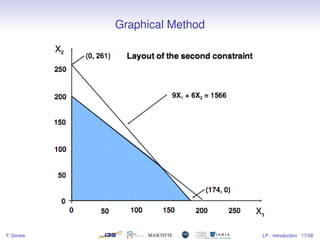
  • 18. Graphical Method Example: max 350x1 +300x2 subject to x1 +x2 ≤ 200 9x1 +6x2 ≤ 1566 12x1 +16x2 ≤ 2880 x1,x2 ≥ 0 F. Giroire LP - Introduction 15/28
  • 19. Graphical Method F. Giroire LP - Introduction 16/28
  • 20. Graphical Method F. Giroire LP - Introduction 17/28
  • 21. Graphical Method F. Giroire LP - Introduction 18/28
  • 22. Graphical Method F. Giroire LP - Introduction 19/28
  • 23. Graphical Method F. Giroire LP - Introduction 20/28
  • 24. Graphical Method F. Giroire LP - Introduction 21/28
  • 25. Computation of the optimal solution The optimal solution is at the intersection of the constraints: x1 +x2 = 200 (2) 9x1 +6x2 = 1566 (3) We get: x1 = 122 x2 = 78 Objective = 66100. F. Giroire LP - Introduction 22/28
  • 26. Optimal Solutions: Different Cases F. Giroire LP - Introduction 23/28
  • 27. Optimal Solutions: Different Cases Three different possible cases: • a single optimal solution, • an infinite number of optimal solutions, or • no optimal solutions. F. Giroire LP - Introduction 23/28
  • 28. Optimal Solutions: Different Cases Three different possible cases: • a single optimal solution, • an infinite number of optimal solutions, or • no optimal solutions. If an optimal solution exists, there is always a corner point optimal solution! F. Giroire LP - Introduction 23/28
  • 29. Solving Linear Programmes F. Giroire LP - Introduction 24/28
  • 30. Solving Linear Programmes • The constraints of an LP give rise to a geometrical shape: a polyhedron. • If we can determine all the corner points of the polyhedron, then we calculate the objective function at these points and take the best one as our optimal solution. • The Simplex Method intelligently moves from corner to corner until it can prove that it has found the optimal solution. F. Giroire LP - Introduction 25/28
  • 31. Solving Linear Programmes • Geometric method impossible in higher dimensions • Algebraical methods: • Simplex method (George B. Dantzig 1949): skim through the feasible solution polytope. Similar to a "Gaussian elimination". Very good in practice, but can take an exponential time. • Polynomial methods exist: • Leonid Khachiyan 1979: ellipsoid method. But more theoretical than practical. • Narendra Karmarkar 1984: a new interior method. Can be used in practice. F. Giroire LP - Introduction 26/28
  • 32. But Integer Programming (IP) is different! • Feasible region: a set of discrete points. • Corner point solution not assured. • No "efficient" way to solve an IP. • Solving it as an LP provides a relaxation and a bound on the solution. F. Giroire LP - Introduction 27/28
  • 33. Summary: To be remembered • What is a linear programme. • The graphical method of resolution. • Linear programs can be solved efficiently (polynomial). • Integer programs are a lot harder (in general no polynomial algorithms). In this case, we look for approximate solutions. F. Giroire LP - Introduction 28/28