


![Peano-Hilbert curve
The Peano-Hilbert curves were discovered by Peano and
Hilbert in 1890/1891
They convert against a function which maps the interval
[0,1] of the real numbers surjective on the area [0,1] x [0,1]
and is in the same time constant
That means through repeatedly execute the function rules
you will reach every point in a square
23/10/2018 Lecture 2 Algorithm Part 1 40](https://image.slidesharecdn.com/lecture2aalgorithm-181023121505/85/Lecture2a-algorithm-40-320.jpg)


Lecture2a algorithm
- 1. Lecture 2 Algorithm Part 1 23/10/2018 Lecture 2 Algorithm Part 1 1
- 2. Content Lecture 2 Part 1 Performance Introduction Recursive Examples Recursion vs. Iteration Primitive Recursion Function Peano-Hilbert Curve Turtle Graphics 23/10/2018 Lecture 2 Algorithm Part 1 2
- 3. Performance Performance in computer system plays a significant rule The performance is general presented in the O-Notation (invented 1894 by Paul Bachmann) called Big-O-Notation Big-O-Notation describes the limiting behavior of a function when the argument tends towards a particular value or infinity Big-O-Notation is nowadays mostly used to express the worst case or average case running time or memory usage of an algorithm in a way that is independent of computer architecture This helps to compare the general effectiveness of an algorithm 23/10/2018 Lecture 2 Algorithm Part 1 3
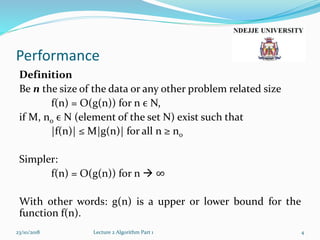
- 4. Performance Definition Be n the size of the data or any other problem related size f(n) = O(g(n)) for n ϵ N, if M, n0 ϵ N (element of the set N) exist such that |f(n)| ≤ M|g(n)| for all n ≥ n0 Simpler: f(n) = O(g(n)) for n ∞ With other words: g(n) is a upper or lower bound for the function f(n). 23/10/2018 Lecture 2 Algorithm Part 1 4
- 5. Performance The formal definition of Big-O-Notation is not used directly The Big-O-Notation for a function f(x) is derived by the following rules: If f(x) is a sum of several terms the one with the largest growth rate is kept and all others are ignored If f(x) is a product of several factors, any constants (independent of x) are ignored 23/10/2018 Lecture 2 Algorithm Part 1 5
- 6. Performance Example f(x) = 7x3 – 3x2 + 11 The function is the sum of three terms: 7x3, -3x2, 11 The one with the largest growth rate it the one with the largest exponent: 7x3 This term is a product of 7 and x3 Because the factor 7 doesn’t depend on x it can be ignored As a result you got: f(x) = O(g(x)) = O(x3) with g(x) = x3 23/10/2018 Lecture 2 Algorithm Part 1 6
- 7. Performance List of standard Big-O Notations for comparing algorithm: O(1) Constant effort, independent from n O(n) Linear effort 23/10/2018 Lecture 2 Algorithm Part 1 7
- 8. Performance O(n log(n)) Effort of good sort methods O(n2) Quadratic effort 23/10/2018 Lecture 2 Algorithm Part 1 8
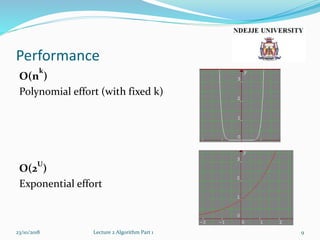
- 9. Performance O(n k ) Polynomial effort (with fixed k) O(2 U ) Exponential effort 23/10/2018 Lecture 2 Algorithm Part 1 9
- 10. Performance O(n!) All permutation of n elements Worst case! 23/10/2018 Lecture 2 Algorithm Part 1 10
- 11. Performance Other performance notations theta sigma small-o 23/10/2018 Lecture 2 Algorithm Part 1 11
- 12. Algorithm What is an algorithm? 23/10/2018 Lecture 2 Algorithm Part 1 12
- 13. Algorithm A set of instructions done sequentially A list of well-defined instructions to complete a given task To perform a specified task in a specific order It is an effective method to solve a problem expressed as a finite sequence of steps It is not limited to finite (nondeterministic algorithm) In computer systems an algorithm is defined as an instance of logic written in software in order to intend the computer machine to do something 23/10/2018 Lecture 2 Algorithm Part 1 13
- 14. Algorithm It is important to define the algorithm rigorously that means that all possible circumstances for the given task should be handled There is an initial state The introductions are done as a series of steps The criteria for each step must be clear and computable The order of the steps performed is always critical to the algorithm The flow of control is from the top to the bottom (top- down) that means from a start state to an end state Termination might be given to the algorithm but some algorithm could also run forever without termination 23/10/2018 Lecture 2 Algorithm Part 1 14
- 15. Algorithm All algorithms are classified in 6 classes: Recursion vs. Iteration Logical Serial(Sequential)/Parallel/Distributed Deterministic/Non-deterministic Exact/Approximate Quantum 23/10/2018 Lecture 2 Algorithm Part 1 15
- 16. Algorithm Recursion vs. Iteration Recursive algorithm makes references to itself repeatedly until a finale state is reached Iterative algorithms use repetitive constructs like loops and sometimes additional data structures More details later Logical Algorithm = logic + control The logic component defines the axioms that are used in the computation, the control components determines the way in which deduction is applied to the axioms Example The programming language Prolog 23/10/2018 Lecture 2 Algorithm Part 1 16
- 17. Algorithm Serial(Sequential)/Parallel/Distributed Serial Algorithm performing tasks serial that means one step by one step; Each step is a single operation Parallel Algorithm performing multiple operations in each step Distributed Algorithm performing tasks distributed Examples Serial: Calculating the sum of n numbers Parallel: Network Distributed: GUI, E-mail 23/10/2018 Lecture 2 Algorithm Part 1 17
- 18. Algorithm Deterministic/Non-deterministic Deterministic algorithm solve the problem with exact decision at every step Non-deterministic solve problem by guessing through the use of heuristics Example Shopping List Buy all items in any order nondeterministic algorithm Buy all items in a given order deterministic algorithm Exact/Approximate Exact algorithms reach an exact solution Approximation algorithms searching for an approximation close to the true solution 23/10/2018 Lecture 2 Algorithm Part 1 18
- 19. Algorithm Example: To find an approximate solutions to optimization problems like storehouses for shops Quantum Quantum algorithm running on a realistic model of quantum computation It is a step-by-step procedure, where each of the steps can be performed on a quantum computer It might be able to solve some problems faster than classical algorithms Example: Shor's algorithm for integer factorization 23/10/2018 Lecture 2 Algorithm Part 1 19
- 20. Recursion Many problems, models and phenomenon have a self-reflecting form in which the own structure is contained in different variants This can be a mathematical formula as well as a natural phenomenon If this structure is adopted in a mathematical definition, an algorithm or a data structure than this is called a recursion 23/10/2018 Lecture 2 Algorithm Part 1 20
- 21. Recursion Definition Recursion is the process of repeating items in a self-similar way. Recursion definitions are only reasonable if something is only defined by himself in a simpler form The limit will be a trivial case This case needs no recursion anymore A common joke is the following "definition" of recursion (Catb.org. Retrieved 2010-04-07.): Recursion See "Recursion" 23/10/2018 Lecture 2 Algorithm Part 1 21
- 22. Recursion Examples Language A child couldn't sleep, so her mother told a story about a little frog, who couldn't sleep, so the frog's mother told a story about a little bear, who couldn't sleep, so bear's mother told a story about a little weasel ...who fell asleep. ...and the little bear fell asleep; ...and the little frog fell asleep; ...and the child fell asleep. 23/10/2018 Lecture 2 Algorithm Part 1 22
- 23. Mathematical examples Factorial The Factorial of a number if defined as n! = n*(n-1)*(n-2)*…*1 Therefore: F(n) = n! for n > 0 is defined: F(1) = 1 F(n) = n * F(n-1) for n > 1 Program code in C/C++ int factorial(int number) { if (number <= 1) //trivial case return number; return number * (factorial(number - 1)); //recursive call } 23/10/2018 Lecture 2 Algorithm Part 1 23
- 24. Mathematical examples Calculate F(5) = 5! = 120 23/10/2018 Lecture 2 Algorithm Part 1 24
- 25. Recursion Because of recursion it is possible that more than one incarnation of the procedure exists at one time It is important that there is finiteness in the recursion (a trivial case) For example a query decided if there is another recursion call or not Otherwise you will have an endless recursive algorithm calling itself again and again In the example it was the case that number <= 1 23/10/2018 Lecture 2 Algorithm Part 1 25
- 26. Recursion Definition The depth of a recursion is the number of recursion calls. Example For factorial the depth of F(n) is n. depth(F(n)) = n Because in every step you call the recursion only one time. Therefore depth(F(5)) = 5 23/10/2018 Lecture 2 Algorithm Part 1 26
- 27. Recursion There are two ways to implement a recursion: Starting from an initial state and deriving new states which every use of the recursion rules Starting from a complex state and simplifying successive through using the recursion rules until a trivial state is reached which needs no use of recursion (see Faculty) How to build a recursion depends mainly on: How readable and understandable the alternative variants are Performance and memory issues 23/10/2018 Lecture 2 Algorithm Part 1 27
- 28. Mathematical examples Greatest Common Divisor The Greatest Common Divisor gcd(x,y) of the integer x and y s is the product of all common prime number factors of x and y To calculate the gcd you can use the following formula: gcd(x1, y1) = gcd(y1, x1 % y1) =gcd(x2, y2) = = gcd(y2, x2 % y2) = … = gcd(xk, 0) The final gcd(xk, 0) = xk is the Greatest common divisor 23/10/2018 Lecture 2 Algorithm Part 1 28
- 29. Mathematical examples Implementation in C int mygcd(int x, int y) { if (y == 0) //trivial case return x; else return mygcd(y, x % y); //recursive call } gcd(34, 16) = gcd(16, 2) = gcd(2, 0) = 2 gcd(127, 36)=gcd(36, 19)=gcd(19, 17)=gcd(17, 2)=gcd(2, 1)=gcd(1, 0)=1 23/10/2018 Lecture 2 Algorithm Part 1 29
- 30. Mathematical examples Fibonacci sequence Fibonacci sequence is one of the classical example of recursion Leonardo Fibonacci was an Italian mathematician (around 1180 – 1240) The Fibonacci sequence can be found also in nature (plants) The sequence is defined as: F(0) = 0 (base case) F(1) = 1 (base case) F(n) = F(n-1) + F(n-2) (recursion) for all n > 1 with n ϵ N 23/10/2018 Lecture 2 Algorithm Part 1 30
- 31. Mathematical examples Calculate F(4) = 3 23/10/2018 Lecture 2 Algorithm Part 1 31
- 32. Mathematical examples Ackermann function Wilhelm Ackermann was a German mathematician (1896 – 1962) The Ackermann function is used as a benchmark of the ability of a compiler to optimize recursion The function is defined as: 𝐴 𝑚, 𝑛 = 𝑛 + 1 𝑖𝑓 𝑚 = 0 𝐴 𝑚 − 1, 1 𝑖𝑓 𝑚 > 0 𝑎𝑛𝑑 𝑛 = 0 𝐴 𝑚 − 1, 𝐴 𝑚, 𝑛 − 1 𝑖𝑓 𝑚 > 0 𝑎𝑛𝑑 𝑛 > 0 23/10/2018 Lecture 2 Algorithm Part 1 32
- 33. Mathematical examples Implementation in C int ackermann(int m, int n) { if (m == 0) //trivial case return n + 1; else if (n == 0) //recursive call return ackermann(m – 1, 1); else //recursive call return ackermann(m – 1, ackermann(m, n – 1)); } 23/10/2018 Lecture 2 Algorithm Part 1 33
- 34. Recursion vs. Iteration Use of recursion in an algorithm has both advantages and disadvantages The main advantage is usually simplicity The main disadvantage is often that the algorithm may require large amounts of memory if the depth of the recursion is very high Many problems are solved more elegant and efficient if they are implemented by using iteration This is especially the case for tail recursions which can be replaced immediately by a loop, because no nested case exists which has to be represented by a recursion The recursive call happens only at the end of the algorithm Recursion and iteration are not really contrasts because every recursion can also be implemented as iteration 23/10/2018 Lecture 2 Algorithm Part 1 34
- 35. Recursion vs. Iteration Tail recursion int tail_recursion(…) { if (simple_case) //trivial case /*do something */; else /*do something */; tail_recursion(…); // only recursive call } 23/10/2018 Lecture 2 Algorithm Part 1 35
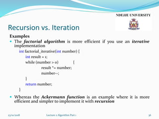
- 36. Recursion vs. Iteration Examples The factorial algorithm is more efficient if you use an iterative implementation int factorial_iterative(int number) { int result = 1; while (number > 0) { result *= number; number--; } return number; } Whereas the Ackermann function is an example where it is more efficient and simpler to implement it with recursion 23/10/2018 Lecture 2 Algorithm Part 1 36
- 37. Primitive Recursion Function Definition The primitive recursive functions are among the number- theoretic functions, which are functions from the natural numbers (non negative integers) {0, 1, 2 , ...} to the natural numbers These functions take n arguments for some natural number n and are called n-ary Functions in number theory are primitive recursive Important also in proof theory (proof by induction) 23/10/2018 Lecture 2 Algorithm Part 1 37
- 38. Primitive Recursion Function The basic primitive recursive functions are given by these axioms: Constant function: The 0-ary constant function 0 is primitive recursive Successor function: The 1-ary successor function S, which returns the successor of its argument, is primitive recursive. That is, S(k) = k + 1 Projection function: For every n ≥ 1 and each i with 1 ≤ i ≤ n, the n-ary projection function Pi n, which returns its ith argument, is primitive recursive 23/10/2018 Lecture 2 Algorithm Part 1 38
- 39. Primitive Recursion Function Examples Addition: x + y Add(0, x) = x Add(y + 1, x) = Add(y, x) + 1 Multiplication: x*y Exponentiation: xy, Factorial: n! Minimum: (n1, ... nn) Maximum: (n1, ... nn) 23/10/2018 Lecture 2 Algorithm Part 1 39
- 40. Peano-Hilbert curve The Peano-Hilbert curves were discovered by Peano and Hilbert in 1890/1891 They convert against a function which maps the interval [0,1] of the real numbers surjective on the area [0,1] x [0,1] and is in the same time constant That means through repeatedly execute the function rules you will reach every point in a square 23/10/2018 Lecture 2 Algorithm Part 1 40
- 41. Peano-Hilbert curve The Peano-Hilbert Curve can be expressed by a rewrite system (L- system): Alphabet: L, R Constants: F, +, − Axiom: L Production rules: L → +RF−LFL−FR+ R → −LF+RFR+FL− F: draw forward +: turn left 90° -: turn right 90° 23/10/2018 Lecture 2 Algorithm Part 1 41
- 42. Peano-Hilbert curve First order: L +F-F-F+ R -F+F+F- Second order: +RF-LFL-FR+ +-F+F+F-F-+F-F-F+F+F-F-F+-F-F+F+F-+ Used in computer science For example to map the range of IP addresses used by computers into a picture 23/10/2018 Lecture 2 Algorithm Part 1 42
- 43. Turtle Graphics Turtle Graphics are connected to the program language Logo (1967) There is no absolute position in a coordination system All introductions are relative to the actual position A simple form would be: Alphabet: X, Y Constants: F, +, − Production rules: Initial Value: FX X → X+YF+ Y → -FX-Y 23/10/2018 Lecture 2 Algorithm Part 1 43 F: draw forward +: turn left 90° -: turn right 90°
- 44. Turtle Graphics Level 1: FX = F+F+ Level 2: FX = FX+YF+ = F+F++-F-F+ 23/10/2018 Lecture 2 Algorithm Part 1 44
- 45. Turtle Graphics Other turtle graphic 23/10/2018 Lecture 2 Algorithm Part 1 45
- 46. Any questions? 23/10/2018 Lecture 2 Algorithm Part 1 46